Orbital decay in M82 X-2

Abstract

M82 X-2 is the first pulsating ultraluminous X-ray source (PULX) discovered. The luminosity of these extreme pulsars, if isotropic, implies an extreme mass transfer rate. An alternative is to assume a much lower mass transfer rate, but with an apparent luminosity boosted by geometrical beaming. Only an independent measurement of the mass transfer rate can help discriminate between these two scenarios. In this Paper, we follow the orbit of the neutron star for seven years, measure the decay of the orbit ($\dot{P}_{\rm orb}/P_{\rm orb}\approx-8\cdot 10^{-6}\,\mathrm{yr^{-1}}$), and argue that this orbital decay is driven by extreme mass transfer of more than 150 times the mass transfer limit set by the Eddington luminosity. If this is true, the mass available to the accretor is more than enough to justify its luminosity, with no need for beaming. This also strongly favors models where the accretor is a highly-magnetized neutron star.

1 Introduction

The luminosity of accreting sources is largely driven by the amount of matter that is transferred onto the accreting object, whether it be from a donor star for typical neutron stars and stellar mass black holes, or an accretion disk for supermassive black holes at the centers of galaxies (Frank et al., 2002). There is a classical limit to the mass transfer, which corresponds to the mass accretion rate that leads to a balance between the force of radiation pressure pushing outward and the gravitational force acting inward on an accreting object of mass $M$. For spherical hydrogen accretion, this corresponds to the Eddington luminosity:

$$L_{\rm Edd}\approx 1.3\cdot 10^{38}\frac{M}{M_{\odot}}\,\mathrm{erg\,s^{-1}}$$ (1)

Therefore, the extreme luminosity of ultraluminous X-ray sources (ULXs; Kaaret et al. 2017; Fabrika et al. 2021) led many to think that these sources were powered by intermediate-mass black holes. Over the years, multiple pieces of evidence cast doubt on the applicability of this classical limit on ULXs (Poutanen et al., 2007; Gladstone et al., 2009; Bachetti et al., 2013). Eventually, the discovery of pulsating ultraluminous X-ray sources (PULXs; Bachetti et al. 2014, hereafter B14), accreting neutron stars radiating hundreds of times above their Eddington limits, demonstrated that super-Eddington accretion was a viable explanation for the majority of ULXs. It is still unclear how these pulsars (pulsating neutron stars) emit this extreme luminosity. Some argue that the isotropic luminosity is much lower, and the observed luminosity is boosted by geometrical beaming, driven by the collimation of a (less extreme) super-Eddington disk (King et al., 2017). This interpretation has found some support in global MHD simulations of accreting black holes and neutron stars, where mild to extreme geometrical beaming is observed (e.g. Jiang et al. 2014; Abarca et al. 2021). However, these simulations assume a low magnetic field of the neutron star ($\lesssim 10^{10}$ G), if any, and this collimation effect is likely to be lessened when the magnetic field of the pulsar is stronger. In fact, other models explain the luminosity with arguments centered on a high magnetic field of the pulsar ($>10^{13}$ G), like the reduction of the Thomson scattering cross section in high magnetic fields, either in their dipolar (Mushtukov et al., 2015, 2017) or their multipolar components (Brice et al., 2021). This reduction of the cross section allows to hit the local Eddington limit at much higher mass accretion rates, increasing the maximum luminosity. It is also possible that the solution is a mixture of genuine super-Eddington accretion and a small amount of beaming (Israel et al., 2017).

A key difference between these models is the relation that they assume between the mass accretion rate $\dot{m}=\dot{M}/\dot{M}_{\rm Edd}$ and the luminosity, linear in the low-beaming scenario, almost quadratic ($L\propto(1+\log\dot{m})\dot{m}^{2}$) in the other, due to the assumed quadratic dependence of beaming on the mass accretion rate (King, 2008). In other words, beaming models infer a much lower mass transfer rate between the donor star and the neutron star for a given luminosity.

An independent measurement of the mass transfer is key for disentangling these two scenarios. In principle, one way to measure this transfer of matter between two orbiting objects is through the observation of a decay of the orbital period (Tauris & van den Heuvel, 2006).

One of the best systems where this can be tested is M82 X-2, the first pulsating ultraluminous X-ray source ever discovered. B14 and Bachetti et al. (2020) (hereafter B20) measured the orbit of this PULX very precisely, determining an orbital period of $2.532948(4)$ d, a semi-major axis of $22.215(5)$ light-sec, and no detectable eccentricity ($<$0.003). What makes this system particularly interesting from the point of view of orbital decay measurements is that its revolution period is short enough, and the ephemeris known so precisely, that the epoch of passage through the ascending node can be constrained to $\sim 100$ s with a single, reasonably long, X-ray observation.

In this Paper, by tracking the ascending node passages over 8 years of NuSTAR observations, we present the precise measurement of orbital decay in M82 X-2, leading to an estimate of mass transfer whose value agrees to within a factor 2 to the one inferred from the luminosity of the pulsar.

In Section 2 we describe the data reduction and in Section 3 we detail the temporal analysis that led to the orbital decay measurement, while we devote the last sections to the interpretation of this orbital decay.

2 Data reduction

2.1 NuSTAR

We downloaded all the NuSTAR data of M82 from the High Energy Astrophysics Science Archive Research Center (HEASARC). We ran nupipeline with standard options to produce cleaned event files. This tool produces different event files corresponding to different observing modes: SCIENCE (01), OCCULTATION (02), SLEW (03), SAA (04), CALIBRATION (05), and SCIENCE_SC (06). The modes usable for science are 01 and 06. Note, however, that only mode-01 data are recorded in normal instrumental conditions. Mode-06 data correspond to time intervals where only a subset of the camera head units (CHUs) are available, and the astrometry can be off by 1–2^′ (See Walton et al. 2016 for an example of the astrometry issues in this observing mode). For mode-01 data, we used a region of 70^′′ around the centroid of the X-ray source corresponding to the position of M82 X-1 and M82 X-2, which is spatially unresolved in NuSTAR. The centroid was calculated independently for each observation and for each of the two focal plane modules, as a mismatch of $\sim 10^{\prime\prime}$ can be expected.

We processed mode-06 data with the nusplitsc tool, which separates events corresponding to different CHU combinations. For each of these event files, we adjusted the centroid of the source and repeated the selection done for mode-01 data. Finally, we merged the source-selected event lists from mode-01 and mode-06 data. In only a few cases, due to the source falling on a chip gap, we saw that the light curve showed visible “steps” between intervals corresponding to different CHU combinations. We verified that the addition or elimination of the problematic intervals did not alter significantly the power around the pulsation frequency $\sim$0.7 Hz.

Finally, we ran barycorr to refer the photon arrival times to the solar system barycenter. We selected the ICRS reference frame, the DE421 JPL ephemeris, and the position of M82 X-2 determined by Chandra. For all observations, we used the latest clock correction file available, that provides an absolute time precision of $\sim 60\,\mu$s.

3 Timing analysis

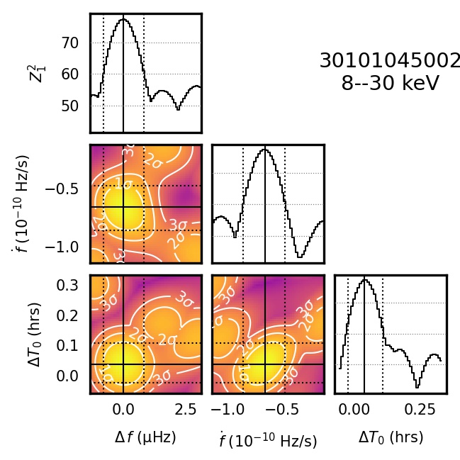
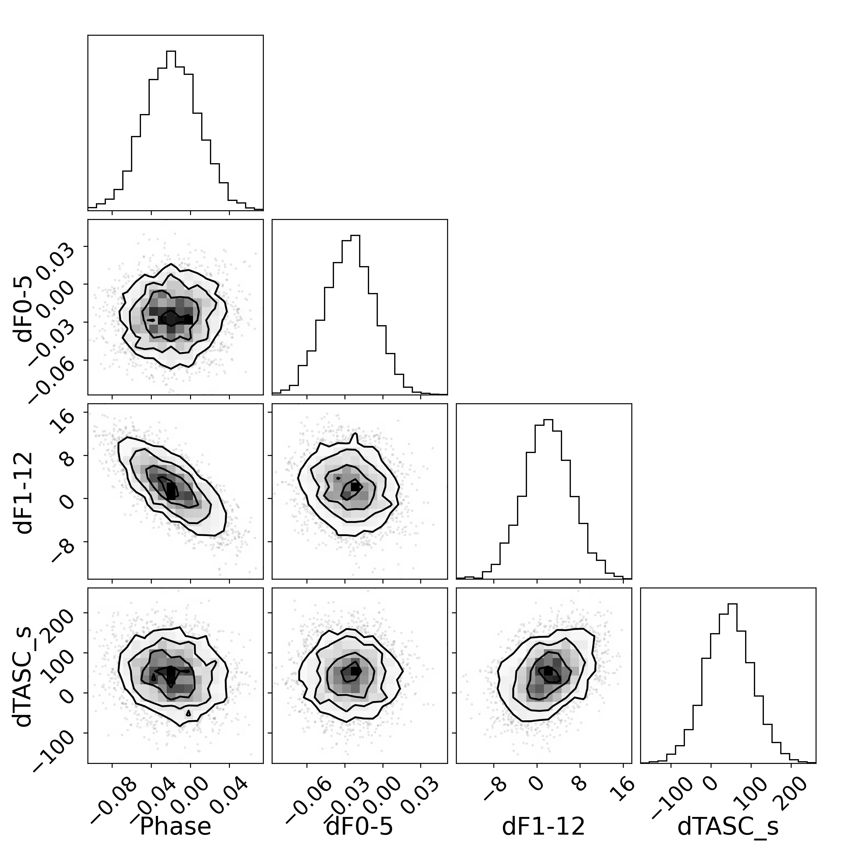
Figure 1: Example detection of pulsations, and orbital/spin parameter refinement, from ObsID 30101045002. The color map shows the Rayleigh search in a three-parameter grid, using spin-frequency, spin first derivative, and the drift of the periastron passage $T_{\rm asc}{}$. The corner plot on the right, instead, shows the refinement of the results of the Rayleigh search, with the addition of pulse phase, fitted using the Bayesian method by Pletsch & Clark (2015). E.g.: if dF0-5 is -0.03 and the initial F0 was 0.725, this means that the best-fit frequency is $0.725-0.03\cdot 10^{-5}$ Hz

Obs. ID	Epoch	Energy	$T_{\rm asc}$	$f_{\rm spin}$	$\dot{f}_{\rm spin}$	$\ddot{f}_{\rm spin}$	$\Delta\,T_{\rm asc}$ (s)
	MJD	keV	MJD	Hz	$10^{-12}$ Hz s-1	$10^{-16}$ Hz s-2	s
80002092002∗	56681.24441	8–30	56682.073(5)	0.728509(4)	-90(70)		600(500)
80002092004	56683.81009	8–30	56684.6004(28)	0.7285316(16)	50(35)		110(240)
80002092006	56688.80899	8–30	56689.6656(5)	0.72854791(22)	15.3(12)	1.20(27)	50(40)
80002092007	56694.12259	3–30	56694.73184(19)	0.72856174(6)	34.6(14)		86(17)
80002092007	56697.38070	3–30	56697.2648(4)	0.72857943(8)	92(6)		90(40)
80002092008	56700.75316	3–30	56699.798(5)	0.728609(5)	90(60)		100(400)
80002092009	56700.75316	3–30	56699.7978(4)	0.72860925(13)	106(5)		90(32)
80002092011	56720.87754	8–30	56720.0612(12)	0.7287596(6)	113(13)		80(100)
30101045002∗	57495.31178	8–30	57495.1440(7)	0.72519103(20)	-65(5)		140(60)
90201037002	57641.99852	8–30	57642.049(8)	0.7239040(12)	-320(230)		-400(700)
30502021002∗	58919.09530	3–30	58918.6261(12)	0.7219294(7)	36(15)		-2860(100)
30602027002∗	59312.65089	3–30	59313.750(6)	0.7222096(21)	120(150)		-4300(500)
30602027004∗	59326.05680	8–30	59326.409(4)	0.7222978(25)	50(70)		-4700(400)
30702012002∗	59505.27806	3–30	59506.2428(11)	0.72086594(33)	-45(14)		-5210(90)

Table 1: Spin and orbital parameters from the multidimensional timing procedure in Section 3. Starred ObsIDs are those corresponding to new detections from this paper. We also highlight in bold observations with significant ($>3\sigma$) evidence of spin down. The energy range is the one where the pulsations are detected with the highest significance. Data from ObsID 80002092006 start after the glitch reported by B20 at MJD 56685.7 ObsID 80002092007 has a sudden change of frequency, probably another glitch, around MJD 56696, therefore we split the observation in two parts around that epoch. $\Delta\,T_{\rm asc}$ was calculated with respect to the orbital ephemeris from B20

Due to the very low pulsed fraction in the XMM-Newton band, demonstrated in Appendix F, we only used NuSTAR data for Timing analysis.

Initially, we largely followed the search strategies used in B20, running $Z^{2}_{1}$ searches (Buccheri et al., 1983), also known as the Rayleigh test, on the event arrival times corrected for orbital motion, varying the ascending node passage epoch $T_{\rm asc}{}$ on a fine grid between $-P_{\rm orb}/5$ and $P_{\rm orb}/5$. This time, the search allowed a range of spin derivatives for each trial ascending node passage value. The spin parameters vary so rapidly that they are only loosely constrained when observations are just a $\sim$week apart. There is no way to reliably phase connect separate observations. Therefore, even observations done $\sim 2$ weeks apart were analyzed singularly. For the search in the $f-\dot{f}$ plane, we used the “quasi-fast folding algorithm” (B20), that calculates the $Z^{2}_{1}$ on pre-binned profiles (Bachetti et al., 2021), using at least 16 bins for the folded profiles. Moreover, we ran the search both in the full energy band and between 8 and 30 keV. This allowed four detections in the new observations. We also re-ran a pulsation search using all available observations, and we found highly significant ($\geq 5\sigma$) pulsations in two archival datasets, corresponding to ObsIDs 30101045002 and 80002092002. In both observations, pulsations are more strongly detected in the 8–30 keV energy band. Moreover, surprisingly, we find that during 30101045002 the pulsar was instantaneously spinning down. This is the first time that M82 X-2 is found spinning down while accreting and pulsating, and provides clear evidence that a significant part of the torque from the disk is happening outside the corotation radius (see Appendix C for more details). This is probably why B20 only obtained marginal evidence for pulsations in this ObsID. This new detection is important because pulsations are detected over a $\sim 4$-day interval, which is long enough to provide an excellent constraint on $T_{\rm asc}{}$. For each detection, we then ran the search again around the best solution, oversampling by a large factor to find the best estimate of the mean of each parameter.

We proceeded to create local timing solutions for each observation, leaving the orbital parameters from B20 unchanged with the exception of the ascending node, and setting the current spin frequency and frequency derivative. These local solutions differed only for the parameters F0 (spin frequency in Hz), F1 (spin derivative in Hz/s), and TASC (ascending node passage in MJD). Then, we used the method by Pletsch & Clark (2015) to make a Bayesian fit of the local timing solution, using a sinusoidal pulse template normalized to the same pulsed fraction of the pulsar in each given observation. Working in phase space instead of frequency, this method is far more sensitive to small changes of parameters, and yields very precise estimates on them. The exact parameters we fitted were the difference from F0 in units of $10^{-X}$ s, depending on the observation length, the difference from F1 in units of $10^{-Y}$ Hz/s (where $X,Y$ were chosen as values close to the order of magnitude of the known errors on the parameters), and the difference from TASC in seconds. This was done to avoid incurring in numerical errors due to the small steps involved in some parameters. We set flat priors for all parameters: $0.5<f<1$ Hz, $|\dot{f}|<10^{-7}$ and $\Delta T_{\rm asc}{}<P_{\rm orb}$. We first used the scipy.optimize.minimize function to minimize the negative log-likelihood and determine an approximate starting solution. Then, values around this solution was used to initialize a Markov Chain Monte Carlo (MCMC) sampler as implemented in the emcee (Foreman-Mackey et al., 2013) library. Since the analysis took a significant time (up to 2 s per iteration in the larger datasets), we followed the instructions in the emcee documentation to interrupt the sampling once the iterations had reached 200 times the the “autocorrelation time” $\tau$, more than the recommended 50 for additional robustness. $\tau$ itself was calculated every 100 steps of the chain. The number of steps used in the chains varied between 3,000 and 100,000 depending mostly on the length of the observation and the number of photons, with longer observations requiring fewer steps (because of the reduced correlations between parameters). We used the 3-30 keV or 8-30 keV energy range depending on which range yielded the highest power in the Rayleigh search. This allowed to estimate the posterior distribution on the parameters, and their uncertainties. The posterior distributions are generally well-behaved, with reasonably (sometimes slightly skewed due to the correlation between the parameters) bell-shaped distributions. We determined 1-$\sigma$ error bars on the parameters by looking at the 16% and 84% percentiles. The results are summarized in Table 1, and the detection in ObsID 30101045002 is shown in Figure 1 as an example.

3.1 Orbital decay

To describe a change of the orbital period over time, it is customary to measure the time that a star reaches a particular phase of the orbit, and compare it with the expected time given the previous orbital solution. For circular orbits with no eclipses, it is common to use one of the two intersections between the orbit and the plane perpendicular to the line of sight passing through the center of mass of the binary system. These points of the orbit are called nodes; the ascending node is the node that the pulsar crosses when moving away from the observer. The expected time of passage at the ascending node after $n$ orbits $T_{\rm asc,n}$ (for simplicity, we drop the asc when $n$ or other indices are present), in the presence of an orbital derivative, can be expressed as (cfr. Kelley et al. 1980; Falanga et al. 2015):

$$T_{n}=T_{0}+n\,P_{\rm orb}+\frac{1}{2}\,n^{2}\,P_{\rm orb}\,\dot{P}_{\rm orb}+\,\frac{1}{6}\,n^{3}P_{\rm orb}^{2}\,\ddot{P}_{\rm orb}+\dots$$ (2)

By using a previously determined ephemeris as a baseline, we can measure the delay of the measured $T_{\rm asc}{}$ from the expected one. When plotting this delay, offsets indicate a shift in $T_{\rm asc}{}$, linear trends an uncertainty of $P_{\rm orb}$, and parabolic trends an orbital period derivative:

$$\delta T_{n}(t)=\delta T_{\rm asc}{}+\frac{t-T_{\rm asc}{}}{P_{\rm orb}}\delta{P_{\rm orb}}+\frac{1}{2}\frac{\dot{P}_{\rm orb}}{P_{\rm orb}}\left(t-T_{\rm asc}{}\right)^{2},$$ (3)

where we substituted $n=(t-T_{\rm asc}{})/P_{\rm orb}$.

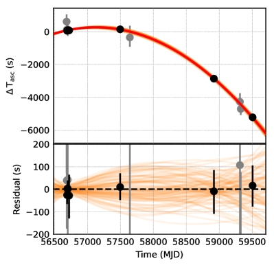
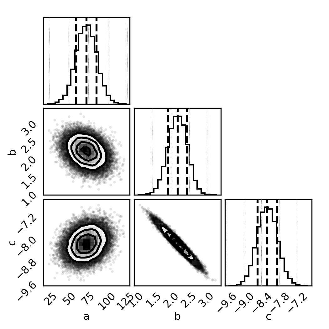
Figure 2: (Left) Orbital decay in M82 X-2, measured through the delay of the $T_{\rm asc}{}$ parameter (time of passage through the ascending node) from Equation 3. Semi-transparent orange lines indicate possible $\sim$1000 quadratic solutions, coming from MCMC sampling (described in Section 3.1). Grey points are lower-quality measurements (uncertainty in $T_{\rm asc}{}$larger than 200 s due to high orbital-spin parameter correlation). (Right) Corner plot of the posterior distribution of the parameters of the orbital decay with Equation 4, sampled with MCMC. Vertical dashed lines show the 16%, 50%, and 84% percentiles.

Using the new $T_{\rm asc}$ values, we infer the orbital decay of M82 X-2 using a Bayesian model.

The following equation serves as the orbital evolution model:

$$\Delta T_{\rm asc}{}=a+\frac{b}{P_{\rm orb}}(t-T_{\rm asc}{})+0.5\cdot 10^{-6}\,c\,\frac{86400}{365.25}(t-T_{\rm asc}{})^{2}$$ (4)

where $t$, $T_{\rm asc}{}$ and $P_{\rm orb}$ are expressed in days, $\Delta T_{\rm asc}{}$ is the delay of $T_{\rm asc}{}$ in seconds, $a$ is a correction to $T_{\rm asc}{}$ in seconds, $b$ is a correction to $P_{\rm orb}$ in seconds and $c$ is the new value of $\dot{P}_{\rm orb}/P_{\rm orb}$ in units of $10^{-6}\,\mathrm{yr^{-1}}$. The baseline solution from B20 was $T_{\rm asc}{}_{,\rm B20}=\mathrm{MJD}\,56682.0661$, $P_{\rm orb,B20}=2.532948$ d, and $\dot{P}_{\rm orb}=0$ s s^-1. Priors for $a$, $b$ and $c$ were uniform between $\pm 10^{6}$; in checks, we found that the width of the prior has no significant effect on our posterior inference.

Parameter	Unit	Value (uncert)
$P_{\rm orb}$	d	2.5329733(30)
$\dot{P}_{\rm orb}$	s s-1	$-5.69(24)\cdot 10^{-8}$
$\dot{P}_{\rm orb}/P_{\rm orb}$	yr-1	$-8.20(34)\cdot 10^{-6}$
$a\sin i$	l-sec	22.218(5)
$T_{\rm asc}{}$	MJD	56682.06694(15)
$e$		$<0.0015$ (3-$\sigma$ u.l.)

Table 2: Updated orbital parameters for M82 X-2, as determined in this work.

We first performed a Maximum-A-Posteriori fit with a standard Gaussian likelihood, allowing for asymmetric error bars. The solution served as an initialization of a Markov Chain Monte Carlo (MCMC) sampler using emcee as before. Using 32 walkers, we ran the chains for 20000 steps. We calculated the autocorrelation “time”, which was at most 46 steps. We thinned the chain by a factor 23 (half the autocorrelation length) and discarded 920 steps (20 times the autocorrelation length) as burn-in. The resulting marginal posterior probability distributions are plotted using the corner library (Foreman-Mackey, 2016) in Figure  2.

We find posterior means and credible intervals of $a=72(13)$, $b=2.18(26)$, and $c=-8.20(34)$. Using these values, we corrected the orbital parameters as $T_{\rm asc}{}=T_{0,\rm B20}+a\,\mathrm{sec}$, $P_{\rm orb}=P_{\rm orb,B20}+b\,\mathrm{sec}$, $\dot{P}_{\rm orb}/P_{\rm orb}=c\cdot 10^{-6}{\rm yr}^{-1}$ to obtain the values in Table 2.

Finally, we fixed the orbital parameters and we re-ran a final accelerated search for pulsations in all ObsIDs using the Rayleigh test, yielding the results in Table 1.

4 Discussion

Over the years, many models have been proposed to describe the interaction between the plasma in the disk and the magnetic field lines of an accreting pulsar (Ghosh & Lamb, 1978; Wang, 1996; Chashkina et al., 2017). Despite large differences in the treatment of the details of this interaction, these models make estimates for the magnetic field within $\sim$one order of magnitude when the inner radius and the mass accretion rate are fixed (Xu & Li, 2017; Chen et al., 2021; Erkut et al., 2020), if one can assume spin equilibrium: a regime where the outward pressure from the rotating magnetic field balances almost exactly the ram pressure from the infalling matter.

Until now, different groups have used the observed luminosity as a proxy for the mass accretion rate, and this produced very different estimates depending on the assumption of the beaming fraction. In addition, different works used different assumptions on the position of the inner radius, with the high-magnetic field models assuming spin equilibrium (Ekşi et al., 2015; Tsygankov et al., 2016; Dall’Osso et al., 2015) and the beaming models being incompatible with it (King et al., 2017).

In this work, we produce robust evidence in favor of spin equilibrium, and we measure an orbital decay that might provide an independent estimate of mass transfer, as we are going to discuss below.

4.1 Spin equilibrium

Thanks to the new detections listed above, we found that for at least part of the time between 2016 and 2020 the pulsar continued to spin down (slow down its rotation) as reported by B20, because the frequency ($\sim 0.721$ Hz) observed in 2020 was lower than observed in 2016 ($\sim 0.723$ Hz). However, since then, the neutron star appears to be alternating phases of spin up and spin down around $\sim 0.721$ Hz. In at least one observation in 2016 and probably in another in 2021, the pulsar was spinning down while accreting (see Table 1). In summary, the spin evolution of M82 X-2 strongly points to a situation of spin equilibrium. In this condition, spin up and spin down can be produced with small changes of accretion rate (D’Angelo & Spruit, 2012), and it is possible to confidently estimate the magnetic field of the neutron star, by equating the analytical formulas for the inner radius $R_{\rm in}$ to the corotation radius $R_{\rm co}$, at which the angular velocity of the matter in the disk equals the one of the star (see Section C).

Being close to spin equilibrium also implies that a relatively small drop of mass accretion rate could trigger the so-called “propeller” regime (Illarionov & Sunyaev, 1975), where the rotating, highly-magnetized pulsar is able to swipe away the infalling matter. During the transition to this regime, it is possible to still have accretion, albeit discontinuous (Romanova et al., 2004), up to a point where accretion is stopped altogether leaving only the disk and the ejected matter as sources of X-ray flux. Based on a possible bimodal distribution of the fluxes of M82 X-2, Tsygankov et al. (2016) claimed that the observed low states in M82 X-2 were evidence of this transition. It is not clear, at the moment, if this is compatible with the observed $\sim 60$-day periodicity of the low states (Brightman et al., 2019), which would imply a periodic decrease of mass transfer, difficult to reconcile with the very low eccentricity of the system.

4.2 Is it mass transfer?

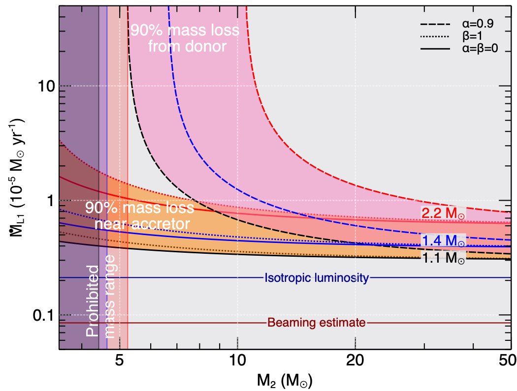
Figure 3: Mass transfer rate towards the accretor (through L1), versus donor mass, given the measured orbital period decay. We estimate the mass transfer rate for different mechanisms of mass loss and different accretor masses. Solid lines indicate conservative mass transfer, dashed lines indicate 90% isotropic mass loss from the donor, and dotted lines indicate 100% mass loss from the proximity of the accretor. The latter is only a small correction to the conservative case, while mass loss from the donor implies a much larger mass transfer rate in order to produce the observed orbital decay. Vertical bands on the left show the limit donor masses given the absence of eclipses, for different accretor masses (same color coding).

The observed orbital decay is compatible with the mass transfer from a more massive donor star to a neutron star (Tauris & van den Heuvel 2006, see Section B). Assuming a pulsar mass $M_{p}=1.4M_{\odot}$ and a donor mass $M_{d}=8M_{\odot}$ (which corresponds to the mean of the probability distributions of masses, see Section D), it is straightforward to estimate the mass transfer rate from the observed orbital decay, assuming conservative mass transfer, as $\dot{M}_{d}\approx-4.7\cdot 10^{-6}M_{\odot}\,\mathrm{yr^{-1}}$. This corresponds to $\sim 200$ times the Eddington limit, assuming an Eddington mass accretion rate corresponding to $\dot{M}_{\rm Edd}\approx 1.5\cdot 10^{18}\,{\rm g~{}s^{-1}}\approx 2.4\cdot 10^{-8}\,{M_{\odot}\rm yr^{-1}}$. This is the mass that the donor transfers into the Roche lobe of the neutron star. This mass exchange exceeds both that inferred from the apparent bolometric luminosity of the source (which is at most $\sim 100$ times the Eddington limit, see B14), or the one inferred from beaming scenarios (36 times Eddington, King et al. 2017). See Figure 3 for details. It is possible that part of this matter leaves the system through fast winds launched from the super-Eddington disk (Pinto et al., 2016; Kosec et al., 2018). This mass loss happens from the vicinity of the accretor, and its specific angular momentum is such that the effect on the orbit is similar to the conservative case (see Appendix B). On the other hand, it decreases the amount of matter that accretes onto the neutron star, which is a viable explanation for the slightly lower luminosity observed. Isotropic mass loss from the donor, instead, as one would expect from stellar winds, would have the opposite effect, expanding the orbit. Additional mass loss from the outer disk in the form of slow winds (e.g. Middleton et al., 2022) would represent an intermediate case, carrying away specific angular momentum somewhere between that at the position of the neutron star and that at L1. Therefore, the estimate above is a lower limit to the mass transfer rate. Another possibility, involving mass loss from L2 forming a circumbinary disk, is discussed below.

If the observed orbital decay really is due to mass transfer, we can fix these two important variables, leading to an interpretation of M82 X-2 being a highly magnetized neutron star ($B>10^{13}$ G) with any of these models (see also Appendix E), and exclude beaming as a primary amplifier of ULX emission (also see Vasilopoulos et al. 2021 for further evidence in this sense).

4.3 Alternative models

4.3.1 Synchronization and circularization

The value of orbital derivative found in this work is larger, albeit only by a few times, than those observed in much less luminous X-ray pulsars such as SMC X-1, LMC X-4, and Cen X-3 ($-3.5$, $-1.0$, and $-1.8\cdot 10^{-6}\,\mathrm{yr^{-1}}$ respectively, see Falanga et al. 2015). The slight mismatch that we find in M82 X-2 between the mass transfer inferred from the orbit and that inferred from the luminosity becomes a factor $\sim$20 for SMC X-1. This has led Falanga and many other authors (Levine et al., 2000, 1993; Chernov, 2020, e.g.) to disregard mass transfer as the primary engine for orbital decay in these systems. At this point, we cannot exclude that whatever process believed to be in place in those systems (like viscous processes producing the circularization of an elliptical orbit or the synchronization of the star’s rotation with the orbit, e.g. Falanga et al. 2015 and references therein; Chernov 2020) is at work in M82 X-2. However, we do stress that these HMXBs are likely accreting in very different regimes, possibly from focused winds and not from a Roche-Lobe overflow, as would instead be expected from a super-Eddington source.

4.3.2 Circumbinary disk

The observed orbital decay is, in principle, compatible with an equatorial circumbinary disk launched by the second Lagrangian point L2 (Tauris & van den Heuvel 2006, see also Appendix B. However, this only happens in situations where the donor star inflates well beyond its Roche Lobe, or via a fast and stable wind, and its onset quickly leads to unstable orbital decay and common envelope (Misra et al., 2020). Lu et al. (2022) study in detail the conditions for this phenomenon, finding that it should be important above $\dot{m}\sim 10^{-4}M_{\odot}\,\mathrm{yr^{-1}}$. SS433, a possible ULX analog in our Galaxy (Fabrika et al., 2006; Middleton et al., 2021), might be undergoing such a process. However, in that case, the accretor is believed to be a stellar-mass black hole (Blundell et al., 2008) and the mass ratio is $\sim 1$, and this process leads to the expansion of the orbit (Cherepashchuk et al., 2021), stabilizing the mass transfer.

5 Conclusion

The detection of orbital decay in M82 X-2 is a key milestone to understand the evolution of this system and, possibly, of all low-orbital period PULXs like NGC 5907 ULX1 (Israel et al., 2017) and M51 ULX-7 (Rodríguez Castillo et al., 2020).

We argue that the decay is driven by mass transfer: the implied mass transfer is only a factor $\sim 2$ above the one inferred from the luminosity, and this can easily be explained by a slightly lower efficiency or a massive outflow such as those observed in other ULXs (but undetectable in M82 X-2 due to source confusion in the M82 field). Currently, we cannot exclude that phenomena such as the synchronization of the donor rotation with the orbit and/or the circularization of the orbit are contributing to the observed decay, which is only a few times higher than that of the eclipsing HMXBs from Falanga et al. (2015). Note however that this source has a quite tight upper limit on the eccentricity (see Appendix A) and the accretion is very likely through Roche Lobe overflow, at a much higher rate than the sample from Falanga et al. (2015), making the timescale for synchronization faster. If these phenomena are in place, it is likely that we are witnessing a very short-lived phase of the evolution of this binary system.

Regardless of the exact driver of the observed orbital decay, our measurement informs the theoretical study of ULX progenitors. At the moment, the evolutionary scenarios able to produce a ULX seem to often lead to common envelope, with a relatively short phase of extreme mass transfer, in particular for donor masses in the lower mass of the allowed ranges for M82 X-2 (Tauris & van den Heuvel, 2006; Misra et al., 2020). Stabilizing mechanisms, such as mass loss from the donor, are often invoked to increase the lifespan of ULXs, provided that the envelope is radiative.

We encourage further theoretical studies on the evolution of binary systems, to understand the conditions in which an orbital decay such as the one we observe can be produced. Future missions with instruments at higher throughput, like Athena (Barcons et al., 2017), will help detect pulsations and perform similar studies in many more ULXs. For M82 X-2 and extragalactic pulsars in general, which have hard pulsations and are often found in crowded fields, hard imagers with high angular resolution and good timing capabilities, like the proposed NASA probe HEX-P (Madsen et al., 2019), would be excellent. Timing-devoted missions with large collecting area, such as the Chinese-Italian eXTP (Zhang et al., 2016) or the proposed NASA probe STROBE-X (Ray et al., 2018), will allow sensitive searches for pulsations and timing studies in ULXs, provided that they are sufficiently isolated.

Appendix A Eccentricity and semi-major axis

Thanks to the additional counts coming from the data reduction described in Section 2, we could obtain a more stringent upper limit on the eccentricity and verify the past estimates of the semimajor axis.

We created a piecewise spindown solution for PINT (using the PiecewiseSpindown model) using all the best estimates of the frequency and the frequency derivative listed in Table 2, that served as a baseline for the subsequent calculations. We used HENphaseogram (Bachetti, 2018) to obtain times of arrival (TOA) in 120 high signal-to-noise time intervals between MJD 56685.7 and 56722. Then, we used pintk to look for features in the timing residuals reminiscent of an eccentricity. The Roemer delay gives the delay of the signal from the pulsar during its binary motion. In the limit of small eccentricity, this delay can be expressed as

$$\Delta_{R}=X\left[\sin\Phi+\left(\frac{\kappa}{2}\sin 2\Phi+\frac{\eta}{2}\cos 2\Phi\right)\right]$$ (A1)

where $X=a\sin i/c$, $\Phi=2\pi/P_{\rm orb}(T-T_{asc})$, $\omega$ is the angle of periastron, $\kappa=e\sin\omega$ and $\eta=e\cos\omega$ Hence, eccentricity should produce sinusoidal residuals with $P=P_{\rm orb}/2$ and amplitude $ea\sin i/c$ in the times of arrival corrected with a circular orbit. These features are not correlated with any other orbital parameter of interest (which produce features at the orbital period), and can be investigated independently. The Tempo2/PINT timing model ELL1 (Lange et al., 2001) implements this correction. Using PINT, we fit the best-fit residual from the best circular model with ELL1 and found no significant features reminiscent of an eccentricity. The new 3-sigma upper limit on eccentricity, using the 0.0005 error bars from this fit, is around 0.0015, half the value quoted by B14.

Using (A1), it is also possible to compare the effect of an error on $a\sin i/c$ with that on $T_{asc}$. Neglecting the eccentricity, we get that a given error on $\Delta_{R}$ can be written as

$$\delta\Delta_{R}\approx\delta X\sin\Phi+\delta T_{asc}\frac{2\pi X}{P_{\rm orb}}\cos{\Phi}$$ (A2)

For M82 X-2, $a\sin i/c=22.218(5)$. Therefore, we can neglect the error on $X$ whenever the error on $T_{asc}$ satisfies

$$\delta T_{asc}\gg\frac{\delta X}{X}\frac{P_{\rm orb}}{2\pi}\approx\mathrm{8\,s}$$ (A3)

This is always true in this Paper (see Table 1). Later observations are not able to constrain both $T_{\rm asc}{}$ and $X$, and thawing $X$ in the fit artificially increases the error bars without leading to a more precise estimate: for short observations, it correlates with $T_{\rm asc}{}$and $\dot{\nu}$ and the fit yields unreasonable values both for $X$ and the other parameters.

Appendix B Mass transfer

By differentiating the formula for the orbital angular momentum and Kepler’s third Law, it can be shown how the orbital separation and the orbital period change as a response to mass transfer or angular momentum changes (e.g. Tauris & van den Heuvel 2006):

$$\frac{2}{3}\frac{\dot{P}_{\rm orb}}{P_{\rm orb}}=\frac{\dot{a}}{a}=2\frac{\dot{J}}{J}-2\frac{\dot{M}_{d}}{M_{d}}-2\frac{\dot{M}_{p}}{M_{p}}+\frac{\dot{M}_{d}+\dot{M}_{p}}{M_{d}+M_{p}}-2\dot{e}e$$ (B1)

where $J$ is the total angular momentum of the system, $M_{p}$ and $M_{d}$ are the masses of the pulsar and the donor, $a$ is the orbital separation, $e$ is the eccentricity, and dots denote time derivatives. $\dot{M}_{d}$ is negative and is $\dot{M}_{p}$ positive, because the pulsar is accreting from the donor. The eccentricity of M82 X-2 is consistent with 0 (see Appendix A), as expected from a Roche Lobe-overflowing system, so it is likely that the last term in the equation can be neglected. But admitting that an undetected tiny eccentricity exists in the system, in order to have a negative orbital derivative there should be a positive change, or an increase, of eccentricity, which is implausible given that these systems tend to circularize over time.

A number of phenomena causing changes in orbital angular momentum are discussed in the literature, such as gravitational wave (GW) emission (important in very compact systems such as some binary neutron stars), spin-orbit coupling (when the Roche-filling star’s rotation is not synchronized with the orbit), magnetic braking (studied in low-mass X-ray binaries), and mass loss when the ejected mass has specific angular momentum. Given the large donor mass and orbital distance, we do not expect GW emission or magnetic braking to be significant. Moreover, even though they disagree on the exact mass transfer rate, different authors agree that the system is undergoing a strong mass transfer (King & Lasota, 2020; Mushtukov et al., 2017). Such a mass transfer rate is difficult to reconcile with mechanisms other than Roche-Lobe overflow (such as wind accretion or even wind Roche Lobe overflow, Mellah et al. 2019), and the synchronization timescales are so small that we can also neglect spin-orbit coupling (Stoyanov & Zamanov, 2009; Tauris & Savonije, 2001). This leaves us with mass transfer and or mass loss from a circumbinary disk (see below) as the only likely sources of angular momentum drain.

Conservative mass transfer has no angular momentum or mass losses from the system (i.e., $\dot{M}_{p}=-\dot{M}_{d}$ and $\dot{J}=0$). In this case, Equation B1 reduces to:

$$\frac{\dot{P}_{\rm orb}}{P_{\rm orb}}=3\frac{\dot{M}_{d}}{M_{d}}\left(\frac{M_{d}}{M_{p}}-1\right)$$ (B2)

It is clear that, for $M_{d}/M_{p}>1$, the system responds to a mass transfer from the donor ($\dot{M}_{d}<0$) by decreasing the orbital period, as observed.

The non-conservative mass transfer case (when mass is lost from the system in any form) implies a change of the total angular momentum and can be studied by dividing the angular momentum term into different terms. Following the approach by van den Heuvel (1994); Soberman et al. (1997); Tauris & van den Heuvel (2006),

$$\frac{\dot{J}}{J}=\frac{\alpha+\beta r^{2}+\delta\gamma(1+r)^{2}}{1+r}\frac{\dot{M}_{d}}{M_{d}}$$ (B3)

and

$$\dot{M}_{p}=-(1-\alpha-\beta-\delta)\dot{M}_{d}$$ (B4)

where $r=M_{d}/M_{p}$, $\alpha$ indicates the fraction of matter lost directly from the donor, $\beta$ the fraction lost from fast winds close to the accretor, and $\delta$ the fraction lost in a circumbinary disk of radius $a_{r}=\gamma^{2}a$.

It is interesting to show where the three angular momentum losses lead when they dominate the orbital evolution, by developing Equation B1 with Equation B3 and B4.

For the loss from the donor ($\alpha=1$):

$$\frac{\dot{P}_{\rm orb}}{P_{\rm orb}}=\frac{3}{2}\frac{\dot{M}_{d}}{M_{d}}\left(\frac{-r}{1+r}\right)$$ (B5)

Therefore, an isotropic mass loss from the donor leads to an expansion of the orbit.

For the loss from the accretor ($\beta=1$):

$$\frac{\dot{P}_{\rm orb}}{P_{\rm orb}}=\frac{3}{2}\frac{\dot{M}_{d}}{M_{d}}\left(\frac{2r^{2}-r-2}{1+r}\right)$$ (B6)

implying that isotropic mass loss from the accretor (e.g., with disk winds) still leads to a contraction of the orbit. This is what is believed to happen at extreme mass transfer rates, where we expect strong radiation-driven winds to be launched inside the spherization radius (Shakura & Sunyaev, 1973). In the limit $r\gg 1$, this is equivalent to the conservative case.

Finally, for the circumbinary disk ($\delta=1$), we have

$$\frac{\dot{P}_{\rm orb}}{P_{\rm orb}}=\frac{3}{2}\frac{\dot{M}_{d}}{M_{d}}\left(\frac{2\gamma(1+r)^{2}-2-r}{1+r}\right)$$ (B7)

which, for $\gamma\geq 1$ (disk radius larger than orbital separation) and $r>1$, also produces a contraction of the orbit.

To summarize, the orbital decay we observe is compatible with the effect of mass transfer between a more massive donor and a neutron star (with or without mass loss from the accretor), or with angular momentum loss through an equatorial circumbinary disk, possibly launched by the second Lagrangian point L2 (Tauris & van den Heuvel 2006. Due to the observation that matter is indeed accreting onto the neutron star, and that we observe many ULXs in nearby galaxies which suggests that this accretion regime is not too short-lived, our analysis favors conservative (or mildly non-conservative) mass transfer from a intermediate/high mass star, with no high-angular momentum mass loss mechanisms. Again, we stress that fast winds from the region around the compact object do not change the results considerably. Moreover, as we show in Appendix E, the Spherization radius is likely in the proximity of the magnetospheric radius, changing these estimates by a relatively small amount.

Appendix C Important radii

Around an accreting neutron star, we can define two important radii (see Frank et al. 2002 for a comprehensive treatment): the first, the corotation radius $R_{\rm co}$, is the radius at which the Keplerian angular velocity in the disk equals the angular velocity of the neutron star:

$$R_{\rm co}={\left(\frac{GMp_{\rm spin}^{2}}{4\pi^{2}}\right)}^{\frac{1}{3}}.$$ (C1)

where $p_{\rm spin}$ is the rotation period of the neutron star, $M$ its mass, and $G$ the Universal Gravitational constant.

The second is called the magnetospheric radius, or inner radius, or truncation radius. Within this radius, the accretion disk gets disrupted, and matter gets captured by the magnetic field lines and conveyed to the magnetic poles of the neutron star:

$$R_{\rm in}=\xi{\left(\frac{\mu^{4}}{GM\dot{M}^{2}}\right)}^{\frac{1}{7}}$$ (C2)

where $\mu$ is the magnetic dipole moment, $\dot{M}$ the mass accretion rate, and $\xi\sim 0.5$ encodes a number of effects like the accretion geometry (e.g. disk versus isotropic accretion) and the details of the interaction between the plasma and the different components of the magnetic field.

According to accretion theory, the relative position of $R_{\rm co}$ and $R_{\rm in}$ is what determines whether a neutron star will spin up (accelerate its rotation) during accretion or spin down (slow down its rotation). The matter captured by the magnetic field of the neutron star at a given radius is orbiting with a given angular velocity, and will transfer angular momentum to the neutron star through the magnetic field lines. Outside $R_{\rm co}$, this velocity is lower than the angular velocity of the neutron star, while it is higher inside. Therefore, roughly speaking, if $R_{\rm in}<R_{\rm co}$ the star spins up, and if $R_{\rm in}>R_{\rm co}$ it spins down. Various corrections can be made, integrating the torque from the matter outside and inside the corotation radius, and different authors come up with different prescriptions that can in general be treated by multiplying $R_{\rm in}$ by a factor of order 1 (Ghosh & Lamb, 1978; Wang, 1996). When $R_{\rm in}\sim R_{\rm co}$, small changes of accretion rate move the inner radius back and forth around $R_{\rm co}$, and we can expect the source to alternatively spin up and down. This situation is called spin equilibrium.

When $R_{\rm in}\gg R_{\rm co}$, the rotating magnetic field is able to swipe away the disk, and it is expected that accretion onto the neutron star will stop. This is known as propeller regime (Illarionov & Sunyaev, 1975).

Around a super-Eddington accreting source, a third important radius is often cited, the spherization radius at which the disk departs from an ideal thin disk. Inside this radius, the mass in excess of the local Eddington limit is ejected in winds (Shakura & Sunyaev, 1973):

$$R_{\rm sph}=\frac{27}{4}R_{g}\frac{\dot{M}}{\dot{M}_{\rm Edd}}$$ (C3)

where the Eddington mass accretion rate $\dot{M}_{\rm Edd}\approx L_{\rm Edd}/\eta c^{2}\approx 1.6\cdot 10^{18}$ g s^-1 for a 1.4-$M_{\odot}$ neutron star, where $\eta\approx 0.15$ is the efficiency, $R_{g}=GM/c^{2}$ is the gravitational radius, and $c$ is the speed of light.

Appendix D Donor star

The mass function determined through timing gives important insights on the kind of donor star we can expect:

$$f=\frac{M^{3}_{d}\sin^{3}i}{(M_{p}+M_{d})^{2}}=\frac{\Omega^{2}_{\rm orb}}{G}(a_{p}\sin i)^{3}\approx 1.83\,M_{\odot}$$ (D1)

where $\Omega_{\rm orb}=2\pi/P_{\rm orb}$ is the orbital angular velocity, $a_{p}\sin i$ is the projected semi-major axis of the pulsar orbit, $M_{d}$ is the mass of the donor, $M_{p}$ is the mass of the pulsar, and $i$ is the inclination. In the formula above, the $\Omega_{\rm orb}$ and $a_{p}\sin i$ are measured from pulsar timing, while the left-hand side can be used to infer the donor mass given reasonable assumptions about the pulsar mass and the inclination.

Since $\sin i$ cannot be larger than 1 (orbit edge-on), this poses a hard lower limit to the donor star mass, that cannot be less than $3.56\,M_{\odot}$ (assuming a neutron star mass of $1.4\,M_{\odot}$). The absence of eclipses from a (most likely) Roche-Lobe filling donor pushes the lower limit to $\sim 5M_{\odot}$ (B14) and corresponds to an upper limit on the inclination of $\sim 60^{\circ}$. An unlikely donor mass of $100\,M_{\odot}$ corresponds instead to an inclination of $\sim 17^{\circ}$, which we take as a lower limit.

Similar arguments can be used to constrain the donor radius. Assuming Roche Lobe overflow, the size of the donor is fixed by the mass ratio and orbital separation.

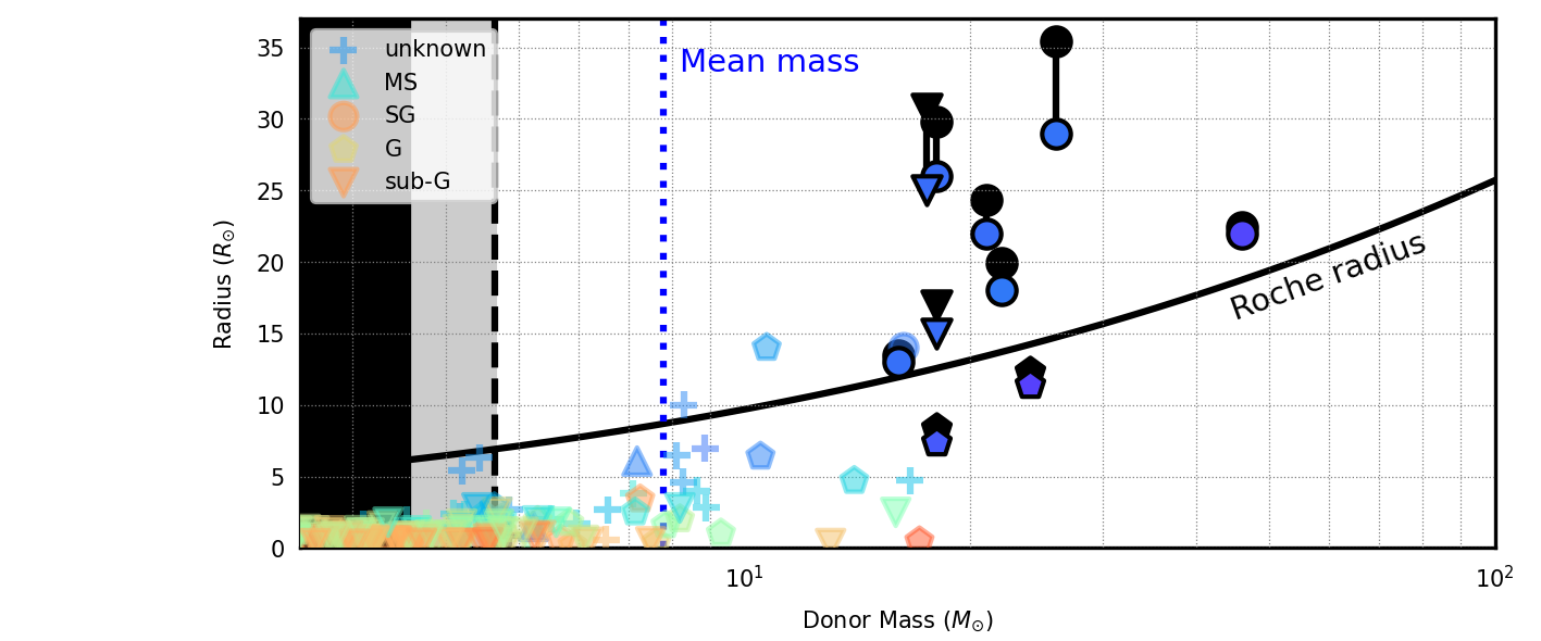
Figure 4: Roche Lobe radius in Eggleton approximation (Eggleton, 1983) versus mass for the donor star in M82 X-2. The donor has to lie around the black solid line in order to undergo Roche Lobe overflow. We overplot all donors from the HMXBs in Falanga et al. (2015) and all semidetached binary stars from Surkova & Svechnikov (2004) for comparison. For the HMXBs, we plot in black the Roche Lobe radius. Colors span the A (red)–O (blue) spectral types, and markers indicate different branches in the HR diagram. The grey shaded area is excluded by the absence of eclipses. The black area is prohibited by the mass function and the necessity that $\sin i\leq 1$.

With these constraints in mind (see Figure 4), and compared with known populations of donor stars in HMXBs, the most probable candidates are O/B giant stars between 5–100$M_{\odot}$. Between $\sim 17^{\circ}$ ($100\,M_{\odot}$ donor) and $\sim 60^{\circ}$ ($5\,M_{\odot}$ donor), we assume all orientations to be equally probable. This means that the values of the cosine of the inclination are equally probable between the two limiting cases $\cos 60^{\circ}$ and $\cos 17^{\circ}$. This gives an average inclination of $\sim 43^{\circ}$, corresponding to a donor mass of $\sim 7.8\,M_{\odot}$. Note that an archival search in HST data found several stars of this range of masses which could in principle be the donor (Heida et al., 2019).

Appendix E Magnetic field estimates

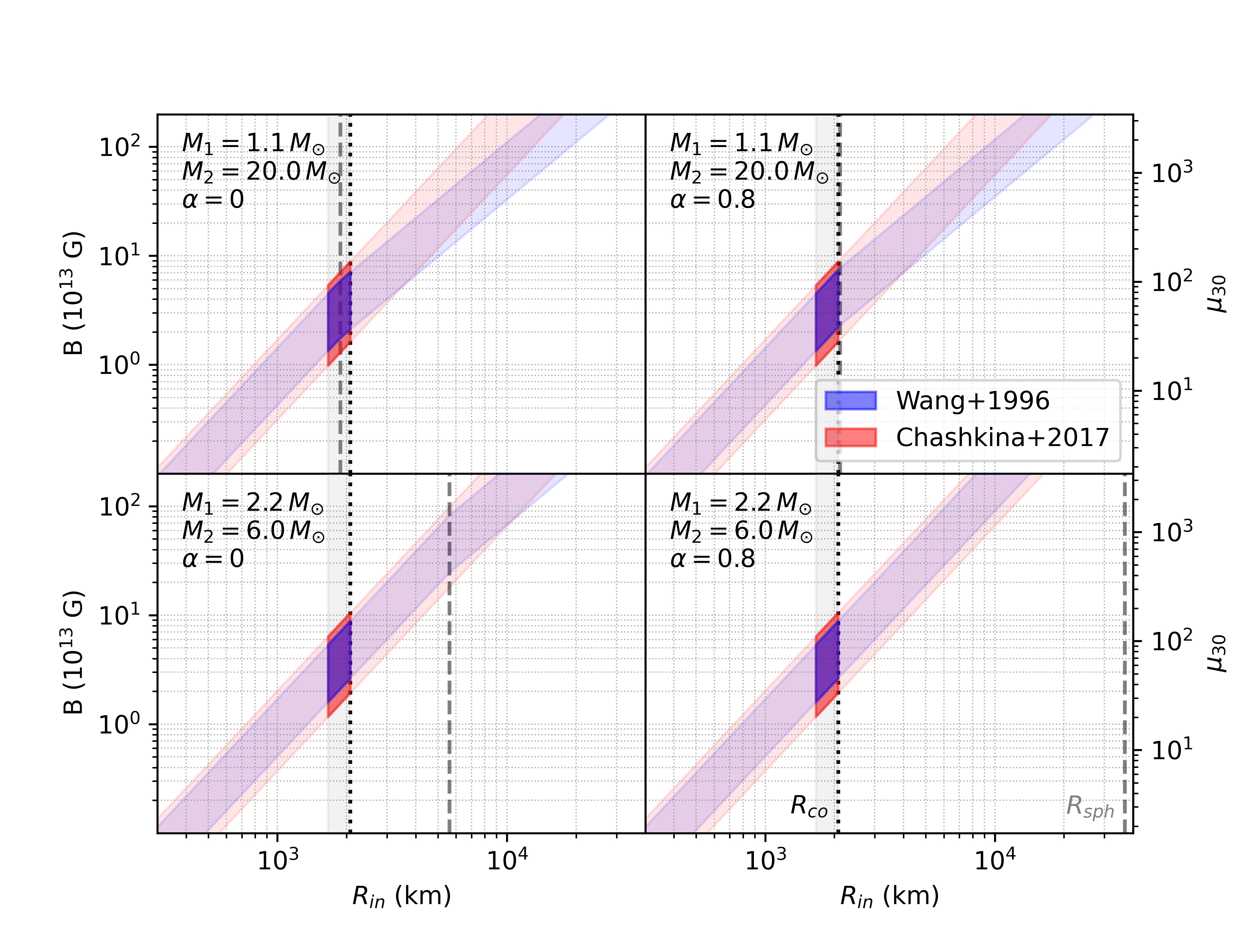
Figure 5: neutron star dipolar magnetic field estimate assuming spin equilibrium as described in the text, comparing the models from Wang (1996) (the area corresponds to values of $0.5<\xi<1$) and from Chashkina et al. (2017) (the area covers the range of viscosity parameter $0.01<\alpha_{v}<0.3$), in four cases with a range of mass ratios and a different mass loss fraction ($\alpha$ in Equation B3) from the donor. We show $R_{\rm co}$ and $R_{\rm sph}$ with vertical lines. Note that a lower mass ratio increases the estimated mass transfer. Also, the mass loss from the donor implies a larger mass transfer rate to justify the observed derivative. This explains the larger $R_{\rm sph}$. We highlight the region where $0.8<R_{\rm in}/R_{\rm co}<1$, as expected from spin equilibrium. For the traditional model we took into account a change of accretion rate due to mass loss inside $R_{\rm sph}$. The estimated dipolar magnetic field is always above $10^{13}$ G for reasonable values of the parameters.

Traditional models, such as those proposed by Ghosh & Lamb (1978) or Wang (1996), consider a thin disk with negligible radiation effects, and the inner radius is given by Equation C2. Therefore, given a mass accretion rate, the position of the inner radius in this model is a function of the dipolar component of the magnetic field, modulo the order-unity constant $\xi$. Since the source is close to spin equilibrium, as demonstrated by the spin behavior over time (see Table 1), the inner radius has to be close to the corotation radius. Therefore, equating the inner radius to the corotation radius, we can get an estimate of the magnetic field, as shown in Figure 5 with the blue band. Here, we take into account mass losses in a wind inside $R_{\rm sph}$, when relevant, until $R_{\rm in}$. We use the ”classical” mass loss obtained when the effects of advection are neglected (Shakura & Sunyaev, 1973). In this case, the accretion rate drops linearly with radius, and thus an upper limit on the accretion rate (i.e., an upper limit on the mass loss rate) corresponds to an upper limit on $R_{\rm in}$ and a lower limit to the magnetic field strength. Despite this conservative approach, the estimate on the magnetic field is robustly above $10^{13}$ G. Most models for sub-Eddington accretion agree within an order of magnitude for the treatment of spin equilibrium (see, e.g., Chen et al. 2021). However, it is possible that these models which are based on the interaction of a magnetized neutron star with a thin disk, with no radiation pressure either from the disk or from the central object, need to be corrected in the case of super-Eddington disks. Chashkina et al. (2017, 2019) have investigated this issue, finding that, indeed, the disk structure changes significantly when radiation pressure becomes dominant. In particular, they find that $\xi$ is not constant, but depends on local (inside the disk) and external (e.g. from the neutron star) radiation pressure, and the amount of advection in the disk. With the transfer rate $>100\times$Eddington we infer in this Paper, the inner radius becomes almost independent of the mass accretion rate and is described by Eq. 61 from Chashkina et al. (2017):

$$\frac{R_{\rm in}}{R_{g}}\approx{\left(\frac{73\alpha}{24}\right)}^{2/9}{\left[\lambda{\left(\frac{\mu}{10^{30}\mathrm{G\,cm^{3}}}\right)}^{2}\right]}^{2/9}$$ (E1)

where $\alpha\sim 0.1$ is the viscosity in the disk and $\lambda\sim 4\cdot 10^{10}\,(M_{p}/1.4M_{\odot})^{-5}$. Figure 5 shows that, for a reasonable range of the viscosity parameter $0.01<\alpha_{v}<0.3$, the estimate of the magnetic field obtained by equating the inner radius to the corotation radius using Equation E1 is similar to the prediction of traditional models using Equation C2, confirming an estimated magnetic field for M82 X-2 above $10^{13}$ G, as estimated with the classical model and by other authors in the literature (Tsygankov et al., 2016; Chen et al., 2021).

Appendix F Pulsed fraction in the XMM-Newton energy band

As opposed to many other PULXs, M82 X-2 is very difficult to study with XMM-Newton. Pulsations were not detected in many past observations of M82 X-2, despite the higher angular resolution of the EPIC-pn instrument. One of the reasons is the lack of pulsations below 3 keV, due to both an intrinsic low pulsed amplitude and the very strong emission of M82 X-1 and the M82 galaxy itself that increase the background at low energies. In the 2021 quasi-simultaneous observations with XMM-Newton and NuSTAR, we did manage to detect pulsations with EPIC-pn (Figure 6). M82 X-2 was observed by XMM-Newton on UT 2021-04-06 and 2021-04-16 for a total on-source exposure time of $\sim$70 ks. The only camera onboard XMM-Newton that is able to detect pulsations from M82 X-2 is EPIC-pn, that was set in Full Window mode.

We downloaded the data from the two observations from the XMM-Newton archive and processed them with the Science analysis software (SAS) version 20211130.

We ran the standard pipeline, using the tool epchain to obtain cleaned event files. The M82 field is very crowded, and it is not possible to separate the emission of M82 X-2, M82 X-1 and the diffuse Galactic center emission. However, being mostly interested in the timing properties of M82 X-2, a precise modeling of the background is not strictly needed. We selected photons coming from a region of $\sim 50^{\prime\prime}$ around the putative position of M82 X-2 We cleaned the data from periods of high background activity. Finally, we barycentered the data using the tool barycen using the Chandra position of M82 X-2, with the same ephemeris used in barycorr.

After this pre-processing, we folded the cleaned and barycentered event lists at the ephemeris obtained from the nearest NuSTAR observations, slightly adjusting the spin frequency through the maximization of the Rayleigh test. We calculated the pulsed fraction from a sinusoidal modeling of the pulsed profile, as (Max - Min) / (Max + Min). We plot this pulsed fraction, and the corresponding pulsed fraction from the quasi-simultaneous NuSTAR observations, in Figure 6

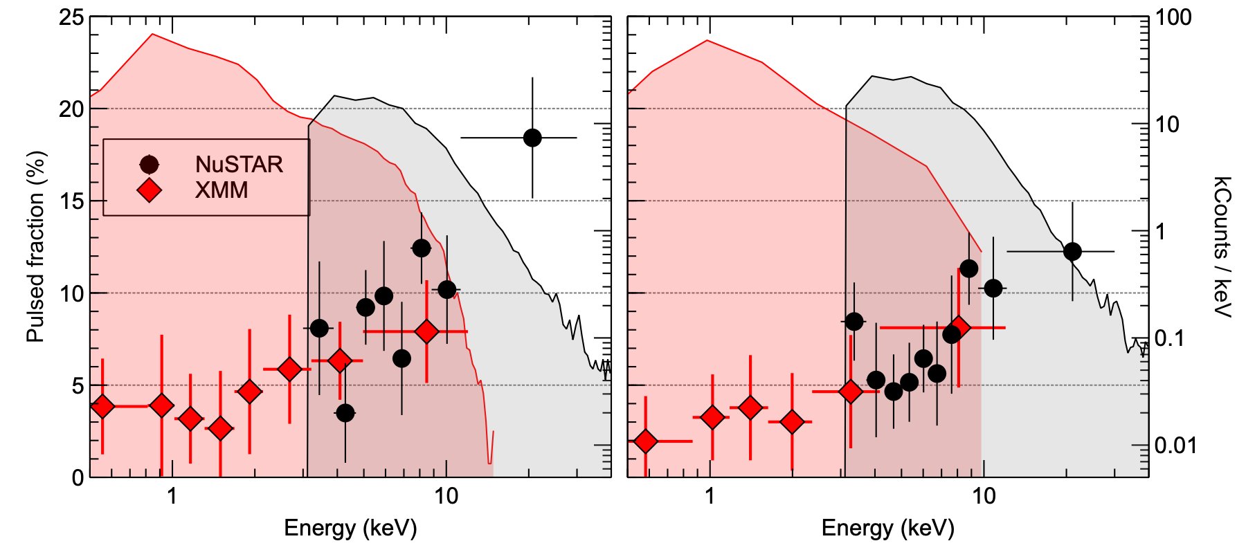
Figure 6: Pulsed amplitude versus energy, using XMM-Newton data from obsIDs 0870940101 and 0870940401, and NuSTAR data from obsIDs 30602027002 and 30602027004. We overplot the raw count spectra of NuSTAR and XMM, showing how XMM-Newton has many more counts, but in energy intervals with little or no pulsations.

References

- Abarca et al. (2021) Abarca, D., Parfrey, K., & Kluźniak, W. 2021, The Astrophysical Journal, 917, L31, doi: 10.3847/2041-8213/ac1859
- Astropy Collaboration et al. (2018) Astropy Collaboration, Price-Whelan, A. M., Sipőcz, B. M., et al. 2018, The Astronomical Journal, 156, 123, doi: 10.3847/1538-3881/aabc4f
- Bachetti (2018) Bachetti, M. 2018, Astrophysics Source Code Library, ascl:1805.019
- Bachetti et al. (2021) Bachetti, M., Pilia, M., Huppenkothen, D., et al. 2021, ApJ, 909, 33, doi: 10.3847/1538-4357/abda4a
- Bachetti et al. (2013) Bachetti, M., Rana, V., Walton, D. J., et al. 2013, ApJ, 778, 163, doi: 10.1088/0004-637X/778/2/163
- Bachetti et al. (2014) Bachetti, M., Harrison, F. A., Walton, D. J., et al. 2014, Nat., 514, 202, doi: 10.1038/nature13791
- Bachetti et al. (2020) Bachetti, M., Maccarone, T. J., Brightman, M., et al. 2020, ApJ, 891, 44, doi: 10.3847/1538-4357/ab6d00
- Barcons et al. (2017) Barcons, X., Barret, D., Decourchelle, A., et al. 2017, Astronomische Nachrichten, 338, 153, doi: 10.1002/asna.201713323
- Blundell et al. (2008) Blundell, K. M., Bowler, M. G., & Schmidtobreick, L. 2008, The Astrophysical Journal, 678, L47, doi: 10.1086/588027
- Brice et al. (2021) Brice, N., Zane, S., Turolla, R., & Wu, K. 2021, Monthly Notices of the Royal Astronomical Society, 504, 701, doi: 10.1093/mnras/stab915
- Brightman et al. (2019) Brightman, M., Harrison, F. A., Bachetti, M., et al. 2019, The Astrophysical Journal, 873, 115, doi: 10.3847/1538-4357/ab0215
- Buccheri et al. (1983) Buccheri, R., Bennett, K., Bignami, G. F., et al. 1983, A&A, 128, 245
- Chashkina et al. (2017) Chashkina, A., Abolmasov, P., & Poutanen, J. 2017, Monthly Notices of the Royal Astronomical Society, 470, 2799, doi: 10.1093/mnras/stx1372
- Chashkina et al. (2019) Chashkina, A., Lipunova, G., Abolmasov, P., & Poutanen, J. 2019, Astronomy and Astrophysics, 626, A18, doi: 10.1051/0004-6361/201834414
- Chen et al. (2021) Chen, X., Wang, W., & Tong, H. 2021, Journal of High Energy Astrophysics, 31, 1, doi: 10.1016/j.jheap.2021.04.002
- Cherepashchuk et al. (2021) Cherepashchuk, A. M., Belinski, A. A., Dodin, A. V., & Postnov, K. A. 2021, Monthly Notices of the Royal Astronomical Society, 507, L19, doi: 10.1093/mnrasl/slab083
- Chernov (2020) Chernov, S. V. 2020, Astron. Rep., 64, 425, doi: 10.1134/S1063772920050017
- Dall’Osso et al. (2015) Dall’Osso, S., Perna, R., & Stella, L. 2015, MNRAS, 449, 2144, doi: 10.1093/mnras/stv170
- D’Angelo & Spruit (2012) D’Angelo, C. R., & Spruit, H. C. 2012, Monthly Notices of the Royal Astronomical Society, 420, 416, doi: 10.1111/j.1365-2966.2011.20046.x
- Eggleton (1983) Eggleton, P. P. 1983, ApJ, 268, 368, doi: 10.1086/160960
- Ekşi et al. (2015) Ekşi, K. Y., Andaç, \. C., Çıkıntoğlu, S., et al. 2015, MNRAS Let., 448, L40, doi: 10.1093/mnrasl/slu199
- Erkut et al. (2020) Erkut, M. H., Türkoğlu, M. M., Ekşi, K. Y., & Alpar, M. A. 2020, The Astrophysical Journal, 899, 97, doi: 10.3847/1538-4357/aba61b
- Fabrika et al. (2006) Fabrika, S., Karpov, S., Abolmasov, P., Sholukhova, O., & Fabbiano, G. 2006, IAU, 230, 278, doi: 10.1017/S1743921306008441
- Fabrika et al. (2021) Fabrika, S. N., Atapin, K. E., Vinokurov, A. S., & Sholukhova, O. N. 2021, Astrophys. Bull., 76, 6, doi: 10.1134/S1990341321010077
- Falanga et al. (2015) Falanga, M., Bozzo, E., Lutovinov, A., et al. 2015, Astronomy and Astrophysics, 577, A130, doi: 10.1051/0004-6361/201425191
- Foreman-Mackey (2016) Foreman-Mackey, D. 2016, The Journal of Open Source Software, 1, 24, doi: 10.21105/joss.00024
- Foreman-Mackey et al. (2013) Foreman-Mackey, D., Hogg, D. W., Lang, D., & Goodman, J. 2013, PASP, 125, 306, doi: 10.1086/670067
- Frank et al. (2002) Frank, J., King, A., & Raine, D. J. 2002, Accretion Power in Astrophysics: Third Edition (Accretion Power in Astrophysics)
- Ghosh & Lamb (1978) Ghosh, P., & Lamb, F. K. 1978, ApJ, 223, L83, doi: 10.1086/182734
- Gladstone et al. (2009) Gladstone, J. C., Roberts, T. P., & Done, C. 2009, MNRAS, 397, 1836, doi: 10.1111/j.1365-2966.2009.15123.x
- Harris et al. (2020) Harris, C. R., Millman, K. J., van der Walt, S. J., et al. 2020, Nature, 585, 357, doi: 10.1038/s41586-020-2649-2
- Heida et al. (2019) Heida, M., Harrison, F. A., Brightman, M., et al. 2019, The Astrophysical Journal, 871, 231, doi: 10.3847/1538-4357/aafa77
- Hunter (2007) Hunter, J. D. 2007, Computing in Science & Engineering, 9, 90, doi: 10.1109/MCSE.2007.55
- Huppenkothen et al. (2016) Huppenkothen, D., Bachetti, M., Stevens, A. L., Migliari, S., & Balm, P. 2016, Astrophysics Source Code Library, ascl:1608.001
- Illarionov & Sunyaev (1975) Illarionov, A. F., & Sunyaev, R. A. 1975, A&A, 39, 185
- Israel et al. (2017) Israel, G. L., Belfiore, A., Stella, L., et al. 2017, Science, 355, 817, doi: 10.1126/science.aai8635
- Jiang et al. (2014) Jiang, Y.-F., Stone, J. M., & Davis, S. W. 2014, The Astrophysical Journal, 796, 106, doi: 10.1088/0004-637X/796/2/106
- Joss & Rappaport (1984) Joss, P. C., & Rappaport, S. A. 1984, Annual Review of Astronomy and Astrophysics, 22, 537, doi: 10.1146/annurev.aa.22.090184.002541
- Kaaret et al. (2017) Kaaret, P., Feng, H., & Roberts, T. P. 2017, Annual Review of Astronomy and Astrophysics, 55, 303, doi: 10.1146/annurev-astro-091916-055259
- Kelley et al. (1980) Kelley, R., Rappaport, S., & Petre, R. 1980, The Astrophysical Journal, 238, 699, doi: 10.1086/158026
- King & Lasota (2020) King, A., & Lasota, J.-P. 2020, Monthly Notices of the Royal Astronomical Society, 494, 3611, doi: 10.1093/mnras/staa930
- King et al. (2017) King, A., Lasota, J.-P., & Kluźniak, W. 2017, MNRAS Let., 468, L59, doi: 10.1093/mnrasl/slx020
- King (2008) King, A. R. 2008, MNRAS Let., 385, L113, doi: 10.1111/j.1745-3933.2008.00444.x
- Kosec et al. (2018) Kosec, P., Pinto, C., Walton, D. J., et al. 2018, Monthly Notices of the Royal Astronomical Society, 479, 3978, doi: 10.1093/mnras/sty1626
- Lam et al. (2015) Lam, S. K., Pitrou, A., & Seibert, S. 2015, in Proceedings of the Second Workshop on the LLVM Compiler Infrastructure in HPC, LLVM ’15 (New York, NY, USA: Association for Computing Machinery), doi: 10.1145/2833157.2833162
- Lange et al. (2001) Lange, C., Camilo, F., Wex, N., et al. 2001, MNRAS, 326, 274, doi: 10.1046/j.1365-8711.2001.04606.x
- Levine et al. (1993) Levine, A., Rappaport, S., Deeter, J. E., Boynton, P. E., & Nagase, F. 1993, ApJ, 410, 328, doi: 10.1086/172750
- Levine et al. (2000) Levine, A. M., Rappaport, S. A., & Zojcheski, G. 2000, ApJ, 541, 194, doi: 10.1086/309398
- Lu et al. (2022) Lu, W., Fuller, J., Quataert, E., & Bonnerot, C. 2022, arXiv e-prints, arXiv:2204.00847. https://arxiv.org/abs/2204.00847
- Luo et al. (2021) Luo, J., Ransom, S., Demorest, P., et al. 2021, The Astrophysical Journal, 911, 45, doi: 10.3847/1538-4357/abe62f
- Madsen et al. (2019) Madsen, K., Hickox, R., Bachetti, M., et al. 2019, 51, 166
- Mellah et al. (2019) Mellah, I. E., Sundqvist, J. O., & Keppens, R. 2019, A&A, 622, L3, doi: 10.1051/0004-6361/201834543
- Middleton et al. (2022) Middleton, M. J., Higginbottom, N., Knigge, C., Khan, N., & Wiktorowicz, G. 2022, Monthly Notices of the Royal Astronomical Society, 509, 1119, doi: 10.1093/mnras/stab2991
- Middleton et al. (2021) Middleton, M. J., Walton, D. J., Alston, W., et al. 2021, Monthly Notices of the Royal Astronomical Society, 506, 1045, doi: 10.1093/mnras/stab1280
- Misra et al. (2020) Misra, D., Fragos, T., Tauris, T. M., Zapartas, E., & Aguilera-Dena, D. R. 2020, Astronomy and Astrophysics, 642, A174, doi: 10.1051/0004-6361/202038070
- Mushtukov et al. (2017) Mushtukov, A. A., Suleimanov, V. F., Tsygankov, S. S., & Ingram, A. 2017, Monthly Notices of the Royal Astronomical Society, 467, 1202, doi: 10.1093/mnras/stx141
- Mushtukov et al. (2015) Mushtukov, A. A., Suleimanov, V. F., Tsygankov, S. S., & Poutanen, J. 2015, MNRAS, 454, 2539, doi: 10.1093/mnras/stv2087
- Pinto et al. (2016) Pinto, C., Fabian, A., Middleton, M., & Walton, D. 2016, arXiv, arXiv:1611.00623. https://arxiv.org/abs/1611.00623
- Pletsch & Clark (2015) Pletsch, H. J., & Clark, C. J. 2015, The Astrophysical Journal, 807, 18, doi: 10.1088/0004-637X/807/1/18
- Poutanen et al. (2007) Poutanen, J., Lipunova, G., Fabrika, S., Butkevich, A. G., & Abolmasov, P. 2007, MNRAS, 377, 1187, doi: 10.1111/j.1365-2966.2007.11668.x
- Ray et al. (2018) Ray, P. S., Arzoumanian, Z., Brandt, S., et al. 2018, Space Telescopes and Instrumentation 2018: Ultraviolet to Gamma Ray, 10699, 1069919, doi: 10.1117/12.2312257
- Rodríguez Castillo et al. (2020) Rodríguez Castillo, G. A., Israel, G. L., Belfiore, A., et al. 2020, The Astrophysical Journal, 895, 60, doi: 10.3847/1538-4357/ab8a44
- Romanova et al. (2004) Romanova, M. M., Ustyugova, G. V., Koldoba, A. V., & Lovelace, R. V. E. 2004, ApJ, 616, L151, doi: 10.1086/426586
- Shakura & Sunyaev (1973) Shakura, N. I., & Sunyaev, R. A. 1973, A&A, 24, 337
- Soberman et al. (1997) Soberman, G. E., Phinney, E. S., & van den Heuvel, E. P. J. 1997, Astronomy and Astrophysics, v.327, p.620-635, 327, 620
- Stoyanov & Zamanov (2009) Stoyanov, K. A., & Zamanov, R. K. 2009, Astronomische Nachrichten, 330, 727, doi: 10.1002/asna.200811224
- Surkova & Svechnikov (2004) Surkova, L. P., & Svechnikov, M. A. 2004, VizieR Online Data Catalog
- Tauris & Savonije (2001) Tauris, T. M., & Savonije, G. J. 2001, Spin-Orbit Coupling in X-Ray Binaries, Vol. 567 (eprint: arXiv:astro-ph/0001014), 337
- Tauris & van den Heuvel (2006) Tauris, T. M., & van den Heuvel, E. P. J. 2006, Compact stellar X-ray sources, 623
- Tsygankov et al. (2016) Tsygankov, S. S., Mushtukov, A. A., Suleimanov, V. F., & Poutanen, J. 2016, MNRAS, 457, 1101, doi: 10.1093/mnras/stw046
- van den Heuvel (1994) van den Heuvel, E. P. J. 1994, Interacting Binaries: Topics in Close Binary Evolution., 263–474
- Vasilopoulos et al. (2021) Vasilopoulos, G., Koliopanos, F., Haberl, F., et al. 2021, The Astrophysical Journal, 909, 50, doi: 10.3847/1538-4357/abda49
- Virtanen et al. (2020) Virtanen, P., Gommers, R., Oliphant, T. E., et al. 2020, Nature Methods, 17, 261, doi: 10.1038/s41592-019-0686-2
- Walton et al. (2016) Walton, D. J., Tomsick, J. A., Madsen, K. K., et al. 2016, The Astrophysical Journal, 826, 87, doi: 10.3847/0004-637X/826/1/87
- Wang (1996) Wang, Y.-M. 1996, The Astrophysical Journal, 465, L111, doi: 10.1086/310150
- Xu & Li (2017) Xu, K., & Li, X.-D. 2017, The Astrophysical Journal, 838, 98, doi: 10.3847/1538-4357/aa65d5
- Zhang et al. (2016) Zhang, S. N., Feroci, M., Santangelo, A., et al. 2016, arXiv:1607.08823 [astro-ph], 99051Q, doi: 10.1117/12.2232034