Non-splitting Neyman-Pearson Classifiers

Abstract

The Neyman-Pearson (NP) binary classification paradigm constrains the more severe type of error (e.g., the type I error) under a preferred level while minimizing the other (e.g., the type II error). This paradigm is suitable for applications such as severe disease diagnosis, fraud detection, among others. A series of NP classifiers have been developed to guarantee the type I error control with high probability. However, these existing classifiers involve a sample splitting step: a mixture of class 0 and class 1 observations to construct a scoring function and some left-out class 0 observations to construct a threshold. This splitting enables classifier construction built upon independence, but it amounts to insufficient use of data for training and a potentially higher type II error. Leveraging a canonical linear discriminant analysis (LDA) model, we derive a quantitative CLT for a certain functional of quadratic forms of the inverse of sample and population covariance matrices, and based on this result, develop for the first time NP classifiers without splitting the training sample. Numerical experiments have confirmed the advantages of our new non-splitting parametric strategy.

Keywords: classification, Neyman-Pearson (NP), type I error, non-splitting, efficiency.

1 Introduction

Classification aims to accurately assign class labels (e.g., fraud vs. non-fraud) to new observations (e.g., new credit card transactions) on the basis of labeled observations (e.g., labeled transactions). The prediction is usually not perfect. In transaction fraud detection, two errors might arise: (1) mislabeling a fraudulent transaction as non-fraudulent and (2) mislabeling a non-fraudulent transaction as fraudulent. The consequences of the two errors are different: while declining a legitimate transaction may cause temporary inconvenience for a consumer, approving a fraudulent transaction can result in a substantial financial loss for a credit card company. In severe disease diagnosis (e.g., cancer vs. normal), the asymmetry of the two errors’ importance is even greater: while misidentifying a healthy person as ill may cause anxiety and create additional medical expenses, telling cancer patients that they are healthy may cost their lives. In these applications, it is critical to prioritize the control of the more important error.

Most theoretical work on binary classification concerns risk. Risk is a weighted sum of type I error (i.e., the conditional probability that the predicted label is $1$ given that the true label is $0$) and type II error (i.e., the conditional probability that the predicted label is $0$ given that the true label is $1$), where the weights are marginal probabilities of the two class labels. In the context of transaction fraud detection, coding the fraud class as $0$, we would like to control type I error under some small level. The common classical paradigm, which minimizes the risk, does not guarantee delivery of classifiers that have type I error bounded by the preferred level. To address this concern, we can employ a general statistical framework for controlling asymmetric errors in binary classification: the Neyman-Pearson (NP) classification paradigm, which seeks a classifier that minimizes type II error subject to type I error $\leq$ $\alpha$, where $\alpha$ is a user-specified level, usually a small value (e.g., $5\%$ ). The NP framework can achieve the best type II error given a high priority on the type I error.

The NP approach is fundamental in hypothesis testing (justified by the NP lemma), but its use in classification did not occur until the 21st century (Cannon et al., 2002; Scott and Nowak, 2005). In the past ten years, there is significant progress in the theoretical/methodological investigation of NP classification. An incomplete overview includes (i) a theoretical evaluation criterion for NP classifiers: the NP oracle inequalities (Rigollet and Tong, 2011), (ii) classifiers satisfying this criterion under different settings (Tong, 2013; Zhao et al., 2016; Tong et al., 2020), and (iii) practical algorithms for constructing NP classifiers (Tong et al., 2018, 2020), (iv) generalizations to domain adaptation (Scott, 2019) and to multi-class (Tian and Feng, 2021).

Unlike the oracle classifier under the classical paradigm, which thresholds the regression function at precisely $1/2$, the threshold of the NP oracle is $\alpha$-dependent and needs to be estimated when we construct sample-based classifiers. Threshold determination is the key in NP classification algorithms, because it is subtle to ensure a high probability control on the type I error under $\alpha$ while achieving satisfactory type II error performance.

For existing NP classification algorithms (Tong, 2013; Zhao et al., 2016; Tong et al., 2018, 2020), a sample splitting step is common practice: a mixture of class 0 and class 1 observations to construct a scoring function $\hat{s}(\cdot)$ (e.g., fitted sigmoid function in logistic regression) and some left-out class 0 observations $\{x^{0}_{1},\cdots,x^{0}_{m}\}$ to construct a threshold. Then under proper sampling assumptions, conditioning on $\hat{s}(\cdot)$, the set $\{s_{1}:=\hat{s}(x^{0}_{1}),\cdots,s_{m}:=\hat{s}(x^{0}_{m})\}$ consists of independent elements. This independence is important in the subsequent threshold determination and classifier construction. Let us take the NP umbrella algorithm (Tong et al., 2018) as an example: it constructs an NP classifier $\hat{\varphi}_{\alpha}(\cdot)={\rm 1}\kern-2.40005pt{\rm I}(\hat{s}(\cdot)>s_{(k^{*})})$, where ${\rm 1}\kern-2.40005pt{\rm I}(\cdot)$ is the indicator function, $s_{(k^{*})}$ is the $k^{*}$th order statistic in $\{s_{1},\cdots,s_{m}\}$ and $k^{*}=\min\left\{k\in\{1,\cdots,m\}:\sum_{i=k}^{m}{m\choose j}(1-\alpha)^{j}\alpha^{m-j}\leq\delta\right\}$. The smallest order was chosen to have the best type II error. The type I error violation rate has been shown to satisfy ${\rm I}\kern-1.79993pt{\rm P}(R_{0}(\hat{\varphi}_{\alpha})>\alpha)\leq\sum_{i=k}^{m}{m\choose j}(1-\alpha)^{j}\alpha^{m-j}$, where $R_{0}$ denotes the (population-level) type I error. Hence with probability at least $1-\delta$, we have $R_{0}(\hat{\varphi}_{\alpha})\leq\alpha$. Without the independence of $\{s_{1},\cdots,s_{m}\}$, the upper bound on the violation rate does not hold. Therefore, if we used up all class 0 observations in constructing $\hat{s}(\cdot)$, this umbrella algorithm fails. In other NP works (Tong, 2013; Zhao et al., 2016; Tong et al., 2020), the independence is necessary in threshold determination when applying Vapnik-Chervonenkis inequality, Dvoretzky-Kiefer-Wolfowitz inequality, or constructing classic t-statistics, respectively.

In general, setting aside part of class 0 sample lowers the quality of the scoring function $\hat{s}(\cdot)$, and therefore makes the type II error deteriorate. This becomes a serious concern when the class 0 sample size is small. A more data-efficient alternative is to use all data to construct the scoring function, but this would lose the critical independence property when constructing the threshold. Innovating a non-splitting strategy has long been in the “wish list.” This is an important but challenging task. For example, the NP umbrella algorithm, which has no assumption on data distribution and adapts all scoring-type classification methods (e.g., logistic regression, neural nets) to the NP paradigm universally via the non-parametric order statistics approach, has little potential to be extended to the non-splitting scenario, simply because there is no way to characterize the general dependence. To address it, we need to start from tractable distributional assumptions.

Among the commonly used models for classification is the linear discriminant analysis (LDA) model (Hastie et al., 2009; James et al., 2014; Fan et al., 2020), which assumes that the two class-conditional feature distributions are Gaussian with different means but a common covariance matrix: $\mathcal{N}(\bm{\mu}^{0},\Sigma)$ and $\mathcal{N}(\bm{\mu}^{1},\Sigma)$. Classifiers based on the LDA model have been popular in the literature (Shao et al., 2011; Fan et al., 2012; Witten and Tibshirani, 2012; Mai et al., 2012; Hao et al., 2015; Pan et al., 2016; Wang and Jiang, 2018; Cai and Zhang, 2019; Li and Lei, 2018; Sifaou et al., 2020). Hence, it is natural to start our inquiry with the LDA model. However, even this canonical model demands novel intermediate technical results that were not available in the literature. For example, we will need delicate expansion results of quadratic forms of the inverse of sample and population covariance matrices, which we establish for the first time in this manuscript.

As the first effort to investigate a non-splitting strategy under the NP paradigm, this work addresses basic settings. We only work in the regime that $p/n\rightarrow[0,1)$, where $p$ is the feature dimensionality and $n$ is the sample size. We take minimum assumptions on $\Sigma$ and $\bm{\mu}_{d}:=\bm{\mu}^{1}-\bm{\mu}^{0}$: $\bm{\mu}_{d}^{\top}\Sigma^{-1}\bm{\mu}_{d}$ is bounded from below. We do not have specific structural assumptions on $\Sigma$ or $\bm{\mu}_{d}$ such as sparsity. With these minimal assumptions, we propose our new classifier eLDA (where e stands for data efficiency) based on a quantitative CLT for a certain functional of quadratic forms of the inverse of sample and population covariance matrices and show that eLDA respects the type I error control with high probability. Moreover, if $p/n\rightarrow 0$, the excess type II error of eLDA, that is the difference between the type II error of eLDA and that of the NP oracle, diminishes as the sample size increases; if $p/n\rightarrow r_{0}\in(0,1)$, the excess type II error of eLDA diminishes if and only if ${\bm{\mu}}_{d}^{\top}\Sigma^{-1}{\bm{\mu}}_{d}$ diverges. We note in particular that this work is the first one to establish lower bound results on excess type II error under the NP paradigm.

Table 1: eLDA vs. pNP-LDA.

	eLDA	pNP-LDA
type I error	.0314	.0037
type II error	.4478	.7638

In addition to enjoying good theoretical properties, eLDA has numerical advantages. Here we take a toy example: $\Sigma=I$, $\bm{\mu}_{d}=(1.2,1.2,1.2)^{\top}$ and $\bm{\mu}^{0}=(0,0,0)^{\top}$. The sample sizes $n_{0}$ and $n_{1}$ for classes 0 and 1 respectively are both 50. We set the type I error upper bound $\alpha=0.05$ and the type I error violation rate target $\delta=0.1$. In this situation, if we were to use the NP umbrella algorithm, we would have to reserve at least 45 (i.e., $\lceil\log\delta/\log(1-\alpha)\rceil$) class 0 observations for threshold determination, and thus at most 5 class 0 observations can be used for scoring function training. This is obviously undesirable. So we only compare the newly proposed eLDA with pNP-LDA, another LDA based classifier proposed in Tong et al. (2020) with sample splitting, whose threshold determination explicitly relies on the parametric assumption. In Table 1, the type I error and type II error were averaged over $1{,}000$ repetitions and evaluated on a very large test set ($50{,}000$ observations from each class) that approximates the population. The result shows that our new non-splitting eLDA classifier clearly outperforms the splitting pNP-LDA classifier by having a much smaller type II error. This example is not a coincidence. When the more generic nonparametric NP umbrella algorithm does not apply (or does not work well) due to sample size limitations, eLDA usually dominates pNP-LDA.

The rest of the paper is organized as follows. In Section 2, we introduce the essential notations and assumptions. In Section 3, we derive the efficient non-splitting NP classifier eLDA and its close relative $\verb+feLDA+$, where f stands for fixed feature dimension, and show their main theoretical results. Technical preliminaries are presented in Section 4, followed by the proof of the main theorem in Section 5. In Section 6, we present simulation and real data studies. We provide a short discussion in Section 7. In addition, in Appendix A, we give further remark on our assumptions. The proofs of other theoretical results except for the main theorem are postponed to Appendix B. In Appendix C, we provide the proofs of the technical preliminaries in Section 4, followed by the proofs of the key lemmas in the proof of the main theorem in Appendix D. Finally, Appendix E collects additional numerical results.

2 Model and Setups

Let $\phi:\mathcal{X}\subset\mathbb{R}^{p}\to\{0,1\}$ denote a mapping from the feature space to the label space. The level-$\alpha$ NP oracle $\phi_{\alpha}^{*}(\cdot)$ is defined as the solution to the program $\min_{R_{0}(\phi)\leq\alpha}R_{1}(\phi),$ where $R_{0}(\phi)={\rm I}\kern-1.79993pt{\rm P}\{\phi({\bf x})\neq Y\big{|}Y=0\}$ and $R_{1}(\phi)={\rm I}\kern-1.79993pt{\rm P}\{\phi({\bf x})\neq Y\big{|}Y=1\}$ denote the (population-level) type I and type II errors of $\phi(\cdot)$, respectively. We assume the linear discriminant analysis (LDA) model, i.e., $({\bf x}|Y=0)\sim\mathcal{N}({\bm{\mu}}^{0},\Sigma)$ and $({\bf x}|Y=1)\sim\mathcal{N}({\bm{\mu}}^{1},\Sigma)$, where ${\bm{\mu}}^{0},{\bm{\mu}}^{1}\in\mathbb{R}^{p}$ and the common positive definite covariance matrix $\Sigma\in\mathbb{R}^{p\times p}$. Under the LDA model, the level-$\alpha$ NP oracle classifier can be derived explicitly as

$$\phi_{\alpha}^{*}(x)={\rm 1}\kern-2.40005pt{\rm I}\Big{(}(\Sigma^{-1}{\bm{\mu}}_{d})^{\top}x>\sqrt{{\bm{\mu}}_{d}^{\top}\Sigma^{-1}{\bm{\mu}}_{d}}\,\Phi^{-1}(1-\alpha)+{\bm{\mu}}_{d}^{\top}\Sigma^{-1}{\bm{\mu}}^{0}\Big{)}\,,$$ (2.1)

in which ${\bm{\mu}}_{d}={\bm{\mu}}^{1}-{\bm{\mu}}^{0}$, and $\Phi^{-1}(1-\alpha)$ denotes the $(1-\alpha)$-th quantile of standard normal distribution.

For readers’ convenience, we introduce a few notations together. For any $k\in\mathbb{N}$, let $I_{k}$ denote the identity matrix of size $k$, ${\bf{1}}_{k}$ denote the all-one column vector of dimension $k$. For arbitrary two column vectors ${\bf u},{\bf v}$ of dimensions $a,b$, respectively, and any $a\times b$ matrix $M$, we write $(M)_{{\bf u}{\bf v}}$ as the quadratic form ${\bf u}^{\top}M{\bf v}$. Moreover, we write $M_{ij}$ or $(M)_{ij}$ for $i\in\{1,\cdots,a\}$ and $j\in\{1,\cdots,b\}$ as the $(i,j)$-th entry of $M$. We use $\|A\|$ to denote the operator norm for a matrix $A$ and use $\|\mathbf{v}\|$ to denote the $\ell_{2}$ norm of a vector $\mathbf{v}$. For two positive sequences $A_{n}$ and $B_{n}$, we adopt the notation $A_{n}\asymp B_{n}$ to denote $C^{-1}A_{n}\leq B_{n}\leq CA_{n}$ for some constant $C>1$. We will use $c$ or $C$ to represent a generic positive constant which may vary from line to line.

In the methodology and theory development, we assume that we have access to i.i.d. observations from class 0, $\mathcal{S}^{0}=\{X^{0}_{1},\cdots,X^{0}_{n_{0}}\}$, and i.i.d. observations from class 1, $\mathcal{S}^{1}=\{X^{1}_{1},\cdots,X^{1}_{n_{1}}\}$, where the sample sizes $n_{0}$ and $n_{1}$ are non-random positive integers. Moreover, the observations in $\mathcal{S}^{0}$ and $\mathcal{S}^{1}$ are independent. We also assume the following assumption unless specified otherwise.

Assumption 1.

(i) (On feature dimensionality and sample sizes): the dimension of features $p$ and the sample sizes of the two classes $n_{0},n_{1}$ satisfy $n_{0}/n>c_{0},n_{1}/n>c_{1}$ for some positive constants $c_{0}$ and $c_{1}$, and

$$r\equiv r_{n}:=p/n\to r_{0}\in[0,1)$$

as the sample size $n=n_{0}+n_{1}\to\infty$.
(ii) (On Mahalanobis distance): we assume that

$$\varDelta_{d}:={\bm{\mu}}_{d}^{\top}\Sigma^{-1}{\bm{\mu}}_{d}\geq c_{2}$$ (2.2)

for some positive constant $c_{2}>0$.

Assumption 1 is quite natural and almost minimal to the LDA model about $\Sigma$, ${\bm{\mu}}^{0}$, and ${\bm{\mu}}^{1}$. First, our theory strongly depends on the analysis of population and sample covariance matrices. To make the inverse sample covariance matrix $\widehat{\Sigma}^{-1}$ well-defined, we have to restrict the ratio $p/n$ strictly smaller than $1$. Moreover, the sample size for either class needs to be comparable to the total sample size; otherwise, the class with a negligible sample size would be treated as noises. Second, since the Mahalanobis distance characterizes the difference between the two classes, we adopt the common regularity condition in the literature that it is bounded from below by some positive constant.

To create a sample-based classifier, the most straightforward strategy is to replace the unknown parameters in (2.1) with their sample counterparts. However, this strategy is not appropriate for our inquiry for two reasons: (i) it is well-known that direct substitutions can result in inaccurate estimates when $p/n\to r_{0}\in(0,1)$; (ii) we aim for a high probability control on the type I error of the constructed classifier, and for that goal, a naive plug-in will not even work for fixed feature dimensionality. These two concerns demand that delicate refinements and corrections be made to the sample counterparts.

Before diving into the classifier construction in the next section, we introduce the notations for sample covariance matrix $\widehat{\Sigma}$ and sample mean vectors $\hat{\bm{\mu}}^{a}$, $a=1,2$, and express them in forms that are more amenable in our analysis. Recall that

$$\widehat{\Sigma}=\frac{1}{n_{0}+n_{1}-2}\sum_{a=0,1}\sum_{i=1}^{n_{a}}(X^{a}_{i}-\hat{\bm{\mu}}^{a})(X^{a}_{i}-\hat{\bm{\mu}}^{a})^{\top}\,,\quad\hat{\bm{\mu}}^{a}=\frac{1}{n_{a}}\left(X^{a}_{1}+\ldots+X^{a}_{n_{a}}\right)\,,\quad a=0,1\,.$$

We set the $p$ by $n$ data matrix by ${X}=(x_{ij})_{p,n}:=({X}^{0},{X}^{1})$, where

$${{X}}^{a}:=\frac{1}{(np)^{1/4}}\Sigma^{-\frac{1}{2}}(X_{1}^{a}-{\bm{\mu}}^{a},\cdots,X_{n_{a}}^{a}-{\bm{\mu}}^{a}),\quad a=0,1\,.$$

Note that all entries in the $p\times n$ matrix ${X}$ are i.i.d. Gaussian with mean $0$ and variance $1/\sqrt{np}$. The scaling ${1}/{(np)^{1/4}}$ is to ensure that the spectrum of $XX^{\top}$ has asymptotically a fixed diameter, making it a convenient choice for technical derivations. We define two unit column vectors of dimension $n$:

$${\bf{e}}_{0}:=\frac{1}{\sqrt{n_{0}}}({\bf{1}}_{n_{0}}^{\top},0,\cdots,0)^{\top}\,,\quad{\bf{e}}_{1}:=\frac{1}{\sqrt{n_{1}}}(0,\cdots,0,{\bf{1}}_{n_{1}}^{\top})^{\top}\,.$$ (2.3)

With the above notations, we can rewrite the sample covariance matrix $\widehat{\Sigma}$ as

$$\widehat{\Sigma}=\frac{\sqrt{np}}{n-2}\Sigma^{\frac{1}{2}}{{X}}\Big{(}I_{n}-{{E}}{{E}}^{\top}\Big{)}{{X}}^{\top}\Sigma^{\frac{1}{2}}\,,\text{ where }E:=({\bf{e}}_{0},{\bf{e}}_{1})\,.$$ (2.4)

For the sample means, we can rewrite them as

$$\hat{\bm{\mu}}^{a}=\sqrt{\frac{n}{n_{a}}}\,r^{\frac{1}{4}}\Sigma^{\frac{1}{2}}{X}{\bf e}_{a}+{\bm{\mu}}^{a}\,,\qquad a=0,1\,.$$ (2.5)

Furthermore, we write the sample mean difference vector as

$$\hat{\bm{\mu}}_{d}:=\hat{\bm{\mu}}^{1}-\hat{\bm{\mu}}^{0}=r^{\frac{1}{4}}\Sigma^{\frac{1}{2}}{X}{\bf v}_{1}+{\bm{\mu}}_{d}\,,\qquad\text{where }{\bf{v}_{1}}:=\begin{pmatrix}-\frac{\sqrt{n}}{{n_{0}}}{\bf 1}_{n_{0}}\\ \frac{\sqrt{n}}{{n_{1}}}{\bf 1}_{n_{1}}\end{pmatrix}=-\sqrt{\frac{n}{n_{0}}}{\bf e}_{0}+\sqrt{\frac{n}{n_{1}}}{\bf e}_{1}\,.$$ (2.6)

3 New Classifiers and Main Theoretical Results

In this section, we propose our new NP classifier eLDA and establish its theoretical properties regarding type I and type II errors. We also construct a variant classifier feLDA for fixed feature dimensions.

To motivate the construction of eLDA, we introduce an intermediate level-$\alpha$ NP oracle

$$\tilde{\phi}_{\alpha}^{*}(x)={\rm 1}\kern-2.40005pt{\rm I}\Big{(}\widehat{A}^{\top}x>\sqrt{\widehat{A}^{\top}\Sigma\widehat{A}}\,\Phi^{-1}(1-\alpha)+\widehat{A}^{\top}{\bm{\mu}}^{0}\Big{)}\,,$$ (3.1)

where $\widehat{A}=\widehat{\Sigma}^{-1}\hat{\bm{\mu}}_{d}$ is a shorthand notation we will frequently use in this manuscript. One can easily deduce that the type I error of $\tilde{\phi}_{\alpha}^{*}(\cdot)$ in (3.1) is exactly $\alpha$. Note that $\tilde{\phi}_{\alpha}^{*}(\cdot)$ involves unknown parameters $\Sigma$ and ${\bm{\mu}}^{0}$, so it is not a sample-based classifier. However, it is still of interest to compare the type II error of $\tilde{\phi}_{\alpha}^{*}(\cdot)$ to that of the level-$\alpha$ NP oracle in (2.1).

Lemma 1.

Let $\tilde{\phi}_{\alpha}^{*}(\cdot)$ be defined in (3.1). Under Assumption 1, the type I error of $\tilde{\phi}_{\alpha}^{*}(\cdot)$ is exactly $\alpha$, i.e., $R_{0}(\tilde{\phi}_{\alpha}^{*}\,)=\alpha\,$. Further if $r=p/n\to 0$, then for any $\varepsilon\in(0,1/2)$ and $D>0$, when $n>n(\varepsilon,D)$, we have with probability at least $1-n^{-D}$ , the type II error satisfies

$$R_{1}(\tilde{\phi}_{\alpha}^{*}\,)-R_{1}({\phi}_{\alpha}^{*}\,)\leq C\Big{(}r+n^{-\frac{1}{2}+\varepsilon}\Big{)}\sqrt{\varDelta_{d}}\,\exp\Big{(}-\frac{c\varDelta_{d}}{2}\Big{)}\,$$

for some constants $C,c>0$, where $C$ may depend on $c_{0,1,2}$ and $\alpha$, and $\varDelta_{d}$ is defined in (2.2).

Lemma 1 indicates that $R_{1}(\tilde{\phi}_{\alpha}^{*})-R_{1}({\phi}_{\alpha}^{*})$ goes to 0 under Assumption 1 and $p/n\to 0$. This prompts us to construct a fully sample-based classifier by modifying the unknown parts of $\tilde{\phi}_{\alpha}^{*}(\cdot)$. Towards that, we denote the threshold of $\widehat{A}^{\top}x$ in $\tilde{\phi}_{\alpha}^{*}(\cdot)$ by

$$F(\Sigma,{\bm{\mu}}^{0}):=\sqrt{\widehat{A}^{\top}\Sigma\widehat{A}}\,\Phi^{-1}(1-\alpha)+\widehat{A}^{\top}{\bm{\mu}}^{0}\,,$$ (3.2)

and denote a sample-based estimate of $F(\Sigma,{\bm{\mu}}^{0})$ by $\widehat{F}(\widehat{\Sigma},\hat{\bm{\mu}}^{0})$, whose exact form will be introduced shortly. By studying the difference between $F(\Sigma,{\bm{\mu}}^{0})$ and $\widehat{F}(\widehat{\Sigma},\hat{\bm{\mu}}^{0})$, we will construct a statistic $\widehat{C}_{\alpha}^{p}$ based on $\widehat{F}(\widehat{\Sigma},\hat{\bm{\mu}}^{0})$ (where the superscript $p$ stands for parametric) that is slightly larger than $F(\Sigma,{\bm{\mu}}^{0})$ with high probability. The proposed classifier eLDA will then be defined by replacing $F(\Sigma,{\bm{\mu}}^{0})$ in (3.1) with $\widehat{C}_{\alpha}^{p}$.

Concretely, suppose we hope that the probability of type I error of eLDA no larger than $\alpha$ is at least around $1-\delta$, for some small given constant $\delta\in(0,1)$. We define

$$\widehat{F}(\widehat{\Sigma},\hat{\bm{\mu}}^{0}):=\frac{\sqrt{\widehat{A}^{\top}\widehat{\Sigma}\widehat{A}}}{1-r}\,\Phi^{-1}(1-\alpha)+\widehat{A}^{\top}\hat{\bm{\mu}}^{0}-\sqrt{\frac{n}{n_{0}}}\frac{r}{1-r}{\bf v}_{1}^{\top}{\bf e}_{0}\,,$$ (3.3)

$$\widehat{C}_{\alpha}^{p}:=\widehat{F}(\widehat{\Sigma},\hat{\bm{\mu}}^{0})+\sqrt{\frac{\big{(}(1-r)\widehat{A}^{\top}\widehat{\Sigma}\widehat{A}-r\|{\bf v}_{1}\|^{2}\big{)}\widehat{V}}{n}}\,\Phi^{-1}(1-\delta)\,,$$ (3.4)

in which $\widehat{V}=\sum_{i=1}^{3}\widehat{V}_{i}$ and

$$\widehat{V}_{1}:=\big{(}(1-r)\widehat{A}^{\top}\widehat{\Sigma}\widehat{A}-r\|{\bf v}_{1}\|^{2}\big{)}\mathsf{C}^{2}\Phi_{\alpha}^{2}\frac{2(1+r)}{(1-r)^{7}}\,,$$

$$\widehat{V}_{2}:=\mathsf{C}^{2}\Phi_{\alpha}^{2}\|{\bf v}_{1}\|^{2}\,\frac{4r(1+r)}{(1-r)^{7}}+\frac{n}{n_{0}(1-r)^{3}}+2\mathsf{C}\Phi_{\alpha}\|{\bf v}_{1}\|\,\sqrt{\frac{n_{1}}{n_{0}}}\,\frac{2r}{(1-r)^{5}}\,,$$

$$\widehat{V}_{3}:=\frac{\|{\bf v}_{1}\|^{2}}{(1-r)\widehat{A}^{\top}\widehat{\Sigma}\widehat{A}-r\|{\bf v}_{1}\|^{2}}\Big{(}\mathsf{C}^{2}\Phi_{\alpha}^{2}\|{\bf v}_{1}\|^{2}\,\frac{2r^{2}(1+r)}{(1-r)^{7}}+\frac{(n+n_{1})r}{n_{0}(1-r)^{3}}+2\mathsf{C}\Phi_{\alpha}\|{\bf v}_{1}\|\,\sqrt{\frac{n_{1}}{n_{0}}}\,\frac{2r^{2}}{(1-r)^{5}}\Big{)}\,,$$ (3.5)

where $\mathsf{C}:=(1-r)(\hat{\bm{\mu}}_{d}^{\top}\widehat{\Sigma}^{-1}\hat{\bm{\mu}}_{d})^{-\frac{1}{2}}/2\,$, $\Phi_{\alpha}:=\Phi^{-1}(1-\alpha)$ and $\widehat{A}:=\widehat{\Sigma}^{-1}\hat{\bm{\mu}}_{d}\,$.

To construct $\widehat{F}(\widehat{\Sigma},\hat{\bm{\mu}}^{0})$ and $\widehat{C}_{\alpha}^{p}$, we start with the analysis of the quadratic forms $\widehat{A}^{\top}\Sigma\widehat{A}$, $\widehat{A}^{\top}{\bm{\mu}}^{0}$ as well as their fully plug-in counterparts $\widehat{A}^{\top}\widehat{\Sigma}\widehat{A}$, $\widehat{A}^{\top}\hat{\bm{\mu}}^{0}$. Once we obtain their expansions (Lemma 1) and compare their leading terms, we have the estimator $\widehat{F}(\widehat{\Sigma},\hat{\bm{\mu}}^{0})$ in (3.3). However, only having $\widehat{F}(\widehat{\Sigma},\hat{\bm{\mu}}^{0})$ close to $F(\Sigma,{\bm{\mu}}^{0})$ in (3.2) is not enough for the construction of an NP classifier. Note that the sign of $\widehat{F}(\widehat{\Sigma},\hat{\bm{\mu}}^{0})-F(\Sigma,{\bm{\mu}}^{0})$ is uncertain. If the error is negative, directly using $\widehat{F}(\widehat{\Sigma},\hat{\bm{\mu}}^{0})$ as the threshold can actually push the type I error above $\alpha$, which violates our top priority to maintain the type I error below the pre-specified level $\alpha$. To address this issue, we further study the asymptotic distribution of $\widehat{F}(\widehat{\Sigma},\hat{\bm{\mu}}^{0})-F(\Sigma,{\bm{\mu}}^{0})$ and involve a proper quantile of this asymptotic distribution in the threshold. This gives the expression of $\widehat{C}_{\alpha}^{p}$ in (3.4). By this construction, we see that $\widehat{C}_{\alpha}^{p}$ is larger than $F(\Sigma,{\bm{\mu}}^{0})$ with high probability so that the type I error will be maintained below $\alpha$ with high probability. Thanks to the closeness of $\widehat{C}_{\alpha}^{p}$ to $F(\Sigma,{\bm{\mu}}^{0})$, the excess type II error of our new classifier eLDA shall be close to that of $\tilde{\phi}_{\alpha}^{*}(\cdot)$. Further by Lemma 1, we shall expect the excess type II error of eLDA be close to that of ${\phi}_{\alpha}^{*}(\cdot)$, at least when $p/n\to 0$ .

Now with the above definitions, we formally introduce the new NP classifier eLDA:

$$\hat{\phi}_{\alpha}(x)={\rm 1}\kern-2.40005pt{\rm I}\left(\widehat{A}^{\top}x>\widehat{C}_{\alpha}^{p}\right)\,,$$

whose theoretical properties are described in the next theorem.

Theorem 1.

Suppose that Assumption 1 holds. For any $\alpha,\delta\in(0,1)$, let $\hat{\phi}_{\alpha}(x)={\rm 1}\kern-2.40005pt{\rm I}\Big{(}\widehat{A}^{\top}x>\widehat{C}_{\alpha}^{p}\Big{)}$, where $\widehat{C}_{\alpha}^{p}$ is defined in (3.4). Recall $\varDelta_{d}$ in (2.2). Then there exist some positive constants $C_{1},C_{2}>0$, such that for any $\varepsilon\in(0,1/2)$ and $D>0$, when $n>n(\varepsilon,D)$, it holds with probability at least $1-\delta-C_{1}n^{-\frac{1}{2}+\varepsilon}-C_{2}n^{-D}$,

(i) the type I error satisfies: $\quad R_{0}(\hat{\phi}_{\alpha})\leq\alpha$;

(ii) for the type II error, if $r=p/n\to 0$,

$$R_{1}(\hat{\phi}_{\alpha})-R_{1}({\phi}_{\alpha}^{*})\leq C\Big{(}r+n^{-\frac{1}{2}+\varepsilon}\Big{)}\sqrt{\varDelta_{d}}\,\exp\Big{(}-\frac{c\varDelta_{d}}{2}\Big{)}\,,$$ (3.6)

for some constants $C,c>0$, where $C$ may depend on $c_{0,1,2}$ and $\alpha$; if $r=p/n\to r_{0}\in(0,1)$,

$$\mathcal{L}\leq R_{1}(\hat{\phi}_{\alpha})-R_{1}({\phi}_{\alpha}^{*})\leq\mathcal{U}\,,$$

where

$$\mathcal{L}:=\frac{1}{\sqrt{2\pi}}\exp\Big{(}-\frac{1}{2}\big{(}\Phi_{\alpha}-\delta_{1}\sqrt{\varDelta_{d}}\;\big{)}^{2}\Big{)}(1-\sqrt{1-r}\,-n^{-\frac{1}{2}+\varepsilon})\sqrt{\varDelta_{d}}\,,$$

$$\mathcal{U}:=\frac{1}{\sqrt{2\pi}}\exp\Big{(}-\frac{1}{2}\big{(}\Phi_{\alpha}-\delta_{2}\sqrt{\varDelta_{d}}\;\big{)}^{2}\Big{)}\Big{(}1-\frac{\sqrt{1-r}}{\sigma}\,+n^{-\frac{1}{2}+\varepsilon}\Big{)}\sqrt{\varDelta_{d}}\,,$$

for $\Phi_{\alpha}=\Phi^{-1}(1-\alpha)$, and some $\sigma>1$, $\delta_{1}\in(\sqrt{1-r}\,,1)$, $\delta_{2}\in(\sqrt{1-r}/\sigma\,,1)$.

Remark 1.

We comment on the excess type II error in Theorem 1. When $p/n\to 0$, the upper bound can be further bounded from above by a simpler form $C\left(r+n^{-\frac{1}{2}+\varepsilon}\right)\varDelta_{d}^{-\beta/2}$ for arbitrary $\beta\geq 1$. This simpler bound clearly implies that if $\varDelta_{d}=O(1)$, the excess type II error goes to 0, while if $\varDelta_{d}$ diverges, the excess type II error would tend to $0$ at a faster rate compared to the bounded $\varDelta_{d}$ situation. In contrast, when $p/n\to r_{0}\in(0,1)$, we provide explicit forms for both upper and lower bounds of the excess type II error. One can read from the lower bound $\mathcal{L}$ that if $\varDelta_{d}$ is of constant order, the excess type II error will not decay to $0$ since $\mathcal{L}\asymp 1$. Nevertheless, if $\varDelta_{d}$ diverges, then $\mathcal{U}\to 0$ and eLDA achieves diminishing excess type II error. In addition, our Assumption 1 coincides with the previous margin assumption and detection condition (Tong, 2013; Zhao et al., 2016; Tong et al., 2020) for an NP classifier to achieve a diminishing excess type II error. The detailed discussion can be found in Appendix A.

Next we develop feLDA, a variant of eLDA, for bounded (or fixed) feature dimensionality $p$. In this case, thanks to $r=O(1/n)$, we can actually simplify eLDA. Concretely, let $\widetilde{V}={\Phi_{\alpha}^{2}}/{2}+{n}/{n_{0}}$. Further define

$$\widetilde{F}(\widehat{\Sigma},\hat{\bm{\mu}}^{0}):=\sqrt{\widehat{A}^{\top}\widehat{\Sigma}\widehat{A}}\,\Phi^{-1}(1-\alpha)+\widehat{A}^{\top}\hat{\bm{\mu}}^{0}\,,$$ (3.7)

$$\widetilde{C}_{\alpha}^{p}:=\widetilde{F}(\widehat{\Sigma},\hat{\bm{\mu}}^{0})+\sqrt{\widehat{A}^{\top}\widehat{\Sigma}\widehat{A}}\,\sqrt{\frac{\widetilde{V}}{n}}\,\Phi^{-1}(1-\delta)\,.$$ (3.8)

Then, we can define an NP classifier feLDA: $\hat{\phi}_{\alpha}^{f}(x)={\rm 1}\kern-2.40005pt{\rm I}\Big{(}\widehat{A}^{\top}x>\widetilde{C}_{\alpha}^{p}\Big{)}$, and we have the following corollary.

Corollary 1.

Suppose that Assumption 1 holds. Further, we assume that $p=O(1)$. For $\alpha,\delta\in(0,1)$, let $\hat{\phi}_{\alpha}^{f}(x)={\rm 1}\kern-2.40005pt{\rm I}\Big{(}\widehat{A}^{\top}x>\widetilde{C}_{\alpha}^{p}\Big{)}$, where $\widetilde{C}_{\alpha}^{p}$ is defined in (3.8). Then there exist some constants $C_{1},C_{2}$, such that for any $\varepsilon\in(0,1/2)$ and $D>0$, when $n>n(\varepsilon,D)$, it holds with probability at least $1-\delta-C_{1}n^{-\frac{1}{2}+\varepsilon}-C_{2}n^{-D}$,

$$R_{0}(\hat{\phi}_{\alpha}^{f})\leq\alpha\,,\quad\text{ and }\quad R_{1}(\hat{\phi}_{\alpha}^{f})-R_{1}({\phi}_{\alpha}^{*})\leq Cn^{-\frac{1}{2}+\varepsilon}\sqrt{\varDelta_{d}}\,\exp\Big{(}-\frac{c\varDelta_{d}}{2}\Big{)}\,$$

for some constants $C,c>0$, where $C$ may depend on $c_{0,1,2}$ and $\alpha$, and $\varDelta_{d}$ is defined in (2.2).

Note that there is no essential difference between eLDA and feLDA. The definitions of $\widetilde{F}(\widehat{\Sigma},\hat{\bm{\mu}}^{0})$ and $\widetilde{C}_{\alpha}^{p}$ are merely simplified counterparts of (3.3) and (3.4) by neglecting terms related to $r$; they are negligible due to the approximate $O(1/n)$ size of $r$. The proof of Corollary 1 is relegated to Appendix B.

4 Technical Preliminaries

In this section, we collect a few basic notions in random matrix theory and introduce some preliminary results that serve as technical inputs in our classifier construction process.

Recall the $p\times n$ data matrix ${X}$ whose entries are i.i.d. Gaussian with mean $0$, variance $1/\sqrt{np}$. We introduce its sample covariance matrix $H:={X}{X}^{\top}$ and the matrix $\mathcal{H}:={X}^{\top}{X}$ which has the same non-trivial eigenvalues as $H$. Their Green functions are defined by

$$\mathcal{G}_{1}(z):=(H-z)^{-1}\,,\qquad\mathcal{G}_{2}(z):=(\mathcal{H}-z)^{-1}\,,\qquad z\in\mathbb{C}^{+}\,.$$

Besides, we denote the normalized traces of $\mathcal{G}_{1}(z)$ and $\mathcal{G}_{2}(z)$ by

$$m_{1n}(z):=\frac{1}{p}\text{Tr}\mathcal{G}_{1}(z)=\int\frac{1}{x-z}\,dF_{1n}(x)\,,\quad m_{2n}(z):=\frac{1}{n}\text{Tr}\mathcal{G}_{2}(z)=\int\frac{1}{x-z}\,dF_{2n}(x)\,,$$

where $F_{1n}(x)$, $F_{2n}(x)$ are the empirical spectral distributions of $H$ and $\mathcal{H}$ respectively, i.e.,

$$F_{1n}(x):=\frac{1}{p}\sum_{i=1}^{p}{\rm 1}\kern-2.40005pt{\rm I}(\lambda_{i}(H)\leq x)\,,\quad F_{2n}(x):=\frac{1}{n}\sum_{i=1}^{n}{\rm 1}\kern-2.40005pt{\rm I}(\lambda_{i}(\mathcal{H})\leq x)\,.$$

Here we used $\lambda_{i}(H)$ and $\lambda_{i}(\mathcal{H})$ to denote the $i$-th largest eigenvalue of $H$ and $\mathcal{H}$, respectively. Observe that $\lambda_{i}(H)=\lambda_{i}(\mathcal{H})$ for $i=1,\cdots,p$.

It is well-known that $F_{1n}(x)$ and $F_{2n}(x)$ converge weakly (a.s.) to the Marchenko-Pastur laws $\nu_{\text{MP},1}$ and $\nu_{\text{MP},2}$ (respectively) given below

$$\nu_{\text{MP},1}({\rm d}x):=\frac{1}{2\pi x\sqrt{r}}\sqrt{\big{(}(\lambda_{+}-x)(x-\lambda_{-})\big{)}_{+}}{\rm d}x+(1-\frac{1}{r})_{+}\delta({\rm d}x)\,,$$

$$\nu_{\text{MP},2}({\rm d}x):=\frac{\sqrt{r}}{2\pi x}\sqrt{\big{(}(\lambda_{+}-x)(x-\lambda_{-})\big{)}_{+}}{\rm d}x+(1-r)_{+}\delta({\rm d}x)\,,$$ (4.1)

where $\lambda_{\pm}:=\sqrt{r}+1/\sqrt{r}\pm 2$. Note that here the parameter $r$ may be $n$-dependent. Hence, the weak convergence (a.s.) shall be understood as $\int g(x){\rm d}F_{an}(x)-\int g(x)\nu_{\text{MP},a}({\rm d}x)\stackrel{{\scriptstyle a.s.}}{{\longrightarrow}}0$ for any given bounded continuous function $g:\mathbb{R}\to\mathbb{R}$, for $a=1,2$. Note that $m_{1n}$ and $m_{2n}$ can be regarded as the Stieltjes transforms of $F_{1n}$ and $F_{2n}$, respectively. We further define their deterministic counterparts, i.e., Stieltjes transforms of $\nu_{\text{MP},1},\nu_{\text{MP},2}$, by $m_{1}(z),m_{2}(z)$, respectively, i.e., $m_{a}(z):=\int(x-z)^{-1}\nu_{\text{MP},a}({\rm d}x)$, for $a=1,2$. From the definition (4.1), it is straightforward to derive

$$m_{1}(z)=\frac{r^{-1/2}-r^{1/2}-z+\mathrm{i}\sqrt{(\lambda_{+}-z)(z-\lambda_{-})}}{2r^{1/2}z}\,,$$

$$m_{2}(z)=\frac{r^{1/2}-r^{-1/2}-z+\mathrm{i}\sqrt{(\lambda_{+}-z)(z-\lambda_{-})}}{2r^{-1/2}z}\,,$$ (4.2)

where the square root is taken with a branch cut on the negative real axis. Equivalently, we can also characterize $m_{1}(z),m_{2}(z)$ as the unique solutions from $\mathbb{C}^{+}$ to $\mathbb{C}^{+}$ to the equations

$$zr^{1/2}m_{1}^{2}+[z-r^{-1/2}+r^{1/2}]m_{1}+1=0\,,\quad zr^{-1/2}m_{2}^{2}+[z-r^{1/2}+r^{-1/2}]m_{2}+1=0\,.$$ (4.3)

In later discussions, we need the estimates of the quadratic forms of Green functions. Towards that, we define the notion stochastic domination which was initially introduced in Erdős et al. (2013). It provides a precise statement of the form “$\textsf{X}_{N}$ is bounded by $\textsf{Y}_{N}$ up to a small power of $N$ with high probability”.

Definition 1.

(Stochastic domination) Let

$$\mathsf{X}=\big{(}\mathsf{X}_{N}(u):N\in\mathbb{N},u\in U_{N}\big{)}\quad\text{ and }\quad\mathsf{Y}=\big{(}\mathsf{Y}_{N}(u):N\in\mathbb{N},u\in U_{N}\big{)}$$

be two families of random variables, $\mathsf{Y}$ is nonnegative, and $U_{N}$ is a possibly $N$-dependent parameter set. We say that $\mathsf{X}$ is stochastically dominated by $\mathsf{Y}$, uniformly in $u$, if for all small $\varrho>0$ and large $\phi>0$, we have

$$\sup_{u\in U_{N}}{\rm I}\kern-1.79993pt{\rm P}\big{(}|\mathsf{X}_{N}(u)|>N^{\varrho}\mathsf{Y}_{N}(u)\big{)}\leq N^{-\phi}$$

for large $N\geq N_{0}(\varrho,\phi)$. Throughout the paper, we use the notation $\mathsf{X}=O_{\prec}(\mathsf{Y})$ or $\mathsf{X}\prec\mathsf{Y}$ when $\mathsf{X}$ is stochastically dominated by $\mathsf{Y}$ uniformly in $u$. Note that in the special case when $\mathsf{X}$ and $\mathsf{Y}$ are deterministic, $\mathsf{X}\prec\mathsf{Y}$ means for any given $\varrho>0$, $|\mathsf{X}_{N}(u)|\leq N^{\varrho}\mathsf{Y}_{N}(u)$ uniformly in $u$, for all sufficiently large $N\geq N_{0}(\varrho)$.

Definition 2.

Two sequences of random vectors, $\mathsf{X}_{N}\in\mathbb{R}^{k}$ and $\mathsf{Y}_{N}\in\mathbb{R}^{k}$, $N\geq 1$, are asymptotically equal in distribution, denoted as $\mathsf{X}_{N}\simeq\mathsf{Y}_{N},$ if they are tight and satisfy $\lim_{N\rightarrow\infty}\big{(}\mathbb{E}f(\mathsf{X}_{N})-\mathbb{E}f(\mathsf{Y}_{N})\big{)}=0$, for any bounded continuous function $f:\mathbb{R}^{k}\to\mathbb{R}$.

Further, we introduce a basic lemma based on Definition 1.

Lemma 1.

Let $\mathsf{X}_{i}=(\mathsf{X}_{N,i}(u):N\in\mathbb{N},\ u\in{U}_{N})\,,\ \mathsf{Y}_{i}=(\mathsf{Y}_{N,i}(u):N\in\mathbb{N},\ u\in{U}_{N})$, $i=1,2$, be families of random variables, where $\mathsf{Y}_{i},i=1,2,$ are nonnegative, and ${U}_{N}$ is a possibly $N$-dependent parameter set. Let $\Phi=(\Phi_{N}(u):N\in\mathbb{N},\ u\in{U}_{N})$ be a family of deterministic nonnegative quantities. We have the following results:

(i) If $\mathsf{X}_{1}\prec\mathsf{Y}_{1}$ and $\mathsf{X}_{2}\prec\mathsf{Y}_{2}$ then $\mathsf{X}_{1}+\mathsf{X}_{2}\prec\mathsf{Y}_{1}+\mathsf{Y}_{2}$ and $\mathsf{X}_{1}\mathsf{X}_{2}\prec\mathsf{Y}_{1}\mathsf{Y}_{2}$.

(ii) Suppose $\mathsf{X}_{1}\prec\Phi$, and there exists a constant $C>0$ such that $|\mathsf{X}_{N,1}(u)|\leq N^{C}$ a.s. and $\Phi_{N}(u)\geq N^{-C}$ uniformly in $u$ for all sufficiently large $N$. Then ${\rm I}\kern-1.79993pt{\rm E}\mathsf{X}_{1}\prec\Phi$.

We introduce the following domain. For a small fixed $\tau$, we define

$$\mathcal{D}^{0}\equiv\mathcal{D}(\tau)^{0}:=\{z\in\mathbb{C}^{+}:-\tau<\Re{z}<\tau,0<\Im{z}\leq\tau^{-1}\}\,.$$ (4.4)

Conventionally, for $a=1,2$, we use $\mathcal{G}_{a}^{\ell}$ and $\mathcal{G}_{a}^{(\ell)}$ to represent $\ell$-th power of $\mathcal{G}_{a}$ and the $\ell$-th derivative of $\mathcal{G}_{a}$ with respect to $z$, respectively. With these notations, we introduce the following proposition which is known as local laws, which shall be regarded as slight adaptation of the results in Bloemendal et al. (2014), in the Gaussian case.

Proposition 1.

Let $\tau>0$ be a small but fixed constant. Under Assumption 1, for any given $l\in\mathbb{N}$, we have

$$\Big{|}\big{(}\mathcal{G}_{1}^{(l)}(z)\big{)}_{ij}-m_{1}^{(l)}(z)\delta_{ij}\Big{|}\prec{n^{-\frac{1}{2}}}r^{\frac{1+l}{2}}\,,\quad\Big{|}\big{(}z\mathcal{G}_{2}(z)\big{)}^{(l)}_{i^{\prime}j^{\prime}}-\big{(}zm_{2}(z)\big{)}^{(l)}\delta_{i^{\prime}j^{\prime}}\Big{|}\prec n^{-\frac{1}{2}}r^{\frac{1+l}{2}}\,,$$ (4.5)

$$\Big{|}\big{(}{X}^{\top}\mathcal{G}_{1}^{(l)}(z)\big{)}_{i^{\prime}i}\Big{|}\prec n^{-\frac{1}{2}}r^{\frac{1}{4}+\frac{l}{2}}\,,\quad\Big{|}\big{(}{X}\big{(}z\mathcal{G}_{2}(z)\big{)}^{(l)}\big{)}_{ii^{\prime}}\Big{|}\prec n^{-\frac{1}{2}}r^{-\frac{1}{4}+\frac{l}{2}}\,,$$ (4.6)

$$\big{|}m_{1n}^{(l)}(z)-m^{(l)}_{1}(z)\big{|}\prec n^{-1}r^{\frac{l}{2}}\,,\quad\big{|}\big{(}zm_{2n}(z)\big{)}^{(l)}-\big{(}zm_{2}(z)\big{)}^{(l)}\big{|}\prec n^{-1}r^{\frac{1+l}{2}}\,,$$ (4.7)

uniformly in $z\in{\mathcal{D}^{0}}$ and for any $i,j\in\{1,\cdots,p\}$ and $i^{\prime},j^{\prime}\in\{1,\cdots,n\}$. For $l=0$, the second estimates in (4.6) and (4.7) can be improved to

$$\Big{|}\big{(}{X}\big{(}z\mathcal{G}_{2}(z)\big{)}\big{)}_{ii^{\prime}}\Big{|}\prec n^{-\frac{1}{2}}r^{\frac{1}{4}}\,,\quad\big{|}\big{(}zm_{2n}(z)\big{)}-\big{(}zm_{2}(z)\big{)}\big{|}\prec n^{-1}r\,.$$ (4.8)

Remark 2.

By the orthogonal invariance of Gaussian random matrix, we get from Proposition 1 that for ${\bf u},{\bf v}$, any complex deterministic unit vectors of proper dimensions,

$$|\langle{\bf u},\mathcal{G}_{1}^{(l)}(z){\bf v}\rangle-m_{1}^{(l)}(z)\langle{\bf u},{\bf v}\rangle|\prec n^{-\frac{1}{2}}r^{\frac{1+l}{2}},\quad|\langle{\bf u},\big{(}z\mathcal{G}_{2}(z)\big{)}^{(l)}{\bf v}\rangle-\big{(}zm_{2}(z)\big{)}^{(l)}\langle{\bf u},{\bf v}\rangle|\prec n^{-\frac{1}{2}}r^{\frac{1+l}{2}},$$ (4.9)

$$|\langle{\bf u},{X}^{\top}\mathcal{G}_{1}^{(l)}(z){\bf v}\rangle|\prec n^{-\frac{1}{2}}r^{\frac{1}{4}+\frac{l}{2}},\quad|\langle{\bf u},{X}\big{(}z\mathcal{G}_{2}(z)\big{)}^{(l)}{\bf v}\rangle|\prec n^{-\frac{1}{2}}r^{\frac{1}{4}+\frac{l}{2}},$$ (4.10)

uniformly for $z\in\mathcal{D}^{0}$. We further remark that the estimates above and the ones in Proposition 1 also hold at $z=0$ with error bounds unchanged by the Lipschitz continuity of $\mathcal{G}_{1},z\mathcal{G}_{2}(z)$, $m_{1}(z)$, and $zm_{2}(z)$. And we will use (4.7), (4.9), and (4.10) frequently in technical proofs not only for $z\in\mathcal{D}^{0}$ but also at $z=0$.

5 Proof of Theorem 1

In this section, we prove our main theorem, i.e., Theorem 1. To streamline the proof, we first present two technical results and their proof sketches.

Lemma 1.

Suppose that Assumption 1 holds. Recall the definition of $\varDelta_{d}$ in (2.2). Let $\widehat{A}=\widehat{\Sigma}^{-1}\hat{\bm{\mu}}_{d}$, then we have

$$\widehat{A}^{\top}\Sigma\widehat{A}=\frac{r}{(1-r)^{3}}\|{\bf v}_{1}\|^{2}+\frac{1}{(1-r)^{3}}\,\varDelta_{d}+O_{\prec}\big{(}n^{-\frac{1}{2}}\varDelta_{d}\big{)}\,,$$ (5.1)

$$\widehat{A}^{\top}\widehat{\Sigma}\widehat{A}=\frac{r}{1-r}\|{\bf v}_{1}\|^{2}+\frac{1}{1-r}\,\varDelta_{d}+O_{\prec}\big{(}n^{-\frac{1}{2}}\varDelta_{d})\big{)}\,,$$ (5.2)

$$\widehat{A}^{\top}{\bm{\mu}}_{d}=\frac{1}{1-r}\varDelta_{d}+O_{\prec}\big{(}n^{-\frac{1}{2}}\varDelta_{d}\big{)}\,,$$ (5.3)

$$\widehat{A}^{\top}\hat{\bm{\mu}}^{0}-\widehat{A}^{\top}{\bm{\mu}}^{0}=\sqrt{\frac{n}{n_{0}}}\frac{r}{1-r}{\bf v}_{1}^{\top}{\bf e}_{0}+O_{\prec}\big{(}n_{0}^{-\frac{1}{2}}\varDelta_{d}^{\frac{1}{2}}\big{)}\,.$$ (5.4)

Moreover, counterparts of (5.4) also hold if the triple $({\bm{\mu}}^{0},\hat{{\bm{\mu}}}^{0},\sqrt{n/n_{0}}\,{\bf e}_{0})$ is replaced by $({\bm{\mu}}^{1},\hat{{\bm{\mu}}}^{1},\sqrt{n/n_{1}}\,{\bf e}_{1})$ or $({\bm{\mu}}_{d},\hat{{\bm{\mu}}}_{d},{\bf v}_{1})$.

Remark 3.

Lemma 1 hints that we can use $\widehat{A}^{\top}\widehat{\Sigma}\widehat{A}/(1-r)^{2}$ to estimate $\widehat{A}^{\top}\Sigma\widehat{A}$ and use $\widehat{A}^{\top}\hat{\bm{\mu}}^{0}-\sqrt{\frac{n}{n_{0}}}\frac{r}{1-r}{\bf v}_{1}^{\top}{\bf e}_{0}$ to approximate $\widehat{A}^{\top}{\bm{\mu}}^{0}$. Therefore, we construct $\widehat{F}(\widehat{\Sigma},\hat{\bm{\mu}}^{0})$, whose definition is explicitly given in (3.3). Moreover, when $p$ is fixed, i.e., $r=O(1/n)$, we get the following simplified estimates

$$\widehat{A}^{\top}\Sigma\widehat{A}=\varDelta_{d}+O_{\prec}(n^{-\frac{1}{2}}\varDelta_{d})\,,\quad\widehat{A}^{\top}\widehat{\Sigma}\widehat{A}=\varDelta_{d}+O_{\prec}(n^{-\frac{1}{2}}\varDelta_{d})\,,$$ (5.5)

$$\widehat{A}^{\top}{\bm{\mu}}_{d}=\varDelta_{d}+O_{\prec}(n^{-\frac{1}{2}}\varDelta_{d})\,,\quad\widehat{A}^{\top}\hat{\bm{\mu}}^{0}-\widehat{A}^{\top}{\bm{\mu}}^{0}=O_{\prec}(n_{0}^{-\frac{1}{2}}\varDelta_{d}^{\frac{1}{2}})\,.$$ (5.6)

We provide a proof sketch of Lemma 1, while a formal proof is presented in the Supplementary Materials. Our starting point is to expand $\widehat{\Sigma}^{-1}$ in terms of Green function $\mathcal{G}_{1}(z)=(XX^{\top}-z)^{-1}$ at $z=0$ since all the quadratic forms in Lemma 1 can be rewritten as certain quadratic forms of $\widehat{\Sigma}^{-1}$ according to the representations (2.4)-(2.6). Working with Green functions makes the analysis much easier due to the useful estimates in local laws, i.e., Proposition 1 and its variants (4.9), (4.10). In this expansion, we will need some elementary linear algebra (e.g., Woodbury matrix identity) to compute matrix inverse and local laws (4.7), (4.9) and (4.10) to estimate the error terms. Next, with the expansion of $\widehat{\Sigma}^{-1}$ plugged in, all the quadratic forms we want to study in Lemma 1 can be further simplified to linear combinations of quadratic forms of $\mathcal{G}_{1}^{a}(0)$, $\mathcal{G}_{1}^{a}(0)X$, and $X^{\top}\mathcal{G}_{1}^{a}(0)X$, for $a=1,2$. Then, further derivations with the aid of local laws (4.7), (4.9) and (4.10) lead to the ultimate expressions. All these derivations only need the first order expansion since we focus on the leading terms.

Next, we describe the difference between $\widehat{F}(\widehat{\Sigma},\hat{\bm{\mu}}^{0})$ and $F(\Sigma,{\bm{\mu}}^{0})$ by a quantitative CLT.

Proposition 1.

Let $F(\Sigma,{\bm{\mu}}^{0})$ and $\widehat{F}(\widehat{\Sigma},\hat{\bm{\mu}}^{0})$ be defined in (3.2) and (3.3), respectively. Under Assumption 1, we have

$$\quad\widehat{F}(\widehat{\Sigma},\hat{\bm{\mu}}^{0})-F(\Sigma,{\bm{\mu}}^{0}) =\frac{\sqrt{(1-r)\hat{\bm{\mu}}_{d}^{\top}\widehat{\Sigma}^{-1}\hat{\bm{\mu}}_{d}-\frac{n^{2}r}{n_{0}n_{1}}}}{\sqrt{n}}\,\;{\varTheta_{\alpha}}+O_{\prec}\Big{(}n^{-1}\big{(}r^{\frac{1}{2}}+\varDelta_{d}^{\frac{1}{2}}\,\big{)}\Big{)}\,,$$ (5.7)

and the random part ${\varTheta_{\alpha}}$ satisfies

$${\varTheta_{\alpha}}\simeq\mathcal{N}(0,\widehat{V})\,,$$

where $\widehat{V}$ was defined in (3). Furthermore, the convergence rate of ${\varTheta_{\alpha}}$ to $\mathcal{N}(0,\widehat{V})$ is $O_{\prec}(n^{-1/2})$ in Kolmogorov-Smirnov distance, i.e., $\sup_{t}\Big{|}{\rm I}\kern-1.79993pt{\rm P}\big{(}\Theta_{\alpha}\leq t\big{)}-{\rm I}\kern-1.79993pt{\rm P}\big{(}\mathcal{N}(0,\widehat{V})\leq t\big{)}\Big{|}\prec n^{-1/2}\,,$ where we simply use $\mathcal{N}(0,\widehat{V})$ to denote a random variable with distribution $\mathcal{N}(0,\widehat{V})$.

We state the sketch of the proof of Proposition 1 as follows. First, we express $\widehat{F}(\widehat{\Sigma},\hat{\bm{\mu}}^{0})-F(\Sigma,{\bm{\mu}}^{0})$ in terms of Green functions $\mathcal{G}_{1}(z)=(XX^{\top}-z)^{-1}$ and $(z\mathcal{G}_{2}(z))=z(X^{\top}X-z)^{-1}$ at $z=0$ (Lemma 1 in Appendix D). Different from the derivations of the expansions of the quadratic forms in Lemma 1, here we need to do second order expansions for $\widehat{\Sigma}^{-1}$ and quadratic forms of $\mathcal{G}_{1}^{a}(0)$, $\mathcal{G}_{1}^{a}(0)X$ and $X^{\top}\mathcal{G}_{1}^{a}(0)X$, for $a=1,2$. Because the leading terms of $\widehat{F}(\widehat{\Sigma}$, $\hat{\bm{\mu}}^{0})$ and $F(\Sigma,{\bm{\mu}}^{0})$ cancel out with each other due to their definitions and Lemma 1, higher order terms are needed to study the asymptotic distribution. The error terms in the expansions can be estimated with the help of local laws (4.7), (4.9) and (4.10). It turns out that the leading terms of $\widehat{F}(\widehat{\Sigma},\hat{\bm{\mu}}^{0})-F(\Sigma,{\bm{\mu}}^{0})$ in Lemma 1 are given by linear combinations of certain quadratic forms of $\mathcal{G}_{1}^{(\ell)}-m_{1}^{(\ell)}$ , $(z\mathcal{G}_{2})^{(\ell)}-(zm_{2})^{(\ell)}$ and $\mathcal{G}_{1}^{(\ell)}X$ where we omit the argument $z$ in $\mathcal{G}_{1}$, $\mathcal{G}_{2}$ at $z=0$. This inspires us to study the joint asymptotic distribution of these quadratic forms. To derive a multivariate Gaussian distribution, it is equivalent to show the asymptotically Gaussian distribution for a generic linear combination $\mathcal{P}$ of the quadratic forms appeared in the Green function representation formula; see equation (D.2) in Appendix D for the specific expression of $\mathcal{P}$. Next, we aim to derive a differential equation of the characteristic function of $\mathcal{P}$, denoted by $\phi_{n}(\cdot)$. Concretely, we show that for $|t|\ll n^{\frac{1}{2}}$, $\varphi_{n}^{\prime}(t)=-Vt\varphi_{n}(t)+O_{\prec}((|t|+1)n^{-\frac{1}{2}})\,$, where $V$ is some deterministic constant that indicates the variance of $\mathcal{P}$. The above estimate has two implications. First, it indicates the Gaussianity of $\mathcal{P}$. Second, applying Esseen’s inequality, we can obtain its convergence rate as well. The proof of the above estimate relies on the technique of integration by parts and local laws. More details can be found in the proof of Proposition 1 in Appendix D .

Remark 4.

In the case that $p$ is fixed, or $r\equiv r_{n}=O_{\prec}(1/n)$, we have the simplified version of Proposition 1 where $\widetilde{F}(\widehat{\Sigma},\hat{\bm{\mu}}^{0})$ defined in (3.7) is involved:

$$\quad\widetilde{F}(\widehat{\Sigma},\hat{\bm{\mu}}^{0})-F(\Sigma,{\bm{\mu}}^{0}) =\frac{1}{\sqrt{n}}\,\sqrt{\hat{\bm{\mu}}_{d}^{\top}\widehat{\Sigma}^{-1}\hat{\bm{\mu}}_{d}}\,\widetilde{\varTheta}_{\alpha}+O_{\prec}\big{(}n^{-1}\varDelta_{d}^{\frac{1}{2}}\big{)}\,,$$ (5.8)

and the random part $\widetilde{\varTheta}_{\alpha}$ satisfies $\widetilde{\varTheta}_{\alpha}\simeq\mathcal{N}(0,\widetilde{V})$ with rate $O_{\prec}(n^{-1/2})$. We also remark that the proof of this simplified version is similar to that of Proposition 1 by absorbing some terms containing $r$ into the error thanks to $r=O(1/n)$. Hence, we will omit the proof.

With the help of Lemma 1 and Proposition 1, we are now ready to prove the main theorem (c.f. Theorem 1).

Proof 1 (Proof of Theorem 1).

Recall that $\hat{\phi}_{\alpha}(x)={\rm 1}\kern-2.40005pt{\rm I}\Big{(}\widehat{A}^{\top}x>\widehat{C}_{\alpha}^{p}\Big{)}$. If we can claim that

$$\widehat{C}_{\alpha}^{p}\geq F(\Sigma,{\bm{\mu}}^{0})$$ (5.9)

with high probability, then immediately, we can conclude that with high probability,

$$R_{0}(\hat{\phi}_{\alpha})={\rm I}\kern-1.79993pt{\rm P}\Big{(}\widehat{A}^{\top}{\bf x}>\widehat{C}_{\alpha}^{p}\Big{|}{\bf x}\sim\mathcal{N}({\bm{\mu}}^{0},\Sigma)\Big{)}\leq{\rm I}\kern-1.79993pt{\rm P}\Big{(}\widehat{A}^{\top}{\bf x}>F(\Sigma,{\bm{\mu}}^{0})\Big{|}{\bf x}\sim\mathcal{N}({\bm{\mu}}^{0},\Sigma)\Big{)}=R_{0}(\phi^{*}_{\alpha})=\alpha.$$

In the sequel, we establish inequality (5.9) with high probability. By the definition of $\widehat{C}_{\alpha}^{p}$ in (3.4) and the representation (5.7), we have

$$\widehat{C}_{\alpha}^{p}-F(\Sigma,{\bm{\mu}}^{0}) =\widehat{F}(\widehat{\Sigma},\hat{\bm{\mu}}^{0})-F(\Sigma,{\bm{\mu}}^{0})+\sqrt{\big{(}(1-r)\widehat{A}^{\top}\widehat{\Sigma}\widehat{A}-r\|{\bf v}_{1}\|^{2}\big{)}}\sqrt{\frac{\widehat{V}}{n}}\,\Phi^{-1}(1-\delta)$$

$$=\frac{1}{\sqrt{n}}\,\sqrt{(1-r)\widehat{A}^{\top}\widehat{\Sigma}\widehat{A}-r\|{\bf v}_{1}\|^{2}}\,\Big{(}{\varTheta_{\alpha}}-\sqrt{\widehat{V}}\,\Phi^{-1}(\delta)\Big{)}+O_{\prec}(n^{-1}\varDelta_{d}^{\frac{1}{2}})\,.$$

By Proposition 1, ${\varTheta_{\alpha}}$ is asymptotically $\mathcal{N}(0,\widehat{V})$ distributed with convergence rate $O_{\prec}(n^{-1/2})$. We then have for any constant $\varepsilon\in(0,\frac{1}{2})$,

$${\rm I}\kern-1.79993pt{\rm P}\Big{(}{\varTheta_{\alpha}}-\sqrt{\widehat{V}}\,\Phi^{-1}(\delta)>n^{-\frac{1}{2}+\varepsilon}\Big{)} ={\rm I}\kern-1.79993pt{\rm P}\Big{(}{\varTheta_{\alpha}}/\sqrt{\widehat{V}}>\Phi^{-1}(\delta)+n^{-\frac{1}{2}+\varepsilon}/\sqrt{\widehat{V}}\,\Big{)}$$

$$\geq{\rm I}\kern-1.79993pt{\rm P}\Big{(}\mathcal{N}(0,1)>\Phi^{-1}(\delta)+n^{-\frac{1}{2}+\varepsilon}/\sqrt{\widehat{V}}\,\Big{)}-n^{-\frac{1}{2}+\varepsilon}$$

$$=1-\Phi\big{(}\Phi^{-1}(\delta)+n^{-\frac{1}{2}+\varepsilon}/\sqrt{\widehat{V}}\,\big{)}-n^{-\frac{1}{2}+\varepsilon}$$

$$\geq 1-\delta-C_{1}n^{-\frac{1}{2}+\varepsilon}$$

for some $C_{1}>0$ and $n>n(\varepsilon)$. Here the second step is due to the convergence rate $O_{\prec}(n^{-1/2})$ of $\Theta_{\alpha}$; And for the last step, we used the continuity of $\Phi(\cdot)$ together with $\widehat{V}>c$ for some constant $c>0$ following from the definition (3). Further we have the estimate $\sqrt{(1-r)\widehat{A}^{\top}\widehat{\Sigma}\widehat{A}-r\|{\bf v}_{1}\|^{2}}\asymp\varDelta_{d}^{1/2}$ with probability at least $1-n^{-D}$ for any $D>0$ and $n>n(\varepsilon,D)$, which is obtained from (5.2). Thereby, we get that

$$\frac{1}{\sqrt{n}}\,\sqrt{(1-r)\widehat{A}^{\top}\widehat{\Sigma}\widehat{A}-r\|{\bf v}_{1}\|^{2}}\,\Big{(}{\varTheta_{\alpha}}-\sqrt{\widehat{V}}\,\Phi^{-1}(\delta)\Big{)}\geq cn^{-1+\varepsilon}\varDelta_{d}^{\frac{1}{2}}$$

for some $c>0$, with probability at least $1-\delta-C_{1}n^{-\frac{1}{2}+\varepsilon}-n^{-D}$ when $n>n(\varepsilon,D)$. As a consequence, there exist some $C_{1},C_{2}>0$ such that

$$\widehat{C}_{\alpha}^{p}-F(\Sigma,{\bm{\mu}}^{0})>cn^{-1+\varepsilon}\big{(}r^{\frac{1}{2}}+\sqrt{{\bm{\mu}}_{d}^{\top}\Sigma^{-1}{\bm{\mu}}_{d}}\,\big{)}+O_{\prec}\Big{(}n^{-1}\big{(}r^{\frac{1}{2}}+\sqrt{{\bm{\mu}}_{d}^{\top}\Sigma^{-1}{\bm{\mu}}_{d}}\,\big{)}\big{(}1+\sqrt{\frac{n}{n_{0}}}\,\,r^{\frac{1}{2}}\big{)}\Big{)}>0$$

with probability at least $1-\delta-C_{1}n^{-\frac{1}{2}+\varepsilon}-C_{2}n^{-D}$ for any $\varepsilon\in(0,1/2)$ and $D>0$, when $n>n(\varepsilon,D)$.

In the sequel, we proceed to prove statement (ii) regarding the type II error. Note that by definition,

$$R_{1}(\hat{\phi}_{\alpha}) ={\rm I}\kern-1.79993pt{\rm P}(\hat{\phi}_{\alpha}({\bf x})\neq Y\big{|}Y=1)={\rm I}\kern-1.79993pt{\rm P}\Big{(}\widehat{A}^{\top}{\bf x}<\widehat{C}_{\alpha}^{p}\Big{|}{\bf x}\sim\mathcal{N}({\bm{\mu}}^{1},\Sigma)\Big{)}$$

$$=\Phi\Big{(}(\widehat{A}^{\top}\Sigma\widehat{A})^{-\frac{1}{2}}\big{(}\widehat{C}_{\alpha}^{p}-\widehat{A}^{\top}{\bm{\mu}}^{1}\big{)}\Big{)}=\Phi\Big{(}\Phi^{-1}(1-\alpha)-\frac{\widehat{A}^{\top}{\bm{\mu}}_{d}}{\sqrt{\widehat{A}^{\top}\Sigma\widehat{A}}}+O_{\prec}(n^{-\frac{1}{2}})\Big{)}.$$ (5.10)

Using the estimates in Lemma 1, if $p/n\to 0$, we further have

$$R_{1}(\hat{\phi}_{\alpha}) =\Phi\Big{(}\Phi^{-1}(1-\alpha)-\varDelta_{d}^{\frac{1}{2}}+O_{\prec}\big{(}n^{-\frac{1}{2}}\varDelta_{d}^{\frac{1}{2}}\big{)}+O\big{(}r\varDelta_{d}^{\frac{1}{2}}\big{)}\,\Big{)}\,.$$

Then, compared with $R_{1}({\phi}_{\alpha}^{*})=\Phi\Big{(}\Phi^{-1}(1-\alpha)-\varDelta_{d}^{\frac{1}{2}}\,\Big{)}$, it is not hard to deduce that in the case of $p/n\to 0$, (3.6) holds.

In the case that $p/n\to r_{0}\in(0,1)$, continuing with (1), we arrive at

$$R_{1}(\hat{\phi}_{\alpha}) =\Phi\Big{(}\Phi^{-1}(1-\alpha)-\frac{(1-r)^{-1}\varDelta_{d}}{\sqrt{\frac{r}{(1-r)^{2}}\|{\bf v}_{1}\|^{2}+\frac{1}{(1-r)^{3}}\varDelta_{d}}}+O_{\prec}\big{(}n^{-\frac{1}{2}}\varDelta_{d}^{\frac{1}{2}}\big{)}\Big{)}.$$

However, in this case,

$$\frac{\sqrt{1-r}}{\sigma}\,\varDelta_{d}^{\frac{1}{2}}<\frac{(1-r)^{-1}\varDelta_{d}}{\sqrt{\frac{r}{(1-r)^{2}}\|{\bf v}_{1}\|^{2}+\frac{1}{(1-r)^{3}}\varDelta_{d}}}<\sqrt{1-r}\,\varDelta_{d}^{\frac{1}{2}}\,,$$

for some $\sigma>1$ which depends on $r(1-r)\|{\bf v}_{1}\|^{2}/\varDelta_{d}$. Thereby, by some elementary computations, one shall obtain that with probability at least $1-n^{-D}$ for $D>0$ and $\varepsilon\in(0,1/2)$, when $n>n(\varepsilon,D)$,

$$R_{1}(\hat{\phi}_{\alpha})-R_{1}({\phi}_{\alpha}^{*})\geq\frac{1}{\sqrt{2\pi}}\exp\Big{(}-\frac{1}{2}\big{(}\Phi_{\alpha}-\delta_{1}\sqrt{\varDelta_{d}}\;\big{)}^{2}\Big{)}(1-\sqrt{1-r}-n^{-\frac{1}{2}+\varepsilon}\,)\sqrt{\varDelta_{d}}\,,$$

$$R_{1}(\hat{\phi}_{\alpha})-R_{1}({\phi}_{\alpha}^{*})\leq\frac{1}{\sqrt{2\pi}}\exp\Big{(}-\frac{1}{2}\big{(}\Phi_{\alpha}-\delta_{2}\sqrt{\varDelta_{d}}\,\big{)}^{2}\Big{)}\Big{(}1-\frac{\sqrt{1-r}}{\sigma}+n^{-\frac{1}{2}+\varepsilon}\,\Big{)}\sqrt{\varDelta_{d}}\,,$$

for some $\delta_{1}\in(\sqrt{1-r},1)$ and $\delta_{2}\in(\sqrt{1-r}/\sigma,1)$.

Combining the loss of probability for both statements together, eventually we see that (i) and (ii) hold with probability at least $1-\delta-C_{1}n^{-\frac{1}{2}+\varepsilon}-C_{2}n^{-D}$ and hence we finished the proof of Theorem 1.

6 Numerical Analysis

6.1 Simulation Studies

In this section, we compare the performance of the two newly proposed classifiers eLDA and feLDA with that of five existing splitting NP methods: pNP-LDA, NP-LDA, NP-sLDA, NP-svm, and NP-penlog. Here pNP-LDA is the parametric NP classifier as discussed in Section 1, where the threshold is constructed parametrically and the base algorithm is linear discriminant analysis (LDA). The latter four methods with NP as the prefix use the NP umbrella algorithm to select the threshold, and the base algorithms for scoring functions are LDA, sparse linear discriminant analysis (sLDA), svm and penalized logistic regression (penlog), respectively. In figures, we omit the NP for these four methods for concise presentation. Among the five existing methods, only pNP-LDA does not have sample size requirement on $n_{0}$. Thus for small $n_{0}$, we can only compare our new methods with pNP-LDA. For all five splitting NP classifiers, $\tau$, the class $0$ split proportion, is fixed at $0.5$, and the each experiment is repeated $1{,}000$ times.

Example 1.

The data are generated from an LDA model with common covariance matrix $\Sigma$, where $\Sigma$ is set to be an AR(1) covariance matrix with $\Sigma_{ij}=0.5^{|i-j|}$ for all $i$ and $j$. $\bm{\beta}^{\text{Bayes}}=\Sigma^{-1}\bm{\mu}_{d}=1.2\times(\bm{1}_{p_{0}},\bm{0}_{p-p_{0}})^{\top}$, $\bm{\mu}^{0}=\bm{0}_{p}$, $p_{0}=3$. We set $\pi_{0}=\pi_{1}=0.5$ and $\alpha=0.1$. Type I and type II errors are evaluated on a test set that contains $30{,}000$ observations from each class, and then we report the average over the $1{,}000$ repetitions.

1. $\delta=0.1$, $p=3$, varying $n_{0}=n_{1}\in\{20,70,120,170,220,270,320,370,500,1000\}$

2. $\delta=0.1$, $p=3$, $n_{1}=500$, varying $n_{0}\in\{20,70,120,170,220,270,320,370,500,1000\}$

3. $\delta=0.1$, $n_{0}=n_{1}=125$, varying $p\in\{3,6,9,12,15,18,21,24,27,30\}$

4. $\delta=0.05$, $n_{0}=n_{1}=125$, varying $p\in\{3,6,9,12,15,18,21,24,27,30\}$

5. $\delta=0.01$, $n_{0}=n_{1}=125$, varying $p\in\{3,6,9,12,15,18,21,24,27,30\}$

6. $\delta=0.1$, $n_{0}=125$, $n_{1}=500$, varying $p\in\{3,6,9,12,15,18,21,24,27,30\}$

7. $\delta=0.05$, $n_{0}=125$, $n_{1}=500$, varying $p\in\{3,6,9,12,15,18,21,24,27,30\}$

We summarize the results for Example 1 in Figure 1, Figure 2, Appendix Figures E.1, E.2, and E.3, Appendix Tables E.1 and E.2. We discuss our findings in order.

Examples 1a and 1b share the common violation rate target $\delta=0.1$ and low dimension $p=3$. Their distinction comes from the two class sample sizes; Example 1a has balanced increasing sample sizes, i.e., $n_{0}=n_{1}$, while Example 1b keeps $n_{1}$ fixed at 500, and only increases $n_{0}$. Due to space limitations, we only demonstrate the performance of Example 1a in Figure 1, in terms of type I and type II errors. We leave the comparison between Example 1a and Example 1b to Appendix Figure E.1. Notice that, for very small class 0 sample sizes $n_{0}=20$, all NP umbrella algorithm based methods (NP-LDA, NP-sLDA, NP-svm, and NP-penlog) fail their minimum class 0 sample size requirement and are not implementable, thus only the performances of eLDA, feLDA and pNP-LDA are available in Figure 1. Consistently across Example 1a and Example 1b, we see that 1) as $n_{0}$ increases, for all methods, the type I errors increase (but bounded above by $\alpha$), and the type II errors decrease. Nevertheless, the five existing NP methods present type I errors mostly below 0.08, and are much more conservative compared to eLDA and feLDA, whose type I errors closer to 0.1; 2) in terms of type II errors, eLDA and feLDA significantly outperform the other five methods across all $n_{0}$’s. Comparing Example 1b to Example 1a, keeping $n_{1}=500$ does not affect much the performance of eLDA and feLDA. However, Example 1b has aggravated the type I error performance of pNP-LDA for small $n_{0}$, and also the type II error performance of NP-svm.

We further summarize the observed (type I error) violation rate in Appendix Table E.1. The five splitting NP classifiers all have violation rates smaller than targeted $\delta=0.1$, and share a common increasing trend as $n_{0}$ increases. In particular, pNP-LDA is the most conservative one with the largest violation rate being 0.007 in Example 1a and 0.028 in Example 1b. In contrast, eLDA exhibits a much more accurate targeting at the violation rates, with all the observed violation rates around $\delta=0.1$. Theorem 1 indicates that the type I error upper bound of eLDA might be violated with probability at most $\delta+C_{1}n^{-1/2+\varepsilon}+C_{2}n^{-D}$. As the sample size increases, this quantity gets closer to $\delta$. The control of violation rates for feLDA is not desirable for small $n_{0}$. However, we observe a decreasing pattern as $n_{0}$ increases, which agrees with Corollary 1. When $n_{0}=1000$, for Example 1a, the violation rate of feLDA reaches the targeted level $\delta=0.1$.

Figure 1: Examples 1a, type I and type II errors for competing methods with increasing balanced sample sizes.

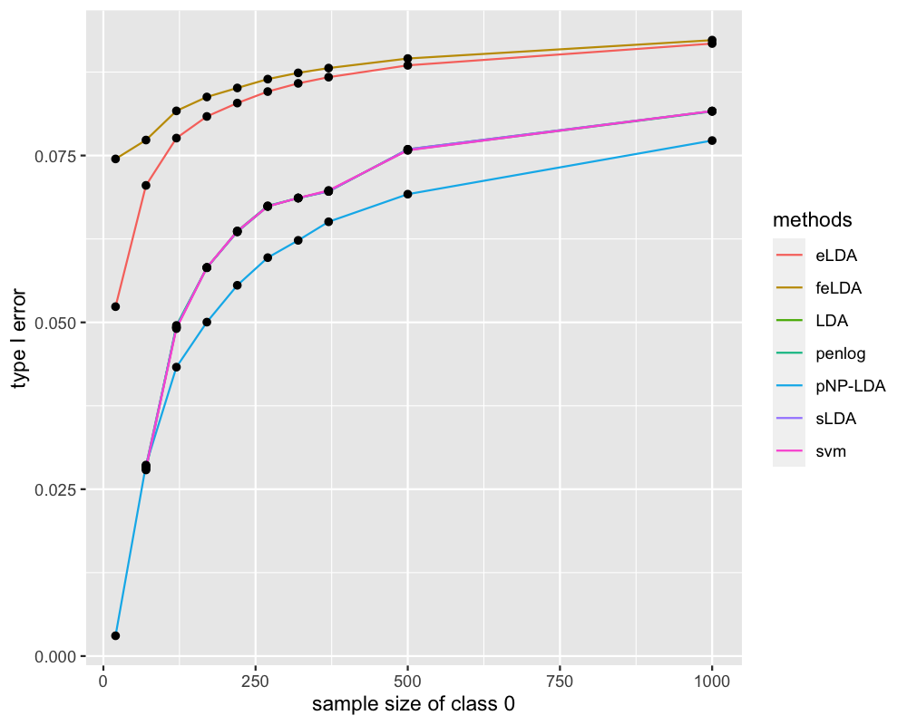
(a) Example 1a, type I error

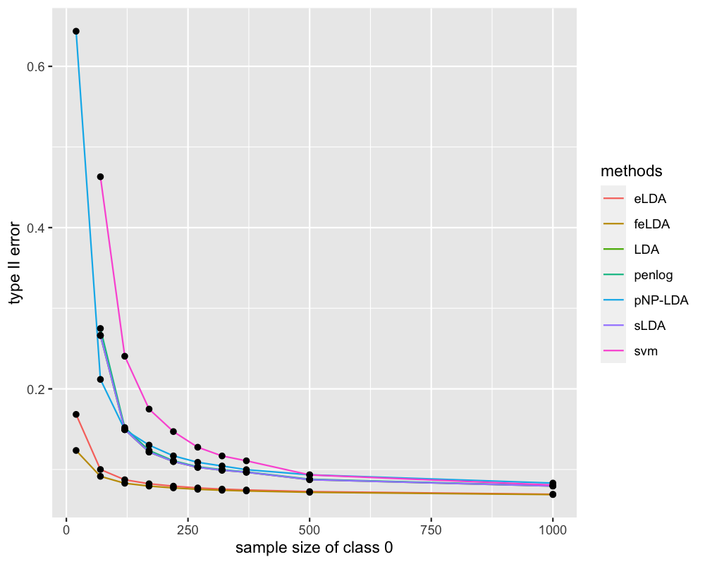
(b) Example 1a, type II error

The common setting shared by Examples 1c, 1c’ and 1c* includes balanced and fixed sample sizes, and increasing dimension $p$. Similarly, in the main text, we only present performance of Example 1c in Figure 2 and leave the comparison across Examples 1c, 1c’ and 1c* to Appendix Figure E.2. First, we observe from Figure 2 that both eLDA and feLDA dominate existing methods in terms of type II errors. Nevertheless, Example 1c shows that when $p$ gets to 20 and beyond, type I error of feLDA is no longer bounded by $\alpha=0.1$. Changing the violation rate $\delta$ from 0.1 to 0.05 and further to 0.01 hinders the growth of type I error of feLDA as $p$ increases, but does not solve the problem ultimately as illustrated in Figure E.2 panel (c) and (e). This is due to the construction of feLDA which is specifically designed for small $p$; when $p$ gets large, eLDA outperforms feLDA. Therefore, considering the performance across different $p$’s, eLDA performs the best among the seven methods. Second, as dimension $p$ increases, all of the type II errors slightly increase or remain stable as expected, except for that of pNP-LDA. This is due to a technical bound in the construction of the threshold of pNP-LDA, which becomes loose when $p$ is large.

Appendix Table E.2 presents the violation rates from Examples 1c, 1c’, and 1c*. Similar to what we have observed earlier, the five existing NP classifiers are relatively conservative and the observed violation rates of eLDA are mostly around the targeted $\delta$ in all the three sub-examples, while that of feLDA goes beyond the targeted $\delta$ as $p$ increases. When we decrease $\delta$ from 0.1 to 0.05 and further to 0.01, we have the following two observations: 1) the violation rates of the four NP umbrella algorithm based classifiers NP-LDA, NP-sLDA, NP-penlog and NP-svm stay the same in Examples 1c and 1c’. The violation rates decrease as we move to Example 1c*. This is due to the discrete combinatorial construction of the thresholds in umbrella algorithms and thus the observed violation rates present discrete changes in terms of $\delta$. In other words, not necessarily small changes in $\delta$ will lead to a change in the constructed classifier and the observed violation rates. For example, for NP umbrella algorithm based methods, the number of left-out class 0 observations is 63, and the threshold is constructed as the $k^{*}$-th order statistics of the classification scores of the left-out class 0 sample, where $k^{*}=\min\{k\in\{1,\cdots,63\}:\nu(k)<\delta\}$, and $\nu(k)=\sum_{j=k}^{63}{63\choose j}(1-\alpha)^{j}\alpha^{63-j}$. Plugging in $\alpha=0.1$, we could easily calculate that $k^{*}=61$ for both $\delta=0.1$ and $\delta=0.05$, since $\nu(61)=\sum_{j=61}^{63}{63\choose j}(1-0.1)^{j}0.1^{63-j}=0.042$ and $\nu(60)=0.113$. Furthermore, for $\delta=0.01$, the threshold changes as $k^{*}$ changes, since $0.042>0.01$; 2) pNP-LDA, eLDA, and feLDA have the parametric construction of the threshold and the observed violation rates of these methods respond to changes in $\delta$ more smoothly. Nevertheless, pNP-LDA is overly conservative, with the observed violation rate almost all 0.

Figure 2: Examples 1c, type I and type II errors for competing methods with increasing dimension $p$, $\delta=0.1$.

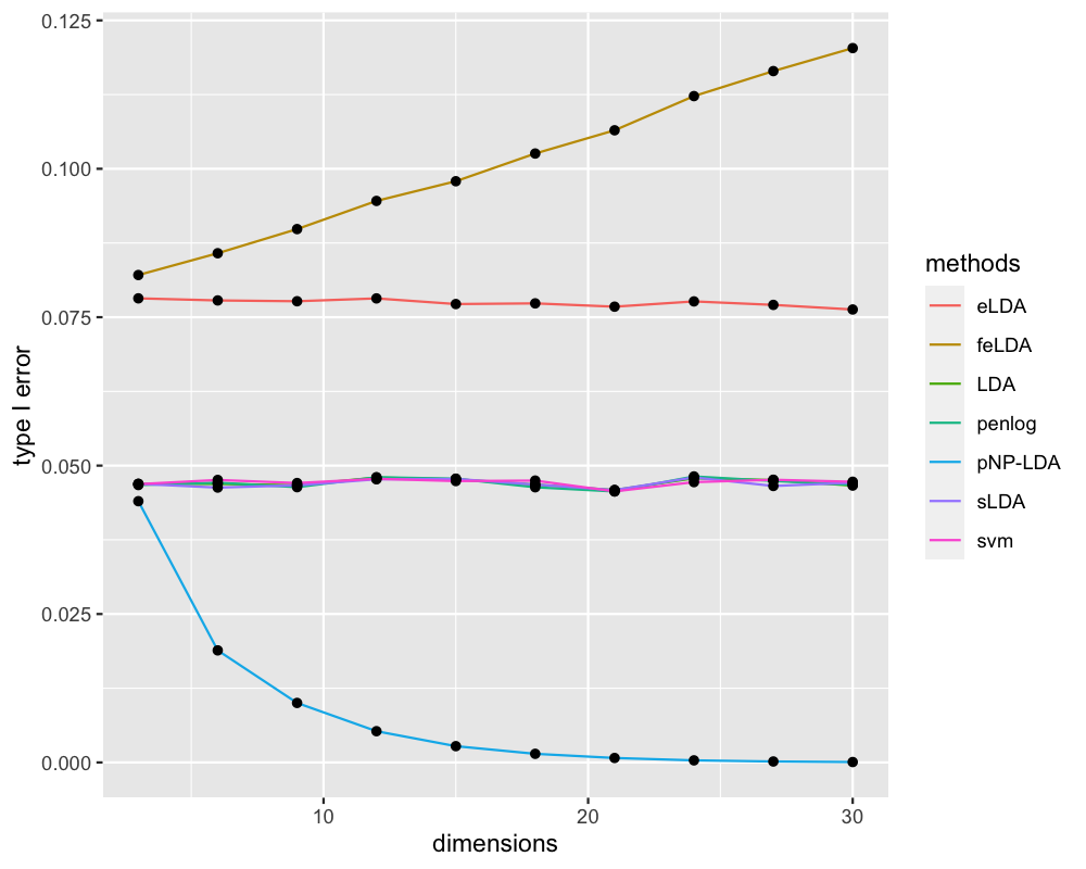
(a) Example 1c, type I error

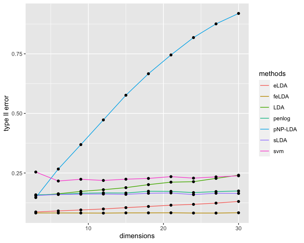
(b) Example 1c, type II error

Examples 1d and 1d’ also demonstrate the performances when dimension $p$ increases, but with unequal class sizes. We omit the details in the main due to similar messages, and refer interested readers to Appendix Figure E.3.

Example 2.

The data are generated from an LDA model with common covariance matrix $\Sigma$, where $\Sigma$ is set to be an AR(1) covariance matrix with $\Sigma_{ij}=0.5^{|i-j|}$ for all $i$ and $j$. $\bm{\beta}^{\text{Bayes}}=\Sigma^{-1}\bm{\mu}_{d}=C_{p}\cdot\bm{1}_{p}^{\top}$, $\bm{\mu}^{0}=\bm{0}_{p}$. Here, $C_{p}$ is a constant depending on $p$, such that the NP oracle classifier always has type II error $0.236$ for any choice of $p$ when $\alpha=0.1$. We set $\pi_{0}=\pi_{1}=0.5$ and $\alpha=\delta=0.1$.

1. $n_{0}=n_{1}=125$, varying $p\in\{3,6,9,12,15,18,21,24,27,30\}$

2. $n_{0}=125,n_{1}=500$, varying $p\in\{3,6,9,12,15,18,21,24,27,30\}$

Examples 2a and 2b are similar to Examples 1c and 1d, but their oracle projection direction $\bm{\beta}^{\text{Bayes}}$ is not sparse. Appendix Figure E.4 summarizes the results on type I and type II errors. The delivered messages are similar to those of Examples 1c and 1d: 1) while eLDA enjoys controlled type I errors under $\alpha=0.1$ for all $p$ in both Examples 2a and 2b, the type I errors of feLDA deteriorate above the target for large $p$; 2) eLDA and feLDA dominate all other competing methods in terms of type II errors. Observed violation rates from Examples 2a and 2b present similar messages as in Examples 1c and 1d, so we omit the table for those results.

We have also conducted experiments under non-Gaussian settings. In short, we observe that when sample size of class 0 is small, eLDA and feLDA clearly outperform all their competitors. As the sample size increases, the performances of most umbrella algorithm based classifiers begin to catch up and eventually outperform eLDA and feLDA. We believe this phenomenon is due to the fine calibration of the LDA model in the development of eLDA and feLDA, which leads to conservative results in heavy-tail distribution settings. Set-up of experiments and detail discussions are included in Appendix E.2.

6.2 Real Data Analysis

We analyze two real datasets. The first one is a lung cancer dataset (Gordon et al., 2002; Jin and Wang, 2016) that consists of gene expression measurements from 181 tissue samples. Among them, 31 are malignant pleural mesothelioma (MPM) samples and 150 are adenocarinoma (ADCA) samples. As MPM is known to be highly lethal pleural malignant and rare (in contrast to ADCA which is more common), misclassifying MPM as ADCA would incur more severe consequences. Therefore, we code MPM as class 0, and ADCA as class 1. The feature dimension of this dataset is $p=12{,}533$. First, we set $\alpha=0.01$ and $\delta=0.05$. Since the class 0 sample size is very small, none of the umbrella algorithm based NP classifiers are implementable. Hence, we only compare the performance of pNP-LDA with that of eLDA. We choose to omit feLDA here because we have found from the simulation studies that feLDA outperforms eLDA only when the dimension is extremely small (e.g., $p\leq 3$). On the other hand, since eLDA is designed for $p<n$ settings and pNP-LDA usually works poorly for large $p$, we first reduce the feature dimensionality to 40 by conducting two-sample t-test and selecting the 40 genes with smallest p-values. To provide a more complete story, we implemented further analysis with larger parameters ($\alpha=0.1$ and $\delta=0.4$) so that NP-sLDA, NP-penlog, NP-svm are also implementable. Those results are presented in Appendix Table E.4.

The experiment is repeated 100 times and the type I and type II errors are the averages over these 100 replications. In each replication, we randomly split the full dataset (class 0 and class 1 separately) into a training set (composed of 70% of the data), and a test set (composed of 30% of the data). We train the classifiers on the training set, with the feature selection step added before implementing eLDA and pNP-LDA. Then we apply the classifiers to the test set to compute the empirical type I and type II errors. Table 6.2 presents results from the parameter set $\alpha=0.01$ and $\delta=0.05$. We observe that while both eLDA and pNP-LDA achieve type I errors smaller than the targeted $\alpha=0.01$, pNP-LDA is overly conservative and has a type II error of 1. In contrast, eLDA provides a more reasonable type II error of 0.104, and the observed violation rate is 0.03 ($<0.05$).

Table 2: Lung cancer dataset

		pNP-LDA	eLDA
$\alpha=0.01$ $\delta=0.05$	type I error	.000	.003
	type II error	1	.104
	observed violation rate	0	.03

The second dataset was originally studied in Su et al. (2001). It contains microarray data from 11 different tumor cells, including 27 serous papillary ovarian adenocarcinomas, 8 bladder/ureter carcinomas, 26 infiltrating ductal breast adenocarcinomas, 23 colorectal adenocarcinomas, 12 gastroesophageal adenocarcinomas, 11 clear cell carcinomas of the kidney, 7 hepatocellular carcinomas, 26 prostate adenocarcinomas, 6 pancreatic adenocarcinomas, 14 lung adenocarcinomas carcinomas, and 14 lung squamous carcinomas. In more recent studies (Jin and Wang, 2016; Yousefi et al., 2010), the 11 different tumor cell types were aggregated into two classes, where class 0 contains bladder/ureter, breast, colorectal and prostate tumor cells, and class 1 contains the remaining groups. We follow Yousefi et al. (2010) in determining the binary class labels, and we work on the modified dataset with $n_{0}=83$, $n_{1}=91$ and $p=12{,}533$.

We repeat the data processing procedure as in the lung dataset, and report results from the parameter set $\alpha=0.01$ and $\delta=0.05$ in Table 6.2. While the sample size is too small for other umbrella algorithm based NP classifiers to work, the advantage of eLDA over pNP-LDA is obvious. The observed violation rate 0.15 is larger than the targeted $\delta=0.05$. However, we would like to emphasize that the observed violation rate in a real data study should not be interpreted as a close proxy to the true violation rate. First, the previous discussion on observed violation rate for simulation in the footnote also applies to the real data studies. Moreover, in simulations, samples are generated from population many times; however, in real data analysis, the one sample we have plays the role of population for repetitive sampling. Such substitute can be particularly inaccurate when the sample size is small.

Table 3: Cancer dataset in Su et al. (2001)

		pNP-LDA	eLDA
$\alpha=0.01$ $\delta=0.05$	type I error	.000	.008
	type II error	1	.437
	observed violation rate	0	.15

7 Discussion

Our current work initiates the investigations on non-splitting strategies under the NP paradigm. For future works, we can work in settings where $p$ is larger than $n$ by selecting features via various marginal screening methods (Fan and Song, 2010; Li et al., 2012) and/or may add structural assumptions to the LDA model. To accommodate diverse applications, one might also construct classifiers based on more complicated models, such as the quadratic discriminant analysis (QDA) model (Fan et al., 2015; Li and Shao, 2015; Yang and Cheng, 2018; Pan and Mai, 2020; Wang et al., 2021; Cai and Zhang, 2021).

Appendix A Further remark on Assumption 1

Previously, margin assumption and detection condition were assumed in Tong (2013) and subsequent works Zhao et al. (2016); Tong et al. (2020) for an NP classifier to achieve a diminishing excess type II error. Concretely, write the level-$\alpha$ NP oracle as ${\rm 1}\kern-2.40005pt{\rm I}(f_{1}({\bf x})/f_{0}({\bf x})>C^{*}_{\alpha})$, where $f_{1}$ and $f_{0}$ are class-conditional densities of the features, then the margin assumption assumes that

$${\rm I}\kern-1.79993pt{\rm P}(|f_{1}({\bf x})/f_{0}({\bf x})-C^{*}_{\alpha}|\leq\delta|Y=0)\leq C_{0}\delta^{\bar{\gamma}}\,,$$

for any $\delta>0$ and some positive constant $\bar{\gamma}$ and $C_{0}$. This is a low-noise condition around the oracle decision boundary that has roots in Polonik (1995); Mammen and Tsybakov (1999). On the other hand, the detection condition, which was coined in Tong (2013) and refined in Zhao et al. (2016), requires a lower bound:

$${\rm I}\kern-1.79993pt{\rm P}(C^{*}_{\alpha}\leq f_{1}({\bf x})/f_{0}({\bf x})\leq C^{*}_{\alpha}+\delta|Y=0)\geq C_{1}\delta^{\underset{\raise 2.10002pt\hbox{$\smash{\scriptscriptstyle-}$}}{\gamma}}\,,$$

for small $\delta$ and some positive constant $\underset{\raise 3.00003pt\hbox{$\smash{\scriptscriptstyle-}$}}{\gamma}$. In fact, $\delta^{\underset{\raise 2.10002pt\hbox{$\smash{\scriptscriptstyle-}$}}{\gamma}}$ can be generalized to $u(\delta)$, where $u(\cdot)$ is any increasing function on $R^{+}$ that might be $(f_{0},f_{1})$-dependent and $\lim_{\delta\to 0^{+}}u(\delta)=0$. The necessity of the detection condition under general models for achieving a diminishing excess type II error was also demonstrated in Zhao et al. (2016) by showing a counterexample that has fixed $f_{1}$ and $f_{0}$, i.e., when $p$ does not grow with $n$. Note that although the feature dimension $p$ considered in Zhao et al. (2016); Tong et al. (2020) can grow with $n$, both impose sparsity assumptions, and the “effective” dimensionality $s$ has the property that $s/n\to 0$. Hence previously, there were no theoretical results regarding the excess type II error when the effective feature dimensionality and the sample size are comparable.

Under Assumption 1, the marginal assumption and detection condition hold automatically. To see this, recall the level-$\alpha$ NP oracle classifier defined in (2.1), we can directly derive that for any $\delta>0$,

$$\quad{\rm I}\kern-1.79993pt{\rm P}(C^{*}_{\alpha}\leq f_{1}({\bf x})/f_{0}({\bf x})\leq C^{*}_{\alpha}+\delta|Y=0)$$

$$={\rm I}\kern-1.79993pt{\rm P}(F\leq(\Sigma^{-1}{\bm{\mu}}_{d})^{\top}{\bf x}\leq F+\delta|Y=0)$$

$$={\rm I}\kern-1.79993pt{\rm P}\big{(}F-{\bm{\mu}}_{d}^{\top}\Sigma^{-1}{\bm{\mu}}^{0}\leq(\Sigma^{-1}{\bm{\mu}}_{d})^{\top}({\bf x}-{\bm{\mu}}^{0})\leq F-{\bm{\mu}}_{d}^{\top}\Sigma^{-1}{\bm{\mu}}^{0}+\delta|Y=0\big{)}$$

$$={\rm I}\kern-1.79993pt{\rm P}\Big{(}\frac{F-{\bm{\mu}}_{d}^{\top}\Sigma^{-1}{\bm{\mu}}^{0}}{\sqrt{\varDelta_{d}}}\leq\mathcal{N}(0,1)\leq\frac{F-{\bm{\mu}}_{d}^{\top}\Sigma^{-1}{\bm{\mu}}^{0}+\delta}{\sqrt{\varDelta_{d}}}\Big{)}\,,$$

with the shorthand notation $F:=\sqrt{\varDelta_{d}}\,\Phi^{-1}(1-\alpha)+{\bm{\mu}}_{d}^{\top}\Sigma^{-1}{\bm{\mu}}^{0}$. The RHS above can be further simplified to get

$${\rm I}\kern-1.79993pt{\rm P}(F\leq(\Sigma^{-1}{\bm{\mu}}_{d})^{\top}{\bf x}\leq F+\delta|Y=0)=\Phi\Big{(}\Phi^{-1}(1-\alpha)+{\delta}/{\sqrt{\varDelta_{d}}}\,\Big{)}-(1-\alpha).$$

Thereby, using mean value theorem, we simply bound the above probability from above and below as

$${\rm I}\kern-1.79993pt{\rm P}(F\leq(\Sigma^{-1}{\bm{\mu}}_{d})^{\top}{\bf x}\leq F+\delta|Y=0) \leq\frac{1}{\sqrt{2\pi}}\exp{(-\frac{1}{2}\Phi_{\alpha}^{2})}\frac{\delta}{\sqrt{\varDelta_{d}}}\,,$$

$${\rm I}\kern-1.79993pt{\rm P}(F\leq(\Sigma^{-1}{\bm{\mu}}_{d})^{\top}{\bf x}\leq F+\delta|Y=0) \geq\frac{1}{\sqrt{2\pi}}\exp{\bigg{(}-\frac{1}{2}\Big{(}\Phi_{\alpha}+\frac{\delta}{\sqrt{\varDelta_{d}}}\Big{)}^{2}\bigg{)}}\frac{\delta}{\sqrt{\varDelta_{d}}}\,.$$

where we recall $\Phi_{\alpha}=\Phi^{-1}(1-\alpha)$. A similar upper bound can also be derived for ${\rm I}\kern-1.79993pt{\rm P}(F-\delta\leq(\Sigma^{-1}{\bm{\mu}}_{d})^{\top}{\bf x}\leq F|Y=0)$. These coincide with the aforementioned marginal assumption and detection condition.

Appendix B Proofs of Lemma 1 and Corollary 1

We first show the proof of Lemma 1 below.

Proof 2 (Proof of Lemma 1).

The statement (i) is easy to obtain by the definition of $\tilde{\phi}_{\alpha}^{*}(\cdot)$ in (3.1) and the definition of the type I error. Specifically,

$$R_{0}(\tilde{\phi}_{\alpha}^{*}) ={\rm I}\kern-1.79993pt{\rm P}\Big{(}\widehat{A}^{\top}({\bf x}-{\bm{\mu}}^{0})>\sqrt{\widehat{A}^{\top}\Sigma\widehat{A}}\,\Phi^{-1}(1-\alpha)\Big{|}{\bf x}\sim\mathcal{N}({\bm{\mu}}^{0},\Sigma)\Big{)}$$

$$=1-\Phi(\Phi^{-1}(1-\alpha))=\alpha\,.$$

Next, we establish statement (ii). By definition, we have

$$R_{1}(\tilde{\phi}_{\alpha}^{*}) ={\rm I}\kern-1.79993pt{\rm P}\Big{(}\widehat{A}^{\top}({\bf x}-{\bm{\mu}}^{1})\leq\sqrt{\widehat{A}^{\top}\Sigma\widehat{A}}\,\Phi^{-1}(1-\alpha)-\widehat{A}^{\top}{\bm{\mu}}_{d}\Big{|}{\bf x}\sim\mathcal{N}({\bm{\mu}}^{1},\Sigma)\Big{)}$$

$$=\Phi\Big{(}\Phi^{-1}(1-\alpha)-\frac{\widehat{A}^{\top}{\bm{\mu}}_{d}}{\sqrt{\widehat{A}^{\top}\Sigma\widehat{A}}}\,\Big{)}\,,$$

$$R_{1}({\phi}_{\alpha}^{*}) ={\rm I}\kern-1.79993pt{\rm P}\Big{(}(\Sigma^{-1}{\bm{\mu}}_{d})^{\top}{\bf x}<\sqrt{\varDelta_{d}}\,\Phi^{-1}(1-\alpha)+{\bm{\mu}}_{d}^{\top}\Sigma^{-1}{\bm{\mu}}^{0}\Big{|}{\bf x}\sim\mathcal{N}({\bm{\mu}}^{1},\Sigma)\Big{)}$$

$$=\Phi\Big{(}\Phi^{-1}(1-\alpha)-\sqrt{\varDelta_{d}}\,\Big{)}\,.$$ (B.1)

Lemma 1 and some elementary calculations lead to the conclusion: for any $\varepsilon\in(0,1/2)$ and $D>0$, when $n>n(\epsilon,D)$, with probability at least $1-n^{-D}$ we have,

$$\varDelta_{d}^{1/2}>\frac{\widehat{A}^{\top}{\bm{\mu}}_{d}}{\sqrt{\widehat{A}^{\top}\Sigma\widehat{A}}}=\varDelta_{d}^{1/2}+O\big{(}r\varDelta_{d}^{1/2}\big{)}+O\big{(}n^{-\frac{1}{2}+\varepsilon}(1+\varDelta_{d}^{1/2})\big{)}\,.$$

Moreover, it is straightforward to check

$$\exp\Big{(}-\frac{1}{2}{\Big{(}\Phi^{-1}(1-\alpha)-\varDelta_{d}^{1/2}\,\Big{)}^{2}}\Big{)}\asymp\exp\Big{(}-\frac{c\varDelta_{d}}{2}\Big{)}\,.$$

Thus, we conclude that there exists some fixed constant C which may depend on $c_{0},c_{1},c_{2}$ and $\alpha$ such that for any $\varepsilon\in(0,1/2)$ and $D>0$, when $n\geq n(\varepsilon,D)$, with probability at least $1-n^{-D}$, we have

$$R_{1}(\tilde{\phi}_{\alpha}^{*})-R_{1}({\phi}_{\alpha}^{*})\leq C\big{(}r+n^{-\frac{1}{2}+\varepsilon}\big{)}\varDelta_{d}^{1/2}\exp\Big{(}-\frac{c\varDelta_{d}}{2}\Big{)}\,.$$

This finished our proof.

At the end of this section, we sketch the proof of Corollary 1.

Proof 3 (Proof of Corollary 1).

By the definition of $\widetilde{F}(\widehat{\Sigma},\hat{\bm{\mu}}^{0})$ and $\widetilde{C}_{\alpha}^{p}$ in (3.7), (3.8), under the setting of $p=O(1)$, we observe that

$$\widetilde{F}(\widehat{\Sigma},\hat{\bm{\mu}}^{0})=\widehat{F}(\widehat{\Sigma},\hat{\bm{\mu}}^{0})+O_{\prec}\big{(}n^{-1}\varDelta_{d}^{\frac{1}{2}}\big{)}\,,$$

$$\widetilde{C}_{\alpha}^{p}=\widehat{C}_{\alpha}^{p}+O_{\prec}\big{(}n^{-1}\varDelta_{d}^{\frac{1}{2}}\big{)}\,.$$

Then, similarly to the proof of Theorem 1, with the aid of Remark 3 and Remark 4, we conclude the results in the same manner; hence we omit the details.

Appendix C Proofs for Section 4

C.1 Proof of Lemma 1

Part (i) is obvious from Definition 1. For any fixed $\varrho>0$, we have

$$|{\rm I}\kern-1.79993pt{\rm E}\mathsf{X}_{1}| \leq{\rm I}\kern-1.79993pt{\rm E}|\mathsf{X}_{1}{\rm 1}\kern-2.40005pt{\rm I}(|\mathsf{X}_{1}|\leq N^{\varrho}\Phi)|+{\rm I}\kern-1.79993pt{\rm E}|\mathsf{X}_{1}{\rm 1}\kern-2.40005pt{\rm I}(|\mathsf{X}_{1}|\geq N^{\varrho}\Phi)|$$

$$\leq N^{\varrho}\Phi+N^{C}{\rm I}\kern-1.79993pt{\rm P}(|\mathsf{X}_{1}|\geq N^{\varrho}\Phi)=O(N^{\varrho}\Phi)$$

for for sufficiently large $N\geq N_{0}(\varrho)$. This proves part (ii).

C.2 Proof of Proposition 1

Define

$$\mathcal{D}\equiv\mathcal{D}(\tau):=\{z\in\mathbb{C}^{+}:-\frac{\lambda_{-}}{2}<\Re{z}<\frac{\lambda_{-}}{2},0<\Im{z}\leq\tau^{-1}\}\,.$$ (C.1)

All the estimates in Proposition 1 can be separately shown for the case of $p>n^{\epsilon}$ for some fixed small $\epsilon>0$ and the case of $p<n^{\epsilon}$. We first show all the estimates hold for the case $l=0$ and then proceed to the case of $l\geq 1$.

$\bullet$ For the case of $l=0$.

In the regime that $p\geq n^{\epsilon}$ for some fixed small $\epsilon>0$, (4.5) can be derived from the entrywise local Marchenko-Pastur law for extended spectral domain in Theorem 4.1 of Bloemendal et al. (2014). We emphasize that originally in Bloemendal et al. (2014) the results are not provided for extended spectral domain one only need to adapt the arguments in Proposition 3.8 of Bloemendal et al. (2016) to extend the results.

The estimates of (4.7) can be obtained by the rigidity estimates of eigenvalues in (Bloemendal et al., 2014, Theorem 2.10). We remark that we get the improved version in the second estimate of (4.8) due to the trivial bound $z=O(1)$, for $z\in\mathcal{D}^{0}$, while for $z\in\mathcal{D}$, we crudely bound $|z|$ by $r^{-\frac{1}{2}}$. For (4.6), by noticing that ${X}^{\top}\mathcal{G}_{1}=\mathcal{G}_{2}{X}$, one only needs to show the first estimate of (4.6). Using singular value decomposition (SVD) of ${X}$, i,e., ${X}=U^{\top}(\Lambda^{\frac{1}{2}},0)V$, where the diagonal matrix $\Lambda^{\frac{1}{2}}$ collects the singular values of $X$ in a descending order, we arrive at

$$\big{(}{X}^{\top}\mathcal{G}_{1}(z)\big{)}_{i^{\prime}i}=V_{i^{\prime}}^{\top}\left(\begin{array}[]{c}\Lambda^{\frac{1}{2}}(\Lambda-z)^{-1}\\ {\bf 0}\end{array}\right)U_{i},\qquad\Lambda:=\text{diag}(\lambda_{1},\ldots,\lambda_{p})$$

and $U_{i}$, $V_{i^{\prime}}$ are independent and uniformly distributed on $\mathbf{S}^{p-1}$ and $\mathbf{S}^{n-1}$, respectively, thanks to the fact that ${X}$ is a GOE matrix. Here we abbreviate $\lambda_{i}(H)$ by $\lambda_{i}$. Then we can further write

$$\big{(}{X}^{\top}\mathcal{G}_{1}(z)\big{)}_{i^{\prime}i} \overset{\rm d}{=}\sum_{i=1}^{p}g_{i}\tilde{g}_{i}\frac{\sqrt{\lambda}_{i}}{\lambda_{i}-z}\frac{1}{\|{\bf g}\|\|{\bf\tilde{g}}\|}$$

$$=\sum_{i=1}^{p}g_{i}\tilde{g}_{i}\frac{\sqrt{\lambda}_{i}}{\lambda_{i}-z}\Big{(}1-\frac{\|{\bf g}\|^{2}-1}{2}+O_{\prec}(n^{-1})\Big{)}\Big{(}1-\frac{\|{\bf\tilde{g}}\|^{2}-1}{2}+O_{\prec}(p^{-1})\Big{)},$$ (C.2)

where ${\bf g}:=(g_{1},\cdots,g_{p})\sim\mathcal{N}(0,\frac{1}{p}I_{p})$, ${\bf\tilde{g}}:=(\tilde{g}_{1},\cdots,\tilde{g}_{n})\sim\mathcal{N}(0,\frac{1}{n}I_{n})$ and they are independent. The leading term on the RHS of (C.2) is $\sum_{i=1}^{p}g_{i}\tilde{g}_{i}\frac{\sqrt{\lambda}_{i}}{\lambda_{i}-z}$. By the rigidity of eigenvalues, we easily get that $\sqrt{\lambda}_{i}/(\lambda_{i}-z)\asymp r^{\frac{1}{4}}$ uniformly for $z\in\mathcal{D}$ with high probability. Further applying the randomness of $g_{i}$’s and $\tilde{g}_{i}$’s, it is easy to conclude the first estimate in (4.6). The second estimate with the extension in (4.8) holds naturally from ${X}^{\top}\mathcal{G}_{1}=\mathcal{G}_{2}{X}$ and the facts that $|z|\leq r^{-\frac{1}{2}}$ for $z\in\mathcal{D}$, $|z|=O(1)$ for $z\in\mathcal{D}^{0}$.

In the regime that $p<n^{\epsilon}$ for sufficiently small $\epsilon$. We first write

$${X}{X}^{\top}=r^{-\frac{1}{2}}I_{p}+{G},$$

where ${G}$ is a $p$ by $p$ matrix defined entrywise by ${G}_{ij}={\bf x}_{i}^{\top}{\bf x}_{j}-\mathbb{E}{\bf x}_{i}^{\top}{\bf x}_{j}$ and ${\bf x}_{i}$ represents the i-th row of ${X}$. One can easily see that ${G}_{ij}$ is asymptotically centred Gaussian with variance $1/p$ by CLT. Thus we can crudely estimate ${G}_{ij}=O_{\prec}(p^{-1/2})$ and $\|{G}\|\leq\|G\|_{\text{HS}}=O_{\prec}(\sqrt{p}\,)$. Then, for $\mathcal{G}_{1}$, we can obtain that for $z\in\mathcal{D}$,

$$\mathcal{G}_{1}=(r^{-\frac{1}{2}}-z)^{-1}\Big{(}I_{p}+(r^{-\frac{1}{2}}-z)^{-1}{G}\Big{)}^{-1}=(r^{-\frac{1}{2}}-z)^{-1}I_{p}-(r^{-\frac{1}{2}}-z)^{-2}G+O_{\prec}\big{(}r^{\frac{3}{2}}p\big{)}$$

here with a little abuse of notation, we used $O_{\prec}\big{(}r^{\frac{3}{2}}p\big{)}$ to represent the higher order term of matrix form whose operator norm is $O_{\prec}\big{(}r^{\frac{3}{2}}p\big{)}$. Choosing $\epsilon$ sufficiently small so that $p^{3}n^{-\frac{1}{2}}=o(1)$. After elementary calculation, we further have that

$$(\mathcal{G}_{1})_{ij}=(r^{-\frac{1}{2}}-z)^{-1}\delta_{ij}-(r^{-\frac{1}{2}}-z)^{-2}{G}_{ij}+O_{\prec}(n^{-1})=(r^{-\frac{1}{2}}-z)^{-1}\delta_{ij}+O_{\prec}(n^{-\frac{1}{2}}r^{\frac{1}{2}}),$$

$$m_{1}(z)-(r^{-\frac{1}{2}}-z)^{-1}=O_{\prec}(r^{\frac{3}{2}}),$$ (C.3)

which by the fact that $r^{\frac{3}{2}}\ll n^{-\frac{1}{2}}r^{\frac{1}{2}}$ indeed imply the first estimate in (4.5) for the case $l=0$. By using the identity $z\mathcal{G}_{2}(z)={X}^{\top}\mathcal{G}_{1}(z){X}-I_{p}$, we also have that

$$(z\mathcal{G}_{2}(z))_{i^{\prime}j^{\prime}}=-\delta_{i^{\prime}j^{\prime}}+(r^{-\frac{1}{2}}-z)^{-1}({X}^{\top}{X})_{i^{\prime}j^{\prime}}-(r^{-\frac{1}{2}}-z)^{-2}({X}^{\top}{G}{X})_{i^{\prime}j^{\prime}}+O_{\prec}(n^{-1}),$$

$$zm_{2}(z)=-1+r(1+zm_{1}(z))=-1+r^{\frac{1}{2}}(r^{-\frac{1}{2}}-z)^{-1}+O_{\prec}(r^{\frac{3}{2}}).$$ (C.4)

It is easy to see that $({X}^{\top}{X})_{i^{\prime}j^{\prime}}=({\bf x}^{i^{\prime}})^{\top}{\bf x}^{j^{\prime}}=r^{\frac{1}{2}}\delta_{i^{\prime}j^{\prime}}+O_{\prec}(n^{-1/2})$, where ${\bf x}^{i^{\prime}}$ is the $i^{\prime}$-th column of ${X}$. Furthermore, $|({X}^{\top}G{X})_{i^{\prime}j^{\prime}}|=|({\bf x}^{i^{\prime}})^{\top}G{\bf x}^{j^{\prime}}|\leq\|G\|\|{\bf x}^{i^{\prime}}\|\|{\bf x}^{j^{\prime}}\|=O_{\prec}(n^{-1/2}p)$. We then see that

$$(z\mathcal{G}_{2}(z))_{i^{\prime}j^{\prime}}-zm_{2}(z)\delta_{i^{\prime}j^{\prime}}=O_{\prec}(n^{-\frac{1}{2}}r^{\frac{1}{2}}).$$

Thus, we can conclude the second estimate in (4.5). Next, for the two estimates in (4.6), we only need to focus on the former one in light of ${X}^{\top}\mathcal{G}_{1}=\mathcal{G}_{2}{X}$ and the facts $|z|\leq r^{-\frac{1}{2}}$ for $z\in\mathcal{D}$, $|z|=O(1)$ for $z\in\mathcal{D}^{0}$. Similarly to the above discussion, we have

$$({X}^{\top}\mathcal{G}_{1}(z))_{i^{\prime}i}=(r^{-\frac{1}{2}}-z)^{-1}X_{ii^{\prime}}-(r^{-\frac{1}{2}}-z)^{-2}({X}^{\top}G)_{i^{\prime}i}+O_{\prec}(n^{-1}p^{2}r^{\frac{1}{4}})=O_{\prec}(n^{-\frac{1}{2}}r^{\frac{1}{4}})$$ (C.5)

following from the facts that $X_{ii^{\prime}}=O_{\prec}(n^{-\frac{1}{2}}r^{-\frac{1}{4}})$, $|({X}^{\top}G)_{i^{\prime}i}|\leq\|G\||({X}^{\top}{X})_{i^{\prime}i^{\prime}}|^{1/2}=O_{\prec}(r^{1/4}\sqrt{p})$, and $p^{2}n^{-\frac{1}{2}}=o(1)$. This proved (4.6). We then turn to the estimates in (4.7). Note that $G_{ii}$ are i.i.d. random variables of order $O_{\prec}\big{(}p^{-\frac{1}{2}}\big{)}$, for $1\leq i\leq p$. Hence by CLT, $p^{-1}\sum_{i=1}^{p}G_{ii}$ is crudely of order $O_{\prec}(p^{-1})$. Applying the first estimate in (C.3), we have

$$m_{1n}(z) =\frac{1}{p}\sum_{i=1}^{p}(\mathcal{G}_{1})_{ii}=(r^{-\frac{1}{2}}-z)^{-1}+(r^{-\frac{1}{2}}-z)^{-2}\frac{1}{p}\sum_{i=1}^{p}G_{ii}+O_{\prec}(n^{-1})$$

$$=(r^{-\frac{1}{2}}-z)^{-1}+O_{\prec}(n^{-1}).$$

The above estimate, together with the second equation in (C.3) and the estimate $r^{\frac{3}{2}}\ll n^{-1}$, yields the first estimate in (4.7). The second estimate in (4.7) can be concluded simply by using the identity $zm_{2n}(z)=-1+r(1+zm_{1n}(z))$ and $zm_{2}(z)=-1+r(1+zm_{1}(z))$, since

$$|rzm_{1n}(z)-rzm_{1}(z)|\prec r|z||m_{1n}(z)-m_{1}(z)|\prec n^{-1}r^{\frac{1}{2}}$$

uniformly for $z\in\mathcal{D}$. Particularly for $z\in\mathcal{D}^{0}$, since $|z|=O(1)$, the bound above can be further improved to $n^{-1}r$.

Therefore, we proved the estimates (4.5)-(4.7) uniformly for $z\in\mathcal{D}$ in the case of $l=0$. Since $\mathcal{D}^{0}$ is simply a subset of $\mathcal{D}$, we trivially have the results uniformly for $z\in\mathcal{D}^{0}$. Now, we will proceed to the case that $l\geq 1$ by using the estimates for $z\in\mathcal{D}$.

$\bullet$ For the case of $l\geq 1$.

We can derive the estimates easily from the case $l=0$ by using Cauchy integral with the radius of the contour taking value $|z-\lambda_{-}|/4\asymp r^{-\frac{1}{2}}$. Note that for any $z\in\mathcal{D}^{0}$, the contour $\Gamma$ centred at $z$ with radius $|z-\lambda_{-}|/4$ still lies in the regime $\mathcal{D}$, hence all the estimates (4.5)-(4.7) hold uniformly on the contour. Moreover, we shall see that

$$\Big{|}\big{(}\mathcal{G}_{1}^{(l)}(z)\big{)}_{ij}-m_{1}^{(l)}(z)\delta_{ij}\bigg{|}\asymp\Big{|}\oint_{\Gamma}\frac{\big{(}\mathcal{G}_{1}(\tilde{z})\big{)}_{ij}-m_{1}(\tilde{z})\delta_{ij}}{(\tilde{z}-z)^{l+1}}{\rm d}\tilde{z}\bigg{|}\prec\frac{n^{-\frac{1}{2}}r^{\frac{1}{2}}}{|z-\lambda_{-}|^{l}}=n^{-\frac{1}{2}}r^{\frac{1+l}{2}}.$$

Similarly, we can show the error bounds for the other terms stated in (4.5)-(4.7).

Appendix D Proofs of Lemma 1 and Proposition 1

In this section, we prove Lemma 1 and Proposition 1, which are the key technical ingredients of the proofs of our main theorem. We separate the discussion into three subsections: in the first subsection we will show the proof of Lemma 1; then followed by the proof of Proposition 1 in the second subsection; in the last subsection, we provide the proofs for some technical results in the first two subsections. In advance of the proofs, we discuss some identities regarding Stieltjes transforms $m_{1}(z),m_{2}(z)$ (see (4.2) for definitions) and list some basic identities of Green functions which will be used frequently throughout this section.

Using (4.2) and (4.3), one can easily derive the following identities

$$m_{1}=-\frac{1}{z(1+r^{-1/2}m_{2})}\,,\quad 1+zm_{1}=\frac{1+zm_{2}}{r}\,,\quad r^{-1/2}(zm_{2})^{\prime}+1=\frac{m_{1}^{\prime}}{m_{1}^{2}}\,.$$ (D.1)

We remark that since our discussion is based on the assumption $r\equiv r_{n}\to r_{0}\in[0,1)$, then by definition, $\lambda_{-}=r^{1/2}+r^{-1/2}-2=O(r^{-1/2})$. This implies the support of $\nu_{\text{MP},a}({\rm d}x)$ for $a=1,2$ stays away from $0$ by $O(r^{-1/2})$ distance. For the special case $z=0$, $m_{1}(z)$ is well-defined and analytic at $z=0$ since $r<1$. More specifically, $m_{1}(0)=\sqrt{r}/(1-r)$ by the first equation of (4.3). In contrast, $z=0$ is a pole of $m_{2}(z)$ due to the $(1-r)$ point mass at $0$ (see MP law $\nu_{\text{MP},2}({\rm d}x)$ in (4.1)). However, the singularity at $z=0$ is removable for $zm_{2}(z)$. We can get $zm_{2}(z)|_{z=0}=r-1$ by simple calculations of the second equation of (4.2).We write $\widehat{m}_{2}(z):=zm_{2}(z)$ for simplicity. Let us simply list several results of functions in terms of $m_{1,2}$ at $z=0$ which can checked easily from either (4.2) or (D.1).

$$m_{1}(0)=\frac{\sqrt{r}}{1-r}\,,\quad m_{1}^{\prime}(0)=\frac{r}{(1-r)^{3}}\,;$$ (D.2)

$$\widehat{m}_{2}(0)=r-1\,,\quad\widehat{m}_{2}^{\prime}(0)=\frac{r^{3/2}}{1-r}\,.$$ (D.3)

Next for the Green functions $\mathcal{G}_{1}$, $\mathcal{G}_{2}$, we have some basic and useful identities which can be easily checked by some elementary computations.

$$\mathcal{G}_{1}^{l}=\frac{1}{(l-1)!}\frac{\partial^{l-1}\mathcal{G}_{1}}{\partial z^{l-1}}=\frac{1}{(l-1)!}\mathcal{G}_{1}^{(l-1)}\,,$$ (D.4)

$$\mathcal{G}_{1}^{l}{X}{X}^{\top}=\mathcal{G}_{1}^{l-1}+z\mathcal{G}_{1}^{l},\quad{X}^{\top}\mathcal{G}_{1}^{l}{X}=\mathcal{G}_{2}^{l}{X}^{\top}{X}=\mathcal{G}_{2}^{l-1}+z\mathcal{G}_{2}^{l}\,.$$ (D.5)

D.1 Proof of Lemma 1

We start with the proof of (5.2). Applying Woodbury matrix identity, from (2.4), we see that

$$\widehat{\Sigma}^{-1} =\frac{n-2}{n\sqrt{r}}\Sigma^{-\frac{1}{2}}\Big{(}\mathcal{G}_{1}(0)+\mathcal{G}_{1}(0)X{E}\mathcal{I}_{2}^{-1}{E}^{\top}{X}^{\top}\mathcal{G}_{1}(0)\Big{)}\Sigma^{-\frac{1}{2}}\,,$$ (D.6)

where we introduced the notation

$$\mathcal{I}_{2}:=I_{2}-{E}^{\top}{X}^{\top}\mathcal{G}_{1}(0)X{E}\,.$$

Recall the definition ${E}=({\bf e}_{0},{\bf e}_{1})$. By the second identity in (D.5) and the second estimate of (4.9), we have the estimate

$${\bf u}^{\top}{X}^{\top}\mathcal{G}_{1}^{a}(z){X}{\bf v}=(1+zm_{2}(z))^{(a-1)}{\bf u}^{\top}{\bf v}+O_{\prec}(n^{-\frac{1}{2}}r^{\frac{a}{2}})$$ (D.7)

for arbitrary unit vectors ${\bf u},{\bf v}$ and any integer $a\geq 1$. Further by $\widehat{m}_{2}(0)=zm_{2}(z)\Big{|}_{z=0}=r-1$, we obtain

$${\bf e}_{0}^{\top}{{X}}^{\top}\mathcal{G}_{1}(0){X}{\bf e}_{1}=O_{\prec}(n^{-1/2}r^{1/2}),\quad 1-{\bf e}_{i}^{\top}{{X}}^{\top}\mathcal{G}_{1}(0){X}{\bf e}_{i}=1-r+O_{\prec}(n^{-1/2}r^{1/2})\,,\;i=1,2\,.$$

Then,

$$\mathcal{I}_{2}^{-1}=\frac{1}{1-r}\,I_{2}+\Delta\,,$$ (D.8)

where $\Delta$ represents a $2\times 2$ matrix with $\|\Delta\|=O_{\prec}(n^{-1/2}r^{1/2})$. Plugging (D.8) into (D.6), we can write

$$\widehat{\Sigma}^{-1}=\frac{n-2}{n\sqrt{r}}\Sigma^{-\frac{1}{2}}\mathcal{G}_{1}(0)\Sigma^{-\frac{1}{2}}+\frac{n-2}{n(1-r)\sqrt{r}}\sum_{i=1,2}\Sigma^{-\frac{1}{2}}\mathcal{G}_{1}(0){X}{\bf e}_{i}{\bf e}_{i}^{\top}{X}^{\top}\mathcal{G}_{1}(0)\Sigma^{-\frac{1}{2}}+\widehat{\Delta}\,,$$ (D.9)

where ^Δ=n-2nr Σ^-12G_1(0)XEΔE^⊤X^⊤G_1(0)Σ^-12 , and it is easy to check $\|\widehat{\Delta}\|\prec n^{-1/2}r^{1/2}$.

With the above preparation, we now compute the leading term of $\widehat{A}^{\top}\widehat{\Sigma}\widehat{A}$. Recall $\widehat{A}=\widehat{\Sigma}^{-1}\hat{\bm{\mu}}_{d}$. We have

$$\widehat{A}^{\top}\widehat{\Sigma}\widehat{A}=\hat{\bm{\mu}}_{d}^{\top}\widehat{\Sigma}^{-1}\hat{\bm{\mu}}_{d} =\sqrt{r}{\bf v}_{1}^{\top}{X}^{\top}\Sigma^{\frac{1}{2}}\widehat{\Sigma}^{-1}\Sigma^{\frac{1}{2}}{X}{\bf v}_{1}+{\bm{\mu}}_{d}^{\top}\widehat{\Sigma}^{-1}{\bm{\mu}}_{d}+2r^{\frac{1}{4}}{\bf v}_{1}^{\top}{X}^{\top}\Sigma^{\frac{1}{2}}\widehat{\Sigma}^{-1}{\bm{\mu}}_{d}$$

$$=:T_{1}+T_{2}+T_{3}\,.$$ (D.10)

For $T_{1}$, with (D.9), we have

$$T_{1} =\frac{n-2}{n}\,{\bf v}_{1}^{\top}{X}^{\top}\mathcal{G}_{1}(0){X}{\bf v}_{1}+\frac{n-2}{n(1-r)}\,{\bf v}_{1}^{\top}{X}^{\top}\mathcal{G}_{1}(0){X}\Big{(}\sum_{i=0,1}{\bf e}_{i}{\bf e}_{i}^{\top}\Big{)}{X}^{\top}\mathcal{G}_{1}(0){X}{\bf v}_{1}$$

$$\qquad+\sqrt{r}{\bf v}_{1}^{\top}{X}^{\top}\Sigma^{\frac{1}{2}}\widehat{\Delta}\Sigma^{\frac{1}{2}}{X}{\bf v}_{1}$$

$$=r\|{\bf v}_{1}\|^{2}+\frac{r^{2}}{1-r}\Big{(}\big{(}{\bf v}_{1}^{\top}{\bf e}_{0}\big{)}^{2}+\big{(}{\bf v}_{1}^{\top}{\bf e}_{1}\big{)}^{2}\Big{)}+O_{\prec}(n^{-\frac{1}{2}}r^{\frac{1}{2}})\,.$$ (D.11)

Here in the last step, we repeatedly used the estimate (D.7) and $1+zm_{2}(z)|_{z=0}=r$. In addition, for the last term of the second line of (D.1), we trivially bound it by

$$\sqrt{r}{\bf v}_{1}^{\top}{X}^{\top}\Sigma^{\frac{1}{2}}\widehat{\Delta}\Sigma^{\frac{1}{2}}{X}{\bf v}_{1}\leq\|\widehat{\Delta}\|\|\Sigma\|(\sqrt{r}{\bf v}_{1}^{\top}{X}^{\top}{X}{\bf v}_{1})=O_{\prec}(n^{-\frac{1}{2}}r^{\frac{1}{2}})\,.$$

Similarly, for $T_{2}$, we have

$$T_{2} =\frac{n-2}{n\sqrt{r}}\,{\bf u}_{1}^{\top}\ \mathcal{G}_{1}(0){\bf u}_{1}+\frac{n-2}{n(1-r)\sqrt{r}}\,{\bf{u}}_{1}^{\top}\mathcal{G}_{1}(0){X}\Big{(}\sum_{i=0,1}{\bf e}_{i}{\bf e}_{i}^{\top}\Big{)}{X}^{\top}\mathcal{G}_{1}(0){\bf u}_{1}+{\bf u}_{1}^{\top}\Sigma^{\frac{1}{2}}\widehat{\Delta}\Sigma^{\frac{1}{2}}{\bf u}_{1}$$

$$=\frac{\|{\bf u}_{1}\|^{2}}{1-r}+O_{\prec}(n^{-\frac{1}{2}}\|{\bf u}_{1}\|^{2})\,,$$ (D.12)

where we employed the shorthand notation

$${\bf u}_{1}:=\Sigma^{-\frac{1}{2}}{\bm{\mu}}_{d}\,.$$ (D.13)

Here in (D.12), we applied the estimates

$${\bf u}_{1}^{\top}\ \mathcal{G}_{1}(0){\bf u}_{1}=m_{1}(0)\|{\bf u}_{1}\|^{2}+O_{\prec}(n^{-\frac{1}{2}}r^{\frac{1}{2}}\|{\bf u}_{1}\|^{2})$$ (D.14)

$${\bf u}_{1}^{\top}\mathcal{G}_{1}(z){X}{\bf e}_{i}=O_{\prec}(n^{-\frac{1}{2}}r^{\frac{1}{4}}\|{\bf u}_{1}\|)=O_{\prec}\big{(}n^{-\frac{1}{2}}r^{\frac{1}{4}}\|{\bf u}_{1}\|\big{)},\quad i=0,1\,.$$ (D.15)

with the fact $m_{1}(0)=1/(1-r)$. Next, we turn to estimate $T_{3}$. Similarly, we have

$$T_{3} =\frac{2(n-2)}{nr^{\frac{1}{4}}}{\bf v}_{1}^{\top}{X}^{\top}\mathcal{G}_{1}(0){\bf u}_{1}+\frac{2(n-2)}{n(1-r)r^{\frac{1}{4}}}{\bf v}_{1}^{\top}{X}^{\top}\mathcal{G}_{1}(0){X}\Big{(}\sum_{i=0,1}{\bf e}_{i}{\bf e}_{i}^{\top}\Big{)}{X}^{\top}\mathcal{G}_{1}(0){\bf u}_{1}+O_{\prec}(n^{-\frac{1}{2}}r^{\frac{1}{2}}\|{\bf u}_{1}\|)$$

$$=O_{\prec}(n^{-\frac{1}{2}}\|{\bf u}_{1}\|)\,.$$

Therefore, we arrive at

$$\widehat{A}^{\top}\widehat{\Sigma}\widehat{A} =\frac{r}{1-r}\|{\bf v}_{1}\|^{2}+\frac{1}{1-r}\|{\bf u}_{1}\|^{2}+O_{\prec}\big{(}n^{-\frac{1}{2}}(r^{\frac{1}{2}}+\|{\bf u}_{1}\|^{2}+\|{\bf u}_{1}\|)\big{)}\,.$$

This proved (5.2).

To proceed, we estimate $\widehat{A}^{\top}\Sigma\widehat{A}$. By definition,

$$\widehat{A}^{\top}\Sigma\widehat{A}=\Big{(}\frac{n-2}{n\sqrt{r}}\Big{)}^{2}\hat{\bm{\mu}}_{d}^{\top}\Sigma^{-\frac{1}{2}}H_{E}^{-2}\Sigma^{-\frac{1}{2}}\hat{\bm{\mu}}_{d}\,,$$

where we introduced the notation

$$H_{E}:={{X}}(I_{n}-{{E}}{{E}}^{\top}){{X}}^{\top}.$$

Applying Woodbury matrix identity again, we have

$$H_{E}^{-2} =\mathcal{G}_{1}^{2}(0)+\mathcal{G}_{1}^{2}(0){X}{E}\mathcal{I}_{2}^{-1}{E}^{\top}{{X}}^{\top}\mathcal{G}_{1}(0)$$

$$\quad+\mathcal{G}_{1}(0){X}{E}\mathcal{I}_{2}^{-1}{E}^{\top}{{X}}^{\top}\mathcal{G}_{1}^{2}(0)+\Big{(}\mathcal{G}_{1}(0){X}{E}\mathcal{I}_{2}^{-1}{E}^{\top}{{X}}^{\top}\mathcal{G}_{1}(0)\Big{)}^{2}.$$ (D.16)

Analogously to the way we deal with $\widehat{A}^{\top}\widehat{\Sigma}\widehat{A}$, applying the representation of $\hat{\bm{\mu}}_{d}$ in (2.6) and also the notation in (D.13), we can write

$$\widehat{A}^{\top}\Sigma\widehat{A} =\Big{(}\frac{n-2}{n}\Big{)}^{2}r^{-\frac{1}{2}}{\bf v}_{1}^{\top}{X}^{\top}H_{E}^{-2}{X}{\bf v}_{1}+\Big{(}\frac{n-2}{n}\Big{)}^{2}r^{-1}{\bf u}_{1}^{\top}H_{E}^{-2}{\bf u}_{1}$$

$$\qquad+2\Big{(}\frac{n-2}{n}\Big{)}^{2}r^{-\frac{3}{4}}{\bf v}_{1}^{\top}{X}^{\top}H_{E}^{-2}{\bf u}_{1}=:\mathcal{T}_{1}+\mathcal{T}_{2}+\mathcal{T}_{3}\,,$$ (D.17)

and we analyse the RHS of the above equation term by term. First, for $\mathcal{T}_{1}$, substituting (D.1) and (D.8), we have

$$\mathcal{T}_{1} =\Big{(}\frac{n-2}{n}\Big{)}^{2}r^{-\frac{1}{2}}\Big{(}{\bf v}_{1}^{\top}{X}^{\top}\mathcal{G}_{1}^{2}(0){X}{\bf v}_{1}+\frac{2}{1-r}\sum_{i=0,1}\big{(}{\bf v}_{1}^{\top}{X}^{\top}\mathcal{G}_{1}^{2}(0){X}{\bf e}_{i}\big{)}\big{(}{\bf e}_{i}^{\top}{X}^{\top}\mathcal{G}_{1}(0){X}{\bf v}_{1}\big{)}$$

$$\quad+\frac{1}{(1-r)^{2}}\sum_{i,j=0,1}\big{(}{\bf v}_{1}^{\top}{X}^{\top}\mathcal{G}_{1}(0){X}{\bf e}_{i}\big{)}\big{(}{\bf e}_{i}^{\top}{X}^{\top}\mathcal{G}_{1}^{2}(0){X}{\bf e}_{j}\big{)}\big{(}{\bf e}_{j}^{\top}{X}^{\top}\mathcal{G}_{1}(0){X}{\bf v}_{1}\big{)}\Big{)}+O_{\prec}(n^{-\frac{1}{2}})$$

$$=\bigg{[}r^{-\frac{1}{2}}(zm_{2}(z))^{\prime}\|{\bf v}_{1}\|^{2}+\frac{2r^{-\frac{1}{2}}}{1-r}(zm_{2}(z))^{\prime}(1+zm_{2}(z))\Big{(}\sum_{i=0,1}({\bf v}_{1}^{\top}{\bf e}_{i})^{2}\Big{)}$$

$$\quad+\frac{r^{-\frac{1}{2}}}{(1-r)^{2}}(zm_{2}(z))^{\prime}\Big{(}(1+zm_{2}(z))\Big{)}^{2}\Big{(}\sum_{i=0,1}({\bf v}_{1}^{\top}{\bf e}_{i})^{2}\Big{)}\bigg{]}\bigg{|}_{z=0}+O_{\prec}(n^{-\frac{1}{2}}r^{\frac{1}{2}})$$

$$=\frac{r}{(1-r)^{3}}\|{\bf v}_{1}\|^{2}+O_{\prec}(n^{-\frac{1}{2}}r^{\frac{1}{2}})\,.$$ (D.18)

Here we used the estimate (D.7) and the facts that $(zm_{2}(z))^{\prime}\big{|}_{z=0}=r^{3/2}/(1-r)$, $(1+zm_{2}(z))\big{|}_{z=0}=r$ and $\sum_{i=0,1}({\bf v}_{1}^{\top}{\bf e}_{i})^{2}=\|{\bf v}_{1}\|^{2}$ according to the definition of ${\bf v}_{1}$ in (2.6).

Next, similarly to $\mathcal{T}_{1}$, for $\mathcal{T}_{2}$, we have the estimates

$$\mathcal{T}_{2} =\Big{(}\frac{n-2}{n}\Big{)}^{2}r^{-1}\Big{(}{\bf u}_{1}^{\top}\mathcal{G}_{1}^{2}(0){\bf u}_{1}+\frac{2}{1-r}\sum_{i=0,1}\big{(}{\bf u}_{1}^{\top}\mathcal{G}_{1}^{2}(0){X}{\bf e}_{i}\big{)}\big{(}{\bf e}_{i}^{\top}{X}^{\top}\mathcal{G}_{1}(0){\bf u}_{1}\big{)}$$

$$\quad+\frac{1}{(1-r)^{2}}\sum_{i,j=0,1}\big{(}{\bf u}_{1}^{\top}\mathcal{G}_{1}(0){X}{\bf e}_{i}\big{)}\big{(}{\bf e}_{i}^{\top}{X}^{\top}\mathcal{G}_{1}^{2}(0){X}{\bf e}_{j}\big{)}\big{(}{\bf e}_{j}^{\top}{X}^{\top}\mathcal{G}_{1}(0){\bf u}_{1}\big{)}\Big{)}+O_{\prec}(n^{-\frac{1}{2}}\|{\bf u}_{1}\|^{2})$$

$$=\frac{1}{(1-r)^{3}}\|{\bf u}_{1}\|^{2}+O_{\prec}(n^{-\frac{1}{2}}\|{\bf u}_{1}\|^{2})\,.$$

In the last step, we applied (4.9), the second estimate of (4.10) and (D.7). Further for $\mathcal{T}_{3}$, we have the following estimate

$$\mathcal{T}_{3} =2\Big{(}\frac{n-2}{n}\Big{)}^{2}r^{-\frac{3}{4}}\Big{(}{\bf v}_{1}^{\top}{X}^{\top}\mathcal{G}_{1}^{2}(0){\bf u}_{1}+\frac{1}{1-r}\sum_{i=0,1}\big{(}{\bf v}_{1}^{\top}{X}^{\top}\mathcal{G}_{1}^{2}(0){X}{\bf e}_{i}\big{)}\big{(}{\bf e}_{i}^{\top}{X}^{\top}\mathcal{G}_{1}(0){\bf u}_{1}\big{)}$$

$$\quad+\frac{1}{1-r}\sum_{i=0,1}\big{(}{\bf v}_{1}^{\top}{X}^{\top}\mathcal{G}_{1}(0){X}{\bf e}_{i}\big{)}\big{(}{\bf e}_{i}^{\top}{X}^{\top}\mathcal{G}_{1}^{2}(0){\bf u}_{1}\big{)}$$

$$\quad+\frac{1}{(1-r)^{2}}\sum_{i,j=0}^{1}\big{(}{\bf v}_{1}^{\top}{X}^{\top}\mathcal{G}_{1}(0){X}{\bf e}_{i}\big{)}\big{(}{\bf e}_{i}^{\top}{X}^{\top}\mathcal{G}_{1}^{2}(0){X}{\bf e}_{j}\big{)}\big{(}{\bf e}_{j}^{\top}{X}^{\top}\mathcal{G}_{1}(0){\bf u}_{1}\big{)}\Big{)}+O_{\prec}(n^{-\frac{1}{2}}\|{\bf u}_{1}\|)$$

$$=O_{\prec}(n^{-\frac{1}{2}}\|{\bf u}_{1}\|)\,.$$

Here all the summands above contain quadratic forms of $({X}\mathcal{G}_{1}^{a})$, and by (4.10), we see such quadratic forms are of order $O_{\prec}(n^{-\frac{1}{2}}r^{1/4+(a-1)/2}\|{\bf u}_{1}\|)$. Further with the estimate (D.7) and identities (D.3), we shall get the estimate $O_{\prec}(n^{-\frac{1}{2}}\|{\bf u}_{1}\|)$ for $\mathcal{T}_{3}$. According to the above estimates of $\mathcal{T}_{1},\mathcal{T}_{2},\mathcal{T}_{3}$, we now see that

$$\widehat{A}^{\top}\Sigma\widehat{A} =\frac{r}{(1-r)^{3}}\|{\bf v}_{1}\|^{2}+\frac{1}{(1-r)^{3}}\|{\bf u}_{1}\|^{2}+O_{\prec}\big{(}n^{-\frac{1}{2}}(r^{\frac{1}{2}}+\|{\bf u}_{1}\|^{2}+\|{\bf u}_{1}\|)\big{)}\,.$$

Thus we completed the proof of (5.1) by the fact that $\|{\bf u}_{1}\|^{2}=\varDelta_{d}$.

Next, we turn to prove the estimates (5.3) and (5.4). Recall the representations of $\hat{\bm{\mu}}^{0}$ and $\hat{\bm{\mu}}_{d}$ in (2.5) and (2.6), and also the notation in (D.13). Applying Woodbury matrix identity to $H_{E}^{-1}$, we can write

$$\widehat{A}^{\top}{\bm{\mu}}_{d} =\frac{n-2}{n\sqrt{r}}\big{(}r^{\frac{1}{4}}{\bf v}_{1}^{\top}{X}^{\top}+{\bf u}_{1}^{\top}\big{)}H_{E}^{-1}{\bf u}_{1}$$

$$=\frac{n-2}{n}r^{-\frac{1}{4}}\Big{(}{\bf v}_{1}^{\top}{X}^{\top}\mathcal{G}_{1}(0){\bf u}_{1}+{\bf v}_{1}^{\top}{X}^{\top}\mathcal{G}_{1}(0){X}{E}\mathcal{I}_{2}^{-1}{E}^{\top}{X}^{\top}\mathcal{G}_{1}(0){\bf u}_{1}\Big{)}$$

$$\quad+\frac{n-2}{n\sqrt{r}}\Big{(}{\bf u}_{1}^{\top}\mathcal{G}_{1}(0){\bf u}_{1}+{\bf u}_{1}^{\top}\mathcal{G}_{1}(0){X}{E}\mathcal{I}_{2}^{-1}{E}^{\top}{X}^{\top}\mathcal{G}_{1}(0){\bf u}_{1}\Big{)}\,,$$

and

$$\widehat{A}^{\top}\hat{\bm{\mu}}^{0}-\widehat{A}^{\top}{\bm{\mu}}^{0} =\hat{\bm{\mu}}_{d}^{\top}\widehat{\Sigma}^{-1}(\hat{\bm{\mu}}^{0}-\hat{\bm{\mu}}^{0})=\frac{n-2}{n\sqrt{r}}\big{(}r^{\frac{1}{4}}{\bf v}_{1}^{\top}{X}^{\top}+{\bf u}_{1}^{\top}\big{)}H_{E}^{-1}\Big{(}\sqrt{\frac{n}{n_{0}}}\,r^{\frac{1}{4}}{X}{\bf e}_{0}\Big{)}$$

$$=\frac{n-2}{\sqrt{nn_{0}}}\Big{(}{\bf v}_{1}^{\top}{X}^{\top}\mathcal{G}_{1}(0){X}{\bf e}_{0}+{\bf v}_{1}^{\top}{X}^{\top}\mathcal{G}_{1}(0){X}{E}\mathcal{I}_{2}^{-1}{E}^{\top}{X}^{\top}\mathcal{G}_{1}(0){X}{\bf e}_{0}\Big{)}$$

$$\quad+\frac{n-2}{\sqrt{nn_{0}}}r^{-\frac{1}{4}}\Big{(}{\bf u}_{1}^{\top}\mathcal{G}_{1}(0){X}{\bf e}_{0}+{\bf u}_{1}^{\top}\mathcal{G}_{1}(0){X}{E}\mathcal{I}_{2}^{-1}{E}^{\top}{X}^{\top}\mathcal{G}_{1}(0){X}{\bf e}_{0}\Big{)}\,.$$

Similarly to the derivation of the leading term of $\widehat{A}^{\top}\widehat{\Sigma}^{-1}\widehat{A}$, by (4.9), (4.10) and (D.7), after elementary calculation, we arrive at

$$\widehat{A}^{\top}{\bm{\mu}}_{d}=\frac{1}{1-r}{\bm{\mu}}_{d}^{\top}\Sigma^{-1}{\bm{\mu}}_{d}+O_{\prec}\big{(}n^{-\frac{1}{2}}(\|{\bf u}_{1}\|^{2}+\|{\bf u}_{1}\|)\big{)}$$

and

$$\widehat{A}^{\top}\hat{\bm{\mu}}^{0}-\widehat{A}^{\top}{\bm{\mu}}^{0}=\sqrt{\frac{n}{n_{0}}}\frac{r}{1-r}{\bf v}_{1}^{\top}{\bf e}_{0}+O_{\prec}\big{(}n_{0}^{-\frac{1}{2}}(r^{\frac{1}{2}}+\|{\bf u}_{1}\|)\big{)}\,.$$

Finally, analogously to $\widehat{A}^{\top}\hat{\bm{\mu}}^{0}-\widehat{A}^{\top}{\bm{\mu}}^{0}$, the estimates with the triple $({\bm{\mu}}^{0},\hat{{\bm{\mu}}}_{0},\sqrt{n/n_{0}}\,{\bf e}_{0})$ replaced by $({\bm{\mu}}^{1},\hat{{\bm{\mu}}}^{1},\sqrt{n/n_{1}}\,{\bf e}_{1})$ or $({\bm{\mu}}_{d},\hat{{\bm{\mu}}}_{d},{\bf v}_{1})$ can be derived similarly. Hence we skip the details and conclude the proof of Lemma 1.

D.2 Proof of Proposition 1

In this part, we show the proof of Proposition 1. First, we introduce the Green function representation of $\widehat{F}(\widehat{\Sigma},\hat{\bm{\mu}}^{0})-F(\Sigma,{\bm{\mu}}^{0})$ based on Lemma 1 and Remark 3.

Lemma 1.

Let $\widehat{F}(\widehat{\Sigma},\hat{\bm{\mu}}^{0})$ and $F(\Sigma,{\bm{\mu}}^{0})$ be defined in (3.3) and (3.2), respectively. Suppose that Assumption 1 holds. Then,

$$\widehat{F}(\widehat{\Sigma},\hat{\bm{\mu}}^{0})-F(\Sigma,{\bm{\mu}}^{0}) =\Bigg{[}\frac{1-r}{2\sqrt{\hat{\bm{\mu}}_{d}^{\top}\widehat{\Sigma}^{-1}\hat{\bm{\mu}}_{d}}}\bigg{(}\frac{1-2r}{(1-r)^{4}}{\bf v}_{1}^{\top}\big{(}z\mathcal{G}_{2}-zm_{2}\big{)}{\bf v}_{1}-\frac{r^{-\frac{1}{2}}}{(1-r)^{2}}{\bf v}_{1}^{\top}\Big{(}(z\mathcal{G}_{2})^{\prime}-(zm_{2})^{\prime}\Big{)}{\bf v}_{1}$$

$$\quad+\frac{r^{-\frac{1}{2}}}{(1-r)^{2}}{\bf u}_{1}^{\top}(\mathcal{G}_{1}-m_{1}){\bf u}_{1}-r^{-1}{\bf u}_{1}^{\top}(\mathcal{G}_{1}^{2}-m_{1}^{\prime}){\bf u}_{1}$$

$$\quad+\frac{2r^{-\frac{1}{4}}}{(1-r)^{2}}{\bf u}_{1}^{\top}\mathcal{G}_{1}{X}{\bf v}_{1}-\frac{2r^{-\frac{3}{4}}}{1-r}{\bf u}_{1}^{\top}\mathcal{G}_{1}^{2}{X}{\bf v}_{1}\bigg{)}\,\Phi^{-1}(1-\alpha)$$

$$\quad+\sqrt{\frac{n}{n_{0}}}\Big{(}\frac{1}{(1-r)^{2}}{\bf v}_{1}^{\top}(z\mathcal{G}_{2}-zm_{2}){\bf e}_{0}+\frac{r^{-\frac{1}{4}}}{1-r}{\bf u}_{1}^{\top}\mathcal{G}_{1}{X}{\bf e}_{0}\Big{)}\Bigg{]}\Bigg{|}_{z=0}$$

$$\quad+O_{\prec}\big{(}n^{-1}(r^{\frac{1}{2}}+\varDelta_{d}^{\frac{1}{2}})\big{)}\,.$$ (D.19)

Remark 5.

Here we emphasize again that $z=0$ is a removable singularity of $z\mathcal{G}_{2}(z)$ and $zm_{2}(z)$. Additionally, $z\mathcal{G}_{2}(z)\neq 0$ and $zm_{2}(z)\neq 0$ when $z=0$ (see (D.3)). By (5.2), (4.9) and (4.10), it is not hard to see that the factor before $\Phi^{-1}(1-\alpha)$ on the RHS of (1) is of order $O_{\prec}(n^{-1/2}\varDelta_{d}^{1/2})$. Similarly, the term in the fourth line of (1) is also crudely bounded by $O_{\prec}(n^{-1/2}\varDelta_{d}^{1/2})$.

Here to the rest of this subsection, we will adopt the notation $(M)_{{\bf u}{\bf v}}$ as the quadratic form ${\bf u}^{*}M{\bf v}$ for arbitrary two column vectors ${\bf u},{\bf v}$ of dimension $a,b$, respectively, and any $a\times b$ matrix $M$. In light of Lemma 1 and Remark 5, it suffices to study the joint distribution of the following terms with appropriate scalings which make them order one random variables,

$$\frac{\sqrt{n}}{\sqrt{r}}\big{(}z\mathcal{G}_{2}-zm_{2}\big{)}_{\bar{\bf v}_{1}\bar{\bf v}_{1}},\,\frac{\sqrt{n}}{r}\Big{(}(z\mathcal{G}_{2})^{\prime}-(zm_{2})^{\prime}\Big{)}_{\bar{\bf v}_{1}\bar{\bf v}_{1}},\,\frac{\sqrt{n}}{\sqrt{r}}(\mathcal{G}_{1}-m_{1})_{\bar{\bf u}_{1}\bar{\bf u}_{1}},\,\frac{\sqrt{n}}{r}(\mathcal{G}_{1}^{2}-m_{1}^{\prime})_{\bar{\bf u}_{1}\bar{\bf u}_{1}},$$

$$\sqrt{n}r^{-\frac{1}{4}}(\mathcal{G}_{1}{X})_{\bar{\bf u}_{1}\bar{\bf v}_{1}},\,\sqrt{n}r^{-\frac{3}{4}}(\mathcal{G}_{1}^{2}{X})_{\bar{\bf u}_{1}\bar{\bf v}_{1}},\,\frac{\sqrt{n}}{\sqrt{r}}(z\mathcal{G}_{2}-zm_{2})_{\bar{\bf v}_{1}{\bf e}_{0}},\,\sqrt{n}r^{-\frac{1}{4}}(\mathcal{G}_{1}{X})_{\bar{\bf u}_{1}{\bf e}_{0}}\,.$$ (D.20)

Here we adopt the notation $\bar{\bf u}$ to denote the normalized version of a generic vector ${\bf u}$, i.e.

$$\bar{\bf u}=\left\{\begin{array}[]{cc}\frac{{\bf u}}{\|{\bf u}\|},&\text{ if $\|{\bf u}\|\neq 0$\,;}\\ 0,&\text{ otherwise\,.}\end{array}\right.$$

And for a fixed deterministic column vector ${\bf c}:=\big{(}c_{10},\cdots,c_{13},\,c_{20},\,c_{21}\big{)}^{\top}\in\mathbb{R}^{8}$, we define for $z\in\mathcal{D}$

$$\mathcal{P} \equiv\mathcal{P}(\mathbf{c},z):=\frac{\sqrt{n}}{\sqrt{r}}c_{10}(\mathcal{G}_{1}-m_{1})_{\bar{\bf u}_{1}\bar{\bf u}_{1}}+\frac{\sqrt{n}}{r}c_{11}(\mathcal{G}_{1}^{2}-m_{1}^{\prime})_{\bar{\bf u}_{1}\bar{\bf u}_{1}}$$

$$+\frac{\sqrt{n}}{r^{\frac{1}{4}}}c_{12}(\mathcal{G}_{1}{X})_{\bar{\bf u}_{1}\bar{\bf v}_{1}}+\frac{\sqrt{n}}{r^{\frac{1}{4}}}c_{13}(\mathcal{G}_{1}{X})_{\bar{\bf u}_{1}{\bf e}_{0}}+\frac{\sqrt{n}}{r^{\frac{3}{4}}}c_{14}(\mathcal{G}_{1}^{2}{X})_{\bar{\bf u}_{1}\bar{\bf v}_{1}}$$

$$+\frac{\sqrt{n}}{\sqrt{r}}c_{20}\big{(}z\mathcal{G}_{2}-zm_{2}\big{)}_{\bar{\bf v}_{1}\bar{\bf v}_{1}}+\frac{\sqrt{n}}{\sqrt{r}}c_{21}(z\mathcal{G}_{2}-zm_{2})_{\bar{\bf v}_{1}{\bf e}_{0}}+\frac{\sqrt{n}}{r}c_{22}\Big{(}(z\mathcal{G}_{2})^{\prime}-(zm_{2})^{\prime}\Big{)}_{\bar{\bf v}_{1}\bar{\bf v}_{1}}.$$ (D.21)

Further we define $\mathcal{M}\equiv\mathcal{M}(z)$ to be a $8$-by-$8$ block diagonal matrix such that $\mathcal{M}={\rm diag}(\mathcal{M}_{1},\mathcal{M}_{2},\mathcal{M}_{3})$, and the main-diagonal blocks $\mathcal{M}_{1},\mathcal{M}_{2},\mathcal{M}_{3}$ are all symmetric matrices with dimension $2,3,3$, respectively. The entrywise definition of the diagonal blocks are given below.

With certain abuse of notation, in this part, let us use ${\mathcal{M}}_{a}(i,j)$ to denote the $(i,j)$-th entry of matrix $\mathcal{M}_{a},a=1,2,3$. For the matrix $\mathcal{M}_{1}$, it is defined entrywise by

$$\mathcal{M}_{1}(1,1)=2r^{-\frac{3}{2}}m_{1}^{2}(zm_{1})^{\prime}\,,\qquad\mathcal{M}_{1}(1,2)=r^{-2}m_{1}^{2}(zm_{1})^{\prime\prime}+2r^{-2}m_{1}m_{1}^{\prime}(zm_{1})^{\prime}\,,$$

$$\mathcal{M}_{1}(2,2)=2r^{-\frac{5}{2}}\Big{(}\frac{m_{1}^{2}(zm_{1})^{\prime\prime\prime}}{3!}+m_{1}m_{1}^{\prime}(zm_{1})^{\prime\prime}+(m_{1}^{\prime})^{2}(zm_{1})^{\prime}\Big{)}\,.$$

The entries of $\mathcal{M}_{2}$ are given by

$$\mathcal{M}_{2}(1,1)=-\frac{m_{1}^{\prime}(zm_{2})}{r(1+\sqrt{r}m_{1})}\,,\qquad\mathcal{M}_{2}(1,2)=\frac{m_{1}^{\prime}(zm_{2})}{r(1+\sqrt{r}m_{1})}\sqrt{\frac{n_{1}}{n}}\,,$$

$$\mathcal{M}_{2}(1,3)=\frac{1}{2}\Big{[}-\frac{m_{1}^{\prime\prime}(zm_{2})}{r^{\frac{3}{2}}(1+\sqrt{r}m_{1})}-\frac{m_{1}^{\prime}(zm_{2})^{\prime}}{r^{\frac{3}{2}}(1+\sqrt{r}m_{1})}+\frac{(m_{1}^{\prime})^{2}(zm_{2})}{r(1+\sqrt{r}m_{1})^{2}}\Big{]}\,,$$

$$\mathcal{M}_{2}(2,2)=-\frac{m_{1}^{\prime}(zm_{2})}{r(1+\sqrt{r}m_{1})}\,,$$

$$\mathcal{M}_{2}(2,3)=-\frac{1}{2}\Big{[}-\frac{m_{1}^{\prime\prime}(zm_{2})}{r^{\frac{3}{2}}(1+\sqrt{r}m_{1})}-\frac{m_{1}^{\prime}(zm_{2})^{\prime}}{r^{\frac{3}{2}}(1+\sqrt{r}m_{1})}+\frac{(m_{1}^{\prime})^{2}(zm_{2})}{r(1+\sqrt{r}m_{1})^{2}}\Big{]}\sqrt{\frac{n_{1}}{n}}\,,$$

$$\mathcal{M}_{2}(3,3)=-\frac{1}{r^{2}(1+\sqrt{r}m_{1})}\Big{(}\frac{m_{1}^{\prime\prime\prime}(zm_{2})}{3!}+\frac{m_{1}^{\prime\prime}(zm_{2})^{\prime}}{2}\Big{)}+\frac{m_{1}^{\prime}}{r^{\frac{3}{2}}(1+\sqrt{r}m_{1})^{2}}\Big{(}\frac{m_{1}^{\prime\prime}(zm_{2})}{2}+m_{1}^{\prime}(zm_{2})^{\prime}\Big{)}\,.$$

Further, we define $\mathcal{M}_{3}$ entrywise by

$$\mathcal{M}_{3}(1,1)=-\frac{2(zm_{2})^{\prime}(zm_{2})}{r^{\frac{3}{2}}(1+\sqrt{r}m_{1})}\,,\qquad\mathcal{M}_{3}(1,2)=\frac{2(zm_{2})^{\prime}(zm_{2})}{r^{\frac{3}{2}}(1+\sqrt{r}m_{1})}\sqrt{\frac{n_{1}}{n}}\,,$$

$$\mathcal{M}_{3}(1,3)=-\frac{(zm_{2})^{\prime\prime}(zm_{2})}{r^{2}(1+\sqrt{r}m_{1})}+\frac{m_{1}^{\prime}(zm_{2})^{\prime}(zm_{2})}{r^{\frac{3}{2}}(1+\sqrt{r}m_{1})^{2}}-\frac{\big{(}(zm_{2})^{\prime}\big{)}^{2}}{r^{2}(1+\sqrt{r}m_{1})}\,,$$

$$\mathcal{M}_{3}(2,2)=-\frac{(zm_{2})^{\prime}(zm_{2})}{r^{\frac{3}{2}}(1+\sqrt{r}m_{1})}\Big{(}1+\frac{n_{1}}{n}\Big{)}\,,$$

$$\mathcal{M}_{3}(2,3)=\Big{(}-\frac{(zm_{2})^{\prime\prime}(zm_{2})}{r^{2}(1+rm_{1})}+\frac{m_{1}^{\prime}(zm_{2})^{\prime}(zm_{2})}{r^{\frac{3}{2}}(1+rm_{1})^{2}}-\frac{\big{(}(zm_{2})^{\prime}\big{)}^{2}}{r^{2}(1+rm_{1})}\Big{)}\Big{(}-\sqrt{\frac{n_{1}}{n}}\,\Big{)}\,,$$

$$\mathcal{M}_{3}(3,3)=2\Big{[}-\frac{1}{r^{\frac{5}{2}}(1+\sqrt{r}m_{1})}\Big{(}\frac{(zm_{2})^{\prime\prime\prime}(zm_{2})}{3!}+\frac{(zm_{2})^{\prime\prime}(zm_{2})^{\prime}}{2}\Big{)}$$

$$\qquad\qquad\qquad+\frac{m_{1}^{\prime}}{r^{2}(1+\sqrt{r}m_{1})^{2}}\Big{(}\frac{(zm_{2})^{\prime\prime}(zm_{2})}{2}+\big{(}(zm_{2})^{\prime}\big{)}^{2}\Big{)}\Big{]}\,.$$

Next, we set

$$z:={\rm i}n^{-K}$$ (D.22)

for some sufficiently large constant $K>0$. This setting allows us to use the high probability bounds for the quadratic forms of $\mathcal{G}_{1}^{a},(z\mathcal{G}_{2})^{(a)},({X}^{\top}\mathcal{G}_{1}^{a})$ for $a=0,1$, even when we estimate their moments. To see this, first we can always bound those quadratic forms deterministically by $(\Im z)^{-s}$ for some fixed $s>0$, up to some constant. Then according to Lemma 1 (ii) and Proposition 1 with Remark 2, we get that the high probability bound in Remark 2 can be directly applied in calculations of the expectations.

With all the above notations, we introduce the following proposition.

Proposition 1.

Let $\mathcal{P}$ be defined above and $z$ given in (D.22). Denote by $\varphi_{n}(\cdot)$ the characteristic function of $\mathcal{P}$. Suppose that $p/n\to[0,1)$. Then, for $|t|\ll n^{1/2}$,

$$\varphi_{n}^{\prime}(t)=-\big{(}{\bf c}^{\top}\mathcal{M}{\bf c}\big{)}t\varphi_{n}(t)+O_{\prec}((|t|+1)n^{-\frac{1}{2}})\,.$$

The proof of Proposition 1 will be postponed. With the aid of Lemma 1 and Proposition 1, we can now finish the proof of Proposition 1.

Proof 4.

(Proof of Proposition 1) First by Proposition 1, we claim that the random vector

$$\Bigg{(}\frac{\sqrt{n}}{\sqrt{r}}(\mathcal{G}_{1}-m_{1})_{\bar{\bf u}_{1}\bar{\bf u}_{1}},\,\frac{\sqrt{n}}{r}(\mathcal{G}_{1}^{2}-m_{1}^{\prime})_{\bar{\bf u}_{1}\bar{\bf u}_{1}},\,\frac{\sqrt{n}}{r^{\frac{1}{4}}}(\mathcal{G}_{1}{X})_{\bar{\bf u}_{1}\bar{\bf v}_{1}},\,\frac{\sqrt{n}}{r^{\frac{1}{4}}}(\mathcal{G}_{1}{X})_{\bar{\bf u}_{1}{\bf e}_{0}},\,\frac{\sqrt{n}}{r^{\frac{3}{4}}}(\mathcal{G}_{1}^{2}{X})_{\bar{\bf u}_{1}\bar{\bf v}_{1}},$$

$$\frac{\sqrt{n}}{\sqrt{r}}\big{(}z\mathcal{G}_{2}-zm_{2}\big{)}_{\bar{\bf v}_{1}\bar{\bf v}_{1}},\,\frac{\sqrt{n}}{\sqrt{r}}(z\mathcal{G}_{2}-zm_{2})_{\bar{\bf v}_{1}{\bf e}_{0}},\,\frac{\sqrt{n}}{r}\Big{(}(z\mathcal{G}_{2})^{\prime}-(zm_{2})^{\prime}\Big{)}_{\bar{\bf v}_{1}\bar{\bf v}_{1}}\Bigg{)}$$ (D.23)

is asymptotically Gaussian with mean ${\bf 0}$ and covariance matrix $\mathcal{M}$ at $z=0$. To see this, we only need to claim that $\mathcal{P}$ is asymptotically normal with mean $0$ and variance ${\bf c}^{\top}\mathcal{M}{\bf c}$ due to the arbitrariness of the fixed vector $\mathbf{c}$. Let us denote by $\varphi_{0}(t)$ the characteristic function of standard normal distribution with mean $0$ and variance ${\bf c}^{\top}\mathcal{M}{\bf c}$ which takes the expression $\varphi_{0}(t)=\exp\{-\big{(}{\bf c}^{\top}\mathcal{M}{\bf c}\big{)}t^{2}/2\}$. According to Proposition 1, for $|t|\ll n^{1/2}$, we have

$$\frac{\mathrm{d}}{\mathrm{d}t}\frac{\varphi_{n}(t)}{\varphi_{0}(t)}=\frac{\varphi^{\prime}_{n}(t)+\big{(}{\bf c}^{\top}\mathcal{M}{\bf c}\big{)}t\varphi_{n}(t)}{\varphi_{0}(t)}=O_{\prec}\Big{(}(|t|+1)e^{\big{(}{\bf c}^{\top}\mathcal{M}{\bf c}\big{)}t^{2}/2}n^{-\frac{1}{2}}\Big{)}\,.$$

Notice the fact ${\varphi(0)}/{\varphi_{0}(0)}=1$, we shall have

$$\frac{\varphi_{n}(t)}{\varphi_{0}(t)}-1=\left\{\begin{array}[]{ll}O_{\prec}\Big{(}e^{\big{(}{\bf c}^{\top}\mathcal{M}{\bf c}\big{)}t^{2}/2}n^{-\frac{1}{2}}\Big{)},&1<|t|\ll\sqrt{n}\,;\\ O_{\prec}(|t|n^{-\frac{1}{2}}),&|t|\leq 1\,.\end{array}\right.$$

This further implies that

$${\varphi_{n}(t)}=\varphi_{0}(t)+O_{\prec}(n^{-\frac{1}{2}}),\text{ for }1<|t|\ll\sqrt{n};\qquad{\varphi_{n}(t)}=\varphi_{0}(t)+O_{\prec}(|t|n^{-\frac{1}{2}}),\text{ for }|t|\leq 1\,.$$ (D.24)

We can then conclude the asymptotical distribution of $\mathcal{P}$.

Recall the Green function representation in (1). Set

$${\varTheta_{\alpha}}:=\Bigg{[}\frac{(1-r)\sqrt{n}}{2\sqrt{\hat{\bm{\mu}}_{d}^{\top}\widehat{\Sigma}^{-1}\hat{\bm{\mu}}_{d}}}\bigg{(}\frac{1-2r}{(1-r)^{4}}\big{(}z\mathcal{G}_{2}-zm_{2}\big{)}_{{\bf v}_{1}{\bf v}_{1}}-\frac{1}{r^{\frac{1}{2}}(1-r)^{2}}\Big{(}(z\mathcal{G}_{2})^{\prime}-(zm_{2})^{\prime}\Big{)}_{{\bf v}_{1}{\bf v}_{1}}$$

$$\qquad\qquad\qquad\qquad+\frac{1}{r^{\frac{1}{2}}(1-r)^{2}}(\mathcal{G}_{1}-m_{1})_{{\bf u}_{1}{\bf u}_{1}}-\frac{1}{r}(\mathcal{G}_{1}^{2}-m_{1}^{\prime})_{{\bf u}_{1}{\bf u}_{1}}$$

$$\qquad\qquad\qquad\qquad+\frac{2}{r^{\frac{1}{4}}(1-r)^{2}}(\mathcal{G}_{1}{X})_{{\bf u}_{1}{\bf v}_{1}}-\frac{2}{r^{\frac{3}{4}}(1-r)}(\mathcal{G}_{1}^{2}{X})_{{\bf u}_{1}{\bf v}_{1}}\bigg{)}\,\Phi^{-1}(1-\alpha)$$

$$\qquad+\frac{n}{\sqrt{n_{0}}}\Big{(}\frac{1}{(1-r)^{2}}(z\mathcal{G}_{2}-zm_{2})_{{\bf v}_{1}{\bf e}_{0}}+\frac{1}{r^{\frac{1}{4}}(1-r)}(\mathcal{G}_{1}{X})_{{\bf u}_{1}{\bf e}_{0}}\Big{)}\Bigg{]}\Big{/}\sqrt{\Big{(}(1-r)\hat{\bm{\mu}}_{d}^{\top}\widehat{\Sigma}^{-1}\hat{\bm{\mu}}_{d}-\frac{n^{2}r}{n_{0}n_{1}}\Big{)}}\,,$$

which is a linear combination of the components of the vector in (4). Therefore by elementary calculations of the quadratic form of $\mathcal{M}$ with the identities

$$m_{1}(0)=\frac{\sqrt{r}}{1-r},\quad m_{1}^{\prime}(0)=\frac{r}{(1-r)^{3}},\quad m_{1}^{\prime\prime}(0)=\frac{2r^{\frac{3}{2}}(1+r)}{(1-r)^{5}},\quad m_{1}^{\prime\prime\prime}(0)=\frac{6r^{2}(1+3r+r^{2})}{(1-r)^{7}}$$

$$\widehat{m}_{2}(0):=(zm_{2}(z))\Big{|}_{z=0}=r-1,\quad\widehat{m}_{2}^{\prime}(0)=\frac{r^{\frac{3}{2}}}{1-r},\quad\widehat{m}_{2}^{\prime\prime}(0)=\frac{2r^{2}}{(1-r)^{3}},\quad\widehat{m}_{2}^{\prime\prime\prime}(0)=\frac{6r^{\frac{5}{2}}(1+r)}{(1-r)^{5}},$$

together with the estimate

$$\frac{{\bm{\mu}}_{d}^{\top}\Sigma^{-1}{\bm{\mu}}_{d}}{(1-r)\hat{\bm{\mu}}_{d}^{\top}\widehat{\Sigma}^{-1}\hat{\bm{\mu}}_{d}-\frac{n^{2}r}{n_{0}n_{1}}}=1+O_{\prec}(n^{-\frac{1}{2}})$$

which follows from Lemma 1, we can finally prove (5.7) and the fact ${\varTheta_{\alpha}}\simeq\mathcal{N}(0,\widehat{V})$.

In the end, we show the convergence rate of ${\varTheta_{\alpha}}$ again using Proposition 1. It suffices to obtain the convergence rate of the general form of linear combination, i.e. $\mathcal{P}$. We follow the derivations for Berry-Esseen bound, more precisely, by Esseen’s inequality, we have

$$\sup_{x\in\mathbf{R}}\big{|}F_{n}(x)-F_{0}(x)\big{|}\leq C_{1}\int_{0}^{T}\frac{|\varphi_{n}(t)-\varphi_{0}(t)|}{t}\mathrm{d}t+\frac{C_{2}}{T}$$

for some fixed constants $C_{1},C_{2}>0$. Here we use $F_{n}(x),F_{0}(x)$ to denote the distribution functions of $\mathcal{P}$ and centred normal distribution with variance ${\bf c}^{\top}\mathcal{M}{\bf c}$, respectively. Applying (D.24), and choose $T=\sqrt{n}$, we then get

$$\sup_{x\in\mathbf{R}}\big{|}F_{n}(x)-F_{0}(x)\big{|}\leq C_{1}\int_{1}^{T}t^{-1}O_{\prec}(n^{-\frac{1}{2}})\mathrm{d}t+C_{1}\int_{0}^{1}t^{-1}O_{\prec}(|t|n^{-\frac{1}{2}})\mathrm{d}t+C_{2}n^{-\frac{1}{2}}=O_{\prec}(n^{-\frac{1}{2}})\,.$$

This indicates that the convergence rate of $\mathcal{P}$ is $O_{\prec}(n^{-\frac{1}{2}})$, and hence the same rate applies to ${\varTheta_{\alpha}}$.

Remark 6.

The arguments of the convergence rate of $\widetilde{\varTheta}_{\alpha}$ of Remark 4, which leads to the high probability bound in Corollary 1 is actually the same, since $\widetilde{\varTheta}_{\alpha}$ again takes the form of $\mathcal{P}$ with appropriate $\bf c$.

D.3 Proofs of Lemma 1 and Proposition 1

In the last subsection, we prove the technical results from Section D.2, i.e., Lemma 1 and Proposition 1.

Proof 5.

(Proof of Lemma 1)

Recall the definitions of $\widehat{F}(\widehat{\Sigma},\hat{\bm{\mu}}^{0})$ and $F(\Sigma,{\bm{\mu}}^{0})$ in (3.3) and (3.2). In light of Lemma 1, it suffices to further identify the differences $\frac{1}{(1-r)^{2}}\widehat{A}^{\top}\widehat{\Sigma}\widehat{A}-\widehat{A}^{\top}\Sigma\widehat{A}$ and $\widehat{A}^{\top}\hat{\bm{\mu}}^{0}-\sqrt{\frac{n}{n_{0}}}\frac{r}{1-r}{\bf v}_{1}^{\top}{\bf e}_{0}-\widehat{A}^{\top}{\bm{\mu}}^{0}$. We start with the first term. We write

$$\frac{1}{(1-r)^{2}}\widehat{A}^{\top}\widehat{\Sigma}\widehat{A}-\widehat{A}^{\top}\Sigma\widehat{A} =\Big{[}\frac{n-2}{n(1-r)^{2}}{\bf v}_{1}^{\top}{X}^{\top}H_{E}^{-1}{X}{\bf v}_{1}-\Big{(}\frac{n-2}{n}\Big{)}^{2}r^{-\frac{1}{2}}{\bf v}_{1}^{\top}{X}^{\top}H_{E}^{-2}{X}{\bf v}_{1}\Big{]}$$

$$\quad+\Big{[}\frac{n-2}{n(1-r)^{2}\sqrt{r}}{\bf u}_{1}^{\top}H_{E}^{-1}{\bf u}_{1}-\Big{(}\frac{n-2}{n\sqrt{r}}\Big{)}^{2}{\bf u}_{1}^{\top}H_{E}^{-2}{\bf u}_{1}\Big{]}$$

$$\quad+2\Big{[}\frac{n-2}{n(1-r)^{2}r^{\frac{1}{4}}}{\bf v}_{1}^{\top}{X}^{\top}H_{E}^{-1}{\bf u}_{1}-\Big{(}\frac{n-2}{n}\Big{)}^{2}r^{-\frac{3}{4}}{\bf v}_{1}^{\top}{X}^{\top}H_{E}^{-2}{\bf u}_{1}\Big{]}$$

$$=:D_{1}+D_{2}+D_{3}\,,$$

in which we used (2.4), (D.1), (D.1), and the shorthand notation ${\bf u}_{1}=\Sigma^{-\frac{1}{2}}{\bm{\mu}}_{d}$. In the sequel, we estimate $D_{1},D_{2},D_{3}$ term by term. Before we commence the details, we first continue with (D.8) to seek for the explicit form of one higher order term by resolvent expansion formula,

$$\mathcal{I}_{2}^{-1}=\frac{1}{1-r}\,I_{2}+\frac{1}{(1-r)^{2}}{\bf\Delta}+O_{\prec}(n^{-1}r)\,,$$ (D.25)

where

$${\bf\Delta}=\Big{(}{E}^{\top}\big{(}z\mathcal{G}_{2}(z)-zm_{2}(z)I_{p}\big{)}{E}\Big{)}\Big{|}_{z=0}\,,$$

and $\|{\bf\Delta}\|=O_{\prec}(n^{-\frac{1}{2}}r^{\frac{1}{2}})$ by (4.9). Here in (D.25) $O_{\prec}(n^{-1}r)$ represents an error matrix which is stochastically bounded by $r/n$ in operator norm. We remark here that the above estimate will be frequently used in the following calculations.

Let us start with $D_{1}$. Similarly to (D.6), by applying Woodbury matrix identity, we get

$$D_{1} =\frac{n-2}{n(1-r)^{2}}\Big{(}{\bf v}_{1}^{\top}{X}^{\top}\mathcal{G}_{1}{X}{\bf v}_{1}+{\bf v}_{1}^{\top}{X}^{\top}\mathcal{G}_{1}{X}{E}\mathcal{I}_{2}^{-1}{E}^{\top}{X}^{\top}\mathcal{G}_{1}{X}{\bf v}_{1}\Big{)}$$

$$\quad-\Big{(}\frac{n-2}{n}\Big{)}^{2}r^{-\frac{1}{2}}\Big{(}{\bf v}_{1}^{\top}{X}^{\top}\mathcal{G}_{1}^{2}{X}{\bf v}_{1}+2{\bf v}_{1}^{\top}{X}^{\top}\mathcal{G}_{1}^{2}{X}{E}\mathcal{I}_{2}^{-1}{E}^{\top}{X}^{\top}\mathcal{G}_{1}{X}{\bf v}_{1}\Big{)}$$

$$\quad-\Big{(}\frac{n-2}{n}\Big{)}^{2}r^{-\frac{1}{2}}{\bf v}_{1}^{\top}{X}^{\top}\mathcal{G}_{1}{X}{E}\mathcal{I}_{2}^{-1}{E}^{\top}{X}^{\top}\mathcal{G}_{1}^{2}{X}{E}\mathcal{I}_{2}^{-1}{E}^{\top}{X}^{\top}\mathcal{G}_{1}{X}{\bf v}_{1}\,.$$

Hereafter, for brevity, we drop the $z$-dependence from the notations $\mathcal{G}_{1}(z)$, $\mathcal{G}_{2}(z)$ and $m_{1}(z),m_{2}(z)$ and set $z=0$ but omit this fact from the notations. Recall (D.1) and (D.1). Analogously, we can compute

$$D_{1} =\frac{1}{(1-r)^{2}}{\bf v}_{1}^{\top}\big{(}z\mathcal{G}_{2}-zm_{2}\big{)}{\bf v}_{1}-r^{-\frac{1}{2}}{\bf v}_{1}^{\top}\Big{(}\big{(}z\mathcal{G}_{2}\big{)}^{\prime}-(zm_{2})^{\prime}\Big{)}{\bf v}_{1}+\frac{2(1+zm_{2})}{(1-r)^{3}}{\bf v}_{1}^{\top}(z\mathcal{G}_{2}-zm_{2}){E}{E}^{\top}{\bf v}_{1}$$

$$\quad+\frac{(1+zm_{2})^{2}}{(1-r)^{4}}{\bf v}_{1}^{\top}{E}{E}^{\top}(z\mathcal{G}_{2}-zm_{2}(z)){E}{E}^{\top}{\bf v}_{1}-\frac{2(1+zm_{2})}{(1-r)\sqrt{r}}{\bf v}_{1}^{\top}\Big{(}(z\mathcal{G}_{2})^{\prime}-(zm_{2})^{\prime}\Big{)}{E}{E}^{\top}{\bf v}_{1}$$

$$\quad-\frac{2(zm_{2})^{\prime}}{(1-r)\sqrt{r}}{\bf v}_{1}^{\top}{E}{E}^{\top}(z\mathcal{G}_{2}-zm_{2}){\bf v}_{1}-\frac{2(zm_{2})^{\prime}(1+zm_{2})}{(1-r)^{2}\sqrt{r}}{\bf v}_{1}^{\top}{E}{E}^{\top}(z\mathcal{G}_{2}-zm_{2}(z)){E}{E}^{\top}{\bf v}_{1}$$

$$\quad-\frac{2(1+zm_{2})(zm_{2})^{\prime}}{(1-r)^{2}\sqrt{r}}{\bf v}_{1}^{\top}(z\mathcal{G}_{2}-zm_{2}){E}{E}^{\top}{\bf v}_{1}-\frac{(1+zm_{2})^{2}}{(1-r)^{2}\sqrt{r}}{\bf v}_{1}^{\top}{E}{E}^{\top}\Big{(}(z\mathcal{G}_{2})^{\prime}-(zm_{2})^{\prime}\Big{)}{E}{E}^{\top}{\bf v}_{1}$$

$$\quad-\frac{2(1+zm_{2})^{2}(zm_{2})^{\prime}}{(1-r)^{3}\sqrt{r}}{\bf v}_{1}^{\top}{E}{E}^{\top}\big{(}z\mathcal{G}_{2}-zm_{2}(z)\big{)}{E}{E}^{\top}{\bf v}_{1}+O_{\prec}(n^{-1}r)$$

$$=\frac{1-2r}{(1-r)^{4}}{\bf v}_{1}^{\top}\big{(}z\mathcal{G}_{2}-zm_{2}\big{)}{\bf v}_{1}-\frac{1}{(1-r)^{2}\sqrt{r}}{\bf v}_{1}^{\top}\Big{(}\big{(}z\mathcal{G}_{2}\big{)}^{\prime}-(zm_{2})^{\prime}\Big{)}{\bf v}_{1}+O_{\prec}(n^{-1}r)\,.$$ (D.26)

Next, we turn to estimate $D_{2}$. Similarly to $D_{1}$, by Woodbury matrix identity, we have

$$D_{2} =\frac{n-2}{n(1-r)^{2}\sqrt{r}}\Big{(}{\bf u}_{1}^{\top}\mathcal{G}_{1}{\bf u}_{1}+{\bf u}_{1}^{\top}\mathcal{G}_{1}{X}{E}\mathcal{I}_{2}^{-1}{E}^{\top}{X}^{\top}\mathcal{G}_{1}{\bf u}_{1}\Big{)}$$

$$\quad-\Big{(}\frac{n-2}{n\sqrt{r}}\Big{)}^{2}\Big{(}{\bf u}_{1}^{\top}\mathcal{G}_{1}^{2}{\bf u}_{1}+2{\bf u}_{1}^{\top}\mathcal{G}_{1}^{2}{X}{E}\mathcal{I}_{2}^{-1}{E}^{\top}{X}^{\top}\mathcal{G}_{1}{\bf u}_{1}\Big{)}$$

$$\quad-\Big{(}\frac{n-2}{n\sqrt{r}}\Big{)}^{2}{\bf u}_{1}^{\top}\mathcal{G}_{1}{X}{E}\mathcal{I}_{2}^{-1}{E}^{\top}{X}^{\top}\mathcal{G}_{1}^{2}{X}{E}\mathcal{I}_{2}^{-1}{E}^{\top}{X}^{\top}\mathcal{G}_{1}{\bf u}_{1}\,.$$

Then, by (D.25), it is not hard to derive that

$$D_{2}=\frac{r^{-\frac{1}{2}}}{(1-r)^{2}}\Big{(}{\bf u}_{1}^{\top}\mathcal{G}_{1}{\bf u}_{1}+\frac{1}{1-r}\sum_{i=0}^{1}({\bf u}_{1}^{\top}\mathcal{G}_{1}{X}{\bf e}_{i})^{2}+\frac{1}{(1-r)^{2}}\sum_{i,j=0}^{1}({\bf u}_{1}^{\top}\mathcal{G}_{1}{X}{\bf e}_{i})({\bf u}_{1}^{\top}\mathcal{G}_{1}{X}{\bf e}_{j})\big{(}{\bf e}_{i}^{\top}(z\mathcal{G}_{2}-zm_{2}){\bf e}_{j}\big{)}\Big{)}$$

$$\quad-\frac{1}{r}\Big{(}{\bf u}_{1}^{\top}\mathcal{G}_{1}^{2}{\bf u}_{1}+\frac{2}{1-r}\sum_{i=0}^{1}({\bf u}_{1}^{\top}\mathcal{G}_{1}{X}{\bf e}_{i})({\bf u}_{1}^{\top}\mathcal{G}_{1}^{2}{X}{\bf e}_{i})+\frac{1}{(1-r)^{2}}\sum_{i,j=0}^{1}({\bf u}_{1}^{\top}\mathcal{G}_{1}^{2}{X}{\bf e}_{i})({\bf u}_{1}^{\top}\mathcal{G}_{1}{X}{\bf e}_{j})\big{(}{\bf e}_{i}^{\top}(z\mathcal{G}_{2}-zm_{2}){\bf e}_{j}\big{)}\Big{)}$$

$$\quad-\frac{1}{(1-r)^{2}r}\sum_{i,j=0}^{1}({\bf u}_{1}^{\top}\mathcal{G}_{1}{X}{\bf e}_{i})({\bf u}_{1}^{\top}\mathcal{G}_{1}{X}{\bf e}_{j})\big{(}{\bf e}_{i}^{\top}(z\mathcal{G}_{2})^{\prime}{\bf e}_{j}\big{)}$$

$$\quad-\frac{2}{(1-r)^{3}r}\sum_{i,j,k=0}^{1}({\bf u}_{1}^{\top}\mathcal{G}_{1}{X}{\bf e}_{i})({\bf u}_{1}^{\top}\mathcal{G}_{1}{X}{\bf e}_{k})\big{(}{\bf e}_{i}^{\top}(z\mathcal{G}_{2})^{\prime}{\bf e}_{j}\big{)}\big{(}{\bf e}_{j}^{\top}(z\mathcal{G}_{2}-zm_{2}){\bf e}_{k}\big{)}+O_{\prec}(n^{-1}\|{\bf u}_{1}\|^{2})$$

$$\quad=\frac{1}{(1-r)^{2}\sqrt{r}}{\bf u}_{1}^{\top}(\mathcal{G}_{1}-m_{1}){\bf u}_{1}-r^{-1}{\bf u}_{1}^{\top}(\mathcal{G}_{1}^{2}-m_{1}^{\prime}){\bf u}_{1}+O_{\prec}(n^{-1}\|{\bf u}_{1}\|^{2})\,,$$ (D.27)

where in the last step we applied the estimate ${\bf u}_{1}^{\top}\mathcal{G}_{1}^{a}{X}{\bf e}_{i}=O_{\prec}(n^{-1/2}r^{1/4+(a-1)/2}\|{\bf u}_{1}\|),a=1,2$ and ${\bf e}_{i}^{\top}(z\mathcal{G}_{2})^{\prime}{\bf e}_{j}=O_{\prec}(r^{3/2})$ which follow from (4.10) and (4.9). Further, we also used the trivial identity $m_{1}(0)/(1-r)^{2}=m_{1}^{\prime}(0)$.

Next, we estimate $D_{3}$ as follows,

$$D_{3} =\frac{2(n-2)}{n(1-r)^{2}r^{\frac{1}{4}}}\Big{(}{\bf v}_{1}^{\top}{X}^{\top}\mathcal{G}_{1}{\bf u}_{1}+{\bf v}_{1}^{\top}{X}^{\top}\mathcal{G}_{1}{X}{E}\mathcal{I}_{2}^{-1}{E}^{\top}{X}^{\top}\mathcal{G}_{1}{\bf u}_{1}\Big{)}$$

$$\quad-2\Big{(}\frac{n-2}{n}\Big{)}^{2}r^{-\frac{3}{4}}\Big{(}{\bf v}_{1}^{\top}{X}^{\top}\mathcal{G}_{1}^{2}{\bf u}_{1}+{\bf v}_{1}^{\top}{X}^{\top}\mathcal{G}_{1}^{2}{X}{E}\mathcal{I}_{2}^{-1}{E}^{\top}{X}^{\top}\mathcal{G}_{1}{\bf u}_{1}+{\bf v}_{1}^{\top}{X}^{\top}\mathcal{G}_{1}{X}{E}\mathcal{I}_{2}^{-1}{E}^{\top}{X}^{\top}\mathcal{G}_{1}^{2}{\bf u}_{1}\Big{)}$$

$$\quad-2\Big{(}\frac{n-2}{n}\Big{)}^{2}r^{-\frac{3}{4}}{\bf v}_{1}^{\top}{X}^{\top}\mathcal{G}_{1}{X}{E}\mathcal{I}_{2}^{-1}{E}^{\top}{X}^{\top}\mathcal{G}_{1}^{2}{X}{E}\mathcal{I}_{2}^{-1}{E}^{\top}{X}^{\top}\mathcal{G}_{1}{\bf u}_{1}$$

$$=\frac{2}{(1-r)^{2}r^{\frac{1}{4}}}\Big{(}{\bf v}_{1}^{\top}{X}^{\top}\mathcal{G}_{1}{\bf u}_{1}+\frac{1}{1-r}{\bf v}_{1}^{\top}{X}^{\top}\mathcal{G}_{1}{X}{E}{E}^{\top}{X}^{\top}\mathcal{G}_{1}{\bf u}_{1}\Big{)}$$

$$\quad-2r^{-\frac{3}{4}}\Big{(}{\bf v}_{1}^{\top}{X}^{\top}\mathcal{G}_{1}^{2}{\bf u}_{1}+\frac{1}{1-r}{\bf v}_{1}^{\top}{X}^{\top}\mathcal{G}_{1}^{2}{X}{E}{E}^{\top}{X}^{\top}\mathcal{G}_{1}{\bf u}_{1}+\frac{1}{1-r}{\bf v}_{1}^{\top}{X}^{\top}\mathcal{G}_{1}{X}{E}{E}^{\top}{X}^{\top}\mathcal{G}_{1}^{2}{\bf u}_{1}\Big{)}$$

$$\quad-\frac{2}{(1-r)^{2}}r^{-\frac{3}{4}}{\bf v}_{1}^{\top}{X}^{\top}\mathcal{G}_{1}{X}{E}{E}^{\top}{X}^{\top}\mathcal{G}_{1}^{2}{X}{E}{E}^{\top}{X}^{\top}\mathcal{G}_{1}{\bf u}_{1}+O_{\prec}(n^{-1}r^{\frac{1}{2}}\|{\bf u}_{1}\|)\,.$$

Further, by (4.9), (4.10), and (D.7), we have

$$D_{3} =\frac{2r^{-\frac{1}{4}}}{(1-r)^{2}}{\bf v}_{1}^{\top}{X}^{\top}\mathcal{G}_{1}{\bf u}_{1}-\frac{2r^{-\frac{3}{4}}}{1-r}{\bf v}_{1}^{\top}{X}^{\top}\mathcal{G}_{1}^{2}{\bf u}_{1}+O_{\prec}(n^{-1}r^{\frac{1}{2}}\|{\bf u}_{1}\|)\,.$$ (D.28)

Combining (5), (5) and (D.28), we conclude that

$$\quad\frac{1}{(1-r)^{2}}\widehat{A}^{\top}\widehat{\Sigma}\widehat{A}-\widehat{A}^{\top}\Sigma\widehat{A}$$

$$=\frac{1-2r}{(1-r)^{4}}{\bf v}_{1}^{\top}\big{(}z\mathcal{G}_{2}-zm_{2}\big{)}{\bf v}_{1}-\frac{r^{-\frac{1}{2}}}{(1-r)^{2}}{\bf v}_{1}^{\top}\Big{(}(z\mathcal{G}_{2})^{\prime}-(zm_{2})^{\prime}\Big{)}{\bf v}_{1}+\frac{r^{-\frac{1}{2}}}{(1-r)^{2}}{\bf u}_{1}^{\top}(\mathcal{G}_{1}-m_{1}){\bf u}_{1}$$

$$\quad-r^{-1}{\bf u}_{1}^{\top}(\mathcal{G}_{1}^{2}-m_{1}^{\prime}){\bf u}_{1}+\frac{2r^{-\frac{1}{4}}}{(1-r)^{2}}{\bf u}_{1}^{\top}\mathcal{G}_{1}{X}{\bf v}_{1}-\frac{2r^{-\frac{3}{4}}}{1-r}{\bf u}_{1}^{\top}\mathcal{G}_{1}^{2}{X}{\bf v}_{1}+O_{\prec}\big{(}n^{-1}(\|{\bf u}_{1}\|^{2}+r)\big{)}\,.$$ (D.29)

Then, expanding $\sqrt{\widehat{A}^{\top}\Sigma\widehat{A}}$ around $\sqrt{\widehat{A}^{\top}\widehat{\Sigma}\widehat{A}}/(1-r)$, we finally obtain

$$\frac{\sqrt{\widehat{A}^{\top}\widehat{\Sigma}\widehat{A}}}{1-r}-\sqrt{\widehat{A}^{\top}\Sigma\widehat{A}}=\frac{1-r}{2\sqrt{\widehat{A}^{\top}\widehat{\Sigma}\widehat{A}}}\bigg{(}\frac{1-2r}{(1-r)^{4}}{\bf v}_{1}^{\top}\big{(}z\mathcal{G}_{2}-zm_{2}\big{)}{\bf v}_{1}-\frac{r^{-\frac{1}{2}}}{(1-r)^{2}}{\bf v}_{1}^{\top}\Big{(}(z\mathcal{G}_{2})^{\prime}-(zm_{2})^{\prime}\Big{)}{\bf v}_{1}$$

$$\quad+\frac{r^{-\frac{1}{2}}}{(1-r)^{2}}{\bf u}_{1}^{\top}(\mathcal{G}_{1}-m_{1}){\bf u}_{1}-r^{-1}{\bf u}_{1}^{\top}(\mathcal{G}_{1}^{2}-m_{1}^{\prime}){\bf u}_{1}+\frac{2r^{-\frac{1}{4}}}{(1-r)^{2}}{\bf u}_{1}^{\top}\mathcal{G}_{1}{X}{\bf v}_{1}-\frac{2r^{-\frac{3}{4}}}{1-r}{\bf u}_{1}^{\top}\mathcal{G}_{1}^{2}{X}{\bf v}_{1}\bigg{)}$$

$$\quad+O_{\prec}\big{(}n^{-1}(r^{\frac{1}{2}}+\|{\bf u}_{1}\|)\big{)}\,.$$

Next, analogously, we have

$$\quad\widehat{A}^{\top}\hat{\bm{\mu}}^{0}-\sqrt{\frac{n}{n_{0}}}\frac{r}{1-r}{\bf v}_{1}^{\top}{\bf e}_{0}-\widehat{A}^{\top}{\bm{\mu}}^{0}$$

$$=\frac{n-2}{\sqrt{nn_{0}}}\Big{(}{\bf v}_{1}^{\top}{X}^{\top}\mathcal{G}_{1}{X}{\bf e}_{0}+{\bf v}_{1}^{\top}{X}^{\top}\mathcal{G}_{1}{X}{E}\mathcal{I}_{2}^{-1}{E}^{\top}{X}^{\top}\mathcal{G}_{1}{X}{\bf e}_{0}\Big{)}$$

$$\quad+\frac{n-2}{\sqrt{nn_{0}}}r^{-\frac{1}{4}}\Big{(}{\bf u}_{1}^{\top}\mathcal{G}_{1}{X}{\bf e}_{0}+{\bf u}_{1}^{\top}\mathcal{G}_{1}{X}{E}\mathcal{I}_{2}^{-1}{E}^{\top}{X}^{\top}\mathcal{G}_{1}{X}{\bf e}_{0}\Big{)}-\sqrt{\frac{n}{n_{0}}}\frac{r}{1-r}{\bf v}_{1}^{\top}{\bf e}_{0}$$

$$=\sqrt{\frac{n}{n_{0}}}\Big{(}{\bf v}_{1}^{\top}(z\mathcal{G}_{2}-zm_{2}){\bf e}_{0}+{\bf v}_{1}^{\top}{X}^{\top}\mathcal{G}_{1}{X}{E}\mathcal{I}_{2}^{-1}{E}^{\top}{X}^{\top}\mathcal{G}_{1}{X}{\bf e}_{0}-\frac{r^{2}}{1-r}{\bf v}_{1}^{\top}{\bf e}_{0}\Big{)}$$

$$\quad+\sqrt{\frac{n}{n_{0}}}r^{-\frac{1}{4}}\Big{(}{\bf u}_{1}^{\top}\mathcal{G}_{1}{X}{\bf e}_{0}+{\bf u}_{1}^{\top}\mathcal{G}_{1}{X}{E}\mathcal{I}_{2}^{-1}{E}^{\top}{X}^{\top}\mathcal{G}_{1}{X}{\bf e}_{0}\Big{)}+O_{\prec}(n^{-\frac{1}{2}}n_{0}^{-\frac{1}{2}}r^{\frac{1}{2}}(r^{\frac{1}{2}}+\|{\bf u}_{1}\|))\,.$$

Employing (D.25) and the estimates (4.9), (4.10) with (D.7), we can further get that

$$\quad\widehat{A}^{\top}\hat{\bm{\mu}}^{0}-\sqrt{\frac{n}{n_{0}}}\frac{r}{1-r}{\bf v}_{1}^{\top}{\bf e}_{0}-\widehat{A}^{\top}{\bm{\mu}}^{0}$$

$$=\sqrt{\frac{n}{n_{0}}}\Big{(}\frac{1}{(1-r)^{2}}{\bf v}_{1}^{\top}(z\mathcal{G}_{2}-zm_{2}){\bf e}_{0}+\frac{r^{-\frac{1}{4}}}{1-r}{\bf u}_{1}^{\top}\mathcal{G}_{1}{X}{\bf e}_{0}\Big{)}+O_{\prec}\big{(}n^{-\frac{1}{2}}n_{0}^{-\frac{1}{2}}r^{\frac{1}{2}}(r^{\frac{1}{2}}+\|{\bf u}_{1}\|)\big{)}\,.$$ (D.30)

In light of (5) and (5), together with the fact $\|{\bf u}_{1}\|^{2}=\varDelta_{d}$, we can now conclude the proof of Lemma 1.

In the sequel, we state the proof of Proposition 1 which will rely on Gaussian integration by parts. For simplicity, we always drop $z$-dependence from the notations $\mathcal{G}_{1}(z)$, $\mathcal{G}_{2}(z)$ and $m_{1}(z),m_{2}(z)$. We also fix the choice of $z$ in (D.22) and omit this fact from the notations.

Recall the definition of $\mathcal{P}$ in (D.2). For brevity, we introduce the shorthand notation

$${\bf y}_{0}:=c_{10}\bar{\bf u}_{1},\quad{\bf y}_{1}:=c_{11}\bar{\bf u}_{1},\quad\tilde{{\bf y}}_{0}:=c_{12}\bar{\bf v}_{1}+c_{13}{\bf e}_{0},\quad\tilde{{\bf y}}_{1}:=c_{14}\bar{\bf v}_{1},$$

$${\bm{\eta}}_{0}:=c_{20}\bar{\bf v}_{1}+c_{21}{\bf e}_{0},\quad{\bm{\eta}}_{1}:=c_{22}\bar{\bf v}_{1}\,.$$ (D.31)

Using the basic identity $z\mathcal{G}_{2}={X}^{\top}\mathcal{G}_{1}{X}-I_{n}$, we can simplify the expression of $\mathcal{P}$ in (D.2) to

$$\mathcal{P}= \sqrt{n}\sum_{t=0}^{1}\Big{(}r^{-\frac{1+t}{2}}(\mathcal{G}_{1}^{(t)}-m_{1}^{(t)})_{\bar{\bf u}_{1}{\bf y}_{t}}+r^{-\frac{1+2t}{4}}(\mathcal{G}_{1}^{(t)}{X})_{\bar{\bf u}_{1}\tilde{{\bf y}}_{t}}$$

$$\qquad\qquad+r^{-\frac{1+t}{2}}\Big{(}({X}^{\top}\mathcal{G}_{1}{X})^{(t)}-(1+zm_{2})^{(t)}\Big{)}_{\bar{\bf v}_{1}{\bm{\eta}}_{t}}\Big{)}\,.$$ (D.32)

Further, by Proposition 1 and Remark 2, it is easy to see

$$\mathcal{P}=O_{\prec}(1)\,.$$ (D.33)

Using the identity

$$\mathcal{G}_{1}^{t}=z^{-1}(H\mathcal{G}_{1}^{t}-\mathcal{G}_{1}^{t-1})\,,\qquad t=1,2\,,$$

we can rewrite

$$\sqrt{n}\sum_{t=0,1}r^{-\frac{1+t}{2}}(\mathcal{G}_{1}^{(t)}-m_{1}^{(t)})_{\bar{\bf u}_{1}{\bf y}_{t}}$$

$$=\frac{\sqrt{n}}{r}\Bigg{(}\frac{1}{(1+r^{-\frac{1}{2}}m_{2})z}({H}\mathcal{G}_{1}^{2})_{\bar{\bf u}_{1}{\bf y}_{1}}+\frac{r^{-\frac{1}{2}}m_{2}}{1+r^{-\frac{1}{2}}m_{2}}(\mathcal{G}_{1}^{2})_{\bar{\bf u}_{1}{\bf y}_{1}}$$

$$\qquad+\Big{(}\frac{r^{-\frac{1}{2}}(zm_{2})^{\prime}}{(1+r^{-\frac{1}{2}}m_{2})z}-\frac{r^{-\frac{1}{2}}(zm_{2})^{\prime}+1}{(1+r^{-\frac{1}{2}}m_{2})z}\Big{)}(\mathcal{G}_{1})_{\bar{\bf u}_{1}{\bf y}_{1}}-m_{1}^{\prime}\big{(}\bar{\bf u}_{1}\big{)}^{\top}{\bf y}_{1}\Bigg{)}$$

$$\quad+\frac{\sqrt{n}}{\sqrt{r}}\Bigg{(}\frac{1}{(1+r^{-\frac{1}{2}}m_{2})z}({H}\mathcal{G}_{1})_{\bar{\bf u}_{1}{\bf y}_{0}}+\frac{r^{-\frac{1}{2}}m_{2}}{1+r^{-\frac{1}{2}}m_{2}}(\mathcal{G}_{1})_{\bar{\bf u}_{1}{\bf y}_{0}}-\frac{1}{(1+r^{-\frac{1}{2}}m_{2})z}\big{(}\bar{\bf u}_{1}\big{)}^{\top}{\bf y}_{0}-m_{1}\big{(}\bar{\bf u}_{1}\big{)}^{\top}{\bf y}_{0}\Bigg{)}$$

$$=\frac{\sqrt{n}}{r}\Bigg{(}\frac{1}{(1+r^{-\frac{1}{2}}m_{2})z}({H}\mathcal{G}_{1}^{2})_{\bar{\bf u}_{1}{\bf y}_{1}}+\frac{r^{-\frac{1}{2}}m_{2}}{1+r^{-\frac{1}{2}}m_{2}}(\mathcal{G}_{1}^{2})_{\bar{\bf u}_{1}{\bf y}_{1}}+\frac{r^{-\frac{1}{2}}(zm_{2})^{\prime}}{(1+r^{-\frac{1}{2}}m_{2})z}(\mathcal{G}_{1})_{\bar{\bf u}_{1}{\bf y}_{1}}\Bigg{)}$$

$$\quad+\frac{m_{1}^{\prime}}{m_{1}}\frac{\sqrt{n}}{r}\Bigg{(}\frac{1}{(1+r^{-\frac{1}{2}}m_{2})z}({H}\mathcal{G}_{1})_{\bar{\bf u}_{1}{\bf y}_{1}}+\frac{r^{-\frac{1}{2}}m_{2}}{1+r^{-\frac{1}{2}}m_{2}}(\mathcal{G}_{1})_{\bar{\bf u}_{1}{\bf y}_{1}}\Bigg{)}$$

$$\quad+\frac{\sqrt{n}}{\sqrt{r}}\Bigg{(}\frac{1}{(1+r^{-\frac{1}{2}}m_{2})z}({H}\mathcal{G}_{1})_{\bar{\bf u}_{1}{\bf y}_{0}}+\frac{r^{-\frac{1}{2}}m_{2}}{1+r^{-\frac{1}{2}}m_{2}}(\mathcal{G}_{1})_{\bar{\bf u}_{1}{\bf y}_{0}}\Bigg{)}$$

$$=:\mathds{T}_{11}+\mathds{T}_{12}+\mathds{T}_{13}\,.$$ (D.34)

Here we used the first and last identities in (D.1) to gain some cancellations. Particularly, from first step to second step, we also do the derivation

$$-\frac{r^{-\frac{1}{2}}(zm_{2})^{\prime}+1}{(1+r^{-\frac{1}{2}}m_{2})z}(\mathcal{G}_{1})_{\bar{\bf u}_{1}{\bf y}_{1}}-m_{1}^{\prime}\big{(}\bar{\bf u}_{1}\big{)}^{\top}{\bf y}_{1} =\frac{m_{1}^{\prime}}{m_{1}}\Big{(}(\mathcal{G}_{1})_{\bar{\bf u}_{1}{\bf y}_{1}}-m_{1}\big{(}\bar{\bf u}_{1}\big{)}^{\top}{\bf y}_{1}\Big{)}$$

$$=\frac{m_{1}^{\prime}}{m_{1}}\Bigg{(}\frac{1}{(1+r^{-\frac{1}{2}}m_{2})z}({H}\mathcal{G}_{1})_{\bar{\bf u}_{1}{\bf y}_{1}}+\frac{r^{-\frac{1}{2}}m_{2}}{1+r^{-\frac{1}{2}}m_{2}}(\mathcal{G}_{1})_{\bar{\bf u}_{1}{\bf y}_{1}}\Bigg{)}\,.$$

Next, we also rewrite

$$\sqrt{n}\sum_{t=0}^{1}r^{-\frac{1+2t}{4}}(\mathcal{G}_{1}^{(t)}{X})_{\bar{\bf u}_{1}\tilde{{\bf y}}_{t}}$$

$$=\sqrt{n}r^{-\frac{3}{4}}\bigg{(}(\mathcal{G}_{1}^{2}{X})_{\bar{\bf u}_{1}\tilde{{\bf y}}_{1}}+\frac{r^{\frac{1}{2}}m_{1}^{\prime}}{1+r^{\frac{1}{2}}m_{1}}(\mathcal{G}_{1}{X})_{\bar{\bf u}_{1}\tilde{{\bf y}}_{1}}\bigg{)}-\frac{r^{-\frac{1}{4}}m_{1}^{\prime}}{1+r^{\frac{1}{2}}m_{1}}\,\sqrt{n}(\mathcal{G}_{1}{X})_{\bar{\bf u}_{1}\tilde{{\bf y}}_{1}}+\sqrt{n}r^{-\frac{1}{4}}(\mathcal{G}_{1}{X})_{\bar{\bf u}_{1}\tilde{{\bf y}}_{0}}$$

$$=:\mathds{T}_{21}+\mathds{T}_{22}+\mathds{T}_{23}\,,$$ (D.35)

and

$${\sqrt{n}}\sum_{t=0}^{1}r^{-\frac{1+t}{2}}\Big{(}({X}^{\top}\mathcal{G}_{1}{X})^{(t)}-(1+zm_{2})^{(t)}\Big{)}_{\bar{\bf v}_{1}{\bm{\eta}}_{t}}$$

$$=\frac{\sqrt{n}}{r}\bigg{(}({X}^{\top}\mathcal{G}_{1}^{2}{X})_{\bar{\bf v}_{1}{\bm{\eta}}_{1}}+\frac{\sqrt{r}m_{1}^{\prime}}{1+\sqrt{r}m_{1}}({X}^{\top}\mathcal{G}_{1}{X})_{\bar{\bf v}_{1}{\bm{\eta}}_{1}}-\frac{\sqrt{r}m_{1}^{\prime}}{1+\sqrt{r}m_{1}}{\big{(}\bar{\bf v}_{1}\big{)}^{\top}{\bm{\eta}}_{1}}\bigg{)}$$

$$\quad-\frac{\sqrt{r}m_{1}^{\prime}}{1+\sqrt{r}m_{1}}\frac{\sqrt{n}}{r}\bigg{(}({X}^{\top}\mathcal{G}_{1}{X})_{\bar{\bf v}_{1}{\bm{\eta}}_{1}}-\Big{(}1-\frac{1+\sqrt{r}m_{1}}{\sqrt{r}m_{1}^{\prime}}(zm_{2})^{\prime}\Big{)}{\big{(}\bar{\bf v}_{1}\big{)}^{\top}{\bm{\eta}}_{1}}\bigg{)}$$

$$\quad+\frac{\sqrt{n}}{\sqrt{r}}\bigg{(}({X}^{\top}\mathcal{G}_{1}{X})_{\bar{\bf v}_{1}{\bm{\eta}}_{0}}-(1+zm_{2}){\big{(}\bar{\bf v}_{1}\big{)}^{\top}{\bm{\eta}}_{0}}\bigg{)}$$

$$=\frac{\sqrt{n}}{r}\bigg{(}({X}^{\top}\mathcal{G}_{1}^{2}{X})_{\bar{\bf v}_{1}{\bm{\eta}}_{1}}+\frac{\sqrt{r}m_{1}^{\prime}}{1+\sqrt{r}m_{1}}(z\mathcal{G}_{2})_{\bar{\bf v}_{1}{\bm{\eta}}_{1}}\bigg{)}$$

$$\quad-\frac{\sqrt{r}m_{1}^{\prime}}{1+\sqrt{r}m_{1}}\frac{\sqrt{n}}{r}\bigg{(}\frac{1}{1+\sqrt{r}m_{1}}({X}^{\top}\mathcal{G}_{1}{X})_{\bar{\bf v}_{1}{\bm{\eta}}_{1}}+\frac{\sqrt{r}m_{1}}{1+\sqrt{r}m_{1}}(z\mathcal{G}_{2})_{\bar{\bf v}_{1}{\bm{\eta}}_{1}}\bigg{)}$$

$$\quad+\frac{\sqrt{n}}{\sqrt{r}}\bigg{(}\frac{1}{1+\sqrt{r}m_{1}}({X}^{\top}\mathcal{G}_{1}{X})_{\bar{\bf v}_{1}{\bm{\eta}}_{0}}+\frac{\sqrt{r}m_{1}}{1+\sqrt{r}m_{1}}(z\mathcal{G}_{1})_{\bar{\bf v}_{1}{\bm{\eta}}_{0}}\bigg{)}$$

$$=:\mathds{T}_{31}+\mathds{T}_{32}+\mathds{T}_{33}\,,$$ (D.36)

where we used the second identity in (D.5) and the identities

$$1-\frac{1+\sqrt{r}m_{1}}{\sqrt{r}m_{1}^{\prime}}(zm_{2})^{\prime}=1+zm_{2}\,,\quad\frac{\sqrt{r}m_{1}}{1+\sqrt{r}m_{1}}=1+zm_{2}\,.$$ (D.37)

We remark here that (D.37) can be easily checked by applying the identities in (D.1), the first equation in (4.3), and also the identity obtained by taking derivative w.r.t $z$ for both sides of the first equation in (4.3), i.e.,

$$\sqrt{r}m_{1}^{2}+2z\sqrt{r}\,m_{1}m_{1}^{\prime}+m_{1}+(z-1/\sqrt{r}+\sqrt{r})m_{1}^{\prime}=0\,.$$

Before we commence the proof of Proposition 1, let us first state below the derivative of $\mathcal{P}$, which follows from a direct calculation

$$\frac{\partial\mathcal{P}}{\partial x_{ij}} =-\sqrt{n}\sum_{\begin{subarray}{c}a_{1},a_{2}\geq 1\\ a=a_{1}+a_{2}\leq 3\end{subarray}}r^{-\frac{a-1}{2}}\Big{(}(\mathcal{G}_{1}^{a_{1}}\bar{\bf u}_{1})_{i}({X}^{\top}\mathcal{G}_{1}^{a_{2}}{\bf y}_{a-2})_{j}+({X}^{\top}\mathcal{G}_{1}^{a_{1}}\bar{\bf u}_{1})_{j}(\mathcal{G}_{1}^{a_{2}}{\bf y}_{a-2})_{i}\Big{)}$$

$$\quad-\sqrt{n}\sum_{\begin{subarray}{c}a_{1},a_{2}\geq 1\\ a=a_{1}+a_{2}\leq 3\end{subarray}}r^{-\frac{1+2(a-2)}{4}}\Big{(}(\mathcal{G}_{1}^{a_{1}}\bar{\bf u}_{1})_{i}((z\mathcal{G}_{2})^{(a_{2}-1)}\tilde{{\bf y}}_{a_{2}})_{j}+({X}^{\top}\mathcal{G}_{1}^{a_{1}}\bar{\bf u}_{1})_{j}(\mathcal{G}_{1}^{a_{2}}{X}\tilde{{\bf y}}_{a-2})_{i}\Big{)}$$

$$\quad-{\sqrt{n}}\sum_{\begin{subarray}{c}a_{1},a_{2}\geq 1\\ a=a_{1}+a_{2}\leq 3\end{subarray}}r^{-\frac{a-1}{2}}\Big{(}(\mathcal{G}_{1}^{a_{1}}{X}\bar{\bf v}_{1})_{i}\big{(}(z\mathcal{G}_{2})^{(a_{2}-1)}{\bm{\eta}}_{a-2}\big{)}_{j}+(\mathcal{G}_{1}^{a_{1}}{X}{\bm{\eta}}_{a-2})_{i}\big{(}(z\mathcal{G}_{2})^{(a_{2}-1)}\bar{\bf v}_{1}\big{)}_{j}\Big{)}.$$ (D.38)

Now, let us proceed to the proof of Proposition 1.

Proof 6.

(Proof of Proposition 1)

By the definition of characteristic function, we have, for $t\in\mathbf{R}$,

$$\varphi_{n}(t)={\rm I}\kern-1.79993pt{\rm E}e^{\mathrm{i}t\mathcal{P}}\,,\quad\varphi_{n}^{\prime}(t)=\mathrm{i}{\rm I}\kern-1.79993pt{\rm E}\mathcal{P}e^{\mathrm{i}t\mathcal{P}}\,.$$

We will estimate $\varphi_{n}^{\prime}(t)$ via Gaussian integration by parts. Recall the representation of $\mathcal{P}$ in (D.3) together with (D.3)-(D.3), we may further express

$$\varphi_{n}^{\prime}(t)=\mathrm{i}{\rm I}\kern-1.79993pt{\rm E}\sum_{i,j=1}^{3}\mathds{T}_{ij}h(t)\,,\qquad h(t):=e^{\mathrm{i}t\mathcal{P}}\,.$$

For convenience, we use the following shorthand notation for summation

$$\sum_{i,j}:=\sum_{i=1}^{p}\sum_{j=1}^{n}\,.$$

Since all entries $x_{ij}$ are i.i.d $\mathcal{N}(0,1/\sqrt{np})$, applying Gaussian integration by parts leads to

$$\mathrm{i}{\rm I}\kern-1.79993pt{\rm E}\frac{\sqrt{n}}{r}({H}\mathcal{G}_{1}^{2})_{\bar{\bf u}_{1}{\bf y}_{1}}\,h(t) =\mathrm{i}\frac{\sqrt{n}}{r}\sum_{i,j}{\rm I}\kern-1.79993pt{\rm E}\bar{u}_{1i}x_{ij}({X}^{\top}\mathcal{G}_{1}^{2}{\bf y}_{1})_{j}\,h(t)=\mathrm{i}\frac{r^{-\frac{3}{2}}}{\sqrt{n}}\,{\rm I}\kern-1.79993pt{\rm E}\sum_{i,j}\bar{u}_{1i}\frac{\partial({X}^{\top}\mathcal{G}_{1}^{2}{\bf y}_{1})_{j}h(t)}{\partial x_{ij}}$$

$$=\mathrm{i}{\rm I}\kern-1.79993pt{\rm E}\Big{(}\sqrt{n}r^{-\frac{3}{2}}(\mathcal{G}_{1}^{2})_{\bar{\bf u}_{1}{\bf y}_{1}}-\frac{r^{-\frac{3}{2}}}{\sqrt{n}}(\mathcal{G}_{1}{H}\mathcal{G}_{1}^{2})_{\bar{\bf u}_{1}{\bf y}_{1}}-\frac{r^{-\frac{3}{2}}}{\sqrt{n}}(\mathcal{G}_{1}^{2}{H}\mathcal{G}_{1})_{\bar{\bf u}_{1}{\bf y}_{1}}$$

$$\qquad-\sqrt{n}r^{-\frac{3}{2}}(\mathcal{G}_{1}^{2})_{\bar{\bf u}_{1}{\bf y}_{1}}\frac{{\rm Tr}\,{X}^{\top}\mathcal{G}_{1}{X}}{n}-\sqrt{n}r^{-\frac{3}{2}}(\mathcal{G}_{1})_{\bar{\bf u}_{1}{\bf y}_{1}}\frac{{\rm Tr}\,{X}^{\top}\mathcal{G}_{1}^{2}{X}}{n}\Big{)}h(t)$$

$$\quad+\frac{\mathrm{i}^{2}t}{\sqrt{nr^{3}}}{\rm I}\kern-1.79993pt{\rm E}\sum_{i,j}\bar{u}_{1i}({X}^{\top}\mathcal{G}_{1}^{2}{\bf y}_{1})_{j}\frac{\partial\mathcal{P}}{\partial x_{ij}}h(t)\,.$$

Then, by Proposition 1, Remark 2, and the fact $m_{1}^{(a)}(z)=O(r^{(1+a)/2})$ for $a=0,1,2$ owing to the choice of $z$ in (D.22), we further have

$$\mathrm{i}{\rm I}\kern-1.79993pt{\rm E}\frac{\sqrt{n}}{r}({H}\mathcal{G}_{1}^{2})_{\bar{\bf u}_{1}{\bf y}_{1}}h(t) =\mathrm{i}{\rm I}\kern-1.79993pt{\rm E}\bigg{(}-\sqrt{n}r^{-\frac{3}{2}}(\mathcal{G}_{1}^{2})_{\bar{\bf u}_{1}{\bf y}_{1}}\frac{{\rm Tr}\,z\mathcal{G}_{2}}{n}-\sqrt{n}r^{-\frac{3}{2}}(\mathcal{G}_{1})_{\bar{\bf u}_{1}{\bf y}_{1}}\frac{{\rm Tr}\,(z\mathcal{G}_{2})^{\prime}}{n}$$

$$\qquad-n^{-\frac{1}{2}}r^{-\frac{3}{2}}(z\mathcal{G}_{1})^{\prime\prime}_{\bar{\bf u}_{1}{\bf y}_{1}}\bigg{)}h(t)+\frac{\mathrm{i}^{2}t}{\sqrt{nr^{3}}}{\rm I}\kern-1.79993pt{\rm E}\sum_{i,j}\bar{u}_{1i}({X}^{\top}\mathcal{G}_{1}^{2}{\bf y}_{1})_{j}\frac{\partial\mathcal{P}}{\partial x_{ij}}h(t)$$

$$=-\mathrm{i}\sqrt{n}r^{-\frac{3}{2}}{\rm I}\kern-1.79993pt{\rm E}\Big{(}zm_{2}(\mathcal{G}_{1}^{2})_{\bar{\bf u}_{1}{\bf y}_{1}}+(zm_{2})^{\prime}(\mathcal{G}_{1})_{\bar{\bf u}_{1}{\bf y}_{1}}\Big{)}h(t)$$

$$\qquad+\frac{\mathrm{i}^{2}t}{\sqrt{nr^{3}}}{\rm I}\kern-1.79993pt{\rm E}\sum_{i,j}\bar{u}_{1i}({X}^{\top}\mathcal{G}_{1}^{2}{\bf y}_{1})_{j}\frac{\partial\mathcal{P}}{\partial x_{ij}}h(t)+O_{\prec}(p^{-\frac{1}{2}})\,.$$ (D.39)

Next, plugging in (D.3), we have the term

$$\frac{\mathrm{i}^{2}t}{\sqrt{nr^{3}}}{\rm I}\kern-1.61993pt{\rm E}\sum_{i,j}\bar{u}_{1i}({X}^{\top}\mathcal{G}_{1}^{2}{\bf y}_{1})_{j}\frac{\partial\mathcal{P}}{\partial x_{ij}}h(t)$$

$$=-\mathrm{i}^{2}tr^{-\frac{3}{2}}{\rm I}\kern-1.61993pt{\rm E}\sum_{i,j}\bar{u}_{1i}({X}^{\top}\mathcal{G}_{1}^{2}{\bf y}_{1})_{j}\sum_{\begin{subarray}{c}a_{1},a_{2}\geq 1\\ a=a_{1}+a_{2}\leq 3\end{subarray}}\Bigg{[}r^{-\frac{a-1}{2}}\Big{(}(\mathcal{G}_{1}^{a_{1}}\bar{\bf u}_{1})_{i}({X}^{\top}\mathcal{G}_{1}^{a_{2}}{\bf y}_{a-2})_{j}+({X}^{\top}\mathcal{G}_{1}^{a_{1}}\bar{\bf u}_{1})_{j}(\mathcal{G}_{1}^{a_{2}}{\bf y}_{a-2})_{i}\Big{)}$$

$$\qquad+r^{-\frac{1+2(a-2)}{4}}\Big{(}(\mathcal{G}_{1}^{a_{1}}\bar{\bf u}_{1})_{i}\big{(}(z\mathcal{G}_{2})^{(a_{2}-1)}\tilde{\bf y}_{a-2}\big{)}_{j}+({X}^{\top}\mathcal{G}_{1}^{a_{1}}\bar{\bf u}_{1})_{j}(\mathcal{G}_{1}^{a_{2}}{X}\tilde{\bf y}_{a-2})_{i}\Big{)}$$

$$\qquad+r^{-\frac{a-1}{2}}\Big{(}(\mathcal{G}_{1}^{a_{1}}{X}{\bm{\eta}}_{a-2})_{i}\big{(}(z\mathcal{G}_{2})^{(a_{2}-1)}\bar{\bf v}_{1}\big{)}_{j}+(\mathcal{G}_{1}^{a_{1}}{X}\bar{\bf v}_{1})_{i}\big{(}(z\mathcal{G}_{2})^{(a_{2}-1)}{\bm{\eta}}_{a-2}\big{)}_{j}\Big{)}\Bigg{]}h(t)\,.$$ (D.40)

It is easy to see that the RHS of the above equation is a linear combination of the expectations of the terms taking the following forms

$$tr^{-\frac{b_{1}+b_{2}+b_{3}}{2}}\big{(}{\bf{\vartheta}}_{1}^{\top}\mathcal{G}_{1}^{b_{1}}{\bf{\vartheta}}_{2}\big{)}\big{(}{\bf{\vartheta}}_{3}^{\top}\mathcal{G}_{1}^{b_{2}}{H}\mathcal{G}_{1}^{b_{3}}{\bf{\vartheta}}_{4}\big{)}\,,\qquad tr^{-\frac{2(b_{1}+b_{2}+b_{3})-1}{4}}\big{(}{\bf{\vartheta}}_{1}^{\top}\mathcal{G}_{1}^{b_{1}}{\bf{\vartheta}}_{2}\big{)}\big{(}{\bf{\vartheta}}_{3}^{\top}\mathcal{G}_{1}^{b_{2}}{X}(z\mathcal{G}_{2})^{(b_{3}-1)}{\bf{\vartheta}}_{4}\big{)}\,,$$

$$tr^{-\frac{2(b_{1}+b_{2}+b_{3})-1}{4}}\big{(}{\bf{\vartheta}}_{1}^{\top}\mathcal{G}_{1}^{b_{1}}{X}{\bf{\vartheta}}_{2}\big{)}\big{(}{\bf{\vartheta}}_{3}^{\top}\mathcal{G}_{1}^{b_{2}}{H}\mathcal{G}_{1}^{b_{3}}{\bf{\vartheta}}_{4}\big{)}\,,\qquad tr^{-\frac{b_{1}+b_{2}+b_{3}}{2}}\big{(}{\bf{\vartheta}}_{1}^{\top}\mathcal{G}_{1}^{b_{1}}{X}{\bf{\vartheta}}_{2}\big{)}\big{(}{\bf{\vartheta}}_{3}^{\top}\mathcal{G}_{1}^{b_{2}}{X}(z\mathcal{G}_{2})^{(b_{3}-1)}{\bf{\vartheta}}_{4}\big{)}\,.$$ (D.41)

Here ${\bf{\vartheta}}_{i}$, $i=1,2,3,4$ represent for vectors of suitable dimension and $b_{i}=1,2$, for $i=1,2,3$. By (4.9), (4.10) and the fact $m_{1}^{(a)}(z)=O(r^{(1+a)/2})$ for $a\in\mathbb{N}$, it is easy to observe that except for the first term in (6), all the others can be bounded by $O_{\prec}(tp^{-1/2})$. For instance, for the factor $\big{(}{\bf{\vartheta}}_{3}^{\top}\mathcal{G}_{1}^{b_{2}}{X}(z\mathcal{G}_{2})^{(b_{3}-1)}{\bf{\vartheta}}_{4}\big{)}$, we can use the following estimates which are consequences of (4.10),

$${\bf{\vartheta}}_{3}^{\top}\mathcal{G}_{1}^{b_{2}}{X}(z\mathcal{G}_{2}){\bf{\vartheta}}_{4}={\bf{\vartheta}}_{3}^{\top}z\mathcal{G}_{1}^{b_{2}+1}{X}{\bf{\vartheta}}_{4}=O_{\prec}(n^{-\frac{1}{2}}r^{\frac{1+2b_{2}}{4}})\,,$$

$${\bf{\vartheta}}_{3}^{\top}\mathcal{G}_{1}^{b_{2}}{X}(z\mathcal{G}_{2})^{\prime}{\bf{\vartheta}}_{4}={\bf{\vartheta}}_{3}^{\top}\mathcal{G}_{1}^{b_{2}}{X}{X}^{\top}\mathcal{G}_{1}^{2}{X}{\bf{\vartheta}}_{4}={\bf{\vartheta}}_{3}^{\top}\mathcal{G}_{1}^{b_{2}+1}{X}{\bf{\vartheta}}_{4}+z{\bf{\vartheta}}_{3}^{\top}\mathcal{G}_{1}^{b_{2}+2}{X}{\bf{\vartheta}}_{4}=O_{\prec}(n^{-\frac{1}{2}}r^{\frac{1+2b_{2}}{4}})\,.$$

Therefore, by the above discussion, we can further simplify (6) to get

$$\frac{\mathrm{i}^{2}t}{\sqrt{nr^{3}}}{\rm I}\kern-1.61993pt{\rm E}\sum_{i,j}\bar{u}_{1i}({X}^{\top}\mathcal{G}_{1}^{2}{\bf y}_{1})_{j}\frac{\partial\mathcal{P}}{\partial x_{ij}}h(t)$$

$$=-\mathrm{i}^{2}t{\rm I}\kern-1.61993pt{\rm E}\sum_{\begin{subarray}{c}a_{1},a_{2}\geq 1\\ a=a_{1}+a_{2}\leq 3\end{subarray}}r^{-\frac{a+2}{2}}\Big{(}(\mathcal{G}_{1}^{a_{1}})_{\bar{\bf u}_{1}\bar{\bf u}_{1}}(\mathcal{G}_{1}^{2}{H}\mathcal{G}_{1}^{a_{2}})_{{\bf y}_{1}{\bf y}_{a-2}}+(\mathcal{G}_{1}^{a_{2}})_{\bar{\bf u}_{1}{\bf y}_{a-2}}(\mathcal{G}_{1}^{2}{H}\mathcal{G}_{1}^{a_{1}})_{{\bf y}_{1}\bar{\bf u}_{1}}\Big{)}h(t)+O_{\prec}(|t|p^{-\frac{1}{2}})$$

$$=-\mathrm{i}^{2}t\sum_{\begin{subarray}{c}a_{1},a_{2}\geq 1\\ a=a_{1}+a_{2}\leq 3\end{subarray}}r^{-\frac{a+2}{2}}m_{1}^{(a_{1}-1)}\frac{(zm_{1})^{(a_{2}+1)}}{(a_{2}+1)!}\Big{(}{\bf y}_{1}^{\top}{\bf y}_{a-2}+\big{(}\bar{\bf u}_{1}\big{)}^{\top}{\bf y}_{a-2}\,{\bf y}_{1}^{\top}\bar{\bf u}_{1}\Big{)}\varphi_{n}(t)+O_{\prec}(|t|p^{-\frac{1}{2}})$$

$$=t\bigg{[}\frac{m_{1}(zm_{1})^{\prime\prime}}{2r^{2}}\Big{(}{\bf y}_{1}^{\top}{\bf y}_{0}+\big{(}\bar{\bf u}_{1}\big{)}^{\top}{\bf y}_{0}\,{\bf y}_{1}^{\top}\bar{\bf u}_{1}\Big{)}+\Big{(}\frac{m_{1}^{\prime}(zm_{1})^{\prime\prime}}{2r^{\frac{5}{2}}}+\frac{m_{1}(zm_{1})^{\prime\prime\prime}}{3!r^{\frac{5}{2}}}\Big{)}\Big{(}\|{\bf y}_{1}\|^{2}+({\bf y}_{1}^{\top}\bar{\bf u}_{1})^{2}\Big{)}\bigg{]}\varphi_{n}(t)$$

$$\qquad+O_{\prec}(|t|p^{-\frac{1}{2}})\,.$$ (D.42)

Combining (6) and (6), by the definition of $\mathds{T}_{11}$ in (D.3 and the fact $m_{1}(z)=O(\sqrt{r})$, we get

$$\mathrm{i}{\rm I}\kern-1.79993pt{\rm E}\mathds{T}_{11}h(t) =-tm_{1}\bigg{[}\frac{m_{1}(zm_{1})^{\prime\prime}}{2r^{2}}\Big{(}{\bf y}_{1}^{\top}{\bf y}_{0}+\big{(}\bar{\bf u}_{1}\big{)}^{\top}{\bf y}_{0}\,{\bf y}_{1}^{\top}\bar{\bf u}_{1}\Big{)}+\Big{(}\frac{m_{1}^{\prime}(zm_{1})^{\prime\prime}}{2r^{\frac{5}{2}}}+\frac{m_{1}(zm_{1})^{\prime\prime\prime}}{3!r^{\frac{5}{2}}}\Big{)}$$

$$\qquad\qquad\times\Big{(}\|{\bf y}_{1}\|^{2}+({\bf y}_{1}^{\top}\bar{\bf u}_{1})^{2}\Big{)}\bigg{]}\varphi_{n}(t)+O_{\prec}((|t|+1)n^{-\frac{1}{2}}).$$ (D.43)

By similar arguments, we can also derive

$${\mathrm{i}}{\rm I}\kern-1.79993pt{\rm E}\mathds{T}_{12}h(t) =-tm_{1}^{\prime}\bigg{[}r^{-2}{m_{1}(zm_{1})^{\prime}}\Big{(}{\bf y}_{1}^{\top}{\bf y}_{0}+\big{(}\bar{\bf u}_{1}\big{)}^{\top}{\bf y}_{0}\,{\bf y}_{1}^{\top}\bar{\bf u}_{1}\Big{)}+r^{-\frac{5}{2}}\Big{(}{m_{1}^{\prime}(zm_{1})^{\prime}}+\frac{m_{1}(zm_{1})^{\prime\prime}}{2}\Big{)}$$

$$\qquad\qquad\times\Big{(}\|{\bf y}_{1}\|^{2}+({\bf y}_{1}^{\top}\bar{\bf u}_{1})^{2}\Big{)}\bigg{]}\varphi_{n}(t)+O_{\prec}((|t|+1)n^{-\frac{1}{2}})\,,$$ (D.44)

and

$$\mathrm{i}{\rm I}\kern-1.79993pt{\rm E}\mathds{T}_{13}h(t) =-tm_{1}\bigg{[}r^{-\frac{3}{2}}{m_{1}(zm_{1})^{\prime}}\Big{(}\|{\bf y}_{0}\|^{2}+({\bf y}_{0}^{\top}\bar{\bf u}_{1})^{2}\Big{)}+r^{-2}\Big{(}{m_{1}^{\prime}(zm_{1})^{\prime}}+\frac{m_{1}(zm_{1})^{\prime\prime}}{2}\Big{)}$$

$$\qquad\qquad\times\Big{(}{\bf y}_{0}^{\top}{\bf y}_{1}+\big{(}\bar{\bf u}_{1}\big{)}^{\top}{\bf y}_{1}\,{\bf y}_{0}^{\top}\bar{\bf u}_{1}\Big{)}\bigg{]}\varphi_{n}(t)+O_{\prec}((|t|+1)n^{-\frac{1}{2}})\,.$$ (D.45)

Next, we turn to study $\mathrm{i}{\rm I}\kern-1.79993pt{\rm E}\mathds{T}_{2i}h(t)$, $i=1,2,3$, as defined in (D.3). We first do the decompositions of $\mathds{T}_{2i}$’s below

$$\mathds{T}_{21}=\sqrt{n}r^{-\frac{3}{4}}\bigg{(}\frac{1}{1+r^{\frac{1}{2}}m_{1}}(\mathcal{G}_{1}^{2}{X})_{\bar{\bf u}_{1}\tilde{{\bf y}}_{1}}+\frac{r^{\frac{1}{2}}m_{1}}{1+r^{\frac{1}{2}}m_{1}}(\mathcal{G}_{1}^{2}{X})_{\bar{\bf u}_{1}\tilde{{\bf y}}_{1}}+\frac{r^{\frac{1}{2}}m_{1}^{\prime}}{1+r^{\frac{1}{2}}m_{1}}(\mathcal{G}_{1}{X})_{\bar{\bf u}_{1}\tilde{{\bf y}}_{1}}\bigg{)}\,,$$ (D.46)

$$\mathds{T}_{22}=-\frac{r^{-\frac{1}{4}}m_{1}^{\prime}}{1+r^{\frac{1}{2}}m_{1}}\,\sqrt{n}\bigg{(}\frac{1}{1+r^{\frac{1}{2}}m_{1}}(\mathcal{G}_{1}{X})_{\bar{\bf u}_{1}\tilde{{\bf y}}_{1}}+\frac{r^{\frac{1}{2}}m_{1}}{1+r^{\frac{1}{2}}m_{1}}(\mathcal{G}_{1}{X})_{\bar{\bf u}_{1}\tilde{{\bf y}}_{1}}\bigg{)}\,,$$

$$\mathds{T}_{23}=\sqrt{n}r^{-\frac{1}{4}}\bigg{(}\frac{1}{1+r^{\frac{1}{2}}m_{1}}(\mathcal{G}_{1}{X})_{\bar{\bf u}_{1}\tilde{{\bf y}}_{0}}+\frac{r^{\frac{1}{2}}m_{1}}{1+r^{\frac{1}{2}}m_{1}}(\mathcal{G}_{1}{X})_{\bar{\bf u}_{1}\tilde{{\bf y}}_{0}}\bigg{)}\,.$$

And we also remark here, these seemingly artificial decompositions, of the form $\mathcal{G}_{1}X=s\mathcal{G}_{1}X+(1-s)\mathcal{G}_{1}X$ for instance, in the terms $\mathds{T}_{2i}$’s, are used to facilitate our later derivations. More specifically, to prove Proposition 1, we will derive a self-consistent equation for the characteristic function of $\mathcal{P}$, for which we will need to apply the basic integration by parts formula for Gaussian variables. In the sequel, very often, we will apply the integration by parts to a part such as $s\mathcal{G}_{1}X$ and meanwhile keep the other part $(1-s)\mathcal{G}_{1}X$ untouched. One will see that applying integration by parts only partially will help us gain some simple algebraic cancellations. Similar decompositions will also appear in the estimates of $\mathds{T}_{31}$ term.

In the sequel, we only show the details of the estimate for the $\mathds{T}_{21}$ term. The other two terms can be estimated similarly, and thus we omit the details. By Gaussian integration by parts, we have

$$\quad\mathrm{i}E\sqrt{n}r^{-\frac{3}{4}}(\mathcal{G}_{1}^{2}{X})_{\bar{\bf u}_{1}\tilde{{\bf y}}_{1}}h(t)=\frac{\mathrm{i}}{\sqrt{n}}r^{-\frac{5}{4}}{\rm I}\kern-1.79993pt{\rm E}\sum_{i,j}\tilde{y}_{1j}\frac{\partial(\mathcal{G}_{1}^{2}\bar{\bf u}_{1})_{i}h(t)}{\partial x_{ij}}$$

$$=-\mathrm{i}{\rm I}\kern-1.79993pt{\rm E}\Big{(}\frac{2r^{-\frac{5}{4}}}{\sqrt{n}}(\mathcal{G}_{1}^{3}{X})_{\bar{\bf u}_{1}\tilde{\bf y}_{1}}+\sqrt{n}r^{-\frac{1}{4}}(\mathcal{G}_{1}^{2}{X})_{\bar{\bf u}_{1}\tilde{\bf y}_{1}}\frac{{\rm Tr}\mathcal{G}_{1}}{p}+\sqrt{n}r^{-\frac{1}{4}}(\mathcal{G}_{1}{X})_{\bar{\bf u}_{1}\tilde{\bf y}_{1}}\frac{{\rm Tr}\mathcal{G}_{1}^{2}}{p}\Big{)}h(t)$$

$$\quad+\frac{\mathrm{i}^{2}t}{\sqrt{n}}r^{-\frac{5}{4}}{\rm I}\kern-1.79993pt{\rm E}\sum_{i,j}\tilde{y}_{1j}(\mathcal{G}_{1}^{2}\bar{\bf u}_{1})_{i}\frac{\partial\mathcal{P}}{\partial x_{ij}}h(t)$$

$$=-\mathrm{i}{\rm I}\kern-1.79993pt{\rm E}\Big{(}\sqrt{n}r^{-\frac{1}{4}}m_{1}(\mathcal{G}_{1}^{2}{X})_{\bar{\bf u}_{1}\tilde{\bf y}_{1}}+\sqrt{n}r^{-\frac{1}{4}}m_{1}^{\prime}(\mathcal{G}_{1}{X})_{\bar{\bf u}_{1}\tilde{\bf y}_{1}}\Big{)}h(t)$$

$$\quad+\frac{\mathrm{i}^{2}t}{\sqrt{n}}r^{-\frac{5}{4}}{\rm I}\kern-1.79993pt{\rm E}\sum_{i,j}\tilde{y}_{1j}(\mathcal{G}_{1}^{2}\bar{\bf u}_{1})_{i}\frac{\partial\mathcal{P}}{\partial x_{ij}}h(t)+O_{\prec}(n^{-\frac{1}{2}})\,,$$

where in the last step we used (4.10), (4.7) and the fact $m_{1}^{(a)}(z)=O(r^{(1+a)/2})$ for $a=0,1$. Plugging the above estimate into the first term in $\mathrm{i}{\rm I}\kern-1.79993pt{\rm E}\mathds{T}_{21}h(t)$ which corresponds to the the first term inside the parenthesis in (D.46), we easily see that

$$\mathrm{i}{\rm I}\kern-1.79993pt{\rm E}\mathds{T}_{21}h(t)=\frac{r^{-\frac{5}{4}}}{1+\sqrt{r}m_{1}}\frac{\mathrm{i}^{2}t}{\sqrt{n}}{\rm I}\kern-1.79993pt{\rm E}\sum_{i,j}\tilde{y}_{1j}(\mathcal{G}_{1}^{2}\bar{\bf u}_{1})_{i}\frac{\partial\mathcal{P}}{\partial x_{ij}}h(t)+O_{\prec}(n^{-\frac{1}{2}})\,.$$

Similarly to (6)- (6), we can also derive that

$$\frac{r^{-\frac{5}{4}}}{\sqrt{n}}\,t{\rm I}\kern-1.79993pt{\rm E}\sum_{i,j}\tilde{y}_{1j}(\mathcal{G}_{1}^{2}\bar{\bf u}_{1})_{i}\frac{\partial\mathcal{P}}{\partial x_{ij}}h(t)$$

$$=-t{\rm I}\kern-1.79993pt{\rm E}\sum_{i,j}\tilde{y}_{1j}(\mathcal{G}_{1}^{2}\bar{\bf u}_{1})_{i}\sum_{\begin{subarray}{c}a_{1},a_{2}\geq 1\\ a=a_{1}+a_{2}\leq 3\end{subarray}}r^{-\frac{a+1}{2}}(\mathcal{G}_{1}^{a_{1}}\bar{\bf u}_{1})_{i}\big{(}(z\mathcal{G}_{2})^{(a_{2}-1)}\tilde{\bf y}_{a-2}\big{)}_{j}h(t)+O_{\prec}(|t|n^{-\frac{1}{2}})$$

$$=-t\bigg{[}\frac{m_{1}^{\prime\prime}}{2r^{\frac{3}{2}}}(zm_{2})\tilde{\bf y}_{1}^{\top}\tilde{\bf y}_{0}+r^{-2}\Big{(}\frac{m_{1}^{\prime\prime\prime}}{3!}(zm_{2})+\frac{m_{1}^{\prime\prime}}{2}(zm_{2})^{\prime}\Big{)}\|\tilde{\bf y}_{1}\|^{2}\bigg{]}\varphi_{n}(t)+O_{\prec}(|t|n^{-\frac{1}{2}})\,,$$ (D.47)

which leads to

$$\mathrm{i}{\rm I}\kern-1.79993pt{\rm E}\mathds{T}_{21}h(t) =\frac{t}{1+\sqrt{r}m_{1}}\bigg{[}\frac{m_{1}^{\prime\prime}}{2r^{\frac{3}{2}}}(zm_{2})\tilde{\bf y}_{1}^{\top}\tilde{\bf y}_{0}+r^{-2}\Big{(}\frac{m_{1}^{\prime\prime\prime}}{3!}(zm_{2})+\frac{m_{1}^{\prime\prime}}{2}(zm_{2})^{\prime}\Big{)}\|\tilde{\bf y}_{1}\|^{2}\bigg{]}\varphi_{n}(t)$$

$$\qquad+O_{\prec}((|t|+1)n^{-\frac{1}{2}})\,.$$ (D.48)

By analogous derivations, we can get the following estimates

$$\mathrm{i}{\rm I}\kern-1.79993pt{\rm E}\mathds{T}_{22}h(t) =-\frac{tm_{1}^{\prime}}{(1+\sqrt{r}m_{1})^{2}}\bigg{[}r^{-1}{m_{1}^{\prime}}(zm_{2})\tilde{\bf y}_{1}^{\top}\tilde{\bf y}_{0}+r^{-\frac{3}{2}}\Big{(}\frac{m_{1}^{\prime\prime}}{2}(zm_{2})+{m_{1}^{\prime}}(zm_{2})^{\prime}\Big{)}\|\tilde{\bf y}_{1}\|^{2}\bigg{]}\varphi_{n}(t)$$

$$\qquad+O_{\prec}((|t|+1)n^{-\frac{1}{2}})\,,$$ (D.49)

$$\mathrm{i}{\rm I}\kern-1.79993pt{\rm E}\mathds{T}_{23}h(t) =\frac{t}{(1+\sqrt{r}m_{1})}\bigg{[}r^{-1}{m_{1}^{\prime}}(zm_{2})\|\tilde{\bf y}_{0}\|^{2}+r^{-\frac{3}{2}}\Big{(}\frac{m_{1}^{\prime\prime}}{2}(zm_{2})+{m_{1}^{\prime}}(zm_{2})^{\prime}\Big{)}\tilde{\bf y}_{0}^{\top}\tilde{\bf y}_{1}\bigg{]}\varphi_{n}(t)$$

$$\qquad+O_{\prec}((|t|+1)n^{-\frac{1}{2}})\,.$$ (D.50)

In the sequel, we focus on the derivation of the estimate of $\mathrm{i}{\rm I}\kern-1.79993pt{\rm E}\mathds{T}_{31}h(t)$ and directly conclude the estimates of $\mathrm{i}{\rm I}\kern-1.79993pt{\rm E}\mathds{T}_{32}h(t)$, $\mathrm{i}{\rm I}\kern-1.79993pt{\rm E}\mathds{T}_{33}h(t)$ without details, since we actually only need to make some adjustments to the estimate of $\mathrm{i}{\rm I}\kern-1.79993pt{\rm E}\mathds{T}_{31}h(t)$. First, we do the following artificial decomposition for $\mathds{T}_{31}$,

$$\mathds{T}_{31}=\frac{\sqrt{n}}{r}\bigg{(}\frac{1}{1+\sqrt{r}m_{1}}({X}^{\top}\mathcal{G}_{1}^{2}{X})_{\bar{\bf v}_{1}{\bm{\eta}}_{1}}+\frac{\sqrt{r}m_{1}}{1+\sqrt{r}m_{1}}({X}^{\top}\mathcal{G}_{1}^{2}{X})_{\bar{\bf v}_{1}{\bm{\eta}}_{1}}+\frac{\sqrt{r}m_{1}^{\prime}}{1+\sqrt{r}m_{1}}(z\mathcal{G}_{2})_{\bar{\bf v}_{1}{\bm{\eta}}_{1}}\bigg{)}\,.$$

Then, by Gaussian integration by parts, following from (4.10) and (4.7) we have

$$\quad\mathrm{i}{\rm I}\kern-1.79993pt{\rm E}\frac{\sqrt{n}}{r}({X}^{\top}\mathcal{G}^{2}{X})_{\bar{\bf v}_{1}{\bm{\eta}}_{1}}h(t)$$

$$=\mathrm{i}\frac{r^{-\frac{3}{2}}}{\sqrt{n}}{\rm I}\kern-1.79993pt{\rm E}\sum_{i,j}v_{1j}^{0}\frac{\partial(\mathcal{G}_{1}^{2}{X}{\bm{\eta}}_{1})_{i}h(t)}{\partial x_{ij}}$$

$$=-\mathrm{i}{\rm I}\kern-1.79993pt{\rm E}\Big{(}\sqrt{n}r^{-\frac{1}{2}}(z\mathcal{G}_{2})_{\bar{\bf v}_{1}{\bm{\eta}}_{1}}\frac{{\rm Tr}\,\mathcal{G}_{1}^{2}}{p}+\sqrt{n}r^{-\frac{1}{2}}\big{(}(z\mathcal{G}_{2})^{\prime}\big{)}_{\bar{\bf v}_{1}{\bm{\eta}}_{1}}\frac{{\rm Tr}\,\mathcal{G}_{1}}{p}+\frac{2r^{-\frac{3}{2}}}{\sqrt{n}}({X}^{\top}\mathcal{G}_{1}^{3}{X})_{\bar{\bf v}_{1}{\bm{\eta}}_{1}}\Big{)}h(t)$$

$$\quad+\frac{\mathrm{i}^{2}t}{\sqrt{n}}r^{-\frac{3}{2}}{\rm I}\kern-1.79993pt{\rm E}\sum_{i,j}v_{1j}^{0}(\mathcal{G}_{1}^{2}{X}{\bm{\eta}}_{1})_{i}\frac{\partial\mathcal{P}}{\partial x_{ij}}h(t)$$

$$=-\mathrm{i}{\rm I}\kern-1.79993pt{\rm E}\Big{(}\sqrt{n}r^{-\frac{1}{2}}m_{1}^{\prime}(z\mathcal{G}_{2})_{\bar{\bf v}_{1}{\bm{\eta}}_{1}}+\sqrt{n}r^{-\frac{1}{2}}m_{1}\big{(}(z\mathcal{G}_{2})^{\prime}\big{)}_{\bar{\bf v}_{1}{\bm{\eta}}_{1}}\Big{)}h(t)$$

$$\quad+\frac{\mathrm{i}^{2}t}{\sqrt{n}}r^{-\frac{3}{2}}{\rm I}\kern-1.79993pt{\rm E}\sum_{i,j}v_{1j}^{0}(\mathcal{G}_{1}^{2}{X}{\bm{\eta}}_{1})_{i}\frac{\partial\mathcal{P}}{\partial x_{ij}}h(t)+O_{\prec}(n^{-\frac{1}{2}})\,.$$

This combined with definition of $\mathds{T}_{31}$, implies that

$$\mathrm{i}{\rm I}\kern-1.79993pt{\rm E}\mathds{T}_{31}h(t)=-\frac{1}{1+\sqrt{r}m_{1}}\frac{t}{\sqrt{n}}r^{-\frac{3}{2}}{\rm I}\kern-1.79993pt{\rm E}\sum_{i,j}v_{1j}^{0}(\mathcal{G}_{1}^{2}{X}{\bm{\eta}}_{1})_{i}\frac{\partial\mathcal{P}}{\partial x_{ij}}h(t)+O_{\prec}(n^{-\frac{1}{2}})\,.$$

Referring to (6) with slight adjustments, we can easily obtain that

$$\frac{t}{\sqrt{nr^{3}}}{\rm I}\kern-1.61993pt{\rm E}\sum_{i,j}v_{1j}^{0}(\mathcal{G}_{1}^{2}{X}{\bm{\eta}}_{1})_{i}\frac{\partial\mathcal{P}}{\partial x_{ij}}h(t)$$

$$=-t{\rm I}\kern-1.61993pt{\rm E}\sum_{i,j}v_{1j}^{0}(\mathcal{G}_{1}^{2}{X}{\bm{\eta}}_{1})_{i}\sum_{\begin{subarray}{c}a_{1},a_{2}\geq 1\\ a=a_{1}+a_{2}\leq 3\end{subarray}}r^{-\frac{a+2}{2}}\Big{(}(\mathcal{G}_{1}^{a_{1}}{X}\bar{\bf v}_{1})_{i}\big{(}(z\mathcal{G}_{2})^{(a_{2}-1)}\eta_{a-2}\big{)}_{j}+(\mathcal{G}_{1}^{a_{1}}{X}{\bm{\eta}}_{a-2})_{i}\big{(}(z\mathcal{G}_{2})^{(a_{2}-1)}\bar{\bf v}_{1}\big{)}_{j}\Big{)}h(t)$$

$$\qquad+O_{\prec}(|t|n^{-\frac{1}{2}})$$

$$=-t{\rm I}\kern-1.61993pt{\rm E}\sum_{\begin{subarray}{c}a_{1},a_{2}\geq 1\\ a=a_{1}+a_{2}\leq 3\end{subarray}}r^{-\frac{a+2}{2}}\Big{(}({X}^{\top}\mathcal{G}_{1}^{a_{1}+2}{X})_{\bar{\bf v}_{1}{\bm{\eta}}_{1}}\big{(}(z\mathcal{G}_{2})^{(a_{2}-1)}\big{)}_{\bar{\bf v}_{1}{\bm{\eta}}_{a-2}}+({X}^{\top}\mathcal{G}_{1}^{a_{1}+2}{X})_{{\bm{\eta}}_{a-2}\,{\bm{\eta}}_{1}}\big{(}(z\mathcal{G}_{2})^{(a_{2}-1)}\big{)}_{\bar{\bf v}_{1}\bar{\bf v}_{1}}\Big{)}h(t)$$

$$\qquad+O_{\prec}(|t|n^{-\frac{1}{2}})$$

$$=-t\Big{[}\frac{(zm_{2})^{\prime\prime}}{2r^{2}}(zm_{2})\Big{(}{\bm{\eta}}_{0}^{\top}{\bm{\eta}}_{1}+\bar{\bf v}_{1}^{\top}{\bm{\eta}}_{1}\,\bar{\bf v}_{1}^{\top}{\bm{\eta}}_{0}\Big{)}$$

$$\qquad+r^{-\frac{5}{2}}\Big{(}\frac{(zm_{2})^{\prime\prime\prime}}{3!}(zm_{2})+\frac{(zm_{2})^{\prime\prime}}{2}(zm_{2})^{\prime}\Big{)}\Big{(}\|{\bm{\eta}}_{1}\|^{2}+\big{(}\bar{\bf v}_{1}^{\top}{\bm{\eta}}_{1}\big{)}^{2}\Big{)}\Big{]}\varphi_{n}(t)+O_{\prec}(|t|n^{-\frac{1}{2}})\,.$$

Therefore,

$$\mathrm{i}{\rm I}\kern-1.79993pt{\rm E}\mathds{T}_{31}h(t) =\frac{t}{(1+\sqrt{r}m_{1})}\Big{[}\frac{(zm_{2})^{\prime\prime}}{2r^{2}}(zm_{2})\Big{(}{\bm{\eta}}_{0}^{\top}{\bm{\eta}}_{1}+\bar{\bf v}_{1}^{\top}{\bm{\eta}}_{1}\,\bar{\bf v}_{1}^{\top}{\bm{\eta}}_{0}\Big{)}$$

$$+r^{-\frac{5}{2}}\Big{(}\frac{(zm_{2})^{\prime\prime\prime}}{3!}(zm_{2})+\frac{(zm_{2})^{\prime\prime}}{2}(zm_{2})^{\prime}\Big{)}\Big{(}\|{\bm{\eta}}_{1}\|^{2}+\big{(}\bar{\bf v}_{1}^{\top}{\bm{\eta}}_{1}\big{)}^{2}\Big{)}\Big{]}\varphi_{n}(t)+O_{\prec}((|t|+1)n^{-\frac{1}{2}})\,.$$ (D.51)

Similarly, we also get

$$\mathrm{i}{\rm I}\kern-1.79993pt{\rm E}\mathds{T}_{32}h(t) =-\frac{tm_{1}^{\prime}}{(1+\sqrt{r}m_{1})^{2}}\Big{[}r^{-\frac{3}{2}}{(zm_{2})^{\prime}}(zm_{2})\Big{(}{\bm{\eta}}_{0}^{\top}{\bm{\eta}}_{1}+\bar{\bf v}_{1}^{\top}{\bm{\eta}}_{1}\,\bar{\bf v}_{1}^{\top}{\bm{\eta}}_{0}\Big{)}$$

$$+r^{-2}\Big{(}\frac{(zm_{2})^{\prime\prime}}{2}(zm_{2})+{(zm_{2})^{\prime}}(zm_{2})^{\prime}\Big{)}\Big{(}\|{\bm{\eta}}_{1}\|^{2}+\big{(}\bar{\bf v}_{1}^{\top}{\bm{\eta}}_{1}\big{)}^{2}\Big{)}\Big{]}\varphi_{n}(t)+O_{\prec}((|t|+1)n^{-\frac{1}{2}})\,.$$ (D.52)

and

$$\mathrm{i}{\rm I}\kern-1.79993pt{\rm E}\mathds{T}_{33}h(t) =\frac{t}{(1+\sqrt{r}m_{1})}\Big{[}r^{-\frac{3}{2}}{(zm_{2})^{\prime}}(zm_{2})\Big{(}\|{\bm{\eta}}_{0}\|^{2}+\big{(}\bar{\bf v}_{1}^{\top}{\bm{\eta}}_{0}\big{)}^{2}\Big{)}$$

$$+r^{-2}\Big{(}\frac{(zm_{2})^{\prime\prime}}{2}(zm_{2})+{(zm_{2})^{\prime}}(zm_{2})^{\prime}\Big{)}\Big{(}{\bm{\eta}}_{1}^{\top}{\bm{\eta}}_{0}+\bar{\bf v}_{1}^{\top}{\bm{\eta}}_{0}\,\bar{\bf v}_{1}^{\top}{\bm{\eta}}_{1}\Big{)}\Big{]}\varphi_{n}(t)+O_{\prec}((|t|+1)n^{-\frac{1}{2}})\,.$$ (D.53)

Combining (6)- (6), (6)- (D.50) and (6)- (6), together with the definition of ${\bf y}_{0,1},\tilde{\bf y}_{0,1},{\bm{\eta}}_{0,1}$ in (D.3), after elementary computations, we can then conclude that

$$\varphi^{\prime}(t)=\mathrm{i}{\rm I}\kern-1.79993pt{\rm E}\sum_{i,j=1}^{3}\mathds{T}_{ij}h(t)=-\big{(}{\bf c}^{\top}\mathcal{M}{\bf c}\big{)}t\varphi_{n}(t)+O_{\prec}((|t|+1)n^{-\frac{1}{2}})\,.$$

Hence, we finish the proof of Proposition 1.

Appendix E Additional numerical results

E.1 Additional figures and tables for simulation settings in Section 6

Figures E.1, E.2 and E.3, Tables E.1, E.2 correspond to Examples 1 in Section 6. Figure E.4 corresponds to Examples 2.

Figure E.1: Examples 1a and 1b, type I and type II errors for competing methods with increasing balanced sample sizes (1a) and increasing $n_{0}$ only (1b) .

(a) Example 1a, type I error

(b) Example 1a, type II error

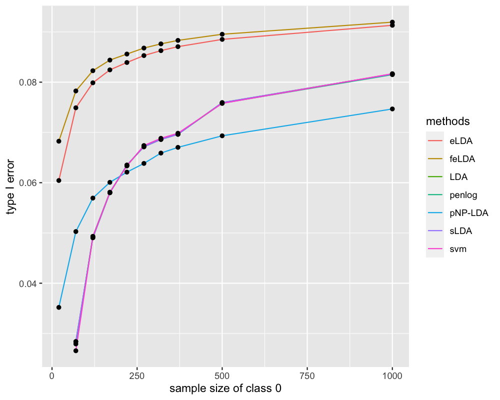
(c) Example 1b, type I error

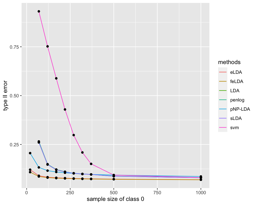
(d) Example 1b, type II error

Figure E.2: Examples 1c, 1c’ and 1c*, type I and type II error for competing methods with increasing dimension $p$ and different $\delta$’s. $\delta=0.1$ in Example 1c, $\delta=0.05$ in Example 1c’, and $\delta=0.01$ in Example 1c*.

(a) Example 1c, type I error

(b) Example 1c, type II error

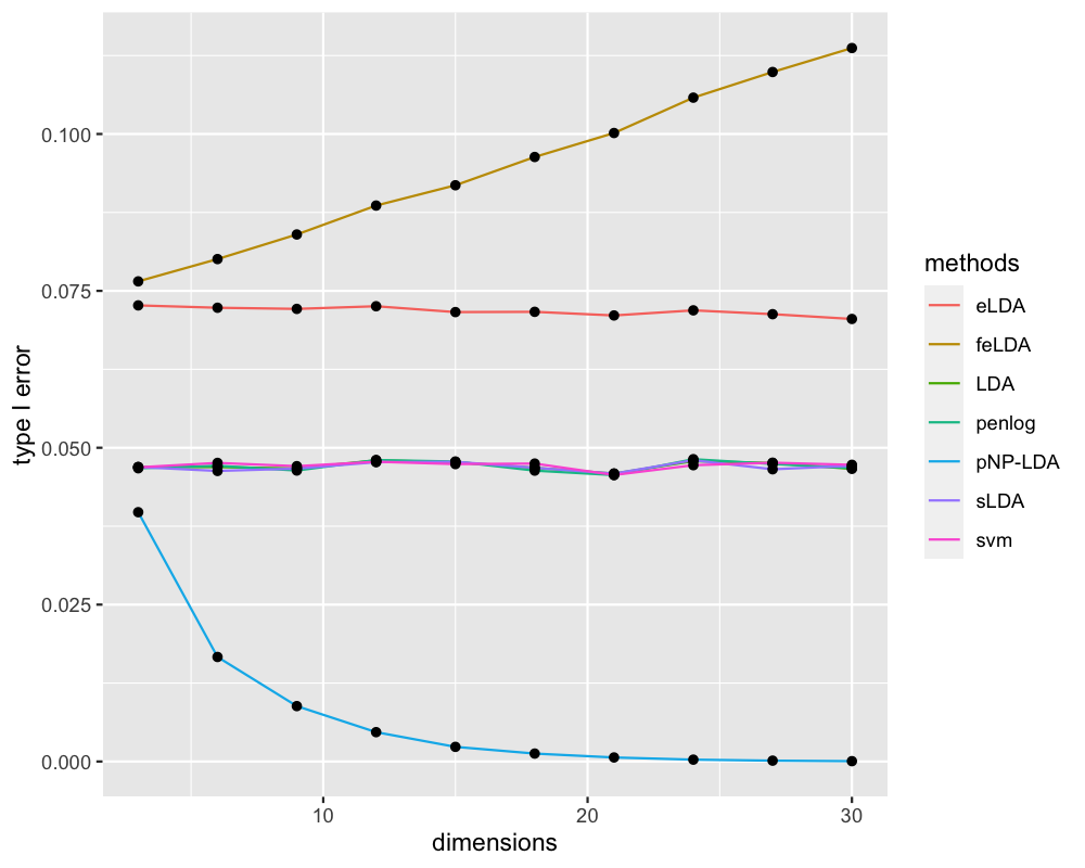
(c) Example 1c’, type I error

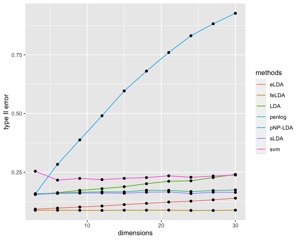
(d) Example 1c’, type II error

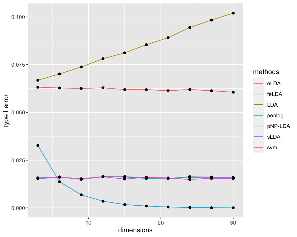
(e) Example 1c* type I error

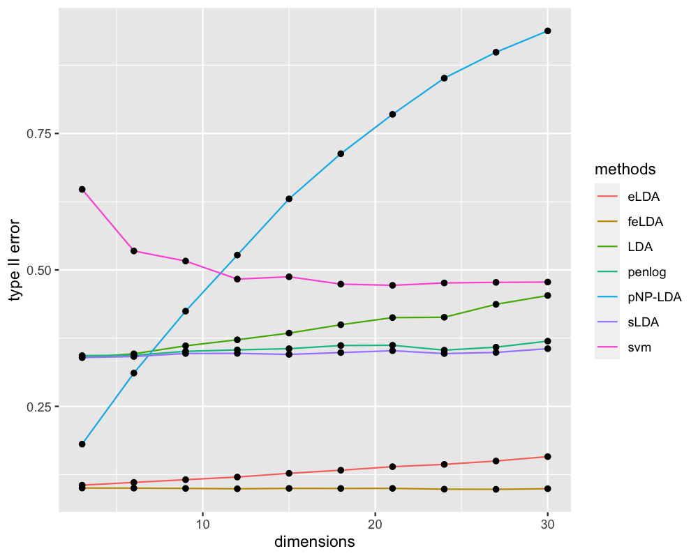
(f) Example 1c*, type II error

Figure E.3: Examples 1d and 1d’, imbalanced sample sizes with larger $n_{1}$. Type I and type II error for competing methods with increasing dimension $p$, but different $\delta$’s: $\delta=0.1$ in Example 1d and $\delta=0.05$ in Example 1d’.

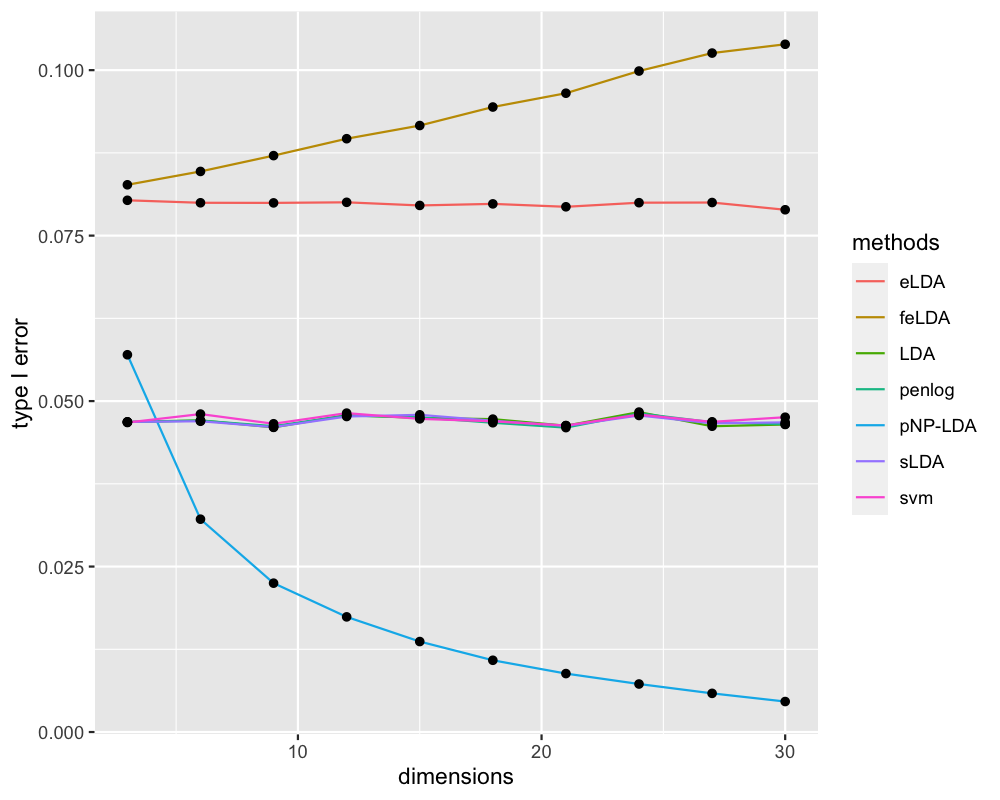
(a) Example 1d, type I error

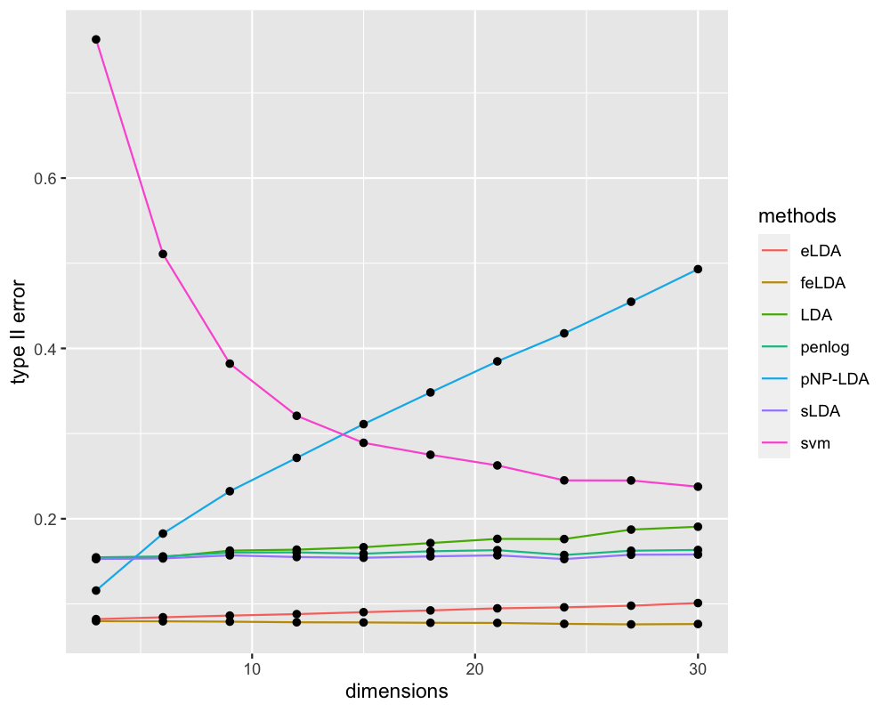
(b) Example 1d, type II error

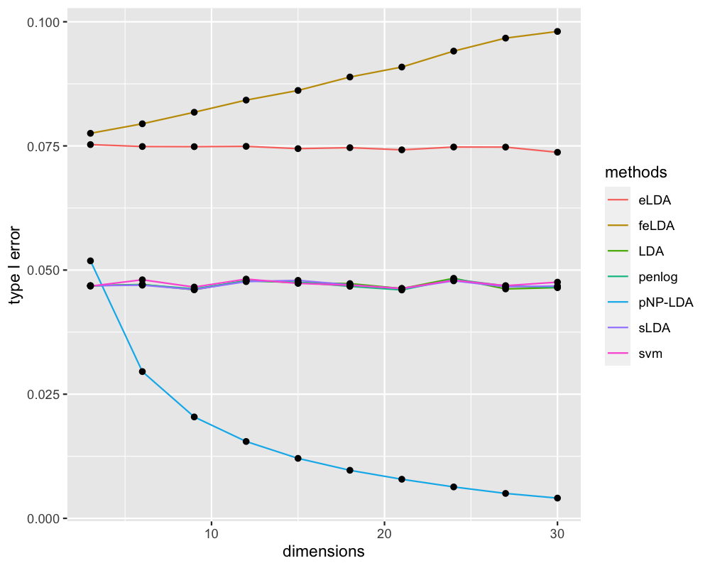
(c) Example 1d’, type I error

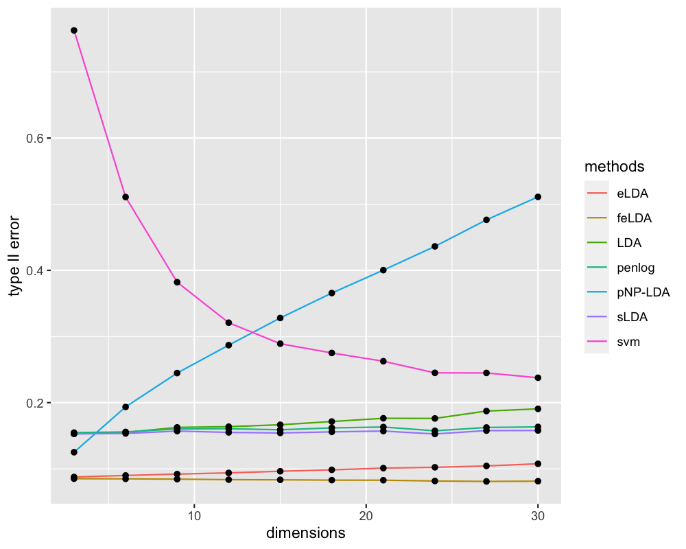
(d) Example 1d’, type II error

Table E.1: Examples 1a and 1b, violation rates over different $n_{0}$ and methods.

	Methods	$n_{0}=20$	$70$	$120$	$170$	$220$	$270$	$320$	$370$	$500$	$1000$
Example 1a	NP-lda	NA	.016	.047	.062	.071	.087	.074	.074	.078	.080
	NP-slda	NA	.016	.046	.062	.071	.086	.074	.074	.077	.079
	NP-penlog	NA	.018	.050	.064	.075	.096	.071	.071	.084	.078
	NP-svm	NA	.020	.045	.064	.077	.084	.068	.064	.082	.084
	pNP-lda	.000	.000	.004	.004	.002	.001	.001	.002	.002	.007
	elda	.091	.084	.108	.105	.103	.104	.104	.100	.101	.081
	felda	.220	.144	.145	.138	.134	.141	.141	.126	.121	.100
Example 1b	NP-lda	NA	.017	.043	.055	.072	.090	.078	.069	.078	.078
	NP-slda	NA	.017	.043	.056	.072	.090	.075	.069	.077	.078
	NP-penlog	NA	.016	.047	.063	.076	.091	.075	.072	.084	.074
	NP-svm	NA	.022	.058	.066	.072	.089	.070	.065	.082	.075
	pNP-lda	.028	.015	.012	.010	.005	.005	.003	.005	.002	.000
	elda	.083	.087	.090	.095	.095	.090	.099	.102	.101	.091
	felda	.138	.122	.112	.118	.122	.121	.121	.122	.121	.112

Table E.2: Examples 1c, 1c’ and 1c*, violation rates over different $p$ and methods.

	Methods	$p=3$	$6$	$9$	$12$	$15$	$18$	$21$	$24$	$27$	$30$
Example 1c $\delta=0.1$	NP-lda	.044	.039	.039	.045	.058	.046	.035	.049	.044	.048
	NP-slda	.045	.033	.037	.050	.047	.043	.034	.045	.038	.041
	NP-penlog	.037	.042	.035	.056	.050	.044	.031	.049	.043	.041
	NP-svm	.041	.040	.041	.044	.041	.042	.043	.039	.035	.048
	pNP-lda	.001	.000	.000	.000	.000	.000	.000	.000	.000	.000
	elda	.105	.091	.084	.107	.104	.079	.105	.099	.082	.082
	felda	.147	.206	.274	.362	.435	.548	.597	.712	.790	.817
Example 1c’ $\delta=0.05$	NP-lda	.044	.039	.039	.045	.058	.046	.035	.049	.044	.048
	NP-slda	.045	.033	.037	.050	.047	.043	.034	.045	.038	.041
	NP-penlog	.037	.042	.035	.056	.050	.044	.031	.049	.043	.041
	NP-svm	.041	.040	.041	.044	.041	.042	.043	.039	.035	.048
	pNP-lda	.001	.000	.000	.000	.000	.000	.000	.000	.000	.000
	elda	.061	.049	.043	.052	.046	.042	.057	.054	.044	.044
	felda	.087	.115	.161	.260	.431	.410	.472	.599	.679	.732
Example 1c* $\delta=0.01$	NP-lda	.001	.001	.000	.004	.002	.000	.000	.000	.002	.001
	NP-slda	.001	.001	.001	.003	.004	.000	.002	.000	.000	.001
	NP-penlog	.001	.001	.000	.003	.004	.000	.001	.000	.001	.001
	NP-svm	.000	.002	.001	.002	.000	.002	.000	.000	.001	.001
	pNP-lda	.000	.000	.000	.000	.000	.000	.000	.000	.000	.000
	elda	.014	.007	.008	.009	.003	.011	.011	.016	.010	.010
	felda	.025	.032	.053	.100	.146	.188	.259	.361	.436	.530

Figure E.4: Examples 2a and 2b, type I and type II error for competing methods with increasing dimension $p$. Example 2a has balanced sample sizes and Example 2b has imbalanced sample sizes.

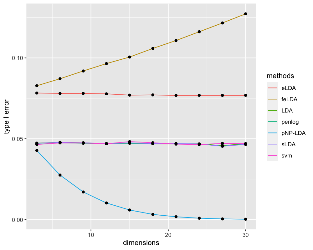
(a) Example 2a, type I error

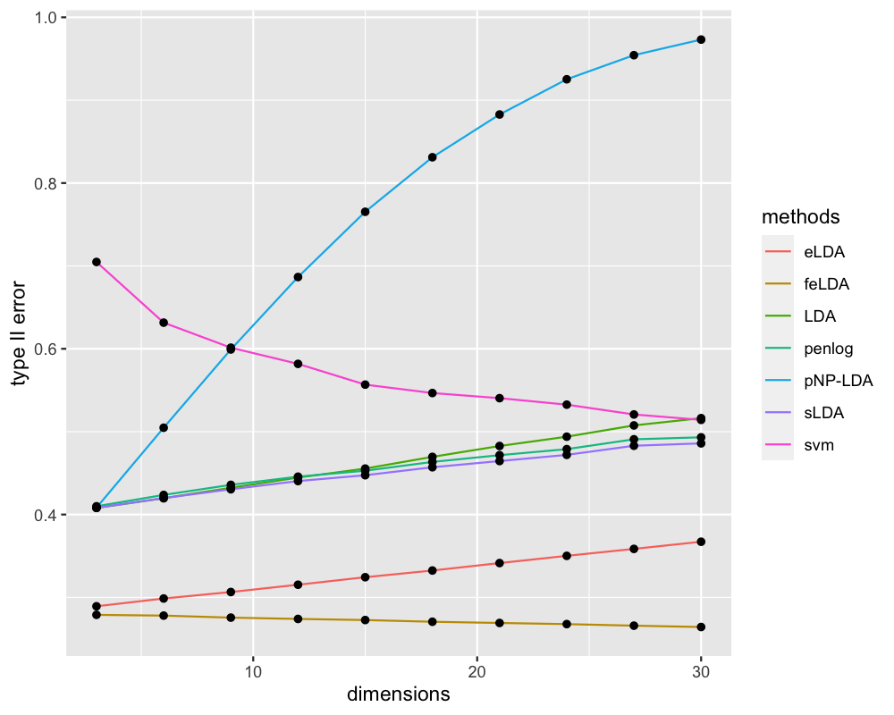
(b) Example 2a type II error

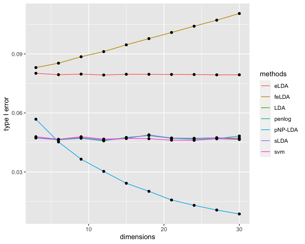
(c) Example 2b, type I error

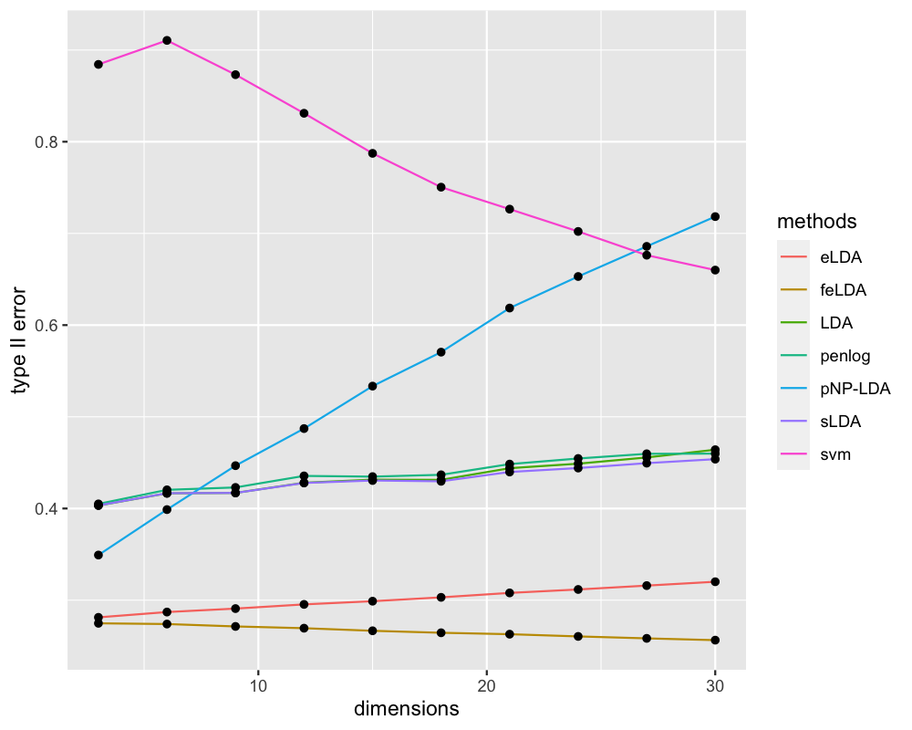
(d) Example 2b, type II error

E.2 An extra example on t-distributions

Example 3. The setting is the same as Example 1a in Section 6 in the main text, except that instead of from multivariate Gaussian distributions, data are generated from multivariate t-distributions with degrees of freedom 4.

Example 3 helps provide a broader understanding of the newly proposed classifiers under non-Gaussian distributions. Figure E.5 depicts type I and type II errors, and Table E.3 summarizes the observed violation rates. We have two observations as follows: 1) among pNP-lda, elda and felda, which are implementable for all sample sizes, elda and felda clearly dominate pNP-lda. elda and felda have the type I error bounded under $\alpha$ and enjoy much smaller type II errors comparing to pNP-lda; 2) comparing elda and felda with other umbrella algorithm based NP classifiers, we observe that when sample size of class 0 is very small (in the current setting, less than 220), the umbrella algorithm based classifiers either cannot be implemented ($n_{0}=20$) or have much worse type II errors than elda and felda. As the sample size further increases, the performances of most umbrella algorithm based classifiers begin to catch up and eventually outperform elda and felda. We believe this phenomenon is due to the fine calibration of the LDA model in the development of elda and felda, which leads to conservative results in heavy-tail distribution settings. On the other hand, the nonparametric NP umbrella algorithm does not rely on any distributional assumptions and benefit from larger sample sizes.

Figure E.5: Example 3, type I and type II error for competing methods with increasing and balanced sample sizes

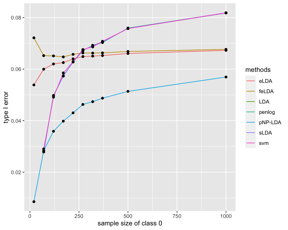
(a) Example 3, Type I error

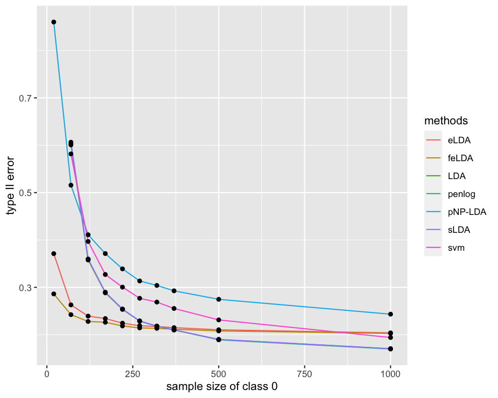
(b) Example 3 Type II error

Table E.3: Example 3, violation rates over different $n_{0}$ and methods.

	Methods	$n_{0}=20$	$70$	$120$	$170$	$220$	$270$	$320$	$370$	$500$	$1000$
Example 3	NP-lda	NA	.024	.067	.064	.068	.074	.073	.078	.073	.057
	NP-slda	NA	.024	.071	.062	.069	.078	.069	.076	.074	.056
	NP-penlog	NA	.021	.061	.059	.069	.077	.073	.074	.075	.058
	NP-svm	NA	.026	.063	.066	.066	.084	.065	.080	.081	.068
	pNP-lda	.000	.001	.000	.000	.000	.000	.000	.000	.000	.000
	elda	.075	.026	.009	.006	.003	.001	.003	.001	.000	.000
	felda	.191	.043	.017	.011	.004	.001	.003	.001	.001	.000

E.3 Lung cancer dataset continued

For the lung cancer dataset we explored in the real data section, we selected another set of parameters $\alpha=0.1$, and $\delta=0.4$ for a comparison among all five methods, including the umbrella algorithm based NP methods. We present the results in Table E.4. We observe that, elda dominates NP-slda, NP-penlog, and NP-svm in both the type I and the type II errors. pNP-lda again produces a type I error of 0 and a type II error of 1: not informative at all. elda outperforms all other competing methods.

Table E.4: Lung cancer dataset

		NP-slda	NP-penlog	NP-svm	pNP-lda	elda
$\alpha=0.1$ $\delta=0.4$	type I error	.083	.078	.081	.000	.031
	type II error	.015	.026	.022	1.000	.013
	observed violation rate	.49	.45	.46	.00	.28

References

• Bloemendal et al. (2014) Bloemendal, A., L. Erdős, A. Knowles, H.-T. Yau, and J. Yin (2014). Isotropic local laws for sample covariance and generalized wigner matrices. Electronic Journal of Probability 19, 1–53.
• Bloemendal et al. (2016) Bloemendal, A., A. Knowles, H.-T. Yau, and J. Yin (2016). On the principal components of sample covariance matrices. Probability theory and related fields 164(1-2), 459–552.
• Cai and Zhang (2019) Cai, T. and L. Zhang (2019). High dimensional linear discriminant analysis: optimality, adaptive algorithm and missing data. Journal of the Royal Statistical Society: Series B (Statistical Methodology) 81(4), 675–705.
• Cai and Zhang (2021) Cai, T. and L. Zhang (2021). A convex optimization approach to high-dimensional sparse quadratic discriminant analysis. The Annals of Statistics 49(3), 1537–1568.
• Cannon et al. (2002) Cannon, A., J. Howse, D. Hush, and C. Scovel (2002). Learning with the neyman-pearson and min-max criteria. Los Alamos National Laboratory, Tech. Rep. LA-UR, 02–2951.
• Erdős et al. (2013) Erdős, L., A. Knowles, and H.-T. Yau (2013). Averaging fluctuations in resolvents of random band matrices. Ann. Henri Poincaré 14(8), 1837–1926.
• Fan et al. (2012) Fan, J., Y. Feng, and X. Tong (2012). A road to classification in high dimensional space: the regularized optimal affine discriminant. Journal of the Royal Statistical Society. Series B (Statistical Methodology) 74, 745–771.
• Fan et al. (2020) Fan, J., R. Li, C.-h. Zhang, and H. Zou (2020). Statistical Foundations of Data Science. Chapman & Hall.
• Fan and Song (2010) Fan, J. and R. Song (2010). Sure independence screening in generalized linear models with np-dimensionality. The Annals of Statistics 38(6), 3567–3604.
• Fan et al. (2015) Fan, Y., Y. Kong, D. Li, and Z. Zheng (2015). Innovated interaction screening for high-dimensional nonlinear classification. The Annals of Statistics 43(3), 1243–1272.
• Gordon et al. (2002) Gordon, G. J., R. V. Jensen, L.-L. Hsiao, S. R. Gullans, J. E. Blumenstock, S. Ramaswamy, W. G. Richards, D. J. Sugarbaker, and R. Bueno (2002). Translation of microarray data into clinically relevant cancer diagnostic tests using gene expression ratios in lung cancer and mesothelioma. Cancer research 62(17), 4963–4967.
• Hao et al. (2015) Hao, N., B. Dong, and J. Fan (2015). Sparsifying the fisher linear discriminant by rotation. Journal of the Royal Statistical Society Series B 72, 827–851.
• Hastie et al. (2009) Hastie, T., R. Tibshirani, and J. H. Friedman (2009). The Elements of Statistical Learning: Data Mining, Inference, and Prediction (2nd edition). Springer-Verlag Inc.
• James et al. (2014) James, G., D. Witten, T. Hastie, and R. Tibshirani (2014). An Introduction to Statistical Learning: with Applications in R. Springer Texts in Statistics. Springer New York.
• Jin and Wang (2016) Jin, J. and W. Wang (2016). Influential features pca for high dimensional clustering. The Annals of Statistics 44(6), 2323–2359.
• Li and Shao (2015) Li, Q. and J. Shao (2015). Sparse quadratic discriminant analysis for high dimensional data. Statistica Sinica, 457–473.
• Li et al. (2012) Li, R., W. Zhong, and L. Zhu (2012). Feature screening via distance correlation learning. Journal of the American Statistical Association 107(499), 1129–1139.
• Li and Lei (2018) Li, Y. and J. Lei (2018). Sparse subspace linear discriminant analysis. Statistics 52(4), 782–800.
• Mai et al. (2012) Mai, Q., H. Zou, and M. Yuan (2012). A direct approach to sparse discriminant analysis in ultra-high dimensions. Biometrika 99, 29–42.
• Mammen and Tsybakov (1999) Mammen, E. and A. Tsybakov (1999). Smooth discrimination analysis. Annals of Statistics 27, 1808–1829.
• Pan et al. (2016) Pan, R., H. Wang, and R. Li (2016). Ultrahigh-dimensional multiclass linear discriminant analysis by pairwise sure independence screening. Journal of the American Statistical Association 111(513), 169–179.
• Pan and Mai (2020) Pan, Y. and Q. Mai (2020). Efficient computation for differential network analysis with applications to quadratic discriminant analysis. Computational Statistics & Data Analysis 144, 106884.
• Polonik (1995) Polonik, W. (1995). Measuring mass concentrations and estimating density contour clusters–an excess mass approach. Annals of Statistics 23, 855–881.
• Rigollet and Tong (2011) Rigollet, P. and X. Tong (2011). Neyman-pearson classification, convexity and stochastic constraints. Journal of Machine Learning Research 12(Oct), 2831–2855.
• Scott (2019) Scott, C. (2019). A generalized neyman-pearson criterion for optimal domain adaptation. Proceedings of Machine Learning Research 93, 1–24.
• Scott and Nowak (2005) Scott, C. and R. Nowak (2005). A neyman-pearson approach to statistical learning. IEEE Transactions on Information Theory 51(11), 3806–3819.
• Shao et al. (2011) Shao, J., Y. Wang, X. Deng, and S. Wang (2011). Sparse linear discriminant analysis by thresholding for high dimensional data. Annals of Statistics 39, 1241–1265.
• Sifaou et al. (2020) Sifaou, H., A. Kammoun, and M.-S. Alouini (2020). High-dimensional linear discriminant analysis classifier for spiked covariance model. Journal of Machine Learning Research 21(112), 1–24.
• Su et al. (2001) Su, A. I., J. B. Welsh, L. M. Sapinoso, S. G. Kern, P. Dimitrov, H. Lapp, P. G. Schultz, S. M. Powell, C. A. Moskaluk, H. F. Frierson, et al. (2001). Molecular classification of human carcinomas by use of gene expression signatures. Cancer research 61(20), 7388–7393.
• Tian and Feng (2021) Tian, Y. and Y. Feng (2021). Neyman-pearson multi-class classification via cost-sensitive learning. arXiv:2111.04597.
• Tong (2013) Tong, X. (2013). A plug-in approach to neyman-pearson classification. Journal of Machine Learning Research 14(1), 3011–3040.
• Tong et al. (2018) Tong, X., Y. Feng, and J. J. Li (2018). Neyman-pearson classification algorithms and np receiver operating characteristics. Science Advances 4(2), eaao1659.
• Tong et al. (2020) Tong, X., L. Xia, J. Wang, and Y. Feng (2020). Neyman-pearson classification: parametrics and sample size requirement. Journal of Machine Learning Research 21, 1–18.
• Wang and Jiang (2018) Wang, C. and B. Jiang (2018). On the dimension effect of regularized linear discriminant analysis. Electronic Journal of Statistics 12, 2709–2742.
• Wang et al. (2021) Wang, W., J. Wu, and Z. Yao (2021). Phase transitions for high-dimensional quadratic discriminant analysis with rare and weak signals. arXiv preprint arXiv:2108.10802.
• Witten and Tibshirani (2012) Witten, D. and R. Tibshirani (2012). Penalized classification using fisher’s linear discriminant. Journal of the Royal Statistical Society Series B 73, 753–772.
• Yang and Cheng (2018) Yang, Q. and G. Cheng (2018). Quadratic discriminant analysis under moderate dimension. arXiv:1808.10065.
• Yousefi et al. (2010) Yousefi, M. R., J. Hua, C. Sima, and E. R. Dougherty (2010). Reporting bias when using real data sets to analyze classification performance. Bioinformatics 26(1), 68–76.
• Zhao et al. (2016) Zhao, A., Y. Feng, L. Wang, and X. Tong (2016). Neyman-pearson classification under high-dimensional settings. Journal of Machine Learning Research 17(213), 1–39.