Asymmetric error control under imperfect supervision: a label-noise-adjusted Neyman-Pearson umbrella algorithm

Shunan Yao Department of Mathematics, Dana and David Dornsife College of Letters, Arts and Sciences, University of Southern California. Bradley Rava Department of Data Sciences and Operations, Marshall School of Business, University of Southern California. Xin Tong Department of Data Sciences and Operations, Marshall School of Business, University of Southern California. To whom correspondence should be addressed. xint@marshall.usc.edu, gareth.james@marshall.usc.edu Gareth James Department of Data Sciences and Operations, Marshall School of Business, University of Southern California. To whom correspondence should be addressed. xint@marshall.usc.edu, gareth.james@marshall.usc.edu
Abstract

Label noise in data has long been an important problem in supervised learning applications as it affects the effectiveness of many widely used classification methods. Recently, important real-world applications, such as medical diagnosis and cybersecurity, have generated renewed interest in the Neyman-Pearson (NP) classification paradigm, which constrains the more severe type of error (e.g., the type I error) under a preferred level while minimizing the other (e.g., the type II error). However, there has been little research on the NP paradigm under label noise. It is somewhat surprising that even when common NP classifiers ignore the label noise in the training stage, they are still able to control the type I error with high probability. However, the price they pay is excessive conservativeness of the type I error and hence a significant drop in power (i.e., 1limit-from11- type II error). Assuming that domain experts provide lower bounds on the corruption severity, we propose the first theory-backed algorithm that adapts most state-of-the-art classification methods to the training label noise under the NP paradigm. The resulting classifiers not only control the type I error with high probability under the desired level but also improve power.

KEY WORDS: label noise, classification, Neyman-Pearson (NP) paradigm, type I error, umbrella algorithm.

1 Introduction

Most classification methods assume a perfectly labeled training dataset. Yet, it is estimated that in real-world databases around five percent of labels are incorrect (Orr, 1998; Redman, 1998). Labeling errors might come from insufficient guidance to human coders, poor data quality, or human mistakes in decisions, among others (Brazdil and Konolige, 1990; Hickey, 1996; Brodley and Friedl, 1999b). Specifically, in the medical field, a 2011 survey of more than 6,00060006{,}000 physicians found that half said they encountered diagnostic errors at least once a month (MacDonald, 2011). The existence of labeling errors in training data is often referred to as label noise, imperfect labels or imperfect supervision. It belongs to a more general data corruption problem, which refers to “anything which obscures the relationship between description and class” (Hickey, 1996).

The study of label noise in supervised learning has been a vibrant field in academia. On the empirical front, researchers have found that some statistical learning methods such as quadratic discriminant analysis (Lachenbruch, 1979) and k-NN (Okamoto and Yugami, 1997), can be greatly affected by label noise and have accuracy seriously reduced, while other methods, such as linear discriminant analysis (Lachenbruch, 1966), are more label noise tolerant. Moreover, one can modify AdaBoost (Cao et al., 2012), perceptron algorithm (Khardon and Wachman, 2007) and neural networks (Sukhbaatar and Fergus, 2014), so that they are more tolerant to label noise. Data cleansing techniques were also developed, such as in Guyon et al. (1996) and Brodley and Friedl (1999a). On the theoretical front, Natarajan et al. (2013) provided a guarantee for risk minimization in the setting of convex surrogates. Manwani and Sastry (2013) proved label noise tolerance of risk minimization for certain types of loss functions, and Ghosh et al. (2015) extended the result by considering more loss types. Liu and Tao (2016) proposed learning methods with importance-reweighting which can minimize the risk. Blanchard et al. (2016) studied intensely the class-conditional corruption model, a model that many works on label noise are based on. In particular, theoretical results about parameter estimation and consistency of classifiers under this model were presented in their work. Most recently, Cannings et al. (2020) derived innovative theory of excess risk for general classifiers.

In many classification settings, one type of error may have far worse consequences than the other. For example, a biomedical diagnosis/prognosis that misidentifies a benign tumor as malignant will cause distress and potentially unnecessary medical procedures, but the alternative, where a malignant tumor is classified as benign, will have far worse outcomes. Other related predictive applications include cybersecurity and finance. Despite great advances in the label-noise classification literature, to our knowledge, no classifier has been constructed to deal with this asymmetry in error importance under label noise so as to control the level of the more severe error type.

In this paper, we concentrate on the classification setting involving both mislabeled outcomes and error importance asymmetry. The Neyman-Pearson (NP) paradigm (Cannon et al., 2002; Scott and Nowak, 2005), which controls the false-negative rate (FNR, a.k.a., type I error111Note that type I error in our work is defined to be the conditional probability of misclassifying a 0 instance as class 1. Moreover, we code the more severe class as class 0. In the disease diagnosis example, the disease class would be class 0. ) under some desired level while minimizing the false-positive rate (FPR, a.k.a., type II error), provides a natural approach to this problem. However, to the best of our knowledge, there has been no work that studies how label noise issues affect the control of the more severe FNR. We show that if one trains a standard NP classifier on corrupted labels (e.g., the NP umbrella algorithm (Tong et al., 2018)), then the actual achieved FNR is far below the control target, resulting in a very high, and undesirable, FPR.

This problem motivates us to devise a new label-noise-adjusted umbrella algorithm that corrects for the labeling errors to produce a lower FPR while still controlling the FNR. The construction of such an algorithm is challenging because we must identify the optimal correction level without any training data from the uncorrupted distribution. To address this challenge, we employ a common class-conditional noise model and derive the population-level difference between the type I errors of the true and corrupted labels. Based on this difference, we propose a sample-based correction term that, even without observing any uncorrupted labels, can correctly adjust the NP umbrella algorithm to significantly reduce the FPR while still controlling the FNR.

Our approach has several advantages. First, it is the first theory-backed methodology in the label noise setting to control population-level type I error (i.e., FNR) regarding the true labels. Concretely, we can show analytically that the new algorithm produces classifiers that have a high probability of controlling the FNR below the desired threshold with a FPR lower than that provided by the original NP umbrella algorithm. Second, when there are no labeling errors, our new algorithm reduces to the original NP algorithm. Finally, we demonstrate on both simulated and real-world data, that under the NP paradigm the new algorithm dominates the original unadjusted one and competes favorably against existing methods which handle label noise in classification.

The rest of the paper is organized as follows. In Section 2, we introduce some notation and a corruption model to study the label noise. In Section 3, we demonstrate the ineffectiveness of the original NP umbrella algorithm under label noise and propose a new label-noise-adjusted version. The validity and the high-probability type I error control property of the new algorithm are established in Section 4. Simulation and real data analysis are conducted in Section 5, followed by a Discussion section. All proofs, additional numerical results, and technical results are relegated to the Appendix.

2 Notation and Corruption Model

Let (X,Y,Y~)𝑋𝑌~𝑌(X,Y,\tilde{Y}) be a random triplet, where X𝒳IRd𝑋𝒳superscriptIR𝑑X\in\mathcal{X}\subset{\rm I}\kern-1.43994pt{\rm R}^{d} represents features, Y{0,1}𝑌01Y\in\{0,1\} encodes the true class labels and Y~{0,1}~𝑌01\tilde{Y}\in\{0,1\} the corrupted ones. Note that in our setting, we cannot observe Y𝑌Y; the observations come from (X,Y~)𝑋~𝑌(X,\tilde{Y}). Denote X0X(Y=0)superscript𝑋0conditional𝑋𝑌0X^{0}\triangleq X\mid(Y=0) and X1X(Y=1)superscript𝑋1conditional𝑋𝑌1X^{1}\triangleq X\mid(Y=1). Similarly, denote X~0X(Y~=0)superscript~𝑋0conditional𝑋~𝑌0\tilde{X}^{0}\triangleq X\mid(\tilde{Y}=0) and X~1X(Y~=1)superscript~𝑋1conditional𝑋~𝑌1\tilde{X}^{1}\triangleq X\mid(\tilde{Y}=1). Denote by IPIP{\rm I}\kern-1.43994pt{\rm P} and IEIE{\rm I}\kern-1.43994pt{\rm E} generic probability measure and expectation whose meanings depend on the context. For any Borel set A𝒳𝐴𝒳A\subset\mathcal{X}, we denote

P0(A)subscript𝑃0𝐴\displaystyle P_{0}(A) =IP(XA|Y=0), P1(A)=IP(XA|Y=1),formulae-sequenceabsentIP𝑋conditional𝐴𝑌0 subscript𝑃1𝐴IP𝑋conditional𝐴𝑌1\displaystyle={\rm I}\kern-1.43994pt{\rm P}(X\in A|Y=0)\,,\text{ }P_{1}(A)={\rm I}\kern-1.43994pt{\rm P}(X\in A|Y=1)\,,
P~0(A)subscript~𝑃0𝐴\displaystyle\tilde{P}_{0}(A) =IP(XA|Y~=0), P~1(A)=IP(XA|Y~=1).formulae-sequenceabsentIP𝑋conditional𝐴~𝑌0 subscript~𝑃1𝐴IP𝑋conditional𝐴~𝑌1\displaystyle={\rm I}\kern-1.43994pt{\rm P}(X\in A|\tilde{Y}=0)\,,\text{ }\tilde{P}_{1}(A)={\rm I}\kern-1.43994pt{\rm P}(X\in A|\tilde{Y}=1)\,.

Then, we denote by F0,F1,F~0subscript𝐹0subscript𝐹1subscript~𝐹0F_{0}\,,F_{1}\,,\tilde{F}_{0} and F~1subscript~𝐹1\tilde{F}_{1} their respective distribution functions and by f0,f1,f~0subscript𝑓0subscript𝑓1subscript~𝑓0f_{0}\,,f_{1}\,,\tilde{f}_{0} and f~1subscript~𝑓1\tilde{f}_{1} the density functions, assuming they exist. Moreover, for a measurable function T:𝒳IR:𝑇𝒳IRT:\mathcal{X}\rightarrow{\rm I}\kern-1.43994pt{\rm R}, we denote, for any zIR𝑧IRz\in{\rm I}\kern-1.43994pt{\rm R},

F0T(z)subscriptsuperscript𝐹𝑇0𝑧\displaystyle F^{T}_{0}(z) =P0(T(X)z), F1T(z)=P1(T(X)z),formulae-sequenceabsentsubscript𝑃0𝑇𝑋𝑧 subscriptsuperscript𝐹𝑇1𝑧subscript𝑃1𝑇𝑋𝑧\displaystyle=P_{0}(T(X)\leq z)\,,\text{ }F^{T}_{1}(z)=P_{1}(T(X)\leq z)\,,
F~0T(z)subscriptsuperscript~𝐹𝑇0𝑧\displaystyle\tilde{F}^{T}_{0}(z) =P~0(T(X)z), F~1T(z)=P~1(T(X)z).formulae-sequenceabsentsubscript~𝑃0𝑇𝑋𝑧 subscriptsuperscript~𝐹𝑇1𝑧subscript~𝑃1𝑇𝑋𝑧\displaystyle=\tilde{P}_{0}(T(X)\leq z)\,,\text{ }\tilde{F}^{T}_{1}(z)=\tilde{P}_{1}(T(X)\leq z)\,.

Since the effect of, and adjustment to, the label noise depend on the type and severity of corruption, we need to specify a corruption model to work with. Our choice for this work is the class-conditional noise (contamination) model, which is specified in the next assumption.

Assumption 1.

There exist constants m0,m1[0,1]subscript𝑚0subscript𝑚101m_{0},m_{1}\in[0,1] such that for any Borel set A𝒳𝐴𝒳A\subset\mathcal{X},

P~0(A)=m0P0(A)+(1m0)P1(A)  and  P~1(A)=m1P0(A)+(1m1)P1(A).subscript~𝑃0𝐴subscript𝑚0subscript𝑃0𝐴1subscript𝑚0subscript𝑃1𝐴  and  subscript~𝑃1𝐴subscript𝑚1subscript𝑃0𝐴1subscript𝑚1subscript𝑃1𝐴\displaystyle\tilde{P}_{0}(A)=m_{0}P_{0}(A)+(1-m_{0})P_{1}(A)\,\text{ }\text{ and }\text{ }\tilde{P}_{1}(A)=m_{1}P_{0}(A)+(1-m_{1})P_{1}(A)\,. (1)

Furthermore, assume m0>m1subscript𝑚0subscript𝑚1m_{0}>m_{1} but both quantities can be unknown. Moreover, let m0#,m1#[0,1]superscriptsubscript𝑚0#superscriptsubscript𝑚1#01m_{0}^{\#},m_{1}^{\#}\in[0,1] be known constants such that m0#m0superscriptsubscript𝑚0#subscript𝑚0m_{0}^{\#}\geq m_{0} and m1#m1superscriptsubscript𝑚1#subscript𝑚1m_{1}^{\#}\leq m_{1}.

Example 1.

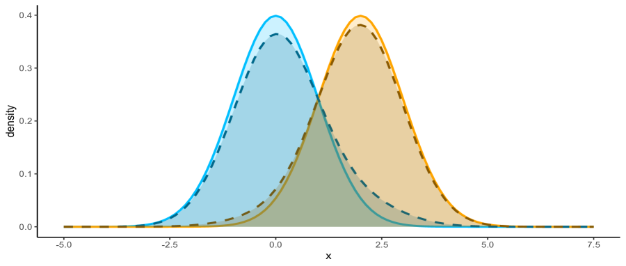
[An example of Assumption 1] Let X0𝒩(μ0,σ2)similar-tosuperscript𝑋0𝒩subscript𝜇0superscript𝜎2X^{0}\sim\mathcal{N}(\mu_{0},\sigma^{2}) and X1𝒩(μ1,σ2)similar-tosuperscript𝑋1𝒩subscript𝜇1superscript𝜎2X^{1}\sim\mathcal{N}(\mu_{1},\sigma^{2}), where μ0,μ1IRsubscript𝜇0subscript𝜇1IR\mu_{0},\mu_{1}\in{\rm I}\kern-1.43994pt{\rm R} and σ>0𝜎0\sigma>0. Then F~0(z)=m0Φ(zμ0σ)+(1m0)Φ(zμ1σ)subscript~𝐹0𝑧subscript𝑚0Φ𝑧subscript𝜇0𝜎1subscript𝑚0Φ𝑧subscript𝜇1𝜎\tilde{F}_{0}(z)=m_{0}\Phi(\frac{z-\mu_{0}}{\sigma})+(1-m_{0})\Phi(\frac{z-\mu_{1}}{\sigma}) and F~1(z)=m1Φ(zμ0σ)+(1m1)Φ(zμ1σ)subscript~𝐹1𝑧subscript𝑚1Φ𝑧subscript𝜇0𝜎1subscript𝑚1Φ𝑧subscript𝜇1𝜎\tilde{F}_{1}(z)=m_{1}\Phi(\frac{z-\mu_{0}}{\sigma})+(1-m_{1})\Phi(\frac{z-\mu_{1}}{\sigma}), where Φ()Φ\Phi(\cdot) is the distribution function of 𝒩(0,1)𝒩01\mathcal{N}(0,1). With the choice of μ0=0subscript𝜇00\mu_{0}=0, μ1=1subscript𝜇11\mu_{1}=1, σ=1𝜎1\sigma=1, m0=0.9subscript𝑚00.9m_{0}=0.9, and m1=0.05subscript𝑚10.05m_{1}=0.05, the density functions f0subscript𝑓0f_{0}, f~0subscript~𝑓0\tilde{f}_{0}, f1subscript𝑓1f_{1} and f~1subscript~𝑓1\tilde{f}_{1} are plotted in Figure 1.

Refer to caption
Figure 1: Density plots in Example 1. True (lighter and solid) and corrupted (darker and dashed).

Note that equation (1) specifies perhaps the simplest model for label noise in supervised learning. Here, m0subscript𝑚0m_{0} and m1subscript𝑚1m_{1} represent the severity of corruption levels. Concretely, m0subscript𝑚0m_{0} can be interpreted as the proportion of true 00 observations among corrupted 00 observations, and m1subscript𝑚1m_{1} the proportion of true 00 observations among corrupted 111 observations. The assumption m0>m1subscript𝑚0subscript𝑚1m_{0}>m_{1} means that corrupted class 00 resembles true class 00 more than corrupted class 111 does, and that corrupted class 111 resembles true class 111 more than corrupted class 00 does. However, this assumption does not mean that corrupted class 00 resembles true class 00 more than it resembles true class 111 (i.e, m0>1/2subscript𝑚012m_{0}>1/2) or that corrupted class 111 resembles true class 111 more than it resembles true class 00 (i.e., m1<1/2subscript𝑚112m_{1}<1/2). Note that by the way our model is written, m0=1subscript𝑚01m_{0}=1 and m1=0subscript𝑚10m_{1}=0 correspond to the no label noise situation; as such, the roles of m0subscript𝑚0m_{0} and m1subscript𝑚1m_{1} are not symmetric. Hence, the assumptions m0#m0superscriptsubscript𝑚0#subscript𝑚0m_{0}^{\#}\geq m_{0} and m1#m1superscriptsubscript𝑚1#subscript𝑚1m_{1}^{\#}\leq m_{1} mean that we know some lower bounds of the corruption levels.

The class-conditional label noise model has been widely adopted in the literature (Natarajan et al., 2013; Liu and Tao, 2016; Blanchard et al., 2016). We note here that the assumption m0>m1subscript𝑚0subscript𝑚1m_{0}>m_{1} aligns with the total noise assumption π0+π1<1subscript𝜋0subscript𝜋11\pi_{0}+\pi_{1}<1 in Blanchard et al. (2016) as π0subscript𝜋0\pi_{0} and π1subscript𝜋1\pi_{1} in their work correspond to 1m01subscript𝑚01-m_{0} and m1subscript𝑚1m_{1} in Assumption 1, respectively. In Natarajan et al. (2013) and Liu and Tao (2016), the label noise was modeled through the label flipping probabilities: μi=IP(Y~=1i|Y=i)subscript𝜇𝑖IP~𝑌1conditional𝑖𝑌𝑖\mu_{i}={\rm I}\kern-1.43994pt{\rm P}(\tilde{Y}=1-i|Y=i), i=0,1𝑖01i=0,1. This alternative formulation is related to our formulation via Bayes’ rule. An in-depth study of the class-conditional label noise model, including mutual irreducibility and identifiability, was presented in Blanchard et al. (2016). Moreover, Blanchard et al. (2016) developed a noisy label trained classifier based on weighted cost-sensitive surrogate loss and established its consistency. Similarly, Natarajan et al. (2013) provided two methods to train classifiers, both relying on classification-calibrated surrogate loss; bounds for respective excess risks of these two methods were also given. Moreover, Liu and Tao (2016) proposed an importance reweighting method and extended the result in Natarajan et al. (2013) to all surrogate losses. Other than Blanchard et al. (2016), which briefly discussed the NP paradigm at the population level, in all aforementioned papers, though loss functions vary, the goal of classification is to minimize the overall risk. Our work focuses on the NP paradigm. Moreover, we focus on high probability control on the type I error based on finite samples, in contrast to asymptotic results in the literature.

In this work, we take the perspective that the domain experts can provide under-estimates of corruption levels. In the literature, there are existing methods to estimate these levels. For example, Liu and Tao (2016) and Blanchard et al. (2016) developed methods to estimate πisubscript𝜋𝑖\pi_{i}’s and μisubscript𝜇𝑖\mu_{i}’s, and showed consistency of their estimators. In numerical studies, we apply the method in Liu and Tao (2016) to estimate m0subscript𝑚0m_{0} and m1subscript𝑚1m_{1}222Note that though their method targets at μisubscript𝜇𝑖\mu_{i}’s, estimates of misubscript𝑚𝑖m_{i}’s in equation (1) can be constructed from those of μisubscript𝜇𝑖\mu_{i}’s by the Bayes’ theorem.. Numerical evidence shows that using these estimators in our proposed algorithm fails to establish a high probability control of the true type I error. In fact, even using consistent and unbiased estimators of m0subscript𝑚0m_{0} and m1subscript𝑚1m_{1} as inputs of our proposed algorithm would not be able to control the true type I error with high probability. One such case is demonstrated in Simulation 8 of the Appendix, where estimators for m0subscript𝑚0m_{0} and m1subscript𝑚1m_{1} are normally distributed and centered at the true values. To have high probability control on the true type I error, we do need the “under-estimates” of corruption levels as in Assumption 1.

3 Methodology

In this section, we first formally introduce the Neyman-Pearson (NP) classification paradigm and review the NP umbrella algorithm (Tong et al., 2018) for the uncorrupted label scenario (Section 3.1). Then we provide an example demonstrating that in the presence of label noise, naively implementing the NP umbrella algorithm leads to excessively conservative type I error. i.e., type I error much smaller than the control target α𝛼\alpha. We analyze and capitalize on this phenomenon, and present new noise-adjusted versions of the NP umbrella algorithm, Algorithm 1 for known corruption levels (Section 3.2) and Algorithm 1#superscript1#1^{\#} for unknown corruption levels (Section 3.3). Algorithm 1 can be considered as a special case of Algorithm 1#superscript1#1^{\#}: m0#=m0superscriptsubscript𝑚0#subscript𝑚0m_{0}^{\#}=m_{0} and m1#=m1superscriptsubscript𝑚1#subscript𝑚1m_{1}^{\#}=m_{1}.

A few additional notations are introduced to facilitate our discussion. A classifier ϕ:𝒳{0,1}:italic-ϕ𝒳01\phi:\mathcal{X}\rightarrow\{0,1\} maps from the feature space to the label space. The (population-level) type I and II errors of ϕ()italic-ϕ\phi(\cdot) regarding the true labels (a.k.a., true type I and II errors) are respectively R0(ϕ)=P0(ϕ(X)Y)subscript𝑅0italic-ϕsubscript𝑃0italic-ϕ𝑋𝑌R_{0}(\phi)=P_{0}(\phi(X)\neq Y) and R1(ϕ)=P1(ϕ(X)Y)subscript𝑅1italic-ϕsubscript𝑃1italic-ϕ𝑋𝑌R_{1}(\phi)=P_{1}(\phi(X)\neq Y). The (population-level) type I and II errors of ϕ()italic-ϕ\phi(\cdot) regarding the corrupted labels (a.k.a., corrupted type I and II errors) are respectively R~0(ϕ)=P~0(ϕ(X)Y~)subscript~𝑅0italic-ϕsubscript~𝑃0italic-ϕ𝑋~𝑌\tilde{R}_{0}(\phi)=\tilde{P}_{0}(\phi(X)\neq\tilde{Y}) and R~1(ϕ)=P~1(ϕ(X)Y~)subscript~𝑅1italic-ϕsubscript~𝑃1italic-ϕ𝑋~𝑌\tilde{R}_{1}(\phi)=\tilde{P}_{1}(\phi(X)\neq\tilde{Y}). In verbal discussion in this paper, type I error without any suffix refers to type I error regarding the true labels.

3.1 The NP umbrella algorithm without label noise

The NP paradigm (Cannon et al., 2002; Scott and Nowak, 2005) aims to mimic the NP oracle

ϕαargminϕ:R0(ϕ)αR1(ϕ),subscriptsuperscriptitalic-ϕ𝛼subscriptargmin:italic-ϕsubscript𝑅0italic-ϕ𝛼subscript𝑅1italic-ϕ\phi^{*}_{{\alpha}}\in\operatorname*{arg\,min}_{\phi:\ R_{0}(\phi)\leq{\alpha}}R_{1}(\phi)\,,

where α(0,1)𝛼01\alpha\in(0,1) is a user-specified level that reflects the priority towards the type I error. In practice, with or without label noise, based on training data of finite sample size, it is usually impossible to ensure R0()αsubscript𝑅0𝛼R_{0}(\cdot)\leq\alpha almost surely. Instead, we aim to control the type I error with high probability. Recently, the NP umbrella algorithm Tong et al. (2018) has attracted significant attention333At the time of writing, the NP umbrella package has been downloaded over 35,0003500035{,}000 times.. This algorithm works in conjunction with any score based classification method (e.g., logistic regression, support vector machines, or random forest) to compress a d𝑑d-dimensional feature measurement to a 111-dimensional score, and then threshold the score to classify. Specifically, given a (score based) classification method, the NP umbrella algorithm uses a model-free order statistics approach to decide the threshold, attaining a high probability control on type I error with minimum type II error for that method. Moreover, when coupling with a classification method that matches the underlying data distribution, the NP umbrella algorithm also achieves a diminishing excess type II error, i.e., R1(ϕ^α)R1(ϕα)0subscript𝑅1subscript^italic-ϕ𝛼subscript𝑅1subscriptsuperscriptitalic-ϕ𝛼0R_{1}(\hat{\phi}_{\alpha})-R_{1}(\phi^{*}_{\alpha})\rightarrow 0. For example, Tong et al. (2020) showed that under a linear discriminant analysis (LDA) model, an LDA classifier with the score threshold determined by the NP umbrella algorithm satisfies both the control on type I error and a diminishing excess type II error444These two properties together were coined as the NP oracle inequalities by Rigollet and Tong (2011). Classifiers with these properties were constructed with non-parametric assumptions in Tong (2013) and Zhao et al. (2016). . Next we will review the implementation of the NP umbrella algorithm.

Let 𝒮0={Xj0}j=1M0superscript𝒮0superscriptsubscriptsuperscriptsubscript𝑋𝑗0𝑗1subscript𝑀0\mathcal{S}^{0}=\{X_{j}^{0}\}_{j=1}^{M_{0}} and 𝒮1={Xj1}j=1M1superscript𝒮1superscriptsubscriptsuperscriptsubscript𝑋𝑗1𝑗1subscript𝑀1\mathcal{S}^{1}=\{X_{j}^{1}\}_{j=1}^{M_{1}}, respectively be the uncorrupted observations in classes 0 and 1, where M0subscript𝑀0M_{0} and M1subscript𝑀1M_{1} are the number of observations from each class555Note that the uncorrupted data 𝒮0superscript𝒮0\mathcal{S}^{0} and 𝒮1superscript𝒮1\mathcal{S}^{1} are not available in our present label noise setting and we only use them here for review purposes.. Then, given a classification method (i.e., base algorithm, e.g., logistic regression), the NP umbrella algorithm is implemented by randomly splitting the class 0 data 𝒮0superscript𝒮0\mathcal{S}^{0} into two parts: 𝒮b0subscriptsuperscript𝒮0b\mathcal{S}^{0}_{\text{b}} and 𝒮t0subscriptsuperscript𝒮0t\mathcal{S}^{0}_{\text{t}}. The first part, 𝒮b0subscriptsuperscript𝒮0b\mathcal{S}^{0}_{\text{b}}, together with 𝒮1superscript𝒮1\mathcal{S}^{1}, is used to train the base algorithm, while the second part 𝒮t0subscriptsuperscript𝒮0t\mathcal{S}^{0}_{\text{t}} determines the threshold candidates. Specifically, we train a base algorithm with scoring function T^()^𝑇\hat{T}(\cdot) (e.g., the sigmoid function in logistic regression) using 𝒮b0𝒮1subscriptsuperscript𝒮0bsuperscript𝒮1\mathcal{S}^{0}_{\text{b}}\,\cup\,\mathcal{S}^{1}, apply T^()^𝑇\hat{T}(\cdot) on 𝒮t0subscriptsuperscript𝒮0t\mathcal{S}^{0}_{\text{t}} (|𝒮t0|=nsubscriptsuperscript𝒮0t𝑛|\mathcal{S}^{0}_{\text{t}}|=n) to get threshold candidates {t1,,tn}subscript𝑡1subscript𝑡𝑛\{t_{1},\ldots,t_{n}\}, and sort them in an increasing order {t(1),,t(n)}subscript𝑡1subscript𝑡𝑛\{t_{(1)},\ldots,t_{(n)}\}. Then the NP umbrella algorithm proposes classifier ϕ^k()=1I{T^()>t(k)}subscript^italic-ϕsubscript𝑘1I^𝑇subscript𝑡subscript𝑘\hat{\phi}_{k_{*}}(\cdot)={\rm 1}\kern-1.92004pt{\rm I}\{\hat{T}(\cdot)>t_{(k_{*})}\}, where

k=min{k{1,,n}:j=kn(nj)(1α)jα(nj)δ},subscript𝑘minconditional-set𝑘1𝑛superscriptsubscript𝑗𝑘𝑛binomial𝑛𝑗superscript1𝛼𝑗superscript𝛼𝑛𝑗𝛿k_{*}=\text{min}\left\{k\in\{1,\ldots,n\}:\sum_{j=k}^{n}{n\choose j}(1-{\alpha})^{j}{\alpha}^{(n-j)}\leq\delta\right\}\,, (2)

in which δ𝛿\delta is a user-specified tolerance probability of the type I error exceeding α𝛼\alpha. The key to this approach is that Tong et al. (2018) established, for all ϕ^k()=1I{T^()>t(k)}subscript^italic-ϕ𝑘1I^𝑇subscript𝑡𝑘\hat{\phi}_{k}(\cdot)={\rm 1}\kern-1.92004pt{\rm I}\{\hat{T}(\cdot)>t_{(k)}\} where k{1,,n}𝑘1𝑛k\in\{1,\ldots,n\}, it holds IP(R0(ϕ^k)>α)j=kn(nj)(1α)jα(nj)IPsubscript𝑅0subscript^italic-ϕ𝑘𝛼superscriptsubscript𝑗𝑘𝑛binomial𝑛𝑗superscript1𝛼𝑗superscript𝛼𝑛𝑗{\rm I}\kern-1.43994pt{\rm P}(R_{0}(\hat{\phi}_{k})>\alpha)\leq\sum_{j=k}^{n}{n\choose j}(1-{\alpha})^{j}{\alpha}^{(n-j)}, where IPIP{\rm I}\kern-1.43994pt{\rm P} corresponds to random draws of 𝒮0superscript𝒮0\mathcal{S}^{0} and 𝒮1superscript𝒮1\mathcal{S}^{1}, as well as potential randomness in the classification method (e.g., random forest), and the inequality becomes an equality when T^^𝑇\hat{T} is continuous almost surely. In view of this inequality and the definition for ksubscript𝑘k_{*}, we have IP(R0(ϕ^k)>α)δIPsubscript𝑅0subscript^italic-ϕsubscript𝑘𝛼𝛿{\rm I}\kern-1.43994pt{\rm P}(R_{0}(\hat{\phi}_{k_{*}})>\alpha)\leq\delta, and ϕ^ksubscript^italic-ϕsubscript𝑘\hat{\phi}_{k_{*}} achieves the smallest type II error among the ϕ^ksubscript^italic-ϕ𝑘\hat{\phi}_{k}’s that respect the (1δ)1𝛿(1-\delta) probability control of the type I error. We call this algorithm the original NP umbrella algorithm to contrast with the newly developed versions.

3.2 Algorithm 1: label-noise-adjusted NP umbrella algorithm with known corruption levels

Returning to our errors in labels problem leads one to ask what would happen if we were to directly apply the original NP umbrella algorithm to the label noise setting? The results are mixed. While this algorithm successfully controls type I error, it tends to be massively conservative, leading to very low type I errors, but high type II errors. The next example illustrates this phenomenon.
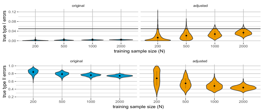
Refer to caption
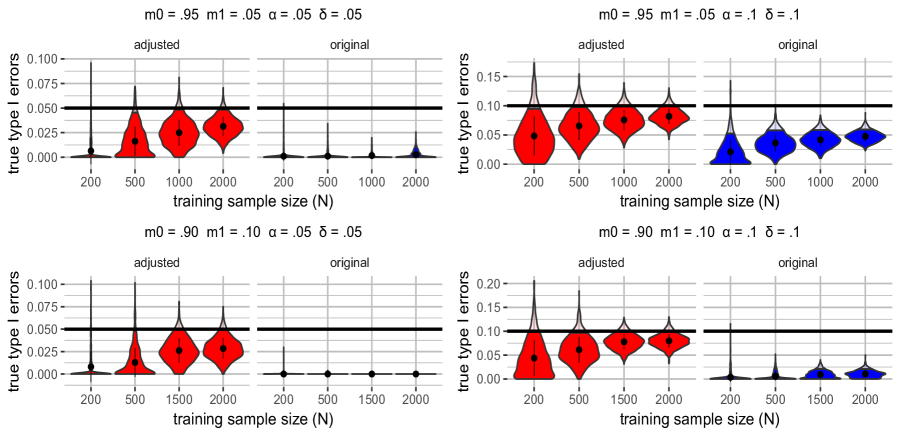
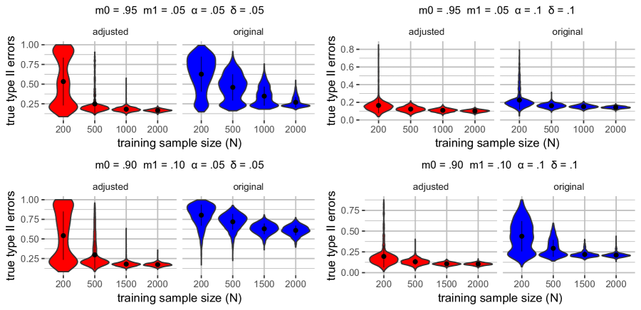
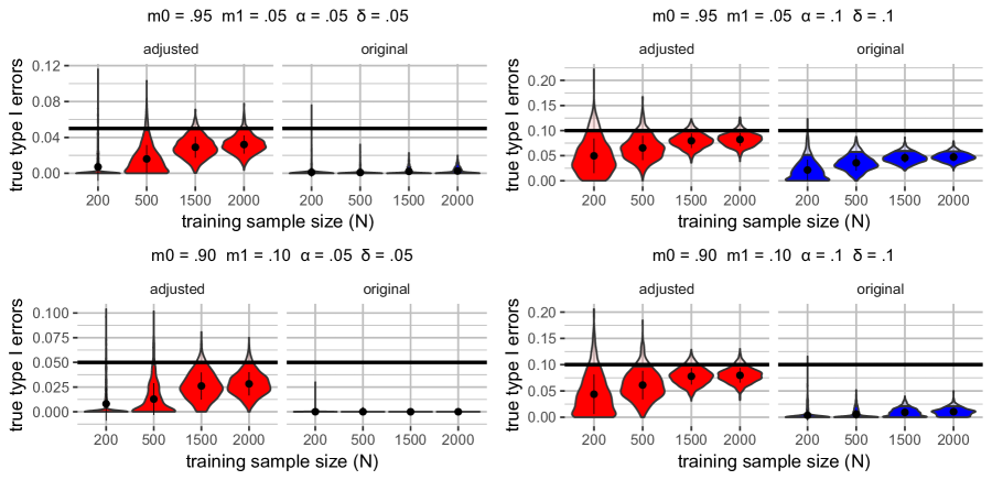
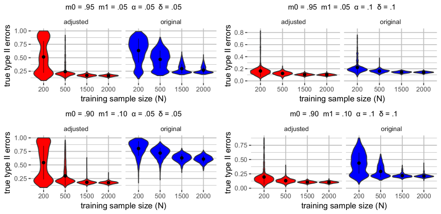
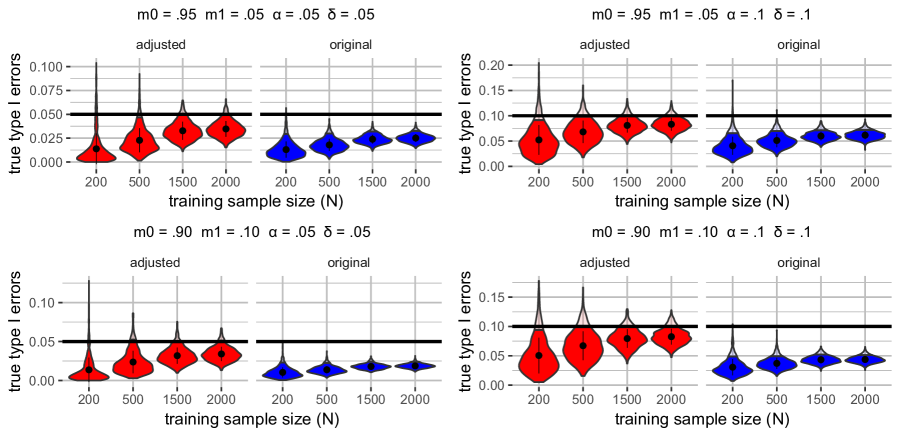
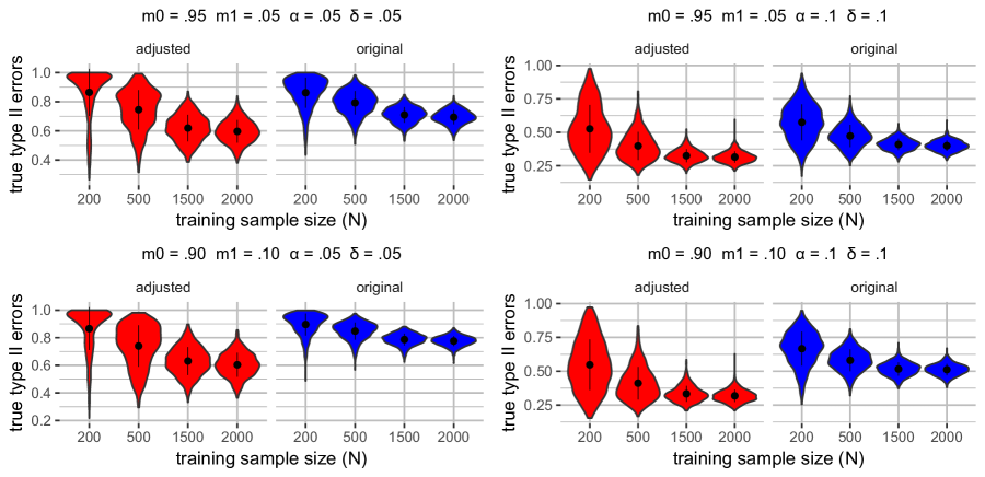
Figure 2: The original NP umbrella algorithm vs. a label-noise-adjusted version for Example 2. The plots in the left panel (blue) are the true type I and II errors for the original NP umbrella algorithm. The plots in the right panel (orange) are the true type I and II errors for the label-noise-adjusted NP umbrella algorithm with known corruption levels. The black dot and vertical bar in every violin represent mean and standard deviation, respectively. In the top row, the horizontal black line is α=0.05𝛼0.05\alpha=0.05 and the boundaries between lighter and darker color in each violin plot mark the 1δ=95%1𝛿percent951-\delta=95\% quantiles.
Example 2.

Let X0𝒩(0,1)similar-tosuperscript𝑋0𝒩01X^{0}\sim\mathcal{N}(0,1) and X1𝒩(2,1)similar-tosuperscript𝑋1𝒩21X^{1}\sim\mathcal{N}(2,1), m0=0.85subscript𝑚00.85m_{0}=0.85, m1=0.15subscript𝑚10.15m_{1}=0.15, α=0.05𝛼0.05\alpha=0.05 and δ=0.05𝛿0.05\delta=0.05. For simplicity, we use the identity scoring function: T^(X)=X^𝑇𝑋𝑋\hat{T}(X)=X. We generate N{200,500,1000,2000}𝑁20050010002000N\in\{200,500,1000,2000\} corrupted class 00 observations and train a classifier ϕ^k()subscript^italic-ϕsubscript𝑘\hat{\phi}_{k_{*}}(\cdot) based on them. Due to normality, we can analytically calculate the type I and II errors regarding the true labels. The above steps are repeated 1,00010001{,}000 times for every value of N𝑁N to graph the violin plots of both errors as shown in the left panel of Figure 2. Clearly, all the achieved true type I errors are much lower than the control target α𝛼\alpha and true type II errors are very high 666To make a contrast, we also plot in the right panel of Figure 2 the true type I and II errors of ϕ^k()subscript^italic-ϕsuperscript𝑘\hat{\phi}_{k^{*}}(\cdot), the classifier constructed by the label-noise-adjusted NP umbrella algorithm with known corruption levels to be introduced in the next section. The details to generate ϕ^k()subscript^italic-ϕsuperscript𝑘\hat{\phi}_{k^{*}}(\cdot)’s are skipped here, except we reveal that corrupted class 1 observations, in addition to the corrupted class 0 observations, are also needed to construct the thresholds..

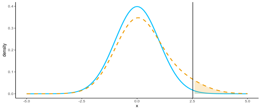
The phenomenon illustrated in the left panel of Figure 2 is not a contrived one. Indeed, under the class-conditional noise model (i.e., Assumption 1), at the same threshold level, the tail probability of corrupted class 00 is greater than that of true class 00 since the corrupted 00 distribution is a mixture of true 00 and 111 distributions. Figure 3 provides further illustration. In this figure, the black vertical line (x=2.52𝑥2.52x=2.52) marks the threshold of the classifier 1I{X>2.52}1I𝑋2.52{\rm 1}\kern-1.92004pt{\rm I}\{X>2.52\} whose corrupted type I error (i.e., the right tail probability under the orange dashed curve) is 0.050.050.05. In contrast, its true type I error (i.e., the right tail probability under the blue solid curve) is much smaller.
Refer to caption
Figure 3: The blue solid curve is the density of true class 00 (i.e., 𝒩(0,1)𝒩01\mathcal{N}(0,1)) and the orange dashed curve is the density of corrupted class 00 (i.e., a mixture of 𝒩(0,1)𝒩01\mathcal{N}(0,1) and 𝒩(2,1)𝒩21\mathcal{N}(2,1) with m0=0.85subscript𝑚00.85m_{0}=0.85). The black vertical line marks the threshold of the classifier 1I{X>2.52}1I𝑋2.52{\rm 1}\kern-1.92004pt{\rm I}\{X>2.52\} whose corrupted type I error is 0.050.050.05.

The above observation motivates us to create new label-noise-adjusted NP umbrella algorithms by carefully studying the discrepancy between true and corrupted type I errors, whose population-level relation is channeled by the class-conditional noise model and can be estimated based on data with corrupted labels alone. We will first develop a version for known corruption levels (i.e., Algorithm 1) and then a variant for unknown corruption levels (i.e., Algorithm 1#superscript1#1^{\#}). Although the latter variant is suitable for most applications, we believe that presenting first the known corruption level version streamlines the reasoning and presentation.

For methodology and theory development, we assume the following sampling scheme. Let 𝒮~0={X~j0}j=1N0superscript~𝒮0superscriptsubscriptsuperscriptsubscript~𝑋𝑗0𝑗1subscript𝑁0\tilde{\mathcal{S}}^{0}=\{\tilde{X}_{j}^{0}\}_{j=1}^{N_{0}} be corrupted class 00 observations and 𝒮~1={X~j1}j=1N1superscript~𝒮1superscriptsubscriptsubscriptsuperscript~𝑋1𝑗𝑗1subscript𝑁1\tilde{\mathcal{S}}^{1}=\{\tilde{X}^{1}_{j}\}_{j=1}^{N_{1}} corrupted class 111 ones. The sample sizes N0subscript𝑁0N_{0} and N1subscript𝑁1N_{1} are considered to be non-random numbers, and we assume that all observations in 𝒮~0superscript~𝒮0\tilde{\mathcal{S}}^{0} and 𝒮~1superscript~𝒮1\tilde{\mathcal{S}}^{1} are independent. Then, we divide 𝒮~0superscript~𝒮0\tilde{\mathcal{S}}^{0} into three random disjoint non-empty subsets. The first two parts 𝒮~b0subscriptsuperscript~𝒮0b\tilde{\mathcal{S}}^{0}_{\text{b}} and 𝒮~t0subscriptsuperscript~𝒮0t\tilde{\mathcal{S}}^{0}_{\text{t}} are used to train the base algorithm and determine the threshold candidates, respectively. The third part 𝒮~e0subscriptsuperscript~𝒮0e\tilde{\mathcal{S}}^{0}_{\text{e}} is used to estimate a correction term to account for the label noise. Similarly, we randomly divide 𝒮~1superscript~𝒮1\tilde{\mathcal{S}}^{1} into two disjoint non-empty subsets: 𝒮~b1subscriptsuperscript~𝒮1b\tilde{\mathcal{S}}^{1}_{\text{b}} and 𝒮~e1subscriptsuperscript~𝒮1e\tilde{\mathcal{S}}^{1}_{\text{e}}.

Let T^()^𝑇\hat{T}(\cdot) be a scoring function trained on 𝒮~b=𝒮~b0𝒮~b1subscript~𝒮bsuperscriptsubscript~𝒮b0subscriptsuperscript~𝒮1b\tilde{\mathcal{S}}_{\text{b}}=\tilde{\mathcal{S}}_{\text{b}}^{0}\cup\tilde{\mathcal{S}}^{1}_{\text{b}}. We apply T^()^𝑇\hat{T}(\cdot) to elements in 𝒮~t0subscriptsuperscript~𝒮0t\tilde{\mathcal{S}}^{0}_{\text{t}} and sort them in an increasing order: {t(1),,t(n)}subscript𝑡1subscript𝑡𝑛\{t_{(1)},\ldots,t_{(n)}\}, where n=|𝒮~t0|𝑛subscriptsuperscript~𝒮0tn=|\tilde{\mathcal{S}}^{0}_{\text{t}}|777In Appendix A, we summarize the notations related to the sampling scheme for the readers’ convenience.. These will serve as the threshold candidates, just as in the original NP umbrella algorithm. However, instead of ksubscript𝑘k_{*}, the label-noise-adjusted NP umbrella algorithm with known corruption levels will take the order ksuperscript𝑘k^{*} defined by

k=min{k{1,,n}:αk,δD^+(t(k))α},superscript𝑘:𝑘1𝑛subscript𝛼𝑘𝛿superscript^𝐷subscript𝑡𝑘𝛼k^{*}=\min\{k\in\{1,\ldots,n\}:\alpha_{k,\delta}-\hat{D}^{+}(t_{(k)})\leq\alpha\}\,,

where αk,δsubscript𝛼𝑘𝛿\alpha_{k,\delta}888The existence and uniqueness of αk,δsubscript𝛼𝑘𝛿\alpha_{k,\delta} are ensured by Lemma 5 in the Appendix. satisfies

j=kn(nj)αk,δnj(1αk,δ)j=δ,superscriptsubscript𝑗𝑘𝑛binomial𝑛𝑗superscriptsubscript𝛼𝑘𝛿𝑛𝑗superscript1subscript𝛼𝑘𝛿𝑗𝛿\displaystyle\sum_{j=k}^{n}{n\choose j}\alpha_{k,\delta}^{n-j}(1-\alpha_{k,\delta})^{j}=\delta\,, (3)

D^+()=D^()0:=max(D^(),0)superscript^𝐷^𝐷0assign^𝐷0\hat{D}^{+}(\cdot)=\hat{D}(\cdot)\vee 0:=\max(\hat{D}(\cdot),0) and D^()=1m0m0m1(F~^0T^()F~^1T^())^𝐷1subscript𝑚0subscript𝑚0subscript𝑚1superscriptsubscript^~𝐹0^𝑇superscriptsubscript^~𝐹1^𝑇\hat{D}(\cdot)=\frac{1-m_{0}}{m_{0}-m_{1}}\left(\hat{\tilde{F}}_{0}^{\hat{T}}(\cdot)-\hat{\tilde{F}}_{1}^{\hat{T}}(\cdot)\right), in which F~^0T^()superscriptsubscript^~𝐹0^𝑇\hat{\tilde{F}}_{0}^{\hat{T}}(\cdot) and F~^1T^()superscriptsubscript^~𝐹1^𝑇\hat{\tilde{F}}_{1}^{\hat{T}}(\cdot) are empirical estimates of F~0T^()superscriptsubscript~𝐹0^𝑇\tilde{F}_{0}^{\hat{T}}(\cdot) and F~1T^()superscriptsubscript~𝐹1^𝑇\tilde{F}_{1}^{\hat{T}}(\cdot) based on 𝒮~e0subscriptsuperscript~𝒮0e\tilde{\mathcal{S}}^{0}_{\text{e}} and 𝒮~e1subscriptsuperscript~𝒮1e\tilde{\mathcal{S}}^{1}_{\text{e}}, respectively.

1
Input : 𝒮~0superscript~𝒮0\tilde{\mathcal{S}}^{0}: sample of corrupted 00 observations
𝒮~1superscript~𝒮1\tilde{\mathcal{S}}^{1}: sample of corrupted 111 observations
α𝛼\alpha: type I error upper bound, 0<α<10𝛼10<\alpha<1
δ𝛿\delta: type I error violation rate target, 0<δ<10𝛿10<\delta<1
m0subscript𝑚0m_{0}: probability of a corrupted class 0 sample being of true class 0
m1subscript𝑚1m_{1}: probability of a corrupted class 1 sample being of true class 0
2
3𝒮~b0subscriptsuperscript~𝒮0b\tilde{\mathcal{S}}^{0}_{\text{b}}, 𝒮~t0subscriptsuperscript~𝒮0t\tilde{\mathcal{S}}^{0}_{\text{t}},𝒮~e0subscriptsuperscript~𝒮0eabsent\tilde{\mathcal{S}}^{0}_{\text{e}}\leftarrow random split on 𝒮~0superscript~𝒮0\tilde{\mathcal{S}}^{0}
4𝒮~b1subscriptsuperscript~𝒮1b\tilde{\mathcal{S}}^{1}_{\text{b}}, 𝒮~e1subscriptsuperscript~𝒮1eabsent\tilde{\mathcal{S}}^{1}_{\text{e}}\leftarrow random split on 𝒮~1superscript~𝒮1\tilde{\mathcal{S}}^{1}
𝒮~b𝒮~b1𝒮~b0subscript~𝒮bsubscriptsuperscript~𝒮1bsubscriptsuperscript~𝒮0b\tilde{\mathcal{S}}_{\text{b}}\leftarrow\tilde{\mathcal{S}}^{1}_{\text{b}}\cup\tilde{\mathcal{S}}^{0}_{\text{b}} ;
  // combine 𝒮~b0subscriptsuperscript~𝒮0b\tilde{\mathcal{S}}^{0}_{\text{b}} and 𝒮~b1subscriptsuperscript~𝒮1b\tilde{\mathcal{S}}^{1}_{\text{b}} as 𝒮~bsubscript~𝒮b\tilde{\mathcal{S}}_{\text{b}}
5
T^()^𝑇absent\hat{T}(\cdot)\leftarrow base classification algorithm(𝒮~b)subscript~𝒮b(\tilde{\mathcal{S}}_{\text{b}}) ;
  // train a scoring function on 𝒮~bsubscript~𝒮b\tilde{\mathcal{S}}_{\text{b}}
6
𝒯t={t1,t2,,tn}T^(𝒮~t0)subscript𝒯tsubscript𝑡1subscript𝑡2subscript𝑡𝑛^𝑇subscriptsuperscript~𝒮0t\mathcal{T}_{\text{t}}=\{t_{1},t_{2},\ldots,t_{n}\}\leftarrow\hat{T}(\tilde{\mathcal{S}}^{0}_{\text{t}}) ;
  // apply T^^𝑇\hat{T} to every entry in 𝒮~tsubscript~𝒮t\tilde{\mathcal{S}}_{\text{t}}
7
8{t(1),t(2),,t(n)}sort(𝒯t)subscript𝑡1subscript𝑡2subscript𝑡𝑛sortsubscript𝒯t\{t_{(1)},t_{(2)},\ldots,t_{(n)}\}\leftarrow\textsf{sort}(\mathcal{T}_{\text{t}})
9𝒯e0T^(𝒮~e0)subscriptsuperscript𝒯0e^𝑇subscriptsuperscript~𝒮0e\mathcal{T}^{0}_{\text{e}}\leftarrow\hat{T}(\tilde{\mathcal{S}}^{0}_{\text{e}})
𝒯e1T^(𝒮~e1)subscriptsuperscript𝒯1e^𝑇subscriptsuperscript~𝒮1e\mathcal{T}^{1}_{\text{e}}\leftarrow\hat{T}(\tilde{\mathcal{S}}^{1}_{\text{e}}) ;
  // apply T^^𝑇\hat{T} to all elements in 𝒮~e0subscriptsuperscript~𝒮0e\tilde{\mathcal{S}}^{0}_{\text{e}} and 𝒮~e1subscriptsuperscript~𝒮1e\tilde{\mathcal{S}}^{1}_{\text{e}}
10
11for k𝑘k in {1,,n}1𝑛\{1,\dots,n\} do
12      
      αk,δBinarySearch(δ,k,n)subscript𝛼𝑘𝛿BinarySearch𝛿𝑘𝑛\alpha_{k,\delta}\leftarrow\textsf{BinarySearch}(\delta,k,n) ;
        // compute αk,δsubscript𝛼𝑘𝛿\alpha_{k,\delta} through binary search
13      
14      F~^0T^(t(k))|𝒯e0|1t𝒯e01I{tt(k)}superscriptsubscript^~𝐹0^𝑇subscript𝑡𝑘superscriptsubscriptsuperscript𝒯0e1subscript𝑡subscriptsuperscript𝒯0e1I𝑡subscript𝑡𝑘\hat{\tilde{F}}_{0}^{\hat{T}}(t_{(k)})\leftarrow\left|\mathcal{T}^{0}_{\text{e}}\right|^{-1}\cdot\sum_{t\in\mathcal{T}^{0}_{\text{e}}}{\rm 1}\kern-1.92004pt{\rm I}\{t\leq t_{(k)}\}
      F~^1T^(t(k))|𝒯e1|1t𝒯e11I{tt(k)}superscriptsubscript^~𝐹1^𝑇subscript𝑡𝑘superscriptsubscriptsuperscript𝒯1e1subscript𝑡subscriptsuperscript𝒯1e1I𝑡subscript𝑡𝑘\hat{\tilde{F}}_{1}^{\hat{T}}(t_{(k)})\leftarrow\left|\mathcal{T}^{1}_{\text{e}}\right|^{-1}\cdot\sum_{t\in\mathcal{T}^{1}_{\text{e}}}{\rm 1}\kern-1.92004pt{\rm I}\{t\leq t_{(k)}\} ;
        // compute the empirical distributions
15      
      D^(t(k))1m0m0m1(F~^0T^(t(k))F~^1T^(t(k)))^𝐷subscript𝑡𝑘1subscript𝑚0subscript𝑚0subscript𝑚1superscriptsubscript^~𝐹0^𝑇subscript𝑡𝑘superscriptsubscript^~𝐹1^𝑇subscript𝑡𝑘\hat{D}(t_{(k)})\leftarrow\frac{1-m_{0}}{m_{0}-m_{1}}\left(\hat{\tilde{F}}_{0}^{\hat{T}}(t_{(k)})-\hat{\tilde{F}}_{1}^{\hat{T}}(t_{(k)})\right) ;
        // compute an estimate of R~0R0subscript~𝑅0subscript𝑅0\tilde{R}_{0}-R_{0}
16      
      D^+(t(k))D^(t(k))0superscript^𝐷subscript𝑡𝑘^𝐷subscript𝑡𝑘0\hat{D}^{+}(t_{(k)})\leftarrow\hat{D}(t_{(k)})\vee 0 ;
        // if D^(t(k))^𝐷subscript𝑡𝑘\hat{D}(t_{(k)}) is negative, then set it to 00
17      
18 end for
19
kmin{k{1,,n}:αk,δD^+(t(k))α}superscript𝑘:𝑘1𝑛subscript𝛼𝑘𝛿superscript^𝐷subscript𝑡𝑘𝛼k^{*}\leftarrow\min\{k\in\{1,\ldots,n\}:\alpha_{k,\delta}-\hat{D}^{+}(t_{(k)})\leq\alpha\} ;
  // select the order
20
ϕ^k()1I{T^()>t(k)}subscript^italic-ϕsuperscript𝑘1I^𝑇subscript𝑡superscript𝑘\hat{\phi}_{k^{*}}(\cdot)\leftarrow{\rm 1}\kern-1.92004pt{\rm I}\{\hat{T}(\cdot)>t_{(k^{*})}\} ;
  // construct an NP classifier
21
Output : ϕ^k()subscript^italic-ϕsuperscript𝑘\hat{\phi}_{k^{*}}(\cdot)
Algorithm 1 Label-noise-adjusted NP Umbrella Algorithm with known corruption levels

The entire construction process of ϕ^k()=1I{T^()>t(k)}subscript^italic-ϕsuperscript𝑘1I^𝑇subscript𝑡superscript𝑘\hat{\phi}_{k^{*}}(\cdot)={\rm 1}\kern-1.92004pt{\rm I}\{\hat{T}(\cdot)>t_{(k^{*})}\} is summarized and detailed in Algorithm 1. In this algorithm, to solve αk,δsubscript𝛼𝑘𝛿\alpha_{k,\delta}, we use a binary search subroutine (Algorithm 2 in Appendix B) on the function xj=kn(nk)xnj(1x)jmaps-to𝑥superscriptsubscript𝑗𝑘𝑛binomial𝑛𝑘superscript𝑥𝑛𝑗superscript1𝑥𝑗x\mapsto\sum_{j=k}^{n}{n\choose k}x^{n-j}(1-x)^{j}, leveraging its strict monotone decreasing property in x𝑥x. Interested readers are referred to the proof of Lemma 5 in the Appendix for further reasoning. Currently we randomly split 𝒮~0superscript~𝒮0\tilde{\mathcal{S}}^{0} and 𝒮~1superscript~𝒮1\tilde{\mathcal{S}}^{1} respectively into three and two equal sized subgroups. An optimal splitting strategy could be a subject for future research.

The key to the new algorithm is D^+()superscript^𝐷\hat{D}^{+}(\cdot), which adjusts for the label corruption. Indeed, the original NP umbrella algorithm can be seen as a special case of our approach where D^+()=0superscript^𝐷0\hat{D}^{+}(\cdot)=0. The numerical advantage of the new algorithm is demonstrated in the right panel of Figure 2 and in Section 5. We will prove in the next section that the label-noise-adjusted NP classifier ϕ^k()=1I{T^()>t(k)}subscript^italic-ϕsuperscript𝑘1I^𝑇subscript𝑡superscript𝑘\hat{\phi}_{k^{*}}(\cdot)={\rm 1}\kern-1.92004pt{\rm I}\{\hat{T}(\cdot)>t_{(k^{*})}\} controls true type I error with high probability while avoiding the excessive conservativeness of the original NP umbrella algorithm. Note that in contrast to the deterministic order ksubscript𝑘k_{*} in the original NP umbrella algorithm, the new order ksuperscript𝑘k^{*} is random, calling for much more involved technicalities to establish the theoretical properties of ϕ^k()subscript^italic-ϕsuperscript𝑘\hat{\phi}_{k^{*}}(\cdot).

3.3 Algorithm 1#superscript1#1^{\#}: label-noise-adjusted NP umbrella algorithm with unknown corruption levels

For most applications in practice, accurate corruption levels m0subscript𝑚0m_{0} and m1subscript𝑚1m_{1} are inaccessible. To address this, we propose Algorithm 1#superscript1#1^{\#}, a simple variant of Algorithm 1 that replaces m0subscript𝑚0m_{0} and m1subscript𝑚1m_{1} with estimates m0#superscriptsubscript𝑚0#m_{0}^{\#} and m1#superscriptsubscript𝑚1#m_{1}^{\#}. In all other respects the two algorithms are identical. Specifically, when estimating R~0R0subscript~𝑅0subscript𝑅0\tilde{R}_{0}-R_{0}, Algorithm 1#superscript1#1^{\#} uses D^#(t(k))=1m0#m0#m1#(F~^0T^(t(k))F~^1T^(t(k)))subscript^𝐷#subscript𝑡𝑘1superscriptsubscript𝑚0#superscriptsubscript𝑚0#superscriptsubscript𝑚1#superscriptsubscript^~𝐹0^𝑇subscript𝑡𝑘superscriptsubscript^~𝐹1^𝑇subscript𝑡𝑘\hat{D}_{\#}(t_{(k)})=\frac{1-m_{0}^{\#}}{m_{0}^{\#}-m_{1}^{\#}}\left(\hat{\tilde{F}}_{0}^{\hat{T}}(t_{(k)})-\hat{\tilde{F}}_{1}^{\hat{T}}(t_{(k)})\right) and D^#+(t(k))=D^#(t(k))0subscriptsuperscript^𝐷#subscript𝑡𝑘subscript^𝐷#subscript𝑡𝑘0\hat{D}^{+}_{\#}(t_{(k)})=\hat{D}_{\#}(t_{(k)})\vee 0. Then, Algorithm 1#superscript1#1^{\#} delivers the NP classifier ϕ^k#()=1I{T^()>t(k#)}subscript^italic-ϕsubscriptsuperscript𝑘#1I^𝑇subscript𝑡subscriptsuperscript𝑘#\hat{\phi}_{k^{*}_{\#}}(\cdot)={\rm 1}\kern-1.92004pt{\rm I}\{\hat{T}(\cdot)>t_{(k^{*}_{\#})}\}, where k#=min{k{1,,n}:αk,δD^#+(t(k))α}subscriptsuperscript𝑘#:𝑘1𝑛subscript𝛼𝑘𝛿subscriptsuperscript^𝐷#subscript𝑡𝑘𝛼k^{*}_{\#}=\min\{k\in\{1,\ldots,n\}:\alpha_{k,\delta}-\hat{D}^{+}_{\#}(t_{(k)})\leq\alpha\}. Due to the similarity with Algorithm 1, we do not re-produce the other steps of Algorithm 1#superscript1#1^{\#} to write it out in a full algorithm format.

Rather than supplying unbiased estimates for m0subscript𝑚0m_{0} and m1subscript𝑚1m_{1}, we will demonstrate that it is important that m0#superscriptsubscript𝑚0#m_{0}^{\#} and m1#superscriptsubscript𝑚1#m_{1}^{\#} are under-estimates of the corruption levels (i.e., m0#m0superscriptsubscript𝑚0#subscript𝑚0m_{0}^{\#}\geq m_{0} and m1#m1superscriptsubscript𝑚1#subscript𝑚1m_{1}^{\#}\leq m_{1} as in Assumption 1). In this work, we assume that domain experts supply these under-estimates. While it would be unrealistic to assume that these experts know m0subscript𝑚0m_{0} and m1subscript𝑚1m_{1} exactly, in many scenarios one can provide accurate bounds on these quantities. It would be interesting to investigate data-driven estimators that have such a property for future work.

4 Theory

In this section, we first elaborate the rationale behind Algorithm 1 (Section 4.1), and then show that under a few technical conditions, this new algorithm induces well-defined classifiers whose type I errors are bounded from above by the desired level with high probability (Section 4.2). Then we establish a similar result for its unknown-corruption-level variant, Algorithm 1#superscript1#1^{\#} (Section 4.3).

4.1 Rationale behind Algorithm 1

Proposition 1.

Let T^()^𝑇\hat{T}(\cdot) be a scoring function (e.g., sigmoid function in logistic regression) trained on 𝒮~bsubscript~𝒮b\tilde{\mathcal{S}}_{\emph{\text{b}}}. Applying T^()^𝑇\hat{T}(\cdot) to every element in 𝒮~t0subscriptsuperscript~𝒮0t\tilde{\mathcal{S}}^{0}_{\emph{\text{t}}}, we get a set of scores. Order these scores and denote them by {t(1),t(2),,t(n)}subscript𝑡1subscript𝑡2subscript𝑡𝑛\{t_{(1)},t_{(2)},\ldots,t_{(n)}\}, in which t(1)t(2)t(n)subscript𝑡1subscript𝑡2subscript𝑡𝑛t_{(1)}\leq t_{(2)}\leq\ldots\leq t_{(n)}. Then, for any α(0,1)𝛼01\alpha\in(0,1) and k{1,2,,n}𝑘12𝑛k\in\{1,2,\ldots,n\}, the classifier ϕ^k()=1I{T^()>t(k)}subscript^italic-ϕ𝑘1I^𝑇subscript𝑡𝑘\hat{\phi}_{k}(\cdot)={\rm 1}\kern-1.92004pt{\rm I}\{\hat{T}(\cdot)>t_{(k)}\} satisfies

IP(R~0(ϕ^k)>α)j=kn(nj)(1α)jα(nj),IPsubscript~𝑅0subscript^italic-ϕ𝑘𝛼superscriptsubscript𝑗𝑘𝑛binomial𝑛𝑗superscript1𝛼𝑗superscript𝛼𝑛𝑗{\rm I}\kern-1.43994pt{\rm P}\left(\tilde{R}_{0}(\hat{\phi}_{k})>{\alpha}\right)\leq\sum_{j=k}^{n}{n\choose j}(1-{\alpha})^{j}{\alpha}^{(n-j)}\,,

in which IPIP{\rm I}\kern-1.43994pt{\rm P} is regarding the randomness in all training observations, as well as additional randomness if we adopt certain random classification methods (e.g., random forest). Moreover, when T^()^𝑇\hat{T}(\cdot) is continuous almost surely, the above inequality obtains the equal sign.

Recall that R~0()subscript~𝑅0\tilde{R}_{0}(\cdot) denotes type I error regarding the corrupted labels. We omit a proof for Proposition 1 as it follows the same proof as its counterpart in Tong et al. (2018). For α,δ(0,1)𝛼𝛿01\alpha,\delta\in(0,1), recall that the original NP umbrella algorithm selects k=min{k{1,,n}:j=kn(nj)(1α)jα(nj)δ}subscript𝑘minconditional-set𝑘1𝑛superscriptsubscript𝑗𝑘𝑛binomial𝑛𝑗superscript1𝛼𝑗superscript𝛼𝑛𝑗𝛿k_{*}=\text{min}\{k\in\{1,\ldots,n\}:\sum_{j=k}^{n}{n\choose j}(1-{\alpha})^{j}{\alpha}^{(n-j)}\leq\delta\}. The smallest k𝑘k among all that satisfy j=kn(nj)(1α)jα(nj)δsuperscriptsubscript𝑗𝑘𝑛binomial𝑛𝑗superscript1𝛼𝑗superscript𝛼𝑛𝑗𝛿\sum_{j=k}^{n}{n\choose j}(1-{\alpha})^{j}{\alpha}^{(n-j)}\leq\delta is desirable because we also wish to minimize the type II error. There is a sample size requirement for this order statistics approach to work because a finite order ksubscript𝑘k_{*} should exist. Precisely, an order statistics approach works if the last order does; that is (1α)nδsuperscript1𝛼𝑛𝛿(1-\alpha)^{n}\leq\delta. This translates to Assumption 2 on n𝑛n, the sample size of 𝒮~t0subscriptsuperscript~𝒮0t\tilde{\mathcal{S}}^{0}_{\text{t}}. This is a mild requirement. For instance, when α=δ=0.05𝛼𝛿0.05\alpha=\delta=0.05, n𝑛n should be at least 595959.

Assumption 2.

nlogδ/log(1α)𝑛𝛿1𝛼n\geq\lceil\log\delta/\log(1-\alpha)\rceil, in which \lceil\cdot\rceil denotes the ceiling function.

In view of Proposition 1, the choice of ksubscript𝑘k_{*} guarantees IP(R~0(ϕ^k)α)1δIPsubscript~𝑅0subscript^italic-ϕsubscript𝑘𝛼1𝛿{\rm I}\kern-1.43994pt{\rm P}\left(\tilde{R}_{0}(\hat{\phi}_{k_{*}})\leq{\alpha}\right)\geq 1-\delta. In other words, if we were to ignore the label noise presence and apply the original NP umbrella algorithm, the type I error regarding the corrupted labels, R~0subscript~𝑅0\tilde{R}_{0}, is controlled under level α𝛼\alpha with probability at least 1δ1𝛿1-\delta. Moreover, the achieved R~0subscript~𝑅0\tilde{R}_{0} is usually not far from α𝛼\alpha when the sample size n𝑛n is much larger than the lower bound requirement. However, this is not our main target; what we really want is to control R0subscript𝑅0R_{0}. Example 2 in Section 3.1 convincingly demonstrates that in the presence of label noise, the achieved R0subscript𝑅0R_{0} after naive implementation of the original NP umbrella algorithm can be much lower than the control target α𝛼\alpha. This is no exception. To aid in analyzing the gap between R0subscript𝑅0R_{0} and R~0subscript~𝑅0\tilde{R}_{0}, we make the following assumption.

Assumption 3.

The scoring function T^^𝑇\hat{T} is trained such that F~0T^(z)>F~1T^(z)superscriptsubscript~𝐹0^𝑇𝑧superscriptsubscript~𝐹1^𝑇𝑧\tilde{F}_{0}^{\hat{T}}(z)>\tilde{F}_{1}^{\hat{T}}(z) for all zIR𝑧IRz\in{\rm I}\kern-1.43994pt{\rm R} with probability at least 1δ1(nb)1subscript𝛿1subscript𝑛b1-\delta_{1}(n_{\emph{b}}), where nb=|𝒮~b|subscript𝑛bsubscript~𝒮bn_{\emph{b}}=|\tilde{\mathcal{S}}_{\emph{b}}| and δ1(nb)subscript𝛿1subscript𝑛b\delta_{1}(n_{\emph{b}}) converges to 00 as nbsubscript𝑛bn_{\emph{b}} goes to infinity.

Loosely, Assumption 3 means that the scoring function trained on corrupted data still has the “correct direction.” For any classifier of the form ϕ^c()=1I{T^()>c}subscript^italic-ϕ𝑐1I^𝑇𝑐\hat{\phi}_{c}(\cdot)={\rm 1}\kern-1.92004pt{\rm I}\{\hat{T}(\cdot)>c\}, Assumption 3 implies that with probability at least 1δ1(nb)1subscript𝛿1subscript𝑛b1-\delta_{1}(n_{\text{b}}), P~0(ϕ^c(X)=0)>P~1(ϕ^c(X)=0)subscript~𝑃0subscript^italic-ϕ𝑐𝑋0subscript~𝑃1subscript^italic-ϕ𝑐𝑋0\tilde{P}_{0}(\hat{\phi}_{c}(X)=0)>\tilde{P}_{1}(\hat{\phi}_{c}(X)=0), which means that a corrupted class 00 observation is more likely to be classified as 00 than a corrupted class 111 observation is. Interested readers can find a concrete example that illustrates this mild assumption in the Appendix C (Example 3). Now we are ready to describe the discrepancy between R0subscript𝑅0R_{0} and R~0subscript~𝑅0\tilde{R}_{0}.

Lemma 1.

Let T^^𝑇\hat{T} be a scoring function trained on 𝒮~bsubscript~𝒮b\tilde{\mathcal{S}}_{\emph{\text{b}}} and ϕ^c()=1I{T^()>c}subscript^italic-ϕ𝑐1I^𝑇𝑐\hat{\phi}_{c}(\cdot)={\rm 1}\kern-1.92004pt{\rm I}\{\hat{T}(\cdot)>c\} be a classifier that thresholds the scoring function at cIR𝑐IRc\in{\rm I}\kern-1.43994pt{\rm R}. Denote D(c)=R~0(ϕ^c)R0(ϕ^c)𝐷𝑐subscript~𝑅0subscript^italic-ϕ𝑐subscript𝑅0subscript^italic-ϕ𝑐D(c)=\tilde{R}_{0}(\hat{\phi}_{c})-R_{0}(\hat{\phi}_{c}). Then, under Assumptions 1, 2 and 3, for given α𝛼\alpha and δ𝛿\delta, it holds that

IP(infcIRD(c)0)1δ1(nb) and  IP(R0(ϕ^k)>αD(t(k)))δ+δ1(nb),IPsubscriptinfimum𝑐IR𝐷𝑐01subscript𝛿1subscript𝑛b and  IPsubscript𝑅0subscript^italic-ϕsubscript𝑘𝛼𝐷subscript𝑡subscript𝑘𝛿subscript𝛿1subscript𝑛b\displaystyle{\rm I}\kern-1.43994pt{\rm P}\left(\inf_{c\in{\rm I}\kern-1.00795pt{\rm R}}D(c)\geq 0\right)\geq 1-\delta_{1}(n_{\emph{b}})\,\text{ }\text{and }\text{ }{\rm I}\kern-1.43994pt{\rm P}\left(R_{0}(\hat{\phi}_{k_{*}})>\alpha-D(t_{(k_{*})})\right)\leq\delta+\delta_{1}(n_{\emph{b}})\,,

where ksubscript𝑘k_{*} and δ𝛿\delta are related via equation (2). Moreover, we have

D(c)=M(F~0T^(c)F~1T^(c)),𝐷𝑐𝑀superscriptsubscript~𝐹0^𝑇𝑐superscriptsubscript~𝐹1^𝑇𝑐D(c)=M\left(\tilde{F}_{0}^{\hat{T}}(c)-\tilde{F}_{1}^{\hat{T}}(c)\right)\,, (4)

where M=(1m0)(m0m1)1𝑀1subscript𝑚0superscriptsubscript𝑚0subscript𝑚11M=(1-m_{0})(m_{0}-m_{1})^{-1}.

Note that D(c)𝐷𝑐D(c) measures the discrepancy between the corrupted type I error and the true type I error of the classifier ϕ^c()subscript^italic-ϕ𝑐\hat{\phi}_{c}(\cdot). Lemma 1 implies that with high probability, ϕ^k()subscript^italic-ϕsubscript𝑘\hat{\phi}_{k_{*}}(\cdot) has R0subscript𝑅0R_{0}, the type I error regarding true labels, under a level that is smaller than the target value α𝛼\alpha, and that the gap is measured by D(t(k))𝐷subscript𝑡subscript𝑘D(t_{(k_{*})}). It is important to note that D(c)𝐷𝑐D(c) is solely a function of the distributions of the corrupted data, and does not require any knowledge of the uncorrupted scores, so we are able to estimate this quantity from our observed data.

As argued previously, excessive conservativeness in type I error is not desirable because it is usually associated with a high type II error. Therefore, a new NP umbrella algorithm should adjust to the label noise, so that the resulting classifier respects the true type I error control target, but is not excessively conservative. Motivated by Lemma 1, our central plan is to choose some less conservative (i.e., smaller) order than that in the original NP umbrella algorithm, in view of the difference between R0subscript𝑅0R_{0} and R~0subscript~𝑅0\tilde{R}_{0}. Recall that δ(0,1)𝛿01\delta\in(0,1) is the target type I error violation rate. In the presence of label noise, we do not expect to control at this precise violation rate, but just some number around it.

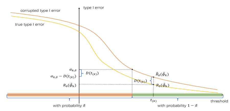
For any ϕ^k()subscript^italic-ϕ𝑘\hat{\phi}_{k}(\cdot), under Assumptions 1, 2 and 3, Lemma 1 implies R~0(ϕ^k)R0(ϕ^k)subscript~𝑅0subscript^italic-ϕ𝑘subscript𝑅0subscript^italic-ϕ𝑘\tilde{R}_{0}(\hat{\phi}_{k})\geq R_{0}(\hat{\phi}_{k}) with probability at least 1δ1(nb)1subscript𝛿1subscript𝑛b1-\delta_{1}(n_{\text{b}}). Note that the δ1(nb)subscript𝛿1subscript𝑛b\delta_{1}(n_{\text{b}}) term is small and asymptotically 00; we will ignore it in this section when motivating our new strategy. With this simplification, R~0(ϕ^k)subscript~𝑅0subscript^italic-ϕ𝑘\tilde{R}_{0}(\hat{\phi}_{k}) is always greater than R0(ϕ^k)subscript𝑅0subscript^italic-ϕ𝑘R_{0}(\hat{\phi}_{k}), as illustrated in Figure 4. The definition of αk,δsubscript𝛼𝑘𝛿\alpha_{k,\delta} in equation (3) and Proposition 1 imply with probability at least 1δ1𝛿1-\delta, αk,δR~0(ϕ^k)subscript𝛼𝑘𝛿subscript~𝑅0subscript^italic-ϕ𝑘\alpha_{k,\delta}\geq\tilde{R}_{0}(\hat{\phi}_{k}), which corresponds to the green region (the region on the right) in Figure 4. Since we only need 1δ1𝛿1-\delta probability control on R0subscript𝑅0R_{0}, it suffices to control R0subscript𝑅0R_{0} corresponding to this region. Combining the results αk,δR~0(ϕ^k)subscript𝛼𝑘𝛿subscript~𝑅0subscript^italic-ϕ𝑘\alpha_{k,\delta}\geq\tilde{R}_{0}(\hat{\phi}_{k}) and R~0(ϕ^k)R0(ϕ^k)subscript~𝑅0subscript^italic-ϕ𝑘subscript𝑅0subscript^italic-ϕ𝑘\tilde{R}_{0}(\hat{\phi}_{k})\geq R_{0}(\hat{\phi}_{k}), we have the inequalities αk,δαk,δD(t(k))R0(ϕ^k)subscript𝛼𝑘𝛿subscript𝛼𝑘𝛿𝐷subscript𝑡𝑘subscript𝑅0subscript^italic-ϕ𝑘\alpha_{k,\delta}\geq\alpha_{k,\delta}-D(t_{(k)})\geq R_{0}(\hat{\phi}_{k}) on our interested region (Recall D(t(k))=R~0(ϕ^k)R0(ϕ^k)𝐷subscript𝑡𝑘subscript~𝑅0subscript^italic-ϕ𝑘subscript𝑅0subscript^italic-ϕ𝑘D(t_{(k)})=\tilde{R}_{0}(\hat{\phi}_{k})-R_{0}(\hat{\phi}_{k})). By the previous argument, αk,δsubscript𝛼𝑘𝛿\alpha_{k,\delta} can be used as an upper bound for R0subscript𝑅0R_{0}, but to have a good type II error, a better choice is clearly the smaller αk,δD(t(k))subscript𝛼𝑘𝛿𝐷subscript𝑡𝑘\alpha_{k,\delta}-D(t_{(k)}). So if D(t(k))𝐷subscript𝑡𝑘D(t_{(k)}) were a known quantity, we can set the order to be k~=min{k{1,n}:αk,δD(t(k))α}superscript~𝑘:𝑘1𝑛subscript𝛼𝑘𝛿𝐷subscript𝑡𝑘𝛼\tilde{k}^{*}=\min\{k\in\{1\ldots,n\}:\alpha_{k,\delta}-D(t_{(k)})\leq\alpha\} and propose a classifier ϕ^k~()=1I{T^()>t(k~)}subscript^italic-ϕsuperscript~𝑘1I^𝑇subscript𝑡superscript~𝑘\hat{\phi}_{\tilde{k}^{*}}(\cdot)={\rm 1}\kern-1.92004pt{\rm I}\{\hat{T}(\cdot)>t_{(\tilde{k}^{*})}\}. This is to be compared with the order ksubscript𝑘k_{*} chosen by the original NP umbrella algorithm, which can be equivalently expressed as k=min{k{1,n}:αk,δα}subscript𝑘:𝑘1𝑛subscript𝛼𝑘𝛿𝛼k_{*}=\min\{k\in\{1\,\ldots,n\}:\alpha_{k,\delta}\leq\alpha\} (Lemma 5 in the Appendix). Then we have k~ksuperscript~𝑘subscript𝑘\tilde{k}^{*}\leq k_{*}, and so ϕ^k~()subscript^italic-ϕsuperscript~𝑘\hat{\phi}_{\tilde{k}^{*}}(\cdot) is less conservative than ϕ^k()subscript^italic-ϕsubscript𝑘\hat{\phi}_{k_{*}}(\cdot) in terms of type I error.

Refer to caption
Figure 4: A cartoon illustration of 1δ1𝛿1-\delta probability upper bound of type I error.

However, ϕ^k~()subscript^italic-ϕsuperscript~𝑘\hat{\phi}_{\tilde{k}^{*}}(\cdot) is not accessible because D𝐷D is unknown. Instead we estimate D𝐷D by replacing F~0T^subscriptsuperscript~𝐹^𝑇0\tilde{F}^{\hat{T}}_{0} and F~1T^superscriptsubscript~𝐹1^𝑇\tilde{F}_{1}^{\hat{T}} in (4) with their empirical distributions F~^0T^subscriptsuperscript^~𝐹^𝑇0\hat{\tilde{F}}^{\hat{T}}_{0} and F~^1T^subscriptsuperscript^~𝐹^𝑇1\hat{\tilde{F}}^{\hat{T}}_{1}, which are calculated using 𝒮~e0subscriptsuperscript~𝒮0e\tilde{\mathcal{S}}^{0}_{\text{e}} and 𝒮~e1subscriptsuperscript~𝒮1e\tilde{\mathcal{S}}^{1}_{\text{e}}, i.i.d. samples from the corrupted 00 and 111 observations. Note that these estimates are independent of 𝒮~bsubscript~𝒮b\tilde{\mathcal{S}}_{{\text{b}}} and 𝒮~t0subscriptsuperscript~𝒮0t\tilde{\mathcal{S}}^{0}_{{\text{t}}}. For a given T^^𝑇\hat{T}, we define for every cIR𝑐IRc\in{\rm I}\kern-1.43994pt{\rm R},

D^(c)=1m0m0m1(F~^0T^(c)F~^1T^(c)) and k=min{k{1,,n}:αk,δD^(t(k))αε},^𝐷𝑐1subscript𝑚0subscript𝑚0subscript𝑚1subscriptsuperscript^~𝐹^𝑇0𝑐subscriptsuperscript^~𝐹^𝑇1𝑐 and superscript𝑘absent:𝑘1𝑛subscript𝛼𝑘𝛿^𝐷subscript𝑡𝑘𝛼𝜀\displaystyle\hat{D}(c)=\frac{1-m_{0}}{m_{0}-m_{1}}\left(\hat{\tilde{F}}^{\hat{T}}_{0}(c)-\hat{\tilde{F}}^{\hat{T}}_{1}(c)\right)\,\text{ and }\,k^{**}=\min\{k\in\{1,\ldots,n\}:\alpha_{k,\delta}-\hat{D}(t_{(k)})\leq\alpha-\varepsilon\}\,,

in which a small ε>0𝜀0\varepsilon>0 is introduced to compensate for the randomness of D^^𝐷\hat{D} in the theory proofs. For simulation and real data, we actually just use ε=0𝜀0\varepsilon=0. Finally, the proposed new label-noise-adjusted NP classifier with known corruption levels is ϕ^k()=1I{T^()>t(k)}subscript^italic-ϕsuperscript𝑘1I^𝑇subscript𝑡superscript𝑘\hat{\phi}_{k^{*}}(\cdot)={\rm 1}\kern-1.92004pt{\rm I}\{\hat{T}(\cdot)>t_{(k^{*})}\}, in which ksuperscript𝑘k^{*} is a small twist from ksuperscript𝑘absentk^{**} by replacing D^^𝐷\hat{D} with its positive part. The construction of ϕ^k()subscript^italic-ϕsuperscript𝑘\hat{\phi}_{k^{*}}(\cdot) was detailed in Algorithm 1.

We have two comments on the implementation of Algorithm 1. First, though the ε𝜀\varepsilon compensation for the randomness is necessary for the theory proof, our empirical results suggest almost identical performance between ε=0𝜀0\varepsilon=0 relative to any small ε𝜀\varepsilon, so we recommend setting ε𝜀\varepsilon to 00 for simplicity, and we do not use the ε𝜀\varepsilon compensation in Algorithm 1. Second, in the order selection criterion of ksuperscript𝑘k^{*} in Algorithm 1, we use D^+=D^0:=max(D^,0)superscript^𝐷^𝐷0assign^𝐷0\hat{D}^{+}=\hat{D}\vee 0:=\max(\hat{D},0) instead of D^^𝐷\hat{D}, because empirically, although highly unlikely, D^^𝐷\hat{D} can be negative, which results in min{k{1,,n}:αk,δD^(t(k))α}min{k{1,,n}:αk,δα}:𝑘1𝑛subscript𝛼𝑘𝛿^𝐷subscript𝑡𝑘𝛼:𝑘1𝑛subscript𝛼𝑘𝛿𝛼\min\{k\in\{1,\ldots,n\}:\alpha_{k,\delta}-\hat{D}(t_{(k)})\leq\alpha\}\geq\min\{k\in\{1,\ldots,n\}:\alpha_{k,\delta}\leq\alpha\}. In this case, the new order could be greater than ksubscript𝑘k_{*}. Since we aim to reduce the conservativeness of the original NP umbrella algorithm, the possibility of kksuperscript𝑘subscript𝑘k^{*}\geq k_{*} will reverse this effort and worsen the conservativeness. To solve this issue, we force the empirical version of D𝐷D to be non-negative by replacing D^^𝐷\hat{D} with D^+superscript^𝐷\hat{D}^{+} in Algorithm 1.

4.2 Theoretical properties of Algorithm 1

In this subsection, we first formally establish that Algorithm 1 gives rise to valid classifiers (Lemma 2) and then show that these classifiers have the true type I errors controlled under α𝛼\alpha with high probability (Theorem 1).

Lemma 2.

Under Assumption 2, k=min{k{1,,n}:αk,δD^+(t(k))α}superscript𝑘:𝑘1𝑛subscript𝛼𝑘𝛿superscript^𝐷subscript𝑡𝑘𝛼k^{*}=\min\{k\in\{1,\ldots,n\}:\alpha_{k,\delta}-\hat{D}^{+}(t_{(k)})\leq\alpha\} in Algorithm 1 exists. Moreover, this label-noise-adjusted order is no larger than that chosen by the original NP umbrella algorithm; that is kksuperscript𝑘subscript𝑘k^{*}\leq k_{*}.

Lemma 2 implies that Algorithm 1 reduces the excessive conservativeness of the original NP umbrella algorithm on the type I error by choosing a smaller order statistic as the threshold. Moreover, if there is no label noise, i.e., when m0=1subscript𝑚01m_{0}=1 and m1=0subscript𝑚10m_{1}=0, we have k=min{k{1,,n}:αk,δα}=ksuperscript𝑘:𝑘1𝑛subscript𝛼𝑘𝛿𝛼subscript𝑘k^{*}=\min\{k\in\{1,\ldots,n\}:\alpha_{k,\delta}\leq\alpha\}=k_{*}. That is, Algorithm 1 reduces to the original NP umbrella algorithm.

Another important question is whether Algorithm 1 can control the true type I error with high probability. The following condition is assumed for the rest of this section.

Assumption 4.

The scoring function T^^𝑇\hat{T} is trained from a class of functions 𝒯𝒯\mathcal{T} such that the density functions for both T^(X~0)^𝑇superscript~𝑋0\hat{T}(\tilde{X}^{0}) and T^(X~1)^𝑇superscript~𝑋1\hat{T}(\tilde{X}^{1}) exist for every T^𝒯^𝑇𝒯\hat{T}\in\mathcal{T}. Then, we denote these two densities by f~0T^superscriptsubscript~𝑓0^𝑇\tilde{f}_{0}^{\hat{T}} and f~1T^superscriptsubscript~𝑓1^𝑇\tilde{f}_{1}^{\hat{T}}, respectively. Furthermore, supT^𝒯f~0T^f~1T^Csubscriptsupremum^𝑇𝒯subscriptnormsuperscriptsubscript~𝑓0^𝑇superscriptsubscript~𝑓1^𝑇𝐶\sup_{\hat{T}\in\mathcal{T}}\|\tilde{f}_{0}^{\hat{T}}\vee\tilde{f}_{1}^{\hat{T}}\|_{\infty}\leq C and infT^𝒯infz𝒟T^f~0T^(z)>csubscriptinfimum^𝑇𝒯subscriptinfimum𝑧subscript𝒟^𝑇subscriptsuperscript~𝑓^𝑇0𝑧𝑐\inf_{\hat{T}\in\mathcal{T}}\inf_{z\in\mathcal{D}_{\hat{T}}}\tilde{f}^{\hat{T}}_{0}(z)>c for some positive c𝑐c and C𝐶C with probability 1δ2(nb)1subscript𝛿2subscript𝑛b1-\delta_{2}(n_{\emph{b}}), where 𝒟T^subscript𝒟^𝑇\mathcal{D}_{\hat{T}} is the support of f~0T^subscriptsuperscript~𝑓^𝑇0\tilde{f}^{\hat{T}}_{0} and is a closed interval, and δ2(nb)subscript𝛿2subscript𝑛b\delta_{2}(n_{\emph{b}}) converges to 00 as nbsubscript𝑛bn_{\emph{b}} goes to infinity.

Note that Assumption 4 summarizes assumptions that we make for technical convenience in establishing the next theorem. In particular, we assume the existence of densities f~0T^superscriptsubscript~𝑓0^𝑇\tilde{f}_{0}^{\hat{T}} and f~1T^superscriptsubscript~𝑓1^𝑇\tilde{f}_{1}^{\hat{T}}, which holds if X~0superscript~𝑋0\tilde{X}^{0} and X~1superscript~𝑋1\tilde{X}^{1} have densities and T^()^𝑇\hat{T}(\cdot) is smooth. Moreover, we assume that with high probability, both the densities are uniformly bounded from above and f~0T^()subscriptsuperscript~𝑓^𝑇0\tilde{f}^{\hat{T}}_{0}(\cdot) is bounded uniformly from below.

Recall that in Algorithm 1, we set k=min{k{1,,n}:αk,δD^+(t(k))α}superscript𝑘:𝑘1𝑛subscript𝛼𝑘𝛿superscript^𝐷subscript𝑡superscript𝑘𝛼k^{*}=\min\{k\in\{1,\ldots,n\}:\alpha_{k,\delta}-\hat{D}^{+}(t_{(k^{*})})\leq\alpha\} without an ε𝜀\varepsilon term. Setting ε=0𝜀0\varepsilon=0 intuitively seems reasonable since, when the sample size is small, the sets {k{1,,n}:αk,δD^+(t(k))αε}conditional-set𝑘1𝑛subscript𝛼𝑘𝛿superscript^𝐷subscript𝑡superscript𝑘𝛼𝜀\{k\in\{1,\ldots,n\}:\alpha_{k,\delta}-\hat{D}^{+}(t_{(k^{*})})\leq\alpha-\varepsilon\} and {k{1,,n}:αk,δD^+(t(k))α}conditional-set𝑘1𝑛subscript𝛼𝑘𝛿superscript^𝐷subscript𝑡superscript𝑘𝛼\{k\in\{1,\ldots,n\}:\alpha_{k,\delta}-\hat{D}^{+}(t_{(k^{*})})\leq\alpha\} agree with high probability, and, when the sample size is large, concentration of random variables takes effect so there is little need for compensation for randomness. Our simulation results further reinforce this intuition. However, we include an ε𝜀\varepsilon term in the next theorem as this is required in our proof for the theory to hold.

Theorem 1.

Under Assumptions 1, 2, 3 and 4, the classifier ϕ^k()subscript^italic-ϕsuperscript𝑘\hat{\phi}_{k^{*}}(\cdot), given by Algorithm 1 with k=min{k{1,,n}:αk,δD^+(t(k))αε}superscript𝑘:𝑘1𝑛subscript𝛼𝑘𝛿superscript^𝐷subscript𝑡𝑘𝛼𝜀k^{*}=\min\{k\in\{1,\ldots,n\}:\alpha_{k,\delta}-\hat{D}^{+}(t_{(k)})\leq\alpha-\varepsilon\}, satisfies

IP(R0(ϕ^k)>α)δ+δ1(nb)+δ2(nb)+2e81nM2C2c2ε2+2e81ne0M2ε2+2e81ne1M2ε2,IPsubscript𝑅0subscript^italic-ϕsuperscript𝑘𝛼𝛿subscript𝛿1subscript𝑛bsubscript𝛿2subscript𝑛b2superscript𝑒superscript81𝑛superscript𝑀2superscript𝐶2superscript𝑐2superscript𝜀22superscript𝑒superscript81subscriptsuperscript𝑛0esuperscript𝑀2superscript𝜀22superscript𝑒superscript81subscriptsuperscript𝑛1esuperscript𝑀2superscript𝜀2\displaystyle{\rm I}\kern-1.43994pt{\rm P}\left(R_{0}(\hat{\phi}_{k^{*}})>\alpha\right)\leq\delta+\delta_{1}(n_{\emph{b}})+\delta_{2}(n_{\emph{b}})+2e^{-8^{-1}nM^{-2}C^{-2}c^{2}\varepsilon^{2}}+2e^{-8^{-1}n^{0}_{\emph{e}}M^{-2}\varepsilon^{2}}+2e^{-8^{-1}n^{1}_{\emph{e}}M^{-2}\varepsilon^{2}}\,,

in which nb=|𝒮~b|subscript𝑛bsubscript~𝒮bn_{\emph{\text{b}}}=|\tilde{\mathcal{S}}_{\emph{\text{b}}}|, n=|𝒮~t0|𝑛subscriptsuperscript~𝒮0tn=|\tilde{\mathcal{S}}^{0}_{\emph{\text{t}}}|, ne0=|𝒮~e0|subscriptsuperscript𝑛0esubscriptsuperscript~𝒮0en^{0}_{\emph{e}}=|\tilde{\mathcal{S}}^{0}_{\emph{\text{e}}}|, and ne1=|𝒮~e1|subscriptsuperscript𝑛1esubscriptsuperscript~𝒮1en^{1}_{\emph{e}}=|\tilde{\mathcal{S}}^{1}_{\emph{\text{e}}}|.

Note that the upper bound of IP(R0(ϕ^k)>α)IPsubscript𝑅0subscript^italic-ϕsuperscript𝑘𝛼{\rm I}\kern-1.43994pt{\rm P}\left(R_{0}(\hat{\phi}_{k^{*}})>\alpha\right) is δ𝛿\delta, our violation rate control target, plus a few terms which converge to zero as the sample sizes increase. To establish this inequality, we first exclude the complement of the events described in Assumption 3 and 4. Then, we further restrict ourselves on the event constructed by a Glivenko-Cantelli type inequality where D^^𝐷\hat{D} and D𝐷D only differ by 21εsuperscript21𝜀2^{-1}\varepsilon. There, the order selection criterion can be written as k=min{k{1,,n}:αk,δD(t(k))α21ε}superscript𝑘:𝑘1𝑛subscript𝛼𝑘𝛿𝐷subscript𝑡𝑘𝛼superscript21𝜀k^{*}=\min\{k\in\{1,\ldots,n\}:\alpha_{k,\delta}-D(t_{(k)})\leq\alpha-2^{-1}\varepsilon\}. The main difficulty of the proof is to handle the randomness of the threshold t(k)subscript𝑡superscript𝑘t_{(k^{*})}. Unlike the deterministic order ksubscript𝑘k_{*} in the original NP umbrella algorithm, the new order ksuperscript𝑘k^{*} is stochastic. As such, even when conditioning on T^^𝑇\hat{T}, t(k)subscript𝑡superscript𝑘t_{(k^{*})} is sill random and cannot be handled as a normal order statistic. Our solution is to find a high probability deterministic lower bound for t(k)subscript𝑡superscript𝑘t_{(k^{*})}. To do this, we introduce cksubscript𝑐𝑘c_{k}, the k/n𝑘𝑛k/n quantile of F~0T^subscriptsuperscript~𝐹^𝑇0\tilde{F}^{\hat{T}}_{0}, which is a deterministic value if we consider T^^𝑇\hat{T} to be fixed. Then, we show that D(t(k))𝐷subscript𝑡𝑘D(t_{(k)}) only differs from D(ck)𝐷subscript𝑐𝑘D(c_{k}) by 41εsuperscript41𝜀4^{-1}\varepsilon for all k𝑘k and that αk,δD(ck)α41εsubscript𝛼superscript𝑘𝛿𝐷subscript𝑐superscript𝑘𝛼superscript41𝜀\alpha_{k^{*},\delta}-D(c_{k^{*}})\leq\alpha-4^{-1}\varepsilon. Then, we define k0=min{k{1,,n}:αk,δD(ck)α41ε}subscript𝑘0:𝑘1𝑛subscript𝛼𝑘𝛿𝐷subscript𝑐𝑘𝛼superscript41𝜀k_{0}=\min\{k\in\{1,\ldots,n\}:\alpha_{k,\delta}-D(c_{k})\leq\alpha-4^{-1}\varepsilon\}, which is another deterministic value, given that T^^𝑇\hat{T} is considered to be fixed. Then, we find that k0ksubscript𝑘0superscript𝑘k_{0}\leq k^{*} and αk0,δD(t(k0))αsubscript𝛼subscript𝑘0𝛿𝐷subscript𝑡subscript𝑘0𝛼\alpha_{k_{0},\delta}-D(t_{(k_{0})})\leq\alpha with high probability. Therefore, t(k0)subscript𝑡subscript𝑘0t_{(k_{0})} is a high probability lower bound for t(k)subscript𝑡superscript𝑘t_{(k^{*})}. Moreover, t(k0)subscript𝑡subscript𝑘0t_{(k_{0})} is an order statistic with deterministic order (for fixed T^^𝑇\hat{T}) and thus its distribution can be written as a binomial probability. The fact αk0,δD(t(k0))αsubscript𝛼subscript𝑘0𝛿𝐷subscript𝑡subscript𝑘0𝛼\alpha_{k_{0},\delta}-D(t_{(k_{0})})\leq\alpha combined with Proposition 1 yields that the violation rate of ϕ^k0()subscript^italic-ϕsubscript𝑘0\hat{\phi}_{k_{0}}(\cdot) is smaller than δ𝛿\delta. The readers are referred to Appendix F for a complete proof.

4.3 Theoretical properties of Algorithm 1#superscript1#1^{\#}

In this subsection, we discuss the properties of Algorithm 1#superscript1#1^{\#}. Recall that m0#m0superscriptsubscript𝑚0#subscript𝑚0m_{0}^{\#}\geq m_{0} and m1#m1superscriptsubscript𝑚1#subscript𝑚1m_{1}^{\#}\leq m_{1} in Assumption 1 mean that the corruption levels are “underestimated.” As such, Algorithm 1#superscript1#1^{\#} produces a more conservative result than Algorithm 1. To see this, note that the only difference between two algorithms is that (1m0)(m0m1)11subscript𝑚0superscriptsubscript𝑚0subscript𝑚11(1-m_{0})(m_{0}-m_{1})^{-1} in Algorithm 1 is replaced with (1m0#)(m0#m1#)11superscriptsubscript𝑚0#superscriptsuperscriptsubscript𝑚0#superscriptsubscript𝑚1#1(1-m_{0}^{\#})(m_{0}^{\#}-m_{1}^{\#})^{-1} in Algorithm 1#superscript1#1^{\#}. The latter is no larger than the former, so we have a threshold in Algorithm 1#superscript1#1^{\#} larger than or equal to that in Algorithm 1.

On the other hand, under Assumption 1, Algorithm 1#superscript1#1^{\#} is still less conservative than the original NP umbrella algorithm. To digest this, we first consider the case where the label noise is totally “ignored”, i.e., m0#=1superscriptsubscript𝑚0#1m_{0}^{\#}=1 and m1#=0superscriptsubscript𝑚1#0m_{1}^{\#}=0. In this case, Algorithm 1#superscript1#1^{\#} is equivalent to the original NP umbrella algorithm. Then, since usually m0#<1superscriptsubscript𝑚0#1m_{0}^{\#}<1 and m1#>0superscriptsubscript𝑚1#0m_{1}^{\#}>0, Algorithm 1#superscript1#1^{\#} produces a smaller threshold than the NP original umbrella algorithm. Therefore, Algorithm 1#superscript1#1^{\#} overcomes, at least partially, the conservativeness issue of the original NP umbrella algorithm.

These insights are formalized in the following lemma.

Lemma 3.

Under Assumptions 1 - 2, k#=min{k{1,,n}:αk,δD^#+(t(k))α}subscriptsuperscript𝑘#:𝑘1𝑛subscript𝛼𝑘𝛿subscriptsuperscript^𝐷#subscript𝑡𝑘𝛼k^{*}_{\#}=\min\{k\in\{1,\ldots,n\}:\alpha_{k,\delta}-\hat{D}^{+}_{\#}(t_{(k)})\leq\alpha\} in Algorithm 1#superscript1#1^{\#} exists. Moreover, the order k#subscriptsuperscript𝑘#k^{*}_{\#} is between ksuperscript𝑘k^{*} and ksubscript𝑘k_{*}, i.e., kk#ksuperscript𝑘subscriptsuperscript𝑘#subscript𝑘k^{*}\leq k^{*}_{\#}\leq k_{*}.

Next we establish a high probability control on type I error for Algorithm 1#superscript1#1^{\#}. Recall that a high probability control on type I error for Algorithm 1 was established in Theorem 1. In view of Lemma 3, ϕ^k#()subscript^italic-ϕsubscriptsuperscript𝑘#\hat{\phi}_{k^{*}_{\#}}(\cdot) produced in Algorithm 1#superscript1#1^{\#} has a larger threshold, and thus smaller true type I error, than that of ϕ^k()subscript^italic-ϕsuperscript𝑘\hat{\phi}_{k^{*}}(\cdot) produced by Algorithm 1. Then, a high probability control on true type I error of ϕ^k#()subscript^italic-ϕsubscriptsuperscript𝑘#\hat{\phi}_{k^{*}_{\#}}(\cdot) naturally follows. This result is summarized in the following corollary.

Corollary 1.

Under Assumptions 1 - 4, the classifier ϕ^k#()subscript^italic-ϕsubscriptsuperscript𝑘#\hat{\phi}_{k^{*}_{\#}}(\cdot) given by Algorithm 1#superscript1#1^{\#} with k#=min{k{1,,n}:αk,δD^#+(t(k))αε}subscriptsuperscript𝑘#:𝑘1𝑛subscript𝛼𝑘𝛿subscriptsuperscript^𝐷#subscript𝑡𝑘𝛼𝜀k^{*}_{\#}=\min\{k\in\{1,\ldots,n\}:\alpha_{k,\delta}-\hat{D}^{+}_{\#}(t_{(k)})\leq\alpha-\varepsilon\}, satisfies

IP(R0(ϕ^k#)>α)δ+δ1(nb)+δ2(nb)+2e81nM2C2c2ε2+2e81ne0M2ε2+2e81ne1M2ε2.IPsubscript𝑅0subscript^italic-ϕsubscriptsuperscript𝑘#𝛼𝛿subscript𝛿1subscript𝑛bsubscript𝛿2subscript𝑛b2superscript𝑒superscript81𝑛superscript𝑀2superscript𝐶2superscript𝑐2superscript𝜀22superscript𝑒superscript81subscriptsuperscript𝑛0esuperscript𝑀2superscript𝜀22superscript𝑒superscript81subscriptsuperscript𝑛1esuperscript𝑀2superscript𝜀2\displaystyle{\rm I}\kern-1.43994pt{\rm P}\left(R_{0}(\hat{\phi}_{k^{*}_{\#}})>\alpha\right)\leq\delta+\delta_{1}(n_{\emph{b}})+\delta_{2}(n_{\emph{b}})+2e^{-8^{-1}nM^{-2}C^{-2}c^{2}\varepsilon^{2}}+2e^{-8^{-1}n^{0}_{\emph{e}}M^{-2}\varepsilon^{2}}+2e^{-8^{-1}n^{1}_{\emph{e}}M^{-2}\varepsilon^{2}}\,.

in which nb=|𝒮~b|subscript𝑛bsubscript~𝒮bn_{\emph{\text{b}}}=|\tilde{\mathcal{S}}_{\emph{\text{b}}}|, n=|𝒮~t0|𝑛subscriptsuperscript~𝒮0tn=|\tilde{\mathcal{S}}^{0}_{\emph{\text{t}}}|, ne0=|𝒮~e0|subscriptsuperscript𝑛0esubscriptsuperscript~𝒮0en^{0}_{\emph{e}}=|\tilde{\mathcal{S}}^{0}_{\emph{\text{e}}}|, and ne1=|𝒮~e1|subscriptsuperscript𝑛1esubscriptsuperscript~𝒮1en^{1}_{\emph{e}}=|\tilde{\mathcal{S}}^{1}_{\emph{\text{e}}}|.

5 Numerical Analysis

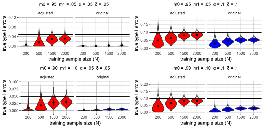
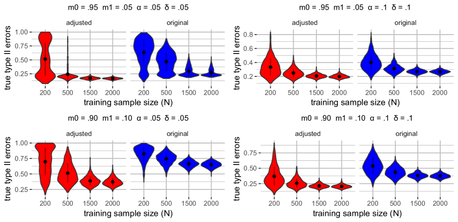
In this section, we apply Algorithms 1 (known corruption levels) and 1#superscript1#1^{\#} (unknown corruption levels) on simulated and real datasets, and compare with other methods in the literature. We present the (approximate) type I error violation rates999Strictly speaking, the observed type I error violation rate is only an approximation to the real violation rate. The approximation is two-fold: i). in each repetition of an experiment, the population type I error is approximated by empirical type I error on a large test set; ii). the violation rate should be calculated based on infinite repetitions of the experiment, but we only calculate it based on a finite number of repetitions. However, such approximation is unavoidable in numerical studies. and the averages of (approximate) true type II errors. Besides the simulations in this section, we have additional simulations in Appendix D.1. Furthermore, the violin plots associated with selected simulation are presented in Appendix D.3.

As a justification of the minor discrepancy between our theory and implementation, readers can find in Appendix D.5 the results for a slightly different implementation of Algorithm 1, in which k=min{k{1,,n}:αk,δD^+(t(k))αε}superscript𝑘:𝑘1𝑛subscript𝛼𝑘𝛿superscript^𝐷subscript𝑡𝑘𝛼𝜀k^{*}=\min\{k\in\{1,\ldots,n\}:\alpha_{k,\delta}-\hat{D}^{+}(t_{(k)})\leq\alpha-\varepsilon\} and ε=0.0001𝜀0.0001\varepsilon=0.0001. In principle, it is possible that setting ε>0𝜀0\varepsilon>0 will make ksuperscript𝑘k^{*} larger than when ε=0𝜀0\varepsilon=0 as {k{1,2,,n},αk,δD^+(t(k))αk,δε}formulae-sequence𝑘12𝑛subscript𝛼𝑘𝛿superscript^𝐷subscript𝑡𝑘subscript𝛼𝑘𝛿𝜀\{k\in\{1,2,\ldots,n\},\alpha_{k,\delta}-\hat{D}^{+}(t_{(k)})\leq\alpha_{k,\delta}-\varepsilon\} is a subset of {k{1,2,,n},αk,δD^+(t(k))αk,δ}formulae-sequence𝑘12𝑛subscript𝛼𝑘𝛿superscript^𝐷subscript𝑡𝑘subscript𝛼𝑘𝛿\{k\in\{1,2,\ldots,n\},\alpha_{k,\delta}-\hat{D}^{+}(t_{(k)})\leq\alpha_{k,\delta}\}. This will make the threshold larger and the type I error and the violation rate smaller. However, since ε=0.0001𝜀0.0001\varepsilon=0.0001 is a very small value, its effect on ksuperscript𝑘k^{*} is very minor. In numerical studies, two implementations (ε=0.0001𝜀0.0001\varepsilon=0.0001 in the Appendix vs. ε=0𝜀0\varepsilon=0 in this section) give nearly identical results for all examples. Both implementations generate the same type I errors and type II errors for most (at least 95%percent9595\%) cases. Moreover, the difference in violation rates of the two implementations is no larger than a very small number 0.1δ0.1𝛿0.1\delta.

5.1 Simulation

5.1.1 Algorithm 1.

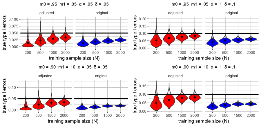
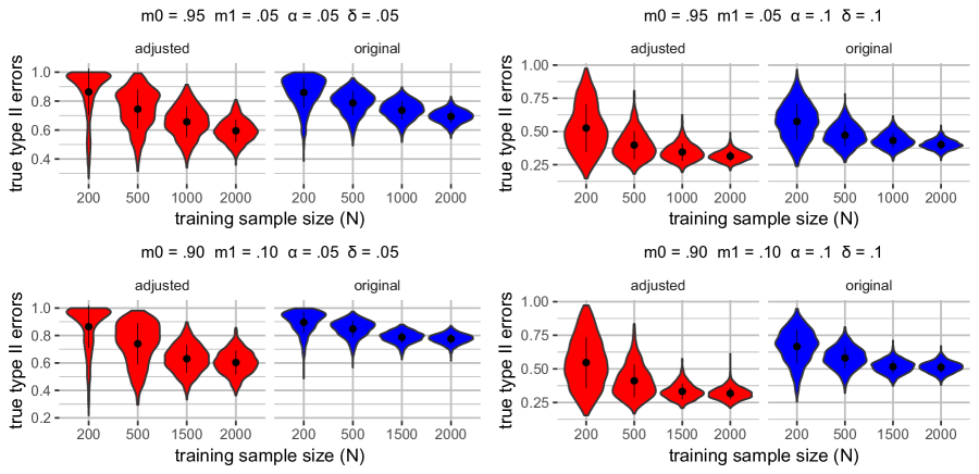
We present three distributional settings for Algorithm 1 (known m0subscript𝑚0m_{0} and m1subscript𝑚1m_{1}). In each setting, 2N2𝑁2N observations are generated as a training sample, of which half are from the corrupted class 00 and half from the corrupted class 111. The number N𝑁N varies from 200200200 to 2,00020002{,}000. To approximate the true type I and II errors, we generate 20,0002000020{,}000 true class 00 observations and 20,0002000020{,}000 true class 111 observations as the evaluation set. For each distribution and sample size combination, we repeat the procedure 1,00010001{,}000 times. Algorithm 1 (“adjusted”) and the original NP umbrella algorithm (“original”) are both applied, paired with different base algorithms.

Simulation 1 (Gaussian Distribution).

Let X0𝒩(μ0,Σ)similar-tosuperscript𝑋0𝒩subscript𝜇0ΣX^{0}\sim\mathcal{N}(\mu_{0},\Sigma) and X1𝒩(μ1,Σ)similar-tosuperscript𝑋1𝒩subscript𝜇1ΣX^{1}\sim\mathcal{N}(\mu_{1},\Sigma), where μ0=(0,0,0),μ1=(1,1,1)formulae-sequencesubscript𝜇0superscript000topsubscript𝜇1superscript111top\mu_{0}=(0,0,0)^{\top},\mu_{1}=(1,1,1)^{\top} and

Σ=(210121012),Σmatrix210121012\displaystyle\Sigma=\begin{pmatrix}2&-1&0\\ -1&2&-1\\ 0&-1&2\end{pmatrix}\,,

and the base algorithm is linear discriminant analysis (LDA). For different (m0,m1,α,δ)subscript𝑚0subscript𝑚1𝛼𝛿(m_{0},m_{1},\alpha,\delta) combinations, the (approximate) type I error violation rates and the averages of (approximate) true type II errors generated by Algorithm 1 are reported in Tables 1 and 2, respectively.

Table 1: (Approximate) type I error violation rates over 1,00010001{,}000 repetitions for Simulation 1. Standard errors (×103absentsuperscript103\times 10^{-3}) in parentheses.
N𝑁N
m0=.95,m1=.05formulae-sequencesubscript𝑚0.95subscript𝑚1.05m_{0}=.95,m_{1}=.05
α=.05,δ=.05formulae-sequence𝛼.05𝛿.05\alpha=.05,\delta=.05
m0=.9,m1=.1formulae-sequencesubscript𝑚0.9subscript𝑚1.1m_{0}=.9,m_{1}=.1
α=.05,δ=.05formulae-sequence𝛼.05𝛿.05\alpha=.05,\delta=.05
m0=.95,m1=.05formulae-sequencesubscript𝑚0.95subscript𝑚1.05m_{0}=.95,m_{1}=.05
α=.1,δ=.1formulae-sequence𝛼.1𝛿.1\alpha=.1,\delta=.1
m0=.9,m1=.1formulae-sequencesubscript𝑚0.9subscript𝑚1.1m_{0}=.9,m_{1}=.1
α=.1,δ=.1formulae-sequence𝛼.1𝛿.1\alpha=.1,\delta=.1
adjusted original adjusted original adjusted original adjusted original
200200200 .026.026.026 (5.03)5.03(5.03) .001.001.001 (1.00)1.00(1.00) .033.033.033 (5.65)5.65(5.65) 00 (0)0(0) .078.078.078 (8.84)8.84(8.84) .003.003.003 (1.73)1.73(1.73) .073.073.073 (8.23)8.23(8.23) 00 (0)0(0)
500500500 .031.031.031 (5.40)5.40(5.40) 00 (0)0(0) .046.046.046 (6.63)6.63(6.63) 00 (0)0(0) .090.090.090 (9.05)9.05(9.05) .001.001.001 (1.00)1.00(1.00) .085.085.085 (8.82)8.82(8.82) 00 (0)0(0)
1,00010001{,}000 .038.038.038 (5.97)5.97(5.97) 00 (0)0(0) .049.049.049 (6.83)6.83(6.83) 00 (0)0(0) .105.105.105 (9.70)9.70(9.70) 00 (0)0(0) .081.081.081 (8.63)8.63(8.63) 00 (0)0(0)
2,00020002{,}000 .053.053.053 (6.96)6.96(6.96) 00 (0)0(0) .046.046.046 (6.63)6.63(6.63) 00 (0)0(0) .087.087.087 (8.92)8.92(8.92) 00 (0)0(0) .099.099.099 (9.45)9.45(9.45) 00 (0)0(0)
Table 2: Averages of (approximate) true type II errors over 1,00010001{,}000 repetitions for Simulation 1. Standard errors (×103absentsuperscript103\times 10^{-3}) in parentheses.
N𝑁N
m0=.95,m1=.05formulae-sequencesubscript𝑚0.95subscript𝑚1.05m_{0}=.95,m_{1}=.05
α=.05,δ=.05formulae-sequence𝛼.05𝛿.05\alpha=.05,\delta=.05
m0=.9,m1=.1formulae-sequencesubscript𝑚0.9subscript𝑚1.1m_{0}=.9,m_{1}=.1
α=.05,δ=.05formulae-sequence𝛼.05𝛿.05\alpha=.05,\delta=.05
m0=.95,m1=.05formulae-sequencesubscript𝑚0.95subscript𝑚1.05m_{0}=.95,m_{1}=.05
α=.1,δ=.1formulae-sequence𝛼.1𝛿.1\alpha=.1,\delta=.1
m0=.9,m1=.1formulae-sequencesubscript𝑚0.9subscript𝑚1.1m_{0}=.9,m_{1}=.1
α=.1,δ=.1formulae-sequence𝛼.1𝛿.1\alpha=.1,\delta=.1
adjusted original adjusted original adjusted original adjusted original
200200200 .685.685.685 (7.16)7.16(7.16) .706.706.706 (4.65)4.65(4.65) .697.697.697 (7.06)7.06(7.06) .826.826.826 (3.54)3.54(3.54) .333.333.333 (3.93)3.93(3.93) .403.403.403 (3.56)3.56(3.56) .369.369.369 (4.93)4.93(4.93) .537.537.537 (4.03)4.03(4.03)
500500500 .481.481.481 (4.08)4.08(4.08) .590.590.590 (2.99)2.99(2.99) .512.512.512 (4.92)4.92(4.92) .743.743.743 (2.79)2.79(2.79) .249.249.249 (1.94)1.94(1.94) .307.307.307 (1.83)1.83(1.83) .257.257.257 (2.21)2.21(2.21) .436.436.436 (2.48)2.48(2.48)
1,00010001{,}000 .396.396.396 (2.53)2.53(2.53) .534.534.534 (2.19)2.19(2.19) .387.387.387 (2.37)2.37(2.37) .663.663.663 (1.68)1.68(1.68) .218.218.218 (1.18)1.18(1.18) .287.287.287 (1.22)1.22(1.22) .213.213.213 (1.01)1.01(1.01) .381.381.381 (1.28)1.28(1.28)
2,00020002{,}000 .350.350.350 (1.51)1.51(1.51) .491.491.491 (1.45)1.45(1.45) .371.371.371 (1.99)1.99(1.99) .651.651.651 (1.45)1.45(1.45) .201.201.201 (.76).76(.76) .268.268.268 (.77).77(.77) .205.205.205 (.87).87(.87) .375.375.375 (1.01)1.01(1.01)
Simulation 2 (Uniform Distribution within Circles).

Let X0superscript𝑋0X^{0} and X1superscript𝑋1X^{1} be uniformly distributed within unit circles respectively centered at (0,0)superscript00top(0,0)^{\top} and (1,1)superscript11top(1,1)^{\top}. The base algorithm is logistic regression. We only report (approximate) type I error violation rates and the averages of (approximate) true type II errors generated by Algorithm 1 for one combination (m0=.95subscript𝑚0.95m_{0}=.95, m1=.05subscript𝑚1.05m_{1}=.05, α=.1𝛼.1\alpha=.1 and δ=.1𝛿.1\delta=.1) in Table 3.

Table 3: (Approximate) type I error violation rates, and averages of (approximate) true type II errors over 1,00010001{,}000 repetitions for Simulation 2 (m0=.95subscript𝑚0.95m_{0}=.95, m1=.05subscript𝑚1.05m_{1}=.05, α=.1𝛼.1\alpha=.1 and δ=.1𝛿.1\delta=.1). Standard errors (×103absentsuperscript103\times 10^{-3}) in parentheses.
N𝑁N
(approximate)
violation rate
averages of
(approximate) true
type II errors
adjusted original adjusted original
200200200 .079.079.079 (8.53)8.53(8.53) .006.006.006 (2.44)2.44(2.44) .164.164.164 (2.77)2.77(2.77) .226.226.226 (3.35)3.35(3.35)
500500500 .086.086.086 (8.87)8.87(8.87) .001.001.001 (1.00)1.00(1.00) .123.123.123 (.92).92(.92) .161.161.161 (.80).80(.80)
1,00010001{,}000 .085.085.085 (8.82)8.82(8.82) 00 (0)0(0) .109.109.109 (.61).61(.61) .151.151.151 (.58).58(.58)
2,00020002{,}000 .085.085.085 (8.82)8.82(8.82) 00 (0)0(0) .101.101.101 (.44).44(.44) .142.142.142 (.39).39(.39)
Simulation 3 (T Distribution).

Let X0superscript𝑋0X^{0} and X1superscript𝑋1X^{1} be t-distributed with shape matrix ΣΣ\Sigma, which was specified in Simulation 1, 444 degrees of freedom, and centered at (0,0,0)superscript000top(0,0,0)^{\top} and (1,1,1)superscript111top(1,1,1)^{\top} respectively. The base algorithm is LDA. Similar to the previous simulation, we only report (approximate) type I error violation rates and the averages of (approximate) true type II errors generated by Algorithm 1 for one combination (m0=.95subscript𝑚0.95m_{0}=.95, m1=.05subscript𝑚1.05m_{1}=.05, α=.1𝛼.1\alpha=.1 and δ=.1𝛿.1\delta=.1) in Table 4.

Table 4: (Approximate) type I error violation rates, and averages of (approximate) true type II errors over 1,00010001{,}000 repetitions for Simulation 3 (m0=.95subscript𝑚0.95m_{0}=.95, m1=.05subscript𝑚1.05m_{1}=.05, α=.1𝛼.1\alpha=.1 and δ=.1𝛿.1\delta=.1). Standard errors (×103absentsuperscript103\times 10^{-3}) in parentheses.
N𝑁N
(approximate)
violation rate
average of
(approximate) true
type II errors
adjusted original adjusted original
200200200 .068.068.068 (7.96)7.96(7.96) .008.008.008 (2.82)2.82(2.82) .526.526.526 (5.67)5.67(5.67) .575.575.575 (4.32)4.32(4.32)
500500500 .085.085.085 (8.82)8.82(8.82) .002.002.002 (1.41)1.41(1.41) .398.398.398 (3.32)3.32(3.32) .472.472.472 (2.59)2.59(2.59)
1,00010001{,}000 .090.090.090 (9.05)9.05(9.05) 00 (0)0(0) .345.345.345 (2.07)2.07(2.07) .432.432.432 (1.78)1.78(1.78)
2,00020002{,}000 .093.093.093 (9.19)9.19(9.19) 00 (0)0(0) .314.314.314 (1.24)1.24(1.24) .401.401.401 (1.18)1.18(1.18)

The results from Simulations 1-3 confirm that the original NP umbrella algorithm is overly conservative on type I error when there is label noise in the training data, resulting in type I error violation rates (close to) 0 in all settings. In contrast, the label-noise-adjusted Algorithm 1 has type I errors controlled at the specified level with high probability and achieves much better type II errors.

5.1.2 Algorithm 1#superscript1#1^{\#}.

In this section, we show numerically that under the NP paradigm, the “under-estimates” of corruption levels serve Algorithm 1#superscript1#1^{\#} well, while ”over-estimates” do not.

Simulation 4.

The distributional setting is the same as in Simulation 1. Different combinations of m0#superscriptsubscript𝑚0#m_{0}^{\#} and m1#superscriptsubscript𝑚1#m_{1}^{\#} are used. the (approximate) type I error violation rates and the averages of (approximate) true type II errors generated by Algorithm 1#superscript1#1^{\#} for one combination (m0=.95subscript𝑚0.95m_{0}=.95, m1=.05subscript𝑚1.05m_{1}=.05, α=.1𝛼.1\alpha=.1 and δ=.1𝛿.1\delta=.1) are reported in Tables 5 and 6.

Table 5: (Approximate) type I error violation rates over 1,00010001{,}000 repetitions for Simulation 4. Standard errors (×103absentsuperscript103\times 10^{-3}) in parentheses.
N𝑁N
m0#=.93,superscriptsubscript𝑚0#.93m_{0}^{\#}=.93,
m1#=.07superscriptsubscript𝑚1#.07m_{1}^{\#}=.07
m0#=.95,superscriptsubscript𝑚0#.95m_{0}^{\#}=.95,
m1#=.05superscriptsubscript𝑚1#.05m_{1}^{\#}=.05
m0#=.97,superscriptsubscript𝑚0#.97m_{0}^{\#}=.97,
m1#=.03superscriptsubscript𝑚1#.03m_{1}^{\#}=.03
original
200200200 .136(10.85).13610.85.136(10.85) .078(8.48).0788.48.078(8.48) .055(7.21).0557.21.055(7.21) .003(1.73).0031.73.003(1.73)
500500500 .218(13.06).21813.06.218(13.06) .090(9.05).0909.05.090(9.05) .038(6.05).0386.05.038(6.05) .001(1.00).0011.00.001(1.00)
1,00010001,000 .324(14.81).32414.81.324(14.81) .105(9.70).1059.70.105(9.70) .012(3.44).0123.44.012(3.44) 0(0)000(0)
2,00020002,000 .462(15.77).46215.77.462(15.77) .087(8.92).0878.92.087(8.92) .005(2.23).0052.23.005(2.23) 0(0)000(0)
Table 6: (Approximate) type II error violation rates over 1,00010001{,}000 repetitions for Simulation 4. Standard errors (×103absentsuperscript103\times 10^{-3}) in parentheses.
N𝑁N
m0#=.93,superscriptsubscript𝑚0#.93m_{0}^{\#}=.93,
m1#=.07superscriptsubscript𝑚1#.07m_{1}^{\#}=.07
m0#=.95,superscriptsubscript𝑚0#.95m_{0}^{\#}=.95,
m1#=.05superscriptsubscript𝑚1#.05m_{1}^{\#}=.05
m0#=.97,superscriptsubscript𝑚0#.97m_{0}^{\#}=.97,
m1#=.03superscriptsubscript𝑚1#.03m_{1}^{\#}=.03
original
200200200 .287(3.43).2873.43.287(3.43) .333(3.92).3333.92.333(3.92) .373(4.62).3734.62.373(4.62) .403(3.56).4033.56.403(3.56)
500500500 .215(1.61).2151.61.215(1.61) .249(1.94).2491.94.249(1.94) .285(2.22).2852.22.285(2.22) .307(1.83).3071.83.307(1.83)
1,00010001,000 .189(1.02).1891.02.189(1.02) .218(1.18).2181.18.218(1.18) .250(1.37).2501.37.250(1.37) .287(1.22).2871.22.287(1.22)
2,00020002,000 .174(.65).174.65.174(.65) .201(.76).201.76.201(.76) .230(.86).230.86.230(.86) .268(.77).268.77.268(.77)

The second to the last column in Table 5 confirms that, using strict under-estimates of corruption levels (i.e., m0#>m0superscriptsubscript𝑚0#subscript𝑚0m_{0}^{\#}>m_{0} and m1#<m1superscriptsubscript𝑚1#subscript𝑚1m_{1}^{\#}<m_{1}), the type I error control objective is satisfied. Note that we also include the strict over-estimate scenarios in the second column (i.e., m0#<m0superscriptsubscript𝑚0#subscript𝑚0m_{0}^{\#}<m_{0} and m1#>m1superscriptsubscript𝑚1#subscript𝑚1m_{1}^{\#}>m_{1}), where we see that the type I violation rates exceed the target δ𝛿\delta. Hence the under-estimate requirement in the theory part is not merely for technical convenience. Table 6 confirms that the using strict under-estimates would lead to higher type II errors than using the true corruption levels. This is a necessary price to pay for not knowing the exact levels, but still it is better than totally ignoring the label corruption and applying the original NP umbrella algorithm.

We state again that in this work, we rely on domain experts to supply under-estimates of corruption levels. In the literature, there are existing estimators. For example, we implement estimators proposed by Liu and Tao (2016) in Simulations 6 and 7 in Appendix D.1. There, we would see that those estimators do not help Algorithm 1#superscript1#1^{\#} achieve the type I error control objective. But this is not a problem with these estimators themselves. Even “oracle” consistent and unbiased estimators that center at m0subscript𝑚0m_{0} and m1subscript𝑚1m_{1} do not serve the purpose either, as revealed in Simulation 8 in Appendix D.1. As expected, given our discussion about the need for under-estimates of the corruption levels (i.e., m0#m0superscriptsubscript𝑚0#subscript𝑚0m_{0}^{\#}\geq m_{0} and m1#m1superscriptsubscript𝑚1#subscript𝑚1m_{1}^{\#}\leq m_{1}), Algorithm 1#superscript1#1^{\#} performs poorly using these unbiased estimates. It could be an interesting topic for future research to identify an efficient method for producing biased estimates which will satisfy (with high probability) the bounds necessary to ensure correct type 1 error control.

5.1.3 Benchmark Algorithms.

In the next simulation, we apply existing state-of-the-art algorithms that perform classification on data with label noise. In particular, we apply the backward loss correction algorithm in Patrini et al. (2017) and the T-revision method in Xia et al. (2019). Since we focus on the NP paradigm, we will report the same (approximate) type I error violation rates and averages of (approximate) true type II errors as for our own methods.

Simulation 5.

The distributional setting is the same as in Simulation 1. The (approximate) type I error violation rates and averages of (approximate) true type II errors generated by benchmark algorithms for one combination (m0=.95subscript𝑚0.95m_{0}=.95, m1=.05subscript𝑚1.05m_{1}=.05, α=.1𝛼.1\alpha=.1 and δ=.1𝛿.1\delta=.1) are reported in Table 7 in the main and Table 16 in Appendix D.4, respectively.

Table 7: (Approximate) type I error violation rates over 1,00010001{,}000 repetitions for Simulation 5 (m0=.95subscript𝑚0.95m_{0}=.95, m1=.05subscript𝑚1.05m_{1}=.05, α=.1𝛼.1\alpha=.1 and δ=.1𝛿.1\delta=.1). Standard errors (×103absentsuperscript103\times 10^{-3}) in parentheses.
algorithms N𝑁N
200200200 500500500 1,00010001{,}000 2,00020002{,}000
T-revision .713(14.31).71314.31.713(14.31) .675(14.82).67514.82.675(14.82) .651(15.08).65115.08.651(15.08) .621(15.35).62115.35.621(15.35)
backward loss correction
(known corruption levels)
.994(2.44).9942.44.994(2.44) .977(4.74).9774.74.977(4.74) .770(13.31).77013.31.770(13.31) .127(10.53).12710.53.127(10.53)
backward loss correction
(unknown corruption levels)
.984(3.97).9843.97.984(3.97) .793(5.20).7935.20.793(5.20) .320(6.89).3206.89.320(6.89) .131(3.60).1313.60.131(3.60)

In Simulation 5, the benchmark algorithms fail to control the true type I error with the pre-specified high probability. This is understandable, as none of the benchmark algorithms have α𝛼\alpha or δ𝛿\delta as inputs. As such, these algorithms, unlike Algorithms 1 or 1#superscript1#1^{\#}, are not designed for the NP paradigm.

5.2 Real Data Analysis

We analyze a canonical email spam dataset (Hopkins et al., 1999), which consists of 4,60146014{,}601 observations including 575757 attributes describing characteristics of emails and a 01010-1 class label. Here, 111 represents spam email while 00 represents non-spam, and the type I/II error is defined accordingly. The labels in the dataset are all assumed to be correct.

We create corrupted labels according to the class-conditional noise model. Concretely, we flip the labels of true class 00 observations with probability r0subscript𝑟0r_{0} and flip the labels of true class 111 observations with probability r1subscript𝑟1r_{1}. Note that m0subscript𝑚0m_{0} and m1subscript𝑚1m_{1} are IP(Y=0Y~=0)IP𝑌conditional0~𝑌0{\rm I}\kern-1.43994pt{\rm P}(Y=0\mid\tilde{Y}=0) and IP(Y=0Y~=1)IP𝑌conditional0~𝑌1{\rm I}\kern-1.43994pt{\rm P}(Y=0\mid\tilde{Y}=1), respectively, while r0=IP(Y~=1Y=0)subscript𝑟0IP~𝑌conditional1𝑌0r_{0}={\rm I}\kern-1.43994pt{\rm P}(\tilde{Y}=1\mid Y=0) and r1=IP(Y~=0Y=1)subscript𝑟1IP~𝑌conditional0𝑌1r_{1}={\rm I}\kern-1.43994pt{\rm P}(\tilde{Y}=0\mid Y=1). In our analysis, we choose m0=0.95subscript𝑚00.95m_{0}=0.95 and m1=0.05subscript𝑚10.05m_{1}=0.05, which implies setting r0=0.032subscript𝑟00.032r_{0}=0.032 and r1=0.078subscript𝑟10.078r_{1}=0.078 101010This is an application of the Bayes theorem with IP(Y=0)IP𝑌0{\rm I}\kern-1.79993pt{\rm P}(Y=0) estimated to be 0.6100.6100.610, which is the proportion of class 00 observations in the whole dataset.. For each training and evaluation procedure, we split the data by stratified sampling into training and evaluation sets. Specifically, 20%percent2020\% of the true class 00 observations and 20%percent2020\% of the true class 111 observations are randomly selected to form the training dataset, and the rest of the observations form the evaluation dataset. In total, the training set contains 921921921 observations and the evaluation set contains 3,68036803{,}680 observations. The larger evaluation set is reserved to better approximate (population-level) true type I/II error. We leave the evaluation data untouched, but randomly flip the training data label according to the calculated r0subscript𝑟0r_{0} and r1subscript𝑟1r_{1}. Four base algorithms are coupled with the original and new NP umbrella algorithms, with α=δ=0.1𝛼𝛿0.1\alpha=\delta=0.1. We repeat the procedure 1,00010001{,}000 times.

The (approximate) type I error violation rates and averages of (approximate) true type II errors generated by Algorithm 1 and the original NP umbrella algorithm are summarized in Table 8. Similar to the simulation studies, we observe that Algorithm 1 correctly controls type I error at the right level, while the original NP umbrella algorithm is significantly overly conservative on type I error, and consequently has much higher type II error. We also summarize the results generated by Algorithm 1#superscript1#1^{\#} in Tables 9 and 10. Clearly, while strict under-estimates lead to higher type II errors than using exact corruption levels, the type I error control objective is achieved, and the type II error is better than just ignoring label corruption and applying the original NP umbrella algorithm.

Table 8: (Approximate) type I error violation rates, and averages of (approximate) true type II errors by Algorithm 1 and original NP umbrella algorithm over 1,00010001{,}000 repetitions for the email spam data. Standard errors (×103absentsuperscript103\times 10^{-3}) in parentheses.
(approximate)
violation rate
average of
(approximate) true
type II errors
adjusted original adjusted original
penalized logistic regression .082(8.68).0828.68.082(8.68) 0(0)000(0) .205(2.65).2052.65.205(2.65) .272(2.71).2722.71.272(2.71)
linear discriminant analysis .096(9.32).0969.32.096(9.32) 0(0)000(0) .226(3.05).2263.05.226(3.05) .314(2.77).3142.77.314(2.77)
support vector machine .093(9.19).0939.19.093(9.19) .004(2.00).0042.00.004(2.00) .183(3.15).1833.15.183(3.15) .218(1.93).2181.93.218(1.93)
random forests .080(8.58).0808.58.080(8.58) 0(0)000(0) .120(1.13).1201.13.120(1.13) .152(1.54).1521.54.152(1.54)
Table 9: (Approximate) type I error violation rates by Algorithm 1#superscript1#1^{\#} over 1,00010001{,}000 repetitions for the email spam data. Standard errors (×103absentsuperscript103\times 10^{-3}) in parentheses.
m0#=0.93,subscriptsuperscript𝑚#00.93m^{\#}_{0}=0.93,
m1#=0.07subscriptsuperscript𝑚#10.07m^{\#}_{1}=0.07
m0#=0.95,subscriptsuperscript𝑚#00.95m^{\#}_{0}=0.95,
m1#=0.05subscriptsuperscript𝑚#10.05m^{\#}_{1}=0.05
m0#=0.97,subscriptsuperscript𝑚#00.97m^{\#}_{0}=0.97,
m1#=0.03subscriptsuperscript𝑚#10.03m^{\#}_{1}=0.03
original
penalized logistic regression .231(13.33).23113.33.231(13.33) .082(8.68).0828.68.082(8.68) .028(5.22).0285.22.028(5.22) 0(0)000(0)
linear discriminant analysis .223(13.17).22313.17.223(13.17) .096(9.32).0969.32.096(9.32) .023(4.74).0234.74.023(4.74) 0(0)000(0)
support vector machine .220(13.11).22013.11.220(13.11) .093(9.19).0939.19.093(9.19) .026(5.03).0265.03.026(5.03) .004(2.00).0042.00.004(2.00)
random forest .238(13.47).23813.47.238(13.47) .080(8.58).0808.58.080(8.58) .019(4.32).0194.32.019(4.32) 0(0)000(0)
Table 10: Averages of (approximate) true type II errors by Algorithm 1#superscript1#1^{\#} over 1,00010001{,}000 repetitions for the email spam data. Standard errors (×103absentsuperscript103\times 10^{-3}) in parentheses.
m0#=0.93,subscriptsuperscript𝑚#00.93m^{\#}_{0}=0.93,
m1#=0.07subscriptsuperscript𝑚#10.07m^{\#}_{1}=0.07
m0#=0.95,subscriptsuperscript𝑚#00.95m^{\#}_{0}=0.95,
m1#=0.05subscriptsuperscript𝑚#10.05m^{\#}_{1}=0.05
m0#=0.97,subscriptsuperscript𝑚#00.97m^{\#}_{0}=0.97,
m1#=0.03subscriptsuperscript𝑚#10.03m^{\#}_{1}=0.03
original
penalized logistic regression .165(2.04).1652.04.165(2.04) .205(2.65).2052.65.205(2.65) .254(3.10).2543.10.254(3.10) .272(2.71).2722.71.272(2.71)
linear discriminant analysis .213(2.54).2132.54.213(2.54) .226(3.05).2263.05.226(3.05) .314(3.37).3143.37.314(3.37) .314(2.77).3142.77.314(2.77)
support vector machine .138(1.20).1381.20.138(1.20) .183(3.15).1833.15.183(3.15) .199(2.11).1992.11.199(2.11) .218(1.93).2181.93.218(1.93)
random forest .102(.78).102.78.102(.78) .120(1.13).1201.13.120(1.13) .143(1.41).1431.41.143(1.41) .152(1.54).1521.54.152(1.54)

To make a comparison, we also apply the loss correction algorithm in Patrini et al. (2017) and the T-revision method in Xia et al. (2019) to the email spam data, with results summarized in Table 17 in Appendix D.4. Since these benchmark algorithms are not designed for the NP paradigm, as discussed in Section 5.1, none of the (approximate) true type I error violation rates are controlled as we desire. In addition to the email spam data, we also apply Algorithm 1 to the CIFAR10 dataset (Krizhevsky et al., 2009) and successfully have the type I error controlled (Appendix D.2).

6 Discussion

Under the NP paradigm, we developed the first label-noise-adjusted umbrella algorithms. There are several interesting directions for future research. First, we can consider a more complex noise model in which the corruption levels depend on both the class and features. Another direction is to consider data-driven “under-estimates” of the corruption levels in the class-conditional noise model and develop (distributional) model-specific adjustment algorithms. For instance, we can adopt the linear discriminant analysis model, i.e., X0𝒩(μ0,Σ)similar-tosuperscript𝑋0𝒩subscript𝜇0ΣX^{0}\sim\mathcal{N}(\mu_{0},\Sigma) and X1𝒩(μ1,Σ)similar-tosuperscript𝑋1𝒩subscript𝜇1ΣX^{1}\sim\mathcal{N}(\mu_{1},\Sigma).

7 Acknowledgements

We would like to Dr. Xiao Han from the University of Science and Technology of China and Dr. Min Zhou from United International College for inspirational discussions. This work was partially supported by U.S. NSF grant DMS 2113500.

REFERENCES

  • (1)
  • Blanchard et al. (2016) Blanchard, G., Flaska, M., Handy, G., Pozzi, S., and Scott, C. (2016), “Classification with asymmetric label noise: Consistency and maximal denoising,” Electronic Journal of Statistics, 10(2), 2780–2824.
  • Brazdil and Konolige (1990) Brazdil, P., and Konolige, K. (1990), “Machine Learning, Meta-Reasoning and Logics,” Springer, .
  • Brodley and Friedl (1999a) Brodley, C. E., and Friedl, M. A. (1999a), “Identifying mislabeled training data,” Journal of Artificial Intelligence Research, 11, 131–167.
  • Brodley and Friedl (1999b) Brodley, C., and Friedl, M. (1999b), “Identifying mislabeled training data,” Journal of Artificial Intelligence Research, 11, 131–167.
  • Cannings et al. (2020) Cannings, T. I., Fan, Y., and Samworth, R. J. (2020), “Classification with imperfect training labels,” Biometrika, 107(2), 311–330.
  • Cannon et al. (2002) Cannon, A., Howse, J., Hush, D., and Scovel, C. (2002), “Learning with the Neyman-Pearson and min-max criteria,” Los Alamos National Laboratory, Tech. Rep. LA-UR, pp. 02–2951.
  • Cao et al. (2012) Cao, J., Kwong, S., and Wang, R. (2012), “A noise-detection based AdaBoost algorithm for mislabeled data,” Pattern Recognition, 45(12), 4451–4465.
  • Ghosh et al. (2015) Ghosh, A., Manwani, N., and Sastry, P. (2015), “Making risk minimization tolerant to label noise,” Neurocomputing, 160, 93–107.
  • Guyon et al. (1996) Guyon, I., Matic, N., Vapnik, V. et al. (1996), “Discovering Informative Patterns and Data Cleaning.,”.
  • Hickey (1996) Hickey, R. J. (1996), “Noise modelling and evaluating learning from examples,” Artificial Intelligence, 82(1-2), 157–179.
  • Hopkins et al. (1999) Hopkins, M., Reeber, E., Forman, G., and Suermondt, J. (1999), “Spambase data set,” Hewlett-Packard Labs, 1(7).
  • Khardon and Wachman (2007) Khardon, R., and Wachman, G. (2007), “Noise tolerant variants of the perceptron algorithm,” Journal of Machine Learning Research, 8(Feb), 227–248.
  • Krizhevsky et al. (2009) Krizhevsky, A., Hinton, G. et al. (2009), “Learning multiple layers of features from tiny images,” , .
  • Lachenbruch (1966) Lachenbruch, P. A. (1966), “Discriminant analysis when the initial samples are misclassified,” Technometrics, 8(4), 657–662.
  • Lachenbruch (1979) Lachenbruch, P. A. (1979), “Note on initial misclassification effects on the quadratic discriminant function,” Technometrics, 21(1), 129–132.
  • Liu and Tao (2016) Liu, T., and Tao, D. (2016), “Classification with noisy labels by importance reweighting,” IEEE Transactions on Pattern Analysis and Machine Intelligence, 38(3), 447–461.
  • MacDonald (2011) MacDonald, O. (2011), “Physician Perspectives on Preventing Diagnostic Errors,” https://www.kff.org/wp-content/uploads/sites/2/2013/05/quantiamd_preventingdiagnosticerrors_whitepaper_1.pdf, .
  • Manwani and Sastry (2013) Manwani, N., and Sastry, P. (2013), “Noise tolerance under risk minimization,” IEEE Transactions on Cybernetics, 43(3), 1146–1151.
  • Natarajan et al. (2013) Natarajan, N., Dhillon, I. S., Ravikumar, P. K., and Tewari, A. (2013), Learning with noisy labels,, in Advances in Neural Information Processing Systems, pp. 1196–1204.
  • Okamoto and Yugami (1997) Okamoto, S., and Yugami, N. (1997), An average-case analysis of the k-nearest neighbor classifier for noisy domains,, in IJCAI (1), pp. 238–245.
  • Orr (1998) Orr, K. (1998), “Data quality and systems theory,” Communications of the ACM, 41(2), 66–71.
  • Patrini et al. (2017) Patrini, G., Rozza, A., Krishna Menon, A., Nock, R., and Qu, L. (2017), Making deep neural networks robust to label noise: A loss correction approach,, in Proceedings of the IEEE Conference on Computer Vision and Pattern Recognition, pp. 1944–1952.
  • Redman (1998) Redman, T. (1998), “The impact of poor data quality on the typical enterprise,” Communications of the ACM, 2(2), 79–82.
  • Rigollet and Tong (2011) Rigollet, P., and Tong, X. (2011), “Neyman-pearson classification, convexity and stochastic constraints,” Journal of Machine Learning Research, 12(Oct), 2831–2855.
  • Scott and Nowak (2005) Scott, C., and Nowak, R. (2005), “A Neyman-Pearson approach to statistical learning,” IEEE Transactions on Information Theory, 51(11), 3806–3819.
  • Sukhbaatar and Fergus (2014) Sukhbaatar, S., and Fergus, R. (2014), “Learning from noisy labels with deep neural networks,” arXiv preprint arXiv:1406.2080, 2(3), 4.
  • Tong (2013) Tong, X. (2013), “A plug-in approach to Neyman-Pearson classification,” Journal of Machine Learning Research, 14(1), 3011–3040.
  • Tong et al. (2018) Tong, X., Feng, Y., and Li, J. J. (2018), “Neyman-Pearson classification algorithms and NP receiver operating characteristics,” Science Advances, 4(2), eaao1659.
  • Tong et al. (2020) Tong, X., Xia, L., Wang, J., and Feng, Y. (2020), “Neyman-Pearson classification: parametrics and sample size requirement,” Journal of Machine Learning Research, 21, 1–18.
  • Xia et al. (2019) Xia, X., Liu, T., Wang, N., Han, B., Gong, C., Niu, G., and Sugiyama, M. (2019), “Are anchor points really indispensable in label-noise learning?,” Advances in Neural Information Processing Systems, 32, 6838–6849.
  • Zhao et al. (2016) Zhao, A., Feng, Y., Wang, L., and Tong, X. (2016), “Neyman-Pearson classification under high-dimensional settings,” Journal of Machine Learning Research, 17(213), 1–39.
\appendixpage

A Summary of sampling scheme

This section summarizes our sampling scheme and related notations for the readers’ convenience. First, to review the NP paradigm and to make a contrast with the corrupted setting, we introduced the notation for uncorrupted samples: let 𝒮0={Xj0}j=1M0superscript𝒮0superscriptsubscriptsuperscriptsubscript𝑋𝑗0𝑗1subscript𝑀0\mathcal{S}^{0}=\{X_{j}^{0}\}_{j=1}^{M_{0}} and 𝒮1={Xj1}j=1M1superscript𝒮1superscriptsubscriptsuperscriptsubscript𝑋𝑗1𝑗1subscript𝑀1\mathcal{S}^{1}=\{X_{j}^{1}\}_{j=1}^{M_{1}}, respectively be the uncorrupted observations in classes 0 and 1, where M0subscript𝑀0M_{0} and M1subscript𝑀1M_{1} are the number of observations from each class. To construct the original NP umbrella algorithm (for uncorrupted data), 𝒮0superscript𝒮0\mathcal{S}^{0} is randomly split into 𝒮0=𝒮b0𝒮t0superscript𝒮0subscriptsuperscript𝒮0bsubscriptsuperscript𝒮0t\mathcal{S}^{0}=\mathcal{S}^{0}_{\text{b}}\cup\mathcal{S}^{0}_{\text{t}}, where the subscript b reinforces that this part is to train a base algorithm (e.g., logistic regression, random forest), and the subscript t reinforces that this part of the data is to find the threshold. For the uncorrupted scenario, we do not split 𝒮1superscript𝒮1\mathcal{S}^{1}. All 𝒮1superscript𝒮1\mathcal{S}^{1} are used together with 𝒮b0subscriptsuperscript𝒮0b\mathcal{S}^{0}_{\text{b}} to train a base algorithm.

For the corrupted scenario, which is the focus of our paper, we assume the following sampling scheme for methodology and theory development. Let 𝒮~0={X~j0}j=1N0superscript~𝒮0superscriptsubscriptsuperscriptsubscript~𝑋𝑗0𝑗1subscript𝑁0\tilde{\mathcal{S}}^{0}=\{\tilde{X}_{j}^{0}\}_{j=1}^{N_{0}} be corrupted class 00 observations and 𝒮~1={X~j1}j=1N1superscript~𝒮1superscriptsubscriptsubscriptsuperscript~𝑋1𝑗𝑗1subscript𝑁1\tilde{\mathcal{S}}^{1}=\{\tilde{X}^{1}_{j}\}_{j=1}^{N_{1}} be corrupted class 111 observations. The sample sizes N0subscript𝑁0N_{0} and N1subscript𝑁1N_{1} are considered to be non-random numbers. The split for the corrupted scenario is more complicated than the uncorrupted counterpart. Concretely, we split 𝒮~0superscript~𝒮0\tilde{\mathcal{S}}^{0} into three parts: 𝒮~0=𝒮~b0𝒮~t0𝒮~e0superscript~𝒮0subscriptsuperscript~𝒮0bsubscriptsuperscript~𝒮0tsubscriptsuperscript~𝒮0e\tilde{\mathcal{S}}^{0}=\tilde{\mathcal{S}}^{0}_{\text{b}}\cup\tilde{\mathcal{S}}^{0}_{\text{t}}\cup\tilde{\mathcal{S}}^{0}_{\text{e}}, and split 𝒮~1superscript~𝒮1\tilde{\mathcal{S}}^{1} into two parts 𝒮~1=𝒮~b1𝒮~e1superscript~𝒮1subscriptsuperscript~𝒮1bsubscriptsuperscript~𝒮1e\tilde{\mathcal{S}}^{1}=\tilde{\mathcal{S}}^{1}_{\text{b}}\cup\tilde{\mathcal{S}}^{1}_{\text{e}}. The subscripts b and t have the same meaning as the uncorrupted case while the subscript e stands for estimation, and 𝒮~e0subscriptsuperscript~𝒮0e\tilde{\mathcal{S}}^{0}_{\text{e}} and 𝒮~e1subscriptsuperscript~𝒮1e\tilde{\mathcal{S}}^{1}_{\text{e}} are used to estimate a correction term to account for the label noise.

Given the above decomposition of 𝒮~0superscript~𝒮0\tilde{\mathcal{S}}^{0} and 𝒮~1superscript~𝒮1\tilde{\mathcal{S}}^{1}, we also used S~b=𝒮~b0𝒮~b1subscript~𝑆bsubscriptsuperscript~𝒮0bsubscriptsuperscript~𝒮1b\tilde{S}_{\text{b}}=\tilde{\mathcal{S}}^{0}_{\text{b}}\cup\tilde{\mathcal{S}}^{1}_{\text{b}} to denote all corrupted class 0 and class 1 observations that are used to train the base algorithm in the label-noise-adjusted NP umbrella algorithm. The sample size n𝑛n is reserved for |𝒮t0|subscriptsuperscript𝒮0t|\mathcal{S}^{0}_{\text{t}}| in the uncorrupted scenario, or for |𝒮~t0|subscriptsuperscript~𝒮0t|\tilde{\mathcal{S}}^{0}_{\text{t}}| in the corrupted scenario. The other sub-sample size notations are all for the corrupted scenario. In particular, nb=|S~b|=|𝒮~b0𝒮~b1|subscript𝑛bsubscript~𝑆bsubscriptsuperscript~𝒮0bsubscriptsuperscript~𝒮1bn_{\text{b}}=|\tilde{S}_{\text{b}}|=|\tilde{\mathcal{S}}^{0}_{\text{b}}\cup\tilde{\mathcal{S}}^{1}_{\text{b}}|, ne0=|S~e0|subscriptsuperscript𝑛0esubscriptsuperscript~𝑆0en^{0}_{\text{e}}=|\tilde{S}^{0}_{\text{e}}|, and ne1=|S~e1|subscriptsuperscript𝑛1esubscriptsuperscript~𝑆1en^{1}_{\text{e}}=|\tilde{S}^{1}_{\text{e}}|.

B BINARY SEARCH Algorithm

1
Input :  δ𝛿\delta: a small tolerance level, 0<δ<10𝛿10<\delta<1
k,n𝑘𝑛k,n: two integers such that kn𝑘𝑛k\leq n
r𝑟r: a small number for error (we implement r=105𝑟superscript105r=10^{-5} in our numerical analysis)
2
3αmin0subscript𝛼min0\alpha_{\text{min}}\leftarrow 0
4αmax1subscript𝛼max1\alpha_{\text{max}}\leftarrow 1
5δmaxj=kn(nj)(1αmin)jαminnjsubscript𝛿maxsuperscriptsubscript𝑗𝑘𝑛binomial𝑛𝑗superscript1subscript𝛼min𝑗superscriptsubscript𝛼min𝑛𝑗\delta_{\text{max}}\leftarrow\sum_{j=k}^{n}{n\choose j}(1-\alpha_{\text{min}})^{j}\alpha_{\text{min}}^{n-j}
6δminj=kn(nj)(1αmax)jαmaxnjsubscript𝛿minsuperscriptsubscript𝑗𝑘𝑛binomial𝑛𝑗superscript1subscript𝛼max𝑗superscriptsubscript𝛼max𝑛𝑗\delta_{\text{min}}\leftarrow\sum_{j=k}^{n}{n\choose j}(1-\alpha_{\text{max}})^{j}\alpha_{\text{max}}^{n-j}
7E2𝐸2E\leftarrow 2
8while E>r𝐸𝑟E>r do
9       αmiddle(αmin+αmax)/2subscript𝛼middlesubscript𝛼minsubscript𝛼max2\alpha_{\text{middle}}\leftarrow(\alpha_{\text{min}}+\alpha_{\text{max}})/2
10      δmiddlej=kn(nj)(1αmiddle)jαmiddlenjsubscript𝛿middlesuperscriptsubscript𝑗𝑘𝑛binomial𝑛𝑗superscript1subscript𝛼middle𝑗superscriptsubscript𝛼middle𝑛𝑗\delta_{\text{middle}}\leftarrow\sum_{j=k}^{n}{n\choose j}(1-\alpha_{\text{middle}})^{j}\alpha_{\text{middle}}^{n-j}
11      if δmiddle=δsubscript𝛿middle𝛿\delta_{\emph{\text{middle}}}=\delta then
             Output : αmiddlesubscript𝛼middle\alpha_{\text{middle}}
12            
13       else if δmiddle>δsubscript𝛿middle𝛿\delta_{\emph{\text{middle}}}>\delta then
14             αmiddleαminsubscript𝛼middlesubscript𝛼min\alpha_{\text{middle}}\leftarrow\alpha_{\text{min}}
15       else
16             αmiddleαmaxsubscript𝛼middlesubscript𝛼max\alpha_{\text{middle}}\leftarrow\alpha_{\text{max}}
17       end if
18      E|δmiddleδ|𝐸subscript𝛿middle𝛿E\leftarrow|\delta_{\text{middle}}-\delta|
19 end while
Output : αmiddlesubscript𝛼middle\alpha_{\text{middle}}
20
Algorithm 2 Binary Search For αk,δsubscript𝛼𝑘𝛿\alpha_{k,\delta}

Here r𝑟r is an error for stopping criterion of this binary search. That is, the algorithm stops when |j=kn(nj)(1αmiddle)jαmiddlenjδ|rsuperscriptsubscript𝑗𝑘𝑛binomial𝑛𝑗superscript1subscript𝛼middle𝑗superscriptsubscript𝛼middle𝑛𝑗𝛿𝑟\left|\sum_{j=k}^{n}{n\choose j}(1-\alpha_{\text{middle}})^{j}\alpha_{\text{middle}}^{n-j}-\delta\right|\leq r.

C An example for assumption 3

Example 3.

Under the same distributional setting as in Example 1, let T^^𝑇\hat{T} be trained by linear discriminant analysis (LDA) on 𝒮~bsubscript~𝒮b\tilde{\mathcal{S}}_{\emph{\text{b}}}; that is T^(X)=σ~^2(μ~^1μ~^0)X,^𝑇𝑋superscript^~𝜎2subscript^~𝜇1subscript^~𝜇0𝑋\hat{T}(X)=\hat{\tilde{\sigma}}^{-2}(\hat{\tilde{\mu}}_{1}-\hat{\tilde{\mu}}_{0})X\,, in which μ~^0subscript^~𝜇0\hat{\tilde{\mu}}_{0} and μ~^1subscript^~𝜇1\hat{\tilde{\mu}}_{1} are the sample means of corrupted class 00 and 111 observations, respectively, and σ~^2superscript^~𝜎2\hat{\tilde{\sigma}}^{2} is the pooled sample variance. For any zIR𝑧IRz\in{\rm I}\kern-1.43994pt{\rm R}, by Lemma 4 in the Appendix, we have

F~0T^(z)F~1T^(z)=(m0m1)(F0T^(z)F1T^(z)).subscriptsuperscript~𝐹^𝑇0𝑧subscriptsuperscript~𝐹^𝑇1𝑧subscript𝑚0subscript𝑚1subscriptsuperscript𝐹^𝑇0𝑧subscriptsuperscript𝐹^𝑇1𝑧\displaystyle\tilde{F}^{\hat{T}}_{0}(z)-\tilde{F}^{\hat{T}}_{1}(z)=(m_{0}-m_{1})\left(F^{\hat{T}}_{0}(z)-F^{\hat{T}}_{1}(z)\right)\,.

Therefore, when m0>m1subscript𝑚0subscript𝑚1m_{0}>m_{1} (as assumed in Assumption 1), F~0T^(z)>F~1T^(z)subscriptsuperscript~𝐹^𝑇0𝑧subscriptsuperscript~𝐹^𝑇1𝑧\tilde{F}^{\hat{T}}_{0}(z)>\tilde{F}^{\hat{T}}_{1}(z) is equivalent to F0T^(z)>F1T^(z)subscriptsuperscript𝐹^𝑇0𝑧subscriptsuperscript𝐹^𝑇1𝑧F^{\hat{T}}_{0}(z)>F^{\hat{T}}_{1}(z). We first fix 𝒮~bsubscript~𝒮b\tilde{\mathcal{S}}_{\emph{b}}, then T^(X0)𝒩(σ~^2(μ~^1μ~^0)μ0,σ~^4(μ~^1μ~^0)2σ2)similar-to^𝑇superscript𝑋0𝒩superscript^~𝜎2subscript^~𝜇1subscript^~𝜇0subscript𝜇0superscript^~𝜎4superscriptsubscript^~𝜇1subscript^~𝜇02superscript𝜎2\hat{T}(X^{0})\sim\mathcal{N}(\hat{\tilde{\sigma}}^{-2}(\hat{\tilde{\mu}}_{1}-\hat{\tilde{\mu}}_{0})\mu_{0},\hat{\tilde{\sigma}}^{-4}(\hat{\tilde{\mu}}_{1}-\hat{\tilde{\mu}}_{0})^{2}\sigma^{2}) and T^(X1)𝒩(σ~^2(μ~^1μ~^1)μ0,σ~^4(μ~^1μ~^0)2σ2)similar-to^𝑇superscript𝑋1𝒩superscript^~𝜎2subscript^~𝜇1subscript^~𝜇1subscript𝜇0superscript^~𝜎4superscriptsubscript^~𝜇1subscript^~𝜇02superscript𝜎2\hat{T}(X^{1})\sim\mathcal{N}(\hat{\tilde{\sigma}}^{-2}(\hat{\tilde{\mu}}_{1}-\hat{\tilde{\mu}}_{1})\mu_{0},\hat{\tilde{\sigma}}^{-4}(\hat{\tilde{\mu}}_{1}-\hat{\tilde{\mu}}_{0})^{2}\sigma^{2}). Since these two distributions are two normal with the same variance and different means, F0T^(z)>F1T^(z)subscriptsuperscript𝐹^𝑇0𝑧subscriptsuperscript𝐹^𝑇1𝑧F^{\hat{T}}_{0}(z)>F^{\hat{T}}_{1}(z) as long as σ~^2(μ~^1μ~^0)μ0<σ~^2(μ~^1μ~^0)μ1superscript^~𝜎2subscript^~𝜇1subscript^~𝜇0subscript𝜇0superscript^~𝜎2subscript^~𝜇1subscript^~𝜇0subscript𝜇1\hat{\tilde{\sigma}}^{-2}(\hat{\tilde{\mu}}_{1}-\hat{\tilde{\mu}}_{0})\mu_{0}<\hat{\tilde{\sigma}}^{-2}(\hat{\tilde{\mu}}_{1}-\hat{\tilde{\mu}}_{0})\mu_{1}, or equivalently, (μ~^1μ~^0)(μ1μ0)>0subscript^~𝜇1subscript^~𝜇0subscript𝜇1subscript𝜇00(\hat{\tilde{\mu}}_{1}-\hat{\tilde{\mu}}_{0})(\mu_{1}-\mu_{0})>0. By Lemma 4 in the Appendix, this condition can be written as (μ~^1μ~^0)(μ~1μ~0)/(m0m1)>0subscript^~𝜇1subscript^~𝜇0subscript~𝜇1subscript~𝜇0subscript𝑚0subscript𝑚10(\hat{\tilde{\mu}}_{1}-\hat{\tilde{\mu}}_{0})(\tilde{\mu}_{1}-\tilde{\mu}_{0})/(m_{0}-m_{1})>0, where μ~0subscript~𝜇0\tilde{\mu}_{0} and μ~1subscript~𝜇1\tilde{\mu}_{1} are the means of X~0superscript~𝑋0\tilde{X}^{0} and X~1superscript~𝑋1\tilde{X}^{1} respectively. When m0>m1subscript𝑚0subscript𝑚1m_{0}>m_{1}, this is further equivalent to (μ~^1μ~^0)(μ~1μ~0)>0subscript^~𝜇1subscript^~𝜇0subscript~𝜇1subscript~𝜇00(\hat{\tilde{\mu}}_{1}-\hat{\tilde{\mu}}_{0})(\tilde{\mu}_{1}-\tilde{\mu}_{0})>0. Then Assumption 3 follows from the law of large numbers.

D Additional Numerical Results

D.1 Additional Simulations

We apply Algorithm 1#superscript1#1^{\#} in Simulation 6. For m0#superscriptsubscript𝑚0#m_{0}^{\#} and m1#superscriptsubscript𝑚1#m_{1}^{\#} needed in Algorithm 1#superscript1#1^{\#}, we use the estimators proposed by Liu and Tao (2016). Technically, Liu and Tao (2016) estimates the “flip rates” IP(Y~=1Y=0)IP~𝑌conditional1𝑌0{\rm I}\kern-1.43994pt{\rm P}\left(\tilde{Y}=1\mid Y=0\right) and IP(Y~=0Y=1)IP~𝑌conditional0𝑌1{\rm I}\kern-1.43994pt{\rm P}\left(\tilde{Y}=0\mid Y=1\right). Our corruption levels can be derived from flip rates by the Bayes theorem.

Simulation 6.

The distributional setting is the same as in Simulation 2. For different (m0,m1,α,δ)subscript𝑚0subscript𝑚1𝛼𝛿(m_{0},m_{1},\alpha,\delta) combinations, the (approximate) type I error violation rates and averages of (approximate) true type II errors generated by Algorithm 1#superscript1#1^{\#} are reported in Tables 11 and 12, respectively.

Table 11: (Approximate) type I error violation rates over 1,00010001{,}000 repetitions for Simulation 6. Standard errors (×103absentsuperscript103\times 10^{-3}) in parentheses.
N𝑁N
m0=.95,m1=.05formulae-sequencesubscript𝑚0.95subscript𝑚1.05m_{0}=.95,m_{1}=.05
α=.05,δ=.05formulae-sequence𝛼.05𝛿.05\alpha=.05,\delta=.05
m0=.9,m1=.1formulae-sequencesubscript𝑚0.9subscript𝑚1.1m_{0}=.9,m_{1}=.1
α=.05,δ=.05formulae-sequence𝛼.05𝛿.05\alpha=.05,\delta=.05
m0=.95,m1=.05formulae-sequencesubscript𝑚0.95subscript𝑚1.05m_{0}=.95,m_{1}=.05
α=.1,δ=.1formulae-sequence𝛼.1𝛿.1\alpha=.1,\delta=.1
m0=.9,m1=.1formulae-sequencesubscript𝑚0.9subscript𝑚1.1m_{0}=.9,m_{1}=.1
α=.1,δ=.1formulae-sequence𝛼.1𝛿.1\alpha=.1,\delta=.1
200200200 .067(7.91).0677.91.067(7.91) .068(7.96).0687.96.068(7.96) .131(10.67).13110.67.131(10.67) .101(9.53).1019.53.101(9.53)
500500500 .084(8.78).0848.78.084(8.78) .083(8.73).0838.73.083(8.73) .134(10.78).13410.78.134(10.78) .115(10.09).11510.09.115(10.09)
1,00010001{,}000 .463(15.78).46315.78.463(15.78) .182(12.21).18212.21.182(12.21) .497(15.82).49715.82.497(15.82) .197(12.58).19712.58.197(12.58)
2,00020002{,}000 .665(14.93).66514.93.665(14.93) .190(12.41).19012.41.190(12.41) .695(14.57).69514.57.695(14.57) .209(12.86).20912.86.209(12.86)
Table 12: Averages of (approximate) true type II errors over 1,00010001{,}000 repetitions for Simulation 6. Standard errors (×103absentsuperscript103\times 10^{-3}) in parentheses.
N𝑁N
m0=.95,m1=.05formulae-sequencesubscript𝑚0.95subscript𝑚1.05m_{0}=.95,m_{1}=.05
α=.05,δ=.05formulae-sequence𝛼.05𝛿.05\alpha=.05,\delta=.05
m0=.9,m1=.1formulae-sequencesubscript𝑚0.9subscript𝑚1.1m_{0}=.9,m_{1}=.1
α=.05,δ=.05formulae-sequence𝛼.05𝛿.05\alpha=.05,\delta=.05
m0=.95,m1=.05formulae-sequencesubscript𝑚0.95subscript𝑚1.05m_{0}=.95,m_{1}=.05
α=.1,δ=.1formulae-sequence𝛼.1𝛿.1\alpha=.1,\delta=.1
m0=.9,m1=.1formulae-sequencesubscript𝑚0.9subscript𝑚1.1m_{0}=.9,m_{1}=.1
α=.1,δ=.1formulae-sequence𝛼.1𝛿.1\alpha=.1,\delta=.1
200200200 .431(9.36).4319.36.431(9.36) .589(9.79).5899.79.589(9.79) .150(2.44).1502.44.150(2.44) .221(4.86).2214.86.221(4.86)
500500500 .219(3.60).2193.60.219(3.60) .391(7.25).3917.25.391(7.25) .115(.95).115.95.115(.95) .145(1.49).1451.49.145(1.49)
1,00010001{,}000 .140(.99).140.99.140(.99) .190(2.53).1902.53.190(2.53) .082(.72).082.72.082(.72) .107(1.01).1071.01.107(1.01)
2,00020002{,}000 .128(.82).128.82.128(.82) .175(1.75).1751.75.175(1.75) .073(.65).073.65.073(.65) .101(.88).101.88.101(.88)

In this simulation, Algorithm 1#superscript1#1^{\#} fails to control the type I error with pre-specified high probability. Similar results on additional distributional settings can be found in Simulation 7 of Appendix D.1. One might wonder: if we were to use other estimators of m0subscript𝑚0m_{0} and m1subscript𝑚1m_{1}, will the result be different? The answer is that the usually “good” estimators do not serve for the purpose of high probability control on type I error. For example, Simulation 8 in Appendix D.1 uses consistent and unbiased estimators of m0subscript𝑚0m_{0} and m1subscript𝑚1m_{1}, but Algorithm 1#superscript1#1^{\#} still fails to control the type I error.

Simulation 7.

The distributional setting is the same as in Simulation 1. For different (m0,m1,α,δ)subscript𝑚0subscript𝑚1𝛼𝛿(m_{0},m_{1},\alpha,\delta) combinations, the (approximate) true type I errors generated by Algorithm 1#superscript1#1^{\#} are reported in Table 13.

Table 13: (Approximate) type I error violation rates over 1,00010001{,}000 repetitions for Simulation 6. Standard errors (×103absentsuperscript103\times 10^{-3}) in parentheses.
N𝑁N
m0=.95,m1=.05formulae-sequencesubscript𝑚0.95subscript𝑚1.05m_{0}=.95,m_{1}=.05
α=.05,δ=.05formulae-sequence𝛼.05𝛿.05\alpha=.05,\delta=.05
m0=.9,m1=.1formulae-sequencesubscript𝑚0.9subscript𝑚1.1m_{0}=.9,m_{1}=.1
α=.05,δ=.05formulae-sequence𝛼.05𝛿.05\alpha=.05,\delta=.05
m0=.95,m1=.05formulae-sequencesubscript𝑚0.95subscript𝑚1.05m_{0}=.95,m_{1}=.05
α=.1,δ=.1formulae-sequence𝛼.1𝛿.1\alpha=.1,\delta=.1
m0=.9,m1=.1formulae-sequencesubscript𝑚0.9subscript𝑚1.1m_{0}=.9,m_{1}=.1
α=.1,δ=.1formulae-sequence𝛼.1𝛿.1\alpha=.1,\delta=.1
200200200 .430(15.66).43015.66.430(15.66) .512(15.81).51215.81.512(15.81) .530(15.79).53015.79.530(15.79) .504(15.82).50415.82.504(15.82)
500500500 .694(14.58).69414.58.694(14.58) .488(15.81).48815.81.488(15.81) .758(13.55).75813.55.758(13.55) .570(15.66).57015.66.570(15.66)
1,00010001{,}000 .940(7.51).9407.51.940(7.51) .788(13.47).78813.47.788(13.47) .953(6.70).9536.70.953(6.70) .805(12.54).80512.54.805(12.54)
2,00020002{,}000 .950(6.90).9506.90.950(6.90) .792(12.80).79212.80.792(12.80) .957(6.42).9576.42.957(6.42) .818(12.21).81812.21.818(12.21)
Simulation 8.

The distributional setting is the same as in Simulation 1. The m0#superscriptsubscript𝑚0#m_{0}^{\#} and m1#superscriptsubscript𝑚1#m_{1}^{\#} are generated from 𝒩(m0,1/N)𝒩subscript𝑚01𝑁\mathcal{N}(m_{0},1/N) and 𝒩(m1,1/N)𝒩subscript𝑚11𝑁\mathcal{N}(m_{1},1/N), respectively. The (approximate) type I error violation rates generated by Algorithm 1#superscript1#1^{\#} for one combination (m0=.95subscript𝑚0.95m_{0}=.95, m1=.05subscript𝑚1.05m_{1}=.05, α=.1𝛼.1\alpha=.1 and δ=.1𝛿.1\delta=.1) are reported in Table 14.

Table 14: (Approximate) type I error violation rates over 1,00010001{,}000 repetitions for Simulation 8. Standard errors (×102absentsuperscript102\times 10^{-2}) in parentheses.
N𝑁N (approximate) violation rate
200200200 .193(1.25).1931.25.193(1.25)
500500500 .208(1.28).2081.28.208(1.28)
1,00010001{,}000 .186(1.23).1861.23.186(1.23)
2,00020002{,}000 .203(1.27).2031.27.203(1.27)

D.2 CIFAR10 data analysis

In this section we apply Algorithm 1 to the CIFAR10 dataset (Krizhevsky et al., 2009). As we focus on binary classification problems, we merge the ten categories of the CIFAR10 dataset into two: “vehicles” and “non-vehicles.” The class “vehicles,” encoded as 00, contains the original “automobile” and “truck” classes, and the class “non-vehicles,” encoded as 111, contains the other eight original classes. Then type I/II errors are defined accordingly. We employ the NP paradigm to this modified dataset to prioritize control over the chance of failing to detect vehicles.

The original CIFAR10 dataset has pre-specified training and test sets, but the number of class 00 observations in the test set is too small (2,00020002{,}000 in total) to produce a reliable approximation to population-level type I error. Furthermore, given that the train-test procedure has to be repeated multiple times to approximate the type I error violation rate, a fixed train-test split throughout all repetitions does not serve our purpose. As such, we perform stratified splits to the whole modified CIFAR10 dataset (with the newly assigned labels). In particular, 20%percent2020\% true class 00 observations and 20%percent2020\% true class 111 observations are randomly selected to form the new training set and the remaining observations form the evaluation set. The training and evaluation sets contain 12,0001200012{,}000 and 48,0004800048{,}000 observations, respectively. Moreover, the labels of all training observations are artificially corrupted by the same method as in Section 5.2 with m0=0.95subscript𝑚00.95m_{0}=0.95 and m1=0.05subscript𝑚10.05m_{1}=0.05. By Bayes theorem, the flip rates r0=IP(Y~=1Y=0)subscript𝑟0IP~𝑌conditional1𝑌0r_{0}={\rm I}\kern-1.43994pt{\rm P}\left(\tilde{Y}=1\mid Y=0\right) and r1=IP(Y~=0Y=1)subscript𝑟1IP~𝑌conditional0𝑌1r_{1}={\rm I}\kern-1.43994pt{\rm P}\left(\tilde{Y}=0\mid Y=1\right) are 0.20830.20830.2083 and 0.01040.01040.0104, respectively. We apply Algorithm 1 (with the parameter choice α=δ=0.1𝛼𝛿0.1\alpha=\delta=0.1 and CNN as the base algorithm) to the training set with corrupted labels and obtain a classifier. Then, the classifier is applied to the untouched evaluation set to calculate the (approximate) true type I and II errors. This procedure is repeated 1,00010001{,}000 times.

In the main text, we have shown that Algorithm 1#superscript1#1^{\#} with under-estimates of corruption levels fulfills the goal of high-probability control over the type I error, while other benchmark algorithms do not. To avoid delivering redundant messages, we only apply Algorithm 1 to the modified CIFAR10 dataset since our primary interest is the type I error control. The (approximate) type I error violation rate and average of (approximate) true type II errors are presented in Table 15. Clearly, Algorithm 1 is able to achieve high probability control of the true type I error under the specified level.

Table 15: (Approximate) type I error violation rate, and average of (approximate) true type II errors by Algorithm 1 over 1,00010001{,}000 repetitions for the modified CIFAR10 dataset. Standard errors (×103absentsuperscript103\times 10^{-3}) in parentheses.
(approximate)
violation rate
average of
(approximate) true
type II errors
Algorithm 1 with
CNN as base algorithm
.099(9.45).0999.45.099(9.45) .150(.87).150.87.150(.87)

D.3 Violin plots for Section 5

In this section, we present the violin plots (Figures 5 - 10) for Simulations 1-3 in Section 5. The violin plots for the (approximate) true type I and type II errors over these 1,00010001{,}000 repetitions are plotted for each (m0,m1,α,δ)subscript𝑚0subscript𝑚1𝛼𝛿(m_{0},m_{1},\alpha,\delta) combination. Take Figures 5 and 6 as an example, the two rows in each figure respectively correspond to the m1=0.95,m1=0.05formulae-sequencesubscript𝑚10.95subscript𝑚10.05m_{1}=0.95,m_{1}=0.05 and m0=0.85,m1=0.15formulae-sequencesubscript𝑚00.85subscript𝑚10.15m_{0}=0.85,m_{1}=0.15 settings, while the two columns respectively correspond to α=0.05,δ=0.05formulae-sequence𝛼0.05𝛿0.05\alpha=0.05,\delta=0.05 and α=0.10,δ=0.10formulae-sequence𝛼0.10𝛿0.10\alpha=0.10,\delta=0.10. The area of every plot with lighter color represents true type I errors above the 1δ1𝛿1-\delta quantile while the area with darker color represents true type I errors below the 1δ1𝛿1-\delta quantile. The black dots represent the average of true type I/II errors and the bars above and below the dots represent standard deviations.
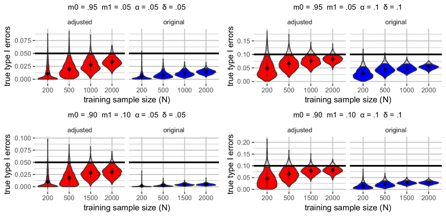
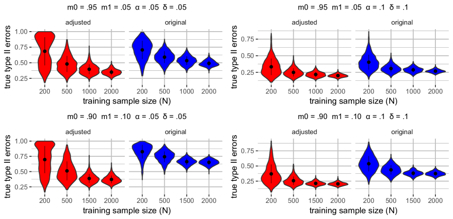
Refer to caption
Figure 5: Violin plots for (approximate) true type I errors of Simulation 1.
Refer to caption
Figure 6: Violin plots for (approximate) true type II errors of Simulation 1.
Refer to caption
Figure 7: Violin plots for (approximate) true type I errors of Simulation 2.
Refer to caption
Figure 8: Violin plots for (approximate) true type II errors of Simulation 2.
Refer to caption
Figure 9: Violin plots for (approximate) true type I errors of Simulation 3.
Refer to caption
Figure 10: Violin plots for (approximate) true type II errors of Simulation 3.

D.4 Tables for Section 5

In this section, we present Table 16 for in Simulation 5 in Section 5.1 and Table 17 for the email spam data analysis in Section 5.2.

Table 16: Averages of (approximate) true type II errors over 1,00010001{,}000 repetitions for Simulation 5 (m0=.95subscript𝑚0.95m_{0}=.95, m1=.05subscript𝑚1.05m_{1}=.05, α=.1𝛼.1\alpha=.1 and δ=.1𝛿.1\delta=.1). Standard errors (×103absentsuperscript103\times 10^{-3}) in parentheses.
algorithms N𝑁N
200200200 500500500 1,00010001{,}000 2,00020002{,}000
T-revision .165(4.32).1654.32.165(4.32) .153(4.08).1534.08.153(4.08) .146(3.52).1463.52.146(3.52) .147(4.27).1474.27.147(4.27)
backward loss correction
(known corruption level)
.151(.77).151.77.151(.77) .139(.70).139.70.139(.70) .161(.71).161.71.161(.71) .199(.69).199.69.199(.69)
backward loss correction
(unknown corruption level)
.158(.02).158.02.158(.02) .163(.02).163.02.163(.02) .186(.01).186.01.186(.01) .192(.01).192.01.192(.01)
Table 17: (Approximate) type I error violation rates, and averages of (approximate) true type II error by benchmark algorithms over 1,00010001{,}000 repetitions for the email spam data. Standard errors (×103absentsuperscript103\times 10^{-3}) in parentheses.
(approximate)
violation rate
average of
(approximate) true
type II errors
T-revision .829(11.91).82911.91.829(11.91) .414(7.01).4147.01.414(7.01)
backward loss correction
(known corruption level)
.831(11.86).83111.86.831(11.86) .573(5.49).5735.49.573(5.49)
backward loss correction
(unknown corruption level)
.750(13.70).75013.70.750(13.70) .631(5.51).6315.51.631(5.51)

D.5 Alternative implementation with a positive ε𝜀\varepsilon

In this section, we repeat the numerical studies for Simulations 1-3 in Section 5 but replace ksuperscript𝑘k^{*} in Algorithm 1 by min{k{1,,n}:αk,δD^+(t(k))αε}:𝑘1𝑛subscript𝛼𝑘𝛿superscript^𝐷subscript𝑡𝑘𝛼𝜀\min\{k\in\{1,\ldots,n\}:\alpha_{k,\delta}-\hat{D}^{+}(t_{(k)})\leq\alpha-\varepsilon\} where ε=0.0001𝜀0.0001\varepsilon=0.0001. The results are presented in Figures 11 - 16. Numerical evidence shows that whether to have a small positive ε𝜀\varepsilon in selection of ksuperscript𝑘k^{*} does not actually affect much the performance of label-noise-adjusted umbrella algorithm. Thus, as a simpler algorithm is always preferred, we recommend taking ε=0𝜀0\varepsilon=0.

Refer to caption
Figure 11: Violin plots for (approximate) true type I errors of Simulation 1.
Refer to caption
Figure 12: Violin plots for (approximate) true type II errors of Simulation 1.
Refer to caption
Figure 13: Violin plots for (approximate) true type I errors of Simulation 2.
Refer to caption
Figure 14: Violin plots for (approximate) true type II errors of Simulation 2.
Refer to caption
Figure 15: Violin plots for (approximate) true type I errors of Simulation 3.
Refer to caption
Figure 16: Violin plots for (approximate) true type II errors of Simulation 3.

E Extra Lemmas

Lemma 4.

Under Assumption 1, for any measurable function T:IRdIR:𝑇superscriptIR𝑑IRT:{\rm I}\kern-1.43994pt{\rm R}^{d}\rightarrow{\rm I}\kern-1.43994pt{\rm R} and arbitrary number zIR𝑧IRz\in{\rm I}\kern-1.43994pt{\rm R}, we have

F~0T(z)=m0F0T(z)+(1m0)F1T(z)  and  F~1T(z)=m1F0T(z)+(1m1)F1T(z).superscriptsubscript~𝐹0𝑇𝑧subscript𝑚0superscriptsubscript𝐹0𝑇𝑧1subscript𝑚0superscriptsubscript𝐹1𝑇𝑧  and  superscriptsubscript~𝐹1𝑇𝑧subscript𝑚1superscriptsubscript𝐹0𝑇𝑧1subscript𝑚1superscriptsubscript𝐹1𝑇𝑧\displaystyle\tilde{F}_{0}^{T}(z)=m_{0}F_{0}^{T}(z)+(1-m_{0})F_{1}^{T}(z)\,\text{ }\text{ and }\text{ }\tilde{F}_{1}^{T}(z)=m_{1}F_{0}^{T}(z)+(1-m_{1})F_{1}^{T}(z)\,.

Furthermore,

IEX~0=m0IEX0+(1m0)IEX1  and  IEX~1=m1IEX0+(1m1)IEX1.IEsuperscript~𝑋0subscript𝑚0IEsuperscript𝑋01subscript𝑚0IEsuperscript𝑋1  and  IEsuperscript~𝑋1subscript𝑚1IEsuperscript𝑋01subscript𝑚1IEsuperscript𝑋1\displaystyle{\rm I}\kern-1.43994pt{\rm E}\tilde{X}^{0}=m_{0}{\rm I}\kern-1.43994pt{\rm E}X^{0}+(1-m_{0}){\rm I}\kern-1.43994pt{\rm E}X^{1}\,\text{ }\text{ and }\text{ }{\rm I}\kern-1.43994pt{\rm E}\tilde{X}^{1}=m_{1}{\rm I}\kern-1.43994pt{\rm E}X^{0}+(1-m_{1}){\rm I}\kern-1.43994pt{\rm E}X^{1}\,.
Proof.

The first two equations can be proved in the similar way. So we will only show the first equation. By Assumption 1, for any Borel set A𝐴A,

P~0(T1(A))subscript~𝑃0superscript𝑇1𝐴\displaystyle\tilde{P}_{0}(T^{-1}(A)) =m0P0(T1(A))+(1m0)P1(T1(A)).absentsubscript𝑚0subscript𝑃0superscript𝑇1𝐴1subscript𝑚0subscript𝑃1superscript𝑇1𝐴\displaystyle=m_{0}P_{0}(T^{-1}(A))+(1-m_{0})P_{1}(T^{-1}(A))\,.

Then, select A=(,z]𝐴𝑧A=(-\infty,z] and the result follows.

Similarly, the proof of last two equations are similar in nature. So we are going to show IEX~0=m0IEX0+(1m0)IEX1IEsuperscript~𝑋0subscript𝑚0IEsuperscript𝑋01subscript𝑚0IEsuperscript𝑋1{\rm I}\kern-1.43994pt{\rm E}\tilde{X}^{0}=m_{0}{\rm I}\kern-1.43994pt{\rm E}X^{0}+(1-m_{0}){\rm I}\kern-1.43994pt{\rm E}X^{1}. Note that by Assumption 1,

IEX~0IEsuperscript~𝑋0\displaystyle{\rm I}\kern-1.43994pt{\rm E}\tilde{X}^{0} =0(1P~0(Xx))𝑑x0P~0(Xx)𝑑xabsentsuperscriptsubscript01subscript~𝑃0𝑋𝑥differential-d𝑥superscriptsubscript0subscript~𝑃0𝑋𝑥differential-d𝑥\displaystyle=\int_{0}^{\infty}(1-\tilde{P}_{0}(X\leq x))dx-\int_{-\infty}^{0}\tilde{P}_{0}(X\leq x)dx
=m0(0(1P0(Xx))𝑑x0P0(Xx)𝑑x)absentsubscript𝑚0superscriptsubscript01subscript𝑃0𝑋𝑥differential-d𝑥superscriptsubscript0subscript𝑃0𝑋𝑥differential-d𝑥\displaystyle=m_{0}\left(\int_{0}^{\infty}(1-P_{0}(X\leq x))dx-\int_{-\infty}^{0}P_{0}(X\leq x)dx\right)
+(1m0)(0(1P1(Xx))𝑑x0P1(Xx)𝑑x)1subscript𝑚0superscriptsubscript01subscript𝑃1𝑋𝑥differential-d𝑥superscriptsubscript0subscript𝑃1𝑋𝑥differential-d𝑥\displaystyle+(1-m_{0})\left(\int_{0}^{\infty}(1-P_{1}(X\leq x))dx-\int_{-\infty}^{0}P_{1}(X\leq x)dx\right)
=m0IEX0+(1m0)IEX1.absentsubscript𝑚0IEsuperscript𝑋01subscript𝑚0IEsuperscript𝑋1\displaystyle=m_{0}{\rm I}\kern-1.43994pt{\rm E}X^{0}+(1-m_{0}){\rm I}\kern-1.43994pt{\rm E}X^{1}\,.

Lemma 5.

For any k{1,,n}𝑘1𝑛k\in\{1,\ldots,n\} and δ(0,1)𝛿01\delta\in(0,1), a unique αk,δsubscript𝛼𝑘𝛿\alpha_{k,\delta} exists. Moreover, under Assumption 2, k=min{k{1,,n}:αk,δα}subscript𝑘:𝑘1𝑛subscript𝛼𝑘𝛿𝛼k_{*}=\min\{k\in\{1,\ldots,n\}:\alpha_{k,\delta}\leq\alpha\}.

Proof.

Let hk(x)=j=kn(nk)xnj(1x)jsubscript𝑘𝑥superscriptsubscript𝑗𝑘𝑛binomial𝑛𝑘superscript𝑥𝑛𝑗superscript1𝑥𝑗h_{k}(x)=\sum_{j=k}^{n}{n\choose k}x^{n-j}(1-x)^{j} for any k{1,,n}𝑘1𝑛k\in\{1,\ldots,n\}. Then, one can show, for kn1𝑘𝑛1k\leq n-1 and x(0,1)𝑥01x\in(0,1),

hk(x)subscriptsuperscript𝑘𝑥\displaystyle h^{\prime}_{k}(x) =j=kn1(nj)(nj)xnj1(1x)jj=knj(nj)xnj(1x)j1absentsuperscriptsubscript𝑗𝑘𝑛1𝑛𝑗binomial𝑛𝑗superscript𝑥𝑛𝑗1superscript1𝑥𝑗superscriptsubscript𝑗𝑘𝑛𝑗binomial𝑛𝑗superscript𝑥𝑛𝑗superscript1𝑥𝑗1\displaystyle=\sum_{j=k}^{n-1}(n-j){n\choose j}x^{n-j-1}(1-x)^{j}-\sum_{j=k}^{n}j{n\choose j}x^{n-j}(1-x)^{j-1}
=ni=k+1n(ni1)xni(1x)i1nj=kn(nj1)xnj(1x)j1absent𝑛superscriptsubscript𝑖𝑘1𝑛binomial𝑛𝑖1superscript𝑥𝑛𝑖superscript1𝑥𝑖1𝑛superscriptsubscript𝑗𝑘𝑛binomial𝑛𝑗1superscript𝑥𝑛𝑗superscript1𝑥𝑗1\displaystyle=n\sum_{i=k+1}^{n}{n\choose i-1}x^{n-i}(1-x)^{i-1}-n\sum_{j=k}^{n}{n\choose j-1}x^{n-j}(1-x)^{j-1}
=n(nk1)xnk(1x)k1,absent𝑛binomial𝑛𝑘1superscript𝑥𝑛𝑘superscript1𝑥𝑘1\displaystyle=-n{n\choose k-1}x^{n-k}(1-x)^{k-1}\,,

which is negative. Thus, hk(x)subscript𝑘𝑥h_{k}(x) is strictly decreasing on (0,1)01(0,1) for kn1𝑘𝑛1k\leq n-1. Furthermore, hn(x)=(1x)nsubscript𝑛𝑥superscript1𝑥𝑛h_{n}(x)=(1-x)^{n} which is also strictly decreasing on (0,1)01(0,1). Since for any k𝑘k, hk(0)=1subscript𝑘01h_{k}(0)=1 and hk(1)=0subscript𝑘10h_{k}(1)=0, there exists a unique αk,δsubscript𝛼𝑘𝛿\alpha_{k,\delta} such that hk(αk,δ)=δsubscript𝑘subscript𝛼𝑘𝛿𝛿h_{k}(\alpha_{k,\delta})=\delta.

Recall that ksubscript𝑘k_{*} is defined as the smallest k𝑘k such that hk(α)δsubscript𝑘𝛼𝛿h_{k}(\alpha)\leq\delta. Meanwhile, by monotonicity, for any k𝑘k, the inequality hk(α)δsubscript𝑘𝛼𝛿h_{k}(\alpha)\leq\delta is equivalent to αk,δαsubscript𝛼𝑘𝛿𝛼\alpha_{k,\delta}\leq\alpha. Assumption 2 guarantees the existence of k𝑘k such that hk(α)subscript𝑘𝛼h_{k}(\alpha). Therefore it also guarantees the existence of k𝑘k such that αk,δαsubscript𝛼𝑘𝛿𝛼\alpha_{k,\delta}\leq\alpha. Then, for any δ𝛿\delta, {k{1,,n}:hk(α)δ}={k{1,,n}:αk,δα}conditional-set𝑘1𝑛subscript𝑘𝛼𝛿conditional-set𝑘1𝑛subscript𝛼𝑘𝛿𝛼\{k\in\{1,\ldots,n\}:h_{k}(\alpha)\leq\delta\}=\{k\in\{1,\ldots,n\}:\alpha_{k,\delta}\leq\alpha\}. Then, k=min{k{1,,n}:αk,δα}subscript𝑘:𝑘1𝑛subscript𝛼𝑘𝛿𝛼k_{*}=\min\{k\in\{1,\ldots,n\}:\alpha_{k,\delta}\leq\alpha\}. ∎

Lemma 6.

Given a random variable XIRd𝑋superscriptIR𝑑X\in{\rm I}\kern-1.43994pt{\rm R}^{d} with probability measure P𝑃P and a deterministic measurable function T:IRdIR:𝑇superscriptIR𝑑IRT:{\rm I}\kern-1.43994pt{\rm R}^{d}\rightarrow{\rm I}\kern-1.43994pt{\rm R}, define probability measure PT(B)=P(T(X)B)superscript𝑃𝑇𝐵𝑃𝑇𝑋𝐵P^{T}(B)=P(T(X)\in B) for any Borel set B𝐵B. Furthermore, denote the distribution functions of P𝑃P and PTsuperscript𝑃𝑇P^{T} as F𝐹F and FTsuperscript𝐹𝑇F^{T}, respectively. Let X1,X2,,XnXsimilar-tosubscript𝑋1subscript𝑋2subscript𝑋𝑛𝑋X_{1},X_{2},\ldots,X_{n}\sim X be i.i.d. random variables. Moreover, let F^T(z)=1nj=1n1I{T(Xj)z}superscript^𝐹𝑇𝑧1𝑛superscriptsubscript𝑗1𝑛1I𝑇subscript𝑋𝑗𝑧\hat{F}^{T}(z)=\frac{1}{n}\sum_{j=1}^{n}{\rm 1}\kern-1.92004pt{\rm I}\{T(X_{j})\leq z\} for any zIR𝑧IRz\in{\rm I}\kern-1.43994pt{\rm R}. Then, for any ξ>0𝜉0\xi>0

P(supzIR|F^T(z)FT(z)|>ξ)2e2nξ2.𝑃subscriptsupremum𝑧IRsuperscript^𝐹𝑇𝑧superscript𝐹𝑇𝑧𝜉2superscript𝑒2𝑛superscript𝜉2\displaystyle P\left(\sup_{z\in{\rm I}\kern-1.00795pt{\rm R}}\left|\hat{F}^{T}(z)-F^{T}(z)\right|>\xi\right)\leq 2e^{-2n\xi^{2}}\,.
Proof.

Note that X1,X2,,Xnsubscript𝑋1subscript𝑋2subscript𝑋𝑛X_{1},X_{2},\ldots,X_{n} are i.i.d. random variables, then so are T(X1),T(X2),,T(Xn)𝑇subscript𝑋1𝑇subscript𝑋2𝑇subscript𝑋𝑛T(X_{1}),T(X_{2}),\ldots,T(X_{n}). Denote Tj=T(Xj)subscript𝑇𝑗𝑇subscript𝑋𝑗T_{j}=T(X_{j}), then Tjsubscript𝑇𝑗T_{j} has the probability measure PTsuperscript𝑃𝑇P^{T}. Note that the Dvoretsky-Kiefer-Wolfowitz inequality says,

PT(supzIR|1nj=1n1I{Tjz}FT(z)|>ξ)2e2nξ2.superscript𝑃𝑇subscriptsupremum𝑧IR1𝑛superscriptsubscript𝑗1𝑛1Isubscript𝑇𝑗𝑧superscript𝐹𝑇𝑧𝜉2superscript𝑒2𝑛superscript𝜉2\displaystyle P^{T}\left(\sup_{z\in{\rm I}\kern-1.00795pt{\rm R}}\left|\frac{1}{n}\sum_{j=1}^{n}{\rm 1}\kern-1.92004pt{\rm I}\{T_{j}\leq z\}-F^{T}(z)\right|>\xi\right)\leq 2e^{-2n\xi^{2}}\,.

Then, it suffices to show the left hand side of above inequality equals P(supzIR|F^T(z)FT(z)|>ξ)𝑃subscriptsupremum𝑧IRsuperscript^𝐹𝑇𝑧superscript𝐹𝑇𝑧𝜉P\left(\sup_{z\in{\rm I}\kern-1.00795pt{\rm R}}\left|\hat{F}^{T}(z)-F^{T}(z)\right|>\xi\right). Towards that, denote

fn(x1,x2,,xn)=1I{supzIR|1nj=1n1I{T(xj)z}FT(z)|>ξ},subscript𝑓𝑛subscript𝑥1subscript𝑥2subscript𝑥𝑛1Isubscriptsupremum𝑧IR1𝑛superscriptsubscript𝑗1𝑛1I𝑇subscript𝑥𝑗𝑧superscript𝐹𝑇𝑧𝜉\displaystyle f_{n}(x_{1},x_{2},\ldots,x_{n})={\rm 1}\kern-1.92004pt{\rm I}\left\{\sup_{z\in{\rm I}\kern-1.00795pt{\rm R}}\left|\frac{1}{n}\sum_{j=1}^{n}{\rm 1}\kern-1.92004pt{\rm I}\{T(x_{j})\leq z\}-F^{T}(z)\right|>\xi\right\}\,,

and

f0(t1,t2,,tn)=1I{supzIR|1nj=1n1I{tjz}FT(z)|>ξ}.subscript𝑓0subscript𝑡1subscript𝑡2subscript𝑡𝑛1Isubscriptsupremum𝑧IR1𝑛superscriptsubscript𝑗1𝑛1Isubscript𝑡𝑗𝑧superscript𝐹𝑇𝑧𝜉\displaystyle f_{0}(t_{1},t_{2},\ldots,t_{n})={\rm 1}\kern-1.92004pt{\rm I}\left\{\sup_{z\in{\rm I}\kern-1.00795pt{\rm R}}\left|\frac{1}{n}\sum_{j=1}^{n}{\rm 1}\kern-1.92004pt{\rm I}\{t_{j}\leq z\}-F^{T}(z)\right|>\xi\right\}\,.

By Fubini’s theorem, it holds that

P(supzIR|F^T(z)FT(z)|>ξ)=IE1IE2IEnfn(X1,X2,,Xn),𝑃subscriptsupremum𝑧IRsuperscript^𝐹𝑇𝑧superscript𝐹𝑇𝑧𝜉subscriptIE1subscriptIE2subscriptIE𝑛subscript𝑓𝑛subscript𝑋1subscript𝑋2subscript𝑋𝑛\displaystyle P\left(\sup_{z\in{\rm I}\kern-1.00795pt{\rm R}}\left|\hat{F}^{T}(z)-F^{T}(z)\right|>\xi\right)={\rm I}\kern-1.43994pt{\rm E}_{1}{\rm I}\kern-1.43994pt{\rm E}_{2}\ldots{\rm I}\kern-1.43994pt{\rm E}_{n}f_{n}(X_{1},X_{2},\ldots,X_{n})\,,

and

PT(supzIR|1nj=1n1I{Tjz}FT(z)|>ξ)=IE1TIE2TIEnTf0(T1,T2,,Tn),superscript𝑃𝑇subscriptsupremum𝑧IR1𝑛superscriptsubscript𝑗1𝑛1Isubscript𝑇𝑗𝑧superscript𝐹𝑇𝑧𝜉subscriptsuperscriptIE𝑇1subscriptsuperscriptIE𝑇2subscriptsuperscriptIE𝑇𝑛subscript𝑓0subscript𝑇1subscript𝑇2subscript𝑇𝑛\displaystyle P^{T}\left(\sup_{z\in{\rm I}\kern-1.00795pt{\rm R}}\left|\frac{1}{n}\sum_{j=1}^{n}{\rm 1}\kern-1.92004pt{\rm I}\{T_{j}\leq z\}-F^{T}(z)\right|>\xi\right)={\rm I}\kern-1.43994pt{\rm E}^{T}_{1}{\rm I}\kern-1.43994pt{\rm E}^{T}_{2}\ldots{\rm I}\kern-1.43994pt{\rm E}^{T}_{n}f_{0}(T_{1},T_{2},\ldots,T_{n})\,,

where IEjsubscriptIE𝑗{\rm I}\kern-1.43994pt{\rm E}_{j} and IEjTsuperscriptsubscriptIE𝑗𝑇{\rm I}\kern-1.43994pt{\rm E}_{j}^{T} are the expectations taken with respect to Xjsubscript𝑋𝑗X_{j} and Tjsubscript𝑇𝑗T_{j} under the probability measures P𝑃P and PTsuperscript𝑃𝑇P^{T}, respectively. Thus, it suffices to show

IE1IE2IEnfn(X1,X2,,Xn)=IE1TIE2TIEnTf0(T1,T2,,Tn),subscriptIE1subscriptIE2subscriptIE𝑛subscript𝑓𝑛subscript𝑋1subscript𝑋2subscript𝑋𝑛subscriptsuperscriptIE𝑇1subscriptsuperscriptIE𝑇2subscriptsuperscriptIE𝑇𝑛subscript𝑓0subscript𝑇1subscript𝑇2subscript𝑇𝑛\displaystyle{\rm I}\kern-1.43994pt{\rm E}_{1}{\rm I}\kern-1.43994pt{\rm E}_{2}\ldots{\rm I}\kern-1.43994pt{\rm E}_{n}f_{n}(X_{1},X_{2},\ldots,X_{n})={\rm I}\kern-1.43994pt{\rm E}^{T}_{1}{\rm I}\kern-1.43994pt{\rm E}^{T}_{2}\ldots{\rm I}\kern-1.43994pt{\rm E}^{T}_{n}f_{0}(T_{1},T_{2},\ldots,T_{n})\,,

and we will show this by induction. Denote

fl(x1,x2,,xl,tl+1,tl+2,,tn)=1I{supzIR|1n(j=1l1I{T(xj)z}+j=l+1n1I{tjz})FT(z)|>ξ},subscript𝑓𝑙subscript𝑥1subscript𝑥2subscript𝑥𝑙subscript𝑡𝑙1subscript𝑡𝑙2subscript𝑡𝑛1Isubscriptsupremum𝑧IR1𝑛superscriptsubscript𝑗1𝑙1I𝑇subscript𝑥𝑗𝑧superscriptsubscript𝑗𝑙1𝑛1Isubscript𝑡𝑗𝑧superscript𝐹𝑇𝑧𝜉\displaystyle f_{l}(x_{1},x_{2},\ldots,x_{l},t_{l+1},t_{l+2},\ldots,t_{n})={\rm 1}\kern-1.92004pt{\rm I}\left\{\sup_{z\in{\rm I}\kern-1.00795pt{\rm R}}\left|\frac{1}{n}\left(\sum_{j=1}^{l}{\rm 1}\kern-1.92004pt{\rm I}\{T(x_{j})\leq z\}+\sum_{j=l+1}^{n}{\rm 1}\kern-1.92004pt{\rm I}\{t_{j}\leq z\}\right)-F^{T}(z)\right|>\xi\right\}\,,

for any l{1,2,,n1}𝑙12𝑛1l\in\{1,2,\ldots,n-1\} and An1(x1,x2,,xn1)={tn:fn1(x1,x2,,xn1,tn)=1}subscript𝐴𝑛1subscript𝑥1subscript𝑥2subscript𝑥𝑛1conditional-setsubscript𝑡𝑛subscript𝑓𝑛1subscript𝑥1subscript𝑥2subscript𝑥𝑛1subscript𝑡𝑛1A_{n-1}(x_{1},x_{2},\ldots,x_{n-1})=\left\{t_{n}:f_{n-1}(x_{1},x_{2},\ldots,x_{n-1},t_{n})=1\right\}. Then, for any fixed values of x1,x2,,xn1subscript𝑥1subscript𝑥2subscript𝑥𝑛1x_{1},x_{2},\ldots,x_{n-1},

IEnfn(x1,x2,,xn1,Xn)subscriptIE𝑛subscript𝑓𝑛subscript𝑥1subscript𝑥2subscript𝑥𝑛1subscript𝑋𝑛\displaystyle{\rm I}\kern-1.43994pt{\rm E}_{n}f_{n}(x_{1},x_{2},\ldots,x_{n-1},X_{n}) =P(T(Xn)An1(x1,x2,,xn1))absent𝑃𝑇subscript𝑋𝑛subscript𝐴𝑛1subscript𝑥1subscript𝑥2subscript𝑥𝑛1\displaystyle=P(T(X_{n})\in A_{n-1}(x_{1},x_{2},\ldots,x_{n-1}))
=PT(An1(x1,x2,,xn1))absentsuperscript𝑃𝑇subscript𝐴𝑛1subscript𝑥1subscript𝑥2subscript𝑥𝑛1\displaystyle=P^{T}(A_{n-1}(x_{1},x_{2},\ldots,x_{n-1}))
=IEnTfn1(x1,x2,,xn1,Tn),absentsuperscriptsubscriptIE𝑛𝑇subscript𝑓𝑛1subscript𝑥1subscript𝑥2subscript𝑥𝑛1subscript𝑇𝑛\displaystyle={\rm I}\kern-1.43994pt{\rm E}_{n}^{T}f_{n-1}(x_{1},x_{2},\ldots,x_{n-1},T_{n})\,,

and thus,

IE1IE2IEnfn(X1,X2,,Xn)=IE1TIE2TIEn1IEnTfn1(X1,X2,,Xn1,Tn).subscriptIE1subscriptIE2subscriptIE𝑛subscript𝑓𝑛subscript𝑋1subscript𝑋2subscript𝑋𝑛subscriptsuperscriptIE𝑇1subscriptsuperscriptIE𝑇2subscriptIE𝑛1subscriptsuperscriptIE𝑇𝑛subscript𝑓𝑛1subscript𝑋1subscript𝑋2subscript𝑋𝑛1subscript𝑇𝑛\displaystyle{\rm I}\kern-1.43994pt{\rm E}_{1}{\rm I}\kern-1.43994pt{\rm E}_{2}\ldots{\rm I}\kern-1.43994pt{\rm E}_{n}f_{n}(X_{1},X_{2},\ldots,X_{n})={\rm I}\kern-1.43994pt{\rm E}^{T}_{1}{\rm I}\kern-1.43994pt{\rm E}^{T}_{2}\ldots{\rm I}\kern-1.43994pt{\rm E}_{n-1}{\rm I}\kern-1.43994pt{\rm E}^{T}_{n}f_{n-1}(X_{1},X_{2},\ldots,X_{n-1},T_{n})\,.

Now, assume that for some l{2,3,,n}𝑙23𝑛l\in\{2,3,\ldots,n\},

IE1IE2IEnfn(X1,X2,,Xn)=IE1IE2IEl1IElTIEl+1TIEnTfl1(X1,X2,,Xl1,Tl,Tl+1,,Tn).subscriptIE1subscriptIE2subscriptIE𝑛subscript𝑓𝑛subscript𝑋1subscript𝑋2subscript𝑋𝑛subscriptIE1subscriptIE2subscriptIE𝑙1subscriptsuperscriptIE𝑇𝑙subscriptsuperscriptIE𝑇𝑙1subscriptsuperscriptIE𝑇𝑛subscript𝑓𝑙1subscript𝑋1subscript𝑋2subscript𝑋𝑙1subscript𝑇𝑙subscript𝑇𝑙1subscript𝑇𝑛{\rm I}\kern-1.43994pt{\rm E}_{1}{\rm I}\kern-1.43994pt{\rm E}_{2}\ldots{\rm I}\kern-1.43994pt{\rm E}_{n}f_{n}(X_{1},X_{2},\ldots,X_{n})\\ ={\rm I}\kern-1.43994pt{\rm E}_{1}{\rm I}\kern-1.43994pt{\rm E}_{2}\ldots{\rm I}\kern-1.43994pt{\rm E}_{l-1}{\rm I}\kern-1.43994pt{\rm E}^{T}_{l}{\rm I}\kern-1.43994pt{\rm E}^{T}_{l+1}\ldots{\rm I}\kern-1.43994pt{\rm E}^{T}_{n}f_{l-1}(X_{1},X_{2},\ldots,X_{l-1},T_{l},T_{l+1},\ldots,T_{n})\,.

Therefore, for any fixed values of x1,x2,,xl2subscript𝑥1subscript𝑥2subscript𝑥𝑙2x_{1},x_{2},\ldots,x_{l-2}, denote

Al2(x1,x2,,xl2)={tl1:IElTIEl+1TIEnTfl2(x1,x2,,xt2,tl1,Tl,,Tn)=1},subscript𝐴𝑙2subscript𝑥1subscript𝑥2subscript𝑥𝑙2conditional-setsubscript𝑡𝑙1subscriptsuperscriptIE𝑇𝑙subscriptsuperscriptIE𝑇𝑙1subscriptsuperscriptIE𝑇𝑛subscript𝑓𝑙2subscript𝑥1subscript𝑥2subscript𝑥𝑡2subscript𝑡𝑙1subscript𝑇𝑙subscript𝑇𝑛1\displaystyle A_{l-2}(x_{1},x_{2},\ldots,x_{l-2})=\{t_{l-1}:{\rm I}\kern-1.43994pt{\rm E}^{T}_{l}{\rm I}\kern-1.43994pt{\rm E}^{T}_{l+1}\ldots{\rm I}\kern-1.43994pt{\rm E}^{T}_{n}f_{l-2}(x_{1},x_{2},\ldots,x_{t-2},t_{l-1},T_{l},\ldots,T_{n})=1\}\,,

we can have

IEl1IElTIEl+1TIEnTfl1(x1,x2,,xl2,Xl1,Tl,Tl+1,,Tn)=P(T(Xl1)Al2(x1,x2,,xl2))=PT(Al2(x1,x2,,xl2)),subscriptIE𝑙1subscriptsuperscriptIE𝑇𝑙subscriptsuperscriptIE𝑇𝑙1subscriptsuperscriptIE𝑇𝑛subscript𝑓𝑙1subscript𝑥1subscript𝑥2subscript𝑥𝑙2subscript𝑋𝑙1subscript𝑇𝑙subscript𝑇𝑙1subscript𝑇𝑛𝑃𝑇subscript𝑋𝑙1subscript𝐴𝑙2subscript𝑥1subscript𝑥2subscript𝑥𝑙2superscript𝑃𝑇subscript𝐴𝑙2subscript𝑥1subscript𝑥2subscript𝑥𝑙2{\rm I}\kern-1.43994pt{\rm E}_{l-1}{\rm I}\kern-1.43994pt{\rm E}^{T}_{l}{\rm I}\kern-1.43994pt{\rm E}^{T}_{l+1}\ldots{\rm I}\kern-1.43994pt{\rm E}^{T}_{n}f_{l-1}(x_{1},x_{2},\ldots,x_{l-2},X_{l-1},T_{l},T_{l+1},\ldots,T_{n})\\ =P(T(X_{l-1})\in A_{l-2}(x_{1},x_{2},\ldots,x_{l-2}))=P^{T}(A_{l-2}(x_{1},x_{2},\ldots,x_{l-2}))\,,

and thus,

IEl1IElTIEl+1TIEnTfl1(x1,x2,,xl2,Xl1,Tl,Tl+1,,Tn)=IEl1TIElTIEnTfl2(x1,x2,,xt2,Tl1,,Tn).subscriptIE𝑙1subscriptsuperscriptIE𝑇𝑙subscriptsuperscriptIE𝑇𝑙1subscriptsuperscriptIE𝑇𝑛subscript𝑓𝑙1subscript𝑥1subscript𝑥2subscript𝑥𝑙2subscript𝑋𝑙1subscript𝑇𝑙subscript𝑇𝑙1subscript𝑇𝑛superscriptsubscriptIE𝑙1𝑇subscriptsuperscriptIE𝑇𝑙subscriptsuperscriptIE𝑇𝑛subscript𝑓𝑙2subscript𝑥1subscript𝑥2subscript𝑥𝑡2subscript𝑇𝑙1subscript𝑇𝑛{\rm I}\kern-1.43994pt{\rm E}_{l-1}{\rm I}\kern-1.43994pt{\rm E}^{T}_{l}{\rm I}\kern-1.43994pt{\rm E}^{T}_{l+1}\ldots{\rm I}\kern-1.43994pt{\rm E}^{T}_{n}f_{l-1}(x_{1},x_{2},\ldots,x_{l-2},X_{l-1},T_{l},T_{l+1},\ldots,T_{n})\\ ={\rm I}\kern-1.43994pt{\rm E}_{l-1}^{T}{\rm I}\kern-1.43994pt{\rm E}^{T}_{l}\ldots{\rm I}\kern-1.43994pt{\rm E}^{T}_{n}f_{l-2}(x_{1},x_{2},\ldots,x_{t-2},T_{l-1},\ldots,T_{n})\,.

Therefore, by the assumption, we have

IE1IE2IEnfn(X1,X2,,Xn)=IE1IE2IEl2IEl1TIElTIEnTfl2(X1,X2,,Xl2,Tl1,Tl,,Tn).subscriptIE1subscriptIE2subscriptIE𝑛subscript𝑓𝑛subscript𝑋1subscript𝑋2subscript𝑋𝑛subscriptIE1subscriptIE2subscriptIE𝑙2subscriptsuperscriptIE𝑇𝑙1subscriptsuperscriptIE𝑇𝑙subscriptsuperscriptIE𝑇𝑛subscript𝑓𝑙2subscript𝑋1subscript𝑋2subscript𝑋𝑙2subscript𝑇𝑙1subscript𝑇𝑙subscript𝑇𝑛{\rm I}\kern-1.43994pt{\rm E}_{1}{\rm I}\kern-1.43994pt{\rm E}_{2}\ldots{\rm I}\kern-1.43994pt{\rm E}_{n}f_{n}(X_{1},X_{2},\ldots,X_{n})\\ ={\rm I}\kern-1.43994pt{\rm E}_{1}{\rm I}\kern-1.43994pt{\rm E}_{2}\ldots{\rm I}\kern-1.43994pt{\rm E}_{l-2}{\rm I}\kern-1.43994pt{\rm E}^{T}_{l-1}{\rm I}\kern-1.43994pt{\rm E}^{T}_{l}\ldots{\rm I}\kern-1.43994pt{\rm E}^{T}_{n}f_{l-2}(X_{1},X_{2},\ldots,X_{l-2},T_{l-1},T_{l},\ldots,T_{n})\,.

We conclude the proof by induction. ∎

F Proofs

Lemma 1.

Let’s focus on the event of the statement of Assumption 3, whose complement holds with probability at most δ1(nb)subscript𝛿1subscript𝑛b\delta_{1}(n_{\text{b}}). Meanwhile, by Lemma 4, for any zIR𝑧IRz\in{\rm I}\kern-1.43994pt{\rm R},

F~0T^(z)F~1T^(z)subscriptsuperscript~𝐹^𝑇0𝑧subscriptsuperscript~𝐹^𝑇1𝑧\displaystyle\tilde{F}^{\hat{T}}_{0}\left(z\right)-\tilde{F}^{\hat{T}}_{1}\left(z\right) =[m0F0T^(z)+(1m0)F1T^(z)][m1F0T^(z)+(1m1)F1T^(z)]absentdelimited-[]subscript𝑚0subscriptsuperscript𝐹^𝑇0𝑧1subscript𝑚0subscriptsuperscript𝐹^𝑇1𝑧delimited-[]subscript𝑚1subscriptsuperscript𝐹^𝑇0𝑧1subscript𝑚1subscriptsuperscript𝐹^𝑇1𝑧\displaystyle=\left[m_{0}F^{\hat{T}}_{0}(z)+(1-m_{0})F^{\hat{T}}_{1}(z)\right]-\left[m_{1}F^{\hat{T}}_{0}(z)+(1-m_{1})F^{\hat{T}}_{1}(z)\right]
=(m0m1)(F0T^(z)F1T^(z)).absentsubscript𝑚0subscript𝑚1subscriptsuperscript𝐹^𝑇0𝑧subscriptsuperscript𝐹^𝑇1𝑧\displaystyle=(m_{0}-m_{1})\left(F^{\hat{T}}_{0}(z)-F^{\hat{T}}_{1}(z)\right)\,.

Furthermore, for any classifier ϕ(X)=1I{T^(X)>z}italic-ϕ𝑋1I^𝑇𝑋𝑧\phi(X)={\rm 1}\kern-1.92004pt{\rm I}\{\hat{T}(X)>z\}

R~0(ϕ)R0(ϕ)subscript~𝑅0italic-ϕsubscript𝑅0italic-ϕ\displaystyle\tilde{R}_{0}(\phi)-R_{0}(\phi) =(1F~0T^(z))(1F0T^(z))absent1subscriptsuperscript~𝐹^𝑇0𝑧1subscriptsuperscript𝐹^𝑇0𝑧\displaystyle=\left(1-\tilde{F}^{\hat{T}}_{0}\left(z\right)\right)-\left(1-F^{\hat{T}}_{0}\left(z\right)\right)
=F0T^(z)m0F0T^(z)(1m0)F1T^(z)absentsubscriptsuperscript𝐹^𝑇0𝑧subscript𝑚0subscriptsuperscript𝐹^𝑇0𝑧1subscript𝑚0subscriptsuperscript𝐹^𝑇1𝑧\displaystyle=F^{\hat{T}}_{0}\left(z\right)-m_{0}F^{\hat{T}}_{0}(z)-(1-m_{0})F^{\hat{T}}_{1}(z)
=(1m0)(F0T^(z)F1T^(z)),absent1subscript𝑚0subscriptsuperscript𝐹^𝑇0𝑧subscriptsuperscript𝐹^𝑇1𝑧\displaystyle=(1-m_{0})\left(F^{\hat{T}}_{0}(z)-F^{\hat{T}}_{1}(z)\right)\,,

which is positive by Assumption 3. Now, let D(z)=R~0(ϕ)R0(ϕ)>0𝐷𝑧subscript~𝑅0italic-ϕsubscript𝑅0italic-ϕ0D(z)=\tilde{R}_{0}(\phi)-R_{0}(\phi)>0 and therefore R0(ϕ^k)>αD(t(k))subscript𝑅0subscript^italic-ϕsubscript𝑘𝛼𝐷subscript𝑡subscript𝑘R_{0}(\hat{\phi}_{k_{*}})>\alpha-D(t_{(k_{*})}) is equivalent to R~0(ϕ^k)>αsubscript~𝑅0subscript^italic-ϕsubscript𝑘𝛼\tilde{R}_{0}(\hat{\phi}_{k_{*}})>\alpha, whose probability is δ𝛿\delta by Proposition 1. To this end, we have shown

IP(R0(ϕ^k)>αD(t(k)))δ+δ1(nb).IPsubscript𝑅0subscript^italic-ϕsubscript𝑘𝛼𝐷subscript𝑡subscript𝑘𝛿subscript𝛿1subscript𝑛b\displaystyle{\rm I}\kern-1.43994pt{\rm P}\left(R_{0}(\hat{\phi}_{k_{*}})>\alpha-D(t_{(k_{*})})\right)\leq\delta+\delta_{1}(n_{\text{b}})\,.

Proof of Lemma 2.

By Lemma 5, the set {k{1,,n}:αk,δα}conditional-set𝑘1𝑛subscript𝛼𝑘𝛿𝛼\{k\in\{1,\ldots,n\}:\alpha_{k,\delta}\leq\alpha\} is non-empty. Then, the set {k{1,,n}:αk,δD^+(t(k))α}conditional-set𝑘1𝑛subscript𝛼𝑘𝛿superscript^𝐷subscript𝑡𝑘𝛼\{k\in\{1,\ldots,n\}:\alpha_{k,\delta}-\hat{D}^{+}(t_{(k)})\leq\alpha\} is non-empty since D^+(t(k))superscript^𝐷subscript𝑡𝑘\hat{D}^{+}(t_{(k)}) is non-negative. Then k=min{k{1,,n}:αk,δD^+(t(k))α}superscript𝑘:𝑘1𝑛subscript𝛼𝑘𝛿superscript^𝐷subscript𝑡𝑘𝛼k^{*}=\min\{k\in\{1,\ldots,n\}:\alpha_{k,\delta}-\hat{D}^{+}(t_{(k)})\leq\alpha\} exists. Note that k=min{k{1,,n}:αk,δα}subscript𝑘:𝑘1𝑛subscript𝛼𝑘𝛿𝛼k_{*}=\min\{k\in\{1,\ldots,n\}:\alpha_{k,\delta}\leq\alpha\} by Lemma 5. Since {k{1,,n}:αk,δα}conditional-set𝑘1𝑛subscript𝛼𝑘𝛿𝛼\{k\in\{1,\ldots,n\}:\alpha_{k,\delta}\leq\alpha\} is a subset of {k{1,,n}:αk,δD^+(t(k))α}conditional-set𝑘1𝑛subscript𝛼𝑘𝛿superscript^𝐷subscript𝑡𝑘𝛼\{k\in\{1,\ldots,n\}:\alpha_{k,\delta}-\hat{D}^{+}(t_{(k)})\leq\alpha\} by the non-negativeness of D^+superscript^𝐷\hat{D}^{+}, it can be concluded that kksuperscript𝑘subscript𝑘k^{*}\leq k_{*}. ∎

Proof of Lemma 3.

Assumption 1 implies 0M#:=1m0#m0#m1#M=1m0m0m10subscript𝑀#assign1superscriptsubscript𝑚0#superscriptsubscript𝑚0#superscriptsubscript𝑚1#𝑀1subscript𝑚0subscript𝑚0subscript𝑚10\leq M_{\#}:=\frac{1-m_{0}^{\#}}{m_{0}^{\#}-m_{1}^{\#}}\leq M=\frac{1-m_{0}}{m_{0}-m_{1}}, and thus, 0D^#+(c)D^+(c)0subscriptsuperscript^𝐷#𝑐superscript^𝐷𝑐0\leq\hat{D}^{+}_{\#}(c)\leq\hat{D}^{+}(c). Then, {k{1,,n}:αk,δα}conditional-set𝑘1𝑛subscript𝛼𝑘𝛿𝛼\{k\in\{1,\ldots,n\}:\alpha_{k,\delta}\leq\alpha\}, which is non-empty by Assumption 2, is a subset of {k{1,,n}:αk,δD^#+(t(k))α}conditional-set𝑘1𝑛subscript𝛼𝑘𝛿subscriptsuperscript^𝐷#subscript𝑡𝑘𝛼\{k\in\{1,\ldots,n\}:\alpha_{k,\delta}-\hat{D}^{+}_{\#}(t_{(k)})\leq\alpha\}. This implies k#subscriptsuperscript𝑘#k^{*}_{\#} exists and is smaller than or equal to ksubscript𝑘k_{*}. Furthermore, {k{1,,n}:αk,δD^#+(t(k))α}conditional-set𝑘1𝑛subscript𝛼𝑘𝛿subscriptsuperscript^𝐷#subscript𝑡𝑘𝛼\{k\in\{1,\ldots,n\}:\alpha_{k,\delta}-\hat{D}^{+}_{\#}(t_{(k)})\leq\alpha\} is also a subset of {k{1,,n}:αk,δD^+(t(k))α}conditional-set𝑘1𝑛subscript𝛼𝑘𝛿superscript^𝐷subscript𝑡𝑘𝛼\{k\in\{1,\ldots,n\}:\alpha_{k,\delta}-\hat{D}^{+}(t_{(k)})\leq\alpha\} and thus, k#=min{k{1,,n}:αk,δD^#+(t(k))α}subscriptsuperscript𝑘#:𝑘1𝑛subscript𝛼𝑘𝛿subscriptsuperscript^𝐷#subscript𝑡𝑘𝛼k^{*}_{\#}=\min\{k\in\{1,\ldots,n\}:\alpha_{k,\delta}-\hat{D}^{+}_{\#}(t_{(k)})\leq\alpha\} is larger than or equal to ksuperscript𝑘k^{*}. ∎

Proof of Theorem 1.

Let’s focus on the event where statement of both Assumption 3 and 4 hold, whose complement has probability less that δ1(nb)+δ2(nb)subscript𝛿1subscript𝑛bsubscript𝛿2subscript𝑛b\delta_{1}(n_{\text{b}})+\delta_{2}(n_{\text{b}}). Then, let

e={supzIR|D^(z)D(z)|21ε}.subscriptesubscriptsupremum𝑧IR^𝐷𝑧𝐷𝑧superscript21𝜀\displaystyle\mathcal{B}_{\emph{\text{e}}}=\left\{\sup_{z\in{\rm I}\kern-1.00795pt{\rm R}}\left|\hat{D}(z)-D(z)\right|\leq 2^{-1}\varepsilon\right\}\,.

It follows from Lemma 6 that

IP(ec)IPsuperscriptsubscripte𝑐\displaystyle{\rm I}\kern-1.43994pt{\rm P}(\mathcal{B}_{\emph{\text{e}}}^{c}) IP(supzIR|F~^0T^(z)F~0T^(z)|>ε4)+IP(supzIR|F~^1T^(z)F~1T^(z)|>ε4)absentIPsubscriptsupremum𝑧IRsubscriptsuperscript^~𝐹^𝑇0𝑧subscriptsuperscript~𝐹^𝑇0𝑧𝜀4IPsubscriptsupremum𝑧IRsubscriptsuperscript^~𝐹^𝑇1𝑧subscriptsuperscript~𝐹^𝑇1𝑧𝜀4\displaystyle\leq{\rm I}\kern-1.43994pt{\rm P}\left(\sup_{z\in{\rm I}\kern-1.00795pt{\rm R}}\left|\hat{\tilde{F}}^{\hat{T}}_{0}(z)-\tilde{F}^{\hat{T}}_{0}(z)\right|>\frac{\varepsilon}{4}\right)+{\rm I}\kern-1.43994pt{\rm P}\left(\sup_{z\in{\rm I}\kern-1.00795pt{\rm R}}\left|\hat{\tilde{F}}^{\hat{T}}_{1}(z)-\tilde{F}^{\hat{T}}_{1}(z)\right|>\frac{\varepsilon}{4}\right)
2e81ne0M2ε2+2e81ne1M2ε2.absent2superscript𝑒superscript81subscriptsuperscript𝑛0esuperscript𝑀2superscript𝜀22superscript𝑒superscript81subscriptsuperscript𝑛1esuperscript𝑀2superscript𝜀2\displaystyle\leq 2e^{-8^{-1}n^{0}_{\text{e}}M^{-2}\varepsilon^{2}}+2e^{-8^{-1}n^{1}_{\text{e}}M^{-2}\varepsilon^{2}}\,.

Note that since D(z)𝐷𝑧D(z) is non-negative by Lemma 1, |D^+(z)D(z)||D^(z)D(z)|21εsuperscript^𝐷𝑧𝐷𝑧^𝐷𝑧𝐷𝑧superscript21𝜀\left|\hat{D}^{+}(z)-D(z)\right|\leq\left|\hat{D}(z)-D(z)\right|\leq 2^{-1}\varepsilon on esubscripte\mathcal{B}_{\emph{\text{e}}}. So, one can conclude that on the event esubscripte\mathcal{B}_{\emph{\text{e}}}, ksuperscript𝑘k^{*} is chosen from all k𝑘k such that αk,δD(t(k))α21εsubscript𝛼𝑘𝛿𝐷subscript𝑡𝑘𝛼superscript21𝜀\alpha_{k,\delta}-D(t_{(k)})\leq\alpha-2^{-1}\varepsilon. Furthermore, denote ck=inf{y:F~0T^(y)kn1}subscript𝑐𝑘infimumconditional-set𝑦subscriptsuperscript~𝐹^𝑇0𝑦𝑘superscript𝑛1c_{k}=\inf\{y:\tilde{F}^{\hat{T}}_{0}(y)\geq kn^{-1}\} and k0=min{k{1,,n}:αk,δD(ck)α41ε}subscript𝑘0:𝑘1𝑛subscript𝛼𝑘𝛿𝐷subscript𝑐𝑘𝛼superscript41𝜀k_{0}=\min\{k\in\{1,\ldots,n\}:\alpha_{k,\delta}-D(c_{k})\leq\alpha-4^{-1}\varepsilon\}. Note that since 𝒟Tsubscript𝒟𝑇\mathcal{D}_{T} is a closed interval, thus cksubscript𝑐𝑘c_{k} is well-defined. Let F~nT^superscriptsubscript~𝐹𝑛^𝑇\tilde{F}_{n}^{\hat{T}} be the empirical distribution induced by 𝒯tsubscript𝒯t\mathcal{T}_{\text{t}}, i.e., for any zIR𝑧IRz\in{\rm I}\kern-1.43994pt{\rm R},

F~nT^(z)=1nt𝒯t1I{tz}.superscriptsubscript~𝐹𝑛^𝑇𝑧1𝑛subscript𝑡subscript𝒯t1I𝑡𝑧\displaystyle\tilde{F}_{n}^{\hat{T}}(z)=\frac{1}{n}\sum_{t\in\mathcal{T}_{\emph{\text{t}}}}{\rm 1}\kern-1.92004pt{\rm I}\{t\leq z\}\,.

Denote t={supzIR|F~nT^(z)F~0T^(z)|41M1C1cε}subscripttsubscriptsupremum𝑧IRsuperscriptsubscript~𝐹𝑛^𝑇𝑧superscriptsubscript~𝐹0^𝑇𝑧superscript41superscript𝑀1superscript𝐶1𝑐𝜀\mathcal{B}_{\emph{\text{t}}}=\{\sup_{z\in{\rm I}\kern-1.00795pt{\rm R}}|\tilde{F}_{n}^{\hat{T}}(z)-\tilde{F}_{0}^{\hat{T}}(z)|\leq 4^{-1}M^{-1}C^{-1}c\varepsilon\}. Then, by Lemma 6, IP(tc)2e81nM2C2c2ε2IPsubscriptsuperscript𝑐t2superscript𝑒superscript81𝑛superscript𝑀2superscript𝐶2superscript𝑐2superscript𝜀2{\rm I}\kern-1.43994pt{\rm P}(\mathcal{B}^{c}_{\emph{\text{t}}})\leq 2e^{-8^{-1}nM^{-2}C^{-2}c^{2}\varepsilon^{2}}. So, it remains to show the probability of true type I error exceeding α𝛼\alpha is bounded by δ𝛿\delta on the set tesubscripttsubscripte\mathcal{B}_{\emph{\text{t}}}\cap\mathcal{B}_{\emph{\text{e}}}. Thus, till the end of the proof, we will focus on the intersection of both sets. Note that we have F~nT^(t(k))=kn1superscriptsubscript~𝐹𝑛^𝑇subscript𝑡𝑘𝑘superscript𝑛1\tilde{F}_{n}^{\hat{T}}(t_{(k)})=kn^{-1}. Then, Taylor expansion implies

F~nT^(t(k))F~0T^(t(k))=F~nT^(t(k))F~0T^(ck)f~0T^(ck)(t(k)ck)=f~0T^(ck)(t(k)ck),superscriptsubscript~𝐹𝑛^𝑇subscript𝑡𝑘superscriptsubscript~𝐹0^𝑇subscript𝑡𝑘superscriptsubscript~𝐹𝑛^𝑇subscript𝑡𝑘superscriptsubscript~𝐹0^𝑇subscript𝑐𝑘superscriptsubscript~𝑓0^𝑇superscriptsubscript𝑐𝑘subscript𝑡𝑘subscript𝑐𝑘superscriptsubscript~𝑓0^𝑇superscriptsubscript𝑐𝑘subscript𝑡𝑘subscript𝑐𝑘\displaystyle\tilde{F}_{n}^{\hat{T}}(t_{(k)})-\tilde{F}_{0}^{\hat{T}}(t_{(k)})=\tilde{F}_{n}^{\hat{T}}(t_{(k)})-\tilde{F}_{0}^{\hat{T}}(c_{k})-\tilde{f}_{0}^{\hat{T}}(c_{k}^{*})(t_{(k)}-c_{k})=-\tilde{f}_{0}^{\hat{T}}(c_{k}^{*})(t_{(k)}-c_{k})\,,

where cksuperscriptsubscript𝑐𝑘c_{k}^{*} is bounded by cksubscript𝑐𝑘c_{k} and t(k)subscript𝑡𝑘t_{(k)}. Then the above equation implies |t(k)ck|41M1C1εsubscript𝑡𝑘subscript𝑐𝑘superscript41superscript𝑀1superscript𝐶1𝜀\left|t_{(k)}-c_{k}\right|\leq 4^{-1}M^{-1}C^{-1}\varepsilon for any k𝑘k according to the lower bound provided by Assumption 2. Furthermore, D(t(k))D(ck)=M(f~0T^(ck)f~1T^(ck))(t(k)ck)𝐷subscript𝑡𝑘𝐷subscript𝑐𝑘𝑀superscriptsubscript~𝑓0^𝑇subscriptsuperscript𝑐absent𝑘superscriptsubscript~𝑓1^𝑇subscriptsuperscript𝑐absent𝑘subscript𝑡𝑘subscript𝑐𝑘D(t_{(k)})-D(c_{k})=M(\tilde{f}_{0}^{\hat{T}}(c^{**}_{k})-\tilde{f}_{1}^{\hat{T}}(c^{**}_{k}))(t_{(k)}-c_{k}) for some cksubscriptsuperscript𝑐absent𝑘c^{**}_{k} bounded by cksubscript𝑐𝑘c_{k} and t(k)subscript𝑡𝑘t_{(k)}. Therefore, Assumption 2 implies |D(t(k))D(ck)|41ε𝐷subscript𝑡𝑘𝐷subscript𝑐𝑘superscript41𝜀|D(t_{(k)})-D(c_{k})|\leq 4^{-1}\varepsilon. Suppose k=ksuperscript𝑘superscript𝑘k^{*}=k^{\prime}, then,

αk,δD(ck)αk,δD(t(k))+41εα41ε,subscript𝛼superscript𝑘𝛿𝐷subscript𝑐superscript𝑘subscript𝛼superscript𝑘𝛿𝐷subscript𝑡superscript𝑘superscript41𝜀𝛼superscript41𝜀\displaystyle\alpha_{k^{\prime},\delta}-D(c_{k^{\prime}})\leq\alpha_{k^{\prime},\delta}-D(t_{(k^{\prime})})+4^{-1}\varepsilon\leq\alpha-4^{-1}\varepsilon\,,

and thus kk0superscript𝑘subscript𝑘0k^{*}\geq k_{0}. Furthermore, we also have

αk0,δD(t(k0))αk0,δD(ck0)+41εα.subscript𝛼subscript𝑘0𝛿𝐷subscript𝑡subscript𝑘0subscript𝛼subscript𝑘0𝛿𝐷subscript𝑐subscript𝑘0superscript41𝜀𝛼\displaystyle\alpha_{k_{0},\delta}-D(t_{(k_{0})})\leq\alpha_{k_{0},\delta}-D(c_{k_{0}})+4^{-1}\varepsilon\leq\alpha\,.

Recall that D(t(k0))=R~0(ϕ^k0)R0(ϕ^k0)𝐷subscript𝑡subscript𝑘0subscript~𝑅0subscript^italic-ϕsubscript𝑘0subscript𝑅0subscript^italic-ϕsubscript𝑘0D(t_{(k_{0})})=\tilde{R}_{0}(\hat{\phi}_{k_{0}})-R_{0}(\hat{\phi}_{k_{0}}). Therefore, R0(ϕ^k0)>αsubscript𝑅0subscript^italic-ϕsubscript𝑘0𝛼R_{0}(\hat{\phi}_{k_{0}})>\alpha implies R~0(ϕ^k0)>αk0,δsubscript~𝑅0subscript^italic-ϕsubscript𝑘0subscript𝛼subscript𝑘0𝛿\tilde{R}_{0}(\hat{\phi}_{k_{0}})>\alpha_{k_{0},\delta} whose probability is bounded by δ𝛿\delta by Proposition 1. ∎

Proof of Corollary 1.

By Lemma 3, k#ksubscriptsuperscript𝑘#superscript𝑘k^{*}_{\#}\geq k^{*} and thus, t(k)t(k#)subscript𝑡superscript𝑘subscript𝑡subscriptsuperscript𝑘#t_{(k^{*})}\leq t_{(k^{*}_{\#})}. Therefore, R0(ϕ^(k))R0(ϕ^(k#))subscript𝑅0subscript^italic-ϕsuperscript𝑘subscript𝑅0subscript^italic-ϕsubscriptsuperscript𝑘#R_{0}(\hat{\phi}_{(k^{*})})\geq R_{0}(\hat{\phi}_{(k^{*}_{\#})}). Combined with Theorem 1, the previous result yields

IP(R0(ϕ^(k#))>α)IP(R0(ϕ^(k))>α)δ+δ1(nb)+δ2(nb)+2e81nM2C2c2ε2+2e81ne0M2ε2+2e81ne1M2ε2.IPsubscript𝑅0subscript^italic-ϕsubscriptsuperscript𝑘#𝛼IPsubscript𝑅0subscript^italic-ϕsuperscript𝑘𝛼𝛿subscript𝛿1subscript𝑛bsubscript𝛿2subscript𝑛b2superscript𝑒superscript81𝑛superscript𝑀2superscript𝐶2superscript𝑐2superscript𝜀22superscript𝑒superscript81subscriptsuperscript𝑛0esuperscript𝑀2superscript𝜀22superscript𝑒superscript81subscriptsuperscript𝑛1esuperscript𝑀2superscript𝜀2{\rm I}\kern-1.43994pt{\rm P}\left(R_{0}(\hat{\phi}_{(k^{*}_{\#})})>\alpha\right)\leq{\rm I}\kern-1.43994pt{\rm P}\left(R_{0}(\hat{\phi}_{(k^{*})})>\alpha\right)\\ \leq\delta+\delta_{1}(n_{\text{b}})+\delta_{2}(n_{\text{b}})+2e^{-8^{-1}nM^{-2}C^{-2}c^{2}\varepsilon^{2}}+2e^{-8^{-1}n^{0}_{\text{e}}M^{-2}\varepsilon^{2}}+2e^{-8^{-1}n^{1}_{\text{e}}M^{-2}\varepsilon^{2}}\,.