[c]Tobias Schulz
Isovector Axial Vector Form Factors of the Nucleon from Lattice QCD with -improved Wilson Fermions
Abstract
We present the analysis of isovector axial vector nucleon form factors on a set of CLS ensembles with -improved Wilson fermions and Lüscher-Weisz gauge action. The set of ensembles covers a pion mass range of MeV with lattice spacings between fm and fm. In particular, the set includes a ensemble at the physical pion mass. For the purpose of the form factor extraction, we employ both the summed operator insertion method (summation method) and explicit two-state fits in order to account for excited-state contributions to the nucleon correlation functions. To describe the -behavior of the form factors, we perform -expansion fits. Finally, we present HBChPT-inspired chiral and continuum extrapolations of the axial charge and radius.
1 Introduction
The axial structure of the nucleon is of particular interest from both the experimental and the theoretical point of view as, compared with the electromagnetic nucleon structure, it is much less well known phenomenologically. There are mainly three different experimental approaches to study the axial form factors which parametrize the non-perturbative interaction vertex of the bosons and the nucleon. The relevant interaction processes comprise (in)elastic neutrino nucleon scattering , , (charged) pion electroproduction and ordinary (or radiative) muon capture processes . It is widely believed that the analysis of interactions between weakly interacting particles and ordinary matter represents a major perspective for dark matter searches. Various experimental collaborations such as DUNE, Hyper-Kamiokande, MiniBooNE and MINOS for instance are studying neutrino reactions with a focus on oscillation processes, mass hierarchies, CP violation and scattering cross sections. Of particular interest in this respect are the axial charge and the (mean-square) axial radius of the nucleon. While the former is precisely ( accuracy) known from cold neutron -decay experiments yielding [1] the latter exhibits a discrepancy between the world average results from neutrino scattering [2] and pion electroproduction [2]. The more recent result quoted by the MiniBooNE collaboration is given by [3]. The situation concerning the axial radius determination is much more complex in comparison to the axial charge measurement due to the experimental challenges encountered when measuring scattering cross-sections at moderate energies. In addition, the typical -parametrization of the axial form factor using a dipole shape introduces a specific model dependence which is thought to underestimate the real uncertainty of the form factor [4, 5, 6].
We present our results of a state-of-the-art analysis of the isovector axial vector nucleon form factor based on lattice data produced with -improved Wilson fermions on a set of CLS gauge ensembles. We employ both the summation method and explicit two-state fits to extract the ground-state contribution. The -dependence of the form factor is parametrized using the -expansion and the subsequent chiral extrapolation of the extracted axial radius is performed using the Heavy Baryon Chiral Perturbation Theory (HBChPT) formalism. Our final results are obtained from a model average procedure based on the Akaike information criterion including various different model variations.
2 Methodology
We start our discussion by considering the decomposition of the nucleon matrix element of the isovector axial vector current, which is based on Lorentz invariance and isospin symmetry:
| (1) |
with and denoting the nucleon Dirac spinor in momentum space, and the Euclidean four-momentum . In this case, and denote the axial and the induced pseudoscalar form factors, respectively. We construct the following ratio of nucleon 3-point and 2-point correlation functions [7, 8]
| (2) |
with
| (3) | ||||
| (4) |
in order to cancel the dependence on the time separations and the overlap factors. The spin and parity projection matrix is chosen to be . In the notation given, and denote the source-sink separation and the operator insertion time, respectively. Furthermore, the kinematics are chosen such that the nucleon at the sink is at rest, , yielding .
In the so-called asymptotic limit , the ratio given in eq. (2) is expected to be dominated by the corresponding ground state contribution which is derived by inserting the spectral representations of the correlation functions given in eqs. (3) and (4) into eq. (2) yielding
| (5) | ||||
| (6) |
The ellipses represent higher-order (exponentially suppressed) excited states. For every fixed value of the momentum transfer we solve the (overdetermined) linear system of equations for the spatial ratio components given in eq. (6) for each and by a least squares procedure minimizing the following functional
| (7) |
which allows the extraction of the effective axial form
factor . In this case, denotes the number of ratio components after averaging over equivalent lattice momenta at a given . We do not include the temporal ratio component in our analysis. In order to extract the ground-state contribution to we employ two different methods:
1. Summation Method: The summed effective axial form factor is modeled with a linear function
| (8) |
where the extracted slope represents an estimate for the ground-state contribution. The exponential suppression of higher-order states
depends on as well as on the (momentum dependent) energy gap between the ground and the first excited state, .
2. Two-State Fit: We employ the following (two-state) model
| (9) | ||||
which explicitly takes the contribution of the first excited state into account. At every fixed value of we fit all data points for simultaneously including all values included in the interval centered around . Furthermore, we add a Gaussian prior for the energy gaps and the overlap factors where the corresponding prior means and prior widths are set based on prior knowledge obtained from results of separate two-state fits to the nucleon 2-point correlation function. We follow a specific procedure to allow for a larger prior width if the statistical error of the fit result as a function of the prior width is bounded by a certain factor.
We have performed explicit -improvement and non-perturbative renormalization of the axial current,
| (10) |
with , and denoting the central discrete lattice derivative, the pseudoscalar density and the axial improvement coefficient (taken from [9]), respectively. We do not include the contribution proportional to (which is of order in lattice perturbation theory). The values for and are taken from [10] and [11], respectively.
3 Lattice Setup
Our analysis comprises twelve CLS gauge ensembles which have been generated with dynamical -improved Wilson fermions and the tree-level improved Lüscher-Weisz gauge action [12, 13]. The quark masses have been tuned to follow the chiral trajectory of . For the majority of ensembles the fields obey open boundary conditions in the time direction in order to prevent topological freezing. In table 1 we show an overview of lattice geometries and hadron masses for the ensembles included in the analysis.
| Ensemble | [MeV] | [MeV] | [fm] | ||||
|---|---|---|---|---|---|---|---|
| H105 | 3.40 | 32 | 96 | ||||
| C101 | 3.40 | 48 | 96 | ||||
| S400 | 3.46 | 32 | 128 | ||||
| N451∗ | 3.46 | 48 | 128 | ||||
| D450∗ | 3.46 | 64 | 128 | ||||
| S201 | 3.55 | 32 | 128 | ||||
| N203 | 3.55 | 48 | 128 | ||||
| N200 | 3.55 | 48 | 128 | ||||
| D200 | 3.55 | 64 | 128 | ||||
| E250∗ | 3.55 | 96 | 192 | ||||
| N302 | 3.70 | 48 | 128 | ||||
| J303 | 3.70 | 64 | 192 |
The nucleon interpolating operator is constructed using Gaussian smeared quark fields where the smearing parameters have been tuned to realize a smearing radius of . In addition, APE-smearing has been employed for the link variables. The scale setting has been performed with the Wilson gradient flow scale which is explicitly given by [13].
4 Modelling of the -dependence and Extrapolations
We employ the model independent -expansion parametrization [15] of the axial form factor given by
| (11) |
where we have chosen to map the point to (). In addition, the value for the cut on the real axis is given by for the isovector axial vector channel. For our choice of the real expansion parameters are related to the axial charge and radius in the following way
| (12) |
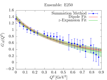
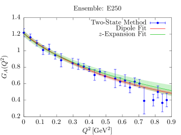
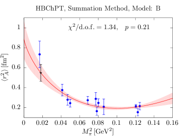
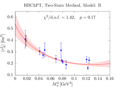
We restrict higher order terms in the expansion from reaching unphysically large values by adding Gaussian priors for all coefficients . Following this procedure we find that a total number of five expansion terms () is sufficient to obtain stable fit results. In order to check for the momentum transfer dependence, we employ several momentum cuts given by . In fig. 1 we show a subset of results of the -expansion fits on the E250 ensemble () with for both the summation method (left panel) with , -value , and the two-state fit (right panel) with , -value . We want to put our main focus on the axial radius extraction so we decide to perform the -expansion fits and the subsequent extrapolation on the normalized effective form factor data for the summation and the two-state extractions corresponding to . In this case the -expansion fits do not include the data points at but constrain the zeroth order coefficient to .
We perform a combined chiral, continuum and infinite-volume extrapolation of our results for obtained from the -expansion fits on every ensemble. With regard to the chiral extrapolation we perform fits which are based on Heavy Baryon Chiral Perturbation Theory (HBChPT) [16] and use the physical pion mass estimate of neglecting electromagnetic and isospin breaking effects [17]. For observable , we employ two different models which differ in the chiral order
| (13) | ||||
| (14) |
Furthermore, we employ two pion-mass cuts given by . In fig. 2 we show the summation method (left column) and the two-state fit (right column) results for both models (top) and (bottom) without including cutoff and finite-volume terms , .
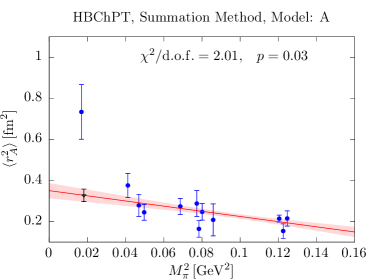
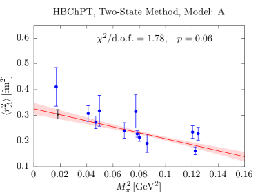
We find the two-state fit results to be more stable with respect to the inclusion of cutoff and finite volume terms. Since we find unexpectedly large () cutoff effects for the summation results we employ a Gaussian prior for restricting the size of the coefficient such that cutoff effects are limited to at most for the coarsest lattice spacing. Additionally, the summation results for fit model show unreasonably large values for the coefficients indicating an artificial behavior of the fit. For this reason we add another prior for the coefficient based on the size of the analytical result for the coefficient in the case of the axial charge [16].
5 Final Results and Outlook
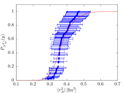
We perform a model average procedure based on the Akaike information criterion [18, 19, 20] associating an AIC-weight to every variation of the extrapolation defined by with and denoting the number of fit parameters and the number of cut data points, respectively. The normalized AIC-weights are used to construct a combined cumulative distribution function (CDF) given by
| (15) |
including all model variations (summation/two-state, model , , , …) represented by normal-distributed random variables with single CDFs denoted by . On the left-hand side of fig. 3 we show the combined CDF defined in eq. (15). We consider the median of the corresponding distribution as the mean of our final result. The statistical and systematic error are obtained from the spread of the percentiles and the scaling behavior of the statistical errors of the model variations. As our final result we quote
| (16) |
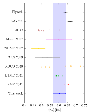
which exhibits a statistical (systematic) error of (). On the right-hand side of fig. 3 we show the comparison of our final result with the experimental values and those obtained by various other lattice collaborations [21, 22, 23, 24, 25, 26]. Within the error interval we are in good agreement with the results of other collaborations and with the experimental world average for the electroproduction.
With regard to further analyses we will increase the number of gauge configurations on the E250 ensemble. Additionally, we plan to add a further gauge ensemble at which will improve the situation concerning the chiral extrapolation. We also plan to analyze with a special focus on excited-state contributions which we assume to play the major role with respect to the systematic uncertainty.
Acknowledgments
This research is partly supported by the Deutsche Forschungsgemeinschaft (DFG, German Research Foundation) through the CRC SFB 1044 (DFG grant HI 2048/1-2 (Project No. 399400745)), and through the Cluster of Excellence (PRISMA+ EXC 2118/1) funded by the DFG (Project ID 39083149). This work is supported by the European Research Council (ERC) under the European Union’s Horizon 2020 research and innovation program through grant agreement No. 771971-SIMDAMA. Calculations for this project were partly performed on the HPC clusters “Clover” and “HIMster2” at the Helmholtz Institute Mainz, and “Mogon 2” at JGU Mainz. Additional computer time has been allocated through projects HMZ21, HMZ23 and HMZ36 on “JUQUEEN” and “JUWELS” at NIC, Jülich. The authors also gratefully acknowledge the Gauss Centre for Supercomputing e.V. (www.gauss-centre.eu) for funding this project by providing computing time on HAZEL HEN at Höchstleistungsrechenzentrum Stuttgart (www.hlrs.de) under project GCS-HQCD. We are grateful to our colleagues within the CLS initiative for sharing gauge field configurations.
References
- [1] Particle Data Group collaboration, Review of Particle Physics, Prog. Theor. Exp. Phys. 2020 (2020) 083C01.
- [2] V. Bernard, L. Elouadrhiri and U.-G. Meißner, Axial structure of the nucleon, J. Phys. G: Nucl. Part. Phys. 28 (2001) R1.
- [3] A.A. Aguilar-Arevalo, C.E. Anderson, A.O. Bazarko, S.J. Brice, B.C. Brown, L. Bugel et al., First measurement of the muon neutrino charged current quasielastic double differential cross section, Phys. Rev. D 81 (2010) 092005.
- [4] A. Bodek, S. Avvakumov, R. Bradford and H. Budd, Vector and axial nucleon form factors: A duality constrained parameterization, Eur. Phys. J. C 53 (2008) 349.
- [5] A.S. Meyer, M. Betancourt, R. Gran and R.J. Hill, Deuterium target data for precision neutrino-nucleus cross sections, Phys. Rev. D 93 (2016) 113015.
- [6] R.J. Hill, P. Kammel, W.J. Marciano and A. Sirlin, Nucleon axial radius and muonic hydrogen—a new analysis and review, Rep. Prog. Phys. 81 (2018) 096301.
- [7] C. Alexandrou, G. Koutsou, J.W. Negele and A. Tsapalis, Nucleon electromagnetic form factors from lattice QCD, Phys. Rev. D 74 (2006) 034508.
- [8] T. Korzec, C. Alexandrou, G. Koutsou, M. Brinet, J. Carbonell, V. Drach et al., Nucleon form factors with dynamical twisted mass fermions, PoS LATTICE 2008 (2009) 139.
- [9] A. Gérardin, T. Harris and H.B. Meyer, Nonperturbative renormalization and -improvement of the nonsinglet vector current with wilson fermions and tree-level symanzik improved gauge action, Phys. Rev. D 99 (2019) 014519.
- [10] P. Korcyl and G.S. Bali, Nonperturbative determination of improvement coefficients using coordinate space correlators in lattice QCD, Phys. Rev. D 95 (2017) 014505.
- [11] M. Dalla Brida, T. Korzec, S. Sint and P. Vilaseca, High precision renormalization of the flavour non-singlet noether currents in lattice QCD with Wilson quarks, Eur. Phys. J. C 79 (2019) 23.
- [12] M. Bruno, D. Djukanovic, G.P. Engel, A. Francis, G. Herdoiza, H. Horch et al., Simulation of QCD with flavors of non-perturbatively improved Wilson fermions, JHEP 2015 (2015) 43.
- [13] M. Bruno, T. Korzec and S. Schaefer, Setting the scale for the CLS flavor ensembles, Phys. Rev. D 95 (2017) 074504.
- [14] D. Djukanovic, T. Harris, G. von Hippel, P.M. Junnarkar, H.B. Meyer, D. Mohler et al., Isovector electromagnetic form factors of the nucleon from lattice QCD and the proton radius puzzle, Phys. Rev. D 103 (2021) 094522.
- [15] R.J. Hill and G. Paz, Model-independent extraction of the proton charge radius from electron scattering, Phys. Rev. D 82 (2010) 113005.
- [16] V. Bernard and U.-G. Meißner, The nucleon axial-vector coupling beyond one loop, Phys. Lett. B 639 (2006) 278.
- [17] S. Aoki, Y. Aoki, D. Bečirević, C. Bernard, T. Blum, G. Colangelo et al., Review of lattice results concerning low-energy particle physics, Eur. Phys. J. C 77 (2017) 112.
- [18] H. Akaike, A new look at the statistical model identification, IEEE Transactions on Automatic Control 19 (1974) 716.
- [19] W.I. Jay and E.T. Neil, Bayesian model averaging for analysis of lattice field theory results, Phys. Rev. D 103 (2021) 114502.
- [20] S. Borsanyi, Z. Fodor, J.N. Guenther, C. Hoelbling, S.D. Katz, L. Lellouch et al., Leading hadronic contribution to the muon magnetic moment from lattice QCD, Nature 593 (2021) 51.
- [21] R. Gupta, Y.-C. Jang, H.-W. Lin, B. Yoon and T. Bhattacharya, Axial-vector form factors of the nucleon from lattice QCD, Phys. Rev. D 96 (2017) 114503.
- [22] S. Capitani, M. Della Morte, D. Djukanovic, G.M. von Hippel, J. Hua, B. Jäger et al., Isovector axial form factors of the nucleon in two-flavor lattice QCD, Int. J. Mod. Phys. A 34 (2019) 1950009.
- [23] E. Shintani, K.-I. Ishikawa, Y. Kuramashi, S. Sasaki and T. Yamazaki, Nucleon form factors and root-mean-square radii on a lattice at the physical point, Phys. Rev. D 99 (2019) 014510.
- [24] G.S. Bali, L. Barca, S. Collins, M. Gruber, M. Löffler, A. Schäfer et al., Nucleon axial structure from lattice QCD, JHEP 2020 (2020) 126.
- [25] S. Park, R. Gupta, B. Yoon, S. Mondal, T. Bhattacharya, Y.-C. Jang et al., Precision nucleon charges and form factors using 2+1-flavor lattice QCD, 2103.05599.
- [26] C. Alexandrou, S. Bacchio, M. Constantinou, P. Dimopoulos, J. Finkenrath, K. Hadjiyiannakou et al., Nucleon axial and pseudoscalar form factors from lattice QCD at the physical point, Phys. Rev. D 103 (2021) 034509.