Scheduling and dimensioning of heterogeneous energy stores, with applications to future GB storage needs

Abstract

Future “net-zero” electricity systems in which all or most generation is renewable may require very high volumes of storage, provided jointly by a number of heterogeneous technologies, in order to manage the associated variability in the generation-demand balance. We consider the problems of scheduling and dimensioning such storage. We develop a value-function based approach to optimal scheduling, and show that, to a good approximation, the problem to be solved at each successive point in time reduces to a linear programme with a particularly simple solution. We show that approximately optimal scheduling may be achieved without the need for a running forecast of the future generation-demand balance. We examine the applicability of the above theory to future GB storage needs, and discuss how it may be used to enable the most economic dimensioning of such storage, with possible savings of tens of billions of pounds, relative to the use of a single technology.

Keywords: energy storage; economics; optimal scheduling.

1 Introduction

Future electricity systems in which all or most generation is renewable, and hence highly variable, may require extremely high volumes of storage in order to manage this variability and to ensure that demand may always be met—see [24, 16, 2, 18], and especially [22], for an assessment of likely future needs and costs in Great Britain, where, under a future “net-zero” carbon emissions strategy, capital costs of storage may run into many tens, or even hundreds, of billions of pounds. For the reasons we explain below, a mixture of storage technologies is likely to be required. The problems considered in the present paper are those of the scheduling and dimensioning of such storage, with the objective of meeting energy demand to a required reliability standard as economically as possible. These problems are considered from a societal viewpoint, which generally coincides with that of the electricity system operator. This is in contrast the viewpoint of a storage provider seeking to maximise profits (see [21, 4, 5, 10, 17, 26] and the references therein). Insofar as the societal problem of managing energy storage is considered in the existing literature, this is mostly in the context of short-term storage used to cover occasional periods of generation shortfall, with sufficient time for recharging between such periods (see, e.g. [14, 11, 20, 29]). The scheduling problems we consider in this paper are nontrivial in that, if storage is not managed properly, then it is likely that there will frequently arise the situation in which there is sufficient energy in storage to meet demand but it is located in too few stores for it to be possible to serve it at the required rate. The need for a solution of these scheduling problems is highlighted by the forthcoming Royal Society report [22] on long-term energy storage in GB. The present paper aims to supply the necessary mathematics for that, and to illustrate its application in the context of future GB storage needs.

In a large system, such as that of Great Britain, which we consider further in Section 4, the processes of demand and of renewable generation vary on multiple timescales: on a timescale measured in hours there is diurnal variation in demand and in solar generation; on a timescale of days and weeks there is weather-related variation in demand and in most forms of renewable generation, and there is further demand variation due to weekends and holiday periods; on longer timescales there is seasonal variation in both demand and renewable generation which may extend to major differences between successive years (see [2, 18] for more details). In GB, for example, it is particularly the case that some years are significantly windier than others (see [23]), necessitating volumes of storage of the order of tens of terawatt-hours within a future net-zero scenario—see Section 4 and [19] for similar results in the US context.

Variation in the generation-demand balance may be managed by a number of different storage technologies. These vary greatly in their costs per unit of capacity and per unit of power (the maximum rate at which they may be charged or discharged), and further in their (round-trip) efficiencies (energy output as a fraction of energy input). In consequence, different storage technologies are typically appropriate to managing variation on these different timescales—see [2, 18, 22] for detailed comparisons and analysis in the GB context, and also the recent report [12] (especially Figure 1.6) for a discussion of differing technology costs and their implications. We further explore these issues in Section 4.

It thus seems likely that, in the management of such future electricity systems, there will be a need for a mix of storage technologies. This will be such that most of the required storage capacity will be provided by those technologies such as chemical storage, which are able to provide this capacity economically, while a high proportion of the power requirements will be met by technologies such as batteries or advanced (adiabatic) compressed air energy storage (ACAES) with much lower input-output costs and higher efficiencies. (Although there is considerable uncertainty in future costs, we show that, for the GB examples of Section 4 and on the basis of those costs given by [12], Figure 1.6, or by [2, 18], it is likely that the use of an appropriate mixture of storage technologies would result in cost savings of the order of many billions of pounds, compared with the use of the most economical single technology. In particular, focusing on those technologies which minimise capacity costs alone leads to technology mixes which, when power costs are added, are extremely expensive—again see [18].) There now arise the questions of how such storage may be economically dimensioned, and of how it may be managed—the ability to answer the former question depending on having a sufficiently good understanding of the answer to the latter. The problem of managing, or scheduling, any given set of stores is that of deciding by how much each individual store should be charged or discharged at each successive point in time in order to best manage the generation-demand (im)balance—usually with the objective of minimising total unmet demand, or unserved energy, over some given period of time. In this context, usually those stores corresponding to any given technology may be treated as a single store provided their capacity-to-power ratios are approximately equal (see Section 2). However, the scheduling problem is a real-time problem, and in deciding which storage technology to prioritise at any given point in time, it is difficult to attempt to classify the current state of the generation-demand balance as representing short, medium, or long-term variation. Within the existing literature and in assessing likely GB storage needs, [18] use a heuristic algorithm to attempt such a decomposition, while [2] use a filtering approach to choose between medium- and long-term storage. (Neither of these approaches allows for cross-charging—see Section 2.) The present paper formulates the scheduling problem as one in mathematical optimisation theory in order to derive policies in which cooperation between stores happens automatically when this is beneficial, thereby enabling given generation-demand balance processes to be managed by storage systems which are considerably more compactly dimensioned in their power requirements in particular (see also [22]).

Section 2 of the paper defines the relevant mathematical model for the management of multiple stores. This incorporates capacity and rate (power) constraints, together with round-trip efficiencies, and allows for entirely general scheduling policies. Section 3 develops the relevant mathematics for the identification of optimal policies, when the objective is the minimisation of cumulative unserved energy to each successive point in time. We show that it is sufficient to consider policies that are greedy in an extended sense defined there. We further show that, at each successive point in time, the scheduling problem may be characterised as that of maximising a value function defined on the space of possible energy levels of the stores, and that, under appropriate conditions, the optimisation problem to be solved at that time is approximately a linear programme which has a simple, non-iterative, solution. We give conditions under which it is possible to find optimal policies, exact or approximate, from within the class of non-anticipatory policies, i.e. those which do not require real-time forecasting of the generation-demand balance. Section 4 considers an extended application to future GB energy storage needs, which, under the conditions considered, aims to be as realistic as possible. The aims here are both to demonstrate the applicability of the present theory, and further to show how one might reasonably go about solving the practical problems of identifying, dimensioning and managing future storage needs. We demonstrate the general success, and occasional limitations, of non-anticipatory policies as defined above. We indicate briefly how the analysis might be extended to include network constraints, if desired, although we also indicate why these are less significant in the context of dimensioning long-term storage. The concluding Section 5 considers some practical implications of the preceding results.

2 Model

We study the management over (discrete) time of a set $S$ of stores, where each store $i\in S$ is characterised by four parameters $(E_{i},Q_{i},P_{i},\eta_{i})$ as described below. For each store $i\in S$, we let $s_{i}(0)$ be the initial level of energy in store $i$ and $s_{i}(t)$ be the level of energy in store $i$ at (the end of) each subsequent time $t\geq 1$. Without loss of generality and for simplicity of presentation of the necessary theory, we make the convention that the level of energy in each store at any time is measured by that volume of energy that it may ultimately supply, so that, within the model, any (round-trip) inefficiency of the store is accounted for at the input stage. While accounting for such inefficiency is essential to our modelling and results, we assume that energy, once stored, is not further subject to significant time-dependent leakage. However, the theory of the present paper would require only minor adjustments to incorporate such time-dependent leakage.

The successive levels of energy in each store $i$ satisfy the recursion

$$s_{i}(t)=s_{i}(t-1)+r_{i}(t),\qquad t\geq 1,$$ (1)

where $r_{i}(t)$ is the rate (positive or negative) at which energy is added to the store $i$ at the time $t$. Each store $i\in S$ is subject to capacity constraints

$$0\leq s_{i}(t)\leq E_{i},\qquad t\geq 0,$$ (2)

so that $E_{i}>0$ is the capacity of store $i$ (again measured by the volume of energy it is capable of serving) and rate constraints

$$-P_{i}\leq r_{i}(t)\leq\eta_{i}Q_{i},\qquad t\geq 1.$$ (3)

Here $P_{i}>0$ is the (maximum) output rate of the store $i$, while $Q_{i}>0$ is the (maximum) rate at which externally available energy may be used for input to the store, with the resulting rate at which the store fills being reduced by the round-trip efficiency $\eta_{i}$ of the store, where $0<\eta_{i}\leq 1$. Given the vector $s(0)=(s_{i}(0),\,i\in S)$ of the initial levels of energy in the stores, a policy for the subsequent management of the stores is a specification of the vector of rates $r(t)=(r_{i}(t),\,i\in S)$, for all times $t\geq 1$; equivalently, from (1), it is a specification of the vector of store levels $s(t)=(s_{i}(t),\,i\in S)$, for all times $t\geq 1$. (The question of how a policy may be chosen in real-time applications is considered in Section 3.)

The stores are used to manage as far as possible a residual energy process $(\mathit{re}(t),\,t\geq 1)$, where, for each time $t$, a positive value of $\mathit{re}(t)$ corresponds to surplus energy available for charging the stores, subject to losses due to inefficiency, and a negative value of $\mathit{re}(t)$ corresponds to energy demand to be met as far as possible from the stores. In applications, the residual energy $\mathit{re}(t)$ is usually the surplus of generation over demand at each successive time $t$. For any time $t$, given the vector of rates $r(t)=(r_{i}(t),\,i\in S)$, define the imbalance $u(t)$ by

$$u(t)=\mathit{re}(t)-\sum_{i\colon r_{i}(t)<0}r_{i}(t)-\sum_{i\colon r_{i}(t)\geq 0}r_{i}(t)/\eta_{i}.$$ (4)

We shall require also that that the policy defined by the rate vectors $r(t)$, $t\geq 1$, is such that, at each successive time $t$,

$$\mathit{re}(t)\geq 0\quad\Rightarrow\quad u(t)\geq 0,$$ (5)

so that, at any time $t$ when there is an energy surplus, the net energy input into the stores, before losses due to round-trip inefficiency, cannot exceed that surplus; the quantity $u(t)$ is then the spilled energy at time $t$. Similarly, we shall require that

$$\mathit{re}(t)\leq 0\quad\Rightarrow\quad u(t)\leq 0,$$ (6)

so that, at any time $t$ when there is an energy shortfall, i.e. a positive net energy demand to be met from stores, the net energy output of the the stores does not exceed that demand; under the constraint (6), the quantity $-u(t)$ is then the unserved energy at time $t$. (It is not difficult to see that, under any reasonable objective for the use of the stores to manage the residual energy process—including the minimisation of total unserved energy as discussed below—there is nothing to be gained by overserving energy at times $t$ such that $\mathit{re}(t)\leq 0$.) We shall say that a policy is feasible for the management of the stores if, for each $t\geq 1$, that policy satisfies the above relations (1)–(6).

For any feasible policy, define the total unserved energy $\mathit{ue}(t)$ to any time $t$ to be the sum of the unserved energies at those times $t^{\prime}\leq t$ such that $\mathit{re}(t^{\prime})\leq 0$, i.e.

$$\mathit{ue}(t)=-\sum_{t^{\prime}\leq t:\,\mathit{re}(t^{\prime})\leq 0}u(t^{\prime})=\sum_{t^{\prime}\leq t}\max(0,-u(t^{\prime})),$$ (7)

where the second equality above follows from (5) and (6). Our objective is to determine a feasible policy for the management of the stores so as to minimise the total unserved energy over (some specified period of) time. It is possible that, at any time $t$, some store $i$ may be charging ($r_{i}(t)>0$) while some other store $j$ is simultaneously discharging ($r_{j}(t)<0$). We refer to this as cross-charging—although the model does not of course identify the routes taken by individual electrons. Although, in the presence of storage inefficiencies, cross-charging is wasteful of energy, it is nevertheless occasionally effective in enabling a better distribution of energy among stores and avoiding the situation in which energy may not be served at a sufficient rate because one or more stores are empty.

We make also the following observation. Suppose that some subset $S^{\prime}$ of the set of stores $S$ is such that the stores $i\in S^{\prime}$ have common efficiencies $\eta_{i}$ and common capacity-to-power ratios $E_{i}/P_{i}$ and $E_{i}/Q_{i}$. Then it is clear that these stores may be optimally managed by keeping the fractional storage levels $s_{i}(t)/E_{i}$ equal across $i\in S^{\prime}$ and over all times $t$, so that the stores in $S^{\prime}$ effectively behave as a single large store with total capacity $\sum_{i\in S^{\prime}}E_{i}$ and total input and output rates $\sum_{i\in S^{\prime}}Q_{i}$ and $\sum_{i\in S^{\prime}}P_{i}$ respectively. This is relevant when, as in the application of Section 4, we wish to consider the scheduling and dimensioning of different storage technologies in order to obtain an optimal mix of the latter. Then, for this purpose, it is reasonable to treat—to a good approximation—the storage to be provided by any one technology as constituting a single large store.

3 Nature of optimal policies

We continue to take as our objective the minimisation of total unserved energy over some given period of time. We characterise desirable properties of policies for the management storage, and show how at least approximately optimal policies may be determined.

In applications, the residual energy process to be managed is not generally known in advance (so ruling out, e.g., the use of straightforward linear programming approaches) and policies must be chosen dynamically in response to evolving information about that process. Within our discrete-time setting, the information available for decision-making at any time $t$ will generally consist of the vector of store levels $s(t-1)=(s_{i}(t-1),\,i\in S)$ at the end of the preceding time period (equivalently the start of the time period $t$) together with the current value $\mathit{re}(t)$ of the residual energy process at the time $t$. However, this information may be supplemented by some, necessarily probabilistic, prediction (however obtained) of the evolution of the residual energy process subsequent to time $t$. We shall be particularly interested in identifying conditions under which it is sufficient to consider (feasible) policies in which the decision to be made at any time $t$, i.e. the choice of rates vector $r(t)$, depends only on $s(t-1)$ and $\mathit{re}(t)$, thereby avoiding the need for real-time prediction of the future residual energy process. Such policies are usually referred to as non-anticipatory, or without foresight.

Section 3.1 below defines greedy policies and shows that it is sufficient to consider such policies. Section 3.2 discusses conditions under which a (greedy) optimal, or approximately optimal, policy may be found from within the class of non-anticipatory policies. Section 3.3 shows that the immediate optimisation problem to be solved at each successive time $t$ may be characterised as that of maximising a value function defined on the space of possible store (energy) levels, and identifies conditions under which this latter problem is approximately a linear programme—with a particularly simple, non-iterative, solution.

3.1 Greedy policies

We define a greedy policy to be a feasible policy in which, at each successive time $t\geq 1$, and given the levels $s(t-1)$ of the stores at the end of the preceding time period,

• if the residual energy $\mathit{re}(t)\geq 0$, i.e. there is energy available for charging the stores at time $t$, then there is no possibility to increase any of the rates $r_{i}(t)$, $i\in S$ (without decreasing any of the others), and so further charge the stores, while keeping the policy feasible; equivalently, we require that if the spilled energy $u(t)>0$ (where $u(t)$ is defined by (4)), then $r_{i}(t)=\min(E_{i}-s_{i}(t-1),\,\eta_{i}Q_{i})$ for all $i\in S$; thus the spilled energy $u(t)$ at time $t$ is minimised.

• if the residual energy $\mathit{re}(t)<0$, i.e. there is net energy demand at time $t$, then there is no possibility to decrease any of the rates $r_{i}(t)$, $i\in S$ (without increasing any of the others), and so further serve demand, while keeping the policy feasible; equivalently, we require that if the unserved energy $-u(t)>0$, then $r_{i}(t)=-\min(s_{i}(t-1),\,P_{i})$ for all $i\in S$; thus the unserved energy $-u(t)$ at time $t$ is minimised.

Note that if $\mathit{re}(t)=0$ at time $t$, then, for a feasible policy, it is necessarily the case, from (5) and (6), that the imbalance $u(t)=0$.

Proposition 1 and its corollary below generalise a result of [7] (in that case for a single store which can only discharge) to show that, under the objective of minimising the total unserved energy, it is sufficient to consider greedy policies.

Proposition 1.

Any feasible policy may be modified to be greedy while remaining feasible and while continuing to serve as least as much energy to each successive time $t$. Further, if the original policy is non-anticipatory, the modified policy may be taken to be non-anticipatory.

Proposition 1 is intuitively appealing: at those times $t$ such that $\mathit{re}(t)\geq 0$, there is no point in withholding energy which might be used for charging any store, since the only possible “benefit” of doing so would be to allow further energy—not exceeding the amount originally withheld—to be placed in that store at a later time. Similarly, at those times $t$ such that $\mathit{re}(t)<0$, there is no point in withholding energy in any store which might be used to reduce unserved energy, since the only possible “benefit” of doing so would be to allow additional demand—not exceeding that originally withheld by that store—to be met by that store at a later time. A formal proof of Proposition 1 is given in the Appendix. Note that greedy policies may involve cross-charging (see Section 2). Proposition 1 has the following corollary.

Corollary 1.

Suppose that the objective is the minimisation of unserved energy over some given period of time. Then there is an optimal policy which is greedy. Further, within the class of non-anticipatory policies there is a greedy policy which is optimal within this class.

We remark that under objectives other than the minimisation of total unserved energy, optimal policies may fail to be greedy. For example, if unserved energy were costed nonlinearly, or differently at different times, then at certain times it might be better to retain stored for more profitable use at later times—see, for example, [3].

3.2 Non-anticipatory policies

There are various conditions (see below) under which the optimal policy may be taken to be not only greedy (see Proposition 1) but also non-anticipatory as defined above. We are therefore led to consider whether it is sufficient in applications to consider non-anticipatory policies—at least to obtain results which are at least approximately optimal, and to design and dimension storage configurations. Two such non-anticipatory policies which work well under different circumstances are:

• The greedy greatest-discharge-duration-first (GGDDF) policy (see [13, 8, 3, 28]) is a storage discharge policy for managing a given residual energy process which is negative (i.e. there is positive energy demand) over a given period of time, with the aim of minimising total unserved energy. It is defined by the requirement that, at each time $t$, stores are prioritised for discharging in order of their residual discharge durations, where the residual discharge duration of a store $i$ at any time is defined as the energy in that store at the start of time divided by its maximum discharge rate $P_{i}$. This non-anticipatory policy is designed to cope with rate constraints and to avoid as far as possible the situation in which there are times at which there is sufficient total stored energy, but this is located in too few stores. It is optimal among policies which do not involve cross-charging, and more generally under the conditions discussed in [28]. As also discussed there, it may be extended to situations where the residual energy process is both positive and negative.

• The greatest-round-trip-efficiency first (GRTEF) policy is a greedy policy which is designed to cope with round-trip inefficiency: stores are both charged and discharged—in each case to the maximum feasible extent—in decreasing order of their efficiencies and no cross-charging takes place. In the absence of output rate constraints, the GRTEF policy may be shown to be optimal: straightforward coupling arguments, similar to those used to prove Proposition 1, show that, amongst greedy policies, the GRTEF policy maximises the total stored energy $\sum_{i\in S}s_{i}(t)$ at any time, so that energy which may be served under any other policy may be served under this policy.

In practice, a reasonable and robust policy might be to use the GRTEF policy whenever no store is close to empty, and otherwise to switch to the GGDDF policy. However, there is a need to find the right balance between these two policies, and also to allow for the possibility of cross-charging where this might be beneficial. We therefore look more generally at non-anticipatory policies. The choice of such policies is informed both by some considerations from dynamic programming theory and by the observations above.

3.3 Value functions

Standard dynamic programming theory (see, e.g. [1]) shows that, at any time $t$, given a stochastic description of the future evolution of the residual energy process, an optimal decision at that time may be obtained through the computation of a value function $V^{t}(s)$ defined on the set of possible states $s=(s_{i},\,i\in S)$ of the stores, where each $s_{i}=s_{i}(t-1)$ is the level of energy in store $i\in S$ at the start of time $t$. The quantity $V^{t}(s)$ may be interpreted as the future value of having the energy levels of the stores in state $s$ at time $t$, relative to their being instead in some other reference state, e.g. state $0$, where value is the negative of cost as measured by expected future unserved energy. Then the optimal decision at any time $t$ is that which maximises the value of the resulting state, less the cost of any energy unserved at time $t$. In the present problem, such a stochastic description is generally unavailable. However, the value function might reasonably be estimated from a sufficiently long residual energy data series—typically of at least several years duration—especially if one is able to assume (approximate) time-homogeneity of the above stochastic description. The latter assumption essentially corresponds, over sufficiently long time periods, to the use of a value function $V^{t}(s)=V(s)$ which is independent of time $t$ and to the use of a non-anticipatory scheduling policy (however, see below).

As previously indicated, we make the convention that the state $s_{i}$ of each store $i$ denotes the amount of energy which it is able to serve—so that (in)efficiency losses are accounted for at the input stage. At any time $t$, and given a stochastic description as above, the value function $V^{t}(s)$ may be computed in terms of absorption probabilities (see, e.g. [6]). For each $t$, let $v^{t}_{i}(s)$ be the partial derivative of the value function $V^{t}(s)$ with respect to variation of the level $s_{i}$ of each store $i\in S$. Standard probabilistic coupling arguments (which we do not give in detail since they are not formally required here) show that, for each $i\in S$, $v^{t}_{i}(s)$ lies between $0$ and $1$ and is decreasing is $s_{i}$. (For example, the positivity of $v^{t}_{i}(s)$ is simply the monotonicity property that one can never be worse off by having more stored energy—see Section 2). We assume that changes in store energy levels are sufficiently small over each single time step $t$ that changes to the value function may be measured using the above partial derivatives. Then the above problem of scheduling the charging or discharging of the stores over the time step $t$ becomes that of choosing feasible rates $r(t)=(r_{i}(t),\,i\in S)$ so as to maximise

$$\sum_{i\in S}v^{t}_{i}(s)r_{i}(t)-\max(0,-u(t)),$$ (8)

where $s_{i}=s_{i}(t-1)$ is again the level of each store $i\in S$ at the end of the preceding time step $t-1$, and where the second term in (8)) is the unserved energy at time $t$ (see Section 2). Thus, under the above linearisation, the scheduling problem at each time $t$ becomes a linear programme.

When, at (the start of) any time $t$, the state of the stores is given by $s=s(t-1)$, we shall say that any store $i\in S$ has charging priority over any store $j\in S$ if $\eta_{i}v^{t}_{i}(s)>\eta_{j}v^{t}_{j}(s)$, and that any store $i\in S$ has discharging priority over any store $j\in S$ if $v^{t}_{i}(s)<v^{t}_{j}(s)$. Proposition 2 below is again intuitively appealing; we give a formal proof in the Appendix.

Proposition 2.

When the objective is the minimisation of total unserved energy over some given period of time, then, under the above linearisation, at each time $t$ and with $s=s(t-1)$, the optimal charging, discharging and cross-charging decisions are given by the following procedure:

• when charging, i.e. if $\mathit{re}(t)\geq 0$, charge the stores in order of their charging priority, charging each successive store as far as permitted (the minimum of its input rate and its residual capacity) until the energy available for charging at time $t$ is used as far as possible—any remaining energy being spilled;

• when discharging, i.e. if $\mathit{re}(t)<0$, discharge the stores in order of their discharging priority, discharging each successive store as far as permitted (the minimum of its output rate and its available stored energy) until the demand at time $t$ is met as fully as possible—any remaining demand being unserved energy;

• subsequent to either of the above, choose pairs of stores $(i,j)$ in succession by, at each successive stage, selecting store $i$ to be the store with the highest discharging priority which is still able to supply energy at the time $t$ and selecting store $j$ to be the store with the highest charging priority which is still able to accept energy at the time $t$; for each such successive pair $(i,j)$, provided that

  $$v^{t}_{i}(s)<\eta_{j}v^{t}_{j}(s),$$ (9)

  cross-charge as much energy as possible from store $i$ to store $j$. Note that the above priorities are such that this process necessarily terminates on the first occasion such that the condition (9) fails to be satisfied, and further that no cross-charging can occur when $\mathit{re}(t)\geq 0$ and there is spilled energy, or when $\mathit{re}(t)<0$ and there is unserved energy.

The pairing of stores for cross-charging in the above procedure is entirely notional, and what is important is the policy thus defined. However, when efficiencies are low, cross-charging occurs infrequently.

In the examples of Section 4, we consider time-homogeneous value function derivatives of the form

$$v^{t}_{i}(s)=\exp(-\lambda_{i}s_{i}/P_{i}),\quad i\in S,$$ (10)

essentially corresponding, as above, to the use of non-anticipatory scheduling algorithms. (However, data limitations—see the analysis of Section 4—mean that we use a single, extremely long, residual energy dataset of 324,360 hourly observations both to estimate the parameters $\lambda_{i}$ and to examine the effectiveness of the resulting policies. Hence, the resulting scheduling algorithms might be regarded as having, at each successive point in time, some very mild anticipation of the future evolution of the residual energy process. Within the present exploratory analysis this approach seems reasonable.)

The expression (10) is an approximation, both in its assumption that, for each $i\in S$, the partial derivative $v^{t}_{i}(s)$ depends only on the state $s_{i}$ of store $i$, and in the assumed functional form of the dependence of $v^{t}_{i}(s)$ on $s_{i}$. The former assumption is equivalent to taking the value function as a sum of separate contributions from each store (a reasonable first approximation), while probabilistic large deviations theory [6] suggests that, under somewhat idealised conditions, when the mean residual energy is positive, the functions $v^{t}_{i}(s)$ do decay exponentially. However, we primarily justify the use of the relation (10) in part by the arguments below, and in part by its practical effectiveness—see the examples of Section 4. Recall that what are important are the induced decisions, as described above, on the storage configuration space. In particular, when the stores are under pressure and hence discharging, it follows from the definition of discharging priority above that it is only the ratios of the parameters $\lambda_{i}$ which matter, except only for determining the extent to which cross-charging should take place. Taking $\lambda_{i}=\lambda$ for all $i$ and for some $\lambda$ defines a policy which, when discharging, corresponds to the use of the GGDDF policy, supplemented by a degree of cross-charging which depends on the absolute value of the parameter $\lambda$. The ability to further adjust the relative values of the parameters $\lambda_{i}$ between stores allows further tuning to reflect their relative efficiencies; in particular, for a given volume of stored energy, increasing the efficiency of a given store $i\in S$ increases the desirability of having that energy stored in other stores and reserving more of the capacity of store $i$ for future use—something which can be effected by increasing the parameter $\lambda_{i}$.

4 Application to GB energy storage needs

In this section we give an extended example of the application of the preceding theory to the problem of dimensioning and scheduling future GB energy storage needs within a net-zero environment. Our primary aim is to illustrate the practical applicability of the theory. We also aim to show how, given also cost data, it might be used to assist in storage dimensioning. We are further concerned with the extent to which it is sufficient to consider non-anticipatory scheduling policies.

A detailed description of the dimensioning problem in the GB context, together with details of all our storage, demand and renewable generation data, including storage costs, is given by [18]—work prepared in support of the Royal Society working party on future GB energy storage. (That paper uses a rather heuristic scheduling algorithm, which occasionally leads to very high total power requirements.) Additional discussion is given in the Royal Society report itself [22]. We consider here a GB 2050 net-zero scenario, also considered in [18, 22]. In this scenario heating and transport are decarbonised, in line with the UK’s 2050 net-zero commitment, thereby approximately doubling current electricity demand to 600 TWh per year (see [25]), and all electricity generation is renewable and provided by a mixture of 80% wind and 20% solar generation. (In particular, it is assumed that there is no fossil-fuel based generation, even with carbon-capture-and-storage.) It is further assumed that there is a 30% level of generation overcapacity—corresponding to total renewable generation of 780 TWh per year on average. The above wind-solar mix and level of generation overcapacity are those used in [18, 22], and are approximately optimal on the basis of the generation and cost data considered there. We also consider, more briefly, the effect on storage dimensioning of a reduced level of overcapacity of 25%. However, on the basis of the costs given by [18], the 5% reduction in generation overcapacity (30 TWh) saves $15 bn in generation costs, with the consequence that, in all the examples below, the 30% level of overcapacity is here more economic. The lower level of overcapacity is included for comparison purposes.

In the application of this section, we depart from our earlier convention (made for mathematical simplicity) of notionally accounting for all round-trip inefficiency at the input stage. We instead split the efficiency $\eta_{i}$ of any store $i$ by taking both the input and output efficiencies to be given by $\eta_{i}^{0.5}$. This revised convention increases both the notional volumes of energy within any store $i$ and the notional capacity of the store $i$ by a factor $\eta_{i}^{-0.5}$. This is in line with most of the applied literature on energy storage needs and makes our storage capacities below directly comparable with those given elsewhere.

Generation and demand data.

We use a dataset consisting of 37 years of hourly “observations” of wind generation, solar generation and demand. The wind and solar generation data are both based on the 37-year (1980–2016) reanalysis weather data of [23] together with assumed installations of wind and solar farms distributed across GB and appropriate to the above scenario, and with 80% wind and 20% solar generation as above. The derived generation data are scaled so as to provide on average the required level of generation overcapacity relative to the modelled demand. The demand data are taken from a year-long hourly demand profile again corresponding to the above 2050 scenario and in which there is 600 TWh of total demand; this profile was prepared by Imperial College for the UK Committee on Climate Change [25]. As in [18, 22] this year-long set of hourly demand data has been recycled to provide a 37-year trace to match the generation data. (This is reasonable here as the between-years variability which may present challenges to storage dimensioning and scheduling is likely to arise primarily from the between-years variability in renewable generation. However, see also [9]). More details and some analysis of the above data are given in [18]. From these data we thus obtain a 37-year hourly residual energy (generation less demand) process to be managed by storage. For the chosen base level of 30% generation overcapacity, Figure 1 shows a histogram and autocorrelation function of the hourly residual energy process. The large variation in the residual energy process is to be compared with the mean demand of 68.6 GW.

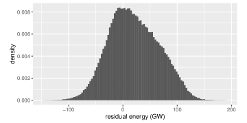
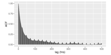
Figure 1: Histogram and autocorrelation function of hourly residual energy (30% overcapacity).

Some level of generation overcapacity is required, both to account for losses due to inefficiencies in storage, and to keep the required volume of storage within reasonable bounds. As the level of generation overcapacity increases, storage requirements (specifically, capacities and input rates) decrease. The consequent decrease in storage costs must be balanced against the increase in the cost of generation. In our examples below, the considered levels of generation overcapacity are 30% and 25%. However, it is useful to consider briefly the volume of storage required to manage more general levels of overcapacity. In particular, for a single store with given efficiency and without input or output power constraints, there is a minimum store size and a minimum initial store energy level such that the store can completely manage the above residual energy process (i.e. with no unmet demand). Figure 2 plots, for various levels of store efficiency and on the basis of our assumed 80%-20% wind-solar mix, this minimum store size against the assumed level of overcapacity in the above residual energy process.

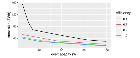
Figure 2: Dependence of minimal store size on level of generation overcapacity for various (round-trip) efficiencies.

Storage data and costs.

As discussed in Section 1 and in [18], we consider three types of storage with associated efficiencies:

• the short store is intended primarily for the management of diurnal and other short-term variation, and has a low capacity requirement (see below); it is assumed that it can therefore use a technology such as Li-ion battery storage with a high efficiency, which we here take to be $0.9$;

• the medium store is intended primarily for the management of variation on a timescale of days and weeks, this variation resulting from weather-related variations in generation and demand; it has very substantial capacity requirements and may require a technology such as ACAES which has a lower efficiency, which we here take to be $0.7$;

• the long store is intended for the management of seasonal and between-years variation (see Section 1); it has an very high capacity requirement, and a power requirement which—on account of potentially high input/output costs—it is desirable to keep relatively modest; it requires a technology, such as hydrogen or similar chemical storage, which currently has a low efficiency, which we here take to be $0.4$.

We use storage costs from [18], Table 3, and given in Table 1 below (with storage capacity measured according to to the convention of this section with regard to accounting for inefficiency). These costs are based on various recent studies as reported in the above paper and are estimates of likely future storage costs in 2040 if the storage technologies are applied on a large scale—current costs are considerably higher. For Li-ion batteries, the maximum input and output rates are constrained to be the same, so that power costs may be associated with input power. However, there is huge uncertainty as to future storage costs and so the examples below are not to be read as providing recommendations about competing storage technologies.

	capacity	output power	input power
	($ per KWh)	($ per KW)	($ per KW)
long (hydrogen)	0.8	429	858
medium (ACAES)	9.0	200	200
short (Li-ion)	100.0	0	180

Table 1: Storage costs (US dollars) used for examples.

Unit capacity costs decrease dramatically (by some orders of magnitude) as we move from the short, to the medium, to the long store, while unit power (rate) costs vary, again considerably, in the opposite direction. The aim in dimensioning and scheduling storage must therefore be to arrive at a position in which the long store is meeting most of the total capacity requirement, while as much as is reasonably possible of the total power requirement is being met by the medium and short stores.

We treat GB as a single geographical node, ignoring network constraints. This is in line with most current studies of GB long-term storage needs, see, e.g. [2, 18, 22], and in line with the annual Electricity Capacity Reports produced by the GB system operator [15]. As at present, future network constraints are unlikely to be continuously binding over periods of time in excess of a few hours, or a day or two at most, and are primarily likely to affect and to increase short-term storage requirements. (The effect of such constraints on the model of the present paper would be to add further linear constraints on the input and output rates of the stores. The general theory given in the preceding sections would continue to be applicable.)

We take the reliability standard to be given by 24 GWh per year unserved energy and optimise scheduling and dimensioning subject to to constraint that this standard is met. This results in an average number of hours per year in which there is unserved energy which is roughly in line with the current GB standard of a maximum of 3 such hours per year. However, modest variation of the chosen reliability standard makes very little difference to our conclusions.

Example 1 below considers a single store. In the remaining examples we schedule storage using time-homogeneous value function derivatives $v_{i}(s)$ given by (10) (with $s$ defined as there to be the volume of stored energy which may be output). Thus, as previously discussed, the scheduling is almost completely non-anticipatory. We consider also the optimality of the scheduling algorithms used.

We take the stores to be initially full. However, in all our examples, stores fill rapidly regardless of their initial energy levels, and these levels are in general independent of their initial values by the end of the first year of the 37-year period considered.

Example 1.

Single long (hydrogen) store with efficiency 0.4. We first consider the management of the residual energy process by a single store, optimally dimensioned with respect to cost. If a single store is to be used, then, of the technologies considered here and on the basis of the present, as yet very uncertain, costs, a hydrogen store is the only economic possibility—see also [18, 22]

The unserved energy is clearly a decreasing function of each of the store capacity $E$, the maximum input power $Q$ and the maximum output power $P$. For any given value of $P$, we may thus easily minimise the overall cost over $(E,Q)$. It then turns out—unsurprisingly given the stringent reliability standard—that the overall cost is here minimised by taking $P$ to be the minimum possible value (115.9 GW or 116.6 GW at 30% or 25% generation overcapacity) such that the given reliability standard of 24 GWh per year is satisfied. Table 2 shows the optimal storage dimensions and associated costs for both the levels of generation overcapacity considered in these examples.

30% generation overcapacity                                                                            
capacity output power input power total size 120.4 TWh 115.9 GW 80.0 GW cost ($ bn) 96.3 49.7 68.6 214.7

25% generation overcapacity                                                                            
capacity output power input power total size 167.9 TWh 116.6 GW 85.3 GW cost ($ bn) 134.3 50.0 73.2 257.5

Table 2: Single long (hydrogen) store: dimensions and costs.

These store capacities are larger than those suggested by Figure 2, where the maximum store input powers $Q$ were unconstrained: on the basis of the present costs, it is in each case more economic to reduce $Q$ at the expense of allowing the store capacity $E$ to increase.

The total cost of storage required to manage 25% generation overcapacity is $42.8 bn greater than the corresponding cost at 30% overcapacity—making the 30% level of overcapacity more economic on the basis of the storage and generation costs discussed above.

Figure 3 plots cumulative unserved energy against time for each of the two levels of generation overcapacity. These two processes are here essentially identical. In each case, the store never completely empties and so unserved energy occurs only at those times at which the output power $P$ of the store is insufficient to serve demand.

Figure 3: Example 1: single long (hydrogen) store: cumulative unserved energy.

Figure 4 shows the corresponding processes formed by the successive energy levels within the store. A substantial fraction of the store capacity is needed solely to manage the single period of large shortfall in the residual energy process occurring at around 275,000 hours into the 37-yr (324,360 hour) period studied. This underlines the importance of using a residual energy time-series which is sufficiently long to capture those events such as sustained wind droughts which only occur perhaps once every few decades—see also [22].

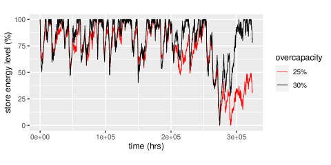
Figure 4: Example 1: single long (hydrogen) store: successive store energy levels.

Example 2.

Long (hydrogen) store with efficiency 0.4 plus medium (ACAES) store with efficiency 0.7. In this example we show that, again on the basis of the cost data used here and the considered levels of generation overcapacity, extremely large savings (of the order of tens of billions of dollars) are to be made by the use of a suitable mixture of storage technologies.

We choose medium (ACAES) store dimensions as below: for both levels of generation overcapacity, some numerical experimentation shows these to be at least close to optimal with respect to overall cost minimisation. Then, given these medium store dimensions, and subject to the given reliability standard, the long (hydrogen) store may be optimally dimensioned—given the use of the value-function based scheduling algorithm, and again to a very good approximation—as previously. Table 3 shows the optimal storage dimensions and associated costs, again for both 30% and 25% generation overcapacity. Observe that, in each case, the combined output power of the two stores is only slightly greater than that of the single store of Example 1.

30% generation overcapacity                                                                            

		capacity	output power	input power	total cost
long	size	72.8 TWh	96.2 GW	53.3 GW
store	cost ($ bn)	58.2	41.3	45.7	145.2
medium	size	2.5 TWh	21.0 GW	21.1 GW
store	cost ($ bn)	22.5	4.2	4.2	30.9
Total cost ($ bn)					176.2

25% generation overcapacity                                                                            

		capacity	output power	input power	total cost
long	size	79.3 TWh	81.0 GW	57.5 GW
store	cost ($ bn)	63.4	34.7	49.3	147.5
medium	size	4.5 TWh	40.0 GW	40.0 GW
store	cost ($ bn)	40.5	8.0	8.0	56.5
Total cost ($ bn)					204.0

Table 3: Long (hydrogen) store plus medium (ACAES) store: dimensions and costs.

The reason for the very large costs savings, relative to the use of a single storage technology and at both levels of generation overcapacity, is as follows. The low efficiency (0.4) of the long (hydrogen) store means that, when used on its own, its capacity is necessarily much greater than would have been the case had its efficiency been higher (see also Figure 2). The greater efficiency (0.7) of the very much smaller medium (ACAES) store introduced in this example allows it to be used to cycle rapidly (see Figure 6), serving a disproportionate share of the demand in relation to its capacity (see below), and thereby greatly reducing the capacity requirement for the long store. Note also the appreciably greater cost saving of $53.3 bn achieved by the introduction of the medium (ACAES) store at 25% generation overcapacity than the corresponding saving of $38.5 bn at 30% generation overcapacity.

The parameters $\lambda_{i}$ of the scheduling algorithm (equation (10)) are given by $(\lambda_{l},\lambda_{m})=(0.0011,0.01)$ per hr and by $(\lambda_{l},\lambda_{m})=(0.001,0.01)$ per hr respectively for 30% and 25% generation overcapacity. In each case the annual unserved energy just meets the required reliability standard of 0.024 TWh per year. The average annual volumes of energy served externally, i.e. to meet demand, by the long and medium stores are 47.6 TWh and 35.9 TWh respectively in the case of 30% overcapacity, and 38.7 TWh and 50.6 TWh respectively in the case of 25% overcapacity—with, in this example, negligible extra energy being used for cross-charging. Thus, in both cases, the much smaller medium store serves a comparable volume of energy to the long store.

For 30% generation overcapacity, Figure 5 plots cumulative unserved energy against time, together with the corresponding process in which there is only unserved energy to the extent that demand exceeds the combined output power (117.2 GW) of the two stores; this latter process providing a lower bound on the unserved energy achievable. The corresponding plot for 25% overcapacity is very similar. There is thus only one significant occasion (at around 150,000 hours) on which, for the original fully constrained storage system, there is unserved energy over and above that determined by the power constraint; this is the result of the medium store emptying and the long store then being unable on its own to serve energy at the required rate. Whether different (anticipatory) management of the stores, in the period immediately preceding this occasion, could have avoided this remains an open question, but it is clear that, in any case and in both examples, the stores are very close to being optimally controlled.

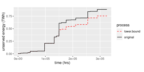
Figure 5: Example 2, 30% generation overcapacity: plot of cumulative unserved energy against time (black) together with lower bounding processes (red).

Again, for the case of 30% generation overcapacity, Figure 6 plots the percentage levels of energy in store during a two-year period, starting at time 265,000 hours and surrounding the one point in time at which the long store comes very close to emptying. The corresponding plot for 25% generation overcapacity is again very similar. In each case, the medium store cycles rapidly, thereby using its higher efficiency to greatly reduce the capacity and input rate requirements on the long store. It nevertheless generally reserves about half its capacity so that it is available to assist in any “emergency” in which the demand exceeds the output power of the long store alone. The exception to this occurs at those times when the long store is itself close to emptying, and when the medium store must therefore work harder to further relieve the pressure on the long store.

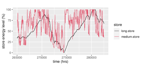
Figure 6: Example 2, 30% generation overcapacity: plot of store levels (%) against time.

Example 3.

Long (hydrogen) store with efficiency 0.4 plus short (Li-ion) store with efficiency 0.9. In the context of long-term GB storage needs, a necessarily relatively small short store (Li-ion battery) can probably only make a relatively modest contribution. Analogously to Example 2, we here explore the extent to which it is possible for it to assist in the provision of storage primarily provided by a long (hydrogen) store.

As in Example 2, we choose short (Li-ion) store dimensions which appear to work well with respect to overall cost minimisation, subject here to equal input and output power ratings—see the discussion above. (Again, we do not systematically optimise the short store dimensions, but considerable experimentation fails to produce any further decrease in the overall costs below). Given the short store dimensions, and subject to the given reliability standard, the long (hydrogen) store may again be optimally dimensioned—given the use of the value-function based scheduling algorithm, and to a very good approximation—as previously.

Table 4 shows storage dimensions and associated costs, again for both 30% and 25% generation overcapacity. These results are to be compared with those of Table 2. What is remarkable is that, for both levels of generation overcapacity, very large reductions in the capacity of the long (hydrogen) store are achieved through the introduction of a short (Li-ion) store of very small capacity. This is again primarily achieved through constant rapid cycling by the short store so as to exploit its much greater efficiency—see Figure 7 below. The total cost savings of $6.3 bn and $9.9 bn respectively, relative to the use of a single long store, are similarly noteworthy.

30% generation overcapacity                                                                            

		capacity	output power	input power	total cost
long	size	101.2    TWh	115.9 GW	77.5 GW
store	cost ($ bn)	81.0	49.7	66.5	197.2
short	size	0.085 TWh	15.0 GW	15.0 GW
store	cost ($ bn)	8.5	0.0	2.7	11.2
Total cost ($ bn)					208.4

25% generation overcapacity                                                                            

		capacity	output power	input power	total cost
long	size	136.8 TWh	112.0 GW	77.5 GW
store	cost ($ bn)	109.4	48.0	66.5	224.0
short	size	0.2 TWh	20.0 GW	20.0 GW
store	cost ($ bn)	20.0	0.0	3.6	23.6
Total cost ($ bn)					247.6

Table 4: Long (hydrogen) store plus short (Li-ion) store: dimensions and costs.

The parameters $\lambda_{i}$ of the scheduling algorithm (equation (10)) are given by $(\lambda_{l},\lambda_{s})=(0.000001,0.1)$ per hr and by $(\lambda_{l},\lambda_{s})=(0.0003,0.1)$ per hr respectively for 30% and 25% generation overcapacity. The average annual volumes of energy served externally by the long and short stores are 73.8 TWh and 9.8 TWh respectively in the case of 30% overcapacity, and 73.4 TWh and 15.8 TWh respectively in the case of 25% overcapacity—again with negligible extra energy being used for cross-charging.

For 30% generation overcapacity, Figure 7 plots the percentage levels of energy in store during the same two-year period considered in Example 2. It is seen that the short (Li-ion) store here devotes all its capacity to cycling rapidly, using its higher efficiency to greatly reduce the capacity and, to a lesser extent, the input power requirements for the long store. The capacity costs of the short store are such that it is not worth further increasing its capacity so as to reserve energy to enable the reduction of the output power requirement of the long store. Hence the pattern of usage of the short store is here different from that of the medium store in the previous example. The corresponding plot for 25% generation overcapacity is again very similar.

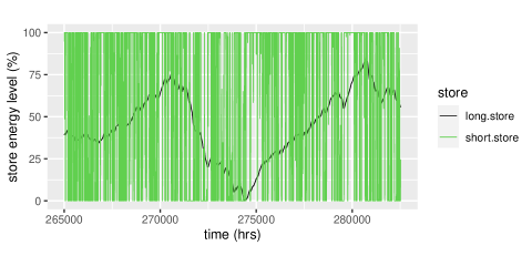
Figure 7: Example 3, 30% generation overcapacity: plot of store levels (%) against time.

Example 4.

Long (hydrogen) store with efficiency 0.4 plus medium (ACAES) store with efficiency 0.7 plus short (Li-ion) store with efficiency 0.9.

In this final example we take the set-up of Example 2, i.e. long (hydrogen) store plus medium (ACAES) store, and consider whether any further overall cost reduction can be obtained by the addition of a short (Li-ion) store. For both 30% and 25% generation overcapacity, some experimentation shows that the storage dimensions and associated costs given in Table 5 are at least approximately optimal and lead to modest cost reductions—relative to Example 2—of $0.34 bn and $1.12 bn respectively. In each case the short store is relatively very small indeed; however, variation of its dimensions does not seem to assist in further reducing overall costs. Thus, of our four examples, the present three-store mix appears to be the most economical; further, on the basis of the generation costs discussed above, the 30% level of generation overcapacity yields a net saving of $12 bn in comparison with the 25% level of overcapacity.

30% generation overcapacity                                                                            

		capacity	output power	input power	total cost
long	size	72.2   TWh	96.2 GW	53.3 GW
store	cost ($ bn)	57.8	41.3	45.7	144.8
medium	size	2.44  TWh	21.0 GW	21.1 GW
store	cost ($ bn)	22.0	4.2	4.2	30.4
short	size	0.005 TWh	2.0 GW	2.0 GW
store	cost ($ bn)	0.5	0.0	0.2	0.7
Total cost ($ bn)					175.8

25% generation overcapacity                                                                            

		capacity	output power	input power	total cost
long	size	78.9   TWh	81.0  GW	57.5  GW
store	cost ($ bn)	63.1	34.7	49.3	147.2
medium	size	4.25  TWh	40.0  GW	40.4  GW
store	cost ($ bn)	38.2	8.0	8.1	54.3
short	size	0.010 TWh	2.05 GW	2.05 GW
store	cost ($ bn)	1.0	0.0	0.4	1.4
Total cost ($ bn)					202.9

Table 5: Long (hydrogen) store plus medium (ACAES) store plus short (Li-ion) store : dimensions and costs.

The parameters $\lambda_{i}$ of the scheduling algorithm (equation (10)) are given by $(\lambda_{l},\lambda_{m},\lambda_{s})=(0.001,0.011,0.035)$ per hr and by $(\lambda_{l},\lambda_{m},\lambda_{s})=(0.0009,0.01,0.05)$ per hr respectively for 30% and 25% generation overcapacity. The annual volumes of energy served externally by the long, medium and short stores are 47.2 TWh, 36.4 TWh and 0.012 TWh respectively in the case of 30% generation overcapacity, and 38.5 TWh, 50.7 TWh and 0.027 TWh respectively in the case of 25% generation overcapacity, again with negligible extra energy being used for cross-charging.

For 30% generation overcapacity, Figure 8 plots the percentage levels of energy in store during the same two-year period considered in Examples 2 and 3. The behaviour of the long and medium store processes is, unsurprisingly, essentially as in Example 2. The behaviour of the short store is interesting. For most of the time it remains full, reserving its energy for those occasions on which it may be called on to act in an emergency. However, as the long and medium stores come close to being empty, the short store cycles as rapidly as possible—essentially in an attempt to prevent the former two stores actually emptying.

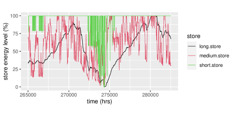
Figure 8: Example 4, 30% generation overcapacity: plot of store levels (%) against time.

5 Conclusions

Future electricity systems may well require extremely high volumes of energy storage with a mixture of storage technologies. This paper has studied the societal problems of scheduling and dimensioning such storage, with the scheduling objective of minimising total unserved energy over time, and the dimensioning objective of doing as economically as possible. We have identified properties of optimal scheduling policies and have argued that a value-function based approach is theoretically optimal. We have further shown that the optimal scheduling problem to be solved at each successive point in time reduces, to a good approximation, to a linear programme with a particularly simple solution.

We have been particularly concerned to develop non-anticipatory (without foresight) scheduling policies which are robust and suitable for real-time implementation, and have demonstrated their success in practical application. However, there are very occasional situations in which a forecast of, for example, a prolonged energy drought would make it sensible to modify scheduling policies so as to maximally conserve energy.

We have considered the practical application of the above theory to future GB energy storage needs, and shown, informally, how it may be used for the dimensioning of heterogeneous storage technologies. Notably, we have shown that the joint management of such technologies may greatly reduce overall costs (though the latter are as yet very uncertain).

We have not considered how to effect such storage dimensioning and management within a market environment in which storage is privately owned and operated by players each seeking to optimise their own returns. It seems likely that, under such circumstances, the effective use of storage would require management over extended periods of time by the electricity system operator and that contractual arrangements, including the possible introduction of storage capacity markets, would have to be such as to make this possible (see [27] for how this might be done).

Appendix: proofs

Proof of Proposition 1.

Given any feasible policy, we show how, for each successive time $t$, the policy may be modified at each time $t^{\prime}\geq t$ in such a way that the policy becomes greedy at the time $t$ and remains feasible at at each time $t^{\prime}\geq t$ (as well as at times prior to $t$), and further continues to serve at least as much energy in total to each successive time. Iterative application of this procedure over successive times $t$ then finally yields a policy which is feasible and greedy at all times and which continues to serve at least as much energy in total to each successive time. (Thus, at any time $t^{\prime}$, the final modification to the original policy is obtained by a succession of the above modifications associated with the successive times $t\leq t^{\prime}$.)

Suppose that, immediately prior and immediately subsequent to the modification associated with the time $t$ (which affects the storage rates and levels for those times $t^{\prime}\geq t$), the storage rates are defined, for each time $t^{\prime}$, respectively by $r(t^{\prime})=(r_{i}(t^{\prime}),\,i\in S)$ and $\hat{r}(t^{\prime})=(\hat{r}_{i}(t^{\prime}),\,i\in S)$, with the corresponding store levels being given respectively by $s(t^{\prime})=(s_{i}(t^{\prime}),\,i\in S)$ and $\hat{s}(t^{\prime})=(\hat{s}_{i}(t^{\prime}),\,i\in S)$, and with the total unserved energy to each successive time $t^{\prime}\geq t$ being given respectively by $\mathit{ue}(t)$ and $\hat{\mathit{ue}}(t^{\prime})$ as defined by (7). Then the modification associated with the time $t$ is defined as follows.

1. If $\mathit{re}(t)\geq 0$, increase (if necessary) the rates $(r_{i}(t),\,i\in S)$, at which energy is supplied to the stores at time $t$ to $(\hat{r}_{i}(t),\,i\in S)$, so that the policy becomes greedy at time $t$ while remaining feasible at that time. Note that the effect of this is to increase (weakly) the store levels at time $t$ so that $\hat{s}_{i}(t)\geq s_{i}(t)$, $i\in S$. For times $t^{\prime}>t$ and for each $i\in S$, set $\hat{r}_{i}(t^{\prime})=\min(r_{i}(t^{\prime}),E_{i}-s_{i}(t^{\prime}-1))$. Then the modified policy remains feasible and it is clear, by induction, that $\hat{s}_{i}(t^{\prime})\geq s_{i}(t^{\prime})$ for all $i\in S$ and for all $t^{\prime}\geq t$. Further, since $\mathit{re}(t)\geq 0$ there is no unserved energy at time $t$ and since, for $t^{\prime}>t$ such that $\mathit{re}(t^{\prime})<0$, we have $\hat{r}_{i}(t^{\prime})\leq r_{i}(t)$, $i\in S$ (implying, from (4), that the unserved energy $-u(t^{\prime})$ does not increase) it follows that the total unserved energy to each successive time $t^{\prime}\geq t$ does not increase.

2. If $\mathit{re}(t)<0$, reduce (if necessary) the rates $(r_{i}(t),\,i\in S)$, to $(\hat{r}_{i}(t),\,i\in S)$, so that the policy becomes greedy at time $t$ while remaining feasible at that time. For times $t^{\prime}>t$ and for each $i\in S$, set

   $$\hat{r}_{i}(t^{\prime})=\max(r_{i}(t^{\prime}),-s_{i}(t^{\prime}-1)).$$ (11)

   Then the modified policy remains feasible at each time $t^{\prime}>t$. We show by induction that, for all $t^{\prime}\geq t$,

   $$\mathit{ue}(t^{\prime})-\hat{\mathit{ue}}(t^{\prime})\geq\sum_{i\in S}(s_{i}(t^{\prime})-\hat{s}_{i}(t^{\prime})).$$ (12)

   For $t^{\prime}=t$, it is immediate from the definitions (1), (4) and (7) (and since $\mathit{re}(t)<0$), that (12) holds with equality. For $t^{\prime}>t$, assume the result (12) is true with $t^{\prime}$ replaced by $t^{\prime}-1$; we consider two cases:

   • if $\mathit{re}(t^{\prime})\geq 0$, then there is no unserved energy at time $t^{\prime}$ under any feasible policy, so that the left side of (12) remains unchanged between times $t^{\prime}-1$ and $t^{\prime}$, while, from (11), the right side of (12) decreases (weakly) between times $t^{\prime}-1$ and $t^{\prime}$; thus the inequality (12) continues to hold at time $t^{\prime}$;

   • if $\mathit{re}(t^{\prime})<0$, then, between times $t^{\prime}-1$ and $t^{\prime}$, both the right and left sides of (12) increase by $r_{i}(t^{\prime})-\hat{r}_{i}(t^{\prime})$, so that (12) again continues to hold at time $t^{\prime}$.

   It also follows by induction, using (11), that $\hat{s}_{i}(t^{\prime})\leq s_{i}(t^{\prime})$ for all $i\in S$ and $t^{\prime}\geq t$. Hence, from (12), it again follows that, under the modification associated with the time $t$, the total unserved energy to each successive time $t^{\prime}\geq t$ does not increase.

To show the second assertion of the proposition, observe that, under the above construction, the greedy policy finally associated with each time $t^{\prime}$ is defined entirely by the residual energy process $(\mathit{re}(t),\,t\leq t^{\prime})$ up to and including that time. ∎

Proof of Proposition 2.

For each time $t$, let $\hat{r}(t)=(\hat{r}_{i}(t),\,i\in S)$ be the vector of rates determined by the algorithm of the proposition, and let $\hat{u}(t)$ be the corresponding imbalance given by (4). It follows from Proposition 1 that, when the objective is the minimisation of total unserved energy over time, it is sufficient to consider greedy policies in which, at those times $t$ such that the residual energy $\mathit{re}(t)\geq 0$ the spilled energy $u(t)$ is minimised, and at those times $t$ such that the residual energy $\mathit{re}(t)<0$ the unserved energy $-u(t)$ is minimised. It is clear that, at each time $t$, the imbalance $\hat{u}(t)$ defined by the above algorithm achieves this minimisation in either case. Thus the problem of choosing, at each successive time $t$, a vector $r(t)$ of feasible rates so as to maximise the expression given by (8) reduces to that of choosing such a vector $r(t)$ so as to maximise $\sum_{i\in S}v^{t}_{i}(s)r_{i}(t)$ (where, again the state vector $s=s(t-1)$) subject to the additional constraint that the corresponding imbalance $u(t)$ defined by (4) is equal to $\hat{u}(t)$.

Assume, for the moment, that, at the given time $t$, the ordering of states by their charging or discharging priorities is in each case unique, i.e. that we do not have $\eta_{i}v^{t}_{i}(s)=\eta_{j}v^{t}_{j}(s)$ for any $i,j\in S$ or $v^{t}_{i}(s)=v^{t}_{j}(s)$ for any $i,j\in S$. Then the above vector of rates $\hat{r}(t)=(\hat{r}_{i}(t),\,i\in S)$ determined by the given algorithm is unique. Let $r(t)=\bar{r}(t)$ be the (or any) vector of rates which maximises $\sum_{i\in S}v^{t}_{i}(s)r_{i}(t)$ subject to the corresponding imbalance $\bar{u}(t)$ being equal to $\hat{u}(t)$ as required above. Let $S_{+}=\{i\in S\colon\bar{r}_{i}(t)>0\}$ and let $S_{-}=\{i\in S\colon\bar{r}_{i}(t)<0\}$. Then the rate vector $\bar{r}(t)$ satisfies the following four conditions, in each case since otherwise the above objective function $\sum_{i\in S}v^{t}_{i}(s)r_{i}(t)$ could clearly be increased, while maintaining the given imbalance constraint $\bar{u}(t)=\hat{u}(t)$:

1. subject to the constraint that the total amount charged to the stores is as given by $\sum_{i\in S_{+}}\bar{r}_{i}(t)$, both $S_{+}$ and the individual rates $\bar{r}_{i}(t)$, $i\in S_{+}$, are as determined by the store charging priorities defined by the proposition;

2. similarly, subject to the constraint that the total amount discharged by the stores is as given by $-\sum_{i\in S_{-}}\bar{r}_{i}(t)$, both $S_{-}$ and the individual rates $\bar{r}_{i}(t)$, $i\in S_{-}$, are as determined by the store discharging priorities defined by the proposition;

3. the condition (9) is satisfied for all $i\in S_{-}$, $j\in S_{+}$:

4. there are no pairs of stores $i,j\in S$ satisfying (9) such that it is possible to improve the solution $\bar{r}(t)$ by (further) cross-charging from $i$ to $j$.

It is now easy to see that the above conditions 1–4 are sufficient to ensure that $\bar{r}(t)$ is precisely as determined by algorithm, i.e. that $\bar{r}(t)=\hat{r}(t)$.

In the event that, at the given time $t$, the ordering of states by either their charging or discharging priorities is not unique (and so $\hat{r}(t)$ is not unique), it is easy to see that $\bar{r}(t)$, defined as above, may be adjusted if necessary—while continuing to maximise $\sum_{i\in S}v^{t}_{i}(s)r_{i}(t)$ subject to the given imbalance constraint—so that we again have $\bar{r}(t)=\hat{r}(t)$: one standard way to do this is to perturb $v^{t}_{i}(s)$, $i\in S$, infinitesimally so that the given $\hat{r}(t)$ becomes the unique solution of the scheduling algorithm, then let $\bar{r}(t)$ solve the given constrained maximisation problem as above, and then finally allow the perturbation to tend to zero to obtain the required result.

∎

References

- [1] D. Bertsekas “Dynamic Programming and Optimal Control: Volume I”, Athena scientific optimization and computation series v. 1 Athena Scientific, 2012 URL: https://books.google.co.uk/books?id=qVBEEAAAQBAJ
- [2] B. Cárdenas, L. Swinfen-Styles, J. Rouse and S.. Garvey “Short-, medium-, and long-duration energy storage in a 100% renewable electricity grid: a UK case study” In Energies 14.24, 2021 DOI: 10.3390/en14248524
- [3] J.. Cruise and S. Zachary “Optimal scheduling of energy storage resources”, 2018 URL: http://arxiv.org/abs/1808.05901
- [4] J.. Cruise and S. Zachary “The optimal control of storage for arbitrage and buffering, with energy applications” In Renewable Energy: Forecasting and Risk Management Springer, 2018, pp. 209–227 DOI: 10.1007/978-3-319-99052-1˙11
- [5] P. Denholm, E. Ela, B. Kirby and M.. Milligan “The role of energy storage with renewable electricity generation”, 2010 URL: https://www.nrel.gov/docs/fy10osti/47187.pdf
- [6] R. Durrett “Probability: Theory and Examples”, Cambridge Series in Statistical and Probabilistic Mathematics Cambridge University Press, 2019 URL: https://books.google.co.uk/books?id=vESPDwAAQBAJ
- [7] G. Edwards, S. Sheehy, C.. Dent and M… Troffaes “Assessing the contribution of nightly rechargeable grid-scale storage to generation capacity adequacy” In Sustainable Energy, Grids and Networks 12 Elsevier, 2017, pp. 69–81 DOI: 10.1016/J.SEGAN.2017.09.005
- [8] M. Evans, S.. Tindemans and D. Angeli “Robustly Maximal Utilisation of Energy-Constrained Distributed Resources” In 2018 Power Systems Computation Conference (PSCC), 2018, pp. 1–7 DOI: 10.23919/PSCC.2018.8443058
- [9] T. Gallo Cassarino, E. Sharp and M. Barrett “The impact of social and weather drivers on the historical electricity demand in Europe” In Applied Energy 229, 2018, pp. 176–185 DOI: 10.1016/J.APENERGY.2018.07.108
- [10] N.. Gast, D.. Tomozei and J-Y. Le Boudec “Optimal storage policies with wind forecast uncertainties” In Greenmetrics 2012, 2012 Imperial College, London, UK DOI: 10.1145/2425248.2425255
- [11] A… Khan, R.. Verzijlbergh, O.. Sakinci and L.. Vries “How do demand response and electrical energy storage affect (the need for) a capacity market?” In Applied Energy 214, 2018, pp. 39–62 DOI: 10.1016/j.apenergy.2018.01.057
- [12] Massachusetts Institute of Technology “The Future of Energy Storage”, 2022 URL: https://energy.mit.edu/wp-content/uploads/2022/05/The-Future-of-Energy-Storage.pdf
- [13] P. Nash and R. Weber “A simple optimizing model for reservoir control”, 1978
- [14] National Grid plc “Electricity Capacity Report”, 2018 URL: https://www.emrdeliverybody.com/Capacity%20Markets%20Document%20Library/Electricity%20Capacity%20Report%202018.pdf
- [15] National Grid plc “Electricity Capacity Reports”, 2022 URL: https://www.emrdeliverybody.com/CM/Capacity.aspx
- [16] D.. Newbery et al. “Benefits of an Integrated European Energy Market: Final Report for DG ENER”, 2013 URL: https://ec.europa.eu/energy/sites/ener/files/documents/20130902_energy_integration_benefits.pdf
- [17] D. Pudjianto, M. Aunedi, P. Djapic and G. Strbac “Whole-systems assessment of the value of energy storage in low-carbon electricity systems” In IEEE Transactions on Smart Grid 5, 2014, pp. 1098–1109 DOI: 10.1109/TSG.2013.2282039
- [18] T. Roulstone and P. Cosgrove “UK Multi-year Renewable Energy Systems with Storage - Cost Investigation”, 2022 DOI: 10.13140/RG.2.2.33695.43689
- [19] M.. Shaner, S.. Davis, N.. Lewis and K. Caldeira “Geophysical constraints on the reliability of solar and wind power in the United States” In Energy & Environmental Science 11.4, 2018, pp. 914–925 DOI: 10.1039/C7EE03029K
- [20] R. Sioshansi, S.. Madaeni and P. Denholm “A Dynamic Programming Approach to Estimate the Capacity Value of Energy Storage” In IEEE Transactions on Power Systems 29.1, 2014, pp. 395–403 DOI: 10.1109/TPWRS.2013.2279839
- [21] R. Sioshansi, P. Denholm, T. Jenkin and J. Weiss “Estimating the value of electricity storage in PJM: Arbitrage and some welfare effects” In Energy Economics 31.2, 2009, pp. 269–277 DOI: 10.1016/j.eneco.2008.10.005
- [22] Royal Society “Report of Working Group on Energy Storage”, To appear, 2022
- [23] I. Staffell and S. Pfenninger “Using bias-corrected reanalysis to simulate current and future wind power output” In Energy 114, 2016, pp. 1224–1239 DOI: 10.1016/j.energy.2016.08.068
- [24] G. Strbac et al. “Strategic Assessment of the Role and Value of Energy Storage Systems in the UK Low Carbon Energy Future”, 2012 URL: https://www.carbontrust.com/resources/energy-storage-systems-in-the-uk-low-carbon-energy-future-strategic-assessment
- [25] UK Committee on Climate Change “Net Zero – The UK’s contribution to stopping global warming”, 2019 URL: https://www.theccc.org.uk/publication/net-zero-the-uks-contribution-to-stopping-global-warming/
- [26] T. Weitzel and C.. Glock “Energy management for stationary electric energy storage systems: A systematic literature review” In European Journal of Operational Research 264.2, 2018, pp. 582–606 DOI: 10.1016/j.ejor.2017.06.052
- [27] S. Zachary, A. Wilson and C.. Dent “The integration of variable generation and storage into electricity capacity markets” In The Energy Journal 43, 2022 DOI: 10.5547/01956574.43.4.szac
- [28] S. Zachary et al. “Scheduling of energy storage” In Philosophical Transactions of the Royal Society A 397, 2021 DOI: 10.1098/rsta.2019.0435
- [29] Y. Zhou, P. Mancarella and J. Mutale “Modelling and assessment of the contribution of demand response and electrical energy storage to adequacy of supply” In Sustainable Energy, Grids and Networks 3, 2015, pp. 12–23 DOI: 10.1016/j.segan.2015.06.001