Warm Absorbers in the Radiation-driven Fountain Model of Low-mass Active Galactic Nuclei

Abstract

To investigate the origins of the warm absorbers in active galactic nuclei (AGNs), we study the ionization-state structure of the radiation-driven fountain model in a low-mass AGN (Wada et al., 2016) and calculate the predicted X-ray spectra, utilizing the spectral synthesis code Cloudy (Ferland et al., 2017). The spectra show many absorption and emission line features originated in the outflowing ionized gas. The O VIII 0.654 keV lines are produced mainly in the polar region much closer to the SMBH than the optical narrow line regions. The absorption measure distribution of the ionization parameter ($\xi$) at a low inclination spreads over 4 orders of magnitude in $\xi$, indicating multi-phase ionization structure of the outflow, as actually observed in many type-1 AGNs. We compare our simulated spectra with the high energy-resolution spectrum of the narrow line Seyfert 1 galaxy, NGC 4051. The model reproduces slowly outflowing (a few hundreds km s^-1) warm absorbers. However, the faster components with a few thousands km s^-1 observed in NGC 4051 are not reproduced. The simulation also underproduces the intensity and width of the O VIII 0.654 keV line. These results suggest that the ionized gas launched from sub-parsec or smaller regions inside the torus, which are not included in the current fountain model, must be important ingredients of the warm absorbers with a few thousands km s^-1. The model also consistently explains the Chandra/HETG spectrum of the Seyfert 2 galaxy, the Circinus galaxy.

1 Introduction

Outflows in various physical conditions are ubiquitously observed from an active galactic nuclei (AGN). They constitute essential elements of the AGN structure, such as jets, warm absorbers, narrow emission line regions (NLRs), and tori (e.g., Elitzur & Shlosman, 2006; Netzer, 2015; Wada et al., 2018b; Alonso-Herrero et al., 2021). By carrying a huge amount of mass, momentum, and energy from the nucleus, these AGN-driven outflows play key roles in determining the dynamics of accretion flow onto the supermassive black hole (SMBH), and even significantly affect its environment in the host galaxy or larger scale (e.g., Fabian, 2012; Harrison, 2017; Veilleux et al., 2020). Thus, revealing the physical properties and origins of the outflows is important to understand AGN feeding/feedback mechanisms.

Outflows of mildly ionized gas can be recognized in the ultraviolet (UV) to soft X-ray ($\lesssim$2 keV) spectrum of an AGN by blue-shifted absorption line and edge features (see e.g., Kaastra et al., 2000, 2002). They are phenomenologically referred to as “warm absorbers”, which are detected in the X-ray spectra of about half of nearby type-1 AGNs (e.g., Reynolds, 1997; Laha et al., 2014). With spectral fitting, one can derive the ionization parameter of the absorbers, $\xi=L_{\mathrm{ion}}/n_{\mathrm{H}}r^{2}$ (where $L_{\mathrm{ion}}$ is the AGN luminosity, $n_{\mathrm{H}}$ the hydrogen number density, and $r$ the distance from the ionizing source), the column density ($N_{\mathrm{H}}$), and the outflow velocity ($v_{\mathrm{out}}$). It is also possible to constrain $n_{\mathrm{H}}$ and/or $r$ using other diagnostics, such as population ratios among different energy levels of the same ions (e.g., Mao et al., 2017) and time variability (e.g., Krongold et al., 2007). The typical outflow velocities of the warm absorbers are a few hundred to a few thousand km s^-1. They show wide ranges of values in physical parameters such as $\xi$ and $N_{\mathrm{H}}$ (e.g., Kaastra et al., 2002; Kaspi et al., 2004; Behar et al., 2017), indicating multiphase nature of the AGN-driven outflows. Since their outflow velocities are low, the energy and momentum outflow rates carried by the warm absorbers are smaller and hence have less impacts on the environments compared with ultrafast outflows (UFOs), which have velocities of $\sim$0.1$c$ (e.g., Tombesi et al., 2010). However, due to their large mass outflow rates, the warm absorbers are important to understand the global processes of mass flow in AGN systems, e.g., what fraction of mass fed by the host galaxy is eventually accreted by the SMBH and is ejected back into the surroundings.

The physical origins of the warm absorbers still remain unclear, although several theoretical models have been proposed (e.g., Krolik & Kriss, 1995; Proga et al., 2000; Fukumura et al., 2010). Assuming that the outflow velocities of the warm absorbers correspond to the escape velocities from the gravitational potential of the SMBH, they are likely to be launched from outer accretion disks and/or torus regions. Mizumoto et al. (2019) have shown that the warm absorbers can be explained as thermally-driven winds from the broad line region and torus (see e.g., Krolik & Kriss 1995 for earlier works). However, they assume a very simplified geometry, whereas the real structures of the interstellar medium in the central region of AGNs are still unknown. Hence, it is quite important to investigate the origins of the warm absorbers on the basis of more realistic, physically motivated dynamical models.

Wada (2012) proposed a “radiation-driven fountain” model of an AGN based on three-dimensional radiation–hydrodynamic simulations. In this model, the outflows are driven mainly by the radiation pressure to dust and the thermal energy of the gas acquired via X-ray heating, and a geometrically thick torus-like shape is naturally formed (see Figure 1). Wada et al. (2016) applied this radiation-driven fountain model to the Circinus galaxy, which is one of the closest (4.2 Mpc: Freeman et al., 1977) type-2 AGN. The model is consistent with several observed features, such as the infrared spectral energy distribution (SED, Wada et al., 2016), the dynamics of atomic/molecular gas (Wada et al., 2018a; Izumi et al., 2018; Uzuo et al., 2021), distribution of ionized gas in the NLR (Wada et al., 2018b), and broadband X-ray spectra (Buchner et al., 2021). Mizumoto et al. (2019) also suggested that this kind of dust driven wind may play an important role to the warm absorber acceleration.

In this paper, we present the results of mock X-ray high energy-resolution spectroscopic observations based on the radiation-driven fountain in a low mass AGN produced by Wada et al. (2016). We adopt the same approach as in Wada et al. (2018b), which calculated the intensity maps of optical emission lines (H$\alpha$, H$\beta$, [O III], [N II], and [S II]) utilizing the Cloudy code (Ferland et al., 2017). The three dimensional density and velocity maps in a snapshot of the Wada et al. (2016) model are used as an input. Combining Cloudy runs along the radial direction, we make the map of the ionization state and calculate both the transmitted and scattered X-ray spectra at various inclination angles, which contain absorption and emission lines, respectively. Then, we compare these mock spectra with actual observations and investigate whether the observed spectral features of ionized absorbers (including both absorption and emission lines) can be explained by the radiation-driven fountain model.

We choose NGC 4051 (narrow line Seyfert 1) as the comparison target. It has similar AGN parameters to those assumed in the Wada et al. (2016) model; the black hole mass, bolometric luminosity, and Eddington ratio of NGC 4051 are ($\log M_{\mathrm{BH}}/M_{\odot}$, $\log L_{\mathrm{bol}}$, $\lambda_{\mathrm{Edd}}$) = ($5.6$, $43.2$, $0.33$). Extensive archival data of NGC 4051 observed with XMM-Newton are available. The high energy-resolution spectrum observed with the Reflection Grating Spectrometer (RGS) on XMM-Newton shows a number of complex emission/absorption features indicative of multiple warm absorbers. Thus, NGC 4051 is an ideal target for our study.

The structure of this paper is as follows. Section 2 describes the overview of the radiation-driven fountain model and the numerical methods of our Cloudy simulations. The results of the simulations are summarized in Sections 3. In Section 4, we compare our results with the observed X-ray spectrum of NGC 4051 and discuss the implications. Fe K$\alpha$ intensity distributions and comparison with the X-ray spectrum of the Circinus galaxy are shown in Appendix A.

2 Simulations

2.1 Input Model

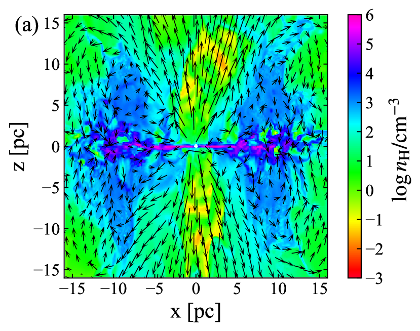
Figure 1: (a): A snapshot of hydrogen number-density distribution on a x-z plane in the radiation-driven fountain model (Wada et al., 2016). The arrows represent the relative velocity fields in logarithmic scales. (b): Same as (a), but for temperature distribution.

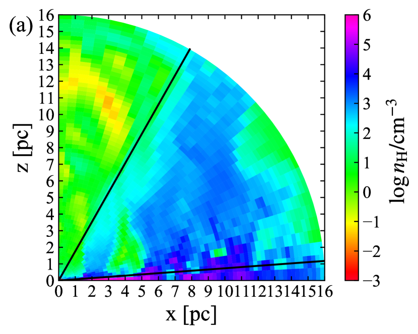
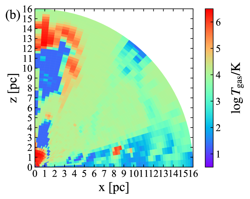
Figure 2: (a): Hydrogen number-density ($n_{\mathrm{H}}$) structure in a polar grid reformed from the original data in the radiation-driven fountain model. Black lines represents the lines of sight for $i=$ 30 and 86 degrees from z-axis. (b): Same as (a), but for the temperature ($T_{\mathrm{gas}}$) structure. (c): Structure of radial inflow or outflow velocities along the lines of sight ($v_{\mathrm{in}}$ and $v_{\mathrm{out}}$).

Here we summarize the assumptions of the radiation-driven fountain model by Wada et al. (2016), one of the dynamical models of AGN tori with supernova feedback based on three dimensional radiation-hydrodynamic simulations. The model only considers matter distribution in the torus region (0.125 pc $<r<$ 16 pc) but accounts for radiative feedback processes from the AGN such as the radiation pressure on the surrounding material and X-ray heating. The non-spherical radiation field caused by the AGN is considered. They set the black hole mass of $M_{\mathrm{BH}}$ to $2\times 10^{6}M_{\odot}$, the Eddington ratio $\lambda_{\mathrm{Edd}}$ to $0.2$, the bolometric luminosity $L_{\mathrm{bol}}$ to $5\times 10^{43}$ erg s^-1, and the X-ray luminosity (2–10 keV) $L_{\mathrm{X}}$ to $2.8\times 10^{42}$ erg s^-1. The solar metallicity and cooling functions for 20 K $\leq T_{\mathrm{gas}}\leq$ $10^{8}$ K (Meijerink & Spaans, 2005; Wada et al., 2009) are assumed, where $T_{\mathrm{gas}}$ is the temperature of gas. The hydrodynamics calculations cover (32 pc)³ region in the $256^{3}$ grid cells. Figure 1(a) and (b) show the distributions of gas density and temperature, respectively. The velocity field of gas is over-plotted in Figure 1(a).

2.2 Radiative Transfer

Following the quasi-three dimensional radiative transfer calculations in Wada et al. (2018b), we make use of Cloudy v17.02 (Ferland et al., 2017) to produce the ionization-state map and to simulate the spectra. We reform the cells from the $256^{3}$ Cartesian grid to the $64^{3}$ uniformly spaced polar grid. Figure 2 plots the geometry of the reformed model. We input the 3-dimensional maps of physical parameters (hydrogen density and temperature), obtained in a snapshot of the radiation-driven fountain model, into the Cloudy code. Figure 3 shows the input SED model at the innermost grids. It is equivalent to that obtained by the Cloudy’s AGN command and is represented as:

$$f\left(\nu\right)=\nu^{\alpha_{\mathrm{UV}}}\exp\left({-h\nu/kT_{\mathrm{BB}}}\right)\exp\left({-kT_{\mathrm{IR}}/h\nu}\right)\cos{i}$$

$$+a\nu^{\alpha_{\mathrm{X}}}\exp\left({-h\nu/E_{1}}\right)\exp\left({-E_{2}/h\nu}\right),$$ (1)

where $\alpha_{\mathrm{UV}}=-0.5$, $T_{\mathrm{BB}}=10^{5}$ K, $\alpha_{\mathrm{X}}=-0.7$, $a$ is a constant that yields the X-ray to UV ratio $\alpha_{\mathrm{OX}}=-1.4$, $kT_{\mathrm{IR}}=0.01$ Ryd, $E_{\mathrm{1}}=300$ keV, $E_{\mathrm{2}}=0.1$ Ryd, and $i$ is the angle from the z-axis (i.e., inclination). The UV radiation (first term), which comes from the geometrically thin, optically-thick disk, is assumed to be proportional to $\cos{i}$. Whereas, the X-ray component (second term) is assumed to be isotropic.

We run a sequence of Cloudy simulations along the radial direction from the central source to the outer boundary at $r=16$ pc, where the output spectrum (net transmitted spectrum, which is the sum of the attenuated incident radiation and the diffuse emission emitted by the photo-ionized plasma) from a cell is used as the input spectrum to the next (outer) cell by taking into account the velocity field of each cell. redHere, we assume that the density structure in each cell is uniform. For simplicity, we also assume that the net transmitted radiation is the primary ionizing source and the scattered radiation from the surrounding regions out of the line of sight is ignored. To confirm the validity of this assumption, we calculate the differences of the ionization parameters $\xi$ when the scattered components from the adjacent cells out of the line of sight are added to the input spectrum in each run. To estimate the scattered components, we utilize “the reflected spectra” calculated by Cloudy, which contains Compton-scattered incident radiation and the diffuse emission. We find that the increase in the $\xi$ parameter is $\sim$2% on average, except for a few grid cells in the equatorial plane ($>$100%). Thus, we restrict the analysis for the inclination angle to $i\leq 88^{\circ}$. After we calculate the ionization state and spectra in all cells, we integrate the reflected spectra over all cells by taking into account the optical depths in each cell along the line of sight. We refer to it as “scattered spectra” in the following.

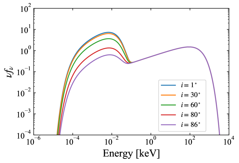
Figure 3: Incident SED models of the AGN at the innermost grids for inclination angle of $i=$ 1, 30, 60, 80, and 86 degrees (from top to bottom). The vertical axis has an arbitrary unit of $\nu f_{\nu}$, where $f_{\nu}$ is the energy flux at the frequency $\nu$.

3 Results

3.1 Ionization Structure

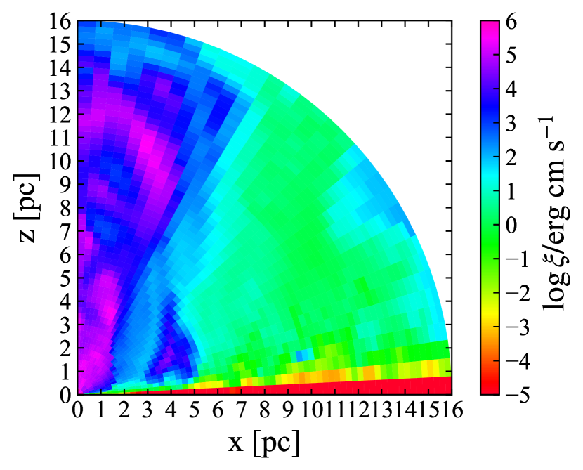
Figure 4: Structure of the ionization parameter ($\xi$) obtained by the Cloudy calculation.

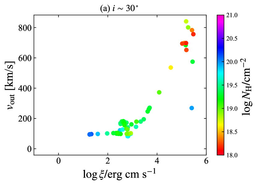
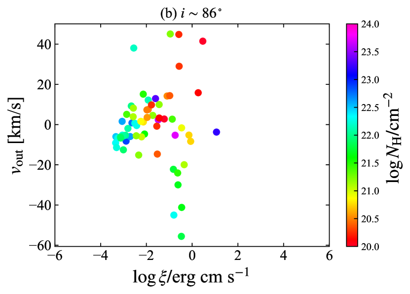
Figure 5: Relation between the ionization parameter ($\xi$) and the outflow velocity ($v_{\mathrm{out}}$) for the grid cells along a line of sight. Each data point is color-coded by the hydrogen column density in the cell. (a): for $i=30$ degrees. (b): for $i=86$ degrees.

Figure 4 plots the map of the ionization parameter, $\xi=L_{\mathrm{ion}}/n_{\mathrm{H}}r^{2}$. The ionization parameter is distributed over a wide range and shows a complex structure, which mainly reflects that of hydrogen density (Figure 2(a)). It is also seen that non-isotropic radiation from the central accretion disk makes the gas in the polar region more highly ionized ($\log\xi>3$) than that in higher inclination regions with the same hydrogen density and distance.

Figure 5 plots the relation between the ionization parameter ($\xi$) and the outflow velocity ($v_{\mathrm{out}}$) for the cells along a line of sight, where each data point is color-coded by the hydrogen column density of that cell. We show the results for two inclination angles, $i=$ 30 and 86 degrees, which are representative of type-1 and type-2 AGNs, respectively (see section 4.2 and Appendix A). As noticed, at the low inclination angle (Figure 5(a)), $\xi$ is well correlated with $v_{\mathrm{out}}$, except for the highest ionization states corresponding to the closest region to the SMBH. In the polar region, the gas is almost spherically expanding, and therefore from mass conservation, we expect that $v_{\mathrm{out}}\propto 1/(n_{\mathrm{H}}r^{2})$ and hence $\xi\propto v_{\mathrm{out}}$. By contrast, no clear correlation is found for the high inclination case (Figure 5(b)). In the region closer to the equatorial plane, the gas motion is dominated by random motion caused by the backflow, turbulence, and supernova feedback, rather than the coherent motion of outflow. This makes $v_{\mathrm{out}}$ smaller ($<$40–60 km s^-1) and more complex. See for example, Wada & Norman (2002); Kawakatu & Wada (2008), on the effect of supernova feedback on the turbulent structures of the circumnuclear disk. Note that the radiation-driven outflows from which the warm absobers are originated are not directly affected by the supernova feedback. It is notable that the column density is large ($\log N_{\mathrm{H}}>24$ in total) and radial velocity is relatively slow (a few tens of km s^-1) in this region.

3.2 X-ray Spectra

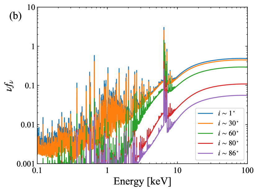
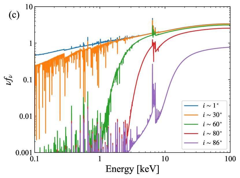
Figure 6: The simulated X-ray spectral models in units of $\nu f_{\nu}$ for inclinations of $i=$ 1, 30, 60, 80, and 86 degrees, from top to bottom. (a): The transmitted spectra (attenuated incident radiation). (b): The scattered spectra, which contains Compton scattered incident radiation and diffuse emission from all the cells. (c): The total (transmitted + scattered) spectra.

Figure 6(a), (b), (c) plot examples of the transmitted, scattered, and total spectra, respectively, for five inclination angles ($i=$ 1, 30, 60, 80, and 86 degrees). The spectra are characterized by many absorption line and edge features and emission lines. The transmitted spectra are absorbed by materials in the line of sight, and show many absorption lines by ionized gas in the 0.1–2 keV bandpass at low to medium inclination angles, whereas the absorption features are very weak at $i=1$ degree because of the low line-of-sight hydrogen column density. These results indicate that, even if the presence of warm absorbers is universal in AGNs, they can be directly observed only in a certain range of inclination angles. Ionized emission lines such as hydrogen and helium-like oxygen lines at $\sim$0.654 keV and 0.56 keV, respectively, are seen in the scattered spectra in all inclination angles. In addition to the emission lines from mildly to highly ionized gas (e.g., O VIII Ly$\alpha$ and O VII He$\alpha$ lines), iron K$\alpha$ fluorescence lines at $\sim$6.4 keV from cold matter is also produced.

3.3 O VIII Ly$\alpha$ Intensity Distribution

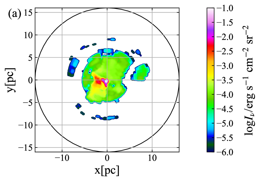
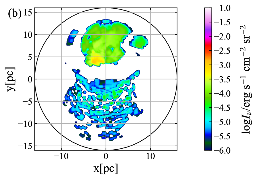
Figure 7: (a): Surface brightness distribution of O VIII Ly$\alpha$ at 0.654 keV for the inclination angle $i=0^{\circ}$. (b): Same as (a) but for $i=30^{\circ}$.

The Cloudy simulations enable us to investigate the spatial distribution of line intensity emitted by the irradiated gas. To make a surface brightness map that could be compared with a virtual high-spatial resolution observation, we integrate the line intensity along the lines of sight, taking into account absorption in each cell according to the optical depth. Figure 7(a) and (b) plot the surface brightness maps at 0.654 keV (corresponding to Ly$\alpha$ of O VIII) viewed from $i=0^{\circ}$ and 30^∘, respectively. As noticeable from the map at $i=30^{\circ}$, the lines produced in the upper side of the outflow are dominant in the observed spectrum because those in the bottom side are largely absorbed by the intervening gas. The gap at $y=$ 0–5 pc is due to the absorption by the optically thick, inner torus region. The O VIII distribution shows a conical shape similar to [O III] 5007 Å (Wada et al., 2018b), although the O VIII Ly$\alpha$ emitting region is located closer to the SMBH than the [O III] 5007 Å.

4 Comparison with Observations

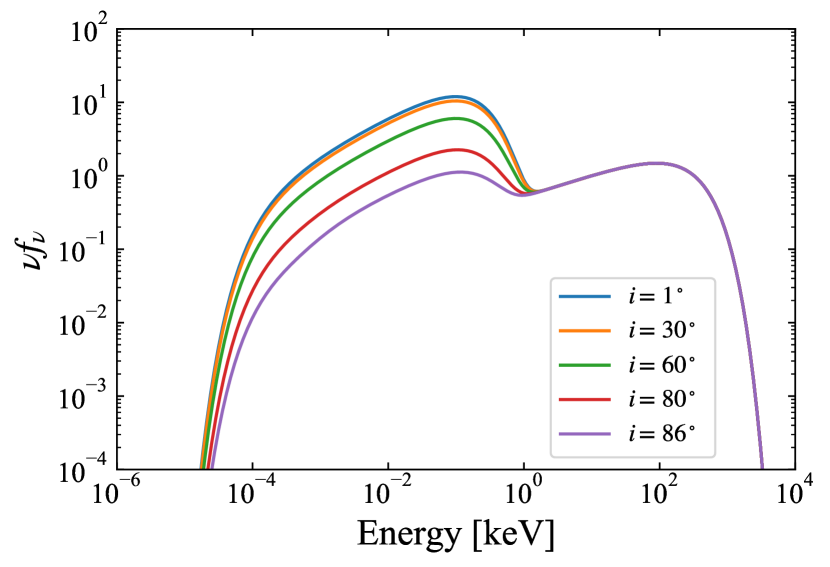
Figure 8: Incident SED models of NGC 4051 at the innermost grids for inclination angle of $i=$ 1, 30, 60, 80, and 86 degrees (from top to bottom). The vertical axis has an arbitrary unit of $\nu f_{\nu}$.

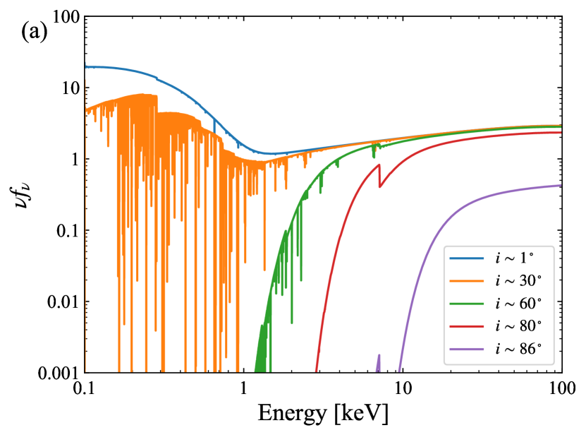
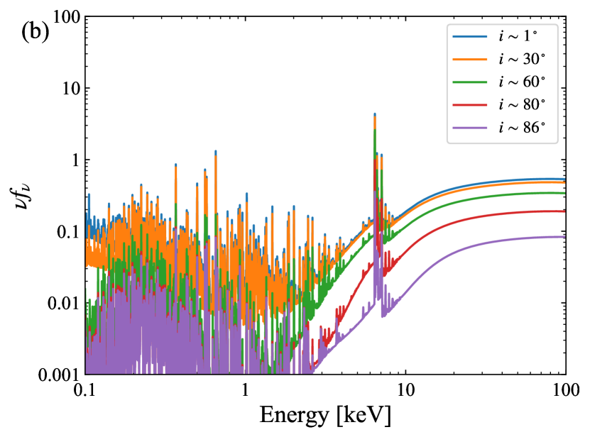
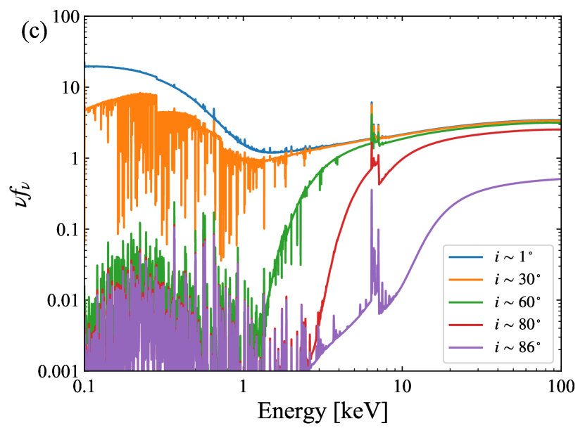
Figure 9: The simulated X-ray spectral models for NGC 4051 in units of $\nu f_{\nu}$ for inclinations of $i=$ 1, 30, 60, 80, and 86 degrees, from top to bottom. (a): The transmitted spectra (attenuated incident radiation). (b): The scattered spectra, which contains Compton scattered incident radiation and diffuse emission from all the cells. (c): The total (transmitted + scattered) spectra.

In this section, we compare the results of our mock observations of a radiation-driven fountain with actual observations, regarding the properties of the ionized absorbers and X-ray spectra. For the comparison object with a low inclination, where the warm absorbers are directly observed, we have selected NGC 4051. For a high inclination case, we show the comparison with the Circinus galaxy (Seyfert 2) in Appendix A.2. Wada et al. (2016) adopted the same AGN parameters as those of the Circinus galaxy, ($\log M_{\mathrm{BH}}/M_{\odot}$, $\log L_{\mathrm{bol}}$, $\lambda_{\mathrm{Edd}}$) = ($6.3$, $43.7$, $0.2$).

In order to make a precise comparison with NGC 4051, we performed the Cloudy simulations by changing the input SED to that more suitable for NGC 4051. This is mainly because NGC 4051 shows a strong soft excess component in the 0.4–1 keV band over the power-law component (e.g., Nucita et al., 2010; Mizumoto & Ebisawa, 2017; Ogawa et al., 2021). To find an appropriate SED model of NGC 4051, we performed a SED fitting with the equation 2.2 using the time-averaged data of XMM-Newton (Jansen et al., 2001) EPIC/pn and optical monitor (OM). We derived $T_{\mathrm{BB}}=2\times 10^{6}$ K, $\alpha_{\mathrm{X}}=-0.7$, and $\alpha_{\mathrm{OX}}=-1.3$. The other parameters are fixed at the values adopted in the previous simulations. Since $T_{\mathrm{BB}}$ is 20 times larger than that in Wada et al. (2018b), the prominent soft excess component appears in the 0.4–1 keV band. The ionizing luminosity $L_{\mathrm{ion}}$ (0.0136–13.6 keV) and the ionization parameters $\xi$ are increased by a factor of $\sim$5 (i.e., $\log\xi$ is increased by $\sim$0.7) compared with the original SED. We assumed that the contamination from the host galaxy has negligible effects on the OM data. Figures 8 shows input SED models at five inclination angles ($i=$ 1, 30, 60, 80, and 86 degrees). The output spectra of the transmitted, scattered, and total components are plotted in Figure 9.

Note that the SED assumed in the Cloudy simulation for NGC 4051 are not strictly the same as those assumed for the Circinus galaxy (Wada et al., 2016) (see Figures 3 and 8). However, as Wada (2015) showed, the structure of the radiation-driven fountain will not change significantly as long as the Eddington ratio is similar (in the range of 0.2–0.3). Therefore, we here try to compare the fountain model and the X-ray warm absorbers in NGC 4051.

4.1 Ionized Absorbers

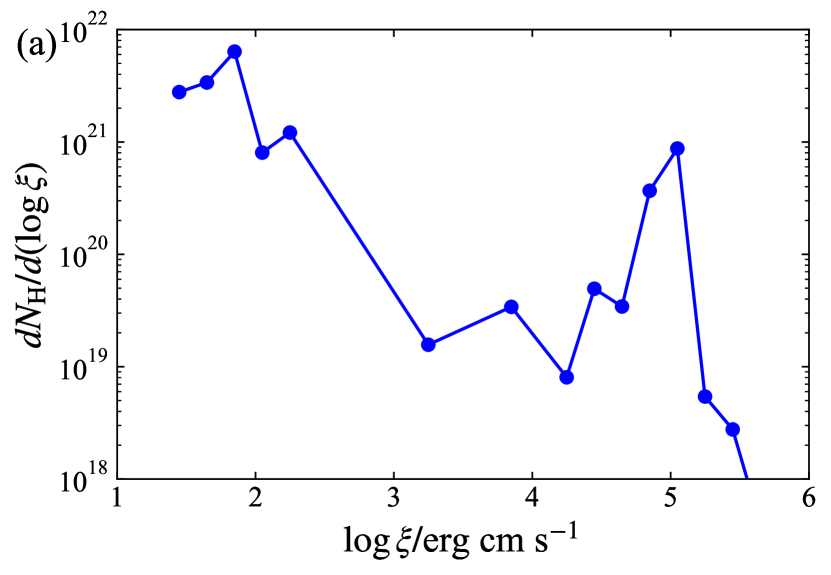
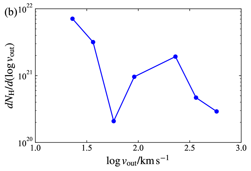
Figure 10: Model predicted absorption measure distributions (AMDs) for $i=$ 30 degrees, which corresponds to the best-fit inclination angle of NGC 4051. (a): that of $\log\xi$. (b): that of $\log v_{\mathrm{out}}$.

We investigate the absorption measure distribution (AMD) of $\xi$ and $v_{\mathrm{out}}$, which provides quantitative information on the ionization and velocity structures of an outflow. Several attempts have been made to derive the AMDs utilizing high-resolution X-ray spectra of type-1 AGNs. In most cases, the AMDs have been found to be multi-peaked, indicating the presence of multi-phase ionized absorbers along the line of sight (e.g., Holczer et al., 2007; Adhikari et al., 2019). We adopt the definition by Holczer et al. (2007) for the AMD as a function of the parameter $x$:

$$\mathrm{AMD}\left(x\right)\equiv\frac{dN_{\mathrm{H}}}{d\left(\log x\right)}.$$ (2)

Figure 10 displays the AMDs of ionization parameter $\xi$ and of outflow velocity $v_{\mathrm{out}}$ obtained at $i=30^{\circ}$ from our simulation data. As noticed, they spread over wide ranges of the parameters. In NGC 4051, ionization parameters and outflow velocities of multiple warm absorbers are consistent with our AMDs ($\log\xi=1.4-5$ and $\log v_{\mathrm{out}}=2.3-2.8$ have been actually observed: Krongold et al. 2007; Steenbrugge et al. 2009; Lobban et al. 2011; Pounds & Vaughan 2011; King et al. 2012; Silva et al. 2016; Mizumoto & Ebisawa 2017). These slow ionized absorbers whose $v_{\mathrm{out}}$ are a few hundreds km s^-1 may be interpreted as the origin of the warm-absorber outflow from the torus scale (Blustin et al., 2005).

Here we make detailed comparison with the results of Lobban et al. (2011), who reported that four distinct ionization zones with outflow velocities of $<$1000 km s^-1 were required to reproduce the Chandra/HETG data of NGC 4051 observed in 2008 November. Our AMD gives a reasonably good description of their zones 3a, 3b, and 4, whose warm absorber parameters are ($\log N_{\mathrm{H}}$, $\log\xi$, $\log v_{\mathrm{out}}$) = ($21.0$, $2.16$, $2.74$), ($20.7$, $1.96$, $2.91$), and ($21.4$, $2.97$, $2.85$), respectively. On the other hand, zones 1 and 2, which have ($\log N_{\mathrm{H}}$, $\log\xi$, $\log v_{\mathrm{out}}$) = ($20.5$, $-0.86$, $2.25$) and ($20.2$, $0.60$, $2.34$), respectively, are not reproduced in our model; their ionization parameters are much lower than those in our model. To reproduce these low ionization, low column-density material, numerical simulations with higher spatial resolution may be needed. Assuming $L_{\mathrm{ion}}=10^{43}$ erg s^-1, $\xi=L_{\mathrm{ion}}/n_{\mathrm{H}}r^{2}=1$, and $r=$10 pc, where $\log v_{\mathrm{out}}$ is $\sim$2 (Figure 2(c)), $n_{\mathrm{H}}\sim 10^{4}$ cm^-3 and therefore $N_{\mathrm{H}}=n_{\mathrm{H}}\Delta r\sim 10^{22}$ cm^-2 for $\Delta r$ = 0.25 pc, which is the resolution along the radial direction in this work. To reproduce the observed low column densities of zones 1 and 2, clumpy gas whose size is 1.5–2 orders of magnitude smaller than the current resolution must be considered.

In addition to these relatively slow components, faster ones with $v_{\mathrm{out}}>4000$ km s^-1 are also detected (Steenbrugge et al., 2009; Lobban et al., 2011; Pounds & Vaughan, 2011; Silva et al., 2016; Mizumoto & Ebisawa, 2017). The latter cannot be reproduced by our current model. This is because the model does not include any matter inside the innermost numerical grid (i.e., $r=0.125$ pc), where the escape velocities for a black hole mass of $2\times 10^{6}M_{\odot}$ are $>$370 km s^-1. Assuming that the outflow velocity corresponds to the escape velocity, these faster outflows should be launched at regions closer to the SMBH than the torus, such as the line-driven wind (e.g., Nomura & Ohsuga, 2017; Nomura et al., 2020, for UFOs). In fact, recent radiation-hydrodynamic simulations suggest that, if the dusty gas of a thin disk continues to the inner 0.01 pc under the non-spherical UV radiation field, the gas can be blown away with outflow velocities of $>$1000 km s^-1 (Kudoh, Y., et al., in preparation). This fast outflow may be able to explain the properties of the observed fast warm absorbers. Another possibility is the magnetically driven outflows (e.g., Fukumura et al., 2010, 2014), but simulations of magnetic winds depend on the (currently unknown) magnetic field configuration.

4.2 X-ray Spectrum

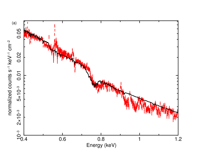
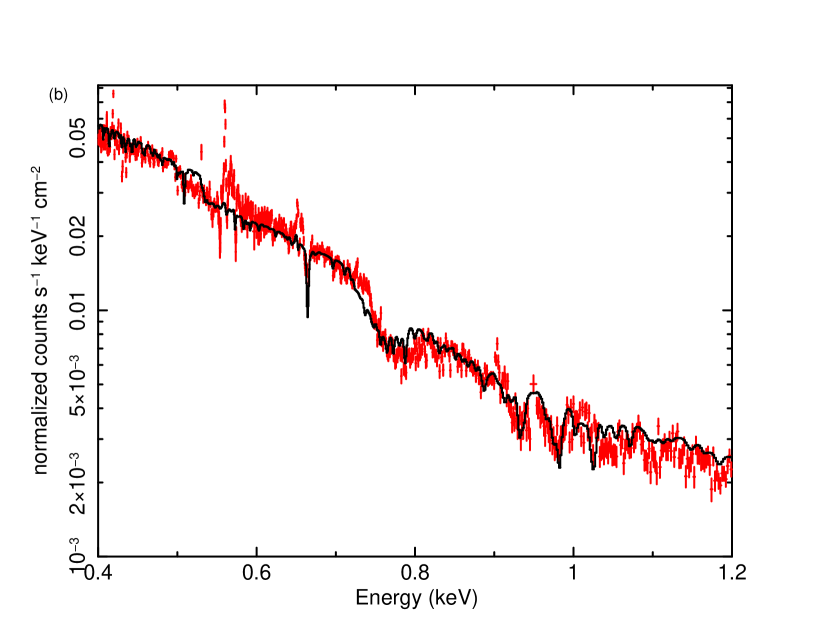
Figure 11: (a): The spectrum of NGC 4051 observed with XMM-Newton/RGS (red crosses). It is folded with the energy responses but is corrected for effective area. The solid curve represents the best-fit model based on our Cloudy simulations. (b): Same as (a), but fit with the model including a fast warm-absorber component.

We compare our simulated spectra with the high energy-resolution spectrum of NGC 4051 observed with XMM-Newton/RGS(den Herder et al., 2001). Our purpose is to check to what extent our simulations may produce the observed spectrum, in order to obtain insights on the AGN structure. Efforts to find spectral models that are fully consistent with the observed spectrum are beyond the scope of this paper.

We analyzed the archival data observed in 2009 May–June (observation ID: 0606320101, 0606320201, 0606320301, 0606320401, 0606321301, 0606321401, 0606321501, 0606321601, 0606321701, 0606321801, 0606321901, 0606322001, 0606322101, 0606322201, 0606322301) using the Science Analysis Software (SAS) version 17.0.0 and calibration files (CCF) released on 2018 June 22. These observation epochs are different from that of the Chandra/HETG observation discussed in the previous subsection (Lobban et al., 2011). The RGS data were reprocessed with rgsproc. We stacked all the data to create the highest signal-to-noise time-averaged spectrum.

We fit the spectrum in the 0.4–1.6 keV range with a model based on our simulations using the Cash statistic (Cash, 1979). In the Xspec terminology, the model is represented as “phabs $\times$ (mtable{fountain_T.fits} $\times$ zcutoffpl1 + zcutoffpl2 $+$ atable{fountain_S.fits})”. The phabs term represents the Galactic absorption fixed at $N_{\mathrm{H}}=1.20\times 10^{20}$ cm^-2 (the total Galactic H I and H₂ value given by Willingale et al. 2013). We use the zcutoffpl1 and zcutoffpl2 to represent the first and second terms in Equation 2.2, respectively. The table model atable{fountain_S.fits} represents scattered spectra of our simulation, whereas mtable{fountain_T.fits} takes into account the absorption to the transmitted component. The free parameters are the cutoff energy and normalization of zcutoffpl1, the normalization of zcutoffpl2, and the inclination and azimuthal angles in the two table models. The normalization of atable{fountain_S.fits} is linked to that of zcutoffpl2, the photon index of zcutoffpl1 is fixed at 1.5, and the photon index and cutoff energy of zcutoffpl2 are fixed at 1.7 and 300 keV, respectively.

Figure 11(a) plots the observed spectrum of NGC 4051 and the best-fit model folded with the energy responses (corrected for the effective area). We obtain the best-fit inclination angle of $\approx$30^∘ ($C/$dof $=9621/2304$). It is seen that our model reproduces many weak absorption features, particularly at energies below 0.6 keV. As mentioned above, however, it cannot reproduce the strong absorption features at $\geq$0.9 keV, which are produced by fast warm absorbers with $v_{\mathrm{out}}\sim$ 4000–6000 km s^-1 (Pounds & Vaughan, 2011; Silva et al., 2016; Mizumoto & Ebisawa, 2017). If a fast component with $\log\xi\sim 2.6$, $\log N_{\mathrm{H}}\sim 22.2$, $v_{\mathrm{out}}\sim 4700$ km s^-1 is added to our model, these absorption features can be reproduced (Figure 11(b)) and the fit is much improved ($C/$dof $=7944/2301$).

It is also noteworthy that the simulated spectra have weaker emission lines than the observed data; the equivalent width of O VIII Ly$\alpha$ is by a factor of $\sim$8 smaller than that of observed result (Mizumoto & Ebisawa, 2017). These emission lines may also come from regions inside the space where the hydrodynamic simulations were performed (i.e., $<$0.125 pc). In fact, the line width of O VIII Ly$\alpha$, $\sigma=0.1$ Å (Mizumoto & Ebisawa, 2017) (or 1600 km s ^-1), is too broad to be produced by our model. Fast warm absorbers launched at $r<$0.125 pc (see section 4.1) might produce these emission lines.

Our model also shows some discrepancies with the observed spectrum in the Fe M-shell unresolved transition array (UTA) feature around 0.7 keV. This is mainly because the the column density and outflow velocity of the best-fit model do not correctly represent those It is also noticeable that the model overestimates the flux around 0.5–0.53 keV. We infer that this is because the model does not well reproduce the K-edge feature from H-like carbon ions at 0.49 keV(Kramida et al., 2020). At the best-fit inclination angle, which is mainly determined by the UTA feature, carbon atoms are almost fully ionized and hence the edge structure is very weak. Here, one should also note that the three dimensional substructures of the absorbers could be highly time variable. In fact, as Schartmann et al. (2014) showed (see their Figure 6), the observed SEDs, especially in the short wavelengths, varies more than two orders of magnitude due to the absorption for a given inclination angle over 0.1–1 Myr.

5 Conclusions

1. We have investigated the ionization state and X-ray spectra of the radiation-driven fountain model around a low-mass AGN (Wada et al., 2016), utilizing the Cloudy code.

2. The model makes multi-phase ionization structure around the SMBH, as is actually observed in ionized outflows of AGNs. The simulated spectra show many absorption features and emission lines of ionized materials, which highly depends on inclination angle.

3. We compare our mock observations with the actual spectrum of NGC 4051. Although the radiation-driven fountain model accounts for warm absorbers with low ionization parameters ($\log\xi\lesssim 2$) and low outflow velocities of $>$a few hundred km s^-1, it cannot reproduce faster ones with a few thousands km s^-1. Also, our simulated spectra show a weaker and narrower O VIII Ly$\alpha$ emission line than the observed one by factors of $\sim$8 and $\sim$2, respectively.

4. These results suggest that additional components originated from the region closer to the SMBH than the torus via e.g., line-driven winds produced in the accretion disk, must be an important ingredient of the warm absorbers in AGNs.

Appendix A Cold Reflectors in the Radiation-Driven Foutain Model

For reference, we also investigate the nature of cold reflectors in the radiation-driven fountain model, with a particular focus on the fluorescence Fe K$\alpha$ line.

A.1 Fe K$\alpha$ Intensity Distribution

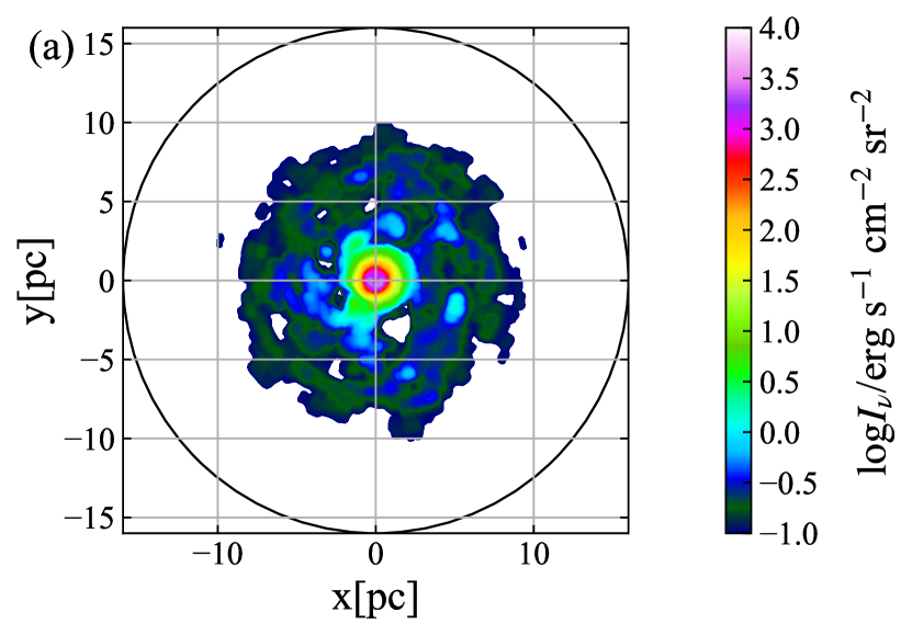
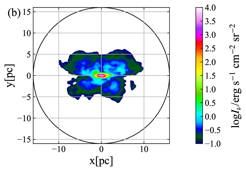
Figure 12: (a): Surface brightness distribution of Fe K$\alpha$ at 6.4 keV for $i=0^{\circ}$. (b): Same as (a) but for $i=80^{\circ}$.

Figure 12(a) and (b) plot the surface brightness maps of lowly ionized Fe K$\alpha$ lines at 6.4 keV. When viewed from nearly edge-on, the Fe K$\alpha$ lines mainly come from the far side of the inner torus. This is consistent with the results of a clumpy torus model (XCLUMPY; Tanimoto et al., 2019) studied by Uematsu et al. (2021), who investigated the locations of Fe K$\alpha$ emitting regions with Monte-Carlo ray-tracing simulations.

A.2 X-ray Spectrum: Comparison with Circinus Galaxy

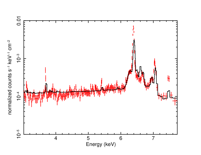
Figure 13: The spectrum of the Circinus galaxy observed with Chandra/HETG (red crosses). It is folded with the energy responses but is corrected for effective area. The solid curve represents the best-fit model based on our Cloudy simulations.

We also compare our simulated spectra with the observed data of the Circinus galaxy, to which the AGN parameters in Wada et al. (2016) are tuned (Section 2.1). We utilize the High-Energy Transmission Grating (HETG: Canizares et al., 2005) on Chandra (Weisskopf et al., 2002) spectrum as used in Uematsu et al. (2021). They analyzed the data from all 13 observations (observation ID: 374, 62877, 4770, 4771, 10226, 10223, 10832, 10833, 10224, 10844, 10225, 10842, 10843), and created the time-averaged spectrum for a total exposure of 0.62 Ms. We adopt the model in the Xspec terminology “phabs $\times$ (zcutoffpl $+$ atable{fountain_S.fits} $+$ zgauss)”. The phabs and atable{fountain_S.fits} terms are the same as those of the model for NGC 4051. The zcutoffpl term also corresponds to the zcutoffpl2 term of the model for NGC 4051. The Galactic absorption is fixed at $N_{\mathrm{H}}=7.02\times 10^{21}$ cm^-2. We add zgauss as the Compton shoulder component of Fe K$\alpha$ line at 6.4 keV, which cannot be reproduced in the Cloudy code, where multiple scattering processes are ignored.

The observed spectrum and the best-fit model folded with the energy responses of the Circinus galaxy are plotted in Figure 13. We obtain the best-fit inclination angle of $\sim$87^∘, which is consistent with the previous studies, in which the infrared SED, molecular lines in radio, and X-ray continuum spectra are compared with observed ones (Wada et al., 2016; Izumi et al., 2018; Uzuo et al., 2021; Buchner et al., 2021). Our model gives a reasonably good description of observed spectrum except the intensities of the emission lines. This indicates that additional contributions are needed, as in the case of NGC 4051. One candidate would be the disk located inside the torus region, and/or outflows launched from it. This may be in line with the argument by Buchner et al. (2021) that additional matter inside $r\sim 0.1$ pc is necessary to account for the shape of the broadband X-ray spectrum of the Circinus galaxy.

References

- Adhikari et al. (2019) Adhikari, T. P., Różańska, A., Hryniewicz, K., Czerny, B., & Behar, E. 2019, ApJ, 881, 78, doi: 10.3847/1538-4357/ab2dfc
- Alonso-Herrero et al. (2021) Alonso-Herrero, A., García-Burillo, S., Hoenig, S. F., et al. 2021, arXiv e-prints, arXiv:2107.00244. https://arxiv.org/abs/2107.00244
- Arnaud (1996) Arnaud, K. A. 1996, in Astronomical Society of the Pacific Conference Series, Vol. 101, Astronomical Data Analysis Software and Systems V, ed. G. H. Jacoby & J. Barnes, 17
- Barvainis (1987) Barvainis, R. 1987, ApJ, 320, 537, doi: 10.1086/165571
- Behar et al. (2017) Behar, E., Peretz, U., Kriss, G. A., et al. 2017, A&A, 601, A17, doi: 10.1051/0004-6361/201629943
- Blustin et al. (2005) Blustin, A. J., Page, M. J., Fuerst, S. V., Branduardi-Raymont, G., & Ashton, C. E. 2005, A&A, 431, 111, doi: 10.1051/0004-6361:20041775
- Buchner et al. (2021) Buchner, J., Brightman, M., Baloković, M., et al. 2021, A&A, 651, A58, doi: 10.1051/0004-6361/201834963
- Canizares et al. (2005) Canizares, C. R., Davis, J. E., Dewey, D., et al. 2005, PASP, 117, 1144, doi: 10.1086/432898
- Cash (1979) Cash, W. 1979, ApJ, 228, 939, doi: 10.1086/156922
- den Herder et al. (2001) den Herder, J. W., Brinkman, A. C., Kahn, S. M., et al. 2001, A&A, 365, L7, doi: 10.1051/0004-6361:20000058
- Elitzur & Shlosman (2006) Elitzur, M., & Shlosman, I. 2006, ApJ, 648, L101, doi: 10.1086/508158
- Fabian (2012) Fabian, A. C. 2012, ARA&A, 50, 455, doi: 10.1146/annurev-astro-081811-125521
- Ferland et al. (2017) Ferland, G. J., Chatzikos, M., Guzmán, F., et al. 2017, Rev. Mexicana Astron. Astrofis., 53, 385. https://arxiv.org/abs/1705.10877
- Freeman et al. (1977) Freeman, K. C., Karlsson, B., Lynga, G., et al. 1977, A&A, 55, 445
- Fukumura et al. (2010) Fukumura, K., Kazanas, D., Contopoulos, I., & Behar, E. 2010, ApJ, 715, 636, doi: 10.1088/0004-637X/715/1/636
- Fukumura et al. (2014) Fukumura, K., Tombesi, F., Kazanas, D., et al. 2014, ApJ, 780, 120, doi: 10.1088/0004-637X/780/2/120
- Gabriel et al. (2004) Gabriel, C., Denby, M., Fyfe, D. J., et al. 2004, in Astronomical Society of the Pacific Conference Series, Vol. 314, Astronomical Data Analysis Software and Systems (ADASS) XIII, ed. F. Ochsenbein, M. G. Allen, & D. Egret, 759
- Harrison (2017) Harrison, C. M. 2017, Nature Astronomy, 1, 0165, doi: 10.1038/s41550-017-0165
- Holczer et al. (2007) Holczer, T., Behar, E., & Kaspi, S. 2007, ApJ, 663, 799, doi: 10.1086/518416
- Izumi et al. (2018) Izumi, T., Wada, K., Fukushige, R., Hamamura, S., & Kohno, K. 2018, ApJ, 867, 48, doi: 10.3847/1538-4357/aae20b
- Jansen et al. (2001) Jansen, F., Lumb, D., Altieri, B., et al. 2001, A&A, 365, L1, doi: 10.1051/0004-6361:20000036
- Kaastra et al. (2000) Kaastra, J. S., Mewe, R., Liedahl, D. A., Komossa, S., & Brinkman, A. C. 2000, A&A, 354, L83. https://arxiv.org/abs/astro-ph/0002345
- Kaastra et al. (2002) Kaastra, J. S., Steenbrugge, K. C., Raassen, A. J. J., et al. 2002, A&A, 386, 427, doi: 10.1051/0004-6361:20020235
- Kaspi et al. (2004) Kaspi, S., Netzer, H., Chelouche, D., et al. 2004, ApJ, 611, 68, doi: 10.1086/422161
- Kawaguchi & Mori (2010) Kawaguchi, T., & Mori, M. 2010, ApJ, 724, L183, doi: 10.1088/2041-8205/724/2/L183
- Kawakatu & Wada (2008) Kawakatu, N., & Wada, K. 2008, ApJ, 681, 73, doi: 10.1086/588574
- King et al. (2012) King, A. L., Miller, J. M., & Raymond, J. 2012, ApJ, 746, 2, doi: 10.1088/0004-637X/746/1/2
- Koss et al. (2017) Koss, M., Trakhtenbrot, B., Ricci, C., et al. 2017, ApJ, 850, 74, doi: 10.3847/1538-4357/aa8ec9
- Kramida et al. (2020) Kramida, A., Yu. Ralchenko, Reader, J., & and NIST ASD Team. 2020, NIST Atomic Spectra Database (ver. 5.8), [Online]. Available: https://physics.nist.gov/asd [2021, October 5]. National Institute of Standards and Technology, Gaithersburg, MD.
- Krolik & Kriss (1995) Krolik, J. H., & Kriss, G. A. 1995, ApJ, 447, 512, doi: 10.1086/175896
- Krongold et al. (2007) Krongold, Y., Nicastro, F., Elvis, M., et al. 2007, ApJ, 659, 1022, doi: 10.1086/512476
- Laha et al. (2014) Laha, S., Guainazzi, M., Dewangan, G. C., Chakravorty, S., & Kembhavi, A. K. 2014, MNRAS, 441, 2613, doi: 10.1093/mnras/stu669
- Lobban et al. (2011) Lobban, A. P., Reeves, J. N., Miller, L., et al. 2011, MNRAS, 414, 1965, doi: 10.1111/j.1365-2966.2011.18513.x
- Mao et al. (2017) Mao, J., Kaastra, J. S., Mehdipour, M., et al. 2017, A&A, 607, A100, doi: 10.1051/0004-6361/201731378
- Meijerink & Spaans (2005) Meijerink, R., & Spaans, M. 2005, A&A, 436, 397, doi: 10.1051/0004-6361:20042398
- Mizumoto et al. (2019) Mizumoto, M., Done, C., Tomaru, R., & Edwards, I. 2019, MNRAS, 489, 1152, doi: 10.1093/mnras/stz2225
- Mizumoto & Ebisawa (2017) Mizumoto, M., & Ebisawa, K. 2017, MNRAS, 466, 3259, doi: 10.1093/mnras/stw3364
- Nasa High Energy Astrophysics Science Archive Research Center (2014) (Heasarc) Nasa High Energy Astrophysics Science Archive Research Center (Heasarc). 2014, HEAsoft: Unified Release of FTOOLS and XANADU, Astrophysics Source Code Library. http://ascl.net/1408.004
- Netzer (2015) Netzer, H. 2015, ARA&A, 53, 365, doi: 10.1146/annurev-astro-082214-122302
- Nomura & Ohsuga (2017) Nomura, M., & Ohsuga, K. 2017, MNRAS, 465, 2873, doi: 10.1093/mnras/stw2877
- Nomura et al. (2020) Nomura, M., Ohsuga, K., & Done, C. 2020, MNRAS, 494, 3616, doi: 10.1093/mnras/staa948
- Nucita et al. (2010) Nucita, A. A., Guainazzi, M., Longinotti, A. L., et al. 2010, A&A, 515, A47, doi: 10.1051/0004-6361/200913673
- Ogawa et al. (2021) Ogawa, S., Ueda, Y., Tanimoto, A., & Yamada, S. 2021, ApJ, 906, 84, doi: 10.3847/1538-4357/abccce
- Pounds & Vaughan (2011) Pounds, K. A., & Vaughan, S. 2011, MNRAS, 413, 1251, doi: 10.1111/j.1365-2966.2011.18211.x
- Proga et al. (2000) Proga, D., Stone, J. M., & Kallman, T. R. 2000, ApJ, 543, 686, doi: 10.1086/317154
- Reynolds (1997) Reynolds, C. S. 1997, MNRAS, 286, 513, doi: 10.1093/mnras/286.3.513
- Schartmann et al. (2014) Schartmann, M., Wada, K., Prieto, M. A., Burkert, A., & Tristram, K. R. W. 2014, MNRAS, 445, 3878, doi: 10.1093/mnras/stu2020
- Silva et al. (2016) Silva, C. V., Uttley, P., & Costantini, E. 2016, A&A, 596, A79, doi: 10.1051/0004-6361/201628555
- Steenbrugge et al. (2009) Steenbrugge, K. C., Fenovčík, M., Kaastra, J. S., Costantini, E., & Verbunt, F. 2009, A&A, 496, 107, doi: 10.1051/0004-6361/200810416
- Tanimoto et al. (2019) Tanimoto, A., Ueda, Y., Odaka, H., et al. 2019, ApJ, 877, 95, doi: 10.3847/1538-4357/ab1b20
- Tombesi et al. (2010) Tombesi, F., Cappi, M., Reeves, J. N., et al. 2010, A&A, 521, A57, doi: 10.1051/0004-6361/200913440
- Uematsu et al. (2021) Uematsu, R., Ueda, Y., Tanimoto, A., et al. 2021, ApJ, 913, 17, doi: 10.3847/1538-4357/abf0a2
- Uzuo et al. (2021) Uzuo, T., Wada, K., Izumi, T., et al. 2021, ApJ, 915, 89, doi: 10.3847/1538-4357/ac013d
- Veilleux et al. (2020) Veilleux, S., Maiolino, R., Bolatto, A. D., & Aalto, S. 2020, A&A Rev., 28, 2, doi: 10.1007/s00159-019-0121-9
- Wada (2012) Wada, K. 2012, ApJ, 758, 66, doi: 10.1088/0004-637X/758/1/66
- Wada (2015) —. 2015, ApJ, 812, 82, doi: 10.1088/0004-637X/812/1/82
- Wada et al. (2018a) Wada, K., Fukushige, R., Izumi, T., & Tomisaka, K. 2018a, ApJ, 852, 88, doi: 10.3847/1538-4357/aa9e53
- Wada & Norman (2002) Wada, K., & Norman, C. A. 2002, ApJ, 566, L21, doi: 10.1086/339438
- Wada et al. (2009) Wada, K., Papadopoulos, P. P., & Spaans, M. 2009, ApJ, 702, 63, doi: 10.1088/0004-637X/702/1/63
- Wada et al. (2016) Wada, K., Schartmann, M., & Meijerink, R. 2016, ApJ, 828, L19, doi: 10.3847/2041-8205/828/2/L19
- Wada et al. (2018b) Wada, K., Yonekura, K., & Nagao, T. 2018b, ApJ, 867, 49, doi: 10.3847/1538-4357/aae204
- Weisskopf et al. (2002) Weisskopf, M. C., Brinkman, B., Canizares, C., et al. 2002, PASP, 114, 1, doi: 10.1086/338108
- Willingale et al. (2013) Willingale, R., Starling, R. L. C., Beardmore, A. P., Tanvir, N. R., & O’Brien, P. T. 2013, MNRAS, 431, 394, doi: 10.1093/mnras/stt175