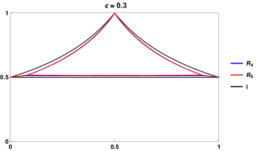
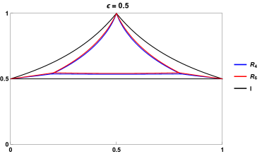
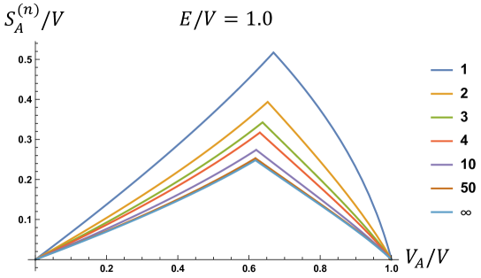
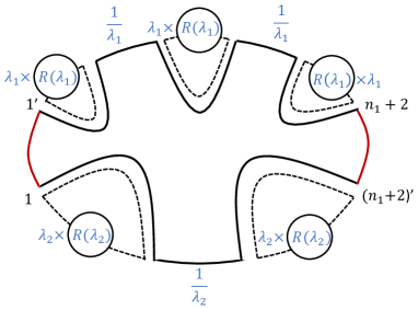
**footnotetext: These authors contributed equally to the work.

Mixed-state entanglement and information recovery in thermalized states and evaporating black holes

Shreya Vardhan    Jonah Kudler-Flam    Hassan Shapourian    and Hong Liu
Abstract

We study the universal behavior of quantum information-theoretic quantities in thermalized isolated quantum many-body systems and evaporating black holes. In particular, we study a genuine mixed-state entanglement measure called the logarithmic negativity, other correlation measures including the Renyi negativities and the mutual information, and a signature of multipartite entanglement called the reflected entropy. We also probe the feasibility of recovering quantum information from subsystems of a thermalized quantum many-body system or from the radiation of an evaporating black hole, using quantities such as relative entropy and Petz map fidelity. A recently developed technique called the equilibrium approximation allows us to probe these quantities at finite temperature. We find striking qualitative differences from the infinite temperature case, which has been the topic of previous studies using Haar-random states. In particular, we find regimes where the logarithmic negativity is extensive but the mutual information is sub-extensive, indicating a large amount of undistillable, bound entanglement in thermalized states. For evaporating black holes at finite temperature, both the logarithmic negativity and the Petz map fidelity reveal an important new time scale tbsubscript𝑡𝑏t_{b}, which is earlier than the Page time tpsubscript𝑡𝑝t_{p} by a finite fraction of the total evaporation time. We find that tbsubscript𝑡𝑏t_{b}, as opposed to tpsubscript𝑡𝑝t_{p}, is the time scale at which quantum entanglement between different parts of the radiation becomes extensive, and the fidelity of information recovery for a large diary thrown into the black hole starts to grow.

1 Introduction

A chaotic quantum many-body system initially in a far-from-equilibrium pure state should eventually approach a macroscopic equilibrium. In equilibrium, despite the fact that the system is in a pure state, we can use an equilibrium density operator ρ(eq)superscript𝜌(eq)\rho^{\text{(eq)}} to characterize its macroscopic properties using quantities such as temperature, thermal entropy, and free energy. Furthermore, expectation values and correlation functions of generic few-body observables can also be reliably calculated using ρ(eq)superscript𝜌(eq)\rho^{\text{(eq)}}.

Surprisingly, it has been recognized recently that fine-grained quantum-informational quantities such as the Renyi and von Neumann entropies of various subsystems can also be calculated using ρ(eq)superscript𝜌(eq)\rho^{\text{(eq)}}, in a way which is compatible with unitarity [1]. The method, called the equilibrium approximation, provides a powerful tool for extracting universal quantum-informational properties of a chaotic quantum many-body system. For example, it enables one to make predictions for the entanglement structure of the system at a finite temperature, and can be used to explain certain semi-classical gravity calculations of Renyi and von Neumann entropies for evaporating black holes [2, 3, 4, 5].

In this paper, we generalize the equilibrium approximation to a number of other quantum-informational measures, including Renyi and logarithmic negativities, relative entropy, the fidelity of the Petz map, and reflected entropy. These generalizations enable us to probe and make predictions both for the mixed-state entanglement structure and for information recovery in a system at a finite temperature. Besides their implications for general quantum chaotic systems, these issues are also of much interest for probing the quantum nature of black hole evaporation. The results of this paper can be used both to make predictions for the entanglement structure hidden in the Hawking radiation emitted by a black hole, and for understanding how and when quantum information is transferred from a black hole to its radiation. We find various surprising phenomena at finite temperature that have no infinite temperature analog, underscoring the importance of energy conservation.
Refer to caption
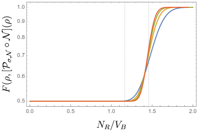
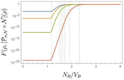
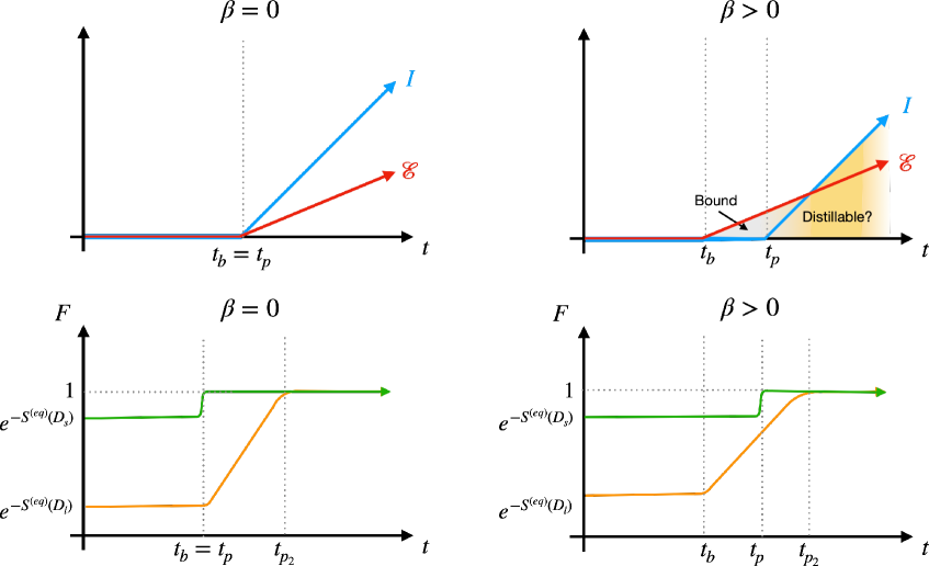
Figure 1: Top row: The general behavior of logarithmic negativity (red) and mutual information (blue) is shown for finite temperature equilibrated pure states, specifically evaporating black holes. While the mutual information within the radiation does not become extensive until the Page time tpsubscript𝑡𝑝t_{p}, the negativity starts to become extensive at the earlier time tbsubscript𝑡𝑏t_{b}, signaling the existence of quantum correlations in the radiation prior to the Page time that cannot be distilled into EPR pairs. After the Page time, we expect the entanglement to be distillable but do not have a rigorous proof. Bottom row: We also plot the fidelity of the Petz map in the Hayden-Preskill experiment for small (green) and large (orange) diaries. For small diaries, the fidelity increases rapidly from its initial value to 1 at tpsubscript𝑡𝑝t_{p}. For sufficiently large diaries, the fidelity begins to increase at the time scale tb<tpsubscript𝑡𝑏subscript𝑡𝑝t_{b}<t_{p}, and reaches a value close to 1 at tp2>tpsubscript𝑡subscript𝑝2subscript𝑡𝑝t_{p_{2}}>t_{p}. tp2subscript𝑡subscript𝑝2t_{p_{2}} is defined as the time when the entropy of the radiation is equal to the entropy of the black hole plus the equilibrium entropy of the diary. The cartoon plots in the bottom row are schematic, but should be thought to have a logarithmically scaled y-axis.

Our main results can be summarized as follows:111Some of the results in the first point below have been summarized in an earlier paper [6].

  1. 1.

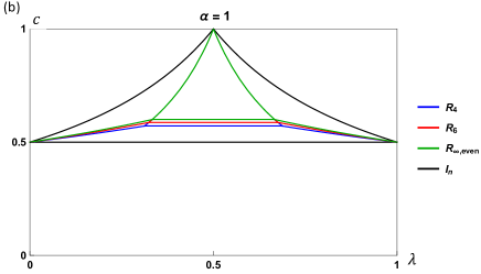
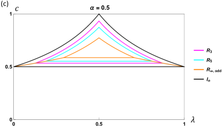
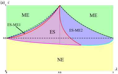
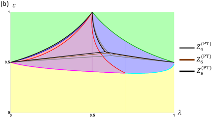
    Consider a system AB𝐴𝐵AB in a macroscopically equilibrated pure state |ΨketΨ\ket{\Psi}, and a subsystem A=A1A2𝐴subscript𝐴1subscript𝐴2A=A_{1}\cup A_{2} whose reduced density operator is given by ρA=TrB|ΨΨ|subscript𝜌𝐴subscriptTr𝐵ketΨbraΨ\rho_{A}=\text{Tr}_{B}\ket{\Psi}\bra{\Psi}. We study the Renyi negativities Rn(A1,A2)subscript𝑅𝑛subscript𝐴1subscript𝐴2R_{n}(A_{1},A_{2}) and the logarithmic negativity (A1,A2)subscript𝐴1subscript𝐴2{{\mathcal{E}}}(A_{1},A_{2}), which encode bi-partite entanglement between A1subscript𝐴1A_{1} and A2subscript𝐴2A_{2} in the mixed state ρAsubscript𝜌𝐴\rho_{A}. The logarithmic negativity {{\mathcal{E}}} is non-zero only if ρAsubscript𝜌𝐴\rho_{A} is not separable, and can be used to lower-bound the PPT entanglement cost, (A1,A2)Ec(ppt,exact)(A1,A2)subscript𝐴1subscript𝐴2superscriptsubscript𝐸𝑐pptexactsubscript𝐴1subscript𝐴2\mathcal{E}(A_{1},A_{2})\leq E_{c}^{\rm(ppt,exact)}(A_{1},A_{2}) [7]. Depending on the sizes of A𝐴A and A1subscript𝐴1A_{1}, the behaviors of the negativities give rise to an intricate phase diagram, exhibiting a rich entanglement structure. In particular, finite temperature has a significant effect on the qualitative structure of the entanglement phase diagram.

    The behavior of the negativities can further be contrasted with that of the Renyi mutual informations In(A1,A2)subscript𝐼𝑛subscript𝐴1subscript𝐴2I_{n}(A_{1},A_{2}) and the mutual information I(A1,A2)𝐼subscript𝐴1subscript𝐴2I(A_{1},A_{2}) between A1subscript𝐴1A_{1} and A2subscript𝐴2A_{2}. Unlike the logarithmic negativity, the mutual information I𝐼I can contain information about both classical and quantum correlations in the state, but is nevertheless of importance for understanding the entanglement structure as it upper-bounds the distillable entanglement, Ed(A1,A2)12I(A1,A2)subscript𝐸𝑑subscript𝐴1subscript𝐴212𝐼subscript𝐴1subscript𝐴2E_{d}(A_{1},A_{2})\leq{{\frac{1}{2}}}I(A_{1},A_{2}) [8]. The phase structure indicated by the mutual information I(A1,A2)𝐼subscript𝐴1subscript𝐴2I(A_{1},A_{2}) appears to be insensitive to finite temperature, although the Renyi mutual informations can be sensitive to finite temperature. Comparison between (Renyi) mutual information and negativities indicate that these quantities likely capture complementary aspects of mixed state entanglement.

    A particularly surprising result is that in the thermodynamic limit, there can be a finite region in the entanglement phase diagram where the logarithmic negativity is extensive, but the mutual information is sub-extensive, implying that there is a large amount of bound entanglement. This phenomenon does not take place in the infinite temperature case previously studied in [9]. This observation also has important implications for black hole physics. It implies the existence of a new time scale tbsubscript𝑡𝑏t_{b} before the Page time tpsubscript𝑡𝑝t_{p}, after which there is already a significant amount of entanglement correlation within the Hawking radiation. In the following point, we give an operational interpretation of tbsubscript𝑡𝑏t_{b}. See Fig. 1.

    These results on the behavior of the negativity and mutual information, together with the behavior of a quantity called reflected entropy, also suggest the existence of nontrivial multi-partite entanglement among different parts of the radiation and the black hole.

  2. 2.

    We consider the Hayden-Preskill thought experiment [10]222Throw a diary into an evaporating black hole, and see when the information of the diary is recoverable from the radiation. for information transfer from a black hole to its Hawking radiation at a finite temperature. We take two perspectives on this process of information transfer, viewing it as (i) growth of the mutual information between an auxiliary reference system and the radiation subsystem, as in [10]; (ii) growth of the fidelity of a recovery map for extracting the information from the radiation. The recovery map is in turn studied from two approaches: from a lower bound on its fidelity provided by relative entropy, and from a direct calculation of the fidelity of an explicit map called the Petz map. We show that in both approaches, the results at finite temperature can be expressed in terms of natural quantum information-theoretic measures of the thermal state. In particular, for a “small” diary whose size does not scale with the total volume of the system, the fidelity rapidly grows from its initial small value to its maximum value of 1 at the standard Page time tpsubscript𝑡𝑝t_{p}. For a “large” diary whose size does scale with the volume, the fidelity becomes exponentially close to 1 at a time tp2>tpsubscript𝑡subscript𝑝2subscript𝑡𝑝t_{p_{2}}>t_{p}, which was previously identified in [11]. But intriguingly, the fidelity of the large diary first starts to grow from its small initial value at the same time scale tb<tpsubscript𝑡𝑏subscript𝑡𝑝t_{b}<t_{p} when the logarithmic negativity between parts of the radiation starts to grow.333As we vary the size of the diary from O(1)𝑂1O(1) to O(V)𝑂𝑉O(V) where V𝑉V is the volume of the system, the time scale for the beginning of fidelity growth gradually changes from tpsubscript𝑡𝑝t_{p} to tbsubscript𝑡𝑏t_{b}. This result is in contrast to the prior literature based mostly on infinite temperature calculations, which always took tpsubscript𝑡𝑝t_{p} and tp2subscript𝑡subscript𝑝2t_{p_{2}} to be the only relevant time scales for information recovery. These statements can be viewed as giving operational definitions of the time scales tbsubscript𝑡𝑏t_{b}, tpsubscript𝑡𝑝t_{p}, and tp2subscript𝑡subscript𝑝2t_{p_{2}}, which apply both at infinite temperature and finite temperature. See Fig. 1.

The plan of the paper is as follows. In Section 2, we review some relevant concepts about mixed-state entanglement, the Renyi and logarithmic negativities, and the Petz recovery map, as well as the equilibrium approximation developed in [1]. In Section 3, we explain how to generalize the equilibrium approximation to the various information-theoretic quantities studied in this paper. In Section 4, we use these methods to find entanglement phase diagrams for a variety of universality classes of thermalized states. Section 5 discusses the operational implications of these entanglement phase diagrams, and the consequences for black hole dynamics. We study the question of information recovery from the radiation of an evaporating black hole at finite temperature in Section 6, and conclude with some discussion of future directions in Section 7. Many details are relegated to appendices.

2 Review of background materials

In this section we review topics and technical tools that will be used in subsequent discussions.

2.1 Entanglement in mixed states

Consider a state ρ𝜌\rho in a bipartite system A=A1A2subscript𝐴tensor-productsubscriptsubscript𝐴1subscriptsubscript𝐴2{{\mathcal{H}}}_{A}={{\mathcal{H}}}_{A_{1}}\otimes{{\mathcal{H}}}_{A_{2}}. ρ𝜌\rho is said to be a separable state if it can be written as a convex combination of product states,

ρ=i=1qpi(ρi)A1(ρ~i)A2,0pa1,a=1qpa=1.formulae-sequenceformulae-sequence𝜌superscriptsubscript𝑖1𝑞tensor-productsubscript𝑝𝑖subscriptsubscript𝜌𝑖subscript𝐴1subscriptsubscript~𝜌𝑖subscript𝐴20subscript𝑝𝑎1superscriptsubscript𝑎1𝑞subscript𝑝𝑎1\rho=\sum_{i=1}^{q}p_{i}\,(\rho_{i})_{A_{1}}\otimes(\tilde{\rho}_{i})_{A_{2}}\,,\quad 0\leq p_{a}\leq 1,\quad\sum_{a=1}^{q}p_{a}=1\,. (2.1)

Such a state has no quantum entanglement, as the correlations in it can be given a classical hidden-variable description [12], and it can be prepared using only local operations and classical communications (LOCC) without any need for EPR pairs between A1subscript𝐴1A_{1} and A2subscript𝐴2A_{2}. Any state that is not separable is said to be entangled.

If we know that ρ𝜌\rho is a pure state, then its entanglement entropy or von Neumann entropy in A1subscript𝐴1A_{1}, defined as

SA1(ρ):=Tr[ρA1logρA1],ρA1:=TrA2[ρ]formulae-sequenceassignsubscript𝑆subscript𝐴1𝜌Trdelimited-[]subscript𝜌subscript𝐴1subscript𝜌subscript𝐴1assignsubscript𝜌subscript𝐴1subscriptTrsubscript𝐴2delimited-[]𝜌S_{A_{1}}(\rho):=-\text{Tr}[\rho_{A_{1}}\log\rho_{A_{1}}],\quad\rho_{A_{1}}:=\text{Tr}_{A_{2}}[\rho] (2.2)

is sufficient to determine whether it is separable or entangled. ρ𝜌\rho is an entangled state if SA1(ρ)subscript𝑆subscript𝐴1𝜌S_{A_{1}}(\rho) is non-zero, and a separable state with q=1𝑞1q=1 otherwise.

If ρ𝜌\rho is not a pure state, then no easily calculable quantity is known which is zero when the state is unentangled and non-zero when it is entangled. In fact, it is an NP-hard problem to determine whether an arbitrary state is entangled [13].

One familiar quantity that captures correlations between regions A1subscript𝐴1A_{1} and A2subscript𝐴2A_{2} in the state ρ𝜌\rho is the mutual information,

I(A1,A2):=SA1(ρ)+SA2(ρ)SA(ρ),assign𝐼subscript𝐴1subscript𝐴2subscript𝑆subscript𝐴1𝜌subscript𝑆subscript𝐴2𝜌subscript𝑆𝐴𝜌I(A_{1},A_{2}):=S_{A_{1}}(\rho)+S_{A_{2}}(\rho)-S_{A}(\rho), (2.3)

where SAi(ρ)subscript𝑆subscript𝐴𝑖𝜌S_{A_{i}}(\rho) is the von Neumann entropy defined in (2.2). While the mutual information is non-zero for any entangled state, it is also nonzero for a separable state as in (2.1) with q>1𝑞1q>1, and can hence reflect both classical correlations and quantum entanglement.

Another useful quantity for studying entanglement in mixed states is the logarithmic negativity. Suppose the density matrix ρ𝜌\rho has matrix elements ρa1a2,b1b2subscript𝜌subscript𝑎1subscript𝑎2subscript𝑏1subscript𝑏2\rho_{a_{1}a_{2},b_{1}b_{2}} in some basis |a1a2ketsubscript𝑎1subscript𝑎2\ket{a_{1}a_{2}} for A1A2tensor-productsubscriptsubscript𝐴1subscriptsubscript𝐴2{{\mathcal{H}}}_{A_{1}}\otimes{{\mathcal{H}}}_{A_{2}}. We define the partial transpose ρT2superscript𝜌subscript𝑇2\rho^{T_{2}} of ρ𝜌\rho with respect to A2subscriptsubscript𝐴2{{\mathcal{H}}}_{A_{2}} as

ρa1a2,b1b2T2:=ρa1b2,b1a2.assignsubscriptsuperscript𝜌subscript𝑇2subscript𝑎1subscript𝑎2subscript𝑏1subscript𝑏2subscript𝜌subscript𝑎1subscript𝑏2subscript𝑏1subscript𝑎2\rho^{T_{2}}_{a_{1}a_{2},b_{1}b_{2}}:=\rho_{a_{1}b_{2},b_{1}a_{2}}\ . (2.4)

The eigenvalues of ρT2superscript𝜌subscript𝑇2\rho^{T_{2}} can now in principle be negative. The presence of negative eigenvalues in ρT2superscript𝜌subscript𝑇2\rho^{T_{2}} reflects that subsystems A1subscript𝐴1A_{1} and A2subscript𝐴2A_{2} are entangled; for a separable state (2.1), ρT2=i=1qpi(ρi)A1(ρ~i)A2Tsuperscript𝜌subscript𝑇2superscriptsubscript𝑖1𝑞tensor-productsubscript𝑝𝑖subscriptsubscript𝜌𝑖subscript𝐴1subscriptsuperscriptsubscript~𝜌𝑖𝑇subscript𝐴2\rho^{T_{2}}=\sum_{i=1}^{q}p_{i}\,(\rho_{i})_{A_{1}}\otimes(\tilde{\rho}_{i})^{T}_{A_{2}} remains a legitimate density operator with non-negative eigenvalues, as the transpose of a positive operator is still positive. This motivates one to define the logarithmic negativity as444ρT1superscript𝜌subscript𝑇1\rho^{T_{1}} has the same eigenvalues as ρT2superscript𝜌subscript𝑇2\rho^{T_{2}}, and thus the definition of {{\mathcal{E}}} is symmetric between A1subscript𝐴1A_{1} and A2subscript𝐴2A_{2}. [14, 15, 16, 17, 18, 19, 20]

(A1,A2):=logk|λk|,{{\mathcal{E}}}(A_{1},A_{2}):=\log\sum_{k}|\lambda_{k}|, (2.5)

where λksubscript𝜆𝑘\lambda_{k} are the eigenvalues of ρT2superscript𝜌subscript𝑇2\rho^{T_{2}}. By definition, ρT2superscript𝜌subscript𝑇2\rho^{T_{2}} has unit trace, and thus k|λk|1subscript𝑘subscript𝜆𝑘1\sum_{k}|\lambda_{k}|\geq 1, which implies that 00{{\mathcal{E}}}\geq 0. States with =00{{\mathcal{E}}}=0 are referred to as positive partial transpose (PPT) states, and could still be entangled. Separable states form a proper subset of PPT states. Hence, unlike non-zero mutual information, a non-zero value of the logarithmic negativity implies that ρ𝜌\rho is entangled.

Another natural way to quantify entanglement is through hypothetical protocols for interconversion between the state ρ𝜌\rho and some number of EPR pairs shared between A1subscript𝐴1A_{1} and A2subscript𝐴2A_{2}, using only LOCC. This leads to two operationally motivated measures of entanglement, known as the entanglement cost Ecsubscript𝐸𝑐E_{c} and the distillable entanglement Edsubscript𝐸𝑑E_{d} [21].

To define both of the above quantities, suppose we take n𝑛n copies of the original system, A1nA2ntensor-productsuperscriptsubscript𝐴1tensor-productabsent𝑛superscriptsubscript𝐴2tensor-productabsent𝑛A_{1}^{\otimes n}\otimes A_{2}^{\otimes n}. We allow only local operations and classical communication between A1nsuperscriptsubscript𝐴1tensor-productabsent𝑛A_{1}^{\otimes n} and A2nsuperscriptsubscript𝐴2tensor-productabsent𝑛A_{2}^{\otimes n}, and consider conversions between ρnsuperscript𝜌tensor-productabsent𝑛\rho^{\otimes n} and (|EPREPR|)msuperscriptketEPRbraEPRtensor-productabsentm(\ket{\rm EPR}\bra{\rm EPR})^{\otimes m}, where

|EPR=12(|0x1|0x2+|1x1|1x2),x1,x2 are qubits in A1n,A2n.ketEPR12subscriptket0subscriptx1subscriptket0subscriptx2subscriptket1subscriptx1subscriptket1subscriptx2subscriptx1subscriptx2 are qubits in A1n,A2n.\ket{\rm EPR}=\frac{1}{\sqrt{2}}(\ket{0}_{x_{1}}\ket{0}_{x_{2}}+\ket{1}_{x_{1}}\ket{1}_{x_{2}}),\quad x_{1},x_{2}\text{ are qubits in $A_{1}^{\otimes n},A_{2}^{\otimes n}$.} (2.6)

First consider the conversion from (|EPREPR|)msuperscriptketEPRbraEPRtensor-productabsentm(\ket{\rm EPR}\bra{\rm EPR})^{\otimes m} to ρnsuperscript𝜌tensor-productabsent𝑛\rho^{\otimes n} under different choices {{\mathcal{L}}} of LOCC operations, with vanishing error in the limit n𝑛n\rightarrow\infty. The entanglement cost Ecsubscript𝐸𝑐E_{c} is defined as the minimum ratio mn𝑚𝑛\frac{m}{n} over all choices of {{\mathcal{L}}} [22]. Next, consider the conversion from ρnsuperscript𝜌tensor-productabsent𝑛\rho^{\otimes n} to (|EPREPR|)msuperscriptketEPRbraEPRtensor-productabsentm(\ket{\rm EPR}\bra{\rm EPR})^{\otimes m} under LOCC operations {{\mathcal{L}}}, with vanishing error in the limit n𝑛n\rightarrow\infty. Now the maximum ratio mn𝑚𝑛\frac{m}{n} over all choices of {{\mathcal{L}}} is defined as the distillable entanglement Edsubscript𝐸𝑑E_{d}.

For a pure state ρ𝜌\rho, Ecsubscript𝐸𝑐E_{c} and Edsubscript𝐸𝑑E_{d} are both equal to the entanglement entropy S(ρA1)𝑆subscript𝜌subscript𝐴1S(\rho_{A_{1}}) [23]. This is another justification for seeing the entanglement entropy as a natural measure of entanglement for pure states. For mixed states, in general EcEdsubscript𝐸𝑐subscript𝐸𝑑E_{c}\geq E_{d}, and neither of these quantities must be equal to S(A1)(ρ)superscript𝑆subscript𝐴1𝜌S^{(A_{1})}(\rho) [21]. In fact, there can be “bound-entangled” states, for which Ecsubscript𝐸𝑐E_{c} is non-zero while Ed=0subscript𝐸𝑑0E_{d}=0 [24].

We can also consider replacing the LOCC operations of the above definitions with a larger set of operations called PPT-preserving transformations, which send any state σ𝜎\sigma with σT20superscript𝜎subscript𝑇20\sigma^{T_{2}}\geq 0 to another state σsuperscript𝜎\sigma^{\prime} with (σ)T20superscriptsuperscript𝜎subscript𝑇20(\sigma^{\prime})^{T_{2}}\geq 0. The entanglement cost and distillable entanglement under such operations, Ec(ppt)superscriptsubscript𝐸𝑐pptE_{c}^{(\rm ppt)} and Ed(ppt)superscriptsubscript𝐸𝑑pptE_{d}^{(\rm ppt)}, are then natural generalizations of the definitions for LOCC given above.

Since LOCC operations are a proper subset of PPT-preserving operations, it is clear that Ec(ppt)Ecsuperscriptsubscript𝐸𝑐pptsubscript𝐸𝑐E_{c}^{(\rm ppt)}\leq E_{c}, and Ed(ppt)Edsuperscriptsubscript𝐸𝑑pptsubscript𝐸𝑑E_{d}^{(\rm ppt)}\geq E_{d}. It turns out that it is not possible to find states where Ec(ppt)superscriptsubscript𝐸𝑐pptE_{c}^{\rm(ppt)} is non-zero while Ed(ppt)=0superscriptsubscript𝐸𝑑ppt0E_{d}^{\rm(ppt)}=0 [25]. However, there are known examples of states for which the preparation by PPT operations is irreversible, i.e. Ec(ppt)>Ed(ppt)superscriptsubscript𝐸𝑐pptsuperscriptsubscript𝐸𝑑pptE_{c}^{\rm(ppt)}>E_{d}^{\rm(ppt)} [26].

In the discussion below, we will sometimes refer to “exact” versions of each of the above entanglement costs and distillable entanglements. For these quantities, we modify the above definitions by requiring that the error in the conversion vanishes before taking the n𝑛n\rightarrow\infty limit. For example, Ec(exact)superscriptsubscript𝐸𝑐exactE_{c}^{\rm(exact)} refers to the minimum ratio mn𝑚𝑛\frac{m}{n} in the exact conversion from (|EPREPR|)msuperscriptketEPRbraEPRtensor-productabsentm(\ket{\rm EPR}\bra{\rm EPR})^{\otimes m} to ρnsuperscript𝜌tensor-productabsent𝑛\rho^{\otimes n} by LOCC in the n𝑛n\rightarrow\infty limit. Ed(exact)superscriptsubscript𝐸𝑑exactE_{d}^{\rm(exact)}, Ec(ppt,exact)superscriptsubscript𝐸𝑐pptexactE_{c}^{(\rm ppt,exact)}, and Ed(ppt,exact)superscriptsubscript𝐸𝑑pptexactE_{d}^{(\rm ppt,exact)} are defined similarly. It is then clear, for instance, that Ec(exact)Ecsuperscriptsubscript𝐸𝑐exactsubscript𝐸𝑐E_{c}^{\rm(exact)}\geq E_{c}, and Ed(ppt,exact)Ed(ppt)superscriptsubscript𝐸𝑑pptexactsuperscriptsubscript𝐸𝑑pptE_{d}^{\rm(ppt,exact)}\leq E_{d}^{\rm(ppt)}.

While the entanglement cost and the distillable entanglement for mixed states are natural generalizations of the entanglement entropy for pure states from an operational perspective, these measures are difficult to compute in practice even for few-qubit systems. However, they can be related to computable measures such as logarithmic negativity and mutual information through upper and lower bounds. Two inequalities which will be useful in our subsequent discussion are a relation between the mutual information and the distillable entanglement [8],

Ed(A1,A2)12I(A1,A2),subscript𝐸𝑑subscript𝐴1subscript𝐴212𝐼subscript𝐴1subscript𝐴2E_{d}(A_{1},A_{2})\leq{{\frac{1}{2}}}I(A_{1},A_{2})\,, (2.7)

and a relation between the logarithmic negativity and the exact PPT entanglement cost [7],

(A1,A2)Ec(ppt,exact)(A1,A2)Ec(exact)(A1,A2).subscript𝐴1subscript𝐴2superscriptsubscript𝐸𝑐pptexactsubscript𝐴1subscript𝐴2superscriptsubscript𝐸𝑐exactsubscript𝐴1subscript𝐴2\mathcal{E}(A_{1},A_{2})\leq E_{c}^{\rm(ppt,exact)}(A_{1},A_{2})\leq E_{c}^{\rm(exact)}(A_{1},A_{2})\,. (2.8)

2.2 Renyi entropies and negativities

Recall that in order to calculate the von Neumann entropy, it is often useful to introduce higher moments of the reduced density matrix, which we will refer to as Renyi partition functions,

𝒵n,A=Tr[(ρA)n].subscript𝒵𝑛𝐴Trdelimited-[]superscriptsubscript𝜌𝐴𝑛{\mathcal{Z}}_{n,A}=\text{Tr}[(\rho_{A})^{n}]. (2.9)

These partition functions can be used to define the n𝑛n-th Renyi entropies

Sn,A(ρ)=1n1log𝒵n,A,subscript𝑆𝑛𝐴𝜌1𝑛1subscript𝒵𝑛𝐴S_{n,A}(\rho)=-\frac{1}{n-1}\log{\mathcal{Z}}_{n,A}, (2.10)

which can in turn be used to define the n𝑛n-th Renyi mutual informations

In(A1,A2)=Sn,A1+Sn,A2Sn,A.subscript𝐼𝑛subscript𝐴1subscript𝐴2subscript𝑆𝑛subscript𝐴1subscript𝑆𝑛subscript𝐴2subscript𝑆𝑛𝐴I_{n}(A_{1},A_{2})=S_{n,A_{1}}+S_{n,A_{2}}-S_{n,A}\,. (2.11)

The Renyi entropies and mutual informations provide further information about the entanglement structure in addition to the von Neumann entropy and mutual information; however, note that in some cases the Renyi mutual information can be negative, unlike the mutual information, which is one reason why the Renyi mutual information should only be considered as proxies for correlation measures. The von Neumann entropy can be written as a limit of the Renyi entropies in the index n𝑛n,

SA=limn1Sn,A.subscript𝑆𝐴subscript𝑛1subscript𝑆𝑛𝐴S_{A}=\lim_{n\rightarrow 1}S_{n,A}\,. (2.12)

In some cases, such as when the Sn,Asubscript𝑆𝑛𝐴S_{n,A} cannot be written as an analytic function of n𝑛n, we may not be able to use analytic continuation to find the von Neumann entropy. Another method for obtaining the von Neumann entropy using the Renyi partition functions that turns out to be more generally applicable is through a quantity known as the resolvent,

(λ)=Tr(1λ𝟏ρA)=1λn=01λn𝒵n,A,𝜆Tr1𝜆1subscript𝜌𝐴1𝜆superscriptsubscript𝑛01superscript𝜆𝑛subscript𝒵𝑛𝐴{\mathcal{R}}(\lambda)=\text{Tr}\left(\frac{1}{\lambda\mathbf{1}-\rho_{A}}\right)=\frac{1}{\lambda}\sum_{n=0}^{\infty}\frac{1}{\lambda^{n}}{\mathcal{Z}}_{n,A}, (2.13)

where we take λ𝜆\lambda to be a general complex parameter. Since the spectrum of ρAsubscript𝜌𝐴\rho_{A} is bounded, the power series in the second equality is convergent for sufficiently large |λ|𝜆|\lambda|. We can then compute (λ)𝜆{\mathcal{R}}(\lambda) for such λ𝜆\lambda’s and then analytically continue to obtain other values of λ𝜆\lambda. The density of eigenvalues of ρAsubscript𝜌𝐴\rho_{A}, known as the entanglement spectrum, can be obtained from the discontinuities of (λ)𝜆{\mathcal{R}}(\lambda) across the real axis,

D(λ)=1πIm(λiϵ),λ.formulae-sequence𝐷𝜆1𝜋Im𝜆𝑖italic-ϵ𝜆D(\lambda)=\frac{1}{\pi}{\rm Im}\,{\mathcal{R}}(\lambda-i\epsilon),\quad\lambda\in{\mathbb{{R}}}\ . (2.14)

We can then use D(λ)𝐷𝜆D(\lambda) to calculate the von Neumann entropy,

SA=𝑑λD(λ)λlogλ.subscript𝑆𝐴differential-d𝜆𝐷𝜆𝜆𝜆S_{A}=-\int d\lambda\,D(\lambda)\,\lambda\log\lambda\ . (2.15)

It is similarly useful to define the higher moments of the partially transposed density matrix ρAT2superscriptsubscript𝜌𝐴subscript𝑇2\rho_{A}^{T_{2}} introduced in (2.4), which we refer to as partial transpose partition functions,

𝒵n(PT)=Tr(ρAT2)n.superscriptsubscript𝒵𝑛PTTrsuperscriptsuperscriptsubscript𝜌𝐴subscript𝑇2𝑛{\mathcal{Z}}_{n}^{(\rm PT)}=\text{Tr}\left(\rho_{A}^{T_{2}}\right)^{n}\ . (2.16)

By definition 𝒵1(PT)=1superscriptsubscript𝒵1PT1{\mathcal{Z}}_{1}^{(\rm PT)}=1, and it can be readily checked that 𝒵2(PT)=Trρ2superscriptsubscript𝒵2PTTrsuperscript𝜌2{\mathcal{Z}}_{2}^{(\rm PT)}=\text{Tr}\rho^{2}, so nontrivial moments start with n=3𝑛3n=3. There are qualitative differences between even and odd n𝑛n’s, as

𝒵2m(PT)=λi>0|λi|2m+λi<0|λi|2m,𝒵2m+1(PT)=λi>0|λi|2m+1λi<0|λi|2m+1.formulae-sequencesuperscriptsubscript𝒵2𝑚PTsubscriptsubscript𝜆𝑖0superscriptsubscript𝜆𝑖2𝑚subscriptsubscript𝜆𝑖0superscriptsubscript𝜆𝑖2𝑚superscriptsubscript𝒵2𝑚1PTsubscriptsubscript𝜆𝑖0superscriptsubscript𝜆𝑖2𝑚1subscriptsubscript𝜆𝑖0superscriptsubscript𝜆𝑖2𝑚1{\mathcal{Z}}_{2m}^{(\rm PT)}=\sum_{\lambda_{i}>0}\left|\lambda_{i}\right|^{2m}+\sum_{\lambda_{i}<0}\left|\lambda_{i}\right|^{2m},\qquad{\mathcal{Z}}_{2m+1}^{(\rm PT)}=\sum_{\lambda_{i}>0}\left|\lambda_{i}\right|^{2m+1}-\sum_{\lambda_{i}<0}\left|\lambda_{i}\right|^{2m+1}\ . (2.17)

The logarithmic negativity {{\mathcal{E}}} can be obtained by analytically continuing 𝒵2m(PT)superscriptsubscript𝒵2𝑚PT{\mathcal{Z}}_{2m}^{(\rm PT)} as

=limm12log𝒵2m(PT).subscript𝑚12superscriptsubscript𝒵2𝑚PT\mathcal{E}=\lim_{m\rightarrow{{\frac{1}{2}}}}\log{\mathcal{Z}}_{2m}^{(\rm PT)}\ . (2.18)

It can be shown that a PPT state satisfies [27]

𝒵3(PT)(𝒵2(PT))2.superscriptsubscript𝒵3PTsuperscriptsuperscriptsubscript𝒵2PT2{\mathcal{Z}}_{3}^{(\rm PT)}\geq\left({\mathcal{Z}}_{2}^{(\rm PT)}\right)^{2}\ . (2.19)

Thus if 𝒵3(PT)<(𝒵2(PT))2superscriptsubscript𝒵3PTsuperscriptsuperscriptsubscript𝒵2PT2{\mathcal{Z}}_{3}^{(\rm PT)}<\left({\mathcal{Z}}_{2}^{(\rm PT)}\right)^{2}, then it must be that >00{{\mathcal{E}}}>0, which provides a quick diagnostic. The condition (2.19) is weaker than the PPT condition; there can be states that satisfy (2.19) but still have >00{{\mathcal{E}}}>0.

We can also use the partial transpose partition functions to define quantities called the n𝑛n-th Renyi negativities,

Rn(A1,A2)=bnlog[𝒵n(PT)𝒵n,A],bn={11nnodd12nneven.formulae-sequencesubscript𝑅𝑛subscript𝐴1subscript𝐴2subscript𝑏𝑛superscriptsubscript𝒵𝑛PTsubscript𝒵𝑛𝐴subscript𝑏𝑛cases11𝑛𝑛odd12𝑛𝑛evenR_{n}(A_{1},A_{2})=b_{n}\log\left[{{\mathcal{Z}}_{n}^{(\rm PT)}\over{\mathcal{Z}}_{n,A}}\right],\quad b_{n}=\begin{cases}{1\over 1-n}&n\,{\rm odd}\cr{1\over 2-n}&n\,{\rm even}\end{cases}\ . (2.20)

n=1,2𝑛12n=1,2 should be understood as being defined through limits. More explicitly,

R1=λi>0|λi|log|λi|+λi<0|λi|log|λi|SA(ρ),subscript𝑅1subscriptsubscript𝜆𝑖0subscript𝜆𝑖subscript𝜆𝑖subscriptsubscript𝜆𝑖0subscript𝜆𝑖subscript𝜆𝑖subscript𝑆𝐴𝜌\displaystyle R_{1}=-\sum_{\lambda_{i}>0}|\lambda_{i}|\log|\lambda_{i}|+\sum_{\lambda_{i}<0}|\lambda_{i}|\log|\lambda_{i}|-S_{A}(\rho), (2.21)
R2=1𝒵2(i|λi|2log|λi|+i|λ~i|2logλ~i),subscript𝑅21subscript𝒵2subscript𝑖superscriptsubscript𝜆𝑖2subscript𝜆𝑖subscript𝑖superscriptsubscript~𝜆𝑖2subscript~𝜆𝑖\displaystyle R_{2}={1\over{\mathcal{Z}}_{2}}\left(-\sum_{i}|\lambda_{i}|^{2}\log|\lambda_{i}|+\sum_{i}|\tilde{\lambda}_{i}|^{2}\log\tilde{\lambda}_{i}\right), (2.22)

where λ~isubscript~𝜆𝑖\tilde{\lambda}_{i} are eigenvalues of ρ𝜌\rho. The logarithmic negativity can also be obtained from R2msubscript𝑅2𝑚R_{2m} by analytic continuation

=limm12R2m.subscript𝑚12subscript𝑅2𝑚{{\mathcal{E}}}=\lim_{m\to{{\frac{1}{2}}}}R_{2m}\ . (2.23)

For a product state ρ=ρA1ρA2𝜌tensor-productsubscript𝜌subscript𝐴1subscript𝜌subscript𝐴2\rho=\rho_{A_{1}}\otimes\rho_{A_{2}}, we have 𝒵n(PT)=𝒵nsuperscriptsubscript𝒵𝑛PTsubscript𝒵𝑛{\mathcal{Z}}_{n}^{(\rm PT)}={\mathcal{Z}}_{n} and thus Rn=0subscript𝑅𝑛0R_{n}=0. But for a general separable state, Rnsubscript𝑅𝑛R_{n} are in general nonzero. Thus from nonzero Rnsubscript𝑅𝑛R_{n}, we cannot conclude for certain that there is nonzero entanglement. Even so, there are indications that the Renyi negativities often have the same general behavior as the logarithmic negativity, and these quantities have proven useful in a variety of problems [28, 29, 30, 31, 32, 33, 34, 35].

It is often useful to compare the Renyi negativities with the Renyi mutual informations defined in (2.11). In fact, when ρ𝜌\rho is a pure state, the Renyi negativities and Renyi mutual informations are related in a simple way. More explicitly, in this case we have

R2m(A1,A2)=Sm,A1=12Im(A1,A2),subscript𝑅2𝑚subscript𝐴1subscript𝐴2subscript𝑆𝑚subscript𝐴112subscript𝐼𝑚subscript𝐴1subscript𝐴2\displaystyle R_{2m}(A_{1},A_{2})=S_{m,A_{1}}={{\frac{1}{2}}}I_{m}(A_{1},A_{2}), (2.24)
R2m+1(A1,A2)=S2m+1,A1=12I2m+1(A1,A2).subscript𝑅2𝑚1subscript𝐴1subscript𝐴2subscript𝑆2𝑚1subscript𝐴112subscript𝐼2𝑚1subscript𝐴1subscript𝐴2\displaystyle R_{2m+1}(A_{1},A_{2})=S_{2m+1,A_{1}}={{\frac{1}{2}}}I_{2m+1}(A_{1},A_{2})\ . (2.25)

We also have

(A1,A2)=S12,A1=12I12(A1,A2).subscript𝐴1subscript𝐴2subscript𝑆12subscript𝐴112subscript𝐼12subscript𝐴1subscript𝐴2{{\mathcal{E}}}(A_{1},A_{2})=S_{{{\frac{1}{2}}},A_{1}}={{\frac{1}{2}}}I_{{{\frac{1}{2}}}}(A_{1},A_{2})\ . (2.26)

Equation (2.26) gives a rough intuition on the relative normalization between the logarithmic negativity and mutual information.

In some cases, we will find that the 𝒵n(PT)superscriptsubscript𝒵𝑛PT{\mathcal{Z}}_{n}^{\rm(PT)} and Rnsubscript𝑅𝑛R_{n} cannot be written simply as analytic functions of n𝑛n, so that we will not be able to use (2.18) or (2.23) to find {{\mathcal{E}}}. Again, a more generally applicable method is to use the resolvent for ρAT2superscriptsubscript𝜌𝐴subscript𝑇2\rho_{A}^{T_{2}}:

RN(λ)=Tr(1λ𝟏ρAT2)=1λn=01λn𝒵n(PT).subscript𝑅𝑁𝜆Tr1𝜆1superscriptsubscript𝜌𝐴subscript𝑇21𝜆superscriptsubscript𝑛01superscript𝜆𝑛superscriptsubscript𝒵𝑛PTR_{N}(\lambda)=\text{Tr}\left(\frac{1}{\lambda\mathbf{1}-\rho_{A}^{T_{2}}}\right)=\frac{1}{\lambda}\sum_{n=0}^{\infty}\frac{1}{\lambda^{n}}{\mathcal{Z}}_{n}^{\rm(PT)}\ . (2.27)

The density of eigenvalues of ρAT2superscriptsubscript𝜌𝐴subscript𝑇2\rho_{A}^{T_{2}}, known as the negativity spectrum, can be obtained from the discontinuities of RN(λ)subscript𝑅𝑁𝜆R_{N}(\lambda) across the real axis,

DN(λ)=1πImRN(λiϵ),λ,formulae-sequencesubscript𝐷𝑁𝜆1𝜋Imsubscript𝑅𝑁𝜆𝑖italic-ϵ𝜆D_{N}(\lambda)=\frac{1}{\pi}{\rm Im}\,R_{N}(\lambda-i\epsilon),\quad\lambda\in{\mathbb{{R}}}\ , (2.28)

and we can use DN(λ)subscript𝐷𝑁𝜆D_{N}(\lambda) to calculate the logarithmic negativity,

(A1,A2)=log(𝑑λDN(λ)|λ|).subscript𝐴1subscript𝐴2differential-d𝜆subscript𝐷𝑁𝜆𝜆{{\mathcal{E}}}(A_{1},A_{2})=\log\left(\int d\lambda\,D_{N}(\lambda)\,|\lambda|\right)\ . (2.29)

2.3 Brief review of the equilibrium approximation

In this subsection, we review the equilibrium approximation introduced in [1], which will be the main tool we use in this paper. We first discuss the formulation for a pure state, and then for a mixed state.

2.3.1 Pure states

We consider a system evolving from a far-from-equilibrium pure state ρ0=|Ψ0Ψ0|subscript𝜌0ketsubscriptΨ0brasubscriptΨ0\rho_{0}=\ket{\Psi_{0}}\bra{\Psi_{0}} to a state ρ=|ΨΨ|𝜌ketΨbraΨ\rho=\ket{\Psi}\bra{\Psi} with |Ψ=U|Ψ0ketΨ𝑈ketsubscriptΨ0\ket{\Psi}=U\ket{\Psi_{0}}, which is in equilibrium at a macroscopic level. We assume that macroscopic physical properties of equilibrated pure state ρ𝜌\rho can be approximated by an equilibrium density operator

ρ(eq)=αZ(α),Z(α)=Trα,formulae-sequencesuperscript𝜌eqsubscript𝛼𝑍𝛼𝑍𝛼Trsubscript𝛼\displaystyle\rho^{(\rm eq)}=\frac{\mathcal{I}_{\alpha}}{Z(\alpha)},\quad Z(\alpha)=\text{Tr}\,\mathcal{I}_{\alpha}, (2.30)

where α𝛼{\alpha} collectively denotes macroscopic parameters for the equilibrium state.

Consider the n𝑛n-th Renyi entropy of the equilibrated pure state with respect to a subsystem A𝐴A

𝒵n,A=e(n1)Sn,A=TrAρAn=TrA(TrA¯Uρ0U)n=ηAeA¯|(UU)n|ρ0,e,subscript𝒵𝑛𝐴superscript𝑒𝑛1subscript𝑆𝑛𝐴subscriptTr𝐴superscriptsubscript𝜌𝐴𝑛subscriptTr𝐴superscriptsubscriptTr¯𝐴𝑈subscript𝜌0superscript𝑈𝑛quantum-operator-producttensor-productsubscript𝜂𝐴subscript𝑒¯𝐴superscripttensor-product𝑈superscript𝑈𝑛subscript𝜌0𝑒{\mathcal{Z}}_{n,A}=e^{-(n-1)S_{n,A}}={\rm Tr}_{A}\rho_{A}^{n}={\rm Tr}_{A}\left({\rm Tr}_{\bar{A}}U\rho_{0}U^{\dagger}\right)^{n}=\braket{\eta_{A}\otimes e_{\bar{A}}}{(U\otimes U^{\dagger})^{n}}{\rho_{0},e}, (2.31)

where in the last equality we have written it as an amplitude in the replica space ()nsuperscripttensor-product𝑛({{\mathcal{H}}}\otimes{{\mathcal{H}}})^{n}, with various notations defined as follows. For any operator 𝒪𝒪{{\mathcal{O}}} acting on {{\mathcal{H}}}, the state |𝒪,σ()nket𝒪𝜎superscripttensor-product𝑛\ket{{{\mathcal{O}}},\sigma}\in({{\mathcal{H}}}\otimes{{\mathcal{H}}})^{n}, where σ𝜎\sigma is an element of the permutation group 𝒮nsubscript𝒮𝑛{\mathcal{S}}_{n} of n𝑛n objects, is defined as

i1i¯1i2i¯2ini¯n|𝒪,σ=𝒪i1iσ(1)𝒪i2iσ(2)𝒪iniσ(n),𝒪ij=i|𝒪|j.formulae-sequenceinner-productsubscript𝑖1superscriptsubscript¯𝑖1subscript𝑖2superscriptsubscript¯𝑖2subscript𝑖𝑛superscriptsubscript¯𝑖𝑛𝒪𝜎subscript𝒪subscript𝑖1subscriptsuperscript𝑖𝜎1subscript𝒪subscript𝑖2subscriptsuperscript𝑖𝜎2subscript𝒪subscript𝑖𝑛subscriptsuperscript𝑖𝜎𝑛subscript𝒪𝑖𝑗quantum-operator-product𝑖𝒪𝑗\displaystyle{\left\langle{i_{1}\bar{i}_{1}^{\prime}i_{2}\bar{i}_{2}^{\prime}\cdots i_{n}\bar{i}_{n}^{\prime}|{{\mathcal{O}}},\sigma}\right\rangle}={{\mathcal{O}}}_{i_{1}i^{\prime}_{\sigma(1)}}{{\mathcal{O}}}_{i_{2}i^{\prime}_{\sigma(2)}}\cdots{{\mathcal{O}}}_{i_{n}i^{\prime}_{\sigma(n)}},\quad{{\mathcal{O}}}_{ij}={\left\langle{i|{{\mathcal{O}}}|j}\right\rangle}\ . (2.32)

Here {|i1i¯1i2i¯2ini¯n}ketsubscript𝑖1superscriptsubscript¯𝑖1subscript𝑖2superscriptsubscript¯𝑖2subscript𝑖𝑛superscriptsubscript¯𝑖𝑛\{\ket{i_{1}\bar{i}_{1}^{\prime}i_{2}\bar{i}_{2}^{\prime}\cdots i_{n}\bar{i}_{n}^{\prime}}\} is a basis for ()nsuperscripttensor-product𝑛({{\mathcal{H}}}\otimes{{\mathcal{H}}})^{n} and σ(i)𝜎𝑖\sigma(i) denotes the image of i𝑖i under σ𝜎\sigma. When 𝒪𝒪{{\mathcal{O}}} is given by the identity operator, we will denote the states obtained this way simply as |σket𝜎\ket{\sigma}. When the system is divided into subsystems, we can similarly define states by associating different permutations to different subsystems. For example, suppose =AA¯tensor-productsubscript𝐴subscript¯𝐴{{\mathcal{H}}}={{\mathcal{H}}}_{A}\otimes{{\mathcal{H}}}_{\bar{A}}, |𝒪,τAσA¯ket𝒪tensor-productsubscript𝜏𝐴subscript𝜎¯𝐴\ket{{{\mathcal{O}}},\tau_{A}\otimes\sigma_{\bar{A}}} with τ,σ𝒮n𝜏𝜎subscript𝒮𝑛\tau,\sigma\in{\mathcal{S}}_{n} is defined as

i1ai1bi¯1ai¯1binainbi¯nai¯nb|𝒪,τAσA¯=𝒪i1ai1b,iτ(1)aiσ(1)b𝒪inainb,iτ(n)aiσ(n)binner-productsubscript𝑖subscript1𝑎subscript𝑖subscript1𝑏superscriptsubscript¯𝑖subscript1𝑎superscriptsubscript¯𝑖subscript1𝑏subscript𝑖subscript𝑛𝑎subscript𝑖subscript𝑛𝑏superscriptsubscript¯𝑖subscript𝑛𝑎superscriptsubscript¯𝑖subscript𝑛𝑏𝒪tensor-productsubscript𝜏𝐴subscript𝜎¯𝐴subscript𝒪subscript𝑖subscript1𝑎subscript𝑖subscript1𝑏superscriptsubscript𝑖𝜏subscript1𝑎superscriptsubscript𝑖𝜎subscript1𝑏subscript𝒪subscript𝑖subscript𝑛𝑎subscript𝑖subscript𝑛𝑏superscriptsubscript𝑖𝜏subscript𝑛𝑎superscriptsubscript𝑖𝜎subscript𝑛𝑏\displaystyle{\left\langle{i_{1_{a}}i_{1_{b}}\bar{i}_{1_{a}}^{\prime}\bar{i}_{1_{b}}^{\prime}\cdots i_{n_{a}}i_{n_{b}}\bar{i}_{n_{a}}^{\prime}\bar{i}_{n_{b}}^{\prime}|{{\mathcal{O}}},\tau_{A}\otimes\sigma_{\bar{A}}}\right\rangle}={{\mathcal{O}}}_{i_{1_{a}}i_{1_{b}},i_{\tau(1)_{a}}^{\prime}i_{\sigma(1)_{b}}^{\prime}}\cdots{{\mathcal{O}}}_{i_{n_{a}}i_{n_{b}},i_{\tau(n)_{a}}^{\prime}i_{\sigma(n)_{b}}^{\prime}} (2.33)

where |ika,|i¯kaketsubscript𝑖subscript𝑘𝑎ketsubscriptsuperscript¯𝑖subscript𝑘𝑎\ket{i_{k_{a}}},\ket{\bar{i}^{\prime}_{k_{a}}}, |ikb,|i¯kbketsubscript𝑖subscript𝑘𝑏ketsubscriptsuperscript¯𝑖subscript𝑘𝑏\ket{i_{k_{b}}},\ket{\bar{i}^{\prime}_{k_{b}}} denote respectively basis vectors for subsystem A𝐴A and A¯¯𝐴\bar{A} in the k𝑘k-th replica of tensor-product{{\mathcal{H}}}\otimes{{\mathcal{H}}}. In (2.31), |ηAeA¯kettensor-productsubscript𝜂𝐴subscript𝑒¯𝐴\ket{\eta_{A}\otimes e_{\bar{A}}} is a state associated with the identity operator, with e𝑒e representing the identity permutation and η𝜂\eta the cyclic permutation (n,n1,1)𝑛𝑛11(n,n-1,\cdots 1).

We can decompose the identity on the replica Hilbert space as

𝟙=Pα+Q,PαQ=QPα=0,Q2=Q,formulae-sequenceformulae-sequence1subscript𝑃𝛼𝑄subscript𝑃𝛼𝑄𝑄subscript𝑃𝛼0superscript𝑄2𝑄\displaystyle\mathbbm{1}=P_{\alpha}+Q,\quad P_{\alpha}Q=QP_{\alpha}=0,\quad Q^{2}=Q, (2.34)

where Pαsubscript𝑃𝛼P_{\alpha} is the projector

Pα=1Z2nσ,τgστ|α,σα,τ|,gτσ=α,τ|α,σα,τ|α,τα,σ|α,σ,Zn:=Trαn.\displaystyle P_{\alpha}=\frac{1}{Z_{2}^{n}}\sum_{\sigma,\tau}g^{\sigma\tau}\ket{\mathcal{I}_{\alpha},\sigma}\bra{\mathcal{I}_{\alpha},\tau},\quad g_{\tau\sigma}=\frac{\bra{\mathcal{I}_{\alpha},\tau}\mathcal{I}_{\alpha},\sigma\rangle}{\sqrt{\bra{\mathcal{I}_{\alpha},\tau}\mathcal{I}_{\alpha},\tau\rangle\bra{\mathcal{I}_{\alpha},\sigma}\mathcal{I}_{\alpha},\sigma\rangle}},\quad Z_{n}:={\rm Tr}{{\mathcal{I}}}_{\alpha}^{n}\ . (2.35)

We will be interested in systems with a large number of degrees of freedom, i.e. Z11much-greater-thansubscript𝑍11Z_{1}\gg 1. For such systems, inserting the identity twice in the last expression of (2.31) and neglecting the term involving Q𝑄Q, we find 𝒵n(A)superscriptsubscript𝒵𝑛𝐴{\mathcal{Z}}_{n}^{(A)} can be approximated as

𝒵n,Asubscript𝒵𝑛𝐴\displaystyle{\mathcal{Z}}_{n,A} [𝒵n,A]eqapprox:=1Z2nσ,τgτσηAeA¯|α,τα,σ|ρ0,eabsentsubscriptdelimited-[]subscript𝒵𝑛𝐴eqapproxassign1superscriptsubscript𝑍2𝑛subscript𝜎𝜏superscript𝑔𝜏𝜎inner-producttensor-productsubscript𝜂𝐴subscript𝑒¯𝐴subscript𝛼𝜏inner-productsubscript𝛼𝜎subscript𝜌0𝑒\displaystyle\approx[{\mathcal{Z}}_{n,A}]_{\rm eq\;approx}:={1\over Z_{2}^{n}}\sum_{\sigma,\tau}g^{\tau\sigma}{\left\langle{\eta_{A}\otimes e_{\bar{A}}|{{\mathcal{I}}}_{\alpha},\tau}\right\rangle}{\left\langle{{{\mathcal{I}}}_{\alpha},\sigma|\rho_{0},e}\right\rangle} (2.36)
=1Z1nσ,τgτσηAeA¯|α,τabsent1superscriptsubscript𝑍1𝑛subscript𝜎𝜏superscript𝑔𝜏𝜎inner-producttensor-productsubscript𝜂𝐴subscript𝑒¯𝐴subscript𝛼𝜏\displaystyle={1\over Z_{1}^{n}}\sum_{\sigma,\tau}g^{\tau\sigma}{\left\langle{\eta_{A}\otimes e_{\bar{A}}|{{\mathcal{I}}}_{\alpha},\tau}\right\rangle} (2.37)
1Z1nτ𝒮nηAeA¯|α,τ.absent1superscriptsubscript𝑍1𝑛subscript𝜏subscript𝒮𝑛inner-producttensor-productsubscript𝜂𝐴subscript𝑒¯𝐴subscript𝛼𝜏\displaystyle\approx{1\over Z_{1}^{n}}\sum_{\tau\in{\mathcal{S}}_{n}}{\left\langle{\eta_{A}\otimes e_{\bar{A}}|{{\mathcal{I}}}_{\alpha},\tau}\right\rangle}\ . (2.38)

In going from (2.36) to (2.37), we use the fact that for (2.36) to be compatible with Trρ=1Tr𝜌1\text{Tr}\rho=1, αsubscript𝛼{{\mathcal{I}}}_{\alpha} should satisfy a consistency requirement

Tr(αρ0)=Z2Z1.Trsubscript𝛼subscript𝜌0subscript𝑍2subscript𝑍1\text{Tr}({{\mathcal{I}}}_{\alpha}\rho_{0})={Z_{2}\over Z_{1}}\ . (2.39)

In going from (2.37) to (2.38), we use the fact that gτσsuperscript𝑔𝜏𝜎g^{\tau\sigma} is approximately equal to the identity when Z1subscript𝑍1Z_{1} is large.

𝒵n,Asubscript𝒵𝑛𝐴{\mathcal{Z}}_{n,A}, as given in (2.38), only depends on the equilibrium density operator αsubscript𝛼{{\mathcal{I}}}_{\alpha}, but satisfies the unitarity constraint

𝒵n,A=𝒵n,A¯.subscript𝒵𝑛𝐴subscript𝒵𝑛¯𝐴{\mathcal{Z}}_{n,A}={\mathcal{Z}}_{n,\bar{A}}\ . (2.40)

The size of the terms we neglected in reaching (2.38) can be estimated from ΔΔ\Delta, defined by

Δ2:=[(𝒵n,A)2]eq approx([𝒵n,A]eq approx)2.assignsuperscriptΔ2subscriptdelimited-[]superscriptsubscript𝒵𝑛𝐴2eq approxsuperscriptsubscriptdelimited-[]subscript𝒵𝑛𝐴eq approx2\Delta^{2}:=[({\mathcal{Z}}_{n,A})^{2}]_{\text{eq approx}}-\left([{\mathcal{Z}}_{n,A}]_{\text{eq approx}}\right)^{2}\ . (2.41)

It was shown in Appendix B of [1] that

Δ[𝒵n,A]eq approxZ11/21.similar-toΔsubscriptdelimited-[]subscript𝒵𝑛𝐴eq approxsuperscriptsubscript𝑍112much-less-than1\frac{\Delta}{[{\mathcal{Z}}_{n,A}]_{\text{eq approx}}}\sim Z_{1}^{-1/2}\ll 1\ . (2.42)
Refer to caption
Refer to caption
Refer to caption
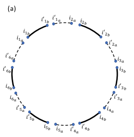
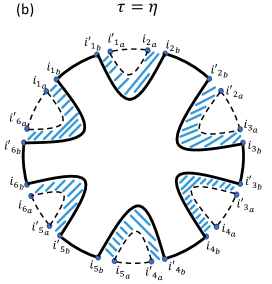
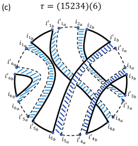
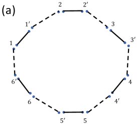
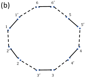
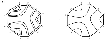
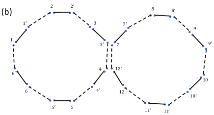
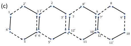
Figure 2: (a) shows the common exterior lines of all diagrams for different terms in (2.38), and (b) and (c) show examples of diagrams for two choices of τ𝜏\tau, for the case n=6𝑛6n=6.

Each term in the final expression in (2.38) can be given a diagrammatic representation, as shown in Fig. 2. We can insert the identity to write

ηAeA¯|α,τ=i1,i1,in,inηAeA¯|i1i¯1ini¯ni1i¯1ini¯n|α,τ,|im=|imaA|imbA¯,|i¯m=|i¯maA|i¯mbA¯.\begin{gathered}{\left\langle{\eta_{A}\otimes e_{\bar{A}}|{{\mathcal{I}}}_{\alpha},\tau}\right\rangle}=\sum_{i_{1},i^{\prime}_{1},...i_{n},i^{\prime}_{n}}\braket{\eta_{A}\otimes e_{\bar{A}}}{i_{1}\bar{i^{\prime}}_{1}...i_{n}\bar{i^{\prime}}_{n}}\braket{i_{1}\bar{i^{\prime}}_{1}...i_{n}\bar{i^{\prime}}_{n}}{{{\mathcal{I}}}_{{\alpha}},\tau},\\ \ket{i_{m}}=\ket{i_{m_{a}}}_{A}\ket{i_{m_{b}}}_{\bar{A}},\quad\ket{\bar{i^{\prime}}_{m}}=\ket{\bar{i^{\prime}}_{m_{a}}}_{A}\ket{\bar{i^{\prime}}_{m_{b}}}_{\bar{A}}\,.\end{gathered} (2.43)

The exterior of the diagram, which is the same for all τ𝜏\tau, represents ηAeA¯|i1i¯1ini¯ninner-producttensor-productsubscript𝜂𝐴subscript𝑒¯𝐴subscript𝑖1subscript¯superscript𝑖1subscript𝑖𝑛subscript¯superscript𝑖𝑛\braket{\eta_{A}\otimes e_{\bar{A}}}{i_{1}\bar{i^{\prime}}_{1}...i_{n}\bar{i^{\prime}}_{n}} by connecting imasubscript𝑖subscript𝑚𝑎i_{m_{a}} with iη(m)asubscriptsuperscript𝑖𝜂subscript𝑚𝑎i^{\prime}_{\eta(m)_{a}} using dashed lines, and imbsubscript𝑖subscript𝑚𝑏i_{m_{b}} with imbsubscriptsuperscript𝑖subscript𝑚𝑏i^{\prime}_{m_{b}} using solid lines, as shown in Fig. 2(a). The interior of the diagram represents i1i¯1ini¯n|α,τinner-productsubscript𝑖1subscript¯superscript𝑖1subscript𝑖𝑛subscript¯superscript𝑖𝑛subscript𝛼𝜏\braket{i_{1}\bar{i^{\prime}}_{1}...i_{n}\bar{i^{\prime}}_{n}}{{{\mathcal{I}}}_{{\alpha}},\tau}, by connecting imsubscript𝑖𝑚i_{m} with iτ(m)subscriptsuperscript𝑖𝜏𝑚i^{\prime}_{\tau(m)}, as shown for two examples in Fig. 2(b) and (c). Roughly, each solid loop in the resulting diagram gives a power of dA¯subscript𝑑¯𝐴d_{\bar{A}} and each dashed loop gives a power of dAsubscript𝑑𝐴d_{A}, where dAsubscript𝑑𝐴d_{A} and dA¯subscript𝑑¯𝐴d_{\bar{A}} are respectively the effective Hilbert space dimensions of A𝐴A and A¯¯𝐴\bar{A}.555When αsubscript𝛼{{\mathcal{I}}}_{\alpha} can be factorized between A𝐴A and A¯¯𝐴\bar{A}, i.e. α=AA¯subscript𝛼tensor-productsubscript𝐴subscript¯𝐴{{\mathcal{I}}}_{\alpha}={{\mathcal{I}}}_{A}\otimes{{\mathcal{I}}}_{\bar{A}}, we can define the effective dimensions as dA=TrAAsubscript𝑑𝐴subscriptTr𝐴subscript𝐴d_{A}=\text{Tr}_{A}{{\mathcal{I}}}_{A} and dA¯=TrA¯A¯subscript𝑑¯𝐴subscriptTr¯𝐴subscript¯𝐴d_{\bar{A}}=\text{Tr}_{\bar{A}}{{\mathcal{I}}}_{\bar{A}}. When αsubscript𝛼{{\mathcal{I}}}_{\alpha} cannot be factorized, they can be estimated by counting the numbers of degrees of freedom of the subsystems. The number of solid and dashed loops in a diagram is respectively equal to k(τ)𝑘𝜏k(\tau) (the number of cycles in permutation τ𝜏\tau) and k(η1τ)𝑘superscript𝜂1𝜏k(\eta^{-1}\tau). We therefore find

ηAeA¯|α,τdAk(η1τ)dA¯k(τ).similar-toinner-producttensor-productsubscript𝜂𝐴subscript𝑒¯𝐴subscript𝛼𝜏superscriptsubscript𝑑𝐴𝑘superscript𝜂1𝜏superscriptsubscript𝑑¯𝐴𝑘𝜏\braket{\eta_{A}\otimes e_{\bar{A}}}{{{\mathcal{I}}}_{{\alpha}},\tau}\sim d_{A}^{k(\eta^{-1}\tau)}d_{\bar{A}}^{k(\tau)}. (2.44)

For any permutation τ𝜏\tau, we have the inequality

k(τ)+k(η1τ)n+1,𝑘𝜏𝑘superscript𝜂1𝜏𝑛1k(\tau)+k(\eta^{-1}\tau)\leq n+1, (2.45)

and the permutations for which this inequality is saturated are the ones associated with planar diagrams such as Fig. 2(b).

From (2.44), when A𝐴A is much smaller than A¯¯𝐴\bar{A}, i.e. dAdA¯much-less-thansubscript𝑑𝐴subscript𝑑¯𝐴d_{A}\ll d_{\bar{A}}, the permutation τ=e𝜏𝑒\tau=e, which maximizes k(τ)𝑘𝜏k(\tau), dominates, and we have

𝒵n,A=𝒵n,A(eq),subscript𝒵𝑛𝐴superscriptsubscript𝒵𝑛𝐴eq\mathcal{Z}_{n,A}=\mathcal{Z}_{n,A}^{({\rm eq})}, (2.46)

where 𝒵n,A(eq)superscriptsubscript𝒵𝑛𝐴eq\mathcal{Z}_{n,A}^{({\rm eq})} is the Renyi partition function for A𝐴A in the state ρ(eq)superscript𝜌eq\rho^{(\rm eq)}. When A𝐴A is much larger than A¯¯𝐴\bar{A}, i.e. dAdA¯much-greater-thansubscript𝑑𝐴subscript𝑑¯𝐴d_{A}\gg d_{\bar{A}}, τ=η𝜏𝜂\tau=\eta, which maximizes k(η1τ)𝑘superscript𝜂1𝜏k(\eta^{-1}\tau), dominates

𝒵n,A=𝒵n,A¯(eq).subscript𝒵𝑛𝐴superscriptsubscript𝒵𝑛¯𝐴eq\mathcal{Z}_{n,A}=\mathcal{Z}_{n,\bar{A}}^{({\rm eq})}\ . (2.47)

Except for a crossover region around dAdA¯similar-tosubscript𝑑𝐴subscript𝑑¯𝐴d_{A}\sim d_{\bar{A}} where the behavior may be more complicated, we then have

Sn,A=min(Sn,A(eq),Sn,A¯(eq)),n2formulae-sequencesubscript𝑆𝑛𝐴minsuperscriptsubscript𝑆𝑛𝐴eqsuperscriptsubscript𝑆𝑛¯𝐴eq𝑛2S_{n,A}={\rm min}\left(S_{n,A}^{\rm(eq)},S_{n,\bar{A}}^{\rm(eq)}\right),\qquad n\geq 2 (2.48)

where Sn,A(eq)superscriptsubscript𝑆𝑛𝐴eqS_{n,A}^{(\rm eq)} denotes the n𝑛n-th Renyi entropy for subsystem A𝐴A in the equilibrium density operator ρ(eq)superscript𝜌eq\rho^{(\rm eq)}.

When SAsubscript𝑆𝐴S_{A} can be obtained from Sn,Asubscript𝑆𝑛𝐴S_{n,A} by analytic continuation to n=1𝑛1n=1, (2.48) implies

SA=min(SA(eq),SA¯(eq)),subscript𝑆𝐴minsuperscriptsubscript𝑆𝐴eqsuperscriptsubscript𝑆¯𝐴eqS_{A}={\rm min}(S_{A}^{\rm(eq)},S_{\bar{A}}^{\rm(eq)}),\, (2.49)

where SA(eq)superscriptsubscript𝑆𝐴eqS_{A}^{(\rm eq)} is the entanglement entropy for subsystem A𝐴A in ρ(eq)superscript𝜌eq\rho^{(\rm eq)}. In cases where the system AA¯𝐴¯𝐴A\bar{A} is inhomogeneous, in general (2.49) cannot be deduced by analytic continuation. We show in two such examples in Appendix F that (2.49) still holds, and will assume in the later discussion in this paper that it holds in general.

When αsubscript𝛼{{\mathcal{I}}}_{\alpha} can be factorized

αAA¯,subscript𝛼tensor-productsubscript𝐴subscript¯𝐴{{\mathcal{I}}}_{\alpha}\approx{{\mathcal{I}}}_{A}\otimes{{\mathcal{I}}}_{\bar{A}}, (2.50)

equations (2.38) can be written more explicitly in terms of partition functions of A𝐴A and A¯¯𝐴\bar{A}

Zm,A=TrAAm,Zm,A¯=TrA¯A¯m,formulae-sequencesubscript𝑍𝑚𝐴subscriptTr𝐴superscriptsubscript𝐴𝑚subscript𝑍𝑚¯𝐴subscriptTr¯𝐴superscriptsubscript¯𝐴𝑚Z_{m,A}={\rm Tr}_{A}{{\mathcal{I}}}_{A}^{m},\qquad Z_{m,\bar{A}}={\rm Tr}_{\bar{A}}{{\mathcal{I}}}_{\bar{A}}^{m},\quad (2.51)

as

𝒵n,Asubscript𝒵𝑛𝐴\displaystyle{\mathcal{Z}}_{n,A} 1Z1nτ(Zm1,AZml,A)(Zn1,A¯Znk,A¯),absent1superscriptsubscript𝑍1𝑛subscript𝜏subscript𝑍subscript𝑚1𝐴subscript𝑍subscript𝑚𝑙𝐴subscript𝑍subscript𝑛1¯𝐴subscript𝑍subscript𝑛𝑘¯𝐴\displaystyle\approx{1\over Z_{1}^{n}}\sum_{\tau}\left(Z_{m_{1},A}\cdots Z_{m_{l},A}\right)\left(Z_{n_{1},\bar{A}}\cdots Z_{n_{k},\bar{A}}\right)\ , (2.52)

where k𝑘k is the number of cycles of τ𝜏\tau with n1,nksubscript𝑛1subscript𝑛𝑘n_{1},\cdots n_{k} the lengths of the corresponding cycles, and l𝑙l is the number of cycles of τη1𝜏superscript𝜂1\tau\eta^{-1} with m1,mlsubscript𝑚1subscript𝑚𝑙m_{1},\cdots m_{l} the lengths of the corresponding cycles.

2.3.2 Mixed states

The equilibrium approximation can also be applied to a system A=A1A2𝐴subscript𝐴1subscript𝐴2A=A_{1}\cup A_{2} in a mixed state ρAsubscript𝜌𝐴\rho_{A} that is in macroscopic equilibrium, but is far from the thermal density operators [1].

Suppose the system starts with a far-from equilibrium mixed state ρ0,Asubscript𝜌0𝐴\rho_{0,A}, which evolves under unitary evolution operator UAsubscript𝑈𝐴U_{A} to ρA=UAρ0,AUAsubscript𝜌𝐴subscript𝑈𝐴subscript𝜌0𝐴subscriptsuperscript𝑈𝐴\rho_{A}=U_{A}\rho_{0,A}U^{\dagger}_{A}. All the moments of ρ0,Asubscript𝜌0𝐴\rho_{0,A} are also preserved by the time evolution

zn,A=Trρ0,An=TrρAn=Tr(UAρ0,AUA)n=η|(UAUA)n|ρ0,A,e,n=2,.formulae-sequencesubscript𝑧𝑛𝐴Trsuperscriptsubscript𝜌0𝐴𝑛Trsubscriptsuperscript𝜌𝑛𝐴Trsuperscriptsubscript𝑈𝐴subscript𝜌0𝐴superscriptsubscript𝑈𝐴𝑛quantum-operator-product𝜂superscripttensor-productsubscript𝑈𝐴subscriptsuperscript𝑈𝐴𝑛subscript𝜌0𝐴𝑒𝑛2z_{n,A}=\text{Tr}\rho_{0,A}^{n}=\text{Tr}\rho^{n}_{A}=\text{Tr}(U_{A}\rho_{0,A}U_{A}^{\dagger})^{n}={\left\langle{\eta|(U_{A}\otimes U^{{\dagger}}_{A})^{n}|\rho_{0,A},e}\right\rangle},\quad n=2,\cdots\ . (2.53)

The statement that ρ0,Asubscript𝜌0𝐴\rho_{0,A} is far-from-equilibrium is imposed by requiring that the nlimit-from𝑛n-th Renyi entropy of ρ0,Asubscript𝜌0𝐴\rho_{0,A} is smaller than the equilibrium entropy of A𝐴A. For example, this condition is satisfied if we have

zn,AZA(n1)f,0f<1.formulae-sequencesimilar-tosubscript𝑧𝑛𝐴superscriptsubscript𝑍𝐴𝑛1𝑓0𝑓1z_{n,A}\sim Z_{A}^{-(n-1)f}\,,\quad 0\leq f<1\,. (2.54)

Assuming that ρAsubscript𝜌𝐴\rho_{A} can be approximated by an equilibrium density operator ρA(eq)=1ZAAsubscriptsuperscript𝜌eq𝐴1subscript𝑍𝐴subscript𝐴\rho^{(\rm eq)}_{A}={1\over Z_{A}}{{\mathcal{I}}}_{A} and applying the equilibrium approximation by inserting the projector (2.35) in (2.53) and ignoring terms with στ𝜎𝜏\sigma\neq\tau, we have

zn,A1Z2,Anτη|A,τA,τ|ρ0,A,e,subscript𝑧𝑛𝐴1superscriptsubscript𝑍2𝐴𝑛subscript𝜏inner-product𝜂subscript𝐴𝜏inner-productsubscript𝐴𝜏subscript𝜌0𝐴𝑒z_{n,A}\approx{1\over Z_{2,A}^{n}}\sum_{\tau}{\left\langle{\eta|{{\mathcal{I}}}_{A},\tau}\right\rangle}{\left\langle{{{\mathcal{I}}}_{A},\tau|\rho_{0,A},e}\right\rangle}, (2.55)

which can be further simplified to the following constraints on Asubscript𝐴{{\mathcal{I}}}_{A} under the out-of-equilibrium assumption (2.54)

Tr(Aρ0,A)nzn,AZ2,AnZAn,Zn,A=TrAAn,ZA=Z1,A.formulae-sequenceTrsuperscriptsubscript𝐴subscript𝜌0𝐴𝑛subscript𝑧𝑛𝐴superscriptsubscript𝑍2𝐴𝑛superscriptsubscript𝑍𝐴𝑛formulae-sequencesubscript𝑍𝑛𝐴subscriptTr𝐴superscriptsubscript𝐴𝑛subscript𝑍𝐴subscript𝑍1𝐴\text{Tr}({{\mathcal{I}}}_{A}\rho_{0,A})^{n}\approx z_{n,A}{Z_{2,A}^{n}\over Z_{A}^{n}},\quad Z_{n,A}=\text{Tr}_{A}{{\mathcal{I}}}_{A}^{n},\quad Z_{A}=Z_{1,A}\ . (2.56)

The Renyi partition functions for A1subscript𝐴1A_{1} can then be approximated as

𝒵n,A1[𝒵n,A1]eqapprox=1ZAnτηA1eA2|A,τi=1k(τ)TrAρ0,Ani,n=2,3,formulae-sequencesubscript𝒵𝑛subscript𝐴1subscriptdelimited-[]subscript𝒵𝑛subscript𝐴1eqapprox1superscriptsubscript𝑍𝐴𝑛subscript𝜏inner-producttensor-productsubscript𝜂subscript𝐴1subscript𝑒subscript𝐴2subscript𝐴𝜏superscriptsubscriptproduct𝑖1𝑘𝜏subscriptTr𝐴superscriptsubscript𝜌0𝐴subscript𝑛𝑖𝑛23{\mathcal{Z}}_{n,A_{1}}\approx[{\mathcal{Z}}_{n,A_{1}}]_{\rm eq\,approx}={1\over Z_{A}^{n}}\sum_{\tau}{\left\langle{\eta_{A_{1}}\otimes e_{A_{2}}|{{\mathcal{I}}}_{A},\tau}\right\rangle}\prod_{i=1}^{k(\tau)}\text{Tr}_{A}\rho_{0,A}^{n_{i}},\quad n=2,3,\cdots (2.57)

where k(τ)𝑘𝜏k(\tau) is the number of cycles of τ𝜏\tau with n1,nk(τ)subscript𝑛1subscript𝑛𝑘𝜏n_{1},\cdots n_{k(\tau)} the lengths of the cycles.

The above discussion can be further generalized by embedding A𝐴A in a larger system S=AB𝑆𝐴𝐵S=A\cup B, with the total system S𝑆S in an initial pure state |Ψ0ketsubscriptΨ0\ket{\Psi_{0}} evolved to |Ψ=U|Ψ0ketΨ𝑈ketsubscriptΨ0\ket{\Psi}=U\ket{\Psi_{0}} in macroscopic equilibrium666A𝐴A and B𝐵B in principle do not have to be in equilibrium with each other.. Suppose |ΨketΨ\ket{\Psi} can be approximated macroscopically by ρ(eq)=1Z1superscript𝜌eq1subscript𝑍1\rho^{(\rm eq)}={1\over Z_{1}}{{\mathcal{I}}}. We then have

𝒵n,A11Z1nτηA1eA2B|,τ.subscript𝒵𝑛subscript𝐴11superscriptsubscript𝑍1𝑛subscript𝜏inner-producttensor-productsubscript𝜂subscript𝐴1subscript𝑒subscript𝐴2𝐵𝜏{\mathcal{Z}}_{n,A_{1}}\approx{1\over Z_{1}^{n}}\sum_{\tau}{\left\langle{\eta_{A_{1}}\otimes e_{A_{2}B}|{{\mathcal{I}}},\tau}\right\rangle}\ . (2.58)

This generalizes (2.57) as under the evolution of U𝑈U for the full system S𝑆S, the evolution from the initial density operator ρ0,Asubscript𝜌0𝐴\rho_{0,A} to ρAsubscript𝜌𝐴\rho_{A} is in general not unitary. To recover (2.57) we take U=UAUB𝑈tensor-productsubscript𝑈𝐴subscript𝑈𝐵U=U_{A}\otimes U_{B} to be factorized between A𝐴A and B𝐵B, in which case the equilibrium density operator =ABtensor-productsubscript𝐴subscript𝐵{{\mathcal{I}}}={{\mathcal{I}}}_{A}\otimes{{\mathcal{I}}}_{B} should also factorize, and (2.58) can be written as

𝒵n,A1=1ZAnτηA1eA2|A,τi=1k(τ)Z^ni,B,Z^n,B:=1ZBnTrBBn.formulae-sequencesubscript𝒵𝑛subscript𝐴11superscriptsubscript𝑍𝐴𝑛subscript𝜏inner-producttensor-productsubscript𝜂subscript𝐴1subscript𝑒subscript𝐴2subscript𝐴𝜏superscriptsubscriptproduct𝑖1𝑘𝜏subscript^𝑍subscript𝑛𝑖𝐵assignsubscript^𝑍𝑛𝐵1superscriptsubscript𝑍𝐵𝑛subscriptTr𝐵superscriptsubscript𝐵𝑛{\mathcal{Z}}_{n,A_{1}}={1\over Z_{A}^{n}}\sum_{\tau}{\left\langle{\eta_{A_{1}}\otimes e_{A_{2}}|{{\mathcal{I}}}_{A},\tau}\right\rangle}\prod_{i=1}^{k(\tau)}\hat{Z}_{n_{i},B},\quad\hat{Z}_{n,B}:={1\over Z_{B}^{n}}{\rm\text{Tr}}_{B}{{\mathcal{I}}}_{B}^{n}\ . (2.59)

Equations (2.57) and (2.59) are equal provided that we choose the initial state ρ0,Bsubscript𝜌0𝐵\rho_{0,B} such that

TrBρ0,Bm=1ZBmTrBBm.subscriptTr𝐵superscriptsubscript𝜌0𝐵𝑚1superscriptsubscript𝑍𝐵𝑚subscriptTr𝐵superscriptsubscript𝐵𝑚{\rm Tr}_{B}\rho_{0,B}^{m}={1\over Z_{B}^{m}}{\rm Tr}_{B}{{\mathcal{I}}}_{B}^{m}\,. (2.60)

Then since the initial state is pure, zn,Asubscript𝑧𝑛𝐴z_{n,A} is also given by (2.60). The requirement that ρ0,Asubscript𝜌0𝐴\rho_{0,A} is out-of-equilibrium is then equivalent to the requirement that ZBZAmuch-greater-thansubscript𝑍𝐵subscript𝑍𝐴Z_{B}\gg Z_{A}.

The relation between (2.58) and (2.57) also gives a way to estimate which permutation dominates in (2.57). From (2.58), when A1subscript𝐴1A_{1} is smaller (larger) than A2Bsubscript𝐴2𝐵A_{2}B, the dominant contribution is τ=e𝜏𝑒\tau=e (τ=η𝜏𝜂\tau=\eta). Translating these statements to the notation of (2.57), we conclude that

Sn,A1={Sn,A1(eq)Sn,A1(eq)<Sn,A2(eq)+Sn,ASn,A2(eq)+Sn,ASn,A1(eq)>Sn,A2(eq)+Sn,A.subscript𝑆𝑛subscript𝐴1casessuperscriptsubscript𝑆𝑛subscript𝐴1eqsuperscriptsubscript𝑆𝑛subscript𝐴1eqsuperscriptsubscript𝑆𝑛subscript𝐴2eqsubscript𝑆𝑛𝐴superscriptsubscript𝑆𝑛subscript𝐴2eqsubscript𝑆𝑛𝐴superscriptsubscript𝑆𝑛subscript𝐴1eqsuperscriptsubscript𝑆𝑛subscript𝐴2eqsubscript𝑆𝑛𝐴S_{n,A_{1}}=\begin{cases}S_{n,A_{1}}^{({\rm eq})}&S_{n,A_{1}}^{(\rm eq)}<S_{n,A_{2}}^{(\rm eq)}+S_{n,A}\cr S_{n,A_{2}}^{({\rm eq})}+S_{n,A}&S_{n,A_{1}}^{(\rm eq)}>S_{n,A_{2}}^{(\rm eq)}+S_{n,A}\end{cases}\ . (2.61)

In applying (2.58) to explicit calculations, we will need to make assumptions regarding B𝐵B in the equilibrium density operator ρ(eq)superscript𝜌eq\rho^{(\rm eq)} for the full system, which may be considered as specifying different universality classes for ρAsubscript𝜌𝐴\rho_{A}.

2.4 The Petz recovery map

An important question concerning a quantum channel 𝒩𝒩{{\mathcal{N}}} is whether or not it is reversible i.e. whether there exists a recovery channel 𝒩𝒩{{\mathcal{N}}} such that for any state ρ𝜌\rho, 𝒩(ρ)=ρ𝒩𝜌𝜌{\mathcal{R}}\circ{{\mathcal{N}}}(\rho)=\rho. This question plays a central role, for example, in the theory of quantum error correction as well as quantum thermalization. If the quantum channel is unitary, the initial state is perfectly recovered by acting on the output with the adjoint of the unitary. In the other extreme, a quantum channel could replace all states with the maximally mixed state, in which case an initial state is unrecoverable as the information about it is completely lost. A recovery map that is independent of the initial state ρ𝜌\rho is called universal.

It follows from a theorem by Petz [36, 37, 38] that a quantum channel 𝒩𝒩{{\mathcal{N}}} is reversible if and only if the data processing inequality is saturated

D(ρ||σ)=D(𝒩(ρ)||𝒩(σ))𝐷𝜌𝜎𝐷𝒩𝜌𝒩𝜎\displaystyle D(\rho\lvert\rvert\sigma)=D(\mathcal{N}(\rho)\lvert\rvert\mathcal{N}(\sigma)) (2.62)

for all ρ,σ𝜌𝜎\rho,\sigma. Here, D(ρ||σ)𝐷𝜌𝜎D(\rho\lvert\rvert\sigma) is the relative entropy. Furthermore, suppose we fix some reference state σ𝜎\sigma. Then, for any state X𝑋X in the support of 𝒩(σ)𝒩𝜎{{\mathcal{N}}}(\sigma), there exists a recovery channel {\mathcal{R}}. This channel is given explicitly by the Petz map,

𝒫σ,𝒩(X)=σ12𝒩((𝒩(σ))12X(𝒩(σ))12)σ12,subscript𝒫𝜎𝒩𝑋superscript𝜎12superscript𝒩superscript𝒩𝜎12𝑋superscript𝒩𝜎12superscript𝜎12\displaystyle\mathcal{P}_{\sigma,\mathcal{N}}(X)=\sigma^{\frac{1}{2}}\mathcal{N}^{\dagger}\left((\mathcal{N}(\sigma))^{-\frac{1}{2}}X(\mathcal{N}(\sigma))^{-\frac{1}{2}}\right)\sigma^{\frac{1}{2}}, (2.63)

where 𝒩superscript𝒩\mathcal{N}^{\dagger} is the adjoint map of 𝒩𝒩{{\mathcal{N}}}. As a basic check, relative entropy is invariant under unitary channels ρUρU𝜌𝑈𝜌superscript𝑈\rho\to U\rho U^{\dagger}, and we find from (2.63), 𝒫σ,𝒩(X)=UXUsubscript𝒫𝜎𝒩𝑋superscript𝑈𝑋𝑈\mathcal{P}_{\sigma,\mathcal{N}}(X)=U^{\dagger}XU.

Interestingly, it has recently been understood that the change of relative entropy under quantum channels places strict bounds on how well a state can be recovered. The basic idea is intuitive; if two states that were initially easily distinguishable become nearly indistinguishable under a channel, then it should be impossible to identify what the initial states were using only information about the indistinguishable output states. In particular, it can be shown [39] that there exists a recovery map σ,𝒩subscript𝜎𝒩{\mathcal{R}}_{\sigma,{{\mathcal{N}}}} with σ,𝒩𝒩(σ)=σsubscript𝜎𝒩𝒩𝜎𝜎\mathcal{R}_{\sigma,\mathcal{N}}\circ\mathcal{N}(\sigma)=\sigma satisfying777This was proven for Type I von Neumann algebras but was recently generalized to the Type III algebras relevant to quantum field theory that we will model [40]. This technicality will not play an important role for us.,

F(ρ,[σ,𝒩𝒩](ρ))exp(D(𝒩(ρ)||𝒩(σ))D(ρ||σ)),\displaystyle F(\rho,[\mathcal{R}_{\sigma,\mathcal{N}}\circ\mathcal{N}](\rho))\geq\exp(D(\mathcal{N}(\rho)||\mathcal{N}(\sigma))-D(\rho||\sigma)), (2.64)

where F𝐹F is the fidelity, defined as

F(ρ,σ):=(Tr[ρσρ])2.assign𝐹𝜌𝜎superscriptTrdelimited-[]𝜌𝜎𝜌2\displaystyle F(\rho,\sigma):=\left(\text{Tr}\left[\sqrt{\sqrt{\rho}\sigma\sqrt{\rho}}\right]\right)^{2}\ . (2.65)

For example, the bound (2.64) holds for an explicit but complicated recovery channel called the twirled Petz map [39].

For the quantum channel that we are interested in this paper, consider a system DB=RB𝐷𝐵𝑅superscript𝐵D\cup B=R\cup B^{\prime} in the initial state ρDρBtensor-productsubscript𝜌𝐷subscript𝜌𝐵\rho_{D}\otimes\rho_{B}, evolve it for a while, and then trace out a portion Bsuperscript𝐵B^{\prime} of the full system. If we take ρBsubscript𝜌𝐵\rho_{B} to be some fixed state, this gives a quantum channel from D𝐷D to R𝑅R,

𝒩(ρD)=TrB[U(ρDρB)U].𝒩subscript𝜌𝐷subscriptTrsuperscript𝐵delimited-[]𝑈tensor-productsubscript𝜌𝐷subscript𝜌𝐵superscript𝑈\displaystyle\mathcal{N}(\rho_{D})=\text{Tr}_{B^{\prime}}\left[U\left(\rho_{D}\otimes\rho_{B}\right)U^{\dagger}\right]\ . (2.66)

The corresponding 𝒩superscript𝒩{{\mathcal{N}}}^{\dagger} from R𝑅R to D𝐷D is then given by

𝒩(ϕR)=TrB(ρBU(ϕR𝟙B)U).superscript𝒩subscriptitalic-ϕ𝑅subscriptTr𝐵subscript𝜌𝐵superscript𝑈tensor-productsubscriptitalic-ϕ𝑅subscript1superscript𝐵𝑈\displaystyle\mathcal{N}^{\dagger}(\phi_{R})=\text{Tr}_{B}\left(\rho_{B}U^{\dagger}\left(\phi_{R}\otimes\mathbbm{1}_{B^{\prime}}\right)U\right)\ . (2.67)

Applying (2.63) to this case and imposing a replica trick, we have

𝒫σD,𝒩𝒩(ρD)=limm12σD12TrB[ρBU(𝒩(σD)m𝒩(ρD)𝒩(σD)m𝟙B)U]σD12.subscript𝒫subscript𝜎𝐷𝒩𝒩subscript𝜌𝐷subscript𝑚12superscriptsubscript𝜎𝐷12subscriptTr𝐵delimited-[]subscript𝜌𝐵superscript𝑈tensor-product𝒩superscriptsubscript𝜎𝐷𝑚𝒩subscript𝜌𝐷𝒩superscriptsubscript𝜎𝐷𝑚subscript1superscript𝐵𝑈superscriptsubscript𝜎𝐷12\displaystyle\mathcal{P}_{\sigma_{D},\mathcal{N}}\circ\mathcal{N}(\rho_{D})=\lim_{m\to-{{\frac{1}{2}}}}\sigma_{D}^{{\frac{1}{2}}}\text{Tr}_{B}\left[\rho_{B}U^{\dagger}\left({{\mathcal{N}}}(\sigma_{D})^{m}\mathcal{N}(\rho_{D}){{\mathcal{N}}}(\sigma_{D})^{m}\otimes\mathbbm{1}_{B^{\prime}}\right)U\right]\sigma_{D}^{{\frac{1}{2}}}\ . (2.68)

In some of our discussion below, an alternative analytic continuation will also be useful:

𝒫σD,𝒩𝒩(ρD)=limn112,n212σD12TrB[ρBU(𝒩(σD)n1𝒩(ρD)𝒩(σD)n2𝟙B)U]σD12.subscript𝒫subscript𝜎𝐷𝒩𝒩subscript𝜌𝐷subscriptsubscript𝑛112subscript𝑛212superscriptsubscript𝜎𝐷12subscriptTr𝐵delimited-[]subscript𝜌𝐵superscript𝑈tensor-product𝒩superscriptsubscript𝜎𝐷subscript𝑛1𝒩subscript𝜌𝐷𝒩superscriptsubscript𝜎𝐷subscript𝑛2subscript1superscript𝐵𝑈superscriptsubscript𝜎𝐷12\displaystyle\mathcal{P}_{\sigma_{D},\mathcal{N}}\circ\mathcal{N}(\rho_{D})=\lim_{\begin{subarray}{c}n_{1}\to-{{\frac{1}{2}}},\\ \,n_{2}\to-{{\frac{1}{2}}}\end{subarray}}\sigma_{D}^{{\frac{1}{2}}}\text{Tr}_{B}\left[\rho_{B}U^{\dagger}\left({{\mathcal{N}}}(\sigma_{D})^{n_{1}}\mathcal{N}(\rho_{D}){{\mathcal{N}}}(\sigma_{D})^{n_{2}}\otimes\mathbbm{1}_{B^{\prime}}\right)U\right]\sigma_{D}^{{\frac{1}{2}}}\ . (2.69)

When we take Bsuperscript𝐵B^{\prime} to be empty, then 𝒩𝒩{{\mathcal{N}}} is unitary, and 𝒩superscript𝒩{{\mathcal{N}}}^{\dagger} is the inverse evolution, for which the above equation gives ρDsubscript𝜌𝐷\rho_{D}. In the opposite limit, with Bsuperscript𝐵B^{\prime} being the full system, we have 𝒫σD,𝒩𝒩(ρD)=σDsubscript𝒫subscript𝜎𝐷𝒩𝒩subscript𝜌𝐷subscript𝜎𝐷\mathcal{P}_{\sigma_{D},\mathcal{N}}\circ\mathcal{N}(\rho_{D})=\sigma_{D} for any ρDsubscript𝜌𝐷\rho_{D}.

In the case where ρDsubscript𝜌𝐷\rho_{D} is a pure state, the fidelity of the Petz map can be written as an overlap

F(ρD,𝒫σD,𝒩𝒩(ρD))=TrD(ρD𝒫σD,𝒩𝒩(ρD))𝐹subscript𝜌𝐷subscript𝒫subscript𝜎𝐷𝒩𝒩subscript𝜌𝐷subscriptTr𝐷subscript𝜌𝐷subscript𝒫subscript𝜎𝐷𝒩𝒩subscript𝜌𝐷\displaystyle F(\rho_{D},\mathcal{P}_{\sigma_{D},\mathcal{N}}\circ\mathcal{N}(\rho_{D}))=\text{Tr}_{D}\left(\rho_{D}\mathcal{P}_{\sigma_{D},\mathcal{N}}\circ\mathcal{N}(\rho_{D})\right) (2.70)
=limm12Tr[U(σD12ρDσD12ρB)U𝒩(σD)m𝒩(ρD)𝒩(σD)m].absentsubscript𝑚12Trdelimited-[]𝑈tensor-productsuperscriptsubscript𝜎𝐷12subscript𝜌𝐷superscriptsubscript𝜎𝐷12subscript𝜌𝐵superscript𝑈𝒩superscriptsubscript𝜎𝐷𝑚𝒩subscript𝜌𝐷𝒩superscriptsubscript𝜎𝐷𝑚\displaystyle=\lim_{m\to-{{\frac{1}{2}}}}\text{Tr}\left[U\left(\sigma_{D}^{{\frac{1}{2}}}\rho_{D}\sigma_{D}^{{\frac{1}{2}}}\otimes\rho_{B}\right)U^{\dagger}{{\mathcal{N}}}(\sigma_{D})^{m}\mathcal{N}(\rho_{D}){{\mathcal{N}}}(\sigma_{D})^{m}\right]\ . (2.71)

or a similar overlap using (2.69). (2.68), (2.69), and (2.70) can all be evaluated by using the equilibrium approximation. If the Petz map works perfectly, without error, the fidelity will be one. At worst, the Petz map should output a random answer in which case the fidelity would be exponentially small in the entropy.

3 Equilibrium approximation for quantum-informational quantities

In addition to the Renyi and entanglement entropies, the equilibrium approximation can in principle be used to calculate any quantum informational quantities which can be defined using replicas. In this section, we consider a few quantities that will be used in the later discussion of the paper: Renyi and logarithmic negativities, relative entropy, reflected entropy, and the Petz recovery map.

3.1 Renyi and logarithmic negativities

We now describe the calculation of Renyi negativities between A1subscript𝐴1A_{1} and A2subscript𝐴2A_{2} by adding an auxiliary system B𝐵B to A𝐴A, and applying the equilibrium approximation to an equilibrated pure state |ΨketΨ\ket{\Psi} describing the full system S=AB𝑆𝐴𝐵S=A\cup B. There is also an alternative way to to calculate the negativities between A1subscript𝐴1A_{1} and A2subscript𝐴2A_{2} by directly applying the equilibrium approximation to the mixed state ρAsubscript𝜌𝐴\rho_{A}, analogous to the discussion for the Renyi entropies in Section 2.3.2.

Suppose the system is partitioned to AB𝐴𝐵A\cup B with =ABtensor-productsubscript𝐴subscript𝐵{{\mathcal{H}}}={{\mathcal{H}}}_{A}\otimes{{\mathcal{H}}}_{B} and the subsystem A𝐴A is in turn partitioned to A=A1A2𝐴subscript𝐴1subscript𝐴2A=A_{1}\cup A_{2} with A=12subscript𝐴tensor-productsubscript1subscript2{{\mathcal{H}}}_{A}={{\mathcal{H}}}_{1}\otimes{{\mathcal{H}}}_{2}. We are interested in

𝒵n(PT):=Tr(ρAT2)n=TrA(TrB(Uρ0U)T2)nassignsuperscriptsubscript𝒵𝑛PTTrsuperscriptsuperscriptsubscript𝜌𝐴subscript𝑇2𝑛subscriptTr𝐴superscriptsubscriptTr𝐵superscript𝑈subscript𝜌0superscript𝑈subscript𝑇2𝑛\displaystyle\mathcal{Z}_{n}^{(\rm PT)}:=\text{Tr}\left(\rho_{A}^{T_{2}}\right)^{n}=\text{Tr}_{A}\left(\text{Tr}_{B}\left(U\rho_{0}U^{\dagger}\right)^{T_{2}}\right)^{n} (3.1)

and the corresponding logarithmic negativity (A1,A2)=limn12log𝒵2n(PT)subscript𝐴1subscript𝐴2subscript𝑛12superscriptsubscript𝒵2𝑛PT\mathcal{E}(A_{1},A_{2})=\lim_{n\to{{\frac{1}{2}}}}\log\mathcal{Z}_{2n}^{(\rm PT)}.

Using the replica space ()nsuperscripttensor-product𝑛({{\mathcal{H}}}\otimes{{\mathcal{H}}})^{n} we can write (3.1) as

𝒵n(PT)=ηA1ηA21eB|(UU)n|ρ0,e,superscriptsubscript𝒵𝑛PTbratensor-productsubscript𝜂subscript𝐴1subscriptsuperscript𝜂1subscript𝐴2subscript𝑒𝐵superscripttensor-product𝑈superscript𝑈𝑛ketsubscript𝜌0𝑒\displaystyle\mathcal{Z}_{n}^{(\rm PT)}=\bra{\eta_{A_{1}}\otimes\eta^{-1}_{A_{2}}\otimes e_{B}}\left(U\otimes U^{\dagger}\right)^{n}\ket{\rho_{0},e}, (3.2)

where η=(n,n1,1)𝜂𝑛𝑛11\eta=(n,n-1,\cdots 1) is the cyclic permutation and its inverse η1superscript𝜂1\eta^{-1} is the anti-cyclic permutation.

We can insert the identity (2.34) twice in (3.2) to arrive at

𝒵n(PT)=ηA1ηA21eB|Pα|ρ0,e+ηA1ηA21eB|Q(UU)nQ|ρ0,e.superscriptsubscript𝒵𝑛PTbratensor-productsubscript𝜂subscript𝐴1subscriptsuperscript𝜂1subscript𝐴2subscript𝑒𝐵subscript𝑃𝛼ketsubscript𝜌0𝑒bratensor-productsubscript𝜂subscript𝐴1subscriptsuperscript𝜂1subscript𝐴2subscript𝑒𝐵𝑄superscripttensor-product𝑈superscript𝑈𝑛𝑄ketsubscript𝜌0𝑒\displaystyle\mathcal{Z}_{n}^{\rm(PT)}=\bra{\eta_{A_{1}}\otimes\eta^{-1}_{A_{2}}\otimes e_{B}}P_{\alpha}\ket{\rho_{0},e}+\bra{\eta_{A_{1}}\otimes\eta^{-1}_{A_{2}}\otimes e_{B}}Q\left(U\otimes U^{\dagger}\right)^{n}Q\ket{\rho_{0},e}\ . (3.3)

In the equilibrium approximation, we drop the second term in the above equation, which leads to a time-independent expression,

𝒵n(PT)superscriptsubscript𝒵𝑛PT\displaystyle\mathcal{Z}_{n}^{(\rm PT)} [𝒵n(PT)]eq approx:=1Z2nσ,τgτσηA1ηA21eB|α,τα,σ|ρ0,e\displaystyle\approx[\mathcal{Z}_{n}^{(\rm PT)}]_{\text{eq approx}}:=\frac{1}{Z_{2}^{n}}\sum_{\sigma,\tau}g^{\tau\sigma}\bra{\eta_{A_{1}}\otimes\eta^{-1}_{A_{2}}\otimes e_{B}}\mathcal{I}_{\alpha},\tau\rangle\bra{\mathcal{I}_{\alpha},\sigma}\rho_{0},e\rangle
=1Z1nσ,τgτσηA1ηA21eB|α,τ\displaystyle=\frac{1}{Z_{1}^{n}}\sum_{\sigma,\tau}g^{\tau\sigma}\bra{\eta_{A_{1}}\otimes\eta^{-1}_{A_{2}}\otimes e_{B}}\mathcal{I}_{\alpha},\tau\rangle
1Z1nτηA1ηA21eB|α,τ.\displaystyle\approx\frac{1}{Z_{1}^{n}}\sum_{\tau}\bra{\eta_{A_{1}}\otimes\eta^{-1}_{A_{2}}\otimes e_{B}}\mathcal{I}_{\alpha},\tau\rangle\ . (3.4)

In the second line above we used (2.39) and in the third line, we again used the fact that in the large Z1subscript𝑍1Z_{1} limit gστsubscript𝑔𝜎𝜏g_{\sigma\tau} can be approximated by the identity matrix. This final expression is independent of the initial state and only depends on the equilibrium density operator.

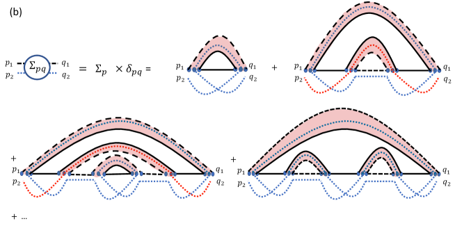
Each term in the final expression in (3.4) can be given a diagrammatic representation, as shown in Fig. 3. We can insert the identity to write

ηA1ηA21eB|α,τ=i1,i1,in,inηA1ηA21eB|i1i¯1ini¯ni1i¯1ini¯n|α,τ,|im=|imaA1|ima¯A2|imbB,|i¯m=|i¯maA1|i¯ma¯A2|i¯mbB.\begin{gathered}{\left\langle{\eta_{A_{1}}\otimes\eta^{-1}_{A_{2}}\otimes e_{B}|{{\mathcal{I}}}_{\alpha},\tau}\right\rangle}=\sum_{i_{1},i^{\prime}_{1},...i_{n},i^{\prime}_{n}}\braket{\eta_{A_{1}}\otimes\eta^{-1}_{A_{2}}\otimes e_{B}}{i_{1}\bar{i^{\prime}}_{1}...i_{n}\bar{i^{\prime}}_{n}}\braket{i_{1}\bar{i^{\prime}}_{1}...i_{n}\bar{i^{\prime}}_{n}}{{{\mathcal{I}}}_{{\alpha}},\tau}\,,\\ \ket{i_{m}}=\ket{i_{m_{a}}}_{A_{1}}\ket{i_{m_{\bar{a}}}}_{A_{2}}\ket{i_{m_{b}}}_{B},\quad\ket{\bar{i^{\prime}}_{m}}=\ket{\bar{i^{\prime}}_{m_{a}}}_{A_{1}}\ket{\bar{i^{\prime}}_{m_{\bar{a}}}}_{A_{2}}\ket{\bar{i^{\prime}}_{m_{b}}}_{B}\,.\end{gathered} (3.5)

The lower half of each diagram represents ηA1ηA21eB|i1i¯1ini¯ninner-producttensor-productsubscript𝜂subscript𝐴1subscriptsuperscript𝜂1subscript𝐴2subscript𝑒𝐵subscript𝑖1subscript¯superscript𝑖1subscript𝑖𝑛subscript¯superscript𝑖𝑛\braket{\eta_{A_{1}}\otimes\eta^{-1}_{A_{2}}\otimes e_{B}}{i_{1}\bar{i^{\prime}}_{1}...i_{n}\bar{i^{\prime}}_{n}} by connecting imasubscript𝑖subscript𝑚𝑎i_{m_{a}} with iη(m)asubscriptsuperscript𝑖𝜂subscript𝑚𝑎i^{\prime}_{\eta(m)_{a}} using dashed lines, ima¯subscript𝑖subscript𝑚¯𝑎i_{m_{\bar{a}}} with iη1(m)a¯subscriptsuperscript𝑖superscript𝜂1subscript𝑚¯𝑎i^{\prime}_{\eta^{-1}(m)_{\bar{a}}} using dotted lines, and imbsubscript𝑖subscript𝑚𝑏i_{m_{b}} with imbsubscriptsuperscript𝑖subscript𝑚𝑏i^{\prime}_{m_{b}} using solid lines, as shown in Fig. 3(a). The upper half of the diagram represents i1i¯1ini¯n|α,τinner-productsubscript𝑖1subscript¯superscript𝑖1subscript𝑖𝑛subscript¯superscript𝑖𝑛subscript𝛼𝜏\braket{i_{1}\bar{i^{\prime}}_{1}...i_{n}\bar{i^{\prime}}_{n}}{{{\mathcal{I}}}_{{\alpha}},\tau}, by connecting imsubscript𝑖𝑚i_{m} with iτ(m)subscriptsuperscript𝑖𝜏𝑚i^{\prime}_{\tau(m)}, as shown for two examples in Fig. 3(b) and (c). In the resulting diagram, roughly each solid loop gives a power of dBsubscript𝑑𝐵d_{B}, each dashed loop gives a power of dA1subscript𝑑subscript𝐴1d_{A_{1}}, and each dotted loop gives a power of dA2subscript𝑑subscript𝐴2d_{A_{2}}, where dPsubscript𝑑𝑃d_{P} is the effective Hilbert space dimension of subsystem P𝑃P. The number of solid, dashed, and dotted loops in a diagram is respectively equal to k(τ)𝑘𝜏k(\tau), k(η1τ)𝑘superscript𝜂1𝜏k(\eta^{-1}\tau), and k(ητ)𝑘𝜂𝜏k(\eta\tau). We therefore find

ηA1ηA21eB|α,τdA1k(η1τ)dA2k(ητ)dBk(τ).similar-toinner-producttensor-productsubscript𝜂subscript𝐴1subscriptsuperscript𝜂1subscript𝐴2subscript𝑒𝐵subscript𝛼𝜏superscriptsubscript𝑑subscript𝐴1𝑘superscript𝜂1𝜏superscriptsubscript𝑑subscript𝐴2𝑘𝜂𝜏superscriptsubscript𝑑𝐵𝑘𝜏\braket{\eta_{A_{1}}\otimes\eta^{-1}_{A_{2}}\otimes e_{B}}{{{\mathcal{I}}}_{{\alpha}},\tau}\sim d_{A_{1}}^{k(\eta^{-1}\tau)}d_{A_{2}}^{k(\eta\tau)}d_{B}^{k(\tau)}. (3.6)
Refer to caption
Refer to caption
Refer to caption
Figure 3: (a) shows the common lines of all diagrams for different terms in (3.4), and (b) and (c) show examples for two choices of τ𝜏\tau, for the case n=4𝑛4n=4. The dotted loops are shown in two different colors in (c) to make the distinction between different loops clear.

The sum of these powers satisfies the inequality

k(η1τ)+k(ητ)+k(τ){3n/2+2n even(3n+3)/2n odd.𝑘superscript𝜂1𝜏𝑘𝜂𝜏𝑘𝜏cases3𝑛22𝑛 even3𝑛32𝑛 oddk(\eta^{-1}\tau)+k(\eta\tau)+k(\tau)\leq\begin{cases}3n/2+2&n\text{ even}\\ (3n+3)/2&n\text{ odd}\end{cases}\ . (3.7)

The permutations for which this inequality is saturated are described in Appendix A.

We note

ηA1ηA21eB|α,τ=(μ1η)A1(μ2η1)A2(μ3)B|α,(μ1τ)A1(μ2τ)A2(μ3τ)B\bra{\eta_{A_{1}}\otimes\eta^{-1}_{A_{2}}\otimes e_{B}}\mathcal{I}_{\alpha},\tau\rangle=\bra{(\mu_{1}\eta)_{A_{1}}(\mu_{2}\eta^{-1})_{A_{2}}(\mu_{3})_{B}}\mathcal{I}_{\alpha},(\mu_{1}\tau)_{A_{1}}(\mu_{2}\tau)_{A_{2}}(\mu_{3}\tau)_{B}\rangle (3.8)

for arbitrary μ1,2,3𝒮nsubscript𝜇123subscript𝒮𝑛\mu_{1,2,3}\in{\mathcal{S}}_{n}, and

ηA1ηA21eB|α,τ=(ημ)A1(η1μ)A2μB|α,(τμ)A1(τμ)A2(τμ)B,μ𝒮n.\bra{\eta_{A_{1}}\otimes\eta^{-1}_{A_{2}}\otimes e_{B}}\mathcal{I}_{\alpha},\tau\rangle={\left\langle{(\eta\mu)_{A_{1}}(\eta^{-1}\mu)_{A_{2}}\mu_{B}|{{\mathcal{I}}}_{\alpha},(\tau\mu)_{A_{1}}(\tau\mu)_{A_{2}}(\tau\mu)_{B}}\right\rangle},\quad\mu\in{\mathcal{S}}_{n}\ . (3.9)

The expression (3.4) passes various consistency checks. Firstly, we have

𝒵n(PT)(A1,A2)=𝒵n(PT)(A2,A1),superscriptsubscript𝒵𝑛PTsubscript𝐴1subscript𝐴2superscriptsubscript𝒵𝑛PTsubscript𝐴2subscript𝐴1\mathcal{Z}_{n}^{(\rm PT)}(A_{1},A_{2})=\mathcal{Z}_{n}^{(\rm PT)}(A_{2},A_{1}), (3.10)

which can be shown as follows. Since η𝜂\eta and η1superscript𝜂1\eta^{-1} have the same cycle structure, there exists some element σSn𝜎subscript𝑆𝑛\sigma\in S_{n} such that η1=σησ1superscript𝜂1𝜎𝜂superscript𝜎1\eta^{-1}=\sigma\eta\sigma^{-1} and η=ση1σ1𝜂𝜎superscript𝜂1superscript𝜎1\eta=\sigma\eta^{-1}\sigma^{-1}. We then have from (3.8)–(3.9)

ηA1ηA21eB|α,τ=ηA11ηA2eB|α,σ1τσ\bra{\eta_{A_{1}}\otimes\eta^{-1}_{A_{2}}\otimes e_{B}}\mathcal{I}_{\alpha},\tau\rangle=\bra{\eta^{-1}_{A_{1}}\otimes\eta_{A_{2}}\otimes e_{B}}\mathcal{I}_{\alpha},\sigma^{-1}\tau\sigma\rangle (3.11)

and thus (3.10) results upon summing over τ𝜏\tau.

Next, consider n=2𝑛2n=2, where 𝒵2(PT)superscriptsubscript𝒵2PT\mathcal{Z}_{2}^{(\rm PT)} should give the same answer as 𝒵2(A)subscriptsuperscript𝒵𝐴2\mathcal{Z}^{(A)}_{2}, the second moment of the density matrix that has not been partially transposed. For n=2𝑛2n=2, η=η1𝜂superscript𝜂1\eta=\eta^{-1} because both are swap operators, so this check immediately passes.

Finally, consider the case where B𝐵B is not present, i.e. ρAsubscript𝜌𝐴\rho_{A} is a pure state

𝒵n(PT)1Z1nτ𝒮nηA1ηA21|α,τ.\displaystyle\mathcal{Z}_{n}^{\rm(PT)}\simeq\frac{1}{Z_{1}^{n}}\sum_{\tau\in{\mathcal{S}}_{n}}\bra{\eta_{A_{1}}\otimes\eta^{-1}_{A_{2}}}\mathcal{I}_{\alpha},\tau\rangle\ . (3.12)

From (3.9) with μ=η𝜇𝜂\mu=\eta we have

𝒵n(PT)1Z1nτ𝒮nηA12eA2|α,τ.\displaystyle\mathcal{Z}_{n}^{\rm(PT)}\simeq\frac{1}{Z_{1}^{n}}\sum_{\tau\in{\mathcal{S}}_{n}}\bra{\eta^{2}_{A_{1}}\otimes e_{A_{2}}}\mathcal{I}_{\alpha},\tau\rangle. (3.13)

For even n=2m𝑛2𝑚n=2m, we have η2=(2m1,2m3,,3,1)(2m,2m2,4,2)superscript𝜂22𝑚12𝑚3312𝑚2𝑚242\eta^{2}=(2m-1,2m-3,\cdots,3,1)(2m,2m-2,\cdots 4,2). We can separate the sum over τ𝒮2m𝜏subscript𝒮2𝑚\tau\in{\mathcal{S}}_{2m} into that over the elements of the subgroup 𝒮m×𝒮msubscript𝒮𝑚subscript𝒮𝑚{\mathcal{S}}_{m}\times{\mathcal{S}}_{m} which permutes separately odd and even numbers, and the rest. We then find

𝒵2m(PT)(𝒵m,A1)2+τ𝒮2m(𝒮m×𝒮m)ηA12eA2|α,τ\displaystyle\mathcal{Z}_{2m}^{\rm(PT)}\simeq\left(\mathcal{Z}_{m,A_{1}}\right)^{2}+\sum_{\tau\in{\mathcal{S}}_{2m}-({\mathcal{S}}_{m}\times{\mathcal{S}}_{m})}\bra{\eta^{2}_{A_{1}}\otimes e_{A_{2}}}\mathcal{I}_{\alpha},\tau\rangle (3.14)

In the replica limit, the first term gives the n=1/2𝑛12n=1/2 Renyi entropy as expected for the pure state limit of negativity. The second term is suppressed by additional factors of Z1subscript𝑍1Z_{1} as they correspond to non-planar diagrams.

The size of the second term in (3.3), which we ignored in (3.4), can be estimated as ΔNsubscriptΔ𝑁\Delta_{N}, where

ΔN2:=[(𝒵n(PT))2]eq approx([𝒵n(PT)]eq approx)2assignsuperscriptsubscriptΔ𝑁2subscriptdelimited-[]superscriptsuperscriptsubscript𝒵𝑛(PT)2eq approxsuperscriptsubscriptdelimited-[]superscriptsubscript𝒵𝑛(PT)eq approx2\Delta_{N}^{2}:=[({\mathcal{Z}}_{n}^{\text{(PT)}})^{2}]_{\text{eq approx}}-\left([{\mathcal{Z}}_{n}^{\text{(PT)}}]_{\text{eq approx}}\right)^{2} (3.15)

In Appendix B, we show that

ΔN[𝒵n(PT)]eq approxZ11/2.similar-tosubscriptΔ𝑁subscriptdelimited-[]superscriptsubscript𝒵𝑛(PT)eq approxsuperscriptsubscript𝑍112\frac{\Delta_{N}}{[{\mathcal{Z}}_{n}^{\text{(PT)}}]_{\text{eq approx}}}\sim Z_{1}^{-1/2}. (3.16)

Hence, the fluctuations around the equilibrium value of 𝒵n(PT)superscriptsubscript𝒵𝑛(PT){\mathcal{Z}}_{n}^{\text{(PT)}} are suppressed.

We can obtain the equilibrium approximation for the logarithmic negativity using analytic continuation in cases where 𝒵n(PT)superscriptsubscript𝒵𝑛PT{\mathcal{Z}}_{n}^{\rm(PT)} can be written as an analytic function of n𝑛n, or, more reliably, by using the resolvent (2.27).

3.2 Relative entropy

Consider a system evolved from two possible initial states specified respectively by density operators ρ0,σ0subscript𝜌0subscript𝜎0\rho_{0},\sigma_{0}. We will assume that the support of ρ0subscript𝜌0\rho_{0} lies inside that of σ0subscript𝜎0\sigma_{0} so that the relative entropy

D(ρ0||σ0)=Trρ0logρ0Trρ0logσ0D(\rho_{0}||\sigma_{0})=\text{Tr}\rho_{0}\log\rho_{0}-\text{Tr}\rho_{0}\log\sigma_{0} (3.17)

is finite. Suppose ρ=Uρ0U𝜌𝑈subscript𝜌0superscript𝑈\rho=U\rho_{0}U^{\dagger} and σ=Uσ0U𝜎𝑈subscript𝜎0superscript𝑈\sigma=U\sigma_{0}U^{\dagger} can be approximated at the macroscopic level by the same equilibrium density operator ρ(eq)superscript𝜌eq\rho^{(\rm eq)}. We are interested in calculating the relative entropy

D(ρA||σA)\displaystyle D(\rho_{A}||\sigma_{A}) =\displaystyle= TrAρAlogρATrAρAlogσAsubscriptTr𝐴subscript𝜌𝐴subscript𝜌𝐴subscriptTr𝐴subscript𝜌𝐴subscript𝜎𝐴\displaystyle\text{Tr}_{A}\rho_{A}\log\rho_{A}-\text{Tr}_{A}\rho_{A}\log\sigma_{A} (3.18)
=\displaystyle= limn11n1(logTrA[ρAn]logTrA[ρAσAn1])subscript𝑛11𝑛1subscriptTr𝐴delimited-[]superscriptsubscript𝜌𝐴𝑛subscriptTr𝐴delimited-[]subscript𝜌𝐴superscriptsubscript𝜎𝐴𝑛1\displaystyle\lim_{n\rightarrow 1}\frac{1}{n-1}\left(\log\text{Tr}_{A}\left[\rho_{A}^{n}\right]-\log\text{Tr}_{A}\left[\rho_{A}\sigma_{A}^{n-1}\right]\right) (3.19)

between the reduced density operators ρA,σAsubscript𝜌𝐴subscript𝜎𝐴\rho_{A},\sigma_{A} of some subsystem A𝐴A. The calculation of the first term was already reviewed in Sec. 2.3, see e.g (2.57). Here we discuss how to use the equilibrium approximation to compute the second term, which depends on two distinct density matrices.

As before, we rewrite the second term in (3.19) as a transition amplitude in the replica Hilbert space

𝒟n,A=TrA[ρAσAn1]=ηAeA¯|(UU)n|ρ0σ0(n1),e,subscript𝒟𝑛𝐴subscriptTr𝐴delimited-[]subscript𝜌𝐴superscriptsubscript𝜎𝐴𝑛1bratensor-productsubscript𝜂𝐴subscript𝑒¯𝐴superscripttensor-product𝑈superscript𝑈tensor-productabsent𝑛kettensor-productsubscript𝜌0superscriptsubscript𝜎0tensor-productabsent𝑛1𝑒\displaystyle\mathcal{D}_{n,A}=\text{Tr}_{A}\left[\rho_{A}\sigma_{A}^{n-1}\right]=\bra{\eta_{A}\otimes e_{\bar{A}}}(U\otimes U^{\dagger})^{\otimes n}\ket{\rho_{0}\otimes\sigma_{0}^{\otimes(n-1)},e}, (3.20)

where the state |ρσ(n1),τkettensor-product𝜌superscript𝜎tensor-productabsent𝑛1𝜏\ket{\rho\otimes\sigma^{\otimes(n-1)},\tau} for a permutation τ𝜏\tau is defined as

i1i¯1i2i¯2ini¯n|ρσ(n1),τ=ρi1iτ(1)σi2iτ(2)σiniτ(n)inner-productsubscript𝑖1superscriptsubscript¯𝑖1subscript𝑖2superscriptsubscript¯𝑖2subscript𝑖𝑛superscriptsubscript¯𝑖𝑛tensor-product𝜌superscript𝜎tensor-productabsent𝑛1𝜏subscript𝜌subscript𝑖1subscriptsuperscript𝑖𝜏1subscript𝜎subscript𝑖2subscriptsuperscript𝑖𝜏2subscript𝜎subscript𝑖𝑛subscriptsuperscript𝑖𝜏𝑛{\left\langle{i_{1}\bar{i}_{1}^{\prime}i_{2}\bar{i}_{2}^{\prime}\cdots i_{n}\bar{i}_{n}^{\prime}|\rho\otimes\sigma^{\otimes(n-1)},\tau}\right\rangle}=\rho_{i_{1}i^{\prime}_{\tau(1)}}\sigma_{i_{2}i^{\prime}_{\tau(2)}}\cdots\sigma_{i_{n}i^{\prime}_{\tau(n)}} (3.21)

which is inhomogeneous in the replicas. Applying the equilibrium approximation, we find

𝒟n,Asubscript𝒟𝑛𝐴\displaystyle{{\mathcal{D}}}_{n,A} \displaystyle\approx 1Z2nτ𝒮nηAeA¯|α,τα,τ|ρ0σ0(n1),e\displaystyle\frac{1}{Z_{2}^{n}}\sum_{\tau\in\mathcal{S}_{n}}\bra{\eta_{A}\otimes e_{\bar{A}}}\mathcal{I}_{\alpha},\tau\rangle\langle\mathcal{I}_{\alpha},\tau\ket{\rho_{0}\otimes\sigma_{0}^{\otimes(n-1)},e} (3.23)
=\displaystyle= 1Z2nτ𝒮nηAeA¯|α,τ\displaystyle\frac{1}{Z_{2}^{n}}\sum_{\tau\in\mathcal{S}_{n}}\bra{\eta_{A}\otimes e_{\bar{A}}}\mathcal{I}_{\alpha},\tau\rangle
×Tr[ρ0(ασ0)m11]Tr[(ασ0)m2]Tr[(σ0)mk(τ)]absentTrdelimited-[]subscript𝜌0superscriptsubscript𝛼subscript𝜎0subscript𝑚11Trdelimited-[]superscriptsubscript𝛼subscript𝜎0subscript𝑚2Trdelimited-[]superscriptsubscript𝜎0subscript𝑚𝑘𝜏\displaystyle\quad\times\text{Tr}\left[\mathcal{I}\rho_{0}\left(\mathcal{I}_{\alpha}\sigma_{0}\right)^{m_{1}-1}\right]\text{Tr}\left[\left(\mathcal{I}_{\alpha}\sigma_{0}\right)^{m_{2}}\right]\cdots\text{Tr}\left[\left(\mathcal{I}\sigma_{0}\right)^{m_{k(\tau)}}\right]
=\displaystyle= 1Z1nτ𝒮nηAeA¯|α,τTr(ρ0σ0m11)Tr(σ0m1)i=1k(τ)Tr(σ0mi)\displaystyle{1\over Z_{1}^{n}}\sum_{\tau\in\mathcal{S}_{n}}\bra{\eta_{A}\otimes e_{\bar{A}}}\mathcal{I}_{\alpha},\tau\rangle{\text{Tr}(\rho_{0}\sigma_{0}^{m_{1}-1})\over\text{Tr}(\sigma_{0}^{m_{1}})}\prod_{i=1}^{k(\tau)}\text{Tr}(\sigma_{0}^{m_{i}}) (3.24)

where misubscript𝑚𝑖m_{i} is the number of elements in i𝑖i-th cycle of τ𝜏\tau, the i=1𝑖1i=1 cycle is taken to be the one containing the first copy of the Hilbert space, and we have used self-consistency conditions (derived similarly as (2.56))

Tr[ρ0(σ0)n1]Z2nZ1nTr(ρ0σ0n1),Tr[(σ0)n]Z2nZ1nTr(σ0n).formulae-sequenceTrdelimited-[]subscript𝜌0superscriptsubscript𝜎0𝑛1superscriptsubscript𝑍2𝑛superscriptsubscript𝑍1𝑛Trsubscript𝜌0superscriptsubscript𝜎0𝑛1Trdelimited-[]superscriptsubscript𝜎0𝑛superscriptsubscript𝑍2𝑛superscriptsubscript𝑍1𝑛Trsuperscriptsubscript𝜎0𝑛\text{Tr}\left[\mathcal{I}\rho_{0}\left(\mathcal{I}\sigma_{0}\right)^{n-1}\right]\approx{Z_{2}^{n}\over Z_{1}^{n}}\text{Tr}(\rho_{0}\sigma_{0}^{n-1}),\quad\text{Tr}\left[\left(\mathcal{I}\sigma_{0}\right)^{n}\right]\approx{Z_{2}^{n}\over Z_{1}^{n}}\text{Tr}(\sigma_{0}^{n})\ . (3.25)

We now make some general comments on the structure of (3.24). In (3.24), we can divide τ𝜏\tau’s into those with m1=1subscript𝑚11m_{1}=1, and those with m1>1subscript𝑚11m_{1}>1. Denoting the two sets respectively as 𝒮n,1subscript𝒮𝑛1{\mathcal{S}}_{n,1} and 𝒮n,2subscript𝒮𝑛2{\mathcal{S}}_{n,2}, we have

𝒟n,A=τ𝒮n,1𝒵n,A(τ)+τ𝒮n,2Tr(ρ0σ0m11)Tr(σ0m1)𝒵n,A(τ)subscript𝒟𝑛𝐴subscript𝜏subscript𝒮𝑛1subscript𝒵𝑛𝐴𝜏subscript𝜏subscript𝒮𝑛2Trsubscript𝜌0superscriptsubscript𝜎0subscript𝑚11Trsuperscriptsubscript𝜎0subscript𝑚1subscript𝒵𝑛𝐴𝜏{{\mathcal{D}}}_{n,A}=\sum_{\tau\in\mathcal{S}_{n,1}}{\mathcal{Z}}_{n,A}(\tau)+\sum_{\tau\in{\mathcal{S}}_{n,2}}{\text{Tr}(\rho_{0}\sigma_{0}^{m_{1}-1})\over\text{Tr}(\sigma_{0}^{m_{1}})}{\mathcal{Z}}_{n,A}(\tau) (3.26)

where

𝒵n,A(τ)=1Z1nηAeA¯|α,τi=1k(τ)Tr(σ0mi){\mathcal{Z}}_{n,A}(\tau)={1\over Z_{1}^{n}}\bra{\eta_{A}\otimes e_{\bar{A}}}\mathcal{I}_{\alpha},\tau\rangle\prod_{i=1}^{k(\tau)}\text{Tr}(\sigma_{0}^{m_{i}}) (3.27)

is the contribution of τ𝜏\tau to the Renyi partition function for A𝐴A with initial state σ0subscript𝜎0\sigma_{0}.

From the discussion around (2.61), we then conclude that when A𝐴A is small τ=e𝜏𝑒\tau=e dominates888Note Tr(ρ0σ0m1)<Tr(σ0m)Trsubscript𝜌0superscriptsubscript𝜎0𝑚1Trsuperscriptsubscript𝜎0𝑚\text{Tr}(\rho_{0}\sigma_{0}^{m-1})<\text{Tr}(\sigma_{0}^{m})., giving

𝒟n,A=𝒵n,A(eq),forSn,A(eq)Sn,A¯(eq)+Sn(σ0).formulae-sequencesubscript𝒟𝑛𝐴superscriptsubscript𝒵𝑛𝐴eqmuch-less-thanforsuperscriptsubscript𝑆𝑛𝐴eqsuperscriptsubscript𝑆𝑛¯𝐴eqsubscript𝑆𝑛subscript𝜎0{{\mathcal{D}}}_{n,A}=\mathcal{Z}_{n,A}^{({\rm eq})},\quad\text{for}\;\;S_{n,A}^{(\rm eq)}\ll S_{n,\bar{A}}^{(\rm eq)}+S_{n}(\sigma_{0})\ . (3.28)

For A𝐴A to be sufficiently large we expect the first term is dominated by ηn1subscript𝜂𝑛1\eta_{n-1} which cyclicly permutes 2,n2𝑛2,\cdots n and gives a contribution 𝒵n,A(ηn1)subscript𝒵𝑛𝐴subscript𝜂𝑛1{\mathcal{Z}}_{n,A}(\eta_{n-1}), while the dominant permutation for the second term is η𝜂\eta, giving a contribution Tr(ρ0σ0n1)𝒵n,A¯(eq)Trsubscript𝜌0superscriptsubscript𝜎0𝑛1superscriptsubscript𝒵𝑛¯𝐴eq\text{Tr}(\rho_{0}\sigma_{0}^{n-1})\mathcal{Z}_{n,\bar{A}}^{({\rm eq})}. From our general discussion 𝒵n,A(ηn1)subscript𝒵𝑛𝐴subscript𝜂𝑛1{\mathcal{Z}}_{n,A}(\eta_{n-1}) is smaller than 𝒵n,A¯(eq)superscriptsubscript𝒵𝑛¯𝐴eq\mathcal{Z}_{n,\bar{A}}^{({\rm eq})} by at least a factor Z11superscriptsubscript𝑍11Z_{1}^{-1}. Thus for the case Tr(ρ0σ0n1)Trsubscript𝜌0superscriptsubscript𝜎0𝑛1\text{Tr}(\rho_{0}\sigma_{0}^{n-1}) is not too small (i.e. much larger than Z11superscriptsubscript𝑍11Z_{1}^{-1}) we then have

𝒟n,ATr(ρ0σ0n1)𝒵n,A¯(eq),forSn,A(eq)Sn,A¯(eq)+Sn(σ0).formulae-sequencesubscript𝒟𝑛𝐴Trsubscript𝜌0superscriptsubscript𝜎0𝑛1superscriptsubscript𝒵𝑛¯𝐴eqmuch-greater-thanforsuperscriptsubscript𝑆𝑛𝐴eqsuperscriptsubscript𝑆𝑛¯𝐴eqsubscript𝑆𝑛subscript𝜎0{{\mathcal{D}}}_{n,A}\approx\text{Tr}(\rho_{0}\sigma_{0}^{n-1})\mathcal{Z}_{n,\bar{A}}^{({\rm eq})},\quad\text{for}\;\;S_{n,A}^{(\rm eq)}\gg S_{n,\bar{A}}^{(\rm eq)}+S_{n}(\sigma_{0})\ . (3.29)

Now combining the above discussion with (2.61), and assuming that we can analytically continue to n=1𝑛1n=1, we find (3.19) can be written as

D(ρA||σA){0,SA(eq)SA¯(eq)+S(ρ0)SA(eq)SA¯(eq)S(ρ0),SA¯(eq)+S(ρ0)SA(eq)SA¯(eq)+S(σ0)D(ρ0||σ0),SA(eq)SA¯(eq)+S(σ0).similar-to-or-equals𝐷subscript𝜌𝐴subscript𝜎𝐴cases0much-less-thansuperscriptsubscript𝑆𝐴eqsuperscriptsubscript𝑆¯𝐴eq𝑆subscript𝜌0superscriptsubscript𝑆𝐴eqsuperscriptsubscript𝑆¯𝐴eq𝑆subscript𝜌0much-less-thansuperscriptsubscript𝑆¯𝐴eq𝑆subscript𝜌0superscriptsubscript𝑆𝐴eqmuch-less-thansuperscriptsubscript𝑆¯𝐴eq𝑆subscript𝜎0𝐷subscript𝜌0subscript𝜎0much-greater-thansuperscriptsubscript𝑆𝐴eqsuperscriptsubscript𝑆¯𝐴eq𝑆subscript𝜎0\displaystyle D(\rho_{A}\lvert\rvert\sigma_{A})\simeq\begin{cases}0,&S_{{A}}^{\rm(eq)}\ll S_{\bar{A}}^{\rm(eq)}+S(\rho_{0})\\ S_{A}^{\rm(eq)}-S_{\bar{A}}^{\rm(eq)}-S(\rho_{0}),&S_{\bar{A}}^{\rm(eq)}+S(\rho_{0})\ll S_{{A}}^{\rm(eq)}\ll S_{\bar{A}}^{\rm(eq)}+S(\sigma_{0})\\ D(\rho_{0}\lvert\rvert\sigma_{0}),&S_{{A}}^{\rm(eq)}\gg S_{\bar{A}}^{\rm(eq)}+S(\sigma_{0})\end{cases}. (3.30)

where we have assumed S(σ0)S(ρ0)much-greater-than𝑆subscript𝜎0𝑆subscript𝜌0S(\sigma_{0})\gg S(\rho_{0}). The above expressions are intuitively reasonable. When subregion A𝐴A is sufficiently small, the two density matrices are entirely indistinguishable, a manifestation of thermalization in an isolated quantum system. Once we move beyond the first regime of (3.30), the state σ0subscript𝜎0\sigma_{0} becomes important. In particular, the relative entropy rises from 00 to D(ρ0||σ0)D(\rho_{0}||\sigma_{0}) where it plateaus; as we gain information, the density matrices become more and more distinguishable. The relative entropy never increases beyond D(ρ0||σ0)D(\rho_{0}||\sigma_{0}) due to the monotonicity of relative entropy under quantum channels.

Less conservatively, if we trust the analytic continuations of dominant permutations, we find the following sharper version of (3.30):

D(ρA||σA){0,SA(eq)<SA¯(eq)+S(ρ0)SA(eq)SA¯(eq)S(ρ0),SA¯(eq)+S(ρ0)<SA(eq)<SA¯(eq)+S(ρ0)+D(ρ0||σ0)D(ρ0||σ0),SA(eq)>SA¯(eq)+S(ρ0)+D(ρ0||σ0).\displaystyle D(\rho_{A}\lvert\rvert\sigma_{A})\simeq\begin{cases}0,&S_{{A}}^{\rm(eq)}<S_{\bar{A}}^{\rm(eq)}+S(\rho_{0})\\ S_{A}^{\rm(eq)}-S_{\bar{A}}^{\rm(eq)}-S(\rho_{0}),&S_{\bar{A}}^{\rm(eq)}+S(\rho_{0})<S_{{A}}^{\rm(eq)}<S_{\bar{A}}^{\rm(eq)}+S(\rho_{0})+D(\rho_{0}||\sigma_{0})\\ D(\rho_{0}\lvert\rvert\sigma_{0}),&S_{{A}}^{\rm(eq)}>S_{\bar{A}}^{\rm(eq)}+S(\rho_{0})+D(\rho_{0}||\sigma_{0})\end{cases}. (3.31)

We also found numerical evidence for this equation in small spin chains and it is consistent with an infinite temperature result we derive exactly in Section 6. It would be interesting to test this equation more generally.

3.3 The fidelity of the Petz map

We now turn to the calculation of the fidelity (2.70) of the Petz map using the equilibrium approximation. Recall that in (2.70), we assume ρDsubscript𝜌𝐷\rho_{D} is pure.

We can write (2.70) as a transition amplitude in the replica space as

F(ρD,𝒫σD,𝒩𝒩(ρD))𝐹subscript𝜌𝐷subscript𝒫subscript𝜎𝐷𝒩𝒩subscript𝜌𝐷\displaystyle F(\rho_{D},\mathcal{P}_{\sigma_{D},\mathcal{N}}\circ\mathcal{N}(\rho_{D})) =limm12ηReB|(UU)(2m+2)|χ,e:=limm12Fm,absentsubscript𝑚12bratensor-productsubscript𝜂𝑅subscript𝑒superscript𝐵superscripttensor-product𝑈superscript𝑈tensor-productabsent2𝑚2ket𝜒𝑒assignsubscript𝑚12subscript𝐹𝑚\displaystyle=\lim_{m\rightarrow-\frac{1}{2}}\bra{\eta_{{R}}\otimes e_{B^{\prime}}}(U\otimes U^{\dagger})^{\otimes(2m+2)}\ket{\chi,e}:=\lim_{m\rightarrow-\frac{1}{2}}F_{m}, (3.32)

where χ𝜒\chi has the form

χ=χ1χ2mχ3χ2m,χ1=σD12ρDσD12ρB,χ2=σDρB,χ3=ρDρB.formulae-sequence𝜒tensor-productsubscript𝜒1superscriptsubscript𝜒2tensor-productabsent𝑚subscript𝜒3superscriptsubscript𝜒2tensor-productabsent𝑚formulae-sequencesubscript𝜒1tensor-productsuperscriptsubscript𝜎𝐷12subscript𝜌𝐷superscriptsubscript𝜎𝐷12subscript𝜌𝐵formulae-sequencesubscript𝜒2tensor-productsubscript𝜎𝐷subscript𝜌𝐵subscript𝜒3tensor-productsubscript𝜌𝐷subscript𝜌𝐵\chi=\chi_{1}\otimes\chi_{2}^{\otimes m}\otimes\chi_{3}\otimes\chi_{2}^{\otimes m},\quad\chi_{1}=\sigma_{D}^{\frac{1}{2}}\rho_{D}\sigma_{D}^{\frac{1}{2}}\otimes\rho_{B},\quad\chi_{2}=\sigma_{D}\otimes\rho_{B},\quad\chi_{3}=\rho_{D}\otimes\rho_{B}\ . (3.33)

Applying the equilibrium approximation (assuming the equilibrated states of χ1,2,3subscript𝜒123\chi_{1,2,3} can all be described by the same macroscopic state αsubscript𝛼{{\mathcal{I}}}_{\alpha})

Fm=1Z22m+2τ𝒮2m+2ηReB|α,τα,τ|χ,e:=τ𝒮2m+2Fm(τ)\displaystyle F_{m}=\frac{1}{Z_{2}^{2m+2}}\sum_{\tau\in\mathcal{S}_{2m+2}}\bra{\eta_{{R}}\otimes e_{B^{\prime}}}\mathcal{I}_{\alpha},\tau\rangle\langle\mathcal{I}_{\alpha},\tau\ket{\chi,e}:=\sum_{\tau\in\mathcal{S}_{2m+2}}F_{m}(\tau) (3.34)

where

α,τ|χ,e\displaystyle\langle\mathcal{I}_{\alpha},\tau\ket{\chi,e} =\displaystyle= i=1k(τ)Tr[(αχ1)ai(αχ2)bi(αχ3)ci(αχ2)di]superscriptsubscriptproduct𝑖1𝑘𝜏Trdelimited-[]superscriptsubscript𝛼subscript𝜒1subscript𝑎𝑖superscriptsubscript𝛼subscript𝜒2subscript𝑏𝑖superscriptsubscript𝛼subscript𝜒3subscript𝑐𝑖superscriptsubscript𝛼subscript𝜒2subscript𝑑𝑖\displaystyle\prod_{i=1}^{k(\tau)}\text{Tr}\left[({{\mathcal{I}}}_{\alpha}\chi_{1})^{a_{i}}({{\mathcal{I}}}_{\alpha}\chi_{2})^{b_{i}}({{\mathcal{I}}}_{\alpha}\chi_{3})^{c_{i}}({{\mathcal{I}}}_{\alpha}\chi_{2})^{d_{i}}\right] (3.35)
=\displaystyle= Z22m+2Z12m+2i=1k(τ)Tr[χ1aiχ2biχ3ciχ2di]superscriptsubscript𝑍22𝑚2superscriptsubscript𝑍12𝑚2superscriptsubscriptproduct𝑖1𝑘𝜏Trdelimited-[]superscriptsubscript𝜒1subscript𝑎𝑖superscriptsubscript𝜒2subscript𝑏𝑖superscriptsubscript𝜒3subscript𝑐𝑖superscriptsubscript𝜒2subscript𝑑𝑖\displaystyle{Z_{2}^{2m+2}\over Z_{1}^{2m+2}}\prod_{i=1}^{k(\tau)}\text{Tr}\left[\chi_{1}^{a_{i}}\chi_{2}^{b_{i}}\chi_{3}^{c_{i}}\chi_{2}^{d_{i}}\right] (3.36)

where ai,bi,ci,disubscript𝑎𝑖subscript𝑏𝑖subscript𝑐𝑖subscript𝑑𝑖a_{i},b_{i},c_{i},d_{i} denote the number of appearances of χ1,2,3subscript𝜒123\chi_{1,2,3} in (3.33) in the i𝑖i-th cycle of τ𝜏\tau.999Note that in general, the factors of χ1aisuperscriptsubscript𝜒1subscript𝑎𝑖\chi_{1}^{a_{i}}, χ2bisuperscriptsubscript𝜒2subscript𝑏𝑖\chi_{2}^{b_{i}}, χ3cisuperscriptsubscript𝜒3subscript𝑐𝑖\chi_{3}^{c_{i}}, and χ2disuperscriptsubscript𝜒2subscript𝑑𝑖\chi_{2}^{d_{i}} can also appear in other orders. Clearly a1=1subscript𝑎11a_{1}=1 and ai>1=0subscript𝑎𝑖10a_{i>1}=0. In the second line we again have used the consistency conditions as in (2.56).

The contribution from the identity permutation can be written as

Fm(e)=𝒵2m+2,R(eq)Tr(σDρD)=𝒵2m+2,R(eq)F(ρD,σD),subscript𝐹𝑚𝑒superscriptsubscript𝒵2𝑚2𝑅eqTrsubscript𝜎𝐷subscript𝜌𝐷superscriptsubscript𝒵2𝑚2𝑅eq𝐹subscript𝜌𝐷subscript𝜎𝐷F_{m}(e)={\mathcal{Z}}_{2m+2,R}^{(\rm eq)}\text{Tr}(\sigma_{D}\rho_{D})={\mathcal{Z}}_{2m+2,R}^{(\rm eq)}F(\rho_{D},\sigma_{D}), (3.37)

which we expect to dominate for R𝑅R much smaller than Bsuperscript𝐵B^{\prime}. Analytically continuing the above expression to m=12𝑚12m=-{{\frac{1}{2}}} we then find

F(ρD,𝒫σD,𝒩𝒩(ρD))=F(ρD,σD),𝐹subscript𝜌𝐷subscript𝒫subscript𝜎𝐷𝒩𝒩subscript𝜌𝐷𝐹subscript𝜌𝐷subscript𝜎𝐷F(\rho_{D},\mathcal{P}_{\sigma_{D},\mathcal{N}}\circ\mathcal{N}(\rho_{D}))=F(\rho_{D},\sigma_{D}), (3.38)

which is consistent with statement below (2.68) that in the limit where R𝑅R is small, the Petz map simply gives σDsubscript𝜎𝐷\sigma_{D} for any ρDsubscript𝜌𝐷\rho_{D}.

For R𝑅R to be much larger than Bsuperscript𝐵B^{\prime}, we expect the contribution from τ=η𝜏𝜂\tau=\eta dominates giving

Fm(η)=𝒵2m+2,B(eq)Tr(ρDσDm+12ρDσDm+12)TrρB2m+2.subscript𝐹𝑚𝜂superscriptsubscript𝒵2𝑚2superscript𝐵eqTrsubscript𝜌𝐷superscriptsubscript𝜎𝐷𝑚12subscript𝜌𝐷superscriptsubscript𝜎𝐷𝑚12Trsuperscriptsubscript𝜌𝐵2𝑚2F_{m}(\eta)={\mathcal{Z}}_{2m+2,B^{\prime}}^{(\rm eq)}\text{Tr}(\rho_{D}\sigma_{D}^{m+{{\frac{1}{2}}}}\rho_{D}\sigma_{D}^{m+{{\frac{1}{2}}}})\text{Tr}\rho_{B}^{2m+2}\ . (3.39)

Analytically continuing to m=12𝑚12m=-{{\frac{1}{2}}} we have

F(ρD,𝒫σD,𝒩𝒩(ρD))=1.𝐹subscript𝜌𝐷subscript𝒫subscript𝜎𝐷𝒩𝒩subscript𝜌𝐷1F(\rho_{D},\mathcal{P}_{\sigma_{D},\mathcal{N}}\circ\mathcal{N}(\rho_{D}))=1\ . (3.40)

which is consistent with that in the limit Bsuperscript𝐵B^{\prime} is empty, the Petz map becomes the identity map.

There is a crossover between the above two extremes where other permutations could become important. This crossover behaviour will be dependent on the choice of αsubscript𝛼{{\mathcal{I}}}_{{\alpha}}, and we explain how to calculate it for particular choices of αsubscript𝛼{{\mathcal{I}}}_{{\alpha}} in Section 6.

Note that starting from (2.69), we could alternatively use the equilibrium approximation to get expressions involving permutations in 𝒮n1+n2+2subscript𝒮subscript𝑛1subscript𝑛22{\mathcal{S}}_{n_{1}+n_{2}+2} instead of 𝒮2m+2subscript𝒮2𝑚2{\mathcal{S}}_{2m+2} by a similar series of steps, which give the same results for F(ρD,𝒫σD,𝒩𝒩(ρD))𝐹subscript𝜌𝐷subscript𝒫subscript𝜎𝐷𝒩𝒩subscript𝜌𝐷F(\rho_{D},\mathcal{P}_{\sigma_{D},\mathcal{N}}\circ\mathcal{N}(\rho_{D})) on analytic continuation to n112,n212formulae-sequencesubscript𝑛112subscript𝑛212n_{1}\rightarrow-{{\frac{1}{2}}},~{}n_{2}\rightarrow-{{\frac{1}{2}}}.

3.4 Reflected entropy

Another interesting quantity that may be computed using the replica trick is the reflected entropy [41]. Consider A=A1A2𝐴subscript𝐴1subscript𝐴2A=A_{1}\cup A_{2} in a mixed state ρAsubscript𝜌𝐴\rho_{A} and its canonical purification ρA|ρAAAAAsubscript𝜌𝐴subscriptketsubscript𝜌𝐴𝐴superscript𝐴tensor-productsubscript𝐴subscriptsuperscript𝐴\rho_{A}\rightarrow\ket{\sqrt{\rho_{A}}}_{AA^{*}}\in{{\mathcal{H}}}_{A}\otimes{{\mathcal{H}}}_{A^{*}} with A=A1A2superscript𝐴superscriptsubscript𝐴1superscriptsubscript𝐴2A^{*}=A_{1}^{*}\cup A_{2}^{*}. The reflected entropy is then defined to be the von Neumann entropy of A1A1subscript𝐴1superscriptsubscript𝐴1A_{1}A_{1}^{*} in this pure state.

To calculate the reflected entropy using replicas, we consider

n,m=1n1logTrA1A1(TrA2A2|ρAmρAm|)n:=1n1log𝒴n,msubscript𝑛𝑚1𝑛1subscriptTrsubscript𝐴1superscriptsubscript𝐴1superscriptsubscriptTrsubscript𝐴2superscriptsubscript𝐴2ketsuperscriptsubscript𝜌𝐴𝑚brasuperscriptsubscript𝜌𝐴𝑚𝑛assign1𝑛1subscript𝒴𝑛𝑚{\mathcal{R}}_{n,m}=-{1\over n-1}\log\text{Tr}_{A_{1}A_{1}^{*}}\left(\text{Tr}_{A_{2}A_{2}^{*}}\ket{\rho_{A}^{m}}\bra{\rho_{A}^{m}}\right)^{n}:=-{1\over n-1}\log{\mathcal{Y}}_{n,m} (3.41)

where |ρAmAAketsuperscriptsubscript𝜌𝐴𝑚tensor-productsubscript𝐴subscriptsuperscript𝐴\ket{\rho_{A}^{m}}\in{{\mathcal{H}}}_{A}\otimes{{\mathcal{H}}}_{A^{*}} is defined as

ii¯|ρAm=(ρAm)iiinner-product𝑖superscript¯𝑖superscriptsubscript𝜌𝐴𝑚subscriptsuperscriptsubscript𝜌𝐴𝑚𝑖superscript𝑖{\left\langle{i\bar{i}^{\prime}|\rho_{A}^{m}}\right\rangle}=(\rho_{A}^{m})_{ii^{\prime}} (3.42)

where |iket𝑖\ket{i} is a basis for Asubscript𝐴{{\mathcal{H}}}_{A}. The reflected entropy is then given by

S:=limn1S(n)=limn1limm12n,massignsubscript𝑆subscript𝑛1superscriptsubscript𝑆𝑛subscript𝑛1subscript𝑚12subscript𝑛𝑚S_{\mathcal{R}}:=\lim_{n\to 1}S_{{\mathcal{R}}}^{(n)}=\lim_{n\to 1}\lim_{m\to{{\frac{1}{2}}}}{\mathcal{R}}_{n,m} (3.43)

where S(n)superscriptsubscript𝑆𝑛S_{{\mathcal{R}}}^{(n)} are the Renyi reflected entropies.

We take A𝐴A to be embedded in a larger system S=AB𝑆𝐴𝐵S=A\cup B with

ρA=TrB(Uρ0U)subscript𝜌𝐴subscriptTr𝐵𝑈subscript𝜌0superscript𝑈\rho_{A}=\text{Tr}_{B}(U\rho_{0}U^{\dagger}) (3.44)

where ρ0subscript𝜌0\rho_{0} is a pure state. We can then write 𝒴n,msubscript𝒴𝑛𝑚{\mathcal{Y}}_{n,m} as a transition amplitude in S2mnsuperscriptsubscript𝑆tensor-productabsent2𝑚𝑛{{\mathcal{H}}}_{S}^{\otimes 2mn}

𝒴n,m=(σ1)A1(σ2)A2eB|(UU)2mn|ρ0,esubscript𝒴𝑛𝑚quantum-operator-producttensor-productsubscriptsubscript𝜎1subscript𝐴1subscriptsubscript𝜎2subscript𝐴2subscript𝑒𝐵superscripttensor-product𝑈superscript𝑈2𝑚𝑛subscript𝜌0𝑒{\mathcal{Y}}_{n,m}={\left\langle{(\sigma_{1})_{A_{1}}\otimes(\sigma_{2})_{A_{2}}\otimes e_{B}|(U\otimes U^{\dagger})^{2mn}|\rho_{0},e}\right\rangle} (3.45)

where σ1subscript𝜎1\sigma_{1} and σ2subscript𝜎2\sigma_{2} denote the following permutations in 𝒮2mnsubscript𝒮2𝑚𝑛{\mathcal{S}}_{2mn}

σ1=k=1n(k,k+n,,k+n(m1),k+1+nm,,k+1+n(2m1)),subscript𝜎1superscriptsubscriptproduct𝑘1𝑛𝑘𝑘𝑛𝑘𝑛𝑚1𝑘1𝑛𝑚𝑘1𝑛2𝑚1\displaystyle\sigma_{1}=\prod_{k=1}^{n}(k,k+n,\dots,k+n(m-1),k+1+nm,\dots,k+1+n(2m-1)), (3.46)
σ2=k=1n(k,k+n,,k+n(2m1)).subscript𝜎2superscriptsubscriptproduct𝑘1𝑛𝑘𝑘𝑛𝑘𝑛2𝑚1\displaystyle\sigma_{2}=\prod_{k=1}^{n}(k,k+n,\dots,k+n(2m-1))\ . (3.47)

In the equilibrium approximation we then have

𝒴n,m1Z12nmτS2nm(σ1)A1(σ2)A2eB|α,τ.{\mathcal{Y}}_{n,m}\approx\frac{1}{Z_{1}^{2nm}}\sum_{\tau\in S_{2nm}}\bra{(\sigma_{1})_{A_{1}}\otimes(\sigma_{2})_{A_{2}}\otimes e_{B}}\mathcal{I}_{\alpha},\tau\rangle\ . (3.48)

When B𝐵B is sufficiently larger than A𝐴A, the identity element will dominate the sum, leading to

𝒴n,m=(Z2m,A)n(Z1,A)2nm.subscript𝒴𝑛𝑚superscriptsubscript𝑍2𝑚𝐴𝑛superscriptsubscript𝑍1𝐴2𝑛𝑚\displaystyle{\mathcal{Y}}_{n,m}=\frac{(Z_{2m,A})^{n}}{(Z_{1,A})^{2nm}}. (3.49)

Plugging this into (3.43), we immediately find all Renyi reflected entropies to be zero.

When A𝐴A is sufficiently large, there will be correlations between A1subscript𝐴1A_{1} and A2subscript𝐴2A_{2}. When A1subscript𝐴1A_{1} is much larger than A2subscript𝐴2A_{2}, we can be confident that τ=σ11𝜏superscriptsubscript𝜎11\tau=\sigma_{{1}}^{-1} will dominate the sum. Note that

σ2σ11subscript𝜎2superscriptsubscript𝜎11\displaystyle{\sigma}_{{2}}\,\sigma_{{1}}^{-1} =(1,2,n)(n(m+1),n(m+1)1,,nm+1),absent12𝑛𝑛𝑚1𝑛𝑚11𝑛𝑚1\displaystyle=(1,2,\dots n)(n(m+1),n(m+1)-1,\dots,nm+1), (3.50)

which has two cycles of length n𝑛n and n(2m2)𝑛2𝑚2n(2m-2) trivial cycles. This leads to

𝒴n,m=(Zn,A2)2(Z2m,B)n(Z1,A2)2n(Z1,B)2nm.subscript𝒴𝑛𝑚superscriptsubscript𝑍𝑛subscript𝐴22superscriptsubscript𝑍2𝑚𝐵𝑛superscriptsubscript𝑍1subscript𝐴22𝑛superscriptsubscript𝑍1𝐵2𝑛𝑚\displaystyle{\mathcal{Y}}_{n,m}=\frac{(Z_{n,A_{2}})^{2}(Z_{2m,B})^{n}}{(Z_{1,A_{2}})^{2n}(Z_{1,B})^{2nm}}. (3.51)

Taking m12𝑚12m\rightarrow{{\frac{1}{2}}}, we find that the Renyi reflected entropy is given by twice the equilibrium Renyi entropy of A2subscript𝐴2A_{2}.

S(n)=21nlogZn,A2(Z1,A2)n=2Sn,A2(eq).superscriptsubscript𝑆𝑛21𝑛subscript𝑍𝑛subscript𝐴2superscriptsubscript𝑍1subscript𝐴2𝑛2subscriptsuperscript𝑆eq𝑛subscript𝐴2\displaystyle S_{{\mathcal{R}}}^{(n)}=\frac{2}{1-n}\log\frac{Z_{n,A_{2}}}{(Z_{1,A_{2}})^{n}}=2S^{\rm(eq)}_{n,A_{2}}. (3.52)

In the same way, when τ=σg~1𝜏superscriptsubscript𝜎~𝑔1\tau=\sigma_{\tilde{g}}^{-1} dominates,

S(n)=2Sn,A1(eq).superscriptsubscript𝑆𝑛2subscriptsuperscript𝑆eq𝑛subscript𝐴1\displaystyle S_{{\mathcal{R}}}^{(n)}=2S^{\rm(eq)}_{n,A_{1}}. (3.53)

It is natural to ask whether there are additional important permutations interpolating between these limits. Indeed, such permutations are identified in Ref. [42, 43] where the random tensor network (infinite temperature) result is studied in detail using the reflected entropy spectrum. However, in the n1𝑛1n\rightarrow 1 limit, the naive analytic continuations of the previously discussed permutations always give the correct answer to leading order. Here, we simply assume that this remains to be the case at finite temperature when n1𝑛1n\rightarrow 1 and leave a rigorous justification of this assumption to future work. To find the transition points between the phases, we maximize the partition functions at n1similar-to𝑛1n\sim 1, giving

S={0,SA(eq)<SB(eq)2SA1(eq),SA1(eq)<SA2(eq),SA(eq)>SB(eq)2SA2(eq),SA2(eq)<SA1(eq),SA(eq)>SB(eq).subscript𝑆cases0subscriptsuperscript𝑆eq𝐴subscriptsuperscript𝑆eq𝐵2subscriptsuperscript𝑆eqsubscript𝐴1formulae-sequencesubscriptsuperscript𝑆eqsubscript𝐴1subscriptsuperscript𝑆eqsubscript𝐴2subscriptsuperscript𝑆eq𝐴subscriptsuperscript𝑆eq𝐵2subscriptsuperscript𝑆eqsubscript𝐴2formulae-sequencesubscriptsuperscript𝑆eqsubscript𝐴2subscriptsuperscript𝑆eqsubscript𝐴1subscriptsuperscript𝑆eq𝐴subscriptsuperscript𝑆eq𝐵S_{{\mathcal{R}}}=\begin{cases}0,&S^{\rm(eq)}_{A}<S^{\rm(eq)}_{B}\\ 2S^{\rm(eq)}_{A_{1}},&S^{\rm(eq)}_{A_{1}}<S^{\rm(eq)}_{A_{2}},~{}S^{\rm(eq)}_{A}>S^{\rm(eq)}_{B}\\ 2S^{\rm(eq)}_{A_{2}},&S^{\rm(eq)}_{A_{2}}<S^{\rm(eq)}_{A_{1}},~{}S^{\rm(eq)}_{A}>S^{\rm(eq)}_{B}\end{cases}. (3.54)

The interplay between the two replica numbers is delicate for the analytic continuation, and the order of limits in (3.43) is an additional assumption in the computation. For a more reliable analysis, one must evaluate the reflected entropy spectrum.

4 Entanglement phase diagram of an equilibrated mixed state

4.1 General setup

We would like to explore the entanglement structure of a system A𝐴A in a mixed state ρAsubscript𝜌𝐴\rho_{A}, which is in a macroscopic equilibrium but can be far in trace distance from the usual equilibrium density operators describing thermal ensembles. For this purpose, we consider various bi-partite quantum entanglement measures between a subsystem A1subscript𝐴1A_{1} and its complement A2subscript𝐴2A_{2} in A𝐴A, including the Renyi and logarithmic negativities, as well as the mutual information and Renyi mutual informations. As reviewed earlier, the logarithmic negativity and the mutual information are of particular interest: the former because it is sensitive only to quantum entanglement correlations and gives a lower bound on the PPT entanglement cost, Ec(ppt,exact)superscriptsubscript𝐸𝑐pptexactE_{c}^{\rm(ppt,exact)}\geq{{\mathcal{E}}}, and the latter because it gives an upper bound on the PPT distillable entanglement, 12IEd12𝐼subscript𝐸𝑑\frac{1}{2}I\geq E_{d}.

ρAsubscript𝜌𝐴\rho_{A} can be characterized by an infinite number of parameters: zn=TrρAn,n=2,3,formulae-sequencesubscript𝑧𝑛Trsuperscriptsubscript𝜌𝐴𝑛𝑛23z_{n}=\text{Tr}\rho_{A}^{n},\;n=2,3,\cdots, In principle, the entanglement structure between A1,A2subscript𝐴1subscript𝐴2A_{1},A_{2} can depend on the relations among these infinite number of parameters in a complicated way. In other words, if we use an “entanglement phase diagram” to characterize different entanglement structures, the diagram is in principle drawn on an infinite dimensional space. For ρAsubscript𝜌𝐴\rho_{A} in macroscopic equilibrium, we expect that the story should be much simpler in the thermodynamic limit, not depending on microscopic details of ρAsubscript𝜌𝐴\rho_{A}. Our goal is to extract the universal behavior of the entanglement structure in this regime.

A general setup for exploring entanglement correlations in a mixed state in A𝐴A is to imagine that A𝐴A is embedded in a larger system S=AB𝑆𝐴𝐵S=A\cup B, with the total system S𝑆S in a pure state |ΨketΨ\ket{\Psi} in macroscopic equilibrium, and ρA=TrB|ΨΨ|subscript𝜌𝐴subscriptTr𝐵ketΨbraΨ\rho_{A}={\rm Tr}_{B}\ket{\Psi}\bra{\Psi}. In many questions of interest, such a B𝐵B naturally exists. For example, consider the evaporation of a black hole formed from gravitational collapse of a star in a pure state, a system of central interest for the black hole information paradox. If we take A𝐴A to be the collection of the Hawking radiation and ask about the entanglement correlations between different parts of the radiation, the corresponding B𝐵B is the black hole emitting the Hawking radiation. If quantum gravity is compatible with the usual rules of quantum mechanics, the full system of the black hole plus the Hawking radiation would be in a pure state in macroscopic equilibrium. Alternatively, we may simply view B𝐵B as an auxiliary system used to purify ρAsubscript𝜌𝐴\rho_{A}.

In this setup, with A1A2Bsubscript𝐴1subscript𝐴2𝐵A_{1}\cup A_{2}\cup B in an equilibrated pure state |ΨketΨ\ket{\Psi}, the equilibrium approximation reviewed in Sec. 2.3 can be generalized to calculate the Renyi and logarithmic negativities between A1subscript𝐴1A_{1} and A2subscript𝐴2A_{2}, as we discussed in Sec. 3.1.

We will show that the entanglement structure, i.e. the qualitative behaviors of the negativities and mutual informations between A1subscript𝐴1A_{1} and A2subscript𝐴2A_{2}, can be characterized by the equilibrium density operator ρ(eq)superscript𝜌eq\rho^{(\rm eq)} (2.30), and two parameters describing the relative sizes of A1,A2subscript𝐴1subscript𝐴2A_{1},A_{2} and of A,B𝐴𝐵A,B. Suppose the system A𝐴A has a volume101010For a lattice system VAsubscript𝑉𝐴V_{A} correspond to the number of sites. For a system with no spatial extent, such as the SYK model, VAsubscript𝑉𝐴V_{A} corresponds to the number of fermions in A𝐴A. VAsubscript𝑉𝐴V_{A}. We denote the von Neumann entropy of ρAsubscript𝜌𝐴\rho_{A} as SAsubscript𝑆𝐴S_{A}, with the entropy density given by

sA=SAVA.subscript𝑠𝐴subscript𝑆𝐴subscript𝑉𝐴s_{A}={S_{A}\over V_{A}}\ . (4.1)

We are interested in the thermodynamic limit VAsubscript𝑉𝐴V_{A}\to\infty with sAsubscript𝑠𝐴s_{A} finite. We will consider (A1,A2)subscript𝐴1subscript𝐴2{{\mathcal{E}}}(A_{1},A_{2}) and I(A1,A2)𝐼subscript𝐴1subscript𝐴2I(A_{1},A_{2}) at leading order in the thermodynamic limit. In this limit, (2.38) and (3.4) can both be approximated by terms from a subset of permutations τ𝜏\tau, which give the dominant contribution. These sets of permutations can change as we vary two parameters

λ:=SA1(eq)SA(eq),c:=SA(eq)SA(eq)+SB(eq),formulae-sequenceassign𝜆superscriptsubscript𝑆subscript𝐴1eqsuperscriptsubscript𝑆𝐴eqassign𝑐superscriptsubscript𝑆𝐴eqsuperscriptsubscript𝑆𝐴eqsuperscriptsubscript𝑆𝐵eq\lambda:={S_{A_{1}}^{(\rm eq)}\over S_{A}^{(\rm eq)}},\qquad c:={S_{A}^{(\rm eq)}\over S_{A}^{(\rm eq)}+S_{B}^{(\rm eq)}}, (4.2)

where SA1,A,B(eq)superscriptsubscript𝑆subscript𝐴1𝐴𝐵eqS_{A_{1},A,B}^{\rm(eq)} are respectively the von Neumann entropies for A1,A,Bsubscript𝐴1𝐴𝐵A_{1},A,B in the state ρ(eq)superscript𝜌eq\rho^{(\rm eq)}. These parameters can be seen as a way of measuring the relative sizes of the subsystems in the general case where the system S=AB𝑆𝐴𝐵S=A\cup B is inhomogeneous; when the full system is homogeneous, λ𝜆\lambda and c𝑐c are simply the volume fractions of various subsystems, λ=VA1/VA𝜆subscript𝑉subscript𝐴1subscript𝑉𝐴\lambda={V_{A_{1}}/V_{A}} and c=VA/(VA+VB)𝑐subscript𝑉𝐴subscript𝑉𝐴subscript𝑉𝐵c={V_{A}/(V_{A}+V_{B})}. The change in the dominant contribution on varying c𝑐c and λ𝜆\lambda leads to qualitative changes in the behaviors of 𝒵n(PT)superscriptsubscript𝒵𝑛PT{\mathcal{Z}}_{n}^{\rm(PT)} and 𝒵n,Rsubscript𝒵𝑛𝑅{\mathcal{Z}}_{n,R}, and correspondingly of (A1,A2)subscript𝐴1subscript𝐴2{{\mathcal{E}}}(A_{1},A_{2}) and I(A1,A2)𝐼subscript𝐴1subscript𝐴2I(A_{1},A_{2}). We refer to such changes as entanglement phase transitions.

4.2 Entanglement structure at infinite temperature

We now proceed to apply the techniques developed in Sec. 3.1 to calculate the negativities between A1subscript𝐴1A_{1} and A2subscript𝐴2A_{2} in various situations. We first consider the case where the system has a finite-dimensional Hilbert space and is sufficiently excited that it can be treated as being at infinite temperature. Here, we find a universal entanglement phase structure which is independent of any details of A𝐴A or B𝐵B. The structure also coincides with that obtained from the Haar average of a random state [9].

The dimensions of the Hilbert spaces for A,A1,A2𝐴subscript𝐴1subscript𝐴2A,A_{1},A_{2} and B𝐵B will be denoted respectively as dA,d1,d2,dBsubscript𝑑𝐴subscript𝑑1subscript𝑑2subscript𝑑𝐵d_{A},d_{1},d_{2},d_{B}. Assuming the system is homogeneous, we then have logdA=VAlogqsubscript𝑑𝐴subscript𝑉𝐴𝑞\log d_{A}=V_{A}\log q where q𝑞q is the dimension of the Hilbert space at a single site. The parameters λ𝜆\lambda and c𝑐c (4.2) can also be written in terms of dimensions of various Hilbert spaces as

SA(eq)=logdA,λ:=logd1logdA,c:=logdAlogdA+logdB,dA=d1d2.formulae-sequencesuperscriptsubscript𝑆𝐴eqsubscript𝑑𝐴formulae-sequenceassign𝜆subscript𝑑1subscript𝑑𝐴formulae-sequenceassign𝑐subscript𝑑𝐴subscript𝑑𝐴subscript𝑑𝐵subscript𝑑𝐴subscript𝑑1subscript𝑑2S_{A}^{(\rm eq)}=\log d_{A},\quad\lambda:={\log d_{1}\over\log d_{A}},\quad c:={\log d_{A}\over\log d_{A}+\log d_{B}},\quad d_{A}=d_{1}d_{2}\ . (4.3)

We will also denote S0:=logdA+logdBassignsubscript𝑆0subscript𝑑𝐴subscript𝑑𝐵S_{0}:=\log d_{A}+\log d_{B}. Taking α=𝟏subscript𝛼1{{\mathcal{I}}}_{{\alpha}}=\mathbf{1} in (3.4) and (2.38), we get the following approximations for the quantities 𝒵n(PT)(A1,A2)superscriptsubscript𝒵𝑛(PT)subscript𝐴1subscript𝐴2{\mathcal{Z}}_{n}^{\text{(PT)}}(A_{1},A_{2}) and 𝒵n(A)superscriptsubscript𝒵𝑛𝐴{\mathcal{Z}}_{n}^{(A)}:

𝒵n(PT)(A1,A2)1enS0τeS0𝒜(τ),𝒵n(A)1enS0τeS0(τ),formulae-sequencesuperscriptsubscript𝒵𝑛PTsubscript𝐴1subscript𝐴21superscript𝑒𝑛subscript𝑆0subscript𝜏superscript𝑒subscript𝑆0𝒜𝜏superscriptsubscript𝒵𝑛𝐴1superscript𝑒𝑛subscript𝑆0subscript𝜏superscript𝑒subscript𝑆0𝜏{\mathcal{Z}}_{n}^{(\text{PT})}(A_{1},A_{2})\approx\frac{1}{e^{nS_{0}}}\sum_{\tau}e^{S_{0}{{\mathcal{A}}}(\tau)},\quad{\mathcal{Z}}_{n}^{(A)}\approx\frac{1}{e^{nS_{0}}}\sum_{\tau}e^{S_{0}{{\mathcal{B}}}(\tau)}, (4.4)

where

𝒜(τ)𝒜𝜏\displaystyle{{\mathcal{A}}}(\tau) =cλk(η1τ)+c(1λ)k(ητ)+(1c)k(τ),absent𝑐𝜆𝑘superscript𝜂1𝜏𝑐1𝜆𝑘𝜂𝜏1𝑐𝑘𝜏\displaystyle=c\lambda~{}k(\eta^{-1}\tau)+c(1-\lambda)~{}k(\eta\tau)+(1-c)~{}k(\tau), (4.5)
(τ)𝜏\displaystyle{{\mathcal{B}}}(\tau) =ck(η1τ)+(1c)k(τ).absent𝑐𝑘superscript𝜂1𝜏1𝑐𝑘𝜏\displaystyle=c~{}k(\eta^{-1}\tau)+(1-c)~{}k(\tau). (4.6)

For any choice of c,λ𝑐𝜆c,\lambda, there is some set of permutations for which 𝒜(τ)𝒜𝜏{{\mathcal{A}}}(\tau) is maximized, and some set for which (τ)𝜏{{\mathcal{B}}}(\tau) is maximized. Let τm,τmsubscript𝜏𝑚subscriptsuperscript𝜏𝑚\tau_{m},\tau^{\prime}_{m} respectively refer to any elements of these sets. Then, in the thermodynamic limit, we have

log𝒵n(PT)S0𝒜(τm)nS0,superscriptsubscript𝒵𝑛PTsubscript𝑆0𝒜subscript𝜏𝑚𝑛subscript𝑆0\log{\mathcal{Z}}_{n}^{(\text{PT})}\approx S_{0}{{\mathcal{A}}}(\tau_{m})-nS_{0}, (4.7)

and

Rn(A1,A2)bnS0(𝒜(τm)(τm)).subscript𝑅𝑛subscript𝐴1subscript𝐴2subscript𝑏𝑛subscript𝑆0𝒜subscript𝜏𝑚subscriptsuperscript𝜏𝑚R_{n}(A_{1},A_{2})\approx b_{n}S_{0}\left({{\mathcal{A}}}(\tau_{m})-{{\mathcal{B}}}(\tau^{\prime}_{m})\right)\ . (4.8)

The set of permutations that maximize B(τ)𝐵𝜏B(\tau) was reviewed earlier in Sec. 2.3, with τm=esubscriptsuperscript𝜏𝑚𝑒\tau^{\prime}_{m}=e for c<1/2𝑐12c<1/2, and τm=ηsubscriptsuperscript𝜏𝑚𝜂\tau^{\prime}_{m}=\eta for c>1/2𝑐12c>1/2.

To maximize 𝒜(τ)𝒜𝜏{{\mathcal{A}}}(\tau), it is convenient to write (4.5) in a few different ways,

𝒜(τ)𝒜𝜏\displaystyle{{\mathcal{A}}}(\tau) =cλ(k(η1τ)+k(τ))+c(1λ)(k(ητ)+k(τ))+(12c)k(τ)absent𝑐𝜆𝑘superscript𝜂1𝜏𝑘𝜏𝑐1𝜆𝑘𝜂𝜏𝑘𝜏12𝑐𝑘𝜏\displaystyle=c\lambda\left(k(\eta^{-1}\tau)+k(\tau)\right)+c(1-\lambda)\left(k(\eta\tau)+k(\tau)\right)+(1-2c)k(\tau) (4.9)
=(2cλ1)k(η1τ)+c(1λ)(k(ητ)+k(η1τ))+(1c)(k(τ)+k(η1τ))absent2𝑐𝜆1𝑘superscript𝜂1𝜏𝑐1𝜆𝑘𝜂𝜏𝑘superscript𝜂1𝜏1𝑐𝑘𝜏𝑘superscript𝜂1𝜏\displaystyle=(2c\lambda-1)k(\eta^{-1}\tau)+c(1-\lambda)\left(k(\eta\tau)+k(\eta^{-1}\tau)\right)+(1-c)\left(k(\tau)+k(\eta^{-1}\tau)\right) (4.10)
=cλ(k(η1τ)+k(ητ))+(2c(1λ)1)k(ητ)+(1c)(k(τ)+k(ητ))absent𝑐𝜆𝑘superscript𝜂1𝜏𝑘𝜂𝜏2𝑐1𝜆1𝑘𝜂𝜏1𝑐𝑘𝜏𝑘𝜂𝜏\displaystyle=c\lambda\left(k(\eta^{-1}\tau)+k(\eta\tau)\right)+(2c(1-\lambda)-1)k(\eta\tau)+(1-c)\left(k(\tau)+k(\eta\tau)\right) (4.11)
=(12cλ)(k(ητ)+k(τ))+(12c(1λ))(k(η1τ)+k(τ))+(c12)(k(ητ)+k(η1τ)).absent12𝑐𝜆𝑘𝜂𝜏𝑘𝜏12𝑐1𝜆𝑘superscript𝜂1𝜏𝑘𝜏𝑐12𝑘𝜂𝜏𝑘superscript𝜂1𝜏\displaystyle\begin{split}&=\left({{\frac{1}{2}}}-c\lambda\right)\left(k(\eta\tau)+k(\tau)\right)+\left({{\frac{1}{2}}}-c(1-\lambda)\right)\left(k(\eta^{-1}\tau)+k(\tau)\right)\\ &\quad+\left(c-{{\frac{1}{2}}}\right)\left(k(\eta\tau)+k(\eta^{-1}\tau)\right)\ .\end{split} (4.12)

Different expressions above are convenient for different ranges of parameters c𝑐c and λ𝜆\lambda, from which we find three entanglement phases, which are shown in Fig. 4:

  1. 1.

    Phase of no entanglement111111“No entanglement” here should be understood as no “volume” entanglement, i.e. there is no contribution at the order of O(logdA)𝑂subscript𝑑𝐴O(\log d_{A}).

    For c<12𝑐12c<{{\frac{1}{2}}}, i.e. SA(eq)<SB(eq)subscriptsuperscript𝑆eq𝐴subscriptsuperscript𝑆eq𝐵S^{\rm(eq)}_{A}<S^{\rm(eq)}_{B}, all coefficients in (4.9) are positive and 𝒜(τ)𝒜𝜏{{\mathcal{A}}}(\tau) is maximized by having k(η1τ)+k(τ)𝑘superscript𝜂1𝜏𝑘𝜏k(\eta^{-1}\tau)+k(\tau), k(ητ)+k(τ)𝑘𝜂𝜏𝑘𝜏k(\eta\tau)+k(\tau) and k(τ)𝑘𝜏k(\tau) all reach their maximum values simultaneously. This happens for τ=e𝜏𝑒\tau=e, which gives

    Rn(A1,A2)=0,n3,limn2Rn(A1,A2)=0,log𝒵n(PT)=SA(eq)(1n),n2.\begin{gathered}R_{n}(A_{1},A_{2})=0,\quad n\geq 3,\quad\quad\lim_{n\rightarrow 2}R_{n}(A_{1},A_{2})=0,\\ \log{\mathcal{Z}}_{n}^{(\text{PT})}=S_{A}^{(\rm eq)}~{}(1-n),\quad n\geq 2\ .\end{gathered} (4.13)

    By analytically continuing either R2msubscript𝑅2𝑚R_{2m} or log𝒵2m(PT)superscriptsubscript𝒵2𝑚(PT)\log{\mathcal{Z}}_{2m}^{\text{(PT)}}, we find that the logarithmic negativity is given by

    (A1,A2)=limm12R2m=limm12log𝒵2m(PT)=0.subscript𝐴1subscript𝐴2subscript𝑚12subscript𝑅2𝑚subscript𝑚12superscriptsubscript𝒵2𝑚(PT)0{{\mathcal{E}}}(A_{1},A_{2})=\lim_{m\rightarrow{{\frac{1}{2}}}}R_{2m}=\lim_{m\rightarrow{{\frac{1}{2}}}}\log{\mathcal{Z}}_{2m}^{\text{(PT)}}=0\ . (4.14)

    Furthermore, we find that all Renyi mutual informations vanish

    In(A1,A2)=0,n2,I=limn1In(A1,A2)=0.formulae-sequencesubscript𝐼𝑛subscript𝐴1subscript𝐴20formulae-sequence𝑛2𝐼subscript𝑛1subscript𝐼𝑛subscript𝐴1subscript𝐴20I_{n}(A_{1},A_{2})=0,\quad n\geq 2,\quad\quad I=\lim_{n\rightarrow 1}I_{n}(A_{1},A_{2})=0\ . (4.15)

    Since the equilibrium approximation calculates only the leading order contribution of order O(logdA)𝑂subscript𝑑𝐴O(\log d_{A}), in this phase there is no extensive entanglement. Both the negativities and mutual information may have nontrivial higher order sub-extensive contributions.

    It is quite intuitive that in this case there is no entanglement between any subsystems. In the language of purification, all degrees of freedom of A𝐴A are maximally entangled with those in B𝐵B, and from the monogamy of entanglement, there is no entanglement within A𝐴A.

  2. 2.

    Maximally entangled phase

    For c>12,λ>12cformulae-sequence𝑐12𝜆12𝑐c>{{\frac{1}{2}}},\,\lambda>\frac{1}{2c}, i.e. SB(eq)<SA(eq),SA2(eq)<12(SA(eq)SB(eq))formulae-sequencesuperscriptsubscript𝑆𝐵eqsuperscriptsubscript𝑆𝐴eqsuperscriptsubscript𝑆subscript𝐴2eq12superscriptsubscript𝑆𝐴eqsuperscriptsubscript𝑆𝐵eqS_{B}^{\rm(eq)}<S_{A}^{(\rm eq)},\;S_{A_{2}}^{(\rm eq)}<{{\frac{1}{2}}}(S_{A}^{(\rm eq)}-S_{B}^{\rm(eq)}), all coefficients in (4.10) are positive, and 𝒜(τ)𝒜𝜏{{\mathcal{A}}}(\tau) is maximized by having k(η1τ)𝑘superscript𝜂1𝜏k(\eta^{-1}\tau), k(ητ)+k(η1τ)𝑘𝜂𝜏𝑘superscript𝜂1𝜏k(\eta\tau)+k(\eta^{-1}\tau) and k(τ)+k(η1τ)𝑘𝜏𝑘superscript𝜂1𝜏k(\tau)+k(\eta^{-1}\tau) reach maximum values simultaneously. This happens for τ=η𝜏𝜂\tau=\eta, which gives

    Rn(A1,A2)=logd2=SA2(eq)n3,limn2Rn(A1,A2)=logd2=SA2(eq),log𝒵n(PT)={(n2)SA2(eq)(n1)SB(eq)n2,n even(n1)(SA2(eq)+SB(eq))n3,n odd\begin{gathered}R_{n}(A_{1},A_{2})=\log d_{2}=S_{A_{2}}^{(\rm eq)}\quad n\geq 3,\qquad\lim_{n\rightarrow 2}R_{n}(A_{1},A_{2})=\log d_{2}=S_{A_{2}}^{(\rm eq)},\\ \log{\mathcal{Z}}_{n}^{(\text{PT})}=\begin{cases}-(n-2)S_{A_{2}}^{(\rm eq)}-(n-1)S_{B}^{\rm(eq)}&n\geq 2,~{}n\text{ even}\\ -(n-1)(S_{A_{2}}^{(\rm eq)}+S_{B}^{\rm(eq)})&n\geq 3,~{}n\text{ odd}\end{cases}\end{gathered} (4.16)

    By analytic continuation, we get

    (A1,A2)=limm12R2m=limm12log𝒵2m(PT)=logd2=SA2(eq).subscript𝐴1subscript𝐴2subscript𝑚12subscript𝑅2𝑚subscript𝑚12superscriptsubscript𝒵2𝑚(PT)subscript𝑑2superscriptsubscript𝑆subscript𝐴2eq{{\mathcal{E}}}(A_{1},A_{2})=\lim_{m\rightarrow{{\frac{1}{2}}}}R_{2m}=\lim_{m\rightarrow{{\frac{1}{2}}}}\log{\mathcal{Z}}_{2m}^{\text{(PT)}}=\log d_{2}=S_{A_{2}}^{(\rm eq)}\ . (4.17)

    For this parameter range, VA>VB,VA2<12(VAVB)<VA1formulae-sequencesubscript𝑉𝐴subscript𝑉𝐵subscript𝑉subscript𝐴212subscript𝑉𝐴subscript𝑉𝐵subscript𝑉subscript𝐴1V_{A}>V_{B},\;V_{A_{2}}<{{\frac{1}{2}}}(V_{A}-V_{B})<V_{A_{1}}, (4.17) is the maximal value of (A1,A2)subscript𝐴1subscript𝐴2{{\mathcal{E}}}(A_{1},A_{2}) can have, and implies that A2subscript𝐴2A_{2} is maximally entangled with A1subscript𝐴1A_{1}. We also have VA2+VB<12(VA+VB)<VA1subscript𝑉subscript𝐴2subscript𝑉𝐵12subscript𝑉𝐴subscript𝑉𝐵subscript𝑉subscript𝐴1V_{A_{2}}+V_{B}<{{\frac{1}{2}}}(V_{A}+V_{B})<V_{A_{1}}, i.e. the effective number of degrees of freedom in A2subscript𝐴2A_{2} and B𝐵B together is smaller than that in A1subscript𝐴1A_{1}. Thus both A2subscript𝐴2A_{2} and B𝐵B should be maximally entangled with A1subscript𝐴1A_{1} and there should be no entanglement between A2subscript𝐴2A_{2} and B𝐵B.

    Similarly for c>12,λ<112cformulae-sequence𝑐12𝜆112𝑐c>{{\frac{1}{2}}},~{}~{}\lambda<1-\frac{1}{2c}, i.e. SB(eq)<SA(eq),SA1(eq)<12(SA(eq)SB(eq))formulae-sequencesuperscriptsubscript𝑆𝐵eqsuperscriptsubscript𝑆𝐴eqsuperscriptsubscript𝑆subscript𝐴1eq12superscriptsubscript𝑆𝐴eqsuperscriptsubscript𝑆𝐵eqS_{B}^{\rm(eq)}<S_{A}^{(\rm eq)},\;S_{A_{1}}^{(\rm eq)}<{{\frac{1}{2}}}(S_{A}^{(\rm eq)}-S_{B}^{\rm(eq)}), from (4.11), the dominant permutation for 𝒜(τ)𝒜𝜏{{\mathcal{A}}}(\tau) is η1superscript𝜂1\eta^{-1} and A1subscript𝐴1A_{1} is maximally entangled with A2subscript𝐴2A_{2}, with Rnsubscript𝑅𝑛R_{n} and log𝒵n(PT)superscriptsubscript𝒵𝑛PT\log{\mathcal{Z}}_{n}^{(\text{PT})} obtained by exchanging A1subscript𝐴1A_{1} and A2subscript𝐴2A_{2} in (4.16) and (4.17).

    From the equilibrium approximation for the mutual information, we find that for both range parameters

    In(A1,A2)=2min(SA1(eq),SA2(eq))n2,I=limn1In(A1,A2)=2min(SA1(eq),SA2(eq)).formulae-sequencesubscript𝐼𝑛subscript𝐴1subscript𝐴22minsubscriptsuperscript𝑆eqsubscript𝐴1subscriptsuperscript𝑆eqsubscript𝐴2formulae-sequence𝑛2𝐼subscript𝑛1subscript𝐼𝑛subscript𝐴1subscript𝐴22minsubscriptsuperscript𝑆eqsubscript𝐴1subscriptsuperscript𝑆eqsubscript𝐴2\begin{gathered}I_{n}(A_{1},A_{2})=2\,\text{min}(S^{\rm(eq)}_{A_{1}},S^{\rm(eq)}_{A_{2}})\quad n\geq 2,\\ I=\lim_{n\rightarrow 1}I_{n}(A_{1},A_{2})=2\,\text{min}(S^{\rm(eq)}_{A_{1}},S^{\rm(eq)}_{A_{2}})\,.\end{gathered} (4.18)

    which is also consistent with the maximally entangled interpretation given.

  3. 3.

    Entanglement saturation phase

    For c>12, 112c<λ<12cformulae-sequence𝑐12112𝑐𝜆12𝑐c>{{\frac{1}{2}}},\;1-\frac{1}{2c}<\lambda<\frac{1}{2c}, i.e. SB(eq)<SA(eq),12(SA(eq)SB(eq))<SA1(eq)<12(SA(eq)+SB(eq))formulae-sequencesuperscriptsubscript𝑆𝐵eqsuperscriptsubscript𝑆𝐴eq12superscriptsubscript𝑆𝐴eqsuperscriptsubscript𝑆𝐵eqsuperscriptsubscript𝑆subscript𝐴1eq12superscriptsubscript𝑆𝐴eqsuperscriptsubscript𝑆𝐵eqS_{B}^{\rm(eq)}<S_{A}^{(\rm eq)},\;{{\frac{1}{2}}}(S_{A}^{(\rm eq)}-S_{B}^{\rm(eq)})<S_{A_{1}}^{(\rm eq)}<{{\frac{1}{2}}}(S_{A}^{(\rm eq)}+S_{B}^{\rm(eq)}), from (4.12), 𝒜(τ)𝒜𝜏{{\mathcal{A}}}(\tau) is maximized by permutations which maximize simultaneously k(τ)+k(η1τ)𝑘𝜏𝑘superscript𝜂1𝜏k(\tau)+k(\eta^{-1}\tau), k(τ)+k(ητ)𝑘𝜏𝑘𝜂𝜏k(\tau)+k(\eta\tau), and k(η1τ)+k(ητ)𝑘superscript𝜂1𝜏𝑘𝜂𝜏k(\eta^{-1}\tau)+k(\eta\tau). For even n𝑛n, 𝒜(τ)𝒜𝜏{{\mathcal{A}}}(\tau) is maximized by the set {τ}superscript𝜏\{\tau\}^{\ast} of non-crossing permutations which consist only of 2-cycles 121212A k𝑘k-cycle refers to a cycle with k𝑘k elements.. For odd n𝑛n, the dominant permutations for 𝒜(τ)𝒜𝜏{{\mathcal{A}}}(\tau) are the set {τ}oddsuperscriptsubscript𝜏odd\{\tau\}_{\text{odd}}^{\ast} of non-crossing permutations which consist of n12𝑛12\frac{n-1}{2} 2-cycles and one 1-cycle. See Appendix A for more details. We then find that 131313Note that in the discussion here, we consider only the leading order O(V)𝑂𝑉O(V) contribution to Rnsubscript𝑅𝑛R_{n}, ignoring the O(1)𝑂1O(1) term coming from the degeneracy of different permutations.

    Rn(A1,A2)=12(SA(eq)SB(eq)),n2,formulae-sequencesubscript𝑅𝑛subscript𝐴1subscript𝐴212superscriptsubscript𝑆𝐴eqsuperscriptsubscript𝑆𝐵eq𝑛2\displaystyle R_{n}(A_{1},A_{2})={{\frac{1}{2}}}(S_{A}^{(\rm eq)}-S_{B}^{\rm(eq)}),\quad n\geq 2, (4.19)
    log𝒵n(PT)={(n21)SA(eq)n2SB(eq),n2,n evenn12(SA(eq)+SB(eq)),n3,n odd.superscriptsubscript𝒵𝑛PTcases𝑛21superscriptsubscript𝑆𝐴eq𝑛2superscriptsubscript𝑆𝐵eq𝑛2𝑛 even𝑛12superscriptsubscript𝑆𝐴eqsuperscriptsubscript𝑆𝐵eq𝑛3𝑛 odd\displaystyle\log{\mathcal{Z}}_{n}^{(\text{PT})}=\begin{cases}-\left({n\over 2}-1\right)S_{A}^{(\rm eq)}-{n\over 2}S_{B}^{\rm(eq)},&n\geq 2,~{}n\text{~{}even}\\ -\frac{n-1}{2}(S_{A}^{(\rm eq)}+S_{B}^{\rm(eq)}),&n\geq 3,~{}n\text{~{}odd}\end{cases}\ . (4.20)

    From analytic continuation, the logarithmic negativity is given by

    (A1,A2)=limm12R2m=limm12log𝒵2m(PT)=12(SA(eq)SB(eq)).subscript𝐴1subscript𝐴2subscript𝑚12subscript𝑅2𝑚subscript𝑚12superscriptsubscript𝒵2𝑚(PT)12superscriptsubscript𝑆𝐴eqsuperscriptsubscript𝑆𝐵eq{{\mathcal{E}}}(A_{1},A_{2})=\lim_{m\rightarrow{{\frac{1}{2}}}}R_{2m}=\lim_{m\rightarrow{{\frac{1}{2}}}}\log{\mathcal{Z}}_{2m}^{\text{(PT)}}={{\frac{1}{2}}}(S_{A}^{(\rm eq)}-S_{B}^{\rm(eq)})\ . (4.21)

    The mutual information is given by

    In(A1,A2)=SA(eq)SB(eq),n2,I=limn1In(A1,A2)=SA(eq)SB(eq).formulae-sequencesubscript𝐼𝑛subscript𝐴1subscript𝐴2superscriptsubscript𝑆𝐴eqsuperscriptsubscript𝑆𝐵eqformulae-sequence𝑛2𝐼subscript𝑛1subscript𝐼𝑛subscript𝐴1subscript𝐴2superscriptsubscript𝑆𝐴eqsuperscriptsubscript𝑆𝐵eqI_{n}(A_{1},A_{2})=S_{A}^{(\rm eq)}-S_{B}^{\rm(eq)},\quad n\geq 2,\quad\quad I=\lim_{n\rightarrow 1}I_{n}(A_{1},A_{2})=S_{A}^{(\rm eq)}-S_{B}^{\rm(eq)}\ . (4.22)

    Both the negativity and mutual information depend only on the difference SA(eq)SB(eq)superscriptsubscript𝑆𝐴eqsuperscriptsubscript𝑆𝐵eqS_{A}^{(\rm eq)}-S_{B}^{\rm(eq)}, and do not change as we vary the size of A1subscript𝐴1A_{1} (as long as we stay in the aforementioned parameter range). For this reason, this is referred to as the entanglement saturation (ES) phase. Also notice that Rnsubscript𝑅𝑛R_{n} and {{\mathcal{E}}} are half of the corresponding values for the mutual information as in a pure state, even though here ρ𝜌\rho is mixed.

    In terms of purification, in this range parameters, we have VA>VB,12(VAVB)<VA1,VA2<12(VA+VB)formulae-sequencesubscript𝑉𝐴subscript𝑉𝐵formulae-sequence12subscript𝑉𝐴subscript𝑉𝐵subscript𝑉subscript𝐴1subscript𝑉subscript𝐴212subscript𝑉𝐴subscript𝑉𝐵V_{A}>V_{B},\;{{\frac{1}{2}}}(V_{A}-V_{B})<V_{A_{1}},V_{A_{2}}<{{\frac{1}{2}}}(V_{A}+V_{B}), and the sum of any two VA1,VA2,VBsubscript𝑉subscript𝐴1subscript𝑉subscript𝐴2subscript𝑉𝐵V_{A_{1}},V_{A_{2}},V_{B} is larger than the third. Thus, any two of the systems are entangled with each other. There is a simple intuitive interpretation of (4.21) and (4.22) in terms of mutual bi-partite entanglement: since VB<VAsubscript𝑉𝐵subscript𝑉𝐴V_{B}<V_{A}, logdB=SB(eq)subscript𝑑𝐵superscriptsubscript𝑆𝐵eq\log d_{B}=S_{B}^{\rm(eq)} degrees of freedom in A𝐴A are entanglement with B𝐵B, and the remaining logdAlogdB=SA(eq)SB(eq)subscript𝑑𝐴subscript𝑑𝐵superscriptsubscript𝑆𝐴eqsuperscriptsubscript𝑆𝐵eq\log d_{A}-\log d_{B}=S_{A}^{(\rm eq)}-S_{B}^{\rm(eq)} are entangled between A1subscript𝐴1A_{1} and A2subscript𝐴2A_{2}, resulting in (4.21) and (4.22).

    We should emphasize, however, that this “mechanical” way of assigning entanglement likely does not reflect the genuine entanglement structure of the system in this phase. A state of mostly bi-partite entanglement has been proposed in [44] which satisfies the relation SR(A1,A2)I(A1,A2)=0subscript𝑆𝑅subscript𝐴1subscript𝐴2𝐼subscript𝐴1subscript𝐴20S_{R}(A_{1},A_{2})-I(A_{1},A_{2})=0 at leading order [45], which in our current context means the absence of a volume law contribution. From the discussion of Sec. 3.4, we find at leading order in the infinite temperature case

    SR(A1,A2)I(A1,A2)={0NE phase0ME phaseSB(eq)|SA1(eq)SA2(eq)|ES phase.subscript𝑆𝑅subscript𝐴1subscript𝐴2𝐼subscript𝐴1subscript𝐴2cases0NE phase0ME phasesuperscriptsubscript𝑆𝐵eqsuperscriptsubscript𝑆subscript𝐴1eqsuperscriptsubscript𝑆subscript𝐴2eqES phaseS_{R}(A_{1},A_{2})-I(A_{1},A_{2})=\begin{cases}0&\text{NE phase}\\ 0&\text{ME phase}\\ S_{B}^{\rm(eq)}-|S_{A_{1}}^{\rm(eq)}-S_{A_{2}}^{\rm(eq)}|&\text{ES phase}\end{cases}\ . (4.23)

    This gives some hint that the ES phase likely has significant multi-partite entanglement.

In the above discussion, we obtained the behavior of {{\mathcal{E}}} by analytic continuation in n𝑛n, but it can checked that the same results follow from calculating the full negativity spectrum using the resolvent. See Appendix C.2.
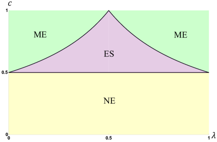
Refer to caption
Figure 4: Entanglement phase diagram for the infinite temperature equilibrated pure state.

4.3 Entanglement phase structure at a finite temperature: general discussion

The infinite temperature case only applies to a system with a finite dimensional Hilbert space at sufficiently high energies or without energy conservation. When the energy of a system is not large enough, or if a system has an infinite dimensional Hilbert space such as in a field theory, energy constraints have to be imposed.

Now there are many more possibilities for ρ(eq)superscript𝜌eq\rho^{\rm(eq)}, which depend on the ensembles we choose and properties of B𝐵B. We may view the different possibilities as giving different universality classes. In this subsection, we summarize the general structure and the main results, leaving explicit discussions of specific choices of ρ(eq)superscript𝜌eq\rho^{\rm(eq)} to subsequent subsections.

At infinite temperature, the Renyi negativities Rnsubscript𝑅𝑛R_{n}, logarithmic negativity {{\mathcal{E}}}, Renyi mutual information Insubscript𝐼𝑛I_{n}, and mutual information I𝐼I all have the same n𝑛n-independent phase structure. At finite temperature, in general each of these infinite number of quantities can give rise to a different phase diagram as a function of the parameters c𝑐c and λ𝜆\lambda defined in (4.2). This reveals intricate patterns of entanglement structure141414Recall that other than the logarithmic negativities, all other quantities are sensitive to classical correlations., but also makes it all but impossible to draw a phase diagram which reflects the behavior of all these quantities. Of particular interest is the behavior of logarithmic negativity {{\mathcal{E}}}, as it directly reflects quantum entanglement correlations, and as reviewed in Sec. 2, can be used to bound the PPT entanglement cost. Furthermore, its relation with mutual information I𝐼I can shed light on the irreversibility of the preparation of a mixed state by different types of operations. A significant technical complication at finite temperature is that the extraction of the logarithmic negativity using analytic continuation becomes a priori unreliable for various parameter ranges due to non-uniform dependence on n𝑛n of Rnsubscript𝑅𝑛R_{n}. The resolvent is needed to calculate {{\mathcal{E}}}, which fortunately can be done for some choices of ρ(eq)superscript𝜌eq\rho^{(\rm eq)} and can be used to illustrate the general structure. Here is a summary of the main features we observe for finite temperature ensembles:

  1. 1.

    As we will discuss immediately below, the mutual information I(A1,A2)𝐼subscript𝐴1subscript𝐴2I(A_{1},A_{2}) has exactly the same phase structure as that at infinite temperature. Thus, the mutual information appears to be insensitive to finite temperature effects.

    The behavior of Renyi mutual informations in general become n𝑛n-dependent, with n𝑛n-dependent phase boundaries. See Fig. 8 for an example.

  2. 2.

    For negativities, each n𝑛n can have its own version of finite-temperature generalizations of the NE, ME, and ES phases, with phase boundaries between them, which in general are n𝑛n-dependent. See Fig. 6 for an example.

  3. 3.

    In the phase diagram of the logarithmic negativity, there are finite-temperature generalizations of the NE, ME and ES phases. Between these phases, there can be new phases that have different {{\mathcal{E}}} behavior, and are separated from other phases by non-analytic dependences on the c,λ𝑐𝜆c,\lambda parameters. Such phases cannot be deduced by analytic continuation of 𝒵n(PT)superscriptsubscript𝒵𝑛PT{\mathcal{Z}}_{n}^{\rm(PT)} or Rnsubscript𝑅𝑛R_{n}. See Fig. 11 for an example.

  4. 4.

    There are regimes where {{\mathcal{E}}} has a nonzero volume-law contribution, but the mutual information I𝐼I is sub-extensive. This is a surprising result, as it is generally believed that mutual information contains both quantum and classical correlations. That it is sub-extensive intuitively implies there cannot be any volume-like quantum entanglement correlations. Our results indicate this intuition cannot be correct. We will elaborate further on this relation between logarithmic negativity and mutual information in Sec. 5.

  5. 5.

    For various choices of ρ(eq)superscript𝜌eq\rho^{(\rm eq)}, the Renyi and logarithmic negativities can often be expressed in terms of equilibrium Renyi entropies, but this appears to not always be the case.

  6. 6.

    Due to the n𝑛n-dependence of phase boundaries of Rnsubscript𝑅𝑛R_{n} and Insubscript𝐼𝑛I_{n}, for a given λ,c𝜆𝑐\lambda,c, there can be intricate patterns of entanglement. For example, it is possible that for all n𝑛n, the negativities show the behavior of the ME phase, while for all n𝑛n the mutual information show the behavior of the ES phase. It can also happen that for different n𝑛n, Rnsubscript𝑅𝑛R_{n} show different phases, i.e. some n𝑛n can be in the ME phase while other n𝑛n are in the ES or NE phases. See Fig. 5 for some examples.

To conclude this general discussion, let us now consider the mutual information. From our general discussion in Sec. 2.3, we have

Sn,A=min(Sn,A(eq),Sn,A¯(eq))subscript𝑆𝑛𝐴minsuperscriptsubscript𝑆𝑛𝐴eqsuperscriptsubscript𝑆𝑛¯𝐴eqS_{n,A}={\rm min}\left(S_{n,A}^{({\rm eq})},S_{n,\bar{A}}^{({\rm eq})}\right)\ (4.24)

for n2𝑛2n\geq 2, as well as

SA=min(SA(eq),SA¯(eq)).subscript𝑆𝐴minsuperscriptsubscript𝑆𝐴eqsuperscriptsubscript𝑆¯𝐴eqS_{A}={\rm min}\left(S_{A}^{({\rm eq})},S_{\bar{A}}^{({\rm eq})}\right)\,. (4.25)

Given that the von Neumann entropy of a thermal density operator is extensive, i.e.

SA1(eq)+SA2(eq)=SA(eq),SA1B(eq)=SA1(eq)+SB(eq),formulae-sequencesuperscriptsubscript𝑆subscript𝐴1eqsuperscriptsubscript𝑆subscript𝐴2eqsuperscriptsubscript𝑆𝐴eqsuperscriptsubscript𝑆subscript𝐴1𝐵eqsuperscriptsubscript𝑆subscript𝐴1eqsuperscriptsubscript𝑆𝐵eqS_{A_{1}}^{({\rm eq})}+S_{A_{2}}^{({\rm eq})}=S_{A}^{({\rm eq})},\quad S_{A_{1}B}^{({\rm eq})}=S_{A_{1}}^{({\rm eq})}+S_{B}^{({\rm eq})}, (4.26)

we then have

I(A1,A2)={0c<12i.e.SA(eq)=SB(eq)SA(eq)SB(eq)c>12, 112c<λ<12c2SA2(eq)λ>12ci.e.SA1(eq)>SA2(eq)+SB(eq)2SA1(eq)λ<112ci.e.SA2(eq)>SA1(eq)+SB(eq)𝐼subscript𝐴1subscript𝐴2cases0𝑐12i.e.superscriptsubscript𝑆𝐴eqsuperscriptsubscript𝑆𝐵eqsuperscriptsubscript𝑆𝐴eqsuperscriptsubscript𝑆𝐵eqformulae-sequence𝑐12112𝑐𝜆12𝑐2superscriptsubscript𝑆subscript𝐴2eq𝜆12𝑐i.e.superscriptsubscript𝑆subscript𝐴1eqsuperscriptsubscript𝑆subscript𝐴2eqsuperscriptsubscript𝑆𝐵eq2superscriptsubscript𝑆subscript𝐴1eq𝜆expectation112𝑐i.e.superscriptsubscript𝑆subscript𝐴2eqsuperscriptsubscript𝑆subscript𝐴1eqsuperscriptsubscript𝑆𝐵eqI(A_{1},A_{2})=\begin{cases}0&c<{{\frac{1}{2}}}\;\;\text{i.e.}\;\;S_{A}^{({\rm eq})}=S_{B}^{(\rm eq)}\cr S_{A}^{({\rm eq})}-S_{B}^{({\rm eq})}&c>{{\frac{1}{2}}},\;1-\frac{1}{2c}<\lambda<\frac{1}{2c}\cr 2S_{A_{2}}^{({\rm eq})}&\lambda>{1\over 2c}\;\;\text{i.e.}\;\;S_{A_{1}}^{({\rm eq})}>S_{A_{2}}^{({\rm eq})}+S_{B}^{(\rm eq)}\cr 2S_{A_{1}}^{({\rm eq})}&\lambda<1-{1\over 2c}\;\;\text{i.e.}\;\;S_{A_{2}}^{({\rm eq})}>S_{A_{1}}^{({\rm eq})}+S_{B}^{(\rm eq)}\end{cases} (4.27)

where c𝑐c and λ𝜆\lambda were defined in (4.2). Thus, we find exactly the same phase structure as that at infinite temperature and the same phase diagram Fig. 4.

For the Renyi mutual information, we have a similar phase structure, but the transitions are in general at n𝑛n-dependent values of c,λ𝑐𝜆c,\lambda. More explicitly, suppose α=ABsubscript𝛼tensor-productsubscript𝐴subscript𝐵{{\mathcal{I}}}_{\alpha}={{\mathcal{I}}}_{A}\otimes{{\mathcal{I}}}_{B} can be factorized between A𝐴A and B𝐵B, then from (4.24),

In(A1,A2)={Sn,A1(eq)+Sn,A2(eq)Sn,A(eq)Sn,A(eq)<Sn,B(eq)Sn,A1(eq)+Sn,A2(eq)Sn,B(eq)Sn,A(eq)>Sn,B(eq),Sn,B(eq)>|Sn,A1(eq)Sn,A2(eq)|2Sn,A2(eq)Sn,A1(eq)>Sn,A2(eq)+Sn,B(eq)2Sn,A1(eq)Sn,A2(eq)>Sn,A1(eq)+Sn,B(eq),subscript𝐼𝑛subscript𝐴1subscript𝐴2casessuperscriptsubscript𝑆𝑛subscript𝐴1eqsuperscriptsubscript𝑆𝑛subscript𝐴2eqsuperscriptsubscript𝑆𝑛𝐴eqsubscriptsuperscript𝑆eq𝑛𝐴subscriptsuperscript𝑆eq𝑛𝐵superscriptsubscript𝑆𝑛subscript𝐴1eqsuperscriptsubscript𝑆𝑛subscript𝐴2eqsuperscriptsubscript𝑆𝑛𝐵eqformulae-sequencesubscriptsuperscript𝑆eq𝑛𝐴subscriptsuperscript𝑆eq𝑛𝐵subscriptsuperscript𝑆eq𝑛𝐵subscriptsuperscript𝑆eq𝑛subscript𝐴1subscriptsuperscript𝑆eq𝑛subscript𝐴22superscriptsubscript𝑆𝑛subscript𝐴2eqsubscriptsuperscript𝑆eq𝑛subscript𝐴1subscriptsuperscript𝑆eq𝑛subscript𝐴2subscriptsuperscript𝑆eq𝑛𝐵2superscriptsubscript𝑆𝑛subscript𝐴1eqsubscriptsuperscript𝑆eq𝑛subscript𝐴2subscriptsuperscript𝑆eq𝑛subscript𝐴1subscriptsuperscript𝑆eq𝑛𝐵I_{n}(A_{1},A_{2})=\begin{cases}S_{n,A_{1}}^{({\rm eq})}+S_{n,A_{2}}^{({\rm eq})}-S_{n,A}^{({\rm eq})}&S^{\rm(eq)}_{n,A}<S^{\rm(eq)}_{n,B}\cr S_{n,A_{1}}^{({\rm eq})}+S_{n,A_{2}}^{({\rm eq})}-S_{n,B}^{({\rm eq})}&S^{\rm(eq)}_{n,A}>S^{\rm(eq)}_{n,B},\;S^{\rm(eq)}_{n,B}>|S^{\rm(eq)}_{n,A_{1}}-S^{\rm(eq)}_{n,A_{2}}|\cr 2S_{n,A_{2}}^{({\rm eq})}&S^{\rm(eq)}_{n,A_{1}}>S^{\rm(eq)}_{n,A_{2}}+S^{\rm(eq)}_{n,B}\cr 2S_{n,A_{1}}^{({\rm eq})}&S^{\rm(eq)}_{n,A_{2}}>S^{\rm(eq)}_{n,A_{1}}+S^{\rm(eq)}_{n,B}\end{cases}, (4.28)

Note that the Renyi entropies from subsystems may not be additive, i.e. Sn,A1(eq)+Sn,A2(eq)superscriptsubscript𝑆𝑛subscript𝐴1eqsuperscriptsubscript𝑆𝑛subscript𝐴2eqS_{n,A_{1}}^{({\rm eq})}+S_{n,A_{2}}^{({\rm eq})} does not have to be equal to Sn,A(eq)superscriptsubscript𝑆𝑛𝐴eqS_{n,A}^{({\rm eq})}.

The behavior of the Renyi and logarithmic negativities is technically much more complicated at finite temperature, and we turn to this next.

4.4 Canonical ensemble

In this subsection, we consider more explicitly the entanglement structure in the canonical ensemble.

4.4.1 General setup

In the canonical ensemble, we consider an effective identity operator of the form

=eβAHAeβBHB,tensor-productsuperscript𝑒subscript𝛽𝐴subscript𝐻𝐴superscript𝑒subscript𝛽𝐵subscript𝐻𝐵{{\mathcal{I}}}=e^{-{\beta}_{A}H_{A}}\otimes e^{-{\beta}_{B}H_{B}}, (4.29)

which can be interpreted in several ways. One possible scenario is that after some brief interactions, subsystems A𝐴A and B𝐵B are separated and thus can achieve separate equilibria at different temperatures. When βA=βB=βsubscript𝛽𝐴subscript𝛽𝐵𝛽{\beta}_{A}={\beta}_{B}={\beta} it also applies to a system AB𝐴𝐵AB with a local Hamiltonian H=HA+HB+HAB𝐻subscript𝐻𝐴subscript𝐻𝐵subscript𝐻𝐴𝐵H=H_{A}+H_{B}+H_{AB} for which eβHeβHAeβHBsuperscript𝑒𝛽𝐻tensor-productsuperscript𝑒𝛽subscript𝐻𝐴superscript𝑒𝛽subscript𝐻𝐵e^{-\beta H}\approx e^{-\beta H_{A}}\otimes e^{-\beta H_{B}}. We can drop the HABsubscript𝐻𝐴𝐵H_{AB} term as it should give contributions proportional to the areas of the subsystems in the exponent, and thus can be neglected in the thermodynamic limit.

We assume that the system is homogeneous within A𝐴A, so that Zm,R=Tr[emβRHR]subscript𝑍𝑚𝑅Trdelimited-[]superscript𝑒𝑚subscript𝛽𝑅subscript𝐻𝑅Z_{m,R}=\text{Tr}[e^{-m\beta_{R}H_{R}}] for different subsystems R𝑅R can be written as

Zm,A1=eVA1fA(mβA),Zm,A2=eVA2fA(mβA),Zm,B=eVBfB(mβB).formulae-sequencesubscript𝑍𝑚subscript𝐴1superscript𝑒subscript𝑉subscript𝐴1subscript𝑓𝐴𝑚subscript𝛽𝐴formulae-sequencesubscript𝑍𝑚subscript𝐴2superscript𝑒subscript𝑉subscript𝐴2subscript𝑓𝐴𝑚subscript𝛽𝐴subscript𝑍𝑚𝐵superscript𝑒subscript𝑉𝐵subscript𝑓𝐵𝑚subscript𝛽𝐵Z_{m,A_{1}}=e^{V_{A_{1}}f_{A}(m\beta_{A})},\quad Z_{m,A_{2}}=e^{V_{A_{2}}f_{A}(m\beta_{A})},\quad Z_{m,B}=e^{V_{B}f_{B}(m\beta_{B})}\ . (4.30)

The corresponding equilibrium Renyi entropy density can be written as

sn,R(eq)(β):=nfR(β)fR(nβ)n1,Sn,R(eq)(β)=VRsn,R(eq)(β).formulae-sequenceassignsubscriptsuperscript𝑠eq𝑛𝑅𝛽𝑛subscript𝑓𝑅𝛽subscript𝑓𝑅𝑛𝛽𝑛1subscriptsuperscript𝑆eq𝑛𝑅𝛽subscript𝑉𝑅subscriptsuperscript𝑠eq𝑛𝑅𝛽s^{\rm(eq)}_{n,R}(\beta):=\frac{nf_{R}(\beta)-f_{R}(n\beta)}{n-1},\qquad S^{\rm(eq)}_{n,R}(\beta)=V_{R}s^{\rm(eq)}_{n,R}(\beta)\ . (4.31)

We allow n𝑛n to take any non-negative real value. The n1𝑛1n\rightarrow 1 limit of (4.31) gives the density of the equilibrium von Neumann entropy (i.e. the thermodynamic entropy density),

sR(eq)(β):=fR(β)βfR(β),SR(eq)(β)=VRsR(eq)(β).formulae-sequenceassignsubscriptsuperscript𝑠eq𝑅𝛽subscript𝑓𝑅𝛽𝛽superscriptsubscript𝑓𝑅𝛽subscriptsuperscript𝑆eq𝑅𝛽subscript𝑉𝑅subscriptsuperscript𝑠eq𝑅𝛽s^{\rm(eq)}_{R}(\beta):=f_{R}(\beta)-\beta f_{R}^{\prime}(\beta),\qquad S^{\rm(eq)}_{R}(\beta)=V_{R}s^{\rm(eq)}_{R}(\beta)\ . (4.32)

The free energy densities fA(β)subscript𝑓𝐴𝛽f_{A}(\beta) and fB(β)subscript𝑓𝐵𝛽f_{B}(\beta) both satisfy the following properties:

  1. 1.

    Since (HHβ)2β=Nf′′(β)subscriptexpectationsuperscript𝐻subscriptexpectation𝐻𝛽2𝛽𝑁superscript𝑓′′𝛽\braket{(H-\braket{H}_{\beta})^{2}}_{\beta}=Nf^{\prime\prime}(\beta) is non-negative,

    f′′(β)0.superscript𝑓′′𝛽0f^{\prime\prime}(\beta)\geq 0. (4.33)
  2. 2.

    From the non-negativity of the thermodynamic entropy,

    f(β)βf(β)0.𝑓𝛽𝛽superscript𝑓𝛽0f(\beta)-\beta f^{\prime}(\beta)\geq 0. (4.34)
  3. 3.

    From the non-negativity of (4.31),

    nf(β)f(nβ)0,n2.formulae-sequence𝑛𝑓𝛽𝑓𝑛𝛽0𝑛2nf(\beta)-f(n\beta)\geq 0,\quad n\geq 2. (4.35)
  4. 4.

    From the fact that sn(eq)superscriptsubscript𝑠𝑛eqs_{n}^{\rm(eq)} decreases with the Renyi index n𝑛n, we have

    ddn(nf(β)f(nβ)n1)0f(β)βf(nβ)f(nβ)nβf(nβ)𝑑𝑑𝑛𝑛𝑓𝛽𝑓𝑛𝛽𝑛10𝑓𝛽𝛽superscript𝑓𝑛𝛽𝑓𝑛𝛽𝑛𝛽superscript𝑓𝑛𝛽\frac{d}{dn}\left(\frac{nf(\beta)-f(n\beta)}{n-1}\right)\leq 0\Rightarrow f(\beta)-\beta f^{\prime}(n\beta)\geq f(n\beta)-n\beta f^{\prime}(n\beta) (4.36)

    Note that (4.36), together with (4.34) at inverse temperature nβ𝑛𝛽n\beta, implies that

    f(β)βf(nβ)0.𝑓𝛽𝛽superscript𝑓𝑛𝛽0f(\beta)-\beta f^{\prime}(n\beta)\geq 0. (4.37)

From (3.4), we find

𝒵n(PT)(A1,A2)=1enFτe𝒜(τ),𝒵n(A)=1enFτe(τ)formulae-sequencesuperscriptsubscript𝒵𝑛(PT)subscript𝐴1subscript𝐴21superscript𝑒𝑛𝐹subscript𝜏superscript𝑒𝒜𝜏superscriptsubscript𝒵𝑛𝐴1superscript𝑒𝑛𝐹subscript𝜏superscript𝑒𝜏{\mathcal{Z}}_{n}^{\text{(PT)}}(A_{1},A_{2})=\frac{1}{e^{nF}}\sum_{\tau}e^{{{\mathcal{A}}}(\tau)},\quad{\mathcal{Z}}_{n}^{(A)}=\frac{1}{e^{nF}}\sum_{\tau}e^{{{\mathcal{B}}}(\tau)} (4.38)

where

𝒜(τ)=VA1i=1k(η1τ)fA(aiβA)+VA2j=1k(ητ)fA(bjβA)+VBk=1k(τ)fB(ckβB),𝒜𝜏subscript𝑉subscript𝐴1superscriptsubscript𝑖1𝑘superscript𝜂1𝜏subscript𝑓𝐴subscript𝑎𝑖subscript𝛽𝐴subscript𝑉subscript𝐴2superscriptsubscript𝑗1𝑘𝜂𝜏subscript𝑓𝐴subscript𝑏𝑗subscript𝛽𝐴subscript𝑉𝐵superscriptsubscript𝑘1𝑘𝜏subscript𝑓𝐵subscript𝑐𝑘subscript𝛽𝐵\displaystyle{{\mathcal{A}}}(\tau)=V_{A_{1}}\sum_{i=1}^{k(\eta^{-1}\tau)}f_{A}(a_{i}\beta_{A})+V_{A_{2}}\sum_{j=1}^{k(\eta\tau)}f_{A}(b_{j}\beta_{A})+V_{B}\sum_{k=1}^{k(\tau)}f_{B}(c_{k}\beta_{B}), (4.39)
(τ)=VAi=1k(η1τ)fA(aiβA)+VBk=1k(τ)fB(ckβB),𝜏subscript𝑉𝐴superscriptsubscript𝑖1𝑘superscript𝜂1𝜏subscript𝑓𝐴subscript𝑎𝑖subscript𝛽𝐴subscript𝑉𝐵superscriptsubscript𝑘1𝑘𝜏subscript𝑓𝐵subscript𝑐𝑘subscript𝛽𝐵\displaystyle{{\mathcal{B}}}(\tau)=V_{A}\sum_{i=1}^{k(\eta^{-1}\tau)}f_{A}(a_{i}\beta_{A})+V_{B}\sum_{k=1}^{k(\tau)}f_{B}(c_{k}\beta_{B}), (4.40)
F=VAfA(βA)+VBfB(βB)𝐹subscript𝑉𝐴subscript𝑓𝐴subscript𝛽𝐴subscript𝑉𝐵subscript𝑓𝐵subscript𝛽𝐵\displaystyle F=V_{A}f_{A}({\beta}_{A})+V_{B}f_{B}({\beta}_{B}) (4.41)

and {ai},{bj},{ck}subscript𝑎𝑖subscript𝑏𝑗subscript𝑐𝑘\{a_{i}\},\{b_{j}\},\{c_{k}\} respectively are the numbers of elements of the cycles in η1τsuperscript𝜂1𝜏\eta^{-1}\tau, ητ𝜂𝜏\eta\tau and τ𝜏\tau. Now if τmsubscript𝜏𝑚\tau_{m} denotes one of the permutations that maximizes 𝒜(τ)𝒜𝜏{{\mathcal{A}}}(\tau) and τmsubscriptsuperscript𝜏𝑚\tau^{\prime}_{m} denotes one of the permutations that maximize (τ)𝜏{{\mathcal{B}}}(\tau) for a particular choice of VA1subscript𝑉subscript𝐴1V_{A_{1}}, VA2subscript𝑉subscript𝐴2V_{A_{2}}, VBsubscript𝑉𝐵V_{B}, then

log𝒵n(PT)(A1,A2)𝒜(τm)nFsuperscriptsubscript𝒵𝑛PTsubscript𝐴1subscript𝐴2𝒜subscript𝜏𝑚𝑛𝐹\log{\mathcal{Z}}_{n}^{(\text{PT})}(A_{1},A_{2})\approx{{\mathcal{A}}}(\tau_{m})-nF (4.42)

and

Rn(A1,A2)=bn(𝒜(τm)(τm))=bn(log𝒵n(PT)log𝒵n(A)).subscript𝑅𝑛subscript𝐴1subscript𝐴2subscript𝑏𝑛𝒜subscript𝜏𝑚subscriptsuperscript𝜏𝑚subscript𝑏𝑛superscriptsubscript𝒵𝑛PTsuperscriptsubscript𝒵𝑛𝐴R_{n}(A_{1},A_{2})=b_{n}\left({{\mathcal{A}}}(\tau_{m})-{{\mathcal{B}}}(\tau^{\prime}_{m})\right)=b_{n}\left(\log{\mathcal{Z}}_{n}^{\rm(PT)}-\log{\mathcal{Z}}_{n}^{(A)}\right)\ . (4.43)

Using the equilibrium Renyi entropies (4.31) we can write the contribution from a permutation τ𝜏\tau to (4.38) as

log𝒵n(PT)(τ)=i=1k(ητ1)(ai1)Sai,A1(eq)+i=1k(ητ)(bi1)Sbi,A2(eq)+i=1k(τ)(ci1)Sci,B(eq)superscriptsubscript𝒵𝑛PT𝜏superscriptsubscript𝑖1𝑘𝜂superscript𝜏1subscript𝑎𝑖1superscriptsubscript𝑆subscript𝑎𝑖subscript𝐴1eqsuperscriptsubscript𝑖1𝑘𝜂𝜏subscript𝑏𝑖1superscriptsubscript𝑆subscript𝑏𝑖subscript𝐴2eqsuperscriptsubscript𝑖1𝑘𝜏subscript𝑐𝑖1superscriptsubscript𝑆subscript𝑐𝑖𝐵eq\displaystyle\log{\mathcal{Z}}_{n}^{\rm(PT)}(\tau)=\sum_{i=1}^{k(\eta\tau^{-1})}-(a_{i}-1)S_{a_{i},A_{1}}^{\rm(eq)}+\sum_{i=1}^{k(\eta\tau)}-(b_{i}-1)S_{b_{i},A_{2}}^{\rm(eq)}+\sum_{i=1}^{k(\tau)}-(c_{i}-1)S_{c_{i},B}^{\rm(eq)} (4.44)
log𝒵n,A(τ)=i=1k(ητ1)(ai1)Sai,A(eq)+i=1k(τ)(ci1)Sci,B(eq)subscript𝒵𝑛𝐴𝜏superscriptsubscript𝑖1𝑘𝜂superscript𝜏1subscript𝑎𝑖1superscriptsubscript𝑆subscript𝑎𝑖𝐴eqsuperscriptsubscript𝑖1𝑘𝜏subscript𝑐𝑖1superscriptsubscript𝑆subscript𝑐𝑖𝐵eq\displaystyle\log{\mathcal{Z}}_{n,A}(\tau)=\sum_{i=1}^{k(\eta\tau^{-1})}-(a_{i}-1)S_{a_{i},A}^{\rm(eq)}+\sum_{i=1}^{k(\tau)}-(c_{i}-1)S_{c_{i},B}^{\rm(eq)} (4.45)

For the Renyi partition function (4.45), the dominant permutations were already reviewed in Sec. 2.3 and the end of last section, given by either τ=e𝜏𝑒\tau=e or τ=η𝜏𝜂\tau=\eta, with

log𝒵n,A(e)=(n1)Sn,A(eq)(βA),log𝒵n,A(η)=(n1)Sn,B(eq)(βB).formulae-sequencesubscript𝒵𝑛𝐴𝑒𝑛1superscriptsubscript𝑆𝑛𝐴eqsubscript𝛽𝐴subscript𝒵𝑛𝐴𝜂𝑛1superscriptsubscript𝑆𝑛𝐵eqsubscript𝛽𝐵\log{\mathcal{Z}}_{n,A}(e)=-(n-1)S_{n,A}^{\rm(eq)}({\beta}_{A}),\quad\log{\mathcal{Z}}_{n,A}(\eta)=-(n-1)S_{n,B}^{\rm(eq)}({\beta}_{B})\ . (4.46)

To find the negativities we need to maximize (4.44) among different permutations τ𝜏\tau, which is a difficult task without knowing the explicit forms of functions fA,fBsubscript𝑓𝐴subscript𝑓𝐵f_{A},f_{B} and relative magnitude of βA,βBsubscript𝛽𝐴subscript𝛽𝐵{\beta}_{A},{\beta}_{B}. We will give detailed discussion for some specific examples and here summarize some general features. In all our investigations we find that for a given n𝑛n, only one of the following set of permutations could dominate: τ=e𝜏𝑒\tau=e, τ=η,η1𝜏𝜂superscript𝜂1\tau=\eta,\eta^{-1}, τ=τES𝜏subscript𝜏𝐸𝑆\tau=\tau_{ES}, which may be considered as giving finite temperature generalizations of the NE, ME and ES phases. The set of τESsubscript𝜏𝐸𝑆\tau_{ES} denotes,

τES={(12)(34)(n1,n) and (23)(45)(n1),evenn{(23)(45)(n1n), (34)(56)(n1),,(12)(n2n1)},oddn,subscript𝜏𝐸𝑆cases1234𝑛1𝑛 and 2345𝑛1even𝑛2345𝑛1𝑛 3456𝑛112𝑛2𝑛1odd𝑛\tau_{ES}=\begin{cases}(12)(34)\cdots(n-1,n)\text{ and }(23)(45)\cdots(n1),&\text{even}\;n\cr\{(23)(45)...(n-1~{}n),$~{} $(34)(56)...(n~{}1),~{}\cdots~{},(12)...(n-2~{}n-1)\},&\text{odd}\;n\end{cases}, (4.47)

which is a subset of the permutations τ,τoddsuperscript𝜏subscriptsuperscript𝜏odd\tau^{\ast},\tau^{\ast}_{\rm odd} for the ES phase at the infinite temperature.151515In some special finite temperature cases, all permutations in the τsuperscript𝜏\tau^{\ast} or τoddsubscriptsuperscript𝜏odd\tau^{\ast}_{\rm odd} give degenerate contributions, but more generally the degeneracy is broken. We note that these permutations are also relevant to the moments of the partial transpose for tensor network states with non-maximally entangled bonds [46]. The corresponding expressions of (4.44) for these permutations are given by

log𝒵n(PT)(e)superscriptsubscript𝒵𝑛PT𝑒\displaystyle\log{\mathcal{Z}}_{n}^{\rm(PT)}(e) =\displaystyle= (n1)Sn,A(eq)(βA)𝑛1superscriptsubscript𝑆𝑛𝐴eqsubscript𝛽𝐴\displaystyle-(n-1)S_{n,A}^{\rm(eq)}({\beta}_{A}) (4.48)
log𝒵n(PT)(η)superscriptsubscript𝒵𝑛PT𝜂\displaystyle\log{\mathcal{Z}}_{n}^{(\text{PT})}(\eta) =\displaystyle= {(n1)Sn,B(eq)(βB)(n2)Sn2,A2(eq)(βA)n2,n even(n1)(Sn,A2(eq)(βA)+Sn,B(eq)(βB))n3,n oddcases𝑛1superscriptsubscript𝑆𝑛𝐵eqsubscript𝛽𝐵𝑛2subscriptsuperscript𝑆eq𝑛2subscript𝐴2subscript𝛽𝐴𝑛2𝑛 even𝑛1superscriptsubscript𝑆𝑛subscript𝐴2eqsubscript𝛽𝐴superscriptsubscript𝑆𝑛𝐵eqsubscript𝛽𝐵𝑛3𝑛 odd\displaystyle\begin{cases}-(n-1)S_{n,B}^{\rm(eq)}({\beta}_{B})-(n-2)S^{(\rm eq)}_{{n\over 2},A_{2}}({\beta}_{A})&n\geq 2,~{}n\text{ even}\\ -(n-1)(S_{n,A_{2}}^{(\rm eq)}({\beta}_{A})+S_{n,B}^{\rm(eq)}({\beta}_{B}))&n\geq 3,~{}n\text{ odd}\end{cases} (4.49)
log𝒵n(PT)(η1)superscriptsubscript𝒵𝑛PTsuperscript𝜂1\displaystyle\log{\mathcal{Z}}_{n}^{(\text{PT})}(\eta^{-1}) =\displaystyle= {(n1)Sn,B(eq)(βB)(n2)Sn2,A1(eq)(βA)n2,n even(n1)(Sn,A1(eq)(βA)+Sn,B(eq)(βB))n3,n oddcases𝑛1superscriptsubscript𝑆𝑛𝐵eqsubscript𝛽𝐵𝑛2subscriptsuperscript𝑆eq𝑛2subscript𝐴1subscript𝛽𝐴𝑛2𝑛 even𝑛1superscriptsubscript𝑆𝑛subscript𝐴1eqsubscript𝛽𝐴superscriptsubscript𝑆𝑛𝐵eqsubscript𝛽𝐵𝑛3𝑛 odd\displaystyle\begin{cases}-(n-1)S_{n,B}^{\rm(eq)}({\beta}_{B})-(n-2)S^{(\rm eq)}_{{n\over 2},A_{1}}({\beta}_{A})&n\geq 2,~{}n\text{ even}\\ -(n-1)(S_{n,A_{1}}^{(\rm eq)}({\beta}_{A})+S_{n,B}^{\rm(eq)}({\beta}_{B}))&n\geq 3,~{}n\text{ odd}\end{cases} (4.50)
log𝒵n(PT)(τES)superscriptsubscript𝒵𝑛PTsubscript𝜏𝐸𝑆\displaystyle\log{\mathcal{Z}}_{n}^{(\text{PT})}(\tau_{ES}) =\displaystyle= {n22Sn2,A(eq)(βA)n2S2,B(eq)(βB)n2,n evenn12(Sn+12,A(eq)(βA)+S2,B(eq)(βB))n3,n odd.cases𝑛22subscriptsuperscript𝑆eq𝑛2𝐴subscript𝛽𝐴𝑛2superscriptsubscript𝑆2𝐵eqsubscript𝛽𝐵𝑛2𝑛 even𝑛12subscriptsuperscript𝑆eq𝑛12𝐴subscript𝛽𝐴superscriptsubscript𝑆2𝐵eqsubscript𝛽𝐵𝑛3𝑛 odd\displaystyle\begin{cases}-{n-2\over 2}S^{\rm(eq)}_{{n\over 2},A}(\beta_{A})-{n\over 2}S_{2,B}^{\rm(eq)}(\beta_{B})&n\geq 2,~{}n\text{ even}\\ -{n-1\over 2}\left(S^{\rm(eq)}_{{n+1\over 2},A}(\beta_{A})+S_{2,B}^{\rm(eq)}({\beta}_{B})\right)&n\geq 3,~{}n\text{ odd}\end{cases}\ . (4.51)

The regions where the different permutations dominate can be found by comparing their magnitudes. For example, for even n𝑛n, τESsubscript𝜏𝐸𝑆\tau_{ES} dominates over e𝑒e when

(n1)Sn,A(eq)n22Sn2,A(eq)n2S2,B(eq)𝑛1superscriptsubscript𝑆𝑛𝐴eq𝑛22superscriptsubscript𝑆𝑛2𝐴eq𝑛2subscriptsuperscript𝑆eq2𝐵(n-1)S_{n,A}^{\rm(eq)}-{n-2\over 2}S_{\frac{n}{2},A}^{\rm(eq)}\geq\frac{n}{2}S^{\rm(eq)}_{2,B} (4.52)

and the equal sign defines the transition line for the change of dominance. These transitions lines are generally n𝑛n-dependent.

If we can analytically continue the expressions (4.48)–(4.51) for even n𝑛n to n=1𝑛1n=1 we would obtain the logarithmic negativity for the corresponding finite temperature generalizations of NE, ME, and ES phases with

NE=0,subscript𝑁𝐸0\displaystyle{{\mathcal{E}}}_{NE}=0, (4.53)
ME=S12,A2(eq)(βA)orME=S12,A1(eq)(βA),formulae-sequencesubscript𝑀𝐸superscriptsubscript𝑆12subscript𝐴2eqsubscript𝛽𝐴orsubscript𝑀𝐸superscriptsubscript𝑆12subscript𝐴1eqsubscript𝛽𝐴\displaystyle{{\mathcal{E}}}_{ME}=S_{{{\frac{1}{2}}},A_{2}}^{\rm(eq)}({\beta}_{A})\quad\text{or}\quad{{\mathcal{E}}}_{ME}=S_{{{\frac{1}{2}}},A_{1}}^{\rm(eq)}({\beta}_{A}), (4.54)
ES=12(S12,A(eq)(βA)S2,B(eq)(βB)).subscript𝐸𝑆12subscriptsuperscript𝑆eq12𝐴subscript𝛽𝐴superscriptsubscript𝑆2𝐵eqsubscript𝛽𝐵\displaystyle{{\mathcal{E}}}_{ES}={{\frac{1}{2}}}\left(S^{\rm(eq)}_{{1\over 2},A}(\beta_{A})-S_{2,B}^{\rm(eq)}(\beta_{B})\right)\ . (4.55)

Comparing with the behavior of mutual information (4.27), notice that in (4.54), S12,A2(eq)(β)subscriptsuperscript𝑆eq12subscript𝐴2𝛽S^{(\rm eq)}_{{1\over 2},A_{2}}({\beta}) appears and is no longer related to the third line of (4.27) by a simple factor of 1212{{\frac{1}{2}}} as it was in the infinite temperature case. Similarly, in (4.55), S12,A(eq)subscriptsuperscript𝑆eq12𝐴S^{(\rm eq)}_{{{\frac{1}{2}}},A} and S2,B(eq)subscriptsuperscript𝑆eq2𝐵S^{(\rm eq)}_{2,B} appear, in contrast to the second line of (4.27). Analytically continuing (4.52) to n=1𝑛1n=1 gives

S12,A(eq)=S2,B(eq)superscriptsubscript𝑆12𝐴eqsubscriptsuperscript𝑆eq2𝐵S_{\frac{1}{2},A}^{\rm(eq)}=S^{\rm(eq)}_{2,B} (4.56)

which may be interpreted as the transition from NE to ES phase for {{\mathcal{E}}}. As we emphasized before, the correctness of such analytic continuations is not warranted in particular in regions of parameters where the dependence on n𝑛n is not uniform. In Sec. 4.4.3 we discuss a case where the resolvent can be calculated numerically, and we checked in the NE and ES regimes that the expressions (4.53), (4.55) and (4.56) do apply.

It is instructive to compare (4.56) with the transition from NE to ES for the mutual information I𝐼I which from (4.27) is given by c=12𝑐12c={{\frac{1}{2}}}, i.e.

SA(eq)=SB(eq).superscriptsubscript𝑆𝐴eqsubscriptsuperscript𝑆eq𝐵S_{A}^{\rm(eq)}=S^{\rm(eq)}_{B}\ . (4.57)

Given that Snsubscript𝑆𝑛S_{n} monotonically decreases with n𝑛n, we have S12,A(eq)>SA(eq)superscriptsubscript𝑆12𝐴eqsuperscriptsubscript𝑆𝐴eqS_{\frac{1}{2},A}^{\rm(eq)}>S_{A}^{\rm(eq)} and S2,B(eq)<SB(eq)subscriptsuperscript𝑆eq2𝐵subscriptsuperscript𝑆eq𝐵S^{\rm(eq)}_{2,B}<S^{\rm(eq)}_{B}, so the transition (4.56) must happen for SA(eq)<SB(eq)superscriptsubscript𝑆𝐴eqsubscriptsuperscript𝑆eq𝐵S_{A}^{\rm(eq)}<S^{\rm(eq)}_{B}, i.e. somewhere with c<12𝑐12c<{{\frac{1}{2}}}. Therefore, (4.56) implies a region in the phase diagram where the logarithmic negativity is extensive, but the mutual information is sub-extensive.

Below, we will consider the following representatives of two classes of examples:

  1. 1.

    In discrete systems, f(β)𝑓𝛽f(\beta) has a well-defined β0𝛽0\beta\rightarrow 0 limit. An example is

    f(β)=log2+logcosh(βJ)𝑓𝛽2𝛽𝐽\quad f(\beta)=\log 2+\log\cosh(\beta J) (4.58)

    which is observed in a variety of spin chain models.

  2. 2.

    In continuum systems, f(β)𝑓𝛽f(\beta) does not have a well-defined β0𝛽0\beta\rightarrow 0 limit. For instance, one form that appears in quantum field theories is

    f(β)=aβα,α0.formulae-sequence𝑓𝛽𝑎superscript𝛽𝛼𝛼0f(\beta)=a\beta^{-\alpha},\quad\alpha\geq 0. (4.59)

4.4.2 A𝐴A and B𝐵B are uniform

As an explicit illustration, we consider the case where the Hamiltonian is translationally invariant and βA=βBsubscript𝛽𝐴subscript𝛽𝐵{\beta}_{A}={\beta}_{B} for which we have fA(β)=fB(β)=f(β)subscript𝑓𝐴𝛽subscript𝑓𝐵𝛽𝑓𝛽f_{A}({\beta})=f_{B}({\beta})=f({\beta}). It will be useful to consider the explicit examples in both (4.58) and (4.59). In this case, it is not clear how to perform a resolvent calculation, so we are not able to find the phase diagram for {{\mathcal{E}}} and will only present the structure for Rnsubscript𝑅𝑛R_{n}.

Since the system is homogeneous, for log𝒵n(A)superscriptsubscript𝒵𝑛𝐴\log{\mathcal{Z}}_{n}^{(A)}, τ=e𝜏𝑒\tau=e dominates for c<12𝑐12c<{{\frac{1}{2}}} and τ=η𝜏𝜂\tau=\eta dominates for c>12𝑐12c>{{\frac{1}{2}}}. In this case, cnsubscript𝑐𝑛c_{n} and λnsubscript𝜆𝑛\lambda_{n} coincide with c𝑐c and λ𝜆\lambda for all n𝑛n, so the Renyi mutual information (4.28) has the same phase structure as the mutual information (4.27).

To understand the structure of log𝒵n(PT)superscriptsubscript𝒵𝑛PT\log{\mathcal{Z}}_{n}^{(\text{PT})}, it is convenient to introduce V=VA+VB𝑉subscript𝑉𝐴subscript𝑉𝐵V=V_{A}+V_{B} and rewrite 𝒜(τ)𝒜𝜏{{\mathcal{A}}}(\tau) in four ways,

1V𝒜(τ)=cλ(G(β,τ)+G(β,η1τ))+c(1λ)(G(β,τ)+G(β,ητ))+(12c)G(β,τ)1𝑉𝒜𝜏𝑐𝜆𝐺𝛽𝜏𝐺𝛽superscript𝜂1𝜏𝑐1𝜆𝐺𝛽𝜏𝐺𝛽𝜂𝜏12𝑐𝐺𝛽𝜏\displaystyle\begin{split}{1\over V}{{\mathcal{A}}}(\tau)=&c\lambda\left(G(\beta,\tau)+G(\beta,\eta^{-1}\tau)\right)+c(1-\lambda)\left(G(\beta,\tau)+G(\beta,\eta\tau)\right)\\ &+(1-2c)G(\beta,\tau)\end{split} (4.60)
=(2cλ1)G(β,η1τ)+c(1λ)(G(β,ητ)+G(β,η1τ))+(1c)(G(β,τ)+G(β,η1τ))absent2𝑐𝜆1𝐺𝛽superscript𝜂1𝜏𝑐1𝜆𝐺𝛽𝜂𝜏𝐺𝛽superscript𝜂1𝜏1𝑐𝐺𝛽𝜏𝐺𝛽superscript𝜂1𝜏\displaystyle\begin{split}=&(2c\lambda-1)G(\beta,\eta^{-1}\tau)+c(1-\lambda)\left(G(\beta,\eta\tau)+G(\beta,\eta^{-1}\tau)\right)\\ &+(1-c)\left(G(\beta,\tau)+G(\beta,\eta^{-1}\tau)\right)\end{split} (4.61)
=cλ(G(β,η1τ)+G(β,ητ))+(2c(1λ)1)G(β,ητ)+(1c)(G(β,τ)+G(β,ητ))absent𝑐𝜆𝐺𝛽superscript𝜂1𝜏𝐺𝛽𝜂𝜏2𝑐1𝜆1𝐺𝛽𝜂𝜏1𝑐𝐺𝛽𝜏𝐺𝛽𝜂𝜏\displaystyle\begin{split}=&c\lambda\left(G(\beta,\eta^{-1}\tau)+G(\beta,\eta\tau)\right)+(2c(1-\lambda)-1)G(\beta,\eta\tau)\\ &+(1-c)\left(G(\beta,\tau)+G(\beta,\eta\tau)\right)\end{split} (4.62)
=(12cλ)(G(β,τ)+G(β,ητ))+(12c(1λ))(G(β,τ)+G(β,η1τ))+(c12)(G(β,ητ)+G(β,η1τ))absent12𝑐𝜆𝐺𝛽𝜏𝐺𝛽𝜂𝜏12𝑐1𝜆𝐺𝛽𝜏𝐺𝛽superscript𝜂1𝜏𝑐12𝐺𝛽𝜂𝜏𝐺𝛽superscript𝜂1𝜏\displaystyle\begin{split}=&(\frac{1}{2}-c\lambda)\left(G(\beta,\tau)+G(\beta,\eta\tau)\right)+(\frac{1}{2}-c(1-\lambda))\left(G(\beta,\tau)+G(\beta,\eta^{-1}\tau)\right)\\ &+(c-\frac{1}{2})\left(G(\beta,\eta\tau)+G(\beta,\eta^{-1}\tau)\right)\end{split} (4.63)

where we have introduced

G(β,τ):=i=1k(τ)f(ciβ)assign𝐺𝛽𝜏superscriptsubscript𝑖1𝑘𝜏𝑓subscript𝑐𝑖𝛽G(\beta,\tau):=\sum_{i=1}^{k(\tau)}f(c_{i}\beta) (4.64)

with {ci}subscript𝑐𝑖\{c_{i}\} the lengths of the cycles in τ𝜏\tau. We show in Appendix D that G(β,τ)𝐺𝛽𝜏G(\beta,\tau) and G(β,η1τ)𝐺𝛽superscript𝜂1𝜏G(\beta,\eta^{-1}\tau) are respectively maximized by τ=e𝜏𝑒\tau=e and τ=η𝜏𝜂\tau=\eta, and G(β,τ)+G(β,η1τ)𝐺𝛽𝜏𝐺𝛽superscript𝜂1𝜏G(\beta,\tau)+G(\beta,\eta^{-1}\tau) is maximized by both τ=e𝜏𝑒\tau=e and τ=η𝜏𝜂\tau=\eta. Similarly, G(β,ητ)𝐺𝛽𝜂𝜏G(\beta,\eta\tau) is maximized by τ=η1𝜏superscript𝜂1\tau=\eta^{-1}, and G(β,τ)+G(β,ητ)𝐺𝛽𝜏𝐺𝛽𝜂𝜏G(\beta,\tau)+G(\beta,\eta\tau) is maximized by both τ=e𝜏𝑒\tau=e and τ=η1𝜏superscript𝜂1\tau=\eta^{-1}. Furthermore, we observe numerically that G(β,ητ)+G(β,η1τ)𝐺𝛽𝜂𝜏𝐺𝛽superscript𝜂1𝜏G(\beta,\eta\tau)+G(\beta,\eta^{-1}\tau) is maximized for even n𝑛n by four permutations: τ=η,η1𝜏𝜂superscript𝜂1\tau=\eta,\eta^{-1} and τES={(12)(34)(n1n),(23)(45)(n1)}subscript𝜏𝐸𝑆1234𝑛1𝑛2345𝑛1\tau_{ES}=\{(12)(34)...(n-1~{}n),~{}(23)(45)...(n1)\}, and for odd n𝑛n by two permutations: τ=η,η1𝜏𝜂superscript𝜂1\tau=\eta,\eta^{-1}.

From the above, we then find:

  1. 1.

    For c<12𝑐12c<\frac{1}{2}, from (4.60) τ=e𝜏𝑒\tau=e is the dominant permutation for 𝒜(τ)𝒜𝜏{{\mathcal{A}}}(\tau) for all n3𝑛3n\geq 3, with log𝒵n(PT)superscriptsubscript𝒵𝑛PT\log{\mathcal{Z}}_{n}^{(\text{PT})} given by (4.48). Since τ=e𝜏𝑒\tau=e is also the dominant permutation for (τ)𝜏{{\mathcal{B}}}(\tau), we have

    Rn(A1,A2)=0,n3,limn2Rn(A1,A2)=0,\begin{gathered}R_{n}(A_{1},A_{2})=0,\quad n\geq 3,\quad\quad\lim_{n\rightarrow 2}R_{n}(A_{1},A_{2})=0,\end{gathered} (4.65)

    This is the natural generalization of the NE phase for the Rnsubscript𝑅𝑛R_{n}.

  2. 2.

    For c>12,λ>12cformulae-sequence𝑐12𝜆12𝑐c>{{\frac{1}{2}}},~{}\lambda>\frac{1}{2c}, from (4.61) the dominant permutation for 𝒜(τ)𝒜𝜏{{\mathcal{A}}}(\tau) is η𝜂\eta, with log𝒵n(PT)superscriptsubscript𝒵𝑛PT\log{\mathcal{Z}}_{n}^{(\text{PT})} given by (4.49) and

    Rn(A1,A2)={VA2nf(β)f(nβ)n1=Sn,A2(eq)n3,n oddVA2nf(β)2f(n2β)n2=Sn2,A2(eq)n4,n evensubscript𝑅𝑛subscript𝐴1subscript𝐴2casessubscript𝑉subscript𝐴2𝑛𝑓𝛽𝑓𝑛𝛽𝑛1subscriptsuperscript𝑆eq𝑛subscript𝐴2𝑛3𝑛 oddsubscript𝑉subscript𝐴2𝑛𝑓𝛽2𝑓𝑛2𝛽𝑛2subscriptsuperscript𝑆eq𝑛2subscript𝐴2𝑛4𝑛 even\displaystyle R_{n}(A_{1},A_{2})=\begin{cases}V_{A_{2}}\frac{nf(\beta)-f(n\beta)}{n-1}=S^{(\rm eq)}_{n,A_{2}}&n\geq 3,n\text{ odd}\\ V_{A_{2}}\frac{nf(\beta)-2f(\frac{n}{2}\beta)}{n-2}=S^{(\rm eq)}_{{n\over 2},A_{2}}&n\geq 4,n\text{ even}\end{cases} (4.66)
    limn2Rn(A1,A2)=SA2(eq)(β),subscript𝑛2subscript𝑅𝑛subscript𝐴1subscript𝐴2subscriptsuperscript𝑆eqsubscript𝐴2𝛽\displaystyle\lim_{n\rightarrow 2}R_{n}(A_{1},A_{2})=S^{\rm(eq)}_{A_{2}}(\beta), (4.67)

    From analytic continuation, {{\mathcal{E}}} is given by (4.54). This may naturally be interpreted as the finite temperature generalization of the maximally entangled (ME) phase. Notice in (4.66) for even n𝑛n, Sn2,A2(eq)(β)subscriptsuperscript𝑆eq𝑛2subscript𝐴2𝛽S^{(\rm eq)}_{{n\over 2},A_{2}}({\beta}) appears instead of Sn,A2(eq)(β)subscriptsuperscript𝑆eq𝑛subscript𝐴2𝛽S^{(\rm eq)}_{n,A_{2}}({\beta}) as in the third line of (4.28) for Renyi mutual information.

    For c>12,λ<112cformulae-sequence𝑐12𝜆112𝑐c>{{\frac{1}{2}}},\lambda<1-\frac{1}{2c}, the dominant permutation is η1superscript𝜂1\eta^{-1}, and we get similar expressions with A2subscript𝐴2A_{2} replaced by A1subscript𝐴1A_{1}.

  3. 3.

    For c>1/2𝑐12c>1/2, 112c<λ<12c112𝑐𝜆12𝑐1-\frac{1}{2c}<\lambda<\frac{1}{2c}, the dominant permutations now appear to depend on values of c𝑐c and λ𝜆\lambda, and are model-dependent. We present the phase diagrams for examples (4.58) and (4.59) based on the behavior of even n𝑛n in Fig. 5 (a) and (b) respectively. In addition to the NE and ME phases discussed in items 1 and 2 above, there are also the following regions in the phase diagrams:
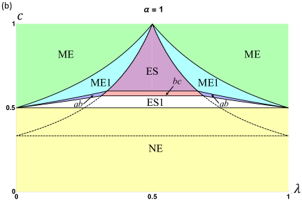
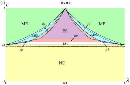
    Refer to caption
    Refer to caption
    Figure 5: Phase diagrams for the canonical ensemble in a homogeneous system. (a) shows the case with f(β)𝑓𝛽f(\beta) as in (4.58), and (b) shows the case with f(β)𝑓𝛽f(\beta) in (4.59). Note that in (a), in addition to the ab𝑎𝑏ab, bc𝑏𝑐bc and ac𝑎𝑐ac regions, there is also a small abc𝑎𝑏𝑐abc region near the intersections of these regions which is not shown explicitly in the figure. The dashed lines show the prediction for the phase transition in the logarithmic negativity from the naive analytic continuation prescription, where we set ES=NEsubscript𝐸𝑆subscript𝑁𝐸{{\mathcal{E}}}_{ES}={{\mathcal{E}}}_{NE} or ES=MEsubscript𝐸𝑆subscript𝑀𝐸{{\mathcal{E}}}_{ES}={{\mathcal{E}}}_{ME} in (4.53)-(4.55).
    1. (a)

      ME1 region in Fig. 5 where τm=ηsubscript𝜏𝑚𝜂\tau_{m}=\eta or τm=η1subscript𝜏𝑚superscript𝜂1\tau_{m}=\eta^{-1} dominates for all n𝑛n. The behavior of Renyi and logarithmic negativities are the same as (4.66) and (4.54). But note that the mutual information in this region are given by the second line of (4.27) rather than the third line or fourth line. So the mutual information and Renyi mutual information in this region differ from those of ME in item 2, and they should be considered as describing distinct phases. We refer to this region as the ME1 phase. It is curious that in this region, the negativities behave like those in the maximally entangled phase, while the mutual informations behave like those for the entanglement saturation phase. In contrast to the relation (2.25) for pure states, we have for even n𝑛n

      Rn(A1,A2)>12In/2(A1,A2).subscript𝑅𝑛subscript𝐴1subscript𝐴212subscript𝐼𝑛2subscript𝐴1subscript𝐴2R_{n}(A_{1},A_{2})>\frac{1}{2}I_{n/2}(A_{1},A_{2})\ . (4.68)
    2. (b)

      ES1 region in Fig. 5 where τm=esubscript𝜏𝑚𝑒\tau_{m}=e dominates for all n3𝑛3n\geq 3. But since for c>12𝑐12c>{{\frac{1}{2}}} the dominant permutation for (τ)𝜏{{\mathcal{B}}}(\tau) is τ=η𝜏𝜂\tau=\eta, the values of Rnsubscript𝑅𝑛R_{n} are different from those in (4.65),

      Rn(A1,A2)={n1n2(Sn,A(eq)Sn,B(eq))nevenSn,A(eq)Sn,B(eq)nodd,n3formulae-sequencesubscript𝑅𝑛subscript𝐴1subscript𝐴2cases𝑛1𝑛2superscriptsubscript𝑆𝑛𝐴eqsubscriptsuperscript𝑆eq𝑛𝐵𝑛evensuperscriptsubscript𝑆𝑛𝐴eqsubscriptsuperscript𝑆eq𝑛𝐵𝑛odd𝑛3\displaystyle R_{n}(A_{1},A_{2})=\begin{cases}{n-1\over n-2}(S_{n,A}^{(\rm eq)}-S^{\rm(eq)}_{n,B})&n\,{\rm even}\cr S_{n,A}^{(\rm eq)}-S^{\rm(eq)}_{n,B}&n\,{\rm odd}\end{cases},\quad n\geq 3\ (4.69)
      log𝒵n(PT)={(n1)Sn,A(eq)n3S2,B(eq)n=2.superscriptsubscript𝒵𝑛PTcases𝑛1superscriptsubscript𝑆𝑛𝐴eq𝑛3subscriptsuperscript𝑆eq2𝐵𝑛2\displaystyle\log{\mathcal{Z}}_{n}^{\rm(PT)}=\begin{cases}-(n-1)S_{n,A}^{(\rm eq)}&n\geq 3\\ -S^{\rm(eq)}_{2,B}&n=2\end{cases}\ . (4.70)

      We cannot obtain (A1,A2)subscript𝐴1subscript𝐴2{{\mathcal{E}}}(A_{1},A_{2}) by analytic continuation from the above expressions, as the analytical continuation of (4.70) for even n4𝑛4n\geq 4 to n=2𝑛2n=2 already gives the wrong expression, not to mention to n=1𝑛1n=1. The mutual information of this region is given by the second line of (4.27), which is also nonzero. So this should describe a distinct phase from the NE phase of item 1. Since  (4.69)–(4.70) and the Renyi mutual informations in this phase only depend on A𝐴A, and not on A1,A2subscript𝐴1subscript𝐴2A_{1},A_{2}, we will refer to it as the ES1 phase. For n=2𝑛2n=2, there is no ES1 region.

    3. (c)

      ES region in Fig. 5 where τm=τESsubscript𝜏𝑚subscript𝜏𝐸𝑆\tau_{m}=\tau_{ES} for all n𝑛n with log𝒵n(PT)superscriptsubscript𝒵𝑛PT\log{\mathcal{Z}}_{n}^{(\text{PT})} given by (4.51). We find

      Rn(A1,A2)={12Sn12,A(eq)(β)Sn,B(eq)(β)+12S2,B(eq)(β)n3,n odd12(Sn2,A(eq)(β)Sn2,B(eq)(2β))n4,n evensubscript𝑅𝑛subscript𝐴1subscript𝐴2cases12subscriptsuperscript𝑆eq𝑛12𝐴𝛽subscriptsuperscript𝑆eq𝑛𝐵𝛽12subscriptsuperscript𝑆eq2𝐵𝛽𝑛3𝑛 odd12subscriptsuperscript𝑆eq𝑛2𝐴𝛽subscriptsuperscript𝑆eq𝑛2𝐵2𝛽𝑛4𝑛 even\displaystyle R_{n}(A_{1},A_{2})=\begin{cases}{{\frac{1}{2}}}S^{\rm(eq)}_{{n-1\over 2},A}(\beta)-S^{\rm(eq)}_{n,B}({\beta})+{{\frac{1}{2}}}S^{\rm(eq)}_{2,B}({\beta})&n\geq 3,n\text{ odd}\\ \frac{1}{2}(S^{\rm(eq)}_{{n\over 2},A}(\beta)-S^{\rm(eq)}_{{n\over 2},B}(2\beta))&n\geq 4,n\text{ even}\end{cases} (4.71)
      limn2Rn(A1,A2)=12SA(eq)(β)12SB(eq)(2β)subscript𝑛2subscript𝑅𝑛subscript𝐴1subscript𝐴212superscriptsubscript𝑆𝐴eq𝛽12subscriptsuperscript𝑆eq𝐵2𝛽\displaystyle\lim_{n\rightarrow 2}R_{n}(A_{1},A_{2})={{\frac{1}{2}}}S_{A}^{(\rm eq)}({\beta})-{{\frac{1}{2}}}S^{\rm(eq)}_{B}(2{\beta}) (4.72)

      and the logarithmic negativity is given by (4.55). Notice all quantities depend only on properties of A𝐴A, not on A1subscript𝐴1A_{1} or A2subscript𝐴2A_{2}. We can thus identity this as the finite temperature generalization of the ES phase. For even n𝑛n we also have (4.68).

    4. (d)

      In the remaining regions of Fig. 5, the set of dominant permutations now depends on n𝑛n. For example, in the region denoted by ac𝑎𝑐ac there exists a critical value ncsubscript𝑛𝑐n_{c} for nnc𝑛subscript𝑛𝑐n\leq n_{c}, the dominant permutations are that of item (a), while for n>nc𝑛subscript𝑛𝑐n>n_{c}, the dominant permutations are those of item (c). Similarly with bc𝑏𝑐bc and ab𝑎𝑏ab regions. There is in general also an abc𝑎𝑏𝑐abc region where all three options appear at a given c,λ𝑐𝜆c,\lambda for different n𝑛n. These regions also give potentially new phases. Clearly in these “mixed” regions, there is no way to perform analytic continuation in n𝑛n to obtain (A1,A2)subscript𝐴1subscript𝐴2{{\mathcal{E}}}(A_{1},A_{2}).

      In the above, we have assumed that for a region if a given set of permutations dominate for all n𝑛n and there is no apparent contradiction, we can analytically continue n𝑛n to obtain the logarithmic negativity. But we should caution that it is not warranted such a procedure always gives the correct answer.

  4. 4.

    As the temperature decreases, the ES phase region shrinks.

The n𝑛n-dependent transition lines for Rnsubscript𝑅𝑛R_{n} are shown for a few examples of even and odd n𝑛n in Figs. 6 and 7. Fig. 6 shows the case of f(β)𝑓𝛽f(\beta) as in (4.58), at two different values of β𝛽\beta. Fig. 7 shows the case of f(β)𝑓𝛽f(\beta) in (4.59), where the transition lines turn out to be independent of β𝛽\beta, at two different values of the parameter α𝛼\alpha. Note that there are qualitative differences between the diagrams for even and odd n𝑛n. In particular, for sufficiently large β𝛽\beta or α𝛼\alpha, the odd n𝑛n cases have no region where τESsubscript𝜏𝐸𝑆\tau_{ES} dominates.

Refer to caption
Refer to caption
Refer to caption
Refer to caption
Figure 6: Transition lines for Rnsubscript𝑅𝑛R_{n} at two different values of β𝛽\beta for f(β)𝑓𝛽f(\beta) in (4.58).
Refer to caption
Refer to caption
Refer to caption
Refer to caption
Figure 7: Transition lines for Rnsubscript𝑅𝑛R_{n} at two different values of α𝛼\alpha for f(β)𝑓𝛽f(\beta) in (4.59).

4.4.3 A𝐴A at infinite temperature

As another illustration, here we consider the case where A𝐴A is at infinite temperature, while B𝐵B is at a finite temperature β𝛽{\beta}. We find numerically for n=4,6𝑛46n=4,6 that the transition the dominant permutation contributing to 𝒵n(PT)superscriptsubscript𝒵𝑛PT{\mathcal{Z}}_{n}^{\rm(PT)} is always one out of e𝑒e, τsuperscript𝜏\tau^{\ast}, and η,η1𝜂superscript𝜂1\eta,\eta^{-1}, and assume that this is true for all n𝑛n. The corresponding expressions for 𝒵n(PT)superscriptsubscript𝒵𝑛PT{\mathcal{Z}}_{n}^{\rm(PT)} and analytically continued expressions for {{\mathcal{E}}} are given by (4.48)-(4.51) and (4.53)-(4.55). The phase transitions for both the mutual information and the Renyi negativities are nlimit-from𝑛n-dependent in this case, and are shown in Fig. 8.

These phase diagrams have a similar structure for both discrete and continuum examples (4.58) and (4.59). The phase diagrams for both Rnsubscript𝑅𝑛R_{n} and Insubscript𝐼𝑛I_{n} are n𝑛n-dependent in this case. However, the transition from dominance of τ=e𝜏𝑒\tau=e to τ=τES𝜏subscript𝜏𝐸𝑆\tau=\tau_{ES} for all Rnsubscript𝑅𝑛R_{n} happens along the same line, indicated as the purple dashed line in the figure. This coincides with the transition in I2subscript𝐼2I_{2} from NE to ES, and takes place at a smaller value of c𝑐c than the corresponding transition in I𝐼I. As explained in Appendix C.3, the transition in {{\mathcal{E}}} obtained from the semicircle approximation in the resolvent also lies along the same line. More explicitly, in the semi-circle approximation, the logarithmic negativity is given by

(A1,A2)subscript𝐴1subscript𝐴2\displaystyle{\cal E}(A_{1},A_{2}) =log(2πsin1[12eS2,B(eq)dA]+(eS2,B(eq)dA+8dAeS2,B(eq))114eS2,B(eq)dA3π),absent2𝜋superscript112superscript𝑒subscriptsuperscript𝑆eq2𝐵subscript𝑑𝐴superscript𝑒subscriptsuperscript𝑆eq2𝐵subscript𝑑𝐴8subscript𝑑𝐴superscript𝑒subscriptsuperscript𝑆eq2𝐵114superscript𝑒subscriptsuperscript𝑆eq2𝐵subscript𝑑𝐴3𝜋\displaystyle=\log\left(\frac{2}{\pi}\sin^{-1}\left[{{\frac{1}{2}}}\sqrt{\frac{e^{S^{\rm(eq)}_{2,B}}}{d_{A}}}\,\right]+\frac{\left(\sqrt{\frac{e^{S^{\rm(eq)}_{2,B}}}{d_{A}}}+8\sqrt{\frac{d_{A}}{e^{S^{\rm(eq)}_{2,B}}}}\right)\sqrt{1-\frac{1}{4}{\frac{e^{S^{\rm(eq)}_{2,B}}}{d_{A}}}}}{3\pi}\right), (4.73)
{0,logdA<S2,B(eq)12(logdAS2,B(eq))+log83π,logdA>S2,B(eq)similar-to-or-equalsabsentcases0subscript𝑑𝐴subscriptsuperscript𝑆eq2𝐵12subscript𝑑𝐴subscriptsuperscript𝑆eq2𝐵83𝜋subscript𝑑𝐴subscriptsuperscript𝑆eq2𝐵\displaystyle\simeq\begin{cases}0,&\log d_{A}<S^{\rm(eq)}_{2,B}\\ \frac{1}{2}\left(\log d_{A}-S^{\rm(eq)}_{2,B}\right)+\log\frac{8}{3\pi},&\log d_{A}>S^{\rm(eq)}_{2,B}\end{cases} (4.74)

Comparison between the mutual information and negativity is shown in Fig. 9. Here, we explicit see a regime before the Page time when the negativity is extensive and hence much larger than the mutual information.
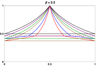
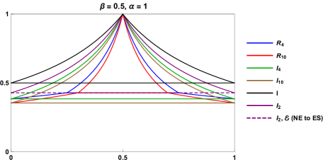
Refer to caption
Refer to caption
Figure 8: Phase transition lines for Rnsubscript𝑅𝑛R_{n} and Insubscript𝐼𝑛I_{n} for a few different n𝑛n for fBsubscript𝑓𝐵f_{B} as in (4.58) and (4.59) are shown on the left and right respectively.
Refer to caption
Figure 9: The mutual information (blue), negativity (orange), von Neumann entropy of R𝑅R (green), and second Rényi entropy of R𝑅R (red) are shown when B𝐵B is in the canonical ensemble and A𝐴A at infinite temperature. While the mutual information within A𝐴A becomes volume-law when the von Neumann entropy of A𝐴A saturates, the negativity becomes volume-law when the second Rényi entropy saturates, a significantly earlier time. We also note that the finite temperature corrections around the transition point are significantly larger for the mutual information than they are for negativity, which has a sharper transition. We take VB=100subscript𝑉𝐵100V_{B}=100 and β=1/2𝛽12\beta=1/2 for a Cardy-like density of states for B𝐵B, ρ(E)=eVBEVB𝜌𝐸superscript𝑒subscript𝑉𝐵𝐸subscript𝑉𝐵\rho(E)=e^{V_{B}\sqrt{\frac{E}{V_{B}}}}.

4.5 Microcanonical ensemble

4.5.1 General description

In cases where the initial state is supported on a narrow interval IE,Δ=[EΔ,E+Δ]subscript𝐼𝐸Δ𝐸Δ𝐸ΔI_{E,\Delta}=[E-\Delta,E+\Delta] of energies, we can take the effective identity operator for the equilibrium approximation to be the projector onto the eigenstates in this microcanonical interval. Again assuming that the interaction terms between different subsystems A1,A2subscript𝐴1subscript𝐴2A_{1},A_{2} and B𝐵B give small contributions to the energy compared to the terms involving only degrees of freedom within the subsystems, we can approximate this effective identity operator as

E=EnIE,Δ|nn|EpA1+EqA2+ErBIE,Δ(|pp|)A1(|qq|)A2(|rr|)B.subscript𝐸subscriptsubscript𝐸𝑛subscript𝐼𝐸Δket𝑛bra𝑛subscriptsuperscriptsubscript𝐸𝑝subscript𝐴1superscriptsubscript𝐸𝑞subscript𝐴2superscriptsubscript𝐸𝑟𝐵subscript𝐼𝐸Δtensor-productsubscriptket𝑝bra𝑝subscript𝐴1subscriptket𝑞bra𝑞subscript𝐴2subscriptket𝑟bra𝑟𝐵{{\mathcal{I}}}_{E}=\sum_{E_{n}\in I_{E,\Delta}}\ket{n}\bra{n}\approx\sum_{E_{p}^{A_{1}}+E_{q}^{A_{2}}+E_{r}^{B}\in I_{E,\Delta}}(\ket{p}\bra{p})_{A_{1}}\otimes(\ket{q}\bra{q})_{A_{2}}\otimes(\ket{r}\bra{r})_{B}. (4.75)

where |p,|qket𝑝ket𝑞\ket{p},\ket{q} and |rket𝑟\ket{r} are respectively eigenstates of HA1subscript𝐻subscript𝐴1H_{A_{1}}, HA2subscript𝐻subscript𝐴2H_{A_{2}} and HBsubscript𝐻𝐵H_{B} with energies EpA1superscriptsubscript𝐸𝑝subscript𝐴1E_{p}^{A_{1}}, EqA2superscriptsubscript𝐸𝑞subscript𝐴2E_{q}^{A_{2}} and ErBsuperscriptsubscript𝐸𝑟𝐵E_{r}^{B}. Below we will denote NE:=Tr[E]assignsubscript𝑁𝐸Trdelimited-[]subscript𝐸N_{E}:=\text{Tr}[{{\mathcal{I}}}_{E}]. The contributions to the equilibrium approximation for 𝒵n(PT)superscriptsubscript𝒵𝑛PT{\mathcal{Z}}_{n}^{(\rm PT)} from general permutations τ𝜏\tau with this choice of αsubscript𝛼{{\mathcal{I}}}_{\alpha} in a general homogenous system are complicated to evaluate, and in particular do not have simple expressions in terms of the cycle numbers and lengths of various permutations like the canonical ensemble expressions (4.38). Some examples are shown in Appendix E. We consider two simplifying cases below, with B𝐵B or A2subscript𝐴2A_{2} at infinite temperature. These examples are useful as they allow a calculation of the logarithmic negativity through the resolvent, as explained in Appendices C.4 and C.5, revealing new features in their phase diagrams which do not have an analog at infinite temperature and cannot be deduced from the phase diagrams for the Renyi negativities. In both examples, we find that the logarithmic negativity becomes extensive in a regime where the mutual information is sub-extensive.

For concreteness, in both cases below, it will sometimes be useful to consider a specific example of the entropy density as a function of energy density in the part of the system with energy conservation,

s(ϵ)=gϵ.𝑠italic-ϵ𝑔italic-ϵs(\epsilon)=g\sqrt{\epsilon}. (4.76)

where g𝑔g is a constant.

4.5.2 B𝐵B at infinite temperature

Let us first assume that the total energy in A𝐴A is conserved and it equilibrates to the microcanonical ensemble, while B𝐵B equilibrates to infinite temperature. The effective identity operator is

α=Ea1A1+Ea2A2IE,Δ|a1a1||a2a2|𝟏Bsubscript𝛼subscriptsubscriptsuperscript𝐸subscript𝐴1subscript𝑎1subscriptsuperscript𝐸subscript𝐴2subscript𝑎2subscript𝐼𝐸Δtensor-producttensor-productketsubscript𝑎1brasubscript𝑎1ketsubscript𝑎2brasubscript𝑎2subscript1𝐵{{\mathcal{I}}}_{{\alpha}}=\sum_{E^{A_{1}}_{a_{1}}+E^{A_{2}}_{a_{2}}\in I_{E,\Delta}}\ket{a_{1}}\bra{a_{1}}\otimes\ket{a_{2}}\bra{a_{2}}\otimes\mathbf{1}_{B} (4.77)

As we vary the volumes of the different subsystems, we fix the average energy density in A𝐴A to a value EVA=ϵ𝐸subscript𝑉𝐴italic-ϵ\frac{E}{V_{A}}=\epsilon, and the infinite temperature entropy density in B𝐵B to a value s0subscript𝑠0s_{0}.

Note first that since αsubscript𝛼{{\mathcal{I}}}_{{\alpha}} factorizes as ABtensor-productsubscript𝐴subscript𝐵{{\mathcal{I}}}_{A}\otimes{{\mathcal{I}}}_{B} in this example, the Renyi mutual information is again given by the general expression (4.28). Note that Sn,A(eq)subscriptsuperscript𝑆eq𝑛𝐴S^{\rm(eq)}_{n,A} and Sn,B(eq)subscriptsuperscript𝑆eq𝑛𝐵S^{\rm(eq)}_{n,B} for all n𝑛n in this example are equal to SA(eq)subscriptsuperscript𝑆eq𝐴S^{\rm(eq)}_{A} and SB(eq)=logdBsubscriptsuperscript𝑆eq𝐵subscript𝑑𝐵S^{\rm(eq)}_{B}=\log d_{B} respectively, so the transition from the first to the second line of (4.28) occurs at SA(eq)=logdBsubscriptsuperscript𝑆eq𝐴subscript𝑑𝐵S^{\rm(eq)}_{A}=\log d_{B} for all n𝑛n. But note that in this example, the first line of (4.28) is not zero for n1𝑛1n\neq 1: it is positive for n<1𝑛1n<1, and negative for n>1𝑛1n>1.

The contributions to 𝒵n(PT)superscriptsubscript𝒵𝑛PT{\mathcal{Z}}_{n}^{\rm(PT)} for even n2𝑛2n\geq 2 from different permutations are

log𝒵n(PT)(e)superscriptsubscript𝒵𝑛PT𝑒\displaystyle\log{\mathcal{Z}}_{n}^{\rm(PT)}(e) =\displaystyle= (n1)SA(eq)𝑛1superscriptsubscript𝑆𝐴eq\displaystyle-(n-1)S_{A}^{\rm(eq)} (4.78)
log𝒵n(PT)(η)superscriptsubscript𝒵𝑛PT𝜂\displaystyle\log{\mathcal{Z}}_{n}^{(\text{PT})}(\eta) =\displaystyle= (n1)logdB(n2)Sn2,A2(eq)𝑛1subscript𝑑𝐵𝑛2subscriptsuperscript𝑆eq𝑛2subscript𝐴2\displaystyle-(n-1)\log d_{B}-(n-2)S^{(\rm eq)}_{{n\over 2},A_{2}} (4.79)
log𝒵n(PT)(η1)superscriptsubscript𝒵𝑛PTsuperscript𝜂1\displaystyle\log{\mathcal{Z}}_{n}^{(\text{PT})}(\eta^{-1}) =\displaystyle= (n1)logdB(n2)Sn2,A1(eq)𝑛1subscript𝑑𝐵𝑛2subscriptsuperscript𝑆eq𝑛2subscript𝐴1\displaystyle-(n-1)\log d_{B}-(n-2)S^{(\rm eq)}_{{n\over 2},A_{1}} (4.80)
log𝒵n(PT)(τES)superscriptsubscript𝒵𝑛PTsubscript𝜏𝐸𝑆\displaystyle\log{\mathcal{Z}}_{n}^{(\text{PT})}(\tau_{ES}) =\displaystyle= n22Sn2,A1(eq)n22Sn2,A2(eq)n2logdB𝑛22subscriptsuperscript𝑆eq𝑛2subscript𝐴1𝑛22subscriptsuperscript𝑆eq𝑛2subscript𝐴2𝑛2subscript𝑑𝐵\displaystyle-{n-2\over 2}S^{\rm(eq)}_{{n\over 2},A_{1}}-{n-2\over 2}S^{\rm(eq)}_{{n\over 2},A_{2}}-{n\over 2}\log d_{B} (4.81)

The derivation of these expressions is explained in Appendix C.4. On noticing that Sn,A(eq)=SA(eq)subscriptsuperscript𝑆eq𝑛𝐴subscriptsuperscript𝑆eq𝐴S^{\rm(eq)}_{n,A}=S^{\rm(eq)}_{A} and Sn,B(eq)=logdBsubscriptsuperscript𝑆eq𝑛𝐵subscript𝑑𝐵S^{\rm(eq)}_{n,B}=\log d_{B} for all n𝑛n in this example, and that the equilibrium Renyi entropies of different subsystems are additive in the canonical ensemble, we can see that these expressions in terms of the equilibrium entropies turn out to be the same as the contributions from the leading permutations in the canonical ensemble case, (4.48)-(4.51). From analytic continuation, the above expressions correspond to the following values of the logarithmic negativity:

NE=0,subscript𝑁𝐸0\displaystyle{{\mathcal{E}}}_{NE}=0, (4.82)
ME=S12,A2(eq)orME=S12,A1(eq),formulae-sequencesubscript𝑀𝐸superscriptsubscript𝑆12subscript𝐴2eqorsubscript𝑀𝐸superscriptsubscript𝑆12subscript𝐴1eq\displaystyle{{\mathcal{E}}}_{ME}=S_{{{\frac{1}{2}}},A_{2}}^{\rm(eq)}\quad\text{or}\quad{{\mathcal{E}}}_{ME}=S_{{{\frac{1}{2}}},A_{1}}^{\rm(eq)}, (4.83)
ES=12(S12,A1(eq)+S12,A2(eq)logdB).subscript𝐸𝑆12subscriptsuperscript𝑆eq12subscript𝐴1subscriptsuperscript𝑆eq12subscript𝐴2subscript𝑑𝐵\displaystyle{{\mathcal{E}}}_{ES}={{\frac{1}{2}}}\left(S^{\rm(eq)}_{{1\over 2},A_{1}}+S^{\rm(eq)}_{{1\over 2},A_{2}}-\log d_{B}\right)\ . (4.84)

Depending on the permutations τmsubscript𝜏𝑚\tau_{m} and τmsubscriptsuperscript𝜏𝑚\tau^{\prime}_{m} that dominate in 𝒵n(PT)superscriptsubscript𝒵𝑛PT{\mathcal{Z}}_{n}^{\rm(PT)} and 𝒵n(A)superscriptsubscript𝒵𝑛𝐴{\mathcal{Z}}_{n}^{(A)} respectively, the Renyi negativities for even n𝑛n can take three possible forms,

Rn={0τm=e,τm=emin(Sn2,A2eq,Sn2,A1eq)τm=η1,η,τm=η12(Sn/2,A1eq+Sn/2,A1eqlogdB)τm=τES,τm=ηsubscript𝑅𝑛cases0formulae-sequencesubscript𝜏𝑚𝑒superscriptsubscript𝜏𝑚𝑒minsubscriptsuperscript𝑆eq𝑛2subscript𝐴2subscriptsuperscript𝑆eq𝑛2subscript𝐴1formulae-sequencesubscript𝜏𝑚superscript𝜂1𝜂superscriptsubscript𝜏𝑚𝜂12subscriptsuperscript𝑆eq𝑛2subscript𝐴1subscriptsuperscript𝑆eq𝑛2subscript𝐴1subscript𝑑𝐵formulae-sequencesubscript𝜏𝑚subscript𝜏𝐸𝑆superscriptsubscript𝜏𝑚𝜂R_{n}=\begin{cases}0&\tau_{m}=e,~{}\tau_{m}^{\prime}=e\\ \text{min}(S^{\rm eq}_{\frac{n}{2},A_{2}},S^{\rm eq}_{\frac{n}{2},A_{1}})&\tau_{m}=\eta^{-1},\eta,~{}\tau_{m}^{\prime}=\eta\\ \frac{1}{2}(S^{\rm eq}_{n/2,A_{1}}+S^{\rm eq}_{n/2,A_{1}}-\log d_{B})&\tau_{m}=\tau_{ES},~{}\tau_{m}^{\prime}=\eta\end{cases} (4.85)

Note that this example does not have an ES1 phase like (4.69) where τm=e,τm=ηformulae-sequencesubscript𝜏𝑚𝑒superscriptsubscript𝜏𝑚𝜂\tau_{m}=e,~{}\tau_{m}^{\prime}=\eta for n>2𝑛2n>2.

Refer to caption
Figure 10: Phase transition lines for Rnsubscript𝑅𝑛R_{n} and Insubscript𝐼𝑛I_{n} for n=4,10𝑛410n=4,10. The transition from NE to ES for {{\mathcal{E}}} obtained from the semi-circle approximation is shown with the dashed purple line. The transition from the first to the second line of (4.28) for all Renyi mutual informations coincides with the black n=1𝑛1n=1 transition line in this case.

The n𝑛n-dependent phase transition lines for Rnsubscript𝑅𝑛R_{n} and Insubscript𝐼𝑛I_{n} are shown in Fig. 10, taking the entropy density in A𝐴A to be of the form (4.76). Analytic continuation of the condition 𝒵n(PT)(τES)=𝒵n(PT)(e)superscriptsubscript𝒵𝑛PTsubscript𝜏𝐸𝑆superscriptsubscript𝒵𝑛PT𝑒{\mathcal{Z}}_{n}^{(\text{PT})}(\tau_{ES})={\mathcal{Z}}_{n}^{(\text{PT})}(e) suggests that the transition from the NE to the ES phase for the logarithmic negativity takes place when

S1/2,A1(eq)+S1/2,A2(eq)=logdB.subscriptsuperscript𝑆eq12subscript𝐴1subscriptsuperscript𝑆eq12subscript𝐴2subscript𝑑𝐵S^{\rm(eq)}_{1/2,A_{1}}+S^{\rm(eq)}_{1/2,A_{2}}=\log d_{B}\,. (4.86)

This analytically continued phase transition line is indicated with the dashed purple line in Fig. 10. When this transition takes place, the mutual information is still sub-extensive from (4.27). As discussed in Appendix C.4, a computation of the resolvent in the “semicircle approximation” for this case indicates that the naive analytic continuation of the phase transition (4.86), and the analytically continued value (4.84) of the logarithmic negativity in the ES phase, are correct. However, our computation of the full resolvent in a different setup in the following subsection suggests that the semicircle approximation may in principle be insensitive to new phases that cannot be deduced by analytic continuation. Irrespective of whether such new phases also exist in this example, the conclusion that the negativity is extensive in a regime where the mutual information is sub-extensive holds.

4.5.3 A2subscript𝐴2A_{2} at infinite temperature

Consider an inhomogeneous example, where the system A2subscript𝐴2A_{2} is taken to be at infinite temperature while A1Bsubscript𝐴1𝐵A_{1}B is a homogenous system that satisfies energy conservation and equilibrates to the microcanonical ensemble. More explicitly, we take the effective identity operator to be

α=𝟏A2EpA1+ErBIE,Δ(|pp|)A1(|rr|)B.subscript𝛼tensor-productsubscript1subscript𝐴2subscriptsuperscriptsubscript𝐸𝑝subscript𝐴1superscriptsubscript𝐸𝑟𝐵subscript𝐼𝐸Δtensor-productsubscriptket𝑝bra𝑝subscript𝐴1subscriptket𝑟bra𝑟𝐵{{\mathcal{I}}}_{\alpha}=\mathbf{1}_{A_{2}}\otimes\sum_{E_{p}^{A_{1}}+E_{r}^{B}\in I_{E,\Delta}}(\ket{p}\bra{p})_{A_{1}}\otimes(\ket{r}\bra{r})_{B}. (4.87)

As we vary the volumes of the different subsystems to find the phase diagram, we keep the average energy density in A1Bsubscript𝐴1𝐵A_{1}B fixed to some value EVA1+VB=ϵ𝐸subscript𝑉subscript𝐴1subscript𝑉𝐵italic-ϵ\frac{E}{V_{A_{1}}+V_{B}}=\epsilon. We denote the infinite temperature equilibrium entropy density in A2subscript𝐴2A_{2} by s0subscript𝑠0s_{0}.

Using (2.48), we find that the Renyi mutual informations in this setup are given by

In(A1,A2)={0Sn,A1(eq)+logdA2<Sn,B(eq)Sn,A1(eq)+logdA2Sn,B(eq),Sn,A1(eq)+logdA2>Sn,B(eq),Sn,A1(eq)<logdA2+Sn,B(eq),logdA2<Sn,A1B(eq)2logdA2logdA2>Sn,A1B(eq)Sn,A1(eq)+Sn,A1B(eq)Sn,B(eq)Sn,A1(eq)>logdA2+Sn,B(eq)subscript𝐼𝑛subscript𝐴1subscript𝐴2cases0subscriptsuperscript𝑆eq𝑛subscript𝐴1subscript𝑑subscript𝐴2subscriptsuperscript𝑆eq𝑛𝐵subscriptsuperscript𝑆eq𝑛subscript𝐴1subscript𝑑subscript𝐴2subscriptsuperscript𝑆eq𝑛𝐵formulae-sequencesubscriptsuperscript𝑆eq𝑛subscript𝐴1subscript𝑑subscript𝐴2subscriptsuperscript𝑆eq𝑛𝐵subscriptsuperscript𝑆eq𝑛subscript𝐴1subscript𝑑subscript𝐴2subscriptsuperscript𝑆eq𝑛𝐵otherwisesubscript𝑑subscript𝐴2subscriptsuperscript𝑆eq𝑛subscript𝐴1𝐵2subscript𝑑subscript𝐴2subscript𝑑subscript𝐴2subscriptsuperscript𝑆eq𝑛subscript𝐴1𝐵superscriptsubscript𝑆𝑛subscript𝐴1eqsuperscriptsubscript𝑆𝑛subscript𝐴1𝐵eqsuperscriptsubscript𝑆𝑛𝐵eqsubscriptsuperscript𝑆eq𝑛subscript𝐴1subscript𝑑subscript𝐴2subscriptsuperscript𝑆eq𝑛𝐵I_{n}(A_{1},A_{2})=\begin{cases}0&S^{\rm(eq)}_{n,A_{1}}+\log d_{A_{2}}<S^{\rm(eq)}_{n,B}\\ S^{\rm(eq)}_{n,A_{1}}+\log d_{A_{2}}-S^{\rm(eq)}_{n,B},&S^{\rm(eq)}_{n,A_{1}}+\log d_{A_{2}}>S^{\rm(eq)}_{n,B},~{}S^{\rm(eq)}_{n,A_{1}}<\log d_{A_{2}}+S^{\rm(eq)}_{n,B},\\ &\log d_{A_{2}}<S^{\rm(eq)}_{n,A_{1}B}\\ 2\log d_{A_{2}}&\log d_{A_{2}}>S^{\rm(eq)}_{n,A_{1}B}\\ S_{n,A_{1}}^{\rm(eq)}+S_{n,A_{1}B}^{\rm(eq)}-S_{n,B}^{\rm(eq)}&S^{\rm(eq)}_{n,A_{1}}>\log d_{A_{2}}+S^{\rm(eq)}_{n,B}\end{cases} (4.88)

Note that this differs slightly from (4.28), as the Renyi entropies for n1𝑛1n\neq 1 in A1Bsubscript𝐴1𝐵A_{1}B are not additive in this example. For I(A1,A2)𝐼subscript𝐴1subscript𝐴2I(A_{1},A_{2}), we recover the general expression (4.27). The phase transitions for different Insubscript𝐼𝑛I_{n} are n𝑛n-dependent in this example.

We find that the dominant permutation in 𝒵n(PT)superscriptsubscript𝒵𝑛PT{\mathcal{Z}}_{n}^{\rm(PT)} for even n𝑛n is given by one of the choices τ=e𝜏𝑒\tau=e, τ=η,η1𝜏𝜂superscript𝜂1\tau=\eta,\eta^{-1} or τ=τES𝜏subscript𝜏𝐸𝑆\tau=\tau_{ES} 161616We checked this numerically for n=4𝑛4n=4 and n=6𝑛6n=6 for the entropy density function in (4.76)., and the corresponding values are

logZn(PT)(e)superscriptsubscript𝑍𝑛PT𝑒\displaystyle\log Z_{n}^{\rm(PT)}(e) =(1n)(logdA2+Sn,A1(eq)),absent1𝑛subscript𝑑subscript𝐴2superscriptsubscript𝑆𝑛subscript𝐴1eq\displaystyle=(1-n)\,(\log d_{A_{2}}+S_{n,A_{1}}^{\rm(eq)}), (4.89)
logZn(PT)(η1)superscriptsubscript𝑍𝑛PTsuperscript𝜂1\displaystyle\log Z_{n}^{\rm(PT)}(\eta^{-1}) =S12,A1(eq)(n1)(SB(eq)+SA1(eq)),absentsubscriptsuperscript𝑆eq12subscript𝐴1𝑛1subscriptsuperscript𝑆eq𝐵subscriptsuperscript𝑆eqsubscript𝐴1\displaystyle=S^{\rm(eq)}_{{{\frac{1}{2}}},A_{1}}-(n-1)(S^{\rm(eq)}_{B}+S^{\rm(eq)}_{A_{1}}), (4.90)
logZn(PT)(η)superscriptsubscript𝑍𝑛PT𝜂\displaystyle\log Z_{n}^{\rm(PT)}(\eta) =(2n)logdA2+(1n)SB,n(eq),absent2𝑛subscript𝑑subscript𝐴21𝑛superscriptsubscript𝑆𝐵𝑛eq\displaystyle=(2-n)\log d_{A_{2}}+(1-n)S_{B,n}^{\rm(eq)}, (4.91)
logZn(PT)(τES)superscriptsubscript𝑍𝑛PTsubscript𝜏𝐸𝑆\displaystyle\log Z_{n}^{\rm(PT)}(\tau_{ES}) =(1n2)logdA2+Snn+2,A1(eq)n2(SA1(eq)+SB(eq)).absent1𝑛2subscript𝑑subscript𝐴2subscriptsuperscript𝑆eq𝑛𝑛2subscript𝐴1𝑛2subscriptsuperscript𝑆eqsubscript𝐴1subscriptsuperscript𝑆eq𝐵\displaystyle=(1-\frac{n}{2})\log d_{A_{2}}+S^{\rm(eq)}_{\frac{n}{n+2},A_{1}}-\frac{n}{2}(S^{\rm(eq)}_{A_{1}}+S^{\rm(eq)}_{B}). (4.92)

From analytic continuation of the above expressions, we get the following forms of the logarithmic negativity:

NE=0,subscript𝑁𝐸0\displaystyle{{\mathcal{E}}}_{NE}=0, (4.93)
ME=logdA2orME=S12,A1(eq),formulae-sequencesubscript𝑀𝐸subscript𝑑subscript𝐴2orsubscript𝑀𝐸superscriptsubscript𝑆12subscript𝐴1eq\displaystyle{{\mathcal{E}}}_{ME}=\log d_{A_{2}}\quad\text{or}\quad{{\mathcal{E}}}_{ME}=S_{{{\frac{1}{2}}},A_{1}}^{\rm(eq)}, (4.94)
ES=12logdA2+S13,A1(eq)12SA1(eq)12SB(eq).subscript𝐸𝑆12subscript𝑑subscript𝐴2subscriptsuperscript𝑆eq13subscript𝐴112subscriptsuperscript𝑆eqsubscript𝐴112superscriptsubscript𝑆𝐵eq\displaystyle{{\mathcal{E}}}_{ES}={{\frac{1}{2}}}\log d_{A_{2}}+S^{\rm(eq)}_{{1\over 3},A_{1}}-{{\frac{1}{2}}}S^{\rm(eq)}_{A_{1}}-{{\frac{1}{2}}}S_{B}^{\rm(eq)}\ . (4.95)

We also find the following different forms of the Renyi negativities for even n𝑛n depending on the permutations τmsubscript𝜏𝑚\tau_{m} and τmsuperscriptsubscript𝜏𝑚\tau_{m}^{\prime} that dominate in 𝒵n(PT)superscriptsubscript𝒵𝑛PT{\mathcal{Z}}_{n}^{\rm(PT)} and 𝒵n(A)superscriptsubscript𝒵𝑛𝐴{\mathcal{Z}}_{n}^{(A)} respectively:

Rn(A1,A2)={0τm=e,τm=en1n2(Sn,A(eq)Sn,A)τm=e,τm=η12logdA2+n2(n2)(SA1(eq)+SB(eq))1n2Snn+2,A1(eq)n1n2Sn,B(eq)τm=η1,τm=ηSA2(eq)τm=η,τm=η(n1)S1/n,A1(eq)S1/2,A1(eq)n2τm=τES,τm=ηsubscript𝑅𝑛subscript𝐴1subscript𝐴2cases0formulae-sequencesubscript𝜏𝑚𝑒superscriptsubscript𝜏𝑚𝑒𝑛1𝑛2subscriptsuperscript𝑆eq𝑛𝐴subscript𝑆𝑛𝐴formulae-sequencesubscript𝜏𝑚𝑒superscriptsubscript𝜏𝑚𝜂12subscript𝑑subscript𝐴2𝑛2𝑛2subscriptsuperscript𝑆eqsubscript𝐴1subscriptsuperscript𝑆eq𝐵otherwise1𝑛2subscriptsuperscript𝑆eq𝑛𝑛2subscript𝐴1𝑛1𝑛2subscriptsuperscript𝑆eq𝑛𝐵formulae-sequencesubscript𝜏𝑚superscript𝜂1superscriptsubscript𝜏𝑚𝜂subscriptsuperscript𝑆eqsubscript𝐴2formulae-sequencesubscript𝜏𝑚𝜂superscriptsubscript𝜏𝑚𝜂𝑛1subscriptsuperscript𝑆eq1𝑛subscript𝐴1subscriptsuperscript𝑆eq12subscript𝐴1𝑛2formulae-sequencesubscript𝜏𝑚subscript𝜏𝐸𝑆superscriptsubscript𝜏𝑚𝜂R_{n}(A_{1},A_{2})=\begin{cases}\vspace{0.2cm}0&\tau_{m}=e,~{}\tau_{m}^{\prime}=e\\ \vspace{0.2cm}\frac{n-1}{n-2}(S^{\rm(eq)}_{n,A}-S_{n,A})&\tau_{m}=e,~{}\tau_{m}^{\prime}=\eta\\ \frac{1}{2}\log d_{A_{2}}+\frac{n}{2(n-2)}(S^{\rm(eq)}_{A_{1}}+S^{\rm(eq)}_{B})&{}\textstyle\\ \vspace{0.2cm}-\frac{1}{n-2}S^{\rm(eq)}_{\frac{n}{n+2},\,A_{1}}-\frac{n-1}{n-2}S^{\rm(eq)}_{n,B}&\tau_{m}=\eta^{-1},~{}\tau_{m}^{\prime}=\eta\\ \vspace{0.2cm}S^{\rm(eq)}_{A_{2}}&\tau_{m}=\eta,~{}\tau_{m}^{\prime}=\eta\\ \frac{(n-1)S^{\rm(eq)}_{1/n,A_{1}}-S^{\rm(eq)}_{1/2,A_{1}}}{n-2}&\tau_{m}=\tau_{ES},~{}\tau_{m}^{\prime}=\eta\end{cases} (4.96)

The phase transition lines for Rnsubscript𝑅𝑛R_{n} and Insubscript𝐼𝑛I_{n} for n=4,6𝑛46n=4,6 and 888 are shown in Fig. 11(a), where we have assumed that the entropy density in A1Bsubscript𝐴1𝐵A_{1}B is given by (4.76). Qualitatively, this has a similar structure to the phase diagrams seen in previous cases, with analogs of each of the regions NE, ES1, ES, ME1, ME, ab𝑎𝑏ab, bc𝑏𝑐bc, ac𝑎𝑐ac and abc𝑎𝑏𝑐abc that we saw previously.

Refer to caption
Refer to caption
Figure 11: (a) shows the phases of {{\mathcal{E}}} with αsubscript𝛼{{\mathcal{I}}}_{{\alpha}} as in (4.87), s(ϵ)=ϵ𝑠italic-ϵitalic-ϵs(\epsilon)=\sqrt{\epsilon} in A1Bsubscript𝐴1𝐵A_{1}B, and EV=0.5𝐸𝑉0.5\frac{E}{V}=0.5. The phase transitions of the mutual information are shown with dashed black lines. In (b), we show the same phase transition lines of {{\mathcal{E}}} alongside the phase transition lines of 𝒵n(PT)superscriptsubscript𝒵𝑛PT{\mathcal{Z}}_{n}^{\rm(PT)} for n=4,6,8𝑛468n=4,6,8. Note that the precise shape of all phase transition lines will depend on the choices of s(ϵ)𝑠italic-ϵs(\epsilon) and EV𝐸𝑉\frac{E}{V}.

For this example, we are further able to use the resolvent to find the full phase diagram of the logarithmic negativity. We present the details of this calculation in Appendix C.5. The resulting phase digram is shown in Fig. 11(b). Each of the five different shaded regions, labelled NE, ES, ME, ES-ME1 and ES-ME2, represents a distinct phase of the logarithmic negativity. The phase transition lines for the mutual information are also shown in the same figure with dashed lines, but the corresponding regions are not shaded. In the top row of Fig. 12, both {{\mathcal{E}}} and I𝐼I are shown as functions of the parameter c=SA(eq)SA(eq)+SB(eq)𝑐subscriptsuperscript𝑆eq𝐴subscriptsuperscript𝑆eq𝐴subscriptsuperscript𝑆eq𝐵c=\frac{S^{\rm(eq)}_{A}}{S^{\rm(eq)}_{A}+S^{\rm(eq)}_{B}} along different vertical lines marked in the phase diagram of Fig. 11(b), which have different fixed values of the ratio λ=SA1(eq)SA(eq)𝜆subscriptsuperscript𝑆eqsubscript𝐴1subscriptsuperscript𝑆eq𝐴\lambda=\frac{S^{\rm(eq)}_{A_{1}}}{S^{\rm(eq)}_{A}}. The various phases shown in the diagram should be interpreted as follows:

  1. 1.

    In the phases labelled by NE, ES, and ME, {{\mathcal{E}}} is given by the analytically continued expressions (4.93)-(4.95).

  2. 2.

    In the phases labelled by ES-ME1 and ES-ME2, {{\mathcal{E}}} cannot be obtained by analytic continuation of 𝒵n(PT)superscriptsubscript𝒵𝑛PT{\mathcal{Z}}_{n}^{\rm(PT)} or {{\mathcal{E}}}. The expressions for the negativity in these phases are given respectively by

    ESME1=SA2(eq)+VA1(s(θ3)s(ϵ))VBs(ϵ).subscript𝐸𝑆𝑀𝐸1subscriptsuperscript𝑆eqsubscript𝐴2subscript𝑉subscript𝐴1𝑠subscript𝜃3𝑠italic-ϵsubscript𝑉𝐵𝑠italic-ϵ{{\mathcal{E}}}_{ES-ME1}=S^{\rm(eq)}_{A_{2}}+V_{A_{1}}(s(\theta_{3})-s(\epsilon))-V_{B}s(\epsilon)\,. (4.97)

    and

    ESME2=VA1(2s(θ2)s(ϵ))VBs(ϵ).subscript𝐸𝑆𝑀𝐸2subscript𝑉subscript𝐴12𝑠subscript𝜃2𝑠italic-ϵsubscript𝑉𝐵𝑠italic-ϵ{{\mathcal{E}}}_{ES-ME2}=V_{A_{1}}\,(2s(\theta_{2})-s(\epsilon))-V_{B}\,s(\epsilon)\,. (4.98)

    where θ2subscript𝜃2\theta_{2} and θ3subscript𝜃3\theta_{3} are solutions to the equations

    VA2s0+VBs(ϵ(VA1+VB)VA1θ2VB)=VA1s(θ2),VA1s(θ3)+VBs(ϵ(VA1+VB)VA1θ3VB)=VA2s0.formulae-sequencesubscript𝑉subscript𝐴2subscript𝑠0subscript𝑉𝐵𝑠italic-ϵsubscript𝑉subscript𝐴1subscript𝑉𝐵subscript𝑉subscript𝐴1subscript𝜃2subscript𝑉𝐵subscript𝑉subscript𝐴1𝑠subscript𝜃2subscript𝑉subscript𝐴1𝑠subscript𝜃3subscript𝑉𝐵𝑠italic-ϵsubscript𝑉subscript𝐴1subscript𝑉𝐵subscript𝑉subscript𝐴1subscript𝜃3subscript𝑉𝐵subscript𝑉subscript𝐴2subscript𝑠0\begin{gathered}V_{A_{2}}\,s_{0}+V_{B}\,s\left(\frac{\epsilon\,(V_{A_{1}}+V_{B})-V_{A_{1}}\,\theta_{2}}{V_{B}}\right)=V_{A_{1}}s(\theta_{2}),\\ V_{A_{1}}\,s(\theta_{3})+V_{B}\,s\left(\frac{\epsilon\,(V_{A_{1}}+V_{B})-V_{A_{1}}\,\theta_{3}}{V_{B}}\right)=V_{A_{2}}s_{0}\,.\end{gathered} (4.99)
  3. 3.

    Only one of the phase transition lines shown in the figure – the pink line dividing the NE and ES phases – can be correctly deduced by naive analytic continuation. Putting n=1𝑛1n=1 in the condition Zn(PT)(τES)Zn(PT)(e)superscriptsubscript𝑍𝑛PTsubscript𝜏𝐸𝑆superscriptsubscript𝑍𝑛PT𝑒Z_{n}^{\rm(PT)}(\tau_{ES})\geq Z_{n}^{\rm(PT)}(e), we would deduce that the transition line between the NE and ES phases for {{\mathcal{E}}} is given by

    12SA2eq+S1/3,A1eq12SA1eq12SBeq=012superscriptsubscript𝑆subscript𝐴2eqsuperscriptsubscript𝑆13subscript𝐴1eq12superscriptsubscript𝑆subscript𝐴1eq12subscriptsuperscript𝑆eq𝐵0\frac{1}{2}S_{A_{2}}^{\rm eq}+S_{1/3,A_{1}}^{\rm eq}-\frac{1}{2}S_{A_{1}}^{\rm eq}-\frac{1}{2}S^{\rm eq}_{B}=0 (4.100)

    (4.100) agrees with the pink line in Fig 11(b), but it cannot be used to determine the point where the pink line ends and the cyan line begins, as the naive analytic continuation does not “know about” the existence of the ES-ME2 phase. The semi-circle approximation for the resolvent in this example also correctly predicts the pink line for the transition from NE to ES, but is again insensitive to the ES-ME2 phase.

  4. 4.

    In the transition from NE to ES or ES-ME2, there is a discontinuity in the first derivative of {{\mathcal{E}}} with respect to c𝑐c. The remaining phase transitions correspond to a discontinuity in the second derivative. We show c𝑐\frac{\partial{{\mathcal{E}}}}{\partial c} along different vertical lines in the phase diagram in the bottom row of Fig. 12. This is unlike the infinite temperature case, where all phase transitions involve discontinuities in the first derivative of {{\mathcal{E}}}.

  5. 5.

    In the region between the dashed black line and the pink and cyan lines, the mutual information is sub-extensive while the negativity is extensive. Comparing (4.100) with the NE to ES transition line for the mutual information in (4.57), we see quite generally that since S1/3,A1(eq)>SA1(eq)subscriptsuperscript𝑆eq13subscript𝐴1subscriptsuperscript𝑆eqsubscript𝐴1S^{\rm(eq)}_{1/3,A_{1}}>S^{\rm(eq)}_{A_{1}}, such a regime should exist for any choice of s(ϵ)𝑠italic-ϵs(\epsilon), as long as the naive transition line for the logarithmic negativity in (4.100) is correct.

    Note also that the NE-ES transition line for I1/2subscript𝐼12I_{1/2} lies slightly below, but quite close to, that of the mutual information. In particular, it also lies above the lines where the logarithmic negativity starts to become extensive.
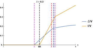
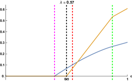
Refer to caption
Refer to caption
Refer to caption
Refer to caption
Refer to caption
Refer to caption
Figure 12: Top row: the blue and orange curves respectively show {{\mathcal{E}}} and I𝐼I as a function of c𝑐c along three vertical lines in the phase diagram of Fig. 11(b). Bottom row: c𝑐\frac{\partial{{\mathcal{E}}}}{\partial c} is shown along the same lines. The relevant phase transitions lines from Fig. 11(b) are also indicated with dashed vertical lines.

4.6 Numerical examples: negativity spectrum in chaotic spin chains

Throughout this work, we have used an analytic approximation that holds in the thermodynamic limit to calculate various information-theoretic quantities. In this subsection, we present results for the spectrum of the partially transposed density matrix in the canonical ensemble. Here we avoid all approximations and carry out numerical simulations in chaotic spin chains, but are necessarily limited to small sizes.

We consider a chaotic 1D spin chain with Hamiltonian

H=i=1N(ZiZi+1+hxXi+hzZi).𝐻superscriptsubscript𝑖1𝑁subscript𝑍𝑖subscript𝑍𝑖1subscript𝑥subscript𝑋𝑖subscript𝑧subscript𝑍𝑖\displaystyle H=-\sum_{i=1}^{N}\left(Z_{i}Z_{i+1}+h_{x}X_{i}+h_{z}Z_{i}\right). (4.101)

This Hamiltonian has been studied frequently as it undergoes a well-understood integrable to chaotic transition [47]. We find, numerically, that this model has the following partition function

g(β)=logZ(β)N=log(2cosh(f(hx,hz)β))𝑔𝛽𝑍𝛽𝑁2𝑓subscript𝑥subscript𝑧𝛽\displaystyle g(\beta)=\frac{\log Z(\beta)}{N}=\log\left(2\cosh\left(f(h_{x},h_{z})\beta\right)\right) (4.102)

to extremely precise accuracy. Here, there is only a single fitting parameter, f𝑓f, that depends on the coupling constants chosen. This can be fixed by the low-temperature behavior of the partition function

logZ(β)N=βE0N=βf(hx,hz).𝑍𝛽𝑁𝛽subscript𝐸0𝑁𝛽𝑓subscript𝑥subscript𝑧\displaystyle\frac{\log Z(\beta\rightarrow\infty)}{N}=-\frac{\beta E_{0}}{N}=\beta f(h_{x},h_{z}). (4.103)

Thus, we have

g(β)=log(2cosh(ε0β)),𝑔𝛽2subscript𝜀0𝛽\displaystyle g(\beta)=\log\left(2\cosh\left(\varepsilon_{0}\beta\right)\right), (4.104)

where ε0subscript𝜀0\varepsilon_{0} is the ground state energy density. We set hx=1.05subscript𝑥1.05h_{x}=-1.05 and hz=0.5subscript𝑧0.5h_{z}=0.5 in our calculations below.

If we want to model the canonical ensemble, it is convenient to study the “canonical thermal pure quantum states” of Ref. [48]

|βeβH/2|R,proportional-toket𝛽superscript𝑒𝛽𝐻2ket𝑅\displaystyle\ket{\beta}\propto e^{-\beta H/2}\ket{R}, (4.105)

where |Rket𝑅\ket{R} is a random state vector. Being random, it is approximately an equal weighting of all energy eigenstates

|β1Z(β)EneβEn/2|En.similar-to-or-equalsket𝛽1𝑍𝛽subscriptsubscript𝐸𝑛superscript𝑒𝛽subscript𝐸𝑛2ketsubscript𝐸𝑛\displaystyle\ket{\beta}\simeq\frac{1}{\sqrt{Z(\beta)}}\sum_{E_{n}}e^{-\beta E_{n}/2}\ket{E_{n}}. (4.106)

The exponential of the Hamiltonian is a dense matrix, so a priori, we will be very limited in the system sizes. This can be improved by approximating the exponential as

eβH/2eβ(HA𝟙B)/2eβ(𝟙AHB)/2,similar-to-or-equalssuperscript𝑒𝛽𝐻2superscript𝑒𝛽tensor-productsubscript𝐻𝐴subscript1𝐵2superscript𝑒𝛽tensor-productsubscript1𝐴subscript𝐻𝐵2\displaystyle e^{-\beta H/2}\simeq e^{-\beta(H_{A}\otimes\mathbbm{1}_{B})/2}e^{-\beta(\mathbbm{1}_{A}\otimes H_{B})/2}, (4.107)

where, as in the equilibrium approximation, we have considered the coupling HABsubscript𝐻𝐴𝐵H_{AB} to be small. A Haar random vector can be written as [49]

|R=iαXiα|iA|αB,ket𝑅subscript𝑖𝛼tensor-productsubscript𝑋𝑖𝛼subscriptket𝑖𝐴subscriptket𝛼𝐵\displaystyle\ket{R}=\sum_{i\alpha}X_{i\alpha}\ket{i}_{A}\otimes\ket{\alpha}_{B}, (4.108)

where the Xiαsubscript𝑋𝑖𝛼X_{i\alpha}’s are independent complex Gaussian random variables and |i,|αket𝑖ket𝛼\ket{i},\ket{\alpha} are orthonormal bases on the sub-Hilbert spaces. The (unnormalized) reduced density matrix on subsystem A𝐴A may then by expressed as

ρA(β)=eβHA/2XXeβHA/2,subscript𝜌𝐴𝛽superscript𝑒𝛽subscript𝐻𝐴2𝑋superscript𝑋superscript𝑒𝛽subscript𝐻𝐴2\displaystyle\rho_{A}(\beta)=e^{-\beta H_{A}/2}XX^{*}e^{-\beta H_{A}/2}, (4.109)

where X𝑋X is now the dA×dBsubscript𝑑𝐴subscript𝑑𝐵d_{A}\times d_{B} rectangular matrix with matrix elements Xiαsubscript𝑋𝑖𝛼X_{i\alpha}. This is a great numerical simplification because we avoid ever forming dense, (dAdB)×(dAdB)subscript𝑑𝐴subscript𝑑𝐵subscript𝑑𝐴subscript𝑑𝐵(d_{A}d_{B})\times(d_{A}d_{B}) matrices.

In Fig. 13, we show the exact negativity spectra at both infinite and finite temperature. Certain aspects of the infinite temperature spectra are robust such as the topological transition from the single connected component to two connected components. However, other details are not robust. For example, when all systems are at finite temperature, the spectrum never resembles a semi-circle.
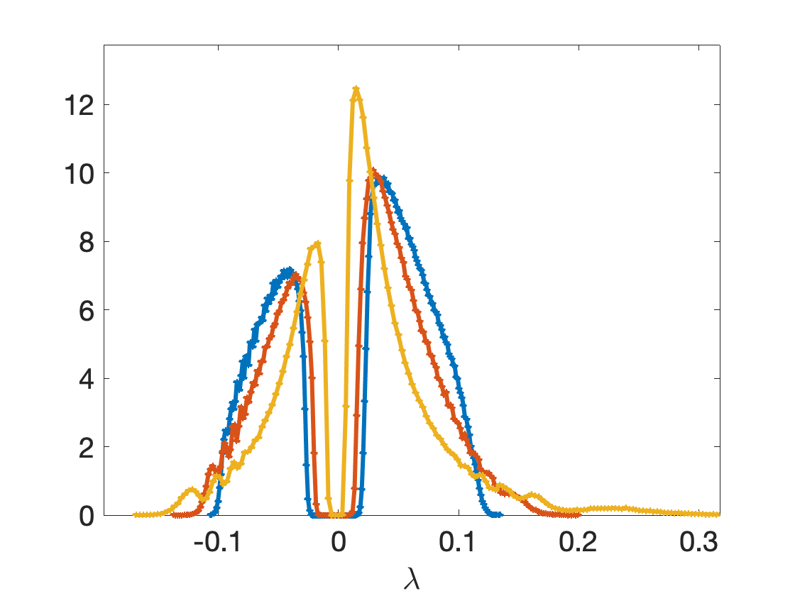
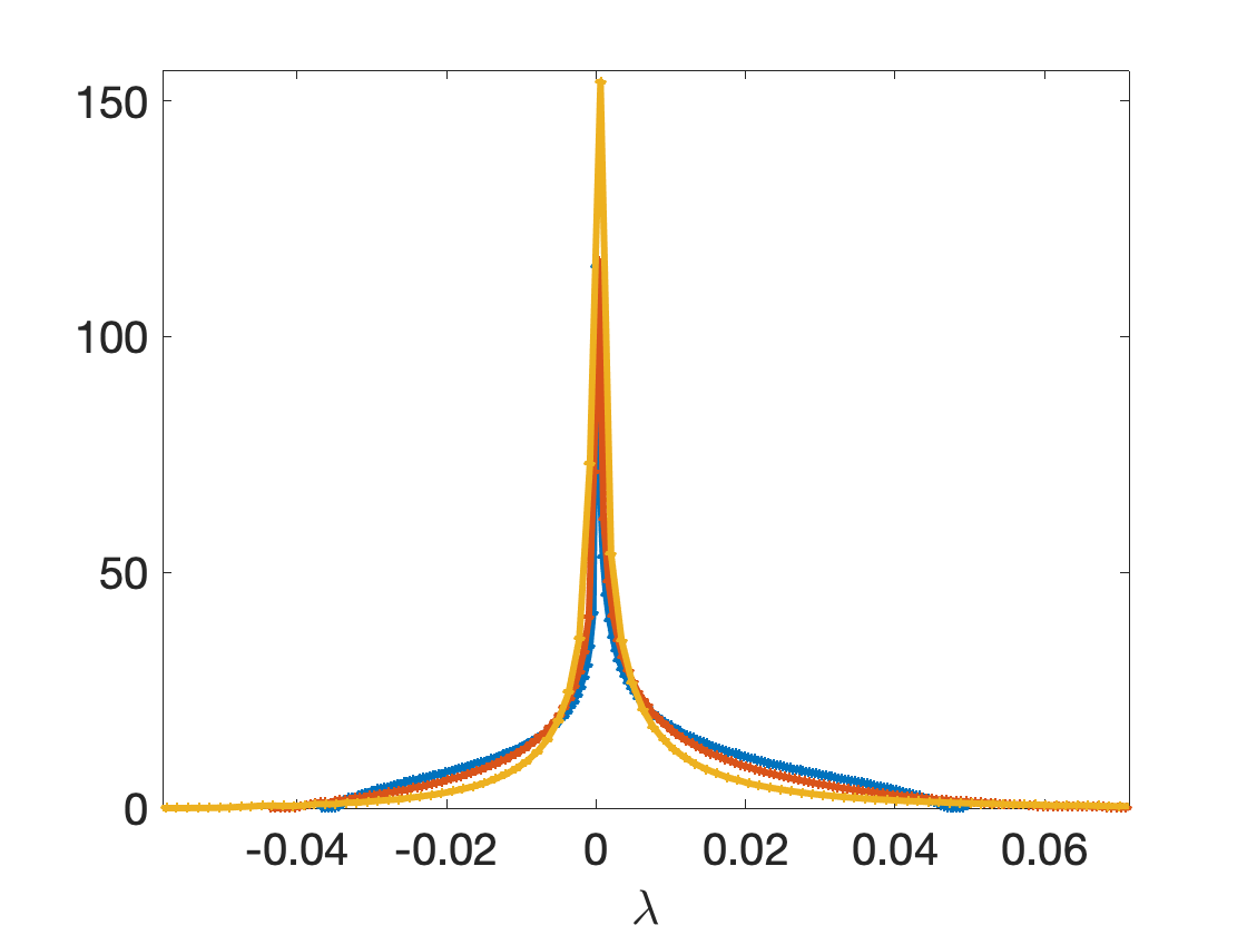
Refer to caption
Refer to caption
Refer to caption
Figure 13: The probability density functions for the negativity spectra at |βϵ0|=0𝛽subscriptitalic-ϵ00|\beta\epsilon_{0}|=0 (blue), 1414\frac{1}{4} (orange), and 1212\frac{1}{2} (yellow). From left to right, we have NB=2subscript𝑁𝐵2N_{B}=2, 444, and 666. The topological transition is robust to finite temperature. We always take NA1=2subscript𝑁subscript𝐴12N_{A_{1}}=2 and NA2=6subscript𝑁subscript𝐴26N_{A_{2}}=6.

5 Implications for mixed-state entanglement and black hole radiation

We now discuss the operational implications of the above results for {{\mathcal{E}}} and I𝐼I. As reviewed in Sec. 2.2, the mutual information gives an upper bound the distillable entanglement

Ed(A1,A2)12I(A1,A2),subscript𝐸𝑑subscript𝐴1subscript𝐴212𝐼subscript𝐴1subscript𝐴2E_{d}(A_{1},A_{2})\leq{{\frac{1}{2}}}I(A_{1},A_{2}), (5.1)

while the logarithmic negativity gives a lower bound on the exact PPT entanglement cost

Ec(ppt,exact)(A1,A2)(A1,A2).superscriptsubscript𝐸𝑐pptexactsubscript𝐴1subscript𝐴2subscript𝐴1subscript𝐴2E_{c}^{\rm(ppt,exact)}(A_{1},A_{2})\geq{{\mathcal{E}}}(A_{1},A_{2})\ . (5.2)

We observed that at a finite temperature, for various choices of ρ(eq)superscript𝜌eq\rho^{(\rm eq)}, there is a region in the entanglement phase diagram where {{\mathcal{E}}} is volume-like while I𝐼I is sub-volume, and hence 12Imuch-greater-than12𝐼{{\mathcal{E}}}\gg\frac{1}{2}I. Our results suggest that such behavior is likely to be generic for all finite temperature chaotic systems. In this part of the phase diagram, we then have

Ec(exact)Ed(exact).much-greater-thansuperscriptsubscript𝐸𝑐exactsuperscriptsubscript𝐸𝑑exactE_{c}^{\rm(exact)}\gg E_{d}^{\rm(exact)}\,. (5.3)

If we further assume that Ec(ppt)superscriptsubscript𝐸𝑐pptE_{c}^{\rm(ppt)} is extensive when Ec(ppt,exact)superscriptsubscript𝐸𝑐pptexactE_{c}^{\rm(ppt,exact)} is extensive, then a stronger statement can be made,

EcEd.much-greater-thansubscript𝐸𝑐subscript𝐸𝑑E_{c}\gg E_{d}\,. (5.4)

This implies that the preparation of the state of A𝐴A from EPR pairs by LOCC operations is highly irreversible, and it has significant bound entanglement.

It is interesting to contrast the results here with those from random states in [50], which can be seen as thermalized states at infinite temperature. In such states, a regime was found where Ecsubscript𝐸𝑐E_{c} is extensive while I𝐼I (and hence Edsubscript𝐸𝑑E_{d}) is sub-extensive. However, this effect took place for a range of subsystem dimensions which all correspond to c=12𝑐12c={{\frac{1}{2}}} in the thermodynamic limit, as opposed to an O(1)𝑂1O(1) range of c𝑐c between some c0subscript𝑐0c_{0} and 1212{{\frac{1}{2}}}, as we find in the finite temperature examples here. The conclusion about Ecsubscript𝐸𝑐E_{c} in [50] was drawn using entanglement of formation as opposed to logarithmic negativity. On calculating {{\mathcal{E}}} in the infinite temperature case in the same regime at c=12𝑐12c={{\frac{1}{2}}}, we do not find that it becomes extensive while I𝐼I is still sub-extensive.

We can ask whether the preparation of the state ρAsubscript𝜌𝐴\rho_{A} by PPT operations, as opposed to LOCC, is also irreversible in this regime. This question cannot be conclusively answered from our results. With the assumption that Ec(ppt)superscriptsubscript𝐸𝑐pptE_{c}^{\rm(ppt)} is extensive when Ec(ppt,exact)superscriptsubscript𝐸𝑐pptexactE_{c}^{\rm(ppt,exact)} is extensive, there are two logical possibilities, both with interesting physical consequences:

  1. 1.

    If Ed(ppt)superscriptsubscript𝐸𝑑pptE_{d}^{\rm(ppt)} is comparable to {{\mathcal{E}}}, i.e. volume-like, as in some known systems [7], then although LOCC distillable entanglement is small, PPT distillable entanglement is large, implying that finite temperature greatly enhances distillable entanglement if we use PPT operations.

  2. 2.

    If Ed(ppt)superscriptsubscript𝐸𝑑pptE_{d}^{\rm(ppt)} is comparable to I𝐼I, i.e. sub-volume-like, then both the PPT and LOCC distillable entanglements are small, and the state is also highly PPT-irreversible.

The results of the previous section apply to generic chaotic many-body systems, and hence also have implications for an evaporating black hole, which is believed to be highly chaotic.

Consider a black hole formed from the collapse of a star initially in a pure state. The black hole subsequently evaporates by emitting Hawking radiation. The evaporation process is very slow in microscopic scales, and we can treat the remaining black hole as well as the radiation as being in macroscopic equilibrium. 171717The two systems can be in separate macroscopic equilibria, because in general the radiation is separated from the black hole after it is emitted. The full system is still in a pure state, and the reduced density operator of each subsystem can be far from the density operators of thermal ensembles. The results of the previous section can be used to predict the entanglement structure within the radiation subsystem, or entanglement between a part of radiation and the remaining black hole, at both infinite and finite temperatures. For definiteness, we will take A𝐴A to be the radiation and B𝐵B to be the black hole.

In [51], from averaging over random pure states, Page found that the entanglement entropy of the radiation undergoes a transition from increasing to decreasing behavior at some time scale t=tp𝑡subscript𝑡𝑝t=t_{p} where logdA=logdBsubscript𝑑𝐴subscript𝑑𝐵\log d_{A}=\log d_{B}. Page’s calculation was in the infinite temperature case, where from our discussion in section 4.2, we know that tpsubscript𝑡𝑝t_{p} is also the time scale at which entanglement within the radiation, as quantified by either I𝐼I or {{\mathcal{E}}}, starts to become extensive. In other words, before the Page time tpsubscript𝑡𝑝t_{p} there is no entanglement within the radiation.

The natural finite-temperature generalization of the Page time is when SA(eq)=SB(eq)superscriptsubscript𝑆𝐴eqsuperscriptsubscript𝑆𝐵eqS_{A}^{(\rm eq)}=S_{B}^{(\rm eq)}, corresponding to c=12𝑐12c={{\frac{1}{2}}}, which was already used in [52]. Our results from the equilibrium approximation and resolvent calculations confirm that this is indeed the time at which the entanglement entropy transitions from increasing to decreasing behavior. Interestingly, our results for logarithmic negativity give a new prediction for the quantum-informational properties of the radiation at finite temperature: there are significant entanglement correlations within the radiation long before the Page time. This suggests the existence of another time scale tbsubscript𝑡𝑏t_{b} when quantum entanglement within the radiation starts becoming extensive. For time scales t(tb,tp)𝑡subscript𝑡𝑏subscript𝑡𝑝t\in(t_{b},t_{p}), the entanglement correlations within the radiation cannot be distilled using LOCC, i.e. they are an example of “bound entanglement.” It is an interesting open question whether this entanglement could be distillable using more general operations such as PPT operations.

Our results from the previous section can also be used to derive replica wormhole contributions to the calculation of the negativity between parts of the radiation in Euclidean gravity. We show these replica wormholes explicitly for the model of [4] in Appendix C.3.1. (See Fig. 26.) Due to specific features of the density of states in JT gravity, the difference between tbsubscript𝑡𝑏t_{b} and tpsubscript𝑡𝑝t_{p} is suppressed in the large quantity S0subscript𝑆0S_{0} in this model. However, this difference should be macroscopically large for higher-dimensional black holes.

To make predictions for the mixed-state entanglement between the black hole and some part of the radiation, we can take A1subscript𝐴1A_{1} and B𝐵B to be parts of the radiation and A2subscript𝐴2A_{2} to be the black hole.

To explore further the nature of entanglement among various parts of the full black hole system, it is instructive to consider the Hayden-Preskill thought experiment at a finite temperature: we throw a diary into the black hole, and see when the information of the diary is recoverable from the radiation. We turn to this problem next. We will find that both time scales tpsubscript𝑡𝑝t_{p} and tbsubscript𝑡𝑏t_{b} can be given operational interpretations in the context of this question.

6 Implications for information transfer from black hole to radiation

In this section, we investigate how information is transferred from the black hole to the radiation during the evaporation process using the Hayden-Preskill thought experiment [10]. Suppose we throw a secret diary D𝐷D into a black hole B𝐵B at an early stage in the evaporation process. As the black hole evaporates, we collect all of the radiation and refer to it as R𝑅R, and refer to the remaining black hole as Bsuperscript𝐵B^{\prime}. Suppose we know the initial state of B𝐵B, and have access to a universal quantum computer with which we can act on the radiation R𝑅R. We then ask how much of the radiation we need in order to learn the initial state of the diary, ρDsubscript𝜌𝐷\rho_{D}.

We can make this question more explicit in the following way. The relevant decompositions of the Hilbert space at the initial and final times respectively are =DBtensor-productsubscript𝐷subscript𝐵{{\mathcal{H}}}={{\mathcal{H}}}_{D}\otimes{{\mathcal{H}}}_{B} and =BRtensor-productsubscriptsuperscript𝐵subscript𝑅{{\mathcal{H}}}={{\mathcal{H}}}_{B^{\prime}}\otimes{{\mathcal{H}}}_{R}. We can consider the following quantum channel from Dsubscript𝐷{{\mathcal{H}}}_{D} to Rsubscript𝑅{{\mathcal{H}}}_{R},

𝒩(ρD)=TrB[U(ρDρB)U],𝒩subscript𝜌𝐷subscriptTrsuperscript𝐵delimited-[]𝑈tensor-productsubscript𝜌𝐷subscript𝜌𝐵superscript𝑈\displaystyle\mathcal{N}(\rho_{D})=\text{Tr}_{B^{\prime}}\left[U\left(\rho_{D}\otimes\rho_{B}\right)U^{\dagger}\right], (6.1)

where U𝑈U is the time-evolution operator for the black hole and radiation, together with the diary, and ρB=|ψ0ψ0|Bsubscript𝜌𝐵ketsubscript𝜓0subscriptbrasubscript𝜓0𝐵\rho_{B}=\ket{\psi_{0}}\bra{\psi_{0}}_{B} is some fixed initial pure state of the black hole. Asking whether we can learn the state of the diary from the radiation is equivalent to asking whether there exists a universal recovery channel {\mathcal{R}} such that 𝒩(ρD)=ρD𝒩subscript𝜌𝐷subscript𝜌𝐷{\mathcal{R}}\circ{{\mathcal{N}}}(\rho_{D})=\rho_{D} for all ρDsubscript𝜌𝐷\rho_{D}.

Note that while we will mostly discuss the above question in terms of evaporating black holes in this section, it can also be seen as a more general question about thermalized states in quantum many-body systems. Suppose we put some information in a small subsystem D𝐷D, and then let D𝐷D evolve together with the rest of the system, B𝐵B. Then given some subsystem R𝑅R in the thermalized state, can we learn the initial state of D𝐷D?

We will take three different approaches to this question, each of which reveals different aspects of the transfer of information from the black hole to the radiation. We will use the equilibrium approximation in each of these approaches, which allows us to understand the transfer of information both at infinite and finite temperature. Note that all statements at finite temperature below are based on the canonical ensemble universality class, where we take α=eβ1HBeβ2HRsubscript𝛼tensor-productsuperscript𝑒subscript𝛽1subscript𝐻superscript𝐵superscript𝑒subscript𝛽2subscript𝐻𝑅{{\mathcal{I}}}_{{\alpha}}=e^{\beta_{1}H_{B^{\prime}}}\otimes e^{\beta_{2}H_{R}}. We will assume that the Hilbert space of the diary has a finite dimension dDsubscript𝑑𝐷d_{D}. We will in general consider the case where the diary can be large, so that dDsubscript𝑑𝐷d_{D} can be O(e1/GN)𝑂superscript𝑒1subscript𝐺𝑁O(e^{1/G_{N}}).

  1. 1.

    We first introduce a reference system Q𝑄Q with the same Hilbert space dimension as D𝐷D, and consider an initial state in which D𝐷D is maximally entangled with Q𝑄Q. The time-evolution on Qsubscript𝑄{{\mathcal{H}}}_{Q} is trivial, while BDtensor-productsubscript𝐵subscript𝐷{{\mathcal{H}}}_{B}\otimes{{\mathcal{H}}}_{D} is evolved with U𝑈U. We then look at the mutual information I(Q,R)𝐼𝑄𝑅I(Q,R) under time-evolution, which can be seen as a way of quantifying the extent to which the radiation contains information about the diary. The behavior of this quantity motivates us to define two natural time-scales:

    • tp1subscript𝑡subscript𝑝1t_{p_{1}}, the time at which SR(eq)=SB(eq)logdDsubscriptsuperscript𝑆eq𝑅subscriptsuperscript𝑆eqsuperscript𝐵subscript𝑑𝐷S^{\rm(eq)}_{R}=S^{\rm(eq)}_{B^{\prime}}-\log d_{D}. I(Q,R)𝐼𝑄𝑅I(Q,R) starts increasing from its initial value of zero at this time.

    • tp2subscript𝑡subscript𝑝2t_{p_{2}}, at which SR(eq)=SB(eq)+logdDsubscriptsuperscript𝑆eq𝑅subscriptsuperscript𝑆eqsuperscript𝐵subscript𝑑𝐷S^{\rm(eq)}_{R}=S^{\rm(eq)}_{B^{\prime}}+\log d_{D}. I(Q,R)𝐼𝑄𝑅I(Q,R) reaches its maximal value of 2logdD2subscript𝑑𝐷2\log d_{D} at this time.

    The standard Page time tpsubscript𝑡𝑝t_{p}, at which we have SR(eq)=SB(eq)superscriptsubscript𝑆𝑅eqsuperscriptsubscript𝑆superscript𝐵eqS_{R}^{\rm(eq)}=S_{B^{\prime}}^{\rm(eq)}, lies between these two time scales.

    When I(Q,R)𝐼𝑄𝑅I(Q,R) reaches its maximal value at tp2subscript𝑡subscript𝑝2t_{p_{2}}, this can be interpreted by saying that all the information that was initially in the diary is now present in the radiation. This statement can be understood operationally in terms of the quantum channel 𝒩𝒩{{\mathcal{N}}} in (6.1). From the results of [53], I(Q,R)=2logdD𝐼𝑄𝑅2subscript𝑑𝐷I(Q,R)=2\log d_{D} implies the existence of a universal recovery channel {\mathcal{R}} for 𝒩𝒩{{\mathcal{N}}}, i.e. 𝒩(ρD)=ρD𝒩subscript𝜌𝐷subscript𝜌𝐷{\mathcal{R}}\circ{{\mathcal{N}}}(\rho_{D})=\rho_{D} for all ρDsubscript𝜌𝐷\rho_{D}. This is consistent with the fact that from a gravitational perspective, tp2subscript𝑡subscript𝑝2t_{p_{2}} is the latest time at which an island can form [2] (see Fig. 14).

  2. 2.

    For some choice of reference state σDsubscript𝜎𝐷\sigma_{D}, and any state ρDsubscript𝜌𝐷\rho_{D}, we compute the difference in the relative entropies before and after applying the channel 𝒩𝒩{{\mathcal{N}}},

    D(𝒩(ρD)||𝒩(σD))D(ρD||σD),D({{\mathcal{N}}}(\rho_{D})||{{\mathcal{N}}}(\sigma_{D}))-D(\rho_{D}||\sigma_{D}), (6.2)

    in order to find a lower bound for the fidelity of some recovery channel {\mathcal{R}} using (2.64). The relevant time scales for this quantity turn out in general to depend on the choice of σDsubscript𝜎𝐷\sigma_{D} and ρDsubscript𝜌𝐷\rho_{D}, and are given by

    • tp(ρD)subscript𝑡𝑝subscript𝜌𝐷t_{p}(\rho_{D}), the time at which SR(eq)=SB(eq)+S(ρD)subscriptsuperscript𝑆eq𝑅subscriptsuperscript𝑆eqsuperscript𝐵𝑆subscript𝜌𝐷S^{\rm(eq)}_{R}=S^{\rm(eq)}_{B^{\prime}}+S(\rho_{D}). The lower bound on the fidelity of some recovery channel {\mathcal{R}} first starts to increase from an exponentially small value at this time.

    • tp2(σD,ρD)subscript𝑡subscript𝑝2subscript𝜎𝐷subscript𝜌𝐷t_{p_{2}}(\sigma_{D},\rho_{D}), at which SR(eq)=SB(eq)+D(ρD||σD)+S(ρD)=SB(eq)Tr[ρDlogσD]S^{\rm(eq)}_{R}=S^{\rm(eq)}_{B^{\prime}}+D(\rho_{D}||\sigma_{D})+S(\rho_{D})=S^{\rm(eq)}_{B^{\prime}}-\text{Tr}[\rho_{D}\log\sigma_{D}]. The lower bound on the fidelity reaches its maximal value of 1 at this time-scale.

    Note that if we take ρDsubscript𝜌𝐷\rho_{D} to be pure, then tp(ρD)=tpsubscript𝑡𝑝subscript𝜌𝐷subscript𝑡𝑝t_{p}(\rho_{D})=t_{p}, the standard Page time. If we take σD=𝟏/dDsubscript𝜎𝐷1subscript𝑑𝐷\sigma_{D}=\mathbf{1}/d_{D}, then tp2(σD,ρD)subscript𝑡subscript𝑝2subscript𝜎𝐷subscript𝜌𝐷t_{p_{2}}(\sigma_{D},\rho_{D}) becomes equal to tp2subscript𝑡subscript𝑝2t_{p_{2}} defined in the previous point independently of ρDsubscript𝜌𝐷\rho_{D}, implying that universal recovery is possible after tp2subscript𝑡subscript𝑝2t_{p_{2}}. Recall that in the previous point, universal recovery at tp2subscript𝑡subscript𝑝2t_{p_{2}} was deduced from the complementary perspective that the mutual information I(Q,R)𝐼𝑄𝑅I(Q,R) becomes maximal at this time.

    The lower bound on the fidelity provides an operational way of seeing the gradual transfer of information from the black hole to the radiation between times tpsubscript𝑡𝑝t_{p} and tp2subscript𝑡subscript𝑝2t_{p_{2}}, as the fidelity increases from its minimal value to one in this range of times. However, this quantity does not seem to have a regime which reflects the growth of I(Q,R)𝐼𝑄𝑅I(Q,R) from time tp1subscript𝑡subscript𝑝1t_{p_{1}} to tpsubscript𝑡𝑝t_{p} which we observed in the previous point.

  3. 3.

    We explicitly calculate the fidelity of the Petz recovery map 𝒫𝒫{{\mathcal{P}}} for 𝒩𝒩{{\mathcal{N}}}, taking the initial state ρDsubscript𝜌𝐷\rho_{D} to be pure to simplify calculations. This reveals the following new time scale, which the lower bound in terms of the relative entropy from the previous point is not sensitive to:

    • tbsubscript𝑡𝑏t_{b}, the time at which S12,R(eq)=S2,B(eq)subscriptsuperscript𝑆eq12𝑅subscriptsuperscript𝑆eq2superscript𝐵S^{\rm(eq)}_{{{\frac{1}{2}}},R}=S^{\rm(eq)}_{2,B^{\prime}}. For a large diary, the fidelity of the Petz map starts growing from its initial value of F(ρD||σD)F(\rho_{D}||\sigma_{D}) at this time. Recall from our discussion in section 4.4.1, that this is also the time scale at which the logarithmic negativity between two parts of the radiation starts to become extensive in the canonical ensemble. 181818At the end of this section, we briefly consider an example with the microcanonical ensemble, taking αsubscript𝛼{{\mathcal{I}}}_{{\alpha}} as in (4.87). For this setup, we find that the fidelity of a large diary starts increasing at a time tr<tpsubscript𝑡𝑟subscript𝑡𝑝t_{r}<t_{p}, which can be either earlier or later than tbsubscript𝑡𝑏t_{b}.

    The time at which the fidelity saturates to unity is tp2subscript𝑡subscript𝑝2t_{p_{2}}, consistent with the conclusions of the two other approaches in the previous points.

Note that at infinite temperature and for small diaries such that logdDSB(eq),SR(eq)much-less-thansubscript𝑑𝐷subscriptsuperscript𝑆eqsuperscript𝐵subscriptsuperscript𝑆eq𝑅\log d_{D}\ll S^{\rm(eq)}_{B^{\prime}},S^{\rm(eq)}_{R}, all the different time scales above coincide, i.e. tp1=tb=tp=tp2subscript𝑡subscript𝑝1subscript𝑡𝑏subscript𝑡𝑝subscript𝑡subscript𝑝2t_{p_{1}}=t_{b}=t_{p}=t_{p_{2}}. More generally, allowing for finite temperature and large diaries, we have tp1tptp2subscript𝑡subscript𝑝1subscript𝑡𝑝subscript𝑡subscript𝑝2t_{p_{1}}\leq t_{p}\leq t_{p_{2}} and tbtptp2subscript𝑡𝑏subscript𝑡𝑝subscript𝑡subscript𝑝2t_{b}\leq t_{p}\leq t_{p_{2}}.

6.1 From the perspective of mutual information

We first discuss the transfer of information from the perspective of the mutual information of the radiation with a reference system Q𝑄Q. This approach was considered at infinite temperature in the original discussion of [10] by using random states, and has been recently generalized to generic chaotic systems at infinite temperature using properties of operator growth [54]. We now provide a generalization to finite temperature using the equilibrium approximation.

We take the initial state of the full system to be

|Ψ0=1dDn=0dD1|nQ|nD|ψ0B.ketsubscriptΨ01subscript𝑑𝐷superscriptsubscript𝑛0subscript𝑑𝐷1tensor-productsubscriptket𝑛𝑄subscriptket𝑛𝐷subscriptketsubscript𝜓0𝐵\displaystyle\ket{\Psi_{0}}=\frac{1}{\sqrt{d_{D}}}\sum_{n=0}^{d_{D}-1}\ket{n}_{Q}\otimes\ket{n}_{D}\otimes\ket{\psi_{0}}_{B}. (6.3)

We will take the time evolution in Q𝑄Q to be trivial, so that the n𝑛n-th Renyi entropy of the time-evolved state in subsystem A𝐴A is given by

𝒵n,A=ηAeA¯|(𝟏𝟏)Qn(UU)DBn|ρ0,e,ρ0=|Ψ0Ψ0|.formulae-sequencesubscript𝒵𝑛𝐴quantum-operator-producttensor-productsubscript𝜂𝐴subscript𝑒¯𝐴tensor-productsubscriptsuperscripttensor-product11𝑛𝑄superscriptsubscripttensor-product𝑈superscript𝑈𝐷𝐵𝑛subscript𝜌0𝑒subscript𝜌0ketsubscriptΨ0brasubscriptΨ0{\mathcal{Z}}_{n,A}=\braket{{\eta}_{A}\otimes e_{\bar{A}}\,}{\,(\mathbf{1}\otimes\mathbf{1})^{n}_{Q}\,\otimes\,(U\otimes U^{\dagger})_{DB}^{n}\,}{\,{\rho_{0}}\,,e},\quad\rho_{0}=\ket{\Psi_{0}}\bra{\Psi_{0}}\,. (6.4)

From the fact that the time-evolution in Q𝑄Q is trivial, we immediately have at all times

Sn,Q=logdD.subscript𝑆𝑛𝑄subscript𝑑𝐷S_{n,Q}=\log d_{D}\,. (6.5)

With the initial state (6.3), (6.4) for A=R𝐴𝑅A=R becomes

𝒵n,R=1dDneBηR|(UU)n|(ρ~0)B𝟏DdD,esubscript𝒵𝑛𝑅1superscriptsubscript𝑑𝐷𝑛quantum-operator-producttensor-productsubscript𝑒superscript𝐵subscript𝜂𝑅superscripttensor-product𝑈superscript𝑈𝑛tensor-productsubscriptsubscript~𝜌0𝐵subscript1𝐷subscript𝑑𝐷𝑒{\mathcal{Z}}_{n,R}=\frac{1}{d_{D}^{n}}\braket{e_{B^{\prime}}\otimes\eta_{R}}{(U\otimes U^{\dagger})^{n}}{(\tilde{\rho}_{0})_{B}\otimes\frac{\mathbf{1}_{D}}{d_{D}},e} (6.6)

where ρ~0=|ψ0ψ0|subscript~𝜌0ketsubscript𝜓0brasubscript𝜓0\tilde{\rho}_{0}=\ket{\psi_{0}}\bra{\psi_{0}}. Note that (6.6) can also be seen as the time-evolution of the entanglement entropy of a mixed state with initial entropy logdDsubscript𝑑𝐷\log d_{D}. We can then use (2.26) to find

Sn,R={Sn,R(eq)Sn,R(eq)<Sn,B(eq)+logdDSn,B(eq)+logdDSn,R(eq)>Sn,B(eq)+logdDsubscript𝑆𝑛𝑅casessuperscriptsubscript𝑆𝑛𝑅eqsuperscriptsubscript𝑆𝑛𝑅eqsuperscriptsubscript𝑆𝑛superscript𝐵eqsubscript𝑑𝐷superscriptsubscript𝑆𝑛superscript𝐵eqsubscript𝑑𝐷superscriptsubscript𝑆𝑛𝑅eqsuperscriptsubscript𝑆𝑛superscript𝐵eqsubscript𝑑𝐷S_{n,R}=\begin{cases}S_{n,R}^{\rm(eq)}&S_{n,R}^{\rm(eq)}<S_{n,B^{\prime}}^{\rm(eq)}+\log d_{D}\\ S_{n,B^{\prime}}^{\rm(eq)}+\log d_{D}&S_{n,R}^{\rm(eq)}>S_{n,B^{\prime}}^{\rm(eq)}+\log d_{D}\end{cases} (6.7)

Since the state on the full system is pure,

𝒵n,QR=𝒵n,B=ηBeR|(UU)n|(ρ~0)B𝟏DdD,e.subscript𝒵𝑛𝑄𝑅subscript𝒵𝑛superscript𝐵quantum-operator-producttensor-productsubscript𝜂superscript𝐵subscript𝑒𝑅superscripttensor-product𝑈superscript𝑈𝑛tensor-productsubscriptsubscript~𝜌0𝐵subscript1𝐷subscript𝑑𝐷𝑒{\mathcal{Z}}_{n,QR}={\mathcal{Z}}_{n,B^{\prime}}=\braket{\eta_{B^{\prime}}\otimes e_{R}}{(U\otimes U^{\dagger})^{n}}{(\tilde{\rho}_{0})_{B}\otimes\frac{\mathbf{1}_{D}}{d_{D}},e}. (6.8)

Again using (2.26), we have

Sn,QR=Sn,B={Sn,R(eq)+logdDSn,R(eq)+logdD<Sn,B(eq)Sn,B(eq)Sn,R(eq)+logdD>Sn,B(eq).subscript𝑆𝑛𝑄𝑅subscript𝑆𝑛superscript𝐵casessuperscriptsubscript𝑆𝑛𝑅eqsubscript𝑑𝐷superscriptsubscript𝑆𝑛𝑅eqsubscript𝑑𝐷superscriptsubscript𝑆𝑛superscript𝐵eqsuperscriptsubscript𝑆𝑛superscript𝐵eqsuperscriptsubscript𝑆𝑛𝑅eqsubscript𝑑𝐷superscriptsubscript𝑆𝑛superscript𝐵eqS_{n,QR}=S_{n,B^{\prime}}=\begin{cases}S_{n,R}^{\rm(eq)}+\log d_{D}&S_{n,R}^{\rm(eq)}+\log d_{D}<S_{n,B^{\prime}}^{\rm(eq)}\\ S_{n,B^{\prime}}^{\rm(eq)}&S_{n,R}^{\rm(eq)}+\log d_{D}>S_{n,B^{\prime}}^{\rm(eq)}\end{cases}. (6.9)

The n𝑛n-th Renyi mutual information between Q𝑄Q and R𝑅R is then given by

In(Q,R)={0Sn,R(eq)<Sn,B(eq)logdDlogdD+Sn,R(eq)Sn,B(eq)Sn,B(eq)logdD<Sn,R(eq)<Sn,B(eq)+logdD2logdDSn,R(eq)>Sn,B(eq)+logdDsubscript𝐼𝑛𝑄𝑅cases0subscriptsuperscript𝑆eq𝑛𝑅subscriptsuperscript𝑆eq𝑛superscript𝐵subscript𝑑𝐷subscript𝑑𝐷superscriptsubscript𝑆𝑛𝑅eqsuperscriptsubscript𝑆𝑛superscript𝐵eqsubscriptsuperscript𝑆eq𝑛superscript𝐵subscript𝑑𝐷subscriptsuperscript𝑆eq𝑛𝑅subscriptsuperscript𝑆eq𝑛superscript𝐵subscript𝑑𝐷2subscript𝑑𝐷subscriptsuperscript𝑆eq𝑛𝑅subscriptsuperscript𝑆eq𝑛superscript𝐵subscript𝑑𝐷I_{n}(Q,R)=\begin{cases}0&S^{\rm(eq)}_{n,R}<S^{\rm(eq)}_{n,B^{\prime}}-\log d_{D}\\ \log d_{D}+S_{n,R}^{\rm(eq)}-S_{n,B^{\prime}}^{\rm(eq)}&S^{\rm(eq)}_{n,B^{\prime}}-\log d_{D}<S^{\rm(eq)}_{n,R}<S^{\rm(eq)}_{n,B^{\prime}}+\log d_{D}\\ 2\log d_{D}&S^{\rm(eq)}_{n,R}>S^{\rm(eq)}_{n,B^{\prime}}+\log d_{D}\end{cases}\, (6.10)

and by analytic continuation,

I(Q,R)={0SR(eq)<SB(eq)logdDlogdD+SR(eq)SB(eq)SB(eq)logdD<SR(eq)<SB(eq)+logdD2logdDSR(eq)>SB(eq)+logdD.𝐼𝑄𝑅cases0subscriptsuperscript𝑆eq𝑅subscriptsuperscript𝑆eqsuperscript𝐵subscript𝑑𝐷subscript𝑑𝐷superscriptsubscript𝑆𝑅eqsuperscriptsubscript𝑆superscript𝐵eqsubscriptsuperscript𝑆eqsuperscript𝐵subscript𝑑𝐷subscriptsuperscript𝑆eq𝑅subscriptsuperscript𝑆eqsuperscript𝐵subscript𝑑𝐷2subscript𝑑𝐷subscriptsuperscript𝑆eq𝑅subscriptsuperscript𝑆eqsuperscript𝐵subscript𝑑𝐷I(Q,R)=\begin{cases}0&S^{\rm(eq)}_{R}<S^{\rm(eq)}_{B^{\prime}}-\log d_{D}\\ \log d_{D}+S_{R}^{\rm(eq)}-S_{B^{\prime}}^{\rm(eq)}&S^{\rm(eq)}_{B^{\prime}}-\log d_{D}<S^{\rm(eq)}_{R}<S^{\rm(eq)}_{B^{\prime}}+\log d_{D}\\ 2\log d_{D}&S^{\rm(eq)}_{R}>S^{\rm(eq)}_{B^{\prime}}+\log d_{D}\end{cases}\,. (6.11)

Note that at all times, I(Q,B)=2logdDI(Q,R)𝐼𝑄superscript𝐵2subscript𝑑𝐷𝐼𝑄𝑅I(Q,B^{\prime})=2\log d_{D}-I(Q,R). From [53], when I(Q,R)=2logdD𝐼𝑄𝑅2subscript𝑑𝐷I(Q,R)=2\log d_{D} and I(Q,B)=0𝐼𝑄superscript𝐵0I(Q,B^{\prime})=0, there exists a recovery channel {\mathcal{R}} satisfying 𝒩(ρD)=ρDtensor-product𝒩subscript𝜌𝐷subscript𝜌𝐷{\mathcal{R}}\otimes{{\mathcal{N}}}(\rho_{D})=\rho_{D} for all ρDsubscript𝜌𝐷\rho_{D} under the channel 𝒩𝒩{{\mathcal{N}}} defined in (6.1). Hence, the universal recovery channel exists after a time scale tp2subscript𝑡subscript𝑝2t_{p_{2}}, at which SR(eq)=SB(eq)+logdDsubscriptsuperscript𝑆eq𝑅subscriptsuperscript𝑆eqsuperscript𝐵subscript𝑑𝐷S^{\rm(eq)}_{R}=S^{\rm(eq)}_{B^{\prime}}+\log d_{D}. This result from the equilibrium approximation is consistent with the expectations from [11] and [2].
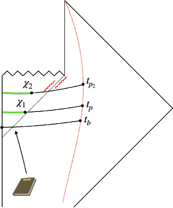
Refer to caption
Figure 14: A Penrose diagram is shown for an evaporating black hole with a large diary thrown into it. We ask when the diary can be reconstructed from the radiation (the fields to the right of the dotted red line). At early times, the entanglement wedge of the radiation is trivial, so the diary cannot be recovered. If the diary was initialized in a pure state, an island (green) forms at tpsubscript𝑡𝑝t_{p} where the nontrivial extremal surface, χ1subscript𝜒1\chi_{1}, becomes smaller than the entropy of the radiation. If the diary was initialized in the maximally mixed state, the island will not form until tp2subscript𝑡subscript𝑝2t_{p_{2}} because the generalized entropy includes the entropy of the diary. While the diary cannot be reconstructed with O(1)𝑂1O(1) fidelity until the island forms, the fidelity exponentially increases from its minimal value starting at the earlier time tbsubscript𝑡𝑏t_{b}.

Note from (6.11) that while the mutual information between the radiation and the auxiliary system becomes maximal at tp2subscript𝑡subscript𝑝2t_{p_{2}}, it begins to grow from zero at an earlier time tp1subscript𝑡subscript𝑝1t_{p_{1}}, at which SR(eq)=SB(eq)logdDsubscriptsuperscript𝑆eq𝑅subscriptsuperscript𝑆eq𝐵subscript𝑑𝐷S^{\rm(eq)}_{R}=S^{\rm(eq)}_{B}-\log d_{D}.

6.2 Recovery channel: bound from relative entropy

We now consider the evolution of the fidelity of recovery channels during the evaporation process. In this subsection, we use (2.64) to put a lower bound on the fidelity of some recovery channel {\mathcal{R}}, by calculating the change of the relative entropy under 𝒩𝒩\mathcal{N} using the equilibrium approximation. In next subsection, we calculate the fidelity of the Petz map explicitly. Note that in both this subsection and the next, we do not include a reference system Q𝑄Q, and the input state for 𝒩𝒩{{\mathcal{N}}} is simply ρDsubscript𝜌𝐷\rho_{D}.

6.2.1 Infinite temperature

For simplicity, let us first consider the infinite temperature case, and take σDsubscript𝜎𝐷\sigma_{D} to be 𝟏D/dDsubscript1𝐷subscript𝑑𝐷\mathbf{1}_{D}/d_{D} and ρDsubscript𝜌𝐷\rho_{D} to be a pure state. Then for the first term in the expression (3.19) for D(𝒩(ρD)||𝒩(σD))D(\mathcal{N}(\rho_{D})||\mathcal{N}(\sigma_{D})), in the infinite temperature case we can sum over all permutations to find (see for instance [1])

Tr[𝒩(ρD)n]=1(dRdB)nτ𝒮ndRk(η1τ)dBk(τ)=dR1nF12(1n,n,2,dRdB)Trdelimited-[]𝒩superscriptsubscript𝜌𝐷𝑛1superscriptsubscript𝑑𝑅subscript𝑑superscript𝐵𝑛subscript𝜏subscript𝒮𝑛superscriptsubscript𝑑𝑅𝑘superscript𝜂1𝜏superscriptsubscript𝑑superscript𝐵𝑘𝜏superscriptsubscript𝑑𝑅1𝑛subscriptsubscript𝐹121𝑛𝑛2subscript𝑑𝑅subscript𝑑superscript𝐵\displaystyle\text{Tr}\left[\mathcal{N}(\rho_{D})^{n}\right]=\frac{1}{(d_{R}d_{B^{\prime}})^{n}}\sum_{\tau\in\mathcal{S}_{n}}d_{R}^{k(\eta^{-1}\tau)}d_{B^{\prime}}^{k(\tau)}=d_{R}^{1-n}{}_{2}F_{1}\left(1-n,-n,2,\frac{d_{R}}{d_{B^{\prime}}}\right) (6.12)

where we consider the regime where dRsubscript𝑑𝑅d_{R} and dBsubscript𝑑superscript𝐵d_{B^{\prime}} are both large, but with no restrictions on the relative sizes. The resulting von Neumann entropy coincides with Page’s formula [51]

S(𝒩(ρD))=limn111nlogTr[𝒩(ρD)n]={logdRdR2dB,dR<dBlogdBdB2dR,dR>dB.𝑆𝒩subscript𝜌𝐷subscript𝑛111𝑛Trdelimited-[]𝒩superscriptsubscript𝜌𝐷𝑛casessubscript𝑑𝑅subscript𝑑𝑅2subscript𝑑superscript𝐵subscript𝑑𝑅subscript𝑑superscript𝐵subscript𝑑superscript𝐵subscript𝑑superscript𝐵2subscript𝑑𝑅subscript𝑑𝑅subscript𝑑superscript𝐵\displaystyle S(\mathcal{N}(\rho_{D}))=\lim_{n\rightarrow 1}\frac{1}{1-n}\log\text{Tr}\left[\mathcal{N}(\rho_{D})^{n}\right]=\begin{cases}\log d_{R}-\frac{d_{R}}{2d_{B^{\prime}}},&d_{R}<d_{B^{\prime}}\\ \log d_{B^{\prime}}-\frac{d_{B^{\prime}}}{2d_{R}},&d_{R}>d_{B^{\prime}}\end{cases}. (6.13)

Using (3.24), the second term in (3.19) is given by a similar sum

Tr[𝒩(ρD)𝒩(σD)n1]=1(dDdRdB)nτSndRk(η1τ)(dDdB)k(τ).Trdelimited-[]𝒩subscript𝜌𝐷𝒩superscriptsubscript𝜎𝐷𝑛11superscriptsubscript𝑑𝐷subscript𝑑𝑅subscript𝑑superscript𝐵𝑛subscript𝜏subscript𝑆𝑛superscriptsubscript𝑑𝑅𝑘superscript𝜂1𝜏superscriptsubscript𝑑𝐷subscript𝑑superscript𝐵𝑘𝜏\displaystyle\text{Tr}\left[\mathcal{N}(\rho_{D})\mathcal{N}(\sigma_{D})^{n-1}\right]=\frac{1}{(d_{D}d_{R}d_{B^{\prime}})^{n}}\sum_{\tau\in S_{n}}d_{R}^{k(\eta^{-1}\tau)}\left(d_{D}d_{B^{\prime}}\right)^{k(\tau)}. (6.14)

This can be interpreted as the entropy of the radiation if it were coupled to an additional bath with a Hilbert space dimension identical to that of the diary. The n1𝑛1n\rightarrow 1 limit is given by

limn111nlogTr[𝒩(ρD)𝒩(σD)n1]={logdRdR2dBdD,dR<dBdDlogdBdDdBdD2dR,dR>dBdD.subscript𝑛111𝑛Trdelimited-[]𝒩subscript𝜌𝐷𝒩superscriptsubscript𝜎𝐷𝑛1casessubscript𝑑𝑅subscript𝑑𝑅2subscript𝑑superscript𝐵subscript𝑑𝐷subscript𝑑𝑅subscript𝑑superscript𝐵subscript𝑑𝐷subscript𝑑superscript𝐵subscript𝑑𝐷subscript𝑑superscript𝐵subscript𝑑𝐷2subscript𝑑𝑅subscript𝑑𝑅subscript𝑑superscript𝐵subscript𝑑𝐷\displaystyle\lim_{n\rightarrow 1}\frac{1}{1-n}\log\text{Tr}\left[\mathcal{N}(\rho_{D})\mathcal{N}(\sigma_{D})^{n-1}\right]=\begin{cases}\log d_{R}-\frac{d_{R}}{2d_{B^{\prime}}d_{D}},&d_{R}<d_{B^{\prime}}d_{D}\\ \log d_{B^{\prime}}d_{D}-\frac{d_{B^{\prime}}d_{D}}{2d_{R}},&d_{R}>d_{B^{\prime}}d_{D}\end{cases}. (6.15)

The relative entropy is therefore

D(𝒩(ρD)||𝒩(σD))\displaystyle D(\mathcal{N}(\rho_{D})||\mathcal{N}(\sigma_{D})) ={dR(dD1)2dBdD,dR<dBlogdRdB+dB2dRdR2dBdD,dB<dR<dBdDlogdD+dB(1dD)2dR,dR>dBdD.absentcasessubscript𝑑𝑅subscript𝑑𝐷12subscript𝑑superscript𝐵subscript𝑑𝐷subscript𝑑𝑅subscript𝑑superscript𝐵subscript𝑑𝑅subscript𝑑superscript𝐵subscript𝑑superscript𝐵2subscript𝑑𝑅subscript𝑑𝑅2subscript𝑑superscript𝐵subscript𝑑𝐷subscript𝑑superscript𝐵subscript𝑑𝑅subscript𝑑superscript𝐵subscript𝑑𝐷subscript𝑑𝐷subscript𝑑superscript𝐵1subscript𝑑𝐷2subscript𝑑𝑅subscript𝑑𝑅subscript𝑑superscript𝐵subscript𝑑𝐷\displaystyle=\begin{cases}\frac{d_{R}(d_{D}-1)}{2d_{B^{\prime}}d_{D}},&d_{R}<d_{B^{\prime}}\\ \log\frac{d_{R}}{d_{B^{\prime}}}+\frac{d_{B^{\prime}}}{2d_{R}}-\frac{d_{R}}{2d_{B^{\prime}}d_{D}},&d_{B^{\prime}}<d_{R}<d_{B^{\prime}}d_{D}\\ \log d_{D}+\frac{d_{B^{\prime}}(1-d_{D})}{2d_{R}},&d_{R}>d_{B^{\prime}}d_{D}\end{cases}. (6.16)

Plugging back into (2.64), we obtain a lower bound on the fidelity:

F(ρ,[σ,𝒩𝒩](ρ)){1dDexp(dR(dD1)2dBdD),dR<dBdRdBdDexp(dB2dRdR2dBdD),dB<dR<dBdDexp(dB(1dD)2dR),dR>dBdD.𝐹𝜌delimited-[]subscript𝜎𝒩𝒩𝜌cases1subscript𝑑𝐷subscript𝑑𝑅subscript𝑑𝐷12subscript𝑑superscript𝐵subscript𝑑𝐷subscript𝑑𝑅subscript𝑑superscript𝐵subscript𝑑𝑅subscript𝑑superscript𝐵subscript𝑑𝐷subscript𝑑superscript𝐵2subscript𝑑𝑅subscript𝑑𝑅2subscript𝑑superscript𝐵subscript𝑑𝐷subscript𝑑superscript𝐵subscript𝑑𝑅subscript𝑑superscript𝐵subscript𝑑𝐷subscript𝑑superscript𝐵1subscript𝑑𝐷2subscript𝑑𝑅subscript𝑑𝑅subscript𝑑superscript𝐵subscript𝑑𝐷\displaystyle F(\rho,[\mathcal{R}_{\sigma,\mathcal{N}}\circ\mathcal{N}](\rho))\geq\begin{cases}\frac{1}{d_{D}}\,{\exp\left({\frac{d_{R}(d_{D}-1)}{2d_{B^{\prime}}d_{D}}}\right)},&d_{R}<d_{B^{\prime}}\\ \frac{d_{R}}{d_{B^{\prime}}d_{D}}\,\exp\left({\frac{d_{B^{\prime}}}{2d_{R}}-\frac{d_{R}}{2d_{B^{\prime}}d_{D}}}\right),&d_{B^{\prime}}<d_{R}<d_{B^{\prime}}d_{D}\\ \exp\left({\frac{d_{B^{\prime}}(1-d_{D})}{2d_{R}}}\right),&d_{R}>d_{B^{\prime}}d_{D}\end{cases}. (6.17)

The transitions between the different lines of (6.17) occur at the infinite-temperature versions of the times tpsubscript𝑡𝑝t_{p} and tp2subscript𝑡subscript𝑝2t_{p_{2}} respectively. The fidelity is exponentially small prior to tpsubscript𝑡𝑝t_{p}. After tpsubscript𝑡𝑝t_{p}, the fidelity is still small but exponentially increases until it reaches a value close to one at tp2subscript𝑡subscript𝑝2t_{p_{2}}. While the formula for exp(D(𝒩(ρD)||𝒩(σD))D(ρD||σD))\exp(D(\mathcal{N}(\rho_{D})||\mathcal{N}(\sigma_{D}))-D(\rho_{D}||\sigma_{D})) on the RHS of (6.17) is only exact in the limit of large Hilbert space dimensions, we find that it is remarkably accurate even for small system sizes in Fig. 15.
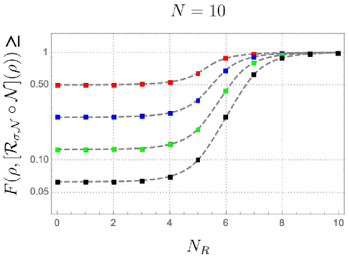
Refer to caption
Figure 15: The lower bound on the fidelity of the Petz map to recover the diary thrown into the black hole from the radiation as a function of the number of qubits NRsubscript𝑁𝑅N_{R} in the radiation, taking the total number of qubits in the system to be N=10𝑁10N=10. The diary is composed of one (red), two (blue), three (green), or four (black) qubits. The dashed lines are the analytic predictions calculated at large N𝑁N, (6.17), although the agreement is already very precise. In the numerical data, we take a fiducial pure state tensored with the diary state and apply a random unitary matrix, computing the relative entropy before and after the random channel. We take 103superscript10310^{3} disorder realizations. Error bars are plotted, though barely visible due to small fluctuations.

6.2.2 Finite temperature

Let us now consider finite temperature, and allow for general choices of the initial state of the diary ρDsubscript𝜌𝐷\rho_{D} and the reference state σDsubscript𝜎𝐷\sigma_{D}. Now, in general, we can no longer perform the sum over all permutations appearing in the equilibrium approximation. We can instead use the formula (3.31) based on the dominant permutations in different regimes, to find191919Note that this formula breaks down and becomes infinite in the large R𝑅R regime if the initial diary states ρDsubscript𝜌𝐷\rho_{D} and σDsubscript𝜎𝐷\sigma_{D} are close to orthogonal. This is guaranteed not to be the case if we choose σDsubscript𝜎𝐷\sigma_{D} to be full rank.

D(𝒩(ρD)||𝒩(σD)){0,SR(eq)<SB(eq)+S(ρD)SR(eq)SB(eq)S(ρD),SB(eq)+S(ρD)<SR(eq)<SB(eq)+D(ρD||σD)+S(ρD)D(ρD||σD),SR(eq)>SB(eq)+D(ρD||σD).\displaystyle D(\mathcal{N}(\rho_{D})||\mathcal{N}(\sigma_{D}))\simeq\begin{cases}0,&S_{R}^{\rm(eq)}<S_{B^{\prime}}^{\rm(eq)}+S(\rho_{D})\\ S_{R}^{\rm(eq)}-S_{B^{\prime}}^{\rm(eq)}-S(\rho_{D}),&S_{B^{\prime}}^{\rm(eq)}+S(\rho_{D})<S_{R}^{\rm(eq)}\\ &<S_{B^{\prime}}^{\rm(eq)}+D(\rho_{D}\lvert\rvert\sigma_{D})+S(\rho_{D})\\ D(\rho_{D}\lvert\rvert\sigma_{D}),&S_{R}^{\rm(eq)}>S_{B^{\prime}}^{\rm(eq)}+D(\rho_{D}\lvert\rvert\sigma_{D})\end{cases}. (6.18)

As an aside, note that we can interpret this result in terms of quantum hypothesis testing, from the standard operational interpretation of the relative entropy. Say Alice were to ask Bob a yes or no question and Bob responded to Alice by writing his answer in his diary (i.e. encoding one of two states ρDsubscript𝜌𝐷\rho_{D} and σDsubscript𝜎𝐷\sigma_{D} in the diary), then throwing it into the black hole, knowing that Alice would collect the radiation from the black hole in order to decode his message using a quantum measurement. If this is repeated over and over, the error rate of Alice misidentifying Bob’s answer is given by eD(𝒩(ρD)||𝒩(σD))e^{-D(\mathcal{N}(\rho_{D})||\mathcal{N}(\sigma_{D}))}.

(6.18) implies the following bound on the fidelity of recovery on using (2.64):

F(ρ,[σ,𝒩𝒩](ρ){eD(ρD||σD),SR(eq)<SB(eq)+S(ρD)eSR(eq)SB(eq)S(ρD)D(ρD||σD),SB(eq)+S(ρD)<SR(eq)<SB(eq)+D(ρD||σD)+S(ρD)1,SR(eq)>SB(eq)+D(ρD||σD)+S(ρD).\displaystyle F(\rho,[\mathcal{R}_{\sigma,\mathcal{N}}\circ\mathcal{N}](\rho)\geq\begin{cases}e^{-D(\rho_{D}\lvert\rvert\sigma_{D})},&S_{R}^{\rm(eq)}<S_{B^{\prime}}^{\rm(eq)}+S(\rho_{D})\\ e^{S_{R}^{\rm(eq)}-S_{B^{\prime}}^{\rm(eq)}-S(\rho_{D})-D(\rho_{D}\lvert\rvert\sigma_{D})},&S_{B^{\prime}}^{\rm(eq)}+S(\rho_{D})<S_{R}^{\rm(eq)}\\ &<S_{B^{\prime}}^{\rm(eq)}+D(\rho_{D}\lvert\rvert\sigma_{D})+S(\rho_{D})\\ 1,&S_{R}^{\rm(eq)}>S_{B^{\prime}}^{\rm(eq)}+D(\rho_{D}\lvert\rvert\sigma_{D})+S(\rho_{D})\end{cases}. (6.19)

We now see that the lower bound on fidelity first starts increasing at a time tp(ρD)subscript𝑡𝑝subscript𝜌𝐷t_{p}(\rho_{D}), at which SR(eq)=SB(eq)+S(ρD)superscriptsubscript𝑆𝑅eqsuperscriptsubscript𝑆superscript𝐵eq𝑆subscript𝜌𝐷S_{R}^{\rm(eq)}=S_{B^{\prime}}^{\rm(eq)}+S(\rho_{D}), and reaches its maximal value at tp2(σD,ρD)subscript𝑡subscript𝑝2subscript𝜎𝐷subscript𝜌𝐷t_{p_{2}}(\sigma_{D},\rho_{D}), at which SR(eq)=SB(eq)+D(ρD||σD)+S(ρD)=SB(eq)Tr[ρDlogσD]S^{\rm(eq)}_{R}=S^{\rm(eq)}_{B^{\prime}}+D(\rho_{D}||\sigma_{D})+S(\rho_{D})=S^{\rm(eq)}_{B^{\prime}}-\text{Tr}[\rho_{D}\log\sigma_{D}].

6.3 Recovery channel: the Petz Map and its fidelity

We progress to explicitly evaluating the fidelity of the Petz recovery map. The quantum channel that we seek to reverse is

𝒩:(D):𝒩subscript𝐷\displaystyle\mathcal{N}:\mathcal{L}(\mathcal{H}_{D}) (R)absentsubscript𝑅\displaystyle\rightarrow\mathcal{L}(\mathcal{H}_{R})
ρDsubscript𝜌𝐷\displaystyle\rho_{D} TrB[U(ρDρB)U],maps-toabsentsubscriptTrsuperscript𝐵delimited-[]superscript𝑈tensor-productsubscript𝜌𝐷subscript𝜌𝐵𝑈\displaystyle\mapsto\text{Tr}_{B^{\prime}}\left[U^{\dagger}\left(\rho_{D}\otimes\rho_{B}\right)U\right], (6.20)

As a reminder, the Petz map is given by

𝒫σ,𝒩:(R):subscript𝒫𝜎𝒩subscript𝑅\displaystyle\mathcal{P}_{\sigma,\mathcal{N}}:\mathcal{L}(\mathcal{H}_{R}) (D)absentsubscript𝐷\displaystyle\rightarrow\mathcal{L}(\mathcal{H}_{D})
X𝑋\displaystyle X σ12𝒩(𝒩(σ)12X𝒩(σ)12)σ12.maps-toabsentsuperscript𝜎12superscript𝒩𝒩superscript𝜎12𝑋𝒩superscript𝜎12superscript𝜎12\displaystyle\mapsto\sigma^{\frac{1}{2}}\mathcal{N}^{\dagger}\left(\mathcal{N}(\sigma)^{-\frac{1}{2}}X\mathcal{N}(\sigma)^{-\frac{1}{2}}\right)\sigma^{\frac{1}{2}}. (6.21)

6.3.1 Infinite temperature

We first study Petz recovery at infinite temperature, again taking ρDsubscript𝜌𝐷\rho_{D} to be pure and σDsubscript𝜎𝐷\sigma_{D} to be maximally mixed. Using the equilibrium approximation for this quantity in (3.34) with α=𝟏subscript𝛼1{{\mathcal{I}}}_{{\alpha}}=\mathbf{1}, we have F(ρ,[𝒫σ,𝒩𝒩](ρ))=limm12Fm𝐹𝜌delimited-[]subscript𝒫𝜎𝒩𝒩𝜌subscript𝑚12subscript𝐹𝑚F(\rho,[\mathcal{P}_{\sigma,\mathcal{N}}\circ\mathcal{N}](\rho))=\lim_{m\rightarrow{{\frac{1}{2}}}}F_{m}, where

Fm=1dD2m+3(dRdB)2m+2τ𝒮2m+2dRk(η1τ)dBk(τ)dDk(τ)+ζ(τ)subscript𝐹𝑚1superscriptsubscript𝑑𝐷2𝑚3superscriptsubscript𝑑𝑅subscript𝑑superscript𝐵2𝑚2subscript𝜏subscript𝒮2𝑚2superscriptsubscript𝑑𝑅𝑘superscript𝜂1𝜏superscriptsubscript𝑑superscript𝐵𝑘𝜏superscriptsubscript𝑑𝐷𝑘𝜏𝜁𝜏\displaystyle F_{m}=\frac{1}{d_{D}^{2m+3}(d_{R}d_{B^{\prime}})^{2m+2}}\sum_{\tau\in\mathcal{S}_{2m+2}}d_{R}^{k(\eta^{-1}\tau)}d_{B^{\prime}}^{k(\tau)}d_{D}^{k(\tau)+\zeta(\tau)} (6.22)

where ζ(τ)𝜁𝜏\zeta(\tau) is zero if the first and (m+2)thsuperscript𝑚2𝑡(m+2)^{th} elements are in different cycles in the permutation τ𝜏\tau, and 1 if they are in the same cycle.

At early times, dBdRmuch-greater-thansubscript𝑑superscript𝐵subscript𝑑𝑅d_{B^{\prime}}\gg d_{R} and the identity element will dominate. The identity has ζ(e)=0𝜁𝑒0\zeta(e)=0, so that

Fm=1dDdR2m+1+O(dB1),F(ρ,[𝒫σ,𝒩𝒩](ρ))=1dD=F(ρD,σD).formulae-sequencesubscript𝐹𝑚1subscript𝑑𝐷superscriptsubscript𝑑𝑅2𝑚1𝑂superscriptsubscript𝑑superscript𝐵1𝐹𝜌delimited-[]subscript𝒫𝜎𝒩𝒩𝜌1subscript𝑑𝐷𝐹subscript𝜌𝐷subscript𝜎𝐷\displaystyle F_{m}=\frac{1}{d_{D}d_{R}^{2m+1}}+O\left(d_{B^{\prime}}^{-1}\right),\quad F(\rho,[\mathcal{P}_{\sigma,\mathcal{N}}\circ\mathcal{N}](\rho))=\frac{1}{d_{D}}=F(\rho_{D},\sigma_{D})\,. (6.23)

At late times,when dRdBdDmuch-greater-thansubscript𝑑𝑅subscript𝑑superscript𝐵subscript𝑑𝐷d_{R}\gg d_{B^{\prime}}d_{D} the cyclic permutation will dominate, which has ζ(η)=1𝜁𝜂1\zeta(\eta)=1, so that

Fm=1(dBdD)2m+1+O(dR1),F(ρ,[𝒫σ,𝒩𝒩](ρ))=1.formulae-sequencesubscript𝐹𝑚1superscriptsubscript𝑑superscript𝐵subscript𝑑𝐷2𝑚1𝑂superscriptsubscript𝑑𝑅1𝐹𝜌delimited-[]subscript𝒫𝜎𝒩𝒩𝜌1\displaystyle F_{m}=\frac{1}{(d_{B^{\prime}}d_{D})^{2m+1}}+O\left(d_{R}^{-1}\right),\quad F(\rho,[\mathcal{P}_{\sigma,\mathcal{N}}\circ\mathcal{N}](\rho))=1\,. (6.24)

To understand how the recovery process improves from (6.23) to (6.24) as the size of the radiation grows, we can perform the full sum in (6.22), as we explain later in this subsection. Before turning to this detailed calculation, we can try to understand relevant time scales by looking at the leading corrections at both early and late times:

  1. 1.

    To find the leading corrections to (6.23), note that the permutations with the next largest value of k(τ)𝑘𝜏k(\tau) after the identity are those with a single transposition, e.g. (12). If it were not for the dDζ(τ)superscriptsubscript𝑑𝐷𝜁𝜏d_{D}^{\zeta(\tau)} term, we would need to sum over all such permutations. However, only the permutation that transposes the first and (m+2)thsuperscript𝑚2𝑡(m+2)^{th} elements has ζ(τ)=1𝜁𝜏1\zeta(\tau)=1. Therefore, this permutation gives the leading correction, and on including it we find

    Fm=1dDdR2m+1+1dDdBdR2m+O(dD2dB1).subscript𝐹𝑚1subscript𝑑𝐷superscriptsubscript𝑑𝑅2𝑚11subscript𝑑𝐷subscript𝑑superscript𝐵superscriptsubscript𝑑𝑅2𝑚𝑂superscriptsubscript𝑑𝐷2superscriptsubscript𝑑superscript𝐵1\displaystyle F_{m}=\frac{1}{d_{D}d_{R}^{2m+1}}+\frac{1}{d_{D}d_{B^{\prime}}d_{R}^{2m}}+O\left(d_{D}^{-2}d_{B^{\prime}}^{-1}\right). (6.25)

    so that we find the leading and next-to-leading order contributions to the fidelity at early times to be

    F(ρ,[𝒫σ,𝒩𝒩](ρ))=1dD+dRdDdB,𝐹𝜌delimited-[]subscript𝒫𝜎𝒩𝒩𝜌1subscript𝑑𝐷subscript𝑑𝑅subscript𝑑𝐷subscript𝑑superscript𝐵\displaystyle F(\rho,[\mathcal{P}_{\sigma,\mathcal{N}}\circ\mathcal{N}](\rho))=\frac{1}{d_{D}}+\frac{d_{R}}{d_{D}d_{B^{\prime}}}, (6.26)

    which grows as more radiation is collected, reflecting the improved recovery. This correction starts to give a contribution comparable to the leading term at time tpsubscript𝑡𝑝t_{p}, which indicates that the fidelity starts to grow from its initial value at tpsubscript𝑡𝑝t_{p}. Note also that this correction has the same scaling as the correction in the lower bound (6.17), but is twice as large.

    When the diary is small, the terms with ζ(τ)=0𝜁𝜏0\zeta(\tau)=0 can also be important. There are (2m+22)1binomial2𝑚221\binom{2m+2}{2}-1 leading terms, so that

    Fm=1dDdR2m+1+1dDdBdR2m+m(3+2m)dD2dBdR2m+O(dB2dD2).subscript𝐹𝑚1subscript𝑑𝐷superscriptsubscript𝑑𝑅2𝑚11subscript𝑑𝐷subscript𝑑superscript𝐵superscriptsubscript𝑑𝑅2𝑚𝑚32𝑚superscriptsubscript𝑑𝐷2subscript𝑑superscript𝐵superscriptsubscript𝑑𝑅2𝑚𝑂superscriptsubscript𝑑superscript𝐵2superscriptsubscript𝑑𝐷2\displaystyle F_{m}=\frac{1}{d_{D}d_{R}^{2m+1}}+\frac{1}{d_{D}d_{B^{\prime}}d_{R}^{2m}}+\frac{m(3+2m)}{d_{D}^{2}d_{B^{\prime}}d_{R}^{2m}}+O(d_{B^{\prime}}^{-2}d_{D}^{-2}). (6.27)

    The replica limit m12𝑚12m\rightarrow-{{\frac{1}{2}}} gives

    F(ρ,[𝒫σ,𝒩𝒩](ρ))=1dD(1+dRdBdRdDdB),𝐹𝜌delimited-[]subscript𝒫𝜎𝒩𝒩𝜌1subscript𝑑𝐷1subscript𝑑𝑅subscript𝑑superscript𝐵subscript𝑑𝑅subscript𝑑𝐷subscript𝑑superscript𝐵\displaystyle F(\rho,[\mathcal{P}_{\sigma,\mathcal{N}}\circ\mathcal{N}](\rho))=\frac{1}{d_{D}}\left(1+\frac{d_{R}}{d_{B^{\prime}}}-\frac{d_{R}}{d_{D}d_{B^{\prime}}}\right), (6.28)
  2. 2.

    To understand the time scale at which the late-time value (6.24) is reached, let us now evaluate the leading correction to (6.24). There are now m(m+1)𝑚𝑚1m(m+1) permutations satisfying both k(η1τ)=2m+1𝑘superscript𝜂1𝜏2𝑚1k(\eta^{-1}\tau)=2m+1 and ζ(τ)=1𝜁𝜏1\zeta(\tau)=1, leading to

    Fm=1(dBdD)2m+1+m(m+1)dR(dBdD)2m+O(dR1dD2m1).subscript𝐹𝑚1superscriptsubscript𝑑superscript𝐵subscript𝑑𝐷2𝑚1𝑚𝑚1subscript𝑑𝑅superscriptsubscript𝑑superscript𝐵subscript𝑑𝐷2𝑚𝑂superscriptsubscript𝑑𝑅1superscriptsubscript𝑑𝐷2𝑚1\displaystyle F_{m}=\frac{1}{(d_{B^{\prime}}d_{D})^{2m+1}}+\frac{m(m+1)}{d_{R}(d_{B^{\prime}}d_{D})^{2m}}+O\left(d_{R}^{-1}d_{D}^{-2m-1}\right). (6.29)

    The leading and next-to-leading contributions to the fidelity at late times are therefore

    F(ρ,[𝒫σ,𝒩𝒩](ρ))=1dBdD4dR+O(dR1dD0).𝐹𝜌delimited-[]subscript𝒫𝜎𝒩𝒩𝜌1subscript𝑑superscript𝐵subscript𝑑𝐷4subscript𝑑𝑅𝑂superscriptsubscript𝑑𝑅1superscriptsubscript𝑑𝐷0\displaystyle F(\rho,[\mathcal{P}_{\sigma,\mathcal{N}}\circ\mathcal{N}](\rho))=1-\frac{d_{B^{\prime}}d_{D}}{4d_{R}}+O\left(d_{R}^{-1}d_{D}^{0}\right). (6.30)

    Note that the correction had to be negative because the fidelity is bounded above by unity. The correction becomes comparable to the leading term at times earlier than tp2subscript𝑡subscript𝑝2t_{p_{2}}. Note also that this correction has the same scaling as, but is half the size of, the lower bound correction in (6.17).

    For small diaries, there are (m+1)2superscript𝑚12(m+1)^{2} other terms which are also important in the correction to the late-time value, and we find

    F(ρ,[𝒫σ,𝒩𝒩](ρ))=1dBdD4dR+dB4dR+O(dR2dD1).𝐹𝜌delimited-[]subscript𝒫𝜎𝒩𝒩𝜌1subscript𝑑superscript𝐵subscript𝑑𝐷4subscript𝑑𝑅subscript𝑑superscript𝐵4subscript𝑑𝑅𝑂superscriptsubscript𝑑𝑅2superscriptsubscript𝑑𝐷1\displaystyle F(\rho,[\mathcal{P}_{\sigma,\mathcal{N}}\circ\mathcal{N}](\rho))=1-\frac{d_{B^{\prime}}d_{D}}{4d_{R}}+\frac{d_{B^{\prime}}}{4d_{R}}+O\left(d_{R}^{-2}d_{D}^{-1}\right). (6.31)

Hence, for the infinite temperature case, (6.26) and (6.30) together give the same predictions for the time scales at which the fidelity of 𝒫𝒫{{\mathcal{P}}} first increases and the time scale at which it saturates, as the predictions based on the lower bound for some recovery channel in (6.17).

Finally, we can also examine the crossover regime of (6.22), where the fidelity becomes O(1)𝑂1O(1). At the time tp2subscript𝑡subscript𝑝2t_{p_{2}}, dR=dBdD:=dsubscript𝑑𝑅subscript𝑑superscript𝐵subscript𝑑𝐷assign𝑑d_{R}=d_{B^{\prime}}d_{D}:=d, so the sum simplifies to

Fm1d4m+4τ𝒮2m+2dk(η1τ)+k(τ)dDζ(τ)1.similar-to-or-equalssubscript𝐹𝑚1superscript𝑑4𝑚4subscript𝜏subscript𝒮2𝑚2superscript𝑑𝑘superscript𝜂1𝜏𝑘𝜏superscriptsubscript𝑑𝐷𝜁𝜏1\displaystyle F_{m}\simeq\frac{1}{d^{4m+4}}\sum_{\tau\in\mathcal{S}_{2m+2}}d^{k(\eta^{-1}\tau)+k(\tau)}d_{D}^{\zeta(\tau)-1}. (6.32)

The exponent is maximized at 2m+42𝑚42m+4 when τ𝜏\tau is a non-crossing permutation that has the first and (m+2)thsuperscript𝑚2𝑡(m+2)^{th} factors in the same cycle. Out of the C2m+2subscript𝐶2𝑚2C_{2m+2} total non-crossing permutations (where Cnsubscript𝐶𝑛C_{n} is the nlimit-from𝑛n-th Catalan number), only Cm+12superscriptsubscript𝐶𝑚12C_{m+1}^{2} have ζ(τ)=1𝜁𝜏1\zeta(\tau)=1, a statement we will soon prove. Therefore,

FmCm+12d2m+1.similar-to-or-equalssubscript𝐹𝑚superscriptsubscript𝐶𝑚12superscript𝑑2𝑚1\displaystyle F_{m}\simeq\frac{C_{m+1}^{2}}{d^{2m+1}}. (6.33)

Taking the m12𝑚12m\rightarrow-\frac{1}{2} limit, we find the fidelity at tp2subscript𝑡subscript𝑝2t_{p_{2}} to have an O(1)𝑂1O(1) value independent of the dimensions,

F(ρ,[𝒫σ,𝒩𝒩](ρ))=649π20.72.𝐹𝜌delimited-[]subscript𝒫𝜎𝒩𝒩𝜌649superscript𝜋2similar-to-or-equals0.72\displaystyle F(\rho,[\mathcal{P}_{\sigma,\mathcal{N}}\circ\mathcal{N}](\rho))=\frac{64}{9\pi^{2}}\simeq 0.72. (6.34)

This fidelity is markedly larger than the lower bound from (6.17), which is e120.61similar-to-or-equalssuperscript𝑒120.61e^{-\frac{1}{2}}\simeq 0.61. Again, for small diaries, we include the subleading non-crossing permutation with ζ(τ)=0𝜁𝜏0\zeta(\tau)=0 to find

F(ρ,[𝒫σ,𝒩𝒩](ρ))=649π2+1649π2dD.𝐹𝜌delimited-[]subscript𝒫𝜎𝒩𝒩𝜌649superscript𝜋21649superscript𝜋2subscript𝑑𝐷\displaystyle F(\rho,[\mathcal{P}_{\sigma,\mathcal{N}}\circ\mathcal{N}](\rho))=\frac{64}{9\pi^{2}}+\frac{1-\frac{64}{9\pi^{2}}}{d_{D}}. (6.35)

We now turn to the full calculation of the fidelity in the planar limit, i.e., we carry out the full sum in (6.22) analytically. Recall that the planar limit corresponds to non-crossing permutations τ𝜏\tau where k(η1τ)+k(τ)=2m+3𝑘superscript𝜂1𝜏𝑘𝜏2𝑚3k(\eta^{-1}\tau)+k(\tau)=2m+3. We claim that the subset of these permutations with ζ(τ)=1𝜁𝜏1\zeta(\tau)=1 and k(η1τ)=p𝑘superscript𝜂1𝜏𝑝k(\eta^{-1}\tau)=p is given by a product of Narayana numbers

NC2m+2,ζ=1,p𝑁subscript𝐶formulae-sequence2𝑚2𝜁1𝑝\displaystyle NC_{2m+2,\zeta=1,p} =p1+p2=pNm+1,p1Nm+1,p2=p1=1pNm+1,p1Nm+1,pp1absentsubscriptsubscript𝑝1subscript𝑝2𝑝subscript𝑁𝑚1subscript𝑝1subscript𝑁𝑚1subscript𝑝2superscriptsubscriptsubscript𝑝11𝑝subscript𝑁𝑚1subscript𝑝1subscript𝑁𝑚1𝑝subscript𝑝1\displaystyle=\sum_{p_{1}+p_{2}=p}N_{m+1,p_{1}}N_{m+1,p_{2}}=\sum_{p_{1}=1}^{p}N_{m+1,p_{1}}N_{m+1,p-p_{1}}
=(m+1p2)(m+1p1)4F3(m1,m,1p,2p;2,mp+3,mp+4;1)m+1.absentbinomial𝑚1𝑝2subscriptbinomial𝑚1𝑝14subscript𝐹3𝑚1𝑚1𝑝2𝑝2𝑚𝑝3𝑚𝑝41𝑚1\displaystyle=\frac{\binom{m+1}{p-2}\binom{m+1}{p-1}\,_{4}F_{3}(-m-1,-m,1-p,2-p;2,m-p+3,m-p+4;1)}{m+1}. (6.36)

We note that the previous statement regarding the square of Catalan numbers above (6.33) is the special case where we sum the above equation from p=2𝑝2p=2 to p=2m+2𝑝2𝑚2p=2m+2.

(6.36) can be proven by considering the elements of the permutation group as a circular lattice of 2m+22𝑚22m+2 points then moving to the dual lattice (see Fig. 16). In the dual lattice, we count the number of non-crossing permutations that factorize into non-crossing permutations of m+1𝑚1m+1 and m+1𝑚1m+1 elements. There is a unique non-crossing permutation of the original lattice corresponding to each one of these permutations, commonly known as the “Kreweras complement.” This is the maximally extended permutation in the dual graph that does not cross the permutation. It is clear that for each factorized permutation in the dual lattice, the Kreweras complement in the original lattice has ζ(τ)=1𝜁𝜏1\zeta(\tau)=1. Indeed, the number of non-crossing permutations in the dual graph with k(τ)=p𝑘𝜏𝑝k(\tau)=p is the same as the number of non-crossing permutations in the original graph with k(η1τ)=p𝑘superscript𝜂1𝜏𝑝k(\eta^{-1}\tau)=p. Using this insight and the prior knowledge of counting the number of non-crossing permutations with a given k(τ)𝑘𝜏k(\tau), we arrive at (6.36).

Refer to caption
Figure 16: A circular lattice of 2m+22𝑚22m+2 elements is shown as black dots. The dual lattice is the red dots. We show an example of a non-crossing permutation on the red lattice that factorizes across the first and m+2𝑚2m+2nd elements of the original lattice. Clearly, the Kreweras complement (shown in black lines) connects the first and m+2𝑚2m+2nd elements such that ζ(τ)=1𝜁𝜏1\zeta(\tau)=1.

We can now find the sum over all permutations with ζ(τ)=1𝜁𝜏1\zeta(\tau)=1 in (6.22), which we call F~msubscript~𝐹𝑚\tilde{F}_{m}:

F~msubscript~𝐹𝑚\displaystyle\tilde{F}_{m} =1(dRdBdD)2m+2p=22m+2NC2m+2,ζ=1,pdRp(dDdB)2m+3pabsent1superscriptsubscript𝑑𝑅subscript𝑑superscript𝐵subscript𝑑𝐷2𝑚2superscriptsubscript𝑝22𝑚2𝑁subscript𝐶formulae-sequence2𝑚2𝜁1𝑝superscriptsubscript𝑑𝑅𝑝superscriptsubscript𝑑𝐷subscript𝑑superscript𝐵2𝑚3𝑝\displaystyle=\frac{1}{(d_{R}d_{B^{\prime}}d_{D})^{2m+2}}\sum_{p=2}^{2m+2}NC_{2m+2,\zeta=1,p}d_{R}^{p}(d_{D}d_{B^{\prime}})^{2m+3-p}
=1dBdD{(dRmF12(m,m1,2,dRdDdB))2,dR<dDdB((dDdB)mF12(m,m1,2,dDdBdR))2,dR>dDdB.absent1subscript𝑑superscript𝐵subscript𝑑𝐷casessuperscriptsuperscriptsubscript𝑑𝑅𝑚subscriptsubscript𝐹12𝑚𝑚12subscript𝑑𝑅subscript𝑑𝐷subscript𝑑superscript𝐵2subscript𝑑𝑅subscript𝑑𝐷subscript𝑑superscript𝐵superscriptsuperscriptsubscript𝑑𝐷subscript𝑑superscript𝐵𝑚subscriptsubscript𝐹12𝑚𝑚12subscript𝑑𝐷subscript𝑑superscript𝐵subscript𝑑𝑅2subscript𝑑𝑅subscript𝑑𝐷subscript𝑑superscript𝐵\displaystyle=\frac{1}{d_{B^{\prime}}d_{D}}\begin{cases}\left(d_{R}^{-m}{}_{2}F_{1}\left(-m,-m-1,2,\frac{d_{R}}{d_{D}d_{B^{\prime}}}\right)\right)^{2},&d_{R}<d_{D}d_{B^{\prime}}\\ \left((d_{D}d_{B^{\prime}})^{-m}{}_{2}F_{1}\left(-m,-m-1,2,\frac{d_{D}d_{B^{\prime}}}{d_{R}}\right)\right)^{2},&d_{R}>d_{D}d_{B^{\prime}}\end{cases}. (6.37)

To enumerate the terms with ζ(τ)=0𝜁𝜏0\zeta(\tau)=0 and k(η1τ)=p𝑘superscript𝜂1𝜏𝑝k(\eta^{-1}\tau)=p, we note that this must simply be the remaining non-crossing permutations of which there are N2m+2,pNC2m+2,ζ=1,psubscript𝑁2𝑚2𝑝𝑁subscript𝐶formulae-sequence2𝑚2𝜁1𝑝N_{2m+2,p}-NC_{2m+2,\zeta=1,p}. We refer to this second contribution to Fmsubscript𝐹𝑚F_{m} as F¯msubscript¯𝐹𝑚\bar{F}_{m}, and immediately find

F¯m={1dDdR2m+1F12(2m1,2m2,2,dRdDdB)F~mdD,dR<dDdB1dD(dDdB)2m+1F12(2m1,2m2,2,dDdBdR)F~mdD,dR>dDdBsubscript¯𝐹𝑚cases1subscript𝑑𝐷superscriptsubscript𝑑𝑅2𝑚1subscriptsubscript𝐹122𝑚12𝑚22subscript𝑑𝑅subscript𝑑𝐷subscript𝑑superscript𝐵subscript~𝐹𝑚subscript𝑑𝐷subscript𝑑𝑅subscript𝑑𝐷subscript𝑑superscript𝐵1subscript𝑑𝐷superscriptsubscript𝑑𝐷subscript𝑑superscript𝐵2𝑚1subscriptsubscript𝐹122𝑚12𝑚22subscript𝑑𝐷subscript𝑑superscript𝐵subscript𝑑𝑅subscript~𝐹𝑚subscript𝑑𝐷subscript𝑑𝑅subscript𝑑𝐷subscript𝑑superscript𝐵\displaystyle\bar{F}_{m}=\begin{cases}\frac{1}{d_{D}d_{R}^{2m+1}}\,{}_{2}F_{1}\left(-2m-1,-2m-2,2,\frac{d_{R}}{d_{D}d_{B^{\prime}}}\right)-\frac{\tilde{F}_{m}}{d_{D}},&d_{R}<d_{D}d_{B^{\prime}}\\ \frac{1}{d_{D}(d_{D}d_{B^{\prime}})^{2m+1}}\,{}_{2}F_{1}\left(-2m-1,-2m-2,2,\frac{d_{D}d_{B^{\prime}}}{d_{R}}\right)-\frac{\tilde{F}_{m}}{d_{D}},&d_{R}>d_{D}d_{B^{\prime}}\end{cases} (6.38)

This expression simplifies in the m12𝑚12m\rightarrow-\frac{1}{2} limit to

F¯12=1dDF~12dDsubscript¯𝐹121subscript𝑑𝐷subscript~𝐹12subscript𝑑𝐷\displaystyle\bar{F}_{-\frac{1}{2}}=\frac{1}{d_{D}}-\frac{\tilde{F}_{-\frac{1}{2}}}{d_{D}} (6.39)

Therefore, the fidelity is

F(ρ,[𝒫σ,𝒩𝒩](ρ))={(11dD)dRdBdDF12(12,12,2,dRdDdB)2+1dDdR<dDdB(11dD)F12(12,12,2,dDdBdR)2+1dDdR>dDdB𝐹𝜌delimited-[]subscript𝒫𝜎𝒩𝒩𝜌cases11subscript𝑑𝐷subscript𝑑𝑅subscript𝑑superscript𝐵subscript𝑑𝐷subscriptsubscript𝐹12superscript12122subscript𝑑𝑅subscript𝑑𝐷subscript𝑑superscript𝐵21subscript𝑑𝐷subscript𝑑𝑅subscript𝑑𝐷subscript𝑑superscript𝐵11subscript𝑑𝐷subscriptsubscript𝐹12superscript12122subscript𝑑𝐷subscript𝑑superscript𝐵subscript𝑑𝑅21subscript𝑑𝐷subscript𝑑𝑅subscript𝑑𝐷subscript𝑑superscript𝐵\displaystyle F(\rho,[\mathcal{P}_{\sigma,\mathcal{N}}\circ\mathcal{N}](\rho))=\begin{cases}(1-\frac{1}{d_{D}})\,\frac{d_{R}}{d_{B^{\prime}}d_{D}}\,{}_{2}F_{1}\left({{\frac{1}{2}}},-{{\frac{1}{2}}},2,\frac{d_{R}}{d_{D}d_{B^{\prime}}}\right)^{2}+\frac{1}{d_{D}}&d_{R}<d_{D}d_{B^{\prime}}\\ (1-\frac{1}{d_{D}})\,{}_{2}F_{1}\left({{\frac{1}{2}}},-{{\frac{1}{2}}},2,\frac{d_{D}d_{B^{\prime}}}{d_{R}}\right)^{2}+\frac{1}{d_{D}}&d_{R}>d_{D}d_{B^{\prime}}\end{cases} (6.40)

This expression is plotted in Fig. 17, where it matches perfectly with numerical tests for finite system sizes.
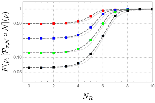
Refer to caption
Figure 17: The fidelity of the Petz map for the Hayden-Preskill protocol at infinite temperature, as a function of the number of qubits NRsubscript𝑁𝑅N_{R} in the radiation. The total number of qubits in the black hole and the radiation is 10 in all cases, and the different curves correspond to different sizes of the diary, ranging from 1 to 4 qubits from top to bottom. The gray dashed curve is the analytic result given by (6.40). The light gray curves are the lower bounds set by the change in relative entropy. In the numerical data, we take a fiducial pure state tensored with the diary state and apply a random unitary matrix and partial trace, followed by the Petz recovery map. We numerically evaluate the between this recovered state and the initial state. Again, we show the average over 103superscript10310^{3} disorder realizations and the corresponding error bars.

6.3.2 Finite temperature

At finite temperature, we have far less control over the contributions from subleading permutations, and hence we are able to find the value of the fidelity corresponding to the sum over all permutations in the equilibrium approximation only in some special cases. First, note that from the general discussion in Section 3.3 based on leading permutations, we expect again that at early times when the identity permutation dominates, the fidelity is given by

F(ρ,[𝒫σ,𝒩𝒩](ρ))=F(ρD,σD).𝐹𝜌delimited-[]subscript𝒫𝜎𝒩𝒩𝜌𝐹subscript𝜌𝐷subscript𝜎𝐷F(\rho,[\mathcal{P}_{\sigma,\mathcal{N}}\circ\mathcal{N}](\rho))=F(\rho_{D},\sigma_{D}). (6.41)

where in the last expression we take σDsubscript𝜎𝐷\sigma_{D} to be an equilibrium density matrix on D𝐷D, and ρDsubscript𝜌𝐷\rho_{D} to be some pure state. Similarly, at sufficiently late times, the cyclic permutation should dominate, so that we have

F(ρ,[𝒫σ,𝒩𝒩](ρ))=1.𝐹𝜌delimited-[]subscript𝒫𝜎𝒩𝒩𝜌1F(\rho,[\mathcal{P}_{\sigma,\mathcal{N}}\circ\mathcal{N}](\rho))=1\,. (6.42)

At intermediate times, the fidelity will interpolate between these values. To probe this regime and find the relevant time scales, let us first look at the leading corrections to the dominant permutations. The first correction to early-time contribution from the identity permutation comes from the permutation that swaps the first and (m+2)thsuperscript𝑚2𝑡(m+2)^{th} copies,

Fmsubscript𝐹𝑚\displaystyle F_{m} =Z2m+2,RZ1,R2m+2F(ρD,σD)+Z2,BZm+1,R2Z1,B2Z1,R2m+2Tr[σD12ρDσD12ρD].absentsubscript𝑍2𝑚2𝑅superscriptsubscript𝑍1𝑅2𝑚2𝐹subscript𝜌𝐷subscript𝜎𝐷subscript𝑍2superscript𝐵superscriptsubscript𝑍𝑚1𝑅2superscriptsubscript𝑍1superscript𝐵2superscriptsubscript𝑍1𝑅2𝑚2Trdelimited-[]superscriptsubscript𝜎𝐷12subscript𝜌𝐷superscriptsubscript𝜎𝐷12subscript𝜌𝐷\displaystyle=\frac{Z_{2m+2,R}}{Z_{1,R}^{2m+2}}F(\rho_{D},\sigma_{D})+\frac{Z_{2,B^{\prime}}Z_{m+1,R}^{2}}{Z_{1,B^{\prime}}^{2}Z_{1,R}^{2m+2}}\text{Tr}\left[\sigma_{D}^{\frac{1}{2}}\rho_{D}\sigma_{D}^{\frac{1}{2}}\rho_{D}\right]. (6.43)

In the replica limit, this can be rewritten in terms of Renyi entropies as

F(ρ,[𝒫σ,𝒩𝒩](ρ))=F(ρD,σD)+eS12,R(eq)S2,B(eq)Tr[σD12ρDσD12ρD].𝐹𝜌delimited-[]subscript𝒫𝜎𝒩𝒩𝜌𝐹subscript𝜌𝐷subscript𝜎𝐷superscript𝑒subscriptsuperscript𝑆eq12𝑅subscriptsuperscript𝑆eq2superscript𝐵Trdelimited-[]superscriptsubscript𝜎𝐷12subscript𝜌𝐷superscriptsubscript𝜎𝐷12subscript𝜌𝐷\displaystyle F(\rho,[\mathcal{P}_{\sigma,\mathcal{N}}\circ\mathcal{N}](\rho))=F(\rho_{D},\sigma_{D})+e^{S^{\rm(eq)}_{\frac{1}{2},R}-S^{\rm(eq)}_{2,B^{\prime}}}\text{Tr}\left[\sigma_{D}^{\frac{1}{2}}\rho_{D}\sigma_{D}^{\frac{1}{2}}\rho_{D}\right]. (6.44)

We can assume Tr[σD12ρDσD12ρD]Trdelimited-[]superscriptsubscript𝜎𝐷12subscript𝜌𝐷superscriptsubscript𝜎𝐷12subscript𝜌𝐷\text{Tr}\left[\sigma_{D}^{\frac{1}{2}}\rho_{D}\sigma_{D}^{\frac{1}{2}}\rho_{D}\right] is of roughly the same magnitude as F(ρD,σD)𝐹subscript𝜌𝐷subscript𝜎𝐷F(\rho_{D},\sigma_{D}) (note that if we take σDsubscript𝜎𝐷\sigma_{D} to be that maximally mixed state and ρDsubscript𝜌𝐷\rho_{D} to be pure, then both are equal to 1dD1subscript𝑑𝐷\frac{1}{d_{D}}). This suggests that the fidelity begins to grow significantly from its initial value at the time scale tbsubscript𝑡𝑏t_{b}, at which S12,R(eq)=S2,B(eq)subscriptsuperscript𝑆eq12𝑅subscriptsuperscript𝑆eq2superscript𝐵S^{\rm(eq)}_{\frac{1}{2},R}=S^{\rm(eq)}_{2,B^{\prime}}.

However, in order to reliably calculate the fidelity past tbsubscript𝑡𝑏t_{b}, we must sum over the contributions from all permutations corresponding to planar diagrams, a calculation we explain in Appendix G.1 using a generating functional method. For this calculation, we assume that σDsubscript𝜎𝐷\sigma_{D} is maximally mixed, ρDsubscript𝜌𝐷\rho_{D} is pure, the radiation is at infinite temperature, and the black hole is at inverse temperature β𝛽\beta, with the density of states as in AdS3𝐴𝑑subscript𝑆3AdS_{3}, ρ(E)=ecVE/V𝜌𝐸superscript𝑒𝑐𝑉𝐸𝑉\rho(E)=e^{cV\sqrt{E/V}}. Now if we define

xlogdRV,ylogdDV,formulae-sequence𝑥subscript𝑑𝑅𝑉𝑦subscript𝑑𝐷𝑉x\equiv{\log d_{R}\over V},\quad y\equiv{\log d_{D}\over V}, (6.45)

where V𝑉V is the volume of Bsuperscript𝐵B^{\prime} and dRsubscript𝑑𝑅d_{R} is the dimension of the radiation, then the various relevant time scales are given by:

tb:x=3c28β,tp:x=c22β,tp2:x=c22β+y.t_{b}:\quad x={3c^{2}\over 8{\beta}},\quad t_{p}:\quad x={c^{2}\over 2{\beta}},\quad t_{p_{2}}:\quad x={c^{2}\over 2{\beta}}+y\ . (6.46)

We find that for small diaries (i.e. y𝑦y is O(V1)𝑂superscript𝑉1O(V^{-1})), the fidelity grows rapidly at tpsubscript𝑡𝑝t_{p} and the time scale tbsubscript𝑡𝑏t_{b} does not turn out to be relevant,

F(ρ,[𝒫σ,𝒩𝒩](ρ)){1dDx<c22β1x>c22β𝐹𝜌delimited-[]subscript𝒫𝜎𝒩𝒩𝜌cases1subscript𝑑𝐷𝑥superscript𝑐22𝛽1𝑥superscript𝑐22𝛽F(\rho,[\mathcal{P}_{\sigma,\mathcal{N}}\circ\mathcal{N}](\rho))\approx\begin{cases}\frac{1}{d_{D}}&x<\frac{c^{2}}{2\beta}\\ 1&x>\frac{c^{2}}{2\beta}\end{cases} (6.47)

with the transition occurring in a region of size O((Vβ)12)𝑂superscript𝑉𝛽12O((V\beta)^{-\frac{1}{2}}) in x𝑥x. On the other hand, for a sufficiently large diary such that there is a regime where 3c28β<x<5c216β+y3superscript𝑐28𝛽𝑥5superscript𝑐216𝛽𝑦\frac{3c^{2}}{8\beta}<x<\frac{5c^{2}}{16\beta}+y, we have

F(ρ,[𝒫σ,𝒩𝒩](ρ))={1dDx<3c28βeV(3c28β+xy)=elogdRS2,BlogdD3c28β<x<5c216β+yeV(cc24β2+xyβx+y)5c216β+y<x<c22β+y1x>c22β+y𝐹𝜌delimited-[]subscript𝒫𝜎𝒩𝒩𝜌cases1subscript𝑑𝐷𝑥3superscript𝑐28𝛽superscript𝑒𝑉3superscript𝑐28𝛽𝑥𝑦superscript𝑒subscript𝑑𝑅subscript𝑆2superscript𝐵subscript𝑑𝐷3superscript𝑐28𝛽𝑥5superscript𝑐216𝛽𝑦superscript𝑒𝑉𝑐superscript𝑐24superscript𝛽2𝑥𝑦𝛽𝑥𝑦5superscript𝑐216𝛽𝑦𝑥superscript𝑐22𝛽𝑦1𝑥superscript𝑐22𝛽𝑦F(\rho,[\mathcal{P}_{\sigma,\mathcal{N}}\circ\mathcal{N}](\rho))=\begin{cases}\frac{1}{d_{D}}&x<\frac{3c^{2}}{8\beta}\\ e^{V(-\frac{3c^{2}}{8\beta}+x-y)}=e^{\log d_{R}-S_{2,B^{\prime}}-\log d_{D}}&\frac{3c^{2}}{8\beta}<x<\frac{5c^{2}}{16\beta}+y\\ e^{V(c\sqrt{-\frac{c^{2}}{4\beta^{2}}+\frac{x-y}{\beta}}-x+y)}&\frac{5c^{2}}{16\beta}+y<x<\frac{c^{2}}{2\beta}+y\\ 1&x>\frac{c^{2}}{2\beta}+y\end{cases} (6.48)

So for a sufficiently large diary, the fidelity starts increasing exponentially from its initial value of 1dD1subscript𝑑𝐷\frac{1}{d_{D}} at time tbsubscript𝑡𝑏t_{b}, and the initial increase is precisely as predicted by (6.44). Note that the lower bound on the fidelity from the change in relative entropy from (6.19) is not sensitive to the time scale tbsubscript𝑡𝑏t_{b}, and only starts growing at the Page time tpsubscript𝑡𝑝t_{p}.

When y𝑦y is O(1)𝑂1O(1) but the diary is not sufficiently large such that such that there is a regime where 3c28β<x<5c216β+y3superscript𝑐28𝛽𝑥5superscript𝑐216𝛽𝑦\frac{3c^{2}}{8\beta}<x<\frac{5c^{2}}{16\beta}+y, the fidelity starts increasing from 1dD1subscript𝑑𝐷\frac{1}{d_{D}} at a time trsubscript𝑡𝑟t_{r} between tbsubscript𝑡𝑏t_{b} and tpsubscript𝑡𝑝t_{p} defined by

tr:x=c22β+2ycyβt_{r}:\quad x=\frac{c^{2}}{2\beta}+2y-c\sqrt{\frac{y}{\beta}} (6.49)

so that we have

F(ρ,[𝒫σ,𝒩𝒩](ρ))={1dDx<c22β+2ycyβeV(cc24β2+xyβx+y)c22β+2ycyβ<x<c22β+y1x>c22β+y𝐹𝜌delimited-[]subscript𝒫𝜎𝒩𝒩𝜌cases1subscript𝑑𝐷𝑥superscript𝑐22𝛽2𝑦𝑐𝑦𝛽superscript𝑒𝑉𝑐superscript𝑐24superscript𝛽2𝑥𝑦𝛽𝑥𝑦superscript𝑐22𝛽2𝑦𝑐𝑦𝛽𝑥superscript𝑐22𝛽𝑦1𝑥superscript𝑐22𝛽𝑦F(\rho,[\mathcal{P}_{\sigma,\mathcal{N}}\circ\mathcal{N}](\rho))=\begin{cases}\frac{1}{d_{D}}&x<\frac{c^{2}}{2\beta}+2y-c\sqrt{\frac{y}{\beta}}\\ e^{V(c\sqrt{-\frac{c^{2}}{4\beta^{2}}+\frac{x-y}{\beta}}-x+y)}&\frac{c^{2}}{2\beta}+2y-c\sqrt{\frac{y}{\beta}}<x<\frac{c^{2}}{2\beta}+y\\ 1&x>\frac{c^{2}}{2\beta}+y\end{cases} (6.50)

trsubscript𝑡𝑟t_{r} is increasingly earlier for larger logdDsubscript𝑑𝐷\log d_{D}, and eventually becomes equal to tbsubscript𝑡𝑏t_{b}.

(6.47),(6.48) and (6.50) are derived with several approximations for the thermodynamic limit. We plot a more exact expression resulting from the calculations of Appendix G.1 for finite but large volumes in Fig. 18. Note in particular that for the case where dDsubscript𝑑𝐷d_{D} is large, we see the initial exponential growth of fidelity eS12,R(eq)S2,B(eq)logdDsuperscript𝑒subscriptsuperscript𝑆eq12𝑅subscriptsuperscript𝑆eq2superscript𝐵subscript𝑑𝐷e^{S^{\rm(eq)}_{{{\frac{1}{2}}},R}-S^{\rm(eq)}_{2,B^{\prime}}-\log d_{D}} predicted by (6.44). For a small diary, the curves obtained from increasing system sizes with fixed logdDsubscript𝑑𝐷\log d_{D} gradually approach an increasingly sharp transition, as expected from (6.47).

The discussion in this section so far has entirely been for the canonical ensemble case. In Appendix G.2, we also consider the example of αsubscript𝛼{{\mathcal{I}}}_{{\alpha}} as in the microcanonical example of (4.87), corresponding to a case where the radiation is divided into two parts R1subscript𝑅1R_{1} and R2subscript𝑅2R_{2} such that there is energy conservation between R1subscript𝑅1R_{1} and Bsuperscript𝐵B^{\prime} while R2subscript𝑅2R_{2} is at infinite temperature. For a small diary, we again find that the fidelity grows from 1dD1subscript𝑑𝐷\frac{1}{d_{D}} to 111 rapidly at tpsubscript𝑡𝑝t_{p}. For a large diary, we find that the fidelity reaches 1 at tp2subscript𝑡subscript𝑝2t_{p_{2}}, and that there is a time scale tr<tpsubscript𝑡𝑟subscript𝑡𝑝t_{r}<t_{p} when the fidelity starts to grow above 1dD1subscript𝑑𝐷\frac{1}{d_{D}}. But for this example, trsubscript𝑡𝑟t_{r} does not seem to be related to the time tbsubscript𝑡𝑏t_{b} at which (R1,R2)subscript𝑅1subscript𝑅2{{\mathcal{E}}}(R_{1},R_{2}) starts to grow in any regime.

Refer to caption
Refer to caption
Figure 18: Left: The fidelity of the Petz recovery map is shown for a diary consisting of a single qubit. The different plots are for different V=100𝑉100V=100, 200200200, 300300300, and 400400400 (from blue to red). The transition approaches the second vertical line, which corresponds to tpsubscript𝑡𝑝t_{p} in the thermodynamic limit. The first vertical line is tbsubscript𝑡𝑏t_{b}. Right: The fidelity of the Petz recovery map for large diaries of sizes 10, 20, 40, and 80 qubits (top to bottom). The first two vertical lines denote tbsubscript𝑡𝑏t_{b} and tpsubscript𝑡𝑝t_{p} which are separated even in the thermodynamic limit. We also display the tp2subscript𝑡subscript𝑝2t_{p_{2}}’s for the respective diary sizes, always with V=100𝑉100V=100. We take R𝑅R to be at infinite temperature and Bsuperscript𝐵B^{\prime} to be at finite temperature with Cardy-like density of states ρ(E)=eVEV𝜌𝐸superscript𝑒𝑉𝐸𝑉\rho(E)=e^{V\sqrt{\frac{E}{V}}} in both plots, taking β=1/2𝛽12\beta=1/2. Notably, the fidelity increases significantly between tbsubscript𝑡𝑏t_{b} and tpsubscript𝑡𝑝t_{p} and does not saturate to one until after tp2subscript𝑡subscript𝑝2t_{p_{2}}.

7 Conclusions and discussions

In this paper, we generalized the equilibrium approximation introduced in [1] to various quantum-informational measures beyond the entanglement entropy, such as Renyi and logarithmic negativities, relative entropy, Petz map fidelity, and reflected entropy. We then studied in detail the entanglement correlations within equilibrated pure states at a finite temperature. We found rich entanglement structures exhibited by the phase diagrams of the logarithmic negativity, mutual information, Renyi negativities, and Renyi mutual informations. In addition to their implications for general quantum chaotic systems, our results also give predictions for the entanglement structure of an evaporating black hole. The verification of these predictions from gravity calculations would help in further probing the quantum nature of black holes as well as informational aspects of quantum gravity. In particular, we predicted the existence of a new time scale tbsubscript𝑡𝑏t_{b} before the Page time, when entanglement correlations within the Hawking radiation start to emerge.

We also studied in detail the process of information recovery from a subsystem, using the Petz map. This issue is central to understanding how and when quantum information is transferred from a black hole to its radiation. We showed that even at finite temperature, the fidelity of the recovery map as well as an upper bound on it provided by relative entropy can be expressed in terms of natural quantum-informational measures in thermal density matrices. Intriguingly, we found evidence that tbsubscript𝑡𝑏t_{b} is the relevant time scale at which the fidelity of recovery starts to increase for a large diary, which suggests that correlations that are detected by negativity but not detected by mutual information play an important role in information recovery.

There are many future directions to explore. Our formulations of the equilibrium approximation for relative entropy and reflected entropy should find other applications. For example, it would be interesting to explore in detail the universal behavior of reflected entropy for finite temperature systems, which we only briefly touched upon. Such studies should also provide further understanding of multipartite entanglement in a quantum many-body system, especially among different parts of the radiation and the black hole.

It would be highly desirable to understand better the nature of the entanglement in the region of the phase diagram where Imuch-greater-than𝐼{{\mathcal{E}}}\gg I. The question is of particular interest for black hole physics. In this regard, it would be interesting to understand whether it is possible to obtain a Lorentzian derivation of the non-zero negativity before the Page time, and see whether there is any semi-classical or geometric description of bound entanglement. Another interesting question is about how new phases which might not correspond to analytic continuation, similar to the ones we found in Fig. 11, would be manifested in a gravity calculation.

From a purely quantum information-theoretic perspective, it would be interesting to investigate if there are deeper direct connections between logarithmic negativity and recoverability of quantum information. In our calculations for the Hayden-Preskill protocol, the known lower bound on the fidelity of recovery from the relative entropy turned out not to be sensitive to the tbsubscript𝑡𝑏t_{b} time scale at which both the Petz map fidelity and the logarithmic negativity start to grow. Our results thus hint that there could be strictly stronger lower bounds on fidelity of recovery if one considered notions related to the partial transpose.

Acknowledgments

We thank Chris Akers, Tom Faulkner, Simon Lin, and Pratik Rath for sharing their manuscripts with us. This work is supported by the Office of High Energy Physics of U.S. Department of Energy under grant Contract Numbers DE-SC0012567 and DE-SC0020360 (MIT contract # 578218).

Appendix A Properties of the permutation group

We can define a notion of distance between elements σ,τ𝜎𝜏\sigma,\tau of the permutation group 𝒮nsubscript𝒮𝑛{\mathcal{S}}_{n} with the Cayley distance,

d(σ,τ)=nk(στ1).𝑑𝜎𝜏𝑛𝑘𝜎superscript𝜏1d(\sigma,\tau)=n-k(\sigma\tau^{-1}). (A.1)

This definition of the distance is consistent with the triangle inequality,

d(σ,τ)+d(τ,ρ)d(σ,ρ).𝑑𝜎𝜏𝑑𝜏𝜌𝑑𝜎𝜌d(\sigma,\tau)+d(\tau,\rho)\geq d(\sigma,\rho). (A.2)

(A.1) and (A.2) can be used to show that

k(ητ1)+k(τ)𝑘𝜂superscript𝜏1𝑘𝜏\displaystyle k(\eta\tau^{-1})+k(\tau) n+1absent𝑛1\displaystyle\leq n+1 (A.3)
k(η1τ1)+k(τ)𝑘superscript𝜂1superscript𝜏1𝑘𝜏\displaystyle k(\eta^{-1}\tau^{-1})+k(\tau) n+1absent𝑛1\displaystyle\leq n+1 (A.4)
k(η1τ)+k(ητ)𝑘superscript𝜂1𝜏𝑘𝜂𝜏\displaystyle k(\eta^{-1}\tau)+k(\eta\tau) {n+2n evenn+1n oddabsentcases𝑛2𝑛 even𝑛1𝑛 odd\displaystyle\leq\begin{cases}n+2&n\text{ even}\\ n+1&n\text{ odd}\end{cases} (A.5)

where we use the fact k(η)=1𝑘𝜂1k(\eta)=1 for all n𝑛n, k(η2)=2𝑘superscript𝜂22k(\eta^{2})=2 for even n𝑛n, and k(η2)=1𝑘superscript𝜂21k(\eta^{2})=1 for odd n𝑛n. We then also have

k(η1τ)+k(ητ)+k(τ)=k(ητ1)+k(τ)2+k(η1τ1)+k(τ)2+k(ητ1)+k(ητ)2{3n2+2n even3n+32n odd𝑘superscript𝜂1𝜏𝑘𝜂𝜏𝑘𝜏𝑘𝜂superscript𝜏1𝑘𝜏2𝑘superscript𝜂1superscript𝜏1𝑘𝜏2𝑘𝜂superscript𝜏1𝑘𝜂𝜏2cases3𝑛22𝑛 even3𝑛32𝑛 odd\begin{gathered}k(\eta^{-1}\tau)+k(\eta\tau)+k(\tau)\\ =\frac{k(\eta\tau^{-1})+k(\tau)}{2}+\frac{k(\eta^{-1}\tau^{-1})+k(\tau)}{2}+\frac{k(\eta\tau^{-1})+k(\eta\tau)}{2}\leq\begin{cases}\frac{3n}{2}+2&n\text{ even}\\ \frac{3n+3}{2}&n\text{ odd}\end{cases}\end{gathered} (A.6)

where the upper bound follows from the inequalities for the individual terms in the second line, and we have used (for instance) that k(ητ)=k(τ1η1)=k(τ1(η1τ1)τ)=k(η1τ1)𝑘𝜂𝜏𝑘superscript𝜏1superscript𝜂1𝑘superscript𝜏1superscript𝜂1superscript𝜏1𝜏𝑘superscript𝜂1superscript𝜏1k(\eta\tau)=k(\tau^{-1}\eta^{-1})=k(\tau^{-1}(\eta^{-1}\tau^{-1})\tau)=k(\eta^{-1}\tau^{-1}). We will now find the set of permutations that saturates (A.6), which is the same as the set that saturates the inequalities for each of the three terms on the LHS of the second line.

First note that the permutations that saturate the inequality for both the first and the second term are in one-to-one correspondence with the non-crossing partitions of n𝑛n elements. Given a non-crossing partition {a11,,am11},{a12,,am22},,{ak,,amkk}subscriptsuperscript𝑎11subscriptsuperscript𝑎1subscript𝑚1subscriptsuperscript𝑎21subscriptsuperscript𝑎2subscript𝑚2superscript𝑎𝑘subscriptsuperscript𝑎𝑘subscript𝑚𝑘\{a^{1}_{1},...,a^{1}_{m_{1}}\},\{a^{2}_{1},...,a^{2}_{m_{2}}\},...,\{a^{k},...,a^{k}_{m_{k}}\}, where the elements of each set are listed in ascending order, the corresponding permutations are given by

τ1=(a11a21am11)(a12am22)(a1kamkk):k(η1τ11)+k(τ1)=n+1\displaystyle\tau_{1}=(a^{1}_{1}~{}a^{1}_{2}...~{}a^{1}_{m_{1}})(a^{2}_{1}~{}...~{}a^{2}_{m_{2}})...(a_{1}^{k}~{}...~{}a^{k}_{m_{k}}):\quad k(\eta^{-1}\tau_{1}^{-1})+k(\tau_{1})=n+1 (A.7)
τ2=(am11a21a11)(am22a12)(amkka1k):k(ητ21)+k(τ2)=n+1\displaystyle\tau_{2}=(a^{1}_{m_{1}}~{}...~{}a^{1}_{2}~{}a^{1}_{1})~{}(a^{2}_{m_{2}}~{}...~{}a^{2}_{1})...(a^{k}_{m_{k}}~{}...~{}a_{1}^{k}):\quad k(\eta\tau_{2}^{-1})+k(\tau_{2})=n+1 (A.8)

The permutations that maximize the sum of the first two terms in the second line of (A.6) are those that lie in the intersection of the above values of τ1subscript𝜏1\tau_{1} and τ2subscript𝜏2\tau_{2}. The difference in the ordering of the elements within the cycles in τ1subscript𝜏1\tau_{1} and τ2subscript𝜏2\tau_{2} does not change the permutation if and only if the permutation consists entirely of one-cycles and two-cycles. Hence, the permutations that simultaneously saturate the inequalities for the first and second terms are in one-to-one correspondence with the non-crossing partitions of n𝑛n elements that have blocks only of size 1 and 2.

Next, note that for any permutation τ𝜏\tau that saturates the inequalities for both the first and the second terms, we have

k(η1τ1)+k(ητ1)=2n+22k(τ)𝑘superscript𝜂1superscript𝜏1𝑘𝜂superscript𝜏12𝑛22𝑘𝜏k(\eta^{-1}\tau^{-1})+k(\eta\tau^{-1})=2n+2-2k(\tau) (A.9)

To maximize the RHS, we need to minimize k(τ)𝑘𝜏k(\tau) among permutations that only have one-cycles and two-cycles.

For even n𝑛n, k(τ)𝑘𝜏k(\tau) is minimized for permutations that only have two cycles, where it is given by n/2𝑛2n/2. Hence, the permutations saturating (A.6) for even n𝑛n are the ones corresponding to non-crossing partitions of n𝑛n elements that have blocks only of size 2. We refer to this set of permutations as {τ}superscript𝜏\{\tau\}^{\ast}. For any such permutation, k(ητ1)=k(ητ)=n2+1𝑘𝜂superscript𝜏1𝑘𝜂𝜏𝑛21k(\eta\tau^{-1})=k(\eta\tau)=\frac{n}{2}+1. The number of such permutations is equal to Cn/2subscript𝐶𝑛2C_{n/2}, where Cn/2subscript𝐶𝑛2C_{n/2} is the Catalan number.

Similarly, for odd n𝑛n, the permutations saturating (A.6) are the ones corresponding to non-crossing partitions of n𝑛n elements that have n12𝑛12\frac{n-1}{2} blocks of size 2 and 1 block of size 1. We refer to this set of permutations as {τ}oddsubscriptsuperscript𝜏odd\{\tau\}^{\ast}_{\rm odd}. For any such permutation, k(τ)=k(ητ1)=k(ητ)=n+12𝑘𝜏𝑘𝜂superscript𝜏1𝑘𝜂𝜏𝑛12k(\tau)=k(\eta\tau^{-1})=k(\eta\tau)=\frac{n+1}{2}. The number of such permutations is equal to nCn12𝑛subscript𝐶𝑛12n~{}C_{\frac{n-1}{2}}.

Refer to caption
Refer to caption
Refer to caption
Figure 19: Boundary conditions for the diagrams corresponding to the three terms in the second line of (A.6).

An alternative way to understand the inequality (A.6) and the permutations that saturate it is in terms of ’tHooft-like double-line diagrams. The first line of (A.6) is equal to the total number of loops in diagrams of the kind shown in Fig. 3, which involve sets of three lines, so we cannot directly modify ’tHooft’s method to that expression. It is useful to separately consider the three terms in the second line of (A.6), each of which can be equated with the total number of loops in a diagram with a different boundary condition. The boundary conditions for the first two terms are as shown in Fig. 19(a) and (b), and the ones for the third term are explained in 19(c), where it will be convenient to use the third form to apply ’tHooft’s method.

By adding an extra loop around each of the diagrams, they can be seen as double-line diagrams, which can then be mapped to polygons by replacing the double lines with single lines. An example of the mapping to polygons for a particular τ𝜏\tau that saturates (A.6), with the boundary conditions of Figs. 19(a) and (c), is shown in Fig. 20. The total number of loops in the double-line diagram is equal to the total number of faces of the corresponding polygon. If the polygon can be flattened on a surface of minimum genus hh, then

F=EV+22h.𝐹𝐸𝑉22F=E-V+2-2h. (A.10)
Refer to caption
Refer to caption
Figure 20: For n=6𝑛6n=6 and τ=(12)(34)(56)𝜏123456\tau=(12)(34)(56), we show the planar double-line diagrams and the corresponding polygons that we get for the first and third terms in the second line of (A.6), using the boundary conditions from (19) (a) and (c).

Now for any given τ𝜏\tau, in the polygons corresponding to the boundary conditions in Fig. 19 (a) and (b), we always have E=3n𝐸3𝑛E=3n and V=2n𝑉2𝑛V=2n, so if for instance F(a)subscript𝐹𝑎F_{(a)} is the number of faces in the diagram for τ𝜏\tau with the boundary conditions of Fig. 19(a) and h(a)subscript𝑎h_{(a)} is the corresponding genus, we have

k(τ)+k(τ1η)=F(a)1=n+12h(a)n+1,k(τ)+k(τ1η1)=F(b)1=n+12h(b)n+1formulae-sequence𝑘𝜏𝑘superscript𝜏1𝜂subscript𝐹𝑎1𝑛12subscript𝑎𝑛1𝑘𝜏𝑘superscript𝜏1superscript𝜂1subscript𝐹𝑏1𝑛12subscript𝑏𝑛1\begin{gathered}k(\tau)+k(\tau^{-1}\eta)=F_{(a)}-1=n+1-2h_{(a)}\leq n+1,\\ k(\tau)+k(\tau^{-1}\eta^{-1})=F_{(b)}-1=n+1-2h_{(b)}\leq n+1\end{gathered} (A.11)

where we subtract 1 from the total number of faces to remove the contribution from the extra line we added around the diagrams. In the polygons corresponding to the boundary conditions in the last figure in 19 (c), we have E=3n1𝐸3𝑛1E=3n-1 and V=2n2𝑉2𝑛2V=2n-2, so

k(ητ1)+k(τη)=F(c)1=n+22h(c)n+2𝑘𝜂superscript𝜏1𝑘𝜏𝜂subscript𝐹𝑐1𝑛22subscript𝑐𝑛2k(\eta\tau^{-1})+k(\tau\eta)=F_{(c)}-1=n+2-2h_{(c)}\leq n+2 (A.12)

Hence, the set of permutations that saturate (A.6) are those that give planar diagrams for each of the Figs. 19 (a), (b) and (c).

Appendix B Estimate of fluctuations in the equilibrium approximation for the negativity

In this appendix, we show that the fluctuations in 𝒵n(PT)superscriptsubscript𝒵𝑛PT{\mathcal{Z}}_{n}^{\rm(PT)} around the equilibrium value, as measured self-consistently by the quantity ΔNsubscriptΔ𝑁\Delta_{N} defined in (3.16), are suppressed relative to the equilibrium value. For this, we need to find the equilibrium approximation for the quantity (𝒵n(PT))2superscriptsuperscriptsubscript𝒵𝑛PT2({\mathcal{Z}}_{n}^{\rm(PT)})^{2}, and compare it to ([𝒵n(PT)]eq approx)2superscriptsubscriptdelimited-[]superscriptsubscript𝒵𝑛PTeq approx2([{\mathcal{Z}}_{n}^{\rm(PT)}]_{\text{eq approx}})^{2}. Let dXsubscript𝑑𝑋d_{X} be the effective Hilbert space dimension of subsystem X𝑋X, and α2:=ηηassignsubscript𝛼2tensor-product𝜂𝜂\alpha_{2}:=\eta\otimes\eta. Then

((𝒵n(PT))2)eq approx=τ2𝒮2neBηA1ηA21|eBηA1ηA21||α,τ2τ2𝒮2ndBk(τ2)dA1k(τ2α21)dA2k(τ2α2)subscriptsuperscriptsuperscriptsubscript𝒵𝑛PT2eq approxsubscriptsubscript𝜏2subscript𝒮2𝑛bratensor-productsubscript𝑒𝐵subscript𝜂subscript𝐴1subscriptsuperscript𝜂1subscript𝐴2bratensor-productsubscript𝑒𝐵subscript𝜂subscript𝐴1subscriptsuperscript𝜂1subscript𝐴2ketsubscript𝛼subscript𝜏2similar-tosubscriptsubscript𝜏2subscript𝒮2𝑛superscriptsubscript𝑑𝐵𝑘subscript𝜏2superscriptsubscript𝑑subscript𝐴1𝑘subscript𝜏2superscriptsubscript𝛼21superscriptsubscript𝑑subscript𝐴2𝑘subscript𝜏2subscript𝛼2\begin{gathered}\left(({\mathcal{Z}}_{n}^{\rm(PT)})^{2}\right)_{~{}\text{eq approx}}=\sum_{\tau_{2}\in{\mathcal{S}}_{2n}}\bra{e_{B}\otimes\eta_{A_{1}}\otimes\eta^{-1}_{A_{2}}}\bra{e_{B}\otimes\eta_{A_{1}}\otimes\eta^{-1}_{A_{2}}}\ket{{{\mathcal{I}}}_{{\alpha}},\tau_{2}}\\ \sim\sum_{\tau_{2}\in{\mathcal{S}}_{2n}}d_{B}^{k(\tau_{2})}d_{A_{1}}^{k(\tau_{2}\alpha_{2}^{-1})}d_{A_{2}}^{k(\tau_{2}\alpha_{2})}\end{gathered} (B.1)

Note that

([𝒵n(PT)]eq approx)2=τ,σ𝒮neBηA1ηA21|eBηA1ηA21||α,τσsuperscriptsubscriptdelimited-[]superscriptsubscript𝒵𝑛PTeq approx2subscript𝜏𝜎subscript𝒮𝑛bratensor-productsubscript𝑒𝐵subscript𝜂subscript𝐴1subscriptsuperscript𝜂1subscript𝐴2bratensor-productsubscript𝑒𝐵subscript𝜂subscript𝐴1subscriptsuperscript𝜂1subscript𝐴2ketsubscript𝛼tensor-product𝜏𝜎([{\mathcal{Z}}_{n}^{\rm(PT)}]_{\text{eq approx}})^{2}=\sum_{\tau,\sigma\in{\mathcal{S}}_{n}}\bra{e_{B}\otimes\eta_{A_{1}}\otimes\eta^{-1}_{A_{2}}}\bra{e_{B}\otimes\eta_{A_{1}}\otimes\eta^{-1}_{A_{2}}}\ket{{{\mathcal{I}}}_{{\alpha}},\tau\otimes\sigma} (B.2)

So

ΔN2=τ2𝒮2n,τ2τσeBηA1ηA21|eBηA1ηA21||α,τ2τ2𝒮2n,τ2τσdBk(τ2)dA1k(τ2α21)dA2k(τ2α2)superscriptsubscriptΔ𝑁2subscriptformulae-sequencesubscript𝜏2subscript𝒮2𝑛subscript𝜏2tensor-product𝜏𝜎bratensor-productsubscript𝑒𝐵subscript𝜂subscript𝐴1subscriptsuperscript𝜂1subscript𝐴2bratensor-productsubscript𝑒𝐵subscript𝜂subscript𝐴1subscriptsuperscript𝜂1subscript𝐴2ketsubscript𝛼subscript𝜏2similar-tosubscriptformulae-sequencesubscript𝜏2subscript𝒮2𝑛subscript𝜏2tensor-product𝜏𝜎superscriptsubscript𝑑𝐵𝑘subscript𝜏2superscriptsubscript𝑑subscript𝐴1𝑘subscript𝜏2superscriptsubscript𝛼21superscriptsubscript𝑑subscript𝐴2𝑘subscript𝜏2subscript𝛼2\begin{gathered}\Delta_{N}^{2}=\sum_{\tau_{2}\in{\mathcal{S}}_{2n},\tau_{2}\neq\tau\otimes\sigma}\bra{e_{B}\otimes\eta_{A_{1}}\otimes\eta^{-1}_{A_{2}}}\bra{e_{B}\otimes\eta_{A_{1}}\otimes\eta^{-1}_{A_{2}}}\ket{{{\mathcal{I}}}_{{\alpha}},\tau_{2}}\\ \sim\sum_{\tau_{2}\in{\mathcal{S}}_{2n},\tau_{2}\neq\tau\otimes\sigma}d_{B}^{k(\tau_{2})}d_{A_{1}}^{k(\tau_{2}\alpha_{2}^{-1})}d_{A_{2}}^{k(\tau_{2}\alpha_{2})}\end{gathered} (B.3)

Let us first consider the entanglement saturation phase, where dA1dA2dBdsimilar-tosubscript𝑑subscript𝐴1subscript𝑑subscript𝐴2similar-tosubscript𝑑𝐵similar-to𝑑d_{A_{1}}\sim d_{A_{2}}\sim d_{B}\sim d. Then

[(𝒵n(PT))2]eq approxτ2𝒮2ndk(τ2)+k(τ2α21)+k(τ2α2)similar-tosubscriptdelimited-[]superscriptsuperscriptsubscript𝒵𝑛PT2eq approxsubscriptsubscript𝜏2subscript𝒮2𝑛superscript𝑑𝑘subscript𝜏2𝑘subscript𝜏2superscriptsubscript𝛼21𝑘subscript𝜏2subscript𝛼2[({\mathcal{Z}}_{n}^{\rm(PT)})^{2}]_{\text{eq approx}}\sim\sum_{\tau_{2}\in{\mathcal{S}}_{2n}}d^{k(\tau_{2})+k(\tau_{2}\alpha_{2}^{-1})+k(\tau_{2}\alpha_{2})} (B.4)

Using the Cayley distance and the triangle inequality for three permutations σ2,τ2,ρ2𝒮2nsubscript𝜎2subscript𝜏2subscript𝜌2subscript𝒮2𝑛\sigma_{2},\tau_{2},\rho_{2}\in{\mathcal{S}}_{2n}, we have

k(σ2τ21)+k(τ2ρ21)2n+k(σ2ρ21)𝑘subscript𝜎2superscriptsubscript𝜏21𝑘subscript𝜏2superscriptsubscript𝜌212𝑛𝑘subscript𝜎2superscriptsubscript𝜌21k(\sigma_{2}\tau_{2}^{-1})+k(\tau_{2}\rho_{2}^{-1})\leq 2n+k(\sigma_{2}\rho_{2}^{-1}) (B.5)

which gives the following upper bound for the exponent in (B.4):

k(τ2)+k(τ2α21)+k(τ2α2)=k(τ21)+k(τ2α21)2+k(α2τ21)+k(τ2α2)2+k(τ21)+k(τ2α2)2{3n+4n even3n+3n odd𝑘subscript𝜏2𝑘subscript𝜏2superscriptsubscript𝛼21𝑘subscript𝜏2subscript𝛼2𝑘superscriptsubscript𝜏21𝑘subscript𝜏2superscriptsubscript𝛼212𝑘subscript𝛼2superscriptsubscript𝜏21𝑘subscript𝜏2subscript𝛼22𝑘superscriptsubscript𝜏21𝑘subscript𝜏2subscript𝛼22cases3𝑛4𝑛 even3𝑛3𝑛 odd\begin{gathered}k(\tau_{2})+k(\tau_{2}\alpha_{2}^{-1})+k(\tau_{2}\alpha_{2})\\ =\frac{k(\tau_{2}^{-1})+k(\tau_{2}\alpha_{2}^{-1})}{2}+\frac{k(\alpha_{2}\tau_{2}^{-1})+k(\tau_{2}\alpha_{2})}{2}+\frac{k(\tau_{2}^{-1})+k(\tau_{2}\alpha_{2})}{2}\leq\begin{cases}3n+4&n\text{ even}\\ 3n+3&n\text{ odd}\end{cases}\end{gathered} (B.6)

We can then check that if τ,σ𝒮n𝜏𝜎subscript𝒮𝑛\tau,\sigma\in{\mathcal{S}}_{n} both saturate (A.6), then τσ𝒮2ntensor-product𝜏𝜎subscript𝒮2𝑛\tau\otimes\sigma\in{\mathcal{S}}_{2n} saturates (B.6). We will now show using ’tHooft-like line diagrams that for any τ2τσsubscript𝜏2tensor-product𝜏𝜎\tau_{2}\neq\tau\otimes\sigma, (B.6) is not saturated. The three terms on the second line of (B.6) can be equated with the total number of loops respectively in the diagrams with boundary conditions shown in Fig. 21 (a), (b) and (c). The leading contribution comes from the permutations that give planar diagrams for each of the three boundary conditions. In particular, any non-factorized permutation gives a non-planar diagram for each of (a), (b) and (c), corresponding to genuses that can be labelled h1,h2,h31subscript1subscript2subscript31h_{1},h_{2},h_{3}\geq 1. With manipulations of the diagrams to the ones used in appendix A, we have

k(τ21)+k(τ2α21)=2n+22h1,k(τ21)+k(τ2α2)=2n+22h2,k(α2τ21)+k(τ2α2)=2n+42h3.formulae-sequence𝑘superscriptsubscript𝜏21𝑘subscript𝜏2superscriptsubscript𝛼212𝑛22subscript1formulae-sequence𝑘superscriptsubscript𝜏21𝑘subscript𝜏2subscript𝛼22𝑛22subscript2𝑘subscript𝛼2superscriptsubscript𝜏21𝑘subscript𝜏2subscript𝛼22𝑛42subscript3\begin{gathered}k(\tau_{2}^{-1})+k(\tau_{2}\alpha_{2}^{-1})=2n+2-2h_{1},\\ k(\tau_{2}^{-1})+k(\tau_{2}\alpha_{2})=2n+2-2h_{2},\\ k(\alpha_{2}\tau_{2}^{-1})+k(\tau_{2}\alpha_{2})=2n+4-2h_{3}.\end{gathered} (B.7)

Hence, all terms contributing to ΔN2superscriptsubscriptΔ𝑁2\Delta_{N}^{2} are of the form

d(2n+22h1)/2+(2n+22h2)/2+(2n+42h3)/2d3n/2+23superscript𝑑2𝑛22subscript122𝑛22subscript222𝑛42subscript32superscript𝑑3𝑛223d^{(2n+2-2h_{1})/2+(2n+2-2h_{2})/2+(2n+4-2h_{3})/2}\leq d^{3n/2+2-3} (B.8)

We therefore find that in the entanglement saturation phase, the fluctuations are suppressed as

ΔN[𝒵n(PT)]eq approxd3/2Z11/2similar-tosubscriptΔ𝑁subscriptdelimited-[]superscriptsubscript𝒵𝑛(PT)eq approxsuperscript𝑑32similar-tosuperscriptsubscript𝑍112\frac{\Delta_{N}}{[{\mathcal{Z}}_{n}^{\text{(PT)}}]_{\text{eq approx}}}\sim d^{-3/2}\sim Z_{1}^{-1/2} (B.9)

where Z1subscript𝑍1Z_{1} is the effect dimension of the full Hilbert space.
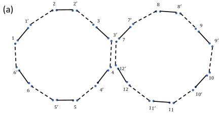
Refer to caption
Refer to caption
Refer to caption
Figure 21: Boundary conditions for the diagrams corresponding to the three terms in the second line of (B.6) are shown in order in (a), (b) and (c).

Next, consider the maximally entangled phase. In this case WLOG, dA1dA2,dBmuch-greater-thansubscript𝑑subscript𝐴1subscript𝑑subscript𝐴2subscript𝑑𝐵d_{A_{1}}\gg d_{A_{2}},d_{B}, so the dominant contribution to [𝒵n(PT)]eq approxsubscriptdelimited-[]superscriptsubscript𝒵𝑛PTeq approx[{\mathcal{Z}}_{n}^{\rm(PT)}]_{\text{eq approx}} comes from τ=η𝜏𝜂\tau=\eta, and the dominant contribution to [(𝒵nPT)2]eq approxsubscriptdelimited-[]superscriptsuperscriptsubscript𝒵𝑛PT2eq approx[({\mathcal{Z}}_{n}^{\rm PT})^{2}]_{\text{eq approx}} comes from τ2=α=ηηsubscript𝜏2𝛼tensor-product𝜂𝜂\tau_{2}=\alpha=\eta\otimes\eta. From any τ2ηηsubscript𝜏2tensor-product𝜂𝜂\tau_{2}\neq\eta\otimes\eta, and in particular any non-factorized τ2subscript𝜏2\tau_{2}, the contribution is suppressed relative to the leading contribution by a factor of at least dA11D1similar-tosuperscriptsubscript𝑑subscript𝐴11superscript𝐷1d_{A_{1}}^{-1}\sim D^{-1}, so

ΔN[𝒵n(PT)]eq approxD1/2similar-tosubscriptΔ𝑁subscriptdelimited-[]superscriptsubscript𝒵𝑛(PT)eq approxsuperscript𝐷12\frac{\Delta_{N}}{[{\mathcal{Z}}_{n}^{\text{(PT)}}]_{\text{eq approx}}}\sim D^{-1/2} (B.10)

Finally, consider the PPT phase. In this case dBdA1,dBmuch-greater-thansubscript𝑑𝐵subscript𝑑subscript𝐴1subscript𝑑𝐵d_{B}\gg d_{A_{1}},d_{B}, so the dominant contribution to [𝒵n(PT)]eq approxsubscriptdelimited-[]superscriptsubscript𝒵𝑛PTeq approx[{\mathcal{Z}}_{n}^{\rm(PT)}]_{\text{eq approx}} comes from τ=e𝜏𝑒\tau=e, and the dominant contribution to [(𝒵n(PT))2]eq approxsubscriptdelimited-[]superscriptsuperscriptsubscript𝒵𝑛PT2eq approx[({\mathcal{Z}}_{n}^{\rm(PT)})^{2}]_{\text{eq approx}} comes from τ2=α=eesubscript𝜏2𝛼tensor-product𝑒𝑒\tau_{2}=\alpha=e\otimes e. Again we have

ΔN[𝒵n(PT)]eq approxD1/2.similar-tosubscriptΔ𝑁subscriptdelimited-[]superscriptsubscript𝒵𝑛(PT)eq approxsuperscript𝐷12\frac{\Delta_{N}}{[{\mathcal{Z}}_{n}^{\text{(PT)}}]_{\text{eq approx}}}\sim D^{-1/2}. (B.11)

Appendix C Resolvent calculations of logarithmic negativity in various cases

C.1 General diagrammatic approach

In order to find the the logarithmic negativity, it is useful to first find the equilibrium approximation for the resolvent

RN(λ)=1λn=01λnTr[(ρAT2)n].subscript𝑅𝑁𝜆1𝜆superscriptsubscript𝑛01superscript𝜆𝑛Trdelimited-[]superscriptsuperscriptsubscript𝜌𝐴subscript𝑇2𝑛R_{N}(\lambda)=\frac{1}{\lambda}\sum_{n=0}^{\infty}\frac{1}{\lambda^{n}}\text{Tr}[(\rho_{A}^{T_{2}})^{n}]\,. (C.1)

It is useful to see RNsubscript𝑅𝑁R_{N} as the trace of a matrix

Rpq=1λn=01λn(ρAT2)npq,|p=|p1A1|p2A2,|q=|q1A1|q2A2formulae-sequencesubscript𝑅𝑝𝑞1𝜆superscriptsubscript𝑛01superscript𝜆𝑛subscriptsuperscriptsuperscriptsubscript𝜌𝐴subscript𝑇2𝑛𝑝𝑞formulae-sequenceket𝑝subscriptketsubscript𝑝1subscript𝐴1subscriptketsubscript𝑝2subscript𝐴2ket𝑞subscriptketsubscript𝑞1subscript𝐴1subscriptketsubscript𝑞2subscript𝐴2R_{pq}=\frac{1}{\lambda}\sum_{n=0}^{\infty}\frac{1}{\lambda^{n}}{(\rho_{A}^{T_{2}})^{n}}_{pq},\quad\ket{p}=\ket{p_{1}}_{A_{1}}\ket{p_{2}}_{A_{2}},\quad\ket{q}=\ket{q_{1}}_{A_{1}}\ket{q_{2}}_{A_{2}} (C.2)

We can apply the equilibrium approximation to each (ρAT2)npqsubscriptsuperscriptsuperscriptsubscript𝜌𝐴subscript𝑇2𝑛𝑝𝑞{(\rho_{A}^{T_{2}})^{n}}_{pq}. The common lower half of the diagrams for all permutations in this case can be deduced from Fig. 3 (a) for Tr[(ρAT2)n]Trdelimited-[]superscriptsuperscriptsubscript𝜌𝐴subscript𝑇2𝑛\text{Tr}[(\rho_{A}^{T_{2}})^{n}] by erasing the dashed line connecting iansubscriptsuperscript𝑖subscript𝑎𝑛i^{\prime}_{a_{n}} and ia1subscript𝑖subscript𝑎1i_{a_{1}}, and the dotted line connecting ia¯1subscriptsuperscript𝑖subscript¯𝑎1i^{\prime}_{\bar{a}_{1}} and ia¯nsubscript𝑖subscript¯𝑎𝑛i_{\bar{a}_{n}}, and instead taking the inner product of |ia1ketsubscript𝑖subscript𝑎1\ket{i_{a_{1}}}, |ia¯1ketsubscriptsuperscript𝑖subscript¯𝑎1\ket{i^{\prime}_{\bar{a}_{1}}}, |ianketsubscript𝑖subscript𝑎𝑛\ket{i_{a_{n}}}, |ia¯nketsubscriptsuperscript𝑖subscript¯𝑎𝑛\ket{i^{\prime}_{\bar{a}_{n}}} with |p1ketsubscript𝑝1\ket{p_{1}}, |p2ketsubscript𝑝2\ket{p_{2}}, |q1ketsubscript𝑞1\ket{q_{1}}, |q2ketsubscript𝑞2\ket{q_{2}} respectively. The resulting lines are shown in Fig. 22, which also explains how the factors of 1λn+11superscript𝜆𝑛1\frac{1}{\lambda^{n+1}} and 1Z1n1superscriptsubscript𝑍1𝑛\frac{1}{Z_{1}^{n}} that are common to all terms with index n𝑛n in (C.1) (the second factor comes from the equilibrium approximation) are incorporated into these lines.

Refer to caption
Figure 22: “Boundary” lines for the equilibrium approximation for Rpqsubscript𝑅𝑝𝑞R_{pq} with n=4𝑛4n=4.

In the limit where the effective dimension of A1subscript𝐴1A_{1} is much larger than that of A2subscript𝐴2A_{2}, it is sufficient to consider contributions from planar diagrams for all n𝑛n to Rpqsubscript𝑅𝑝𝑞R_{pq}. We can write Rpqsubscript𝑅𝑝𝑞R_{pq} in terms of a self-energy ΣpqsubscriptΣ𝑝𝑞\Sigma_{pq} as shown in Fig. 23(a). ΣpqsubscriptΣ𝑝𝑞\Sigma_{pq} is a sum of diagrams without any disconnected parts connected by 1λδpq1𝜆subscript𝛿𝑝𝑞\frac{1}{\lambda}\delta_{pq}, to which the first few contributions are shown in Fig. 23(b). We take |p1,|q1ketsubscript𝑝1ketsubscript𝑞1\ket{p_{1}},\ket{q_{1}} and |p2,|q2ketsubscript𝑝2ketsubscript𝑞2\ket{p_{2}},\ket{q_{2}} to be elements of the energy eigenbasis in A1subscript𝐴1A_{1} and A2subscript𝐴2A_{2} respectively, so that we approximately have that

p1|p2|α|q1|q2δp1q1δp2q2proportional-tobrasubscript𝑝1brasubscript𝑝2subscript𝛼ketsubscript𝑞1ketsubscript𝑞2subscript𝛿subscript𝑝1subscript𝑞1subscript𝛿subscript𝑝2subscript𝑞2\bra{p_{1}}\bra{p_{2}}{{\mathcal{I}}}_{{\alpha}}\ket{q_{1}}\ket{q_{2}}\propto\delta_{p_{1}\,q_{1}}\,\delta_{p_{2}\,q_{2}} (C.3)

for both the canonical and microcanonical ensembles, and hence from the diagrams contributing to ΣpqsubscriptΣ𝑝𝑞\Sigma_{pq} we can see that both ΣpqsubscriptΣ𝑝𝑞\Sigma_{pq} and Rpqsubscript𝑅𝑝𝑞R_{pq} are proportional to δpqsubscript𝛿𝑝𝑞\delta_{pq}.

Refer to caption
Refer to caption
Figure 23: Diagrammatic representation of Rpqsubscript𝑅𝑝𝑞R_{pq} and the first few diagrams contributing to ΣpqsubscriptΣ𝑝𝑞\Sigma_{pq} in the case where A1subscript𝐴1A_{1} is larger than A2subscript𝐴2A_{2}.

We can immediately see by summing the geometric series on the RHS of Fig. 23(a) that

RN=pRp,Rp=1λΣp.formulae-sequencesubscript𝑅𝑁subscript𝑝subscript𝑅𝑝subscript𝑅𝑝1𝜆subscriptΣ𝑝R_{N}=\sum_{p}R_{p},\quad R_{p}=\frac{1}{\lambda-\Sigma_{p}}\,. (C.4)

We can systematically include all planar contributions to ΣpsubscriptΣ𝑝\Sigma_{p} using the Schwinger-Dyson equation shown diagrammatically in Fig. 24. For general choices of αsubscript𝛼{{\mathcal{I}}}_{{\alpha}}, this Schwinger-Dyson equation in general leads to a complicated set of equations relating Rpsubscript𝑅𝑝R_{p} for all different p𝑝p to each other. Below we consider a few choices of αsubscript𝛼{{\mathcal{I}}}_{{\alpha}} for which the Schwinger-Dyson equation simplifies.
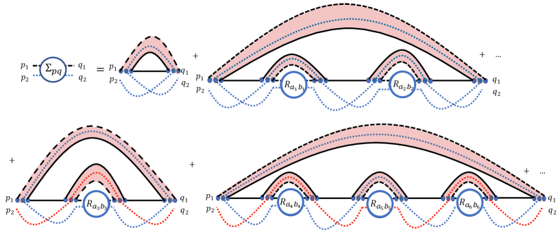
Refer to caption
Figure 24: Rewriting of the RHS of Fig. 23(b) as a Schwinger-Dyson equation. All ai,bisubscript𝑎𝑖subscript𝑏𝑖a_{i},b_{i} are independently summed over (unless they have delta functions among each other or with p,q𝑝𝑞p,q according to the diagram).

C.2 Infinite temperature

We first consider the case where the effective identity operator is simply the identity,

α=𝟏A1𝟏A2𝟏B.subscript𝛼tensor-productsubscript1subscript𝐴1subscript1subscript𝐴2subscript1𝐵{{\mathcal{I}}}_{{\alpha}}=\mathbf{1}_{A_{1}}\otimes\mathbf{1}_{A_{2}}\otimes\mathbf{1}_{B}\,. (C.5)

Here the Schwinger-Dyson equation for Rpsubscript𝑅𝑝R_{p} becomes independent of the index p𝑝p in A𝐴A, and we have

RN=dAR1,R1=1λΣ1.formulae-sequencesuperscriptsubscript𝑅𝑁subscript𝑑𝐴subscript𝑅1subscript𝑅11𝜆subscriptΣ1R_{N}^{\infty}=d_{A}R_{1},\quad R_{1}=\frac{1}{\lambda-\Sigma_{1}}\,. (C.6)

Each line on the RHS of Fig. 24 now simplifies to a geometric series, and hence

Σ1=(1dA+αR1)(1+R12β+(R12β)2+)=(1dA+αR1)11R12β,α=1dAdB,β=1(dA2dB)2\begin{gathered}\Sigma_{1}=\left(\frac{1}{d_{A}}+\alpha R_{1}\right)\,\left(1+R_{1}^{2}\beta+(R_{1}^{2}\beta)^{2}+...\right)=\left(\frac{1}{d_{A}}+\alpha R_{1}\right)\,\frac{1}{1-R_{1}^{2}\beta},\\ \alpha=\frac{1}{d_{A}d_{B}},\quad\beta=\frac{1}{(d_{A_{2}}d_{B})^{2}}\end{gathered} (C.7)

Substituting this into (C.6), we get a cubic equation for R1subscript𝑅1R_{1},

βλR13+(αβ)R12+(1dAλ)R1+1=0.𝛽𝜆superscriptsubscript𝑅13𝛼𝛽superscriptsubscript𝑅121subscript𝑑𝐴𝜆subscript𝑅110\beta\lambda R_{1}^{3}+(\alpha-\beta)R_{1}^{2}+\left(\frac{1}{d_{A}}-\lambda\right)R_{1}+1=0\,. (C.8)

It is difficult to obtain a general analytic expression for 𝒵(PT):=i|λi|=eassignsuperscript𝒵PTsubscript𝑖subscript𝜆𝑖superscript𝑒{\mathcal{Z}}^{\rm(PT)}:=\sum_{i}|\lambda_{i}|=e^{{{\mathcal{E}}}} by finding the analytic form of DN(λ)subscript𝐷𝑁𝜆D_{N}(\lambda) from the solutions to (C.8). However, the density and the logarithmic negativity can be found numerically from (C.8), and turn out to agree with the analytic continuation in (4.17), (4.14), (4.21), as discussed in [9]. That is, we have

𝒵(PT)(dA1,dA2,dB)={1logdA<logdBdA1log(dA1dB)<logdA2dA2log(dA2dB)<logdA1(dAdB)1/2logdA>logdB,|logdA1logdA2|<logdB.subscriptsuperscript𝒵PTsubscript𝑑subscript𝐴1subscript𝑑subscript𝐴2subscript𝑑𝐵cases1subscript𝑑𝐴subscript𝑑𝐵subscript𝑑subscript𝐴1subscript𝑑subscript𝐴1subscript𝑑𝐵subscript𝑑subscript𝐴2subscript𝑑subscript𝐴2subscript𝑑subscript𝐴2subscript𝑑𝐵subscript𝑑subscript𝐴1superscriptsubscript𝑑𝐴subscript𝑑𝐵12formulae-sequencesubscript𝑑𝐴subscript𝑑𝐵subscript𝑑subscript𝐴1subscript𝑑subscript𝐴2subscript𝑑𝐵{\mathcal{Z}}^{\rm(PT)}_{\infty}(d_{A_{1}},d_{A_{2}},d_{B})=\begin{cases}1&\log d_{A}<\log d_{B}\\ d_{A_{1}}&\log{(d_{A_{1}}d_{B})}<\log d_{A_{2}}\\ d_{A_{2}}&\log(d_{A_{2}}d_{B})<\log d_{A_{1}}\\ \left(\frac{d_{A}}{d_{B}}\right)^{1/2}&\log d_{A}>\log d_{B},~{}~{}|\log{d_{A_{1}}}-\log d_{A_{2}}|<\log d_{B}\end{cases}\,. (C.9)

Now consider the regime where dA1dA2dB1much-less-thansubscript𝑑subscript𝐴1subscript𝑑subscript𝐴2subscript𝑑𝐵1\frac{d_{A_{1}}}{d_{A_{2}}d_{B}}\ll 1. This corresponds to being outside the ME phase. Then since αβmuch-greater-than𝛼𝛽\alpha\gg\beta in this regime, R1subscript𝑅1R_{1} is O(1)𝑂1O(1), and λ𝜆\lambda is O(1/dA)𝑂1subscript𝑑𝐴O(1/d_{A}), (C.8) simplifies to a quadratic equation for R1subscript𝑅1R_{1},

αR12+(1dAλ)R1+1=0.𝛼superscriptsubscript𝑅121subscript𝑑𝐴𝜆subscript𝑅110\alpha\,R_{1}^{2}+\left(\frac{1}{d_{A}}-\lambda\right)R_{1}+1=0. (C.10)

The same quadratic equation can be obtained diagrammatically by ignoring all contributions to the Schwinger-Dyson equation in Fig. 24 except the first term in each line on the RHS. This corresponds to including contributions from permutations with only one-cycles and two-cycles to 𝒵n(PT)superscriptsubscript𝒵𝑛PT{\mathcal{Z}}_{n}^{\rm(PT)} for all n𝑛n. We can now solve (C.10) to get a simple semicircle form of DN(λ)subscript𝐷𝑁𝜆D_{N}(\lambda) from RN(λ)subscript𝑅𝑁𝜆R_{N}(\lambda),

Dsc(λ,dA,dB)=dA2dB2π4dAdB(λ1dA)2,superscriptsubscript𝐷sc𝜆subscript𝑑𝐴subscript𝑑𝐵superscriptsubscript𝑑𝐴2subscript𝑑𝐵2𝜋4subscript𝑑𝐴subscript𝑑𝐵superscript𝜆1subscript𝑑𝐴2D_{\infty}^{\rm sc}(\lambda,d_{A},d_{B})=\frac{d_{A}^{2}d_{B}}{2\pi}\sqrt{\frac{4}{d_{A}d_{B}}-\left(\lambda-\frac{1}{d_{A}}\right)^{2}}, (C.11)

which can be integrated analytically to get 𝒵(PT)superscript𝒵PT{\mathcal{Z}}^{\rm(PT)},

𝒵(PT),sc(dA,dB)={1logdA<logdB(dAdB)1/2logdA>logdB.superscriptsubscript𝒵PTscsubscript𝑑𝐴subscript𝑑𝐵cases1subscript𝑑𝐴subscript𝑑𝐵superscriptsubscript𝑑𝐴subscript𝑑𝐵12subscript𝑑𝐴subscript𝑑𝐵{\mathcal{Z}}_{\infty}^{\rm(PT),\,sc}(d_{A},d_{B})=\begin{cases}1&\log d_{A}<\log d_{B}\\ \left(\frac{d_{A}}{d_{B}}\right)^{1/2}&\log d_{A}>\log d_{B}\end{cases}\,. (C.12)

As expected, this approximation misses the ME phase of (C.9).

C.3 Canonical ensemble with A𝐴A at infinite temperature

Next, let us consider the case where A𝐴A is at infinite temperature and B𝐵B is at finite temperature in the canonical ensemble, that is,

α=𝟏A1𝟏A2eβHB.subscript𝛼tensor-productsubscript1subscript𝐴1subscript1subscript𝐴2superscript𝑒𝛽subscript𝐻𝐵{{\mathcal{I}}}_{{\alpha}}=\mathbf{1}_{A_{1}}\otimes\mathbf{1}_{A_{2}}\otimes e^{-\beta H_{B}}\,. (C.13)

Then the RHS of Fig. 24 implies that Rpsubscript𝑅𝑝R_{p}, ΣpsubscriptΣ𝑝\Sigma_{p} again become independent of the index p𝑝p, but in this case the RHS does not simplify to a geometric series, so that we have

RN=dAR1,R1=1λΣ1,formulae-sequencesubscript𝑅𝑁subscript𝑑𝐴subscript𝑅1subscript𝑅11𝜆subscriptΣ1R_{N}=d_{A}\,R_{1},\quad R_{1}=\frac{1}{\lambda-\Sigma_{1}}, (C.14)

where

Σ1=1dA+n=1Z2n+1,B(dAZ1,B)2n+1(dA1R1)2n+n=1Z2n,B(dAZ1,B)2ndA2(dA1R1)2n1subscriptΣ11subscript𝑑𝐴superscriptsubscript𝑛1subscript𝑍2𝑛1𝐵superscriptsubscript𝑑𝐴subscript𝑍1𝐵2𝑛1superscriptsubscript𝑑subscript𝐴1subscript𝑅12𝑛superscriptsubscript𝑛1subscript𝑍2𝑛𝐵superscriptsubscript𝑑𝐴subscript𝑍1𝐵2𝑛subscript𝑑subscript𝐴2superscriptsubscript𝑑subscript𝐴1subscript𝑅12𝑛1\Sigma_{1}=\frac{1}{d_{A}}+\sum_{n=1}^{\infty}\frac{Z_{2n+1,B}}{(d_{A}Z_{1,B})^{2n+1}}\,(d_{A_{1}}\,R_{1})^{2n}+\sum_{n=1}^{\infty}\frac{Z_{2n,B}\,}{(d_{A}Z_{1,B})^{2n}}\,d_{A_{2}}\,(d_{A_{1}}\,R_{1})^{2n-1} (C.15)

where Zn,B=Tr[enβHB]subscript𝑍𝑛𝐵Trdelimited-[]superscript𝑒𝑛𝛽subscript𝐻𝐵Z_{n,B}=\text{Tr}[e^{-n\beta H_{B}}]. The resulting equation for RNsubscript𝑅𝑁R_{N} can be written as

λRN=dA+dA2𝑑Eρ(E)k=1[(RNeβEdAdA2Z1,B)2k1+dA2(RNeβEdAdA2Z1,B)2k].𝜆subscript𝑅𝑁subscript𝑑𝐴subscript𝑑subscript𝐴2differential-d𝐸𝜌𝐸superscriptsubscript𝑘1delimited-[]superscriptsubscript𝑅𝑁superscript𝑒𝛽𝐸subscript𝑑𝐴subscript𝑑subscript𝐴2subscript𝑍1𝐵2𝑘1subscript𝑑subscript𝐴2superscriptsubscript𝑅𝑁superscript𝑒𝛽𝐸subscript𝑑𝐴subscript𝑑subscript𝐴2subscript𝑍1𝐵2𝑘\displaystyle\lambda R_{N}=d_{A}+d_{A_{2}}\int dE\rho(E)\sum_{k=1}^{\infty}\left[\left(\frac{R_{N}e^{-\beta E}}{d_{A}d_{A_{2}}Z_{1,B}}\right)^{2k-1}+d_{A_{2}}\left(\frac{R_{N}e^{-\beta E}}{d_{A}d_{A_{2}}Z_{1,B}}\right)^{2k}\right]. (C.16)

Completing the geometric sums, we find

λRN=dA+𝑑Eρ(E)dA22RN(dAZ1,BeβE+RN)dA2dA22Z1,B2e2βERN2.𝜆subscript𝑅𝑁subscript𝑑𝐴differential-d𝐸𝜌𝐸superscriptsubscript𝑑subscript𝐴22subscript𝑅𝑁subscript𝑑𝐴subscript𝑍1𝐵superscript𝑒𝛽𝐸subscript𝑅𝑁superscriptsubscript𝑑𝐴2superscriptsubscript𝑑subscript𝐴22superscriptsubscript𝑍1𝐵2superscript𝑒2𝛽𝐸superscriptsubscript𝑅𝑁2\displaystyle\lambda R_{N}=d_{A}+\int dE\rho(E)\frac{d_{A_{2}}^{2}R_{N}\left(d_{A}Z_{1,B}e^{\beta E}+R_{N}\right)}{d_{A}^{2}d_{A_{2}}^{2}Z_{1,B}^{2}e^{2\beta E}-R_{N}^{2}}. (C.17)

where ρ(E)=eVs(E/V)𝜌𝐸superscript𝑒𝑉𝑠𝐸𝑉\rho(E)=e^{Vs(E/V)} is the density of states for B𝐵B. On specifying the density of states, this equation can be can be solved numerically for RN(λ)subscript𝑅𝑁𝜆R_{N}(\lambda) and used to obtain {{\mathcal{E}}}. The solution with a gaussian entropy density is shown in Fig. 25 as a function of c𝑐c at λ=12𝜆12\lambda={{\frac{1}{2}}}. The result agrees with the expressions for {{\mathcal{E}}} in the NE and ES phases in (4.53) and (4.55) and the naive phase transition line between them in (4.56).
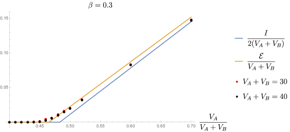
Refer to caption
Figure 25: Left: For αsubscript𝛼{{\mathcal{I}}}_{{\alpha}} given by (C.13), the logarithmic negativity is computed numerically using the resolvent (C.17) and compared to the naive analytic continuation in (4.53), (4.55) and (4.56), with excellent agreement.

Similar to the infinite temperature case, we can consider the regime where the effective dimensions dA1,dA2,dBsubscript𝑑subscript𝐴1subscript𝑑subscript𝐴2subscript𝑑𝐵d_{A_{1}},d_{A_{2}},d_{B} of the different subsystems are such that dA1dA2dB1much-less-thansubscript𝑑subscript𝐴1subscript𝑑subscript𝐴2subscript𝑑𝐵1\frac{d_{A_{1}}}{d_{A_{2}}d_{B}}\ll 1. Assuming that the same set of permutations contributes in this regime at finite temperature as the one that contributed at infinite temperature, we can then include only the first diagram from each line on the RHS of Fig. 24. We then have

Σ1=1dA+Z2,BdA(Z1,B)2R1subscriptΣ11subscript𝑑𝐴subscript𝑍2𝐵subscript𝑑𝐴superscriptsubscript𝑍1𝐵2subscript𝑅1\Sigma_{1}=\frac{1}{d_{A}}+\frac{Z_{2,B}}{d_{A}\,(Z_{1,B})^{2}}\,R_{1} (C.18)

which gives a quadratic equation

αR12+(1dAλ)R1+1=0,α=Z2,B(Z1,B)2dAformulae-sequencesuperscript𝛼superscriptsubscript𝑅121subscript𝑑𝐴𝜆subscript𝑅110superscript𝛼subscript𝑍2𝐵superscriptsubscript𝑍1𝐵2subscript𝑑𝐴\alpha^{\prime}\,R_{1}^{2}+\left(\frac{1}{d_{A}}-\lambda\right)R_{1}+1=0,\quad\alpha^{\prime}=\frac{Z_{2,B}}{(Z_{1,B})^{2}d_{A}} (C.19)

Similar to (C.10), this gives a semicircle form of the density of eigenvalues, which for this case gives

𝒵,sc(PT)={1logdA<S2,B(eq)e12(logdAS2,B(eq))logdA>S2,B(eq).subscriptsuperscript𝒵PTsccases1subscript𝑑𝐴subscriptsuperscript𝑆eq2𝐵superscript𝑒12subscript𝑑𝐴subscriptsuperscript𝑆eq2𝐵subscript𝑑𝐴subscriptsuperscript𝑆eq2𝐵{\mathcal{Z}}^{\rm(PT)}_{\infty,{\rm sc}}=\begin{cases}1&\log d_{A}<S^{\rm(eq)}_{2,B}\\ e^{\frac{1}{2}(\log d_{A}-S^{\rm(eq)}_{2,B})}&\log d_{A}>S^{\rm(eq)}_{2,B}\end{cases}\,. (C.20)

This gives the value of the logarithmic negativity we would expect in the ES phase from naive analytic continuation, and also the transition between the NE and ES phases we would expect from naive analytic continuation.

C.3.1 Toy model for black hole evaporation in JT gravity

As discussed in [1], the rules for calculating the entanglement entropy of the radiation in the holographic model of black hole evaporation in [4] can be derived from the equilibrium approximation, taking A𝐴A to be the radiation R𝑅R, B𝐵B to be the black hole, and

α=𝟏Rf(HB)eβHBsubscript𝛼tensor-productsubscript1𝑅𝑓subscript𝐻𝐵superscript𝑒𝛽subscript𝐻𝐵{{\mathcal{I}}}_{{\alpha}}=\mathbf{1}_{R}\otimes f(H_{B})e^{-\beta H_{B}} (C.21)

which is a special case of (C.13), with an additional factor f(HB)𝑓subscript𝐻𝐵f(H_{B}) which captures the effect of end-of-the-world (EOW) branes, and with the density of states as in JT gravity, so that

𝒵m,B=eS0zm(β)subscript𝒵𝑚𝐵superscript𝑒subscript𝑆0subscript𝑧𝑚𝛽\displaystyle\mathcal{Z}_{m,B}=e^{S_{0}}z_{m}(\beta) (C.22)

where S0subscript𝑆0S_{0} is the large ground state entropy and zm(β)subscript𝑧𝑚𝛽z_{m}(\beta) is O(1)𝑂1O(1). The rules for calculating 𝒵n(PT)superscriptsubscript𝒵𝑛PT{\mathcal{Z}}_{n}^{\rm(PT)} in this model can similarly be derived from the equilibrium approximation. The negativity within the radiation in this model was discussed in Refs. [55, 56].

Like in other cases, the dominant permutation in 𝒵n(PT)superscriptsubscript𝒵𝑛PT{\mathcal{Z}}_{n}^{\rm(PT)} for this choice of αsubscript𝛼{{\mathcal{I}}}_{{\alpha}} is always one out of e𝑒e, η𝜂\eta or η1superscript𝜂1\eta^{-1}, and τESsubscript𝜏𝐸𝑆\tau_{ES}. We can read off the “boundary” expressions for 𝒵n(PT)(τ)superscriptsubscript𝒵𝑛PT𝜏{\mathcal{Z}}_{n}^{\rm(PT)}(\tau) in this holographic model, in terms of dR1,dR2,Zn,Bsubscript𝑑subscript𝑅1subscript𝑑subscript𝑅2subscript𝑍𝑛𝐵d_{R_{1}},d_{R_{2}},Z_{n,B}, from the diagrams in Fig. 3 (where Zn,B=Tr[(eβHBf(HB))n]subscript𝑍𝑛𝐵Trdelimited-[]superscriptsuperscript𝑒𝛽subscript𝐻𝐵𝑓subscript𝐻𝐵𝑛Z_{n,B}=\text{Tr}[(e^{-\beta H_{B}}f(H_{B}))^{n}]). Using the relation between bulk and boundary partition functions in holography, we then find geometries like the ones shown in Fig. 26 for evaluating 𝒵n(PT)superscriptsubscript𝒵𝑛PT{\mathcal{Z}}_{n}^{\rm(PT)} in the ES and ME phases. Both involve “replica wormholes,” which are connected Euclidean gravity path integrals between multiple asymptotic boundaries. Note that more generally, (3.4) can be used to systematically derive replica wormhole prescriptions for calculating 𝒵n(PT)superscriptsubscript𝒵𝑛PT{\mathcal{Z}}_{n}^{\rm(PT)} in other gravity setups, including the model of [5].

Refer to caption
Refer to caption
Figure 26: Euclidean gravity path integrals with replica wormholes for calculating 𝒵n(PT)superscriptsubscript𝒵𝑛PT{\mathcal{Z}}_{n}^{\rm(PT)} in the model of [4], for n=4𝑛4n=4. The dominant contribution in the ES phase, shown in (a), involves connected partition functions Z2,Bsubscript𝑍2𝐵Z_{2,B} between two asymptotic boundaries, while the ME phase contribution in (b) involves Zn,Bsubscript𝑍𝑛𝐵Z_{n,B}. The black lines with arrows are asymptotic boundaries in JT gravity (each with length β𝛽\beta, although the lengths appear to differ in the figure), and the green lines are EOW branes. The dashed and dotted loops simply give factors of dA1subscript𝑑subscript𝐴1d_{A_{1}} and dA2subscript𝑑subscript𝐴2d_{A_{2}} respectively.

Note that (C.22) implies in particular that

S2,B(eq)=S0+s2(β),SB(eq)=S0+s1(β),formulae-sequencesuperscriptsubscript𝑆2𝐵eqsubscript𝑆0subscript𝑠2𝛽superscriptsubscript𝑆𝐵eqsubscript𝑆0subscript𝑠1𝛽\displaystyle S_{2,B}^{(\rm eq)}=S_{0}+s_{2}({\beta}),\quad S_{B}^{(\rm eq)}=S_{0}+s_{1}({\beta}),
s1(β)>s2(β)O(1)subscript𝑠1𝛽subscript𝑠2𝛽similar-to𝑂1\displaystyle s_{1}({\beta})>s_{2}({\beta})\sim O(1) (C.23)

From analytic continuation of the expressions for 𝒵n(PT)superscriptsubscript𝒵𝑛PT{\mathcal{Z}}_{n}^{\rm(PT)} for even n𝑛n to n1𝑛1n\rightarrow 1 in this model, the expressions for the logarithmic negativity in (4.53)-(4.55) become

NE(R1,R2)=0subscript𝑁𝐸subscript𝑅1subscript𝑅20\displaystyle{{\mathcal{E}}}_{NE}(R_{1},R_{2})=0 (C.24)
ME(R1,R2)=logdR1 or ME=logdR2formulae-sequencesubscript𝑀𝐸subscript𝑅1subscript𝑅2subscript𝑑subscript𝑅1 or subscript𝑀𝐸subscript𝑑subscript𝑅2\displaystyle{{\mathcal{E}}}_{ME}(R_{1},R_{2})=\log d_{R_{1}}\quad\text{ or }\quad{{\mathcal{E}}}_{ME}=\log d_{R_{2}} (C.25)
ES(R1,R2)=12(logdRS0s2(β)+log83π)subscript𝐸𝑆subscript𝑅1subscript𝑅212subscript𝑑𝑅subscript𝑆0subscript𝑠2𝛽83𝜋\displaystyle{{\mathcal{E}}}_{ES}(R_{1},R_{2})=\frac{1}{2}\left(\log d_{R}-S_{0}-s_{2}(\beta)+\log\frac{8}{3\pi}\right) (C.26)

Note that we have explicitly included a term log83π83𝜋\log\frac{8}{3\pi} coming from the degeneracy of the permutations in the ES phase in this case (which we have ignored for other choices of αsubscript𝛼{{\mathcal{I}}}_{{\alpha}} in the paper), as it contributes at the same order as logz2(β)z1(β)2subscript𝑧2𝛽subscript𝑧1superscript𝛽2\log\frac{z_{2}(\beta)}{z_{1}(\beta)^{2}}. Recall that the Page time tpsubscript𝑡𝑝t_{p} corresponds to c=12𝑐12c={{\frac{1}{2}}}. The transition from the NE phase, where the logarithmic negativity within the radiation is sub-extensive, to the ES phase, where it becomes extensive, takes place at

c=c012(1s1(β)s2(β)+log8π/3S0)𝑐subscript𝑐0121subscript𝑠1𝛽subscript𝑠2𝛽8𝜋3subscript𝑆0c=c_{0}\equiv\frac{1}{2}\left(1-\frac{s_{1}(\beta)-s_{2}(\beta)+\log 8\pi/3}{S_{0}}\right) (C.27)

For this model, the difference between c=12𝑐12c=\frac{1}{2} and c=c0𝑐subscript𝑐0c=c_{0} is suppressed due to the special structure of the density of states in JT gravity compared to other black hole models.

It is also interesting to consider the negativity between the black hole and a subsystem of the radiation, R1subscript𝑅1R_{1}. In this case, the permutation that dominates in 𝒵n(PT)superscriptsubscript𝒵𝑛PT{\mathcal{Z}}_{n}^{\rm(PT)} at early times when eS0dR1dR2much-greater-thansuperscript𝑒subscript𝑆0subscript𝑑subscript𝑅1subscript𝑑subscript𝑅2e^{S_{0}}\gg d_{R_{1}}d_{R_{2}} is τ=η1𝜏superscript𝜂1\tau=\eta^{-1}, leading on analytic continuation to

(R1,B)=logdR1.subscript𝑅1𝐵subscript𝑑subscript𝑅1\displaystyle\mathcal{E}(R_{1},B)=\log d_{R_{1}}. (C.28)

irrespective of the relative sizes of R1subscript𝑅1R_{1} and R2subscript𝑅2R_{2}. This means that each Hawking quantum is maximally entangled with the black hole at early times, as expected. After the Page time, if dR1dR2eS0much-greater-thansubscript𝑑subscript𝑅1subscript𝑑subscript𝑅2superscript𝑒subscript𝑆0d_{R_{1}}\gg d_{R_{2}}e^{S_{0}}, τ=η𝜏𝜂\tau=\eta dominates, and by analytic continuation the negativity is then

(R1,B)=S0+logz12(β)2z1(β)=S12,B(eq).subscript𝑅1𝐵subscript𝑆0subscript𝑧12superscript𝛽2subscript𝑧1𝛽subscriptsuperscript𝑆eq12𝐵\displaystyle\mathcal{E}(R_{1},B)=S_{0}+\log\ \frac{z_{\frac{1}{2}}(\beta)^{2}}{z_{1}(\beta)}=S^{\rm(eq)}_{\frac{1}{2},B}\,. (C.29)

Most interestingly, we can also consider the regime after the Page time where dR2dR1eS0much-greater-thansubscript𝑑subscript𝑅2subscript𝑑subscript𝑅1superscript𝑒subscript𝑆0d_{R_{2}}\gg d_{R_{1}}e^{S_{0}} i.e. how small amounts of the radiation are entangled with the black hole. The usual story of black hole evaporation says that these quanta are maximally entangled with the black hole, more specifically, their pair behind the horizon. This entanglement played a starring role in the firewall paradox [57]. But the dominant term in 𝒵n(PT)superscriptsubscript𝒵𝑛PT{\mathcal{Z}}_{n}^{\rm(PT)} is the identity, so that on analytic continuation,

(R1,B)=0.subscript𝑅1𝐵0\displaystyle\mathcal{E}(R_{1},B)=0. (C.30)

This is the statement that Hawking quanta after the Page time are not actually entangled with the black hole, but only entangled with the early radiation, avoiding paradoxes with entanglement monogamy.

Note that we can numerically compute the resolvent and spectrum in this model using the general equation (C.17), now with

ρ(E)=eS02E2π2sinh(2π2E)𝜌𝐸superscript𝑒subscript𝑆02𝐸2superscript𝜋22𝜋2𝐸\rho(E)=e^{S_{0}}\,\frac{\sqrt{2E}}{2\pi^{2}}\,\sinh(2\pi\sqrt{2E}) (C.31)

This problem is studied systematically in Ref. [56]. For the special case of the “microcanonical ensemble” in [4], the equation for the resolvent reduces to the infinite temperature case in (C.8), with the dimension of the black hole given by e𝐒superscript𝑒𝐒e^{\bf S}, where S is the microcanonical entropy of the black hole.

C.4 Microcanonical ensemble with B𝐵B at infinite temperature

We now consider αsubscript𝛼{{\mathcal{I}}}_{{\alpha}} given by (4.77), which we repeat here202020Similar resolvent calculations are done in Ref. [58].:

α=Ea1A1+Ea2A2IE,Δ|a1a1||a2a2|𝟏B.subscript𝛼subscriptsubscriptsuperscript𝐸subscript𝐴1subscript𝑎1subscriptsuperscript𝐸subscript𝐴2subscript𝑎2subscript𝐼𝐸Δtensor-producttensor-productketsubscript𝑎1brasubscript𝑎1ketsubscript𝑎2brasubscript𝑎2subscript1𝐵{{\mathcal{I}}}_{{\alpha}}=\sum_{E^{A_{1}}_{a_{1}}+E^{A_{2}}_{a_{2}}\in I_{E,\Delta}}\ket{a_{1}}\bra{a_{1}}\otimes\ket{a_{2}}\bra{a_{2}}\otimes\mathbf{1}_{B}\,. (C.32)

(i) Contributions to 𝒵n(PT)superscriptsubscript𝒵𝑛PT{\mathcal{Z}}_{n}^{\rm(PT)} from different permutations
Let us first understand the contributions to 𝒵n(PT)superscriptsubscript𝒵𝑛PT{\mathcal{Z}}_{n}^{\rm(PT)} from different permutations in this case. Recall that the contribution from τ𝜏\tau can be expanded as

ηA1ηA21eB|α,τ=i1,i1,in,inηA1ηA21eB|i1i¯1ini¯n×i1|α|iτ(1)i2|α|iτ(2)in|α|iτ(n)\displaystyle\begin{split}&{\left\langle{\eta_{A_{1}}\otimes\eta^{-1}_{A_{2}}\otimes e_{B}|{{\mathcal{I}}}_{\alpha},\tau}\right\rangle}=\sum_{i_{1},i^{\prime}_{1},...i_{n},i^{\prime}_{n}}\braket{\eta_{A_{1}}\otimes\eta^{-1}_{A_{2}}\otimes e_{B}}{i_{1}\bar{i^{\prime}}_{1}...i_{n}\bar{i^{\prime}}_{n}}\\ &\quad\quad\quad\times\braket{i_{1}}{{{\mathcal{I}}}_{{\alpha}}}{i^{\prime}_{\tau(1)}}\,\braket{i_{2}}{{{\mathcal{I}}}_{{\alpha}}}{i^{\prime}_{\tau(2)}}\,...\,\braket{i_{n}}{{{\mathcal{I}}}_{{\alpha}}}{i^{\prime}_{\tau(n)}}\end{split} (C.33)

where

|im=|imaA1|ima¯A2|imbB,|i¯m=|i¯maA1|i¯ma¯A2|i¯mbB.formulae-sequenceketsubscript𝑖𝑚subscriptketsubscript𝑖subscript𝑚𝑎subscript𝐴1subscriptketsubscript𝑖subscript𝑚¯𝑎subscript𝐴2subscriptketsubscript𝑖subscript𝑚𝑏𝐵ketsubscript¯superscript𝑖𝑚subscriptketsubscript¯superscript𝑖subscript𝑚𝑎subscript𝐴1subscriptketsubscript¯superscript𝑖subscript𝑚¯𝑎subscript𝐴2subscriptketsubscript¯superscript𝑖subscript𝑚𝑏𝐵\ket{i_{m}}=\ket{i_{m_{a}}}_{A_{1}}\ket{i_{m_{\bar{a}}}}_{A_{2}}\ket{i_{m_{b}}}_{B},\quad\ket{\bar{i^{\prime}}_{m}}=\ket{\bar{i^{\prime}}_{m_{a}}}_{A_{1}}\ket{\bar{i^{\prime}}_{m_{\bar{a}}}}_{A_{2}}\ket{\bar{i^{\prime}}_{m_{b}}}_{B}\,. (C.34)

It is useful to take the states |imaA1subscriptketsubscript𝑖subscript𝑚𝑎subscript𝐴1\ket{i_{m_{a}}}_{A_{1}}, |ima¯A2subscriptketsubscript𝑖subscript𝑚¯𝑎subscript𝐴2\ket{i_{m_{\bar{a}}}}_{A_{2}}, |imbBsubscriptketsubscript𝑖subscript𝑚𝑏𝐵\ket{i_{m_{b}}}_{B} to be energy eigenstates in A1,A2,Bsubscript𝐴1subscript𝐴2𝐵A_{1},A_{2},B. Then note that for (4.77), each factor in the second line of (C.33) simultaneously gives delta functions between the indices on A1subscript𝐴1A_{1}, A2subscript𝐴2A_{2} and B𝐵B in the bra and the ket, and enforces the condition that the energies in A1subscript𝐴1A_{1} and A2subscript𝐴2A_{2} add up to E𝐸E. For instance,

ia1ia¯1ib1|α|ia1ia¯1ib1=δia1ia1δia¯1ia¯1δib1ib1δEa1A1+Ea¯1A2,Equantum-operator-productsubscript𝑖subscript𝑎1subscript𝑖subscript¯𝑎1subscript𝑖subscript𝑏1subscript𝛼subscriptsuperscript𝑖subscript𝑎1subscriptsuperscript𝑖subscript¯𝑎1subscriptsuperscript𝑖subscript𝑏1subscript𝛿subscript𝑖subscript𝑎1subscriptsuperscript𝑖subscript𝑎1subscript𝛿subscript𝑖subscript¯𝑎1subscriptsuperscript𝑖subscript¯𝑎1subscript𝛿subscript𝑖subscript𝑏1subscriptsuperscript𝑖subscript𝑏1subscript𝛿subscriptsuperscript𝐸subscript𝐴1subscript𝑎1subscriptsuperscript𝐸subscript𝐴2subscript¯𝑎1𝐸\braket{i_{a_{1}}\,i_{\bar{a}_{1}}\,i_{b_{1}}\,}{{{\mathcal{I}}}_{{\alpha}}}{i^{\prime}_{a_{1}}\,i^{\prime}_{\bar{a}_{1}}\,i^{\prime}_{b_{1}}\,}=\delta_{i_{a_{1}}i^{\prime}_{a_{1}}}\,\delta_{i_{\bar{a}_{1}}i^{\prime}_{\bar{a}_{1}}}\,\delta_{i_{b_{1}}i^{\prime}_{b_{1}}}\delta_{E^{A_{1}}_{a_{1}}+E^{A_{2}}_{\bar{a}_{1}},\,E} (C.35)

In Fig. 27, we explain the resulting contributions from different τ𝜏\tau with the help of diagrams, showing how the energies of different index loops are related.

Refer to caption
Refer to caption
Refer to caption
Figure 27: Diagrams for different possible dominant contributions to 𝒵n(PT)superscriptsubscript𝒵𝑛PT{\mathcal{Z}}_{n}^{\rm(PT)} in the microcanonical ensemble with B𝐵B at infinite temperature. Recall that dashed, dotted and solid lines respectively represent A1subscript𝐴1A_{1}, A2subscript𝐴2A_{2}, B𝐵B. Es,Essubscript𝐸𝑠superscriptsubscript𝐸𝑠E_{s},E_{s}^{\prime} are energies in Assubscript𝐴𝑠A_{s} for s=1,2𝑠12s=1,2, and each of these energies is independently summed over in the expression for 𝒵n(PT)(τ)superscriptsubscript𝒵𝑛PT𝜏{\mathcal{Z}}_{n}^{\rm(PT)}(\tau).

Then if the density of states in subsystem P𝑃P at energy EPsubscript𝐸𝑃E_{P} is dEPPsubscriptsuperscript𝑑𝑃subscript𝐸𝑃d^{P}_{E_{P}}, we find

𝒵n(PT)(e)=1NEndBnE1dE1A1dEE1A2,superscriptsubscript𝒵𝑛PT𝑒1superscriptsubscript𝑁𝐸𝑛superscriptsubscript𝑑𝐵𝑛subscriptsubscript𝐸1subscriptsuperscript𝑑subscript𝐴1subscript𝐸1subscriptsuperscript𝑑subscript𝐴2𝐸subscript𝐸1\displaystyle{\mathcal{Z}}_{n}^{\rm(PT)}(e)=\frac{1}{N_{E}^{n}}d_{B}^{n}\sum_{E_{1}}d^{A_{1}}_{E_{1}}d^{A_{2}}_{E-E_{1}}, (C.36)
𝒵n(PT)(τES)=1NEndBn/2(E1(dE1A1)n/2dEE1A2)(E1dE1A1(dEE1A2)n/2),superscriptsubscript𝒵𝑛PTsubscript𝜏𝐸𝑆1superscriptsubscript𝑁𝐸𝑛superscriptsubscript𝑑𝐵𝑛2subscriptsubscript𝐸1superscriptsubscriptsuperscript𝑑subscript𝐴1subscript𝐸1𝑛2subscriptsuperscript𝑑subscript𝐴2𝐸subscript𝐸1subscriptsuperscriptsubscript𝐸1subscriptsuperscript𝑑subscript𝐴1subscriptsuperscript𝐸1superscriptsubscriptsuperscript𝑑subscript𝐴2𝐸subscriptsuperscript𝐸1𝑛2\displaystyle{\mathcal{Z}}_{n}^{\rm(PT)}(\tau_{ES})=\frac{1}{N_{E}^{n}}d_{B}^{n/2}\left(\sum_{E_{1}}(d^{A_{1}}_{E_{1}})^{n/2}d^{A_{2}}_{E-E_{1}}\right)\left(\sum_{{E_{1}^{\prime}}}d^{A_{1}}_{E^{\prime}_{1}}(d^{A_{2}}_{E-E^{\prime}_{1}})^{n/2}\right), (C.37)
𝒵n(PT)(η)=1NEndB(E2dE2A2(dEE2A1)n/2)(E2dE2A2(dEE2A1)n/2)superscriptsubscript𝒵𝑛PT𝜂1superscriptsubscript𝑁𝐸𝑛subscript𝑑𝐵subscriptsubscript𝐸2subscriptsuperscript𝑑subscript𝐴2subscript𝐸2superscriptsubscriptsuperscript𝑑subscript𝐴1𝐸subscript𝐸2𝑛2subscriptsubscriptsuperscript𝐸2subscriptsuperscript𝑑subscript𝐴2subscriptsuperscript𝐸2superscriptsubscriptsuperscript𝑑subscript𝐴1𝐸subscriptsuperscript𝐸2𝑛2\displaystyle{\mathcal{Z}}_{n}^{\rm(PT)}(\eta)=\frac{1}{N_{E}^{n}}d_{B}\left(\sum_{E_{2}}d^{A_{2}}_{E_{2}}(d^{A_{1}}_{E-E_{2}})^{n/2}\right)\,\left(\sum_{E^{\prime}_{2}}d^{A_{2}}_{E^{\prime}_{2}}(d^{A_{1}}_{E-E^{\prime}_{2}})^{n/2}\right) (C.38)

where

NE=Tr[α]=dBE1dE1A1dEE1A2.subscript𝑁𝐸Trdelimited-[]subscript𝛼subscript𝑑𝐵subscriptsubscript𝐸1subscriptsuperscript𝑑subscript𝐴1subscript𝐸1subscriptsuperscript𝑑subscript𝐴2𝐸subscript𝐸1N_{E}=\text{Tr}[{{\mathcal{I}}}_{{\alpha}}]=d_{B}\sum_{E_{1}}d^{A_{1}}_{E_{1}}d^{A_{2}}_{E-E_{1}}. (C.39)

On using the saddle point approximation for each of these terms, we find that the saddle point values of the energies in the resulting expressions can be identified as the saddle points that appear in expressions for Renyi entropies of equilibrium density matrices for various subsystems and indices. As a result, we can further simplify (C.36)-(C.38) to get the expressions in terms of equilibrium Renyi entropies in (4.78)-(4.81).

(ii) Resolvent and logarithmic negativity

Let us now understand what the Schwinger-Dyson equations in Fig. 23(a) and 24 give for this choice of αsubscript𝛼{{\mathcal{I}}}_{{\alpha}}. Recall that we take take |psketsubscript𝑝𝑠\ket{p_{s}}, |qsketsubscript𝑞𝑠\ket{q_{s}} to be energy eigenstates in Assubscript𝐴𝑠A_{s}. Then we can see that Rpsubscript𝑅𝑝R_{p} depends only on the energies E1subscript𝐸1E_{1} and E2subscript𝐸2E_{2} of |p1A1subscriptketsubscript𝑝1subscript𝐴1\ket{p_{1}}_{A_{1}} and |p2A2subscriptketsubscript𝑝2subscript𝐴2\ket{p_{2}}_{A_{2}}. So we can express the resolvent as a sum

RN(λ)=E1,E2dE1A1dE2A2R~(E1,E2),R~(E1,E2)={R1(E1)E1+E2=ER2(E1,E2)E1+E2Eformulae-sequencesubscript𝑅𝑁𝜆subscriptsubscript𝐸1subscript𝐸2subscriptsuperscript𝑑subscript𝐴1subscript𝐸1subscriptsuperscript𝑑subscript𝐴2subscript𝐸2~𝑅subscript𝐸1subscript𝐸2~𝑅subscript𝐸1subscript𝐸2casessubscript𝑅1subscript𝐸1subscript𝐸1subscript𝐸2𝐸subscript𝑅2subscript𝐸1subscript𝐸2subscript𝐸1subscript𝐸2𝐸R_{N}(\lambda)=\sum_{E_{1},E_{2}}d^{A_{1}}_{E_{1}}d^{A_{2}}_{E_{2}}\,\tilde{R}(E_{1},E_{2}),\quad\tilde{R}(E_{1},E_{2})=\begin{cases}R_{1}(E_{1})&E_{1}+E_{2}=E\\ R_{2}(E_{1},E_{2})&E_{1}+E_{2}\neq E\end{cases} (C.40)

The set of diagrams contributing to R~(E1,E2)~𝑅subscript𝐸1subscript𝐸2\tilde{R}(E_{1},E_{2}) differs depending on whether or not the external energies E1subscript𝐸1E_{1} and E2subscript𝐸2E_{2} add up to E𝐸E, giving the two cases R1subscript𝑅1R_{1} and R2subscript𝑅2R_{2} in (C.40). For example, out of the diagrams explicitly shown on the RHS of Fig. 23(b), in the case where E1+E2=Esubscript𝐸1subscript𝐸2𝐸E_{1}+E_{2}=E, all diagrams on the RHS of give a non-zero contribution, whereas in the case where E1+E2Esubscript𝐸1subscript𝐸2𝐸E_{1}+E_{2}\neq E, only the second diagram gives a non-zero contribution, as the remaining diagrams enforce E1+E2=Esubscript𝐸1subscript𝐸2𝐸E_{1}+E_{2}=E. Then we have

R1(E1)=1λΣ1(E1),R2(E1,E2)=1λΣ2(E1,E2)formulae-sequencesubscript𝑅1subscript𝐸11𝜆subscriptΣ1subscript𝐸1subscript𝑅2subscript𝐸1subscript𝐸21𝜆subscriptΣ2subscript𝐸1subscript𝐸2R_{1}(E_{1})=\frac{1}{\lambda-\Sigma_{1}(E_{1})},\quad R_{2}(E_{1},E_{2})=\frac{1}{\lambda-\Sigma_{2}(E_{1},E_{2})} (C.41)

where Σ1,Σ2subscriptΣ1subscriptΣ2\Sigma_{1},\Sigma_{2} are expressed in terms of R1,R2subscript𝑅1subscript𝑅2R_{1},R_{2} through the Schwinger-Dyson equations in Fig. 28 and 29.
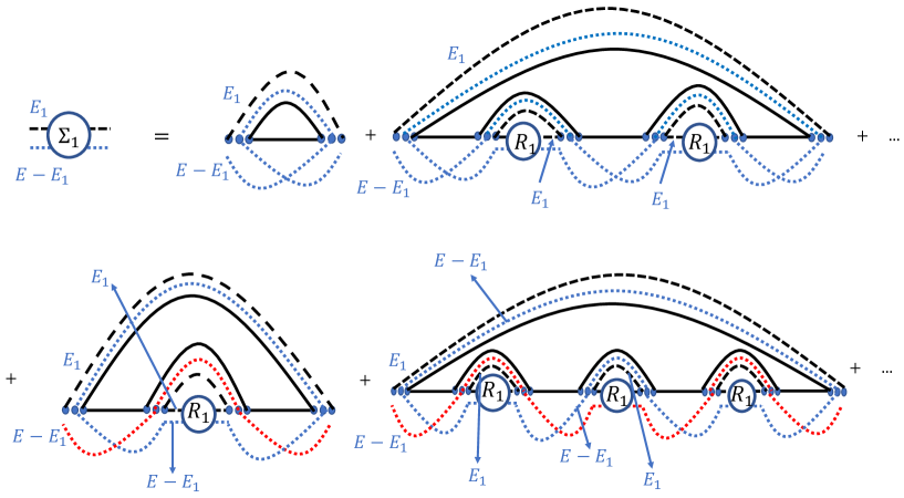
Refer to caption
Figure 28: Schwinger-Dyson equation for different contributions to Σ1(E1)subscriptΣ1subscript𝐸1\Sigma_{1}(E_{1}).
Refer to caption
Refer to caption
Figure 29: Schwinger-Dyson equation for different contributions to Σ2(E1,E2)subscriptΣ2subscript𝐸1subscript𝐸2\Sigma_{2}(E_{1},E_{2}).

Contribution from permutations with only one-cycles and two-cycles

To evaluate Σ1subscriptΣ1\Sigma_{1} and Σ2subscriptΣ2\Sigma_{2}, we can first consider the contributions from all diagrams which have only one-cycles and two-cycles, based again on the expectation that this should capture the regime where the effective dimensions are such that dA1dBdA21much-less-thansubscript𝑑subscript𝐴1subscript𝑑𝐵subscript𝑑subscript𝐴21\frac{d_{A_{1}}}{d_{B}d_{A_{2}}}\ll 1. We can restrict to such contributions by keeping only the first term in each line on the RHS of Fig. 28, and only the first term on the RHS of Fig. 29.

We then find

Σ1(E1)=dBNE+dEE1A2dE1A1dBNE2R1(E1)subscriptΣ1subscript𝐸1subscript𝑑𝐵subscript𝑁𝐸subscriptsuperscript𝑑subscript𝐴2𝐸subscript𝐸1subscriptsuperscript𝑑subscript𝐴1subscript𝐸1subscript𝑑𝐵superscriptsubscript𝑁𝐸2subscript𝑅1subscript𝐸1\Sigma_{1}(E_{1})=\frac{d_{B}}{N_{E}}+\frac{d^{A_{2}}_{E-E_{1}}d^{A_{1}}_{E_{1}}d_{B}}{N_{E}^{2}}R_{1}(E_{1}) (C.42)

which together with (C.41) gives a quadratic equation for R1subscript𝑅1R_{1},

αER12+(dBNEλ)R1+1=0,αE=dE1A1dEE1A2dBNE2formulae-sequencesubscript𝛼𝐸superscriptsubscript𝑅12subscript𝑑𝐵subscript𝑁𝐸𝜆subscript𝑅110subscript𝛼𝐸subscriptsuperscript𝑑subscript𝐴1subscript𝐸1subscriptsuperscript𝑑subscript𝐴2𝐸subscript𝐸1subscript𝑑𝐵superscriptsubscript𝑁𝐸2\alpha_{E}\,R_{1}^{2}+\left(\frac{d_{B}}{N_{E}}-\lambda\right)R_{1}+1=0,\quad\alpha_{E}=\frac{d^{A_{1}}_{E_{1}}d^{A_{2}}_{E-E_{1}}d_{B}}{N_{E}^{2}} (C.43)

which has the solution

R1(E1,EE1)=λdBNE2αE12αE(λdBNE)24αE.subscript𝑅1subscript𝐸1𝐸subscript𝐸1𝜆subscript𝑑𝐵subscript𝑁𝐸2subscript𝛼𝐸12subscript𝛼𝐸superscript𝜆subscript𝑑𝐵subscript𝑁𝐸24subscript𝛼𝐸R_{1}(E_{1},E-E_{1})=\frac{\lambda-\frac{d_{B}}{N_{E}}}{2\alpha_{E}}-\frac{1}{2\alpha_{E}}\sqrt{\left(\lambda-\frac{d_{B}}{N_{E}}\right)^{2}-4\alpha_{E}}\,. (C.44)

From the first diagram on the RHS of (29), we find

Σ2(E1,E2)=dBdEE2A1dEE1A2NE2R2(EE2,EE1)subscriptΣ2subscript𝐸1subscript𝐸2subscript𝑑𝐵subscriptsuperscript𝑑subscript𝐴1𝐸subscript𝐸2subscriptsuperscript𝑑subscript𝐴2𝐸subscript𝐸1superscriptsubscript𝑁𝐸2subscript𝑅2𝐸subscript𝐸2𝐸subscript𝐸1\Sigma_{2}(E_{1},E_{2})=\frac{d_{B}d^{A_{1}}_{E-E_{2}}d^{A_{2}}_{E-E_{1}}}{N_{E}^{2}}R_{2}(E-E_{2},E-E_{1}) (C.45)

Using the analogous equation for Σ2(EE2,EE1)subscriptΣ2𝐸subscript𝐸2𝐸subscript𝐸1\Sigma_{2}(E-E_{2},E-E_{1}) together with (C.41), we get a quadratic equation for R2(E1,E2)subscript𝑅2subscript𝐸1subscript𝐸2R_{2}(E_{1},E_{2}),

λα1R22(λ2+α1α2)R2+λ=0,α1=dE1A1dE2A2dBNE2,α2=dEE2A1dEE1A2dBNE2formulae-sequence𝜆subscript𝛼1superscriptsubscript𝑅22superscript𝜆2subscript𝛼1subscript𝛼2subscript𝑅2𝜆0formulae-sequencesubscript𝛼1subscriptsuperscript𝑑subscript𝐴1subscript𝐸1subscriptsuperscript𝑑subscript𝐴2subscript𝐸2subscript𝑑𝐵superscriptsubscript𝑁𝐸2subscript𝛼2subscriptsuperscript𝑑subscript𝐴1𝐸subscript𝐸2subscriptsuperscript𝑑subscript𝐴2𝐸subscript𝐸1subscript𝑑𝐵superscriptsubscript𝑁𝐸2\lambda\alpha_{1}R_{2}^{2}-(\lambda^{2}+\alpha_{1}-\alpha_{2})R_{2}+\lambda=0,\quad\alpha_{1}=\frac{d^{A_{1}}_{E_{1}}d^{A_{2}}_{E_{2}}d_{B}}{N_{E}^{2}},~{}~{}\alpha_{2}=\frac{d^{A_{1}}_{E-E_{2}}d^{A_{2}}_{E-E_{1}}d_{B}}{N_{E}^{2}}\, (C.46)

which has the solution

R2(E1,E2)=λ2+α1α2(λa1)(λa2)(λ+a2)(λ+a1)2λα1subscript𝑅2subscript𝐸1subscript𝐸2superscript𝜆2subscript𝛼1subscript𝛼2𝜆subscript𝑎1𝜆subscript𝑎2𝜆subscript𝑎2𝜆subscript𝑎12𝜆subscript𝛼1R_{2}(E_{1},E_{2})=\frac{\lambda^{2}+\alpha_{1}-\alpha_{2}-\sqrt{(\lambda-a_{1})(\lambda-a_{2})(\lambda+a_{2})(\lambda+a_{1})}}{2\lambda\alpha_{1}} (C.47)

where

a1=α1+α2,a2=|α1α2|.formulae-sequencesubscript𝑎1subscript𝛼1subscript𝛼2subscript𝑎2subscript𝛼1subscript𝛼2\quad a_{1}=\sqrt{\alpha_{1}}+\sqrt{\alpha_{2}},\quad a_{2}=|\sqrt{\alpha_{1}}-\sqrt{\alpha_{2}}|\,. (C.48)

By substituting R1subscript𝑅1R_{1} and R2subscript𝑅2R_{2} back into (C.40) and finding the imaginary part, we can find the density of eigenvalues of ρAT2superscriptsubscript𝜌𝐴subscript𝑇2\rho_{A}^{T_{2}}:

DN(λ)=E11pE1Dsc(λ~,dE1A1dEE1A2,dB)+E1E2DE1,E2(λ)subscript𝐷𝑁𝜆subscriptsubscript𝐸11subscript𝑝subscript𝐸1superscriptsubscript𝐷sc~𝜆subscriptsuperscript𝑑subscript𝐴1subscript𝐸1subscriptsuperscript𝑑subscript𝐴2𝐸subscript𝐸1subscript𝑑𝐵subscriptsubscript𝐸1subscript𝐸2subscript𝐷subscript𝐸1subscript𝐸2𝜆D_{N}(\lambda)=\sum_{E_{1}}\frac{1}{p_{E_{1}}}D_{\infty}^{\rm sc}(\tilde{\lambda},d^{A_{1}}_{E_{1}}d^{A_{2}}_{E-E_{1}},d_{B})+\sum_{E_{1}\neq E_{2}}D_{E_{1},E_{2}}(\lambda) (C.49)

where the first term is expressed in terms of the infinite temperature value of DN(λ)subscript𝐷𝑁𝜆D_{N}(\lambda) in the semi-circle regime from (C.11), and we have introduced

pE1=dE1A1dEE1A2dBNE,λ~=λpE1.formulae-sequencesubscript𝑝subscript𝐸1subscriptsuperscript𝑑subscript𝐴1subscript𝐸1subscriptsuperscript𝑑subscript𝐴2𝐸subscript𝐸1subscript𝑑𝐵subscript𝑁𝐸~𝜆𝜆subscript𝑝subscript𝐸1p_{E_{1}}=\frac{d^{A_{1}}_{E_{1}}d^{A_{2}}_{E-E_{1}}d_{B}}{N_{E}},\quad\tilde{\lambda}=\frac{\lambda}{p_{E_{1}}}\,. (C.50)

The second term of (C.49) is found by noting that the second term in (C.47) is imaginary between a1subscript𝑎1-a_{1} and a2subscript𝑎2-a_{2}, and between a2subscript𝑎2a_{2} and a1subscript𝑎1a_{1},

DE1,E2(λ)=12(dE1A1dE2A2dEE2A1dEE1A2)δ(λ)+NE22π|λ|dBa12λ2λ2a22θ(a12λ2)θ(λ2a22)subscript𝐷subscript𝐸1subscript𝐸2𝜆12subscriptsuperscript𝑑subscript𝐴1subscript𝐸1subscriptsuperscript𝑑subscript𝐴2subscript𝐸2subscriptsuperscript𝑑subscript𝐴1𝐸subscript𝐸2subscriptsuperscript𝑑subscript𝐴2𝐸subscript𝐸1𝛿𝜆superscriptsubscript𝑁𝐸22𝜋𝜆subscript𝑑𝐵superscriptsubscript𝑎12superscript𝜆2superscript𝜆2superscriptsubscript𝑎22𝜃superscriptsubscript𝑎12superscript𝜆2𝜃superscript𝜆2superscriptsubscript𝑎22\begin{gathered}D_{E_{1},E_{2}}(\lambda)=\frac{1}{2}(d^{A_{1}}_{E_{1}}d^{A_{2}}_{E_{2}}-d^{A_{1}}_{E-E_{2}}d^{A_{2}}_{E-E_{1}})\delta(\lambda)\\ +\frac{N_{E}^{2}}{2\pi|\lambda|d_{B}}\,\sqrt{a_{1}^{2}-\lambda^{2}}\sqrt{\lambda^{2}-a_{2}^{2}}\,\theta(a_{1}^{2}-\lambda^{2})\theta(\lambda^{2}-a_{2}^{2})\end{gathered} (C.51)

So the exponential of the logarithmic negativity, i|λi|subscript𝑖subscript𝜆𝑖\sum_{i}|\lambda_{i}|, is given by

𝒵(PT)=E1pE1𝒵,sc(PT)(dE1A1dEE1A2,dB)+E1,E2NE2πdBa2a1𝑑λa12λ2λ2a22superscript𝒵PTsubscriptsubscript𝐸1subscript𝑝subscript𝐸1subscriptsuperscript𝒵PTscsubscriptsuperscript𝑑subscript𝐴1subscript𝐸1subscriptsuperscript𝑑subscript𝐴2𝐸subscript𝐸1subscript𝑑𝐵subscriptsubscript𝐸1subscript𝐸2superscriptsubscript𝑁𝐸2𝜋subscript𝑑𝐵superscriptsubscriptsubscript𝑎2subscript𝑎1differential-d𝜆superscriptsubscript𝑎12superscript𝜆2superscript𝜆2superscriptsubscript𝑎22{\mathcal{Z}}^{\rm(PT)}=\sum_{E_{1}}p_{E_{1}}{\mathcal{Z}}^{\rm(PT)}_{\infty,\,{\rm sc}}(d^{A_{1}}_{E_{1}}d^{A_{2}}_{E-E_{1}},d_{B})+\sum_{E_{1},E_{2}}\frac{N_{E}^{2}}{\pi d_{B}}\int_{a_{2}}^{a_{1}}d\lambda\sqrt{a_{1}^{2}-\lambda^{2}}\sqrt{\lambda^{2}-a_{2}^{2}} (C.52)

where 𝒵,sc(PT)subscriptsuperscript𝒵PTsc{\mathcal{Z}}^{\rm(PT)}_{\infty,{\rm sc}} is given by (C.20).

The integral in (C.52) evaluates to

a2a1𝑑λa12λ2λ2a22=23a13E(1a22a12)+23a1a22E(1a22a12)43a1a22K(1a22a12)superscriptsubscriptsubscript𝑎2subscript𝑎1differential-d𝜆superscriptsubscript𝑎12superscript𝜆2superscript𝜆2superscriptsubscript𝑎2223superscriptsubscript𝑎13𝐸1superscriptsubscript𝑎22superscriptsubscript𝑎1223subscript𝑎1superscriptsubscript𝑎22𝐸1superscriptsubscript𝑎22superscriptsubscript𝑎1243subscript𝑎1superscriptsubscript𝑎22𝐾1superscriptsubscript𝑎22superscriptsubscript𝑎12\int_{a_{2}}^{a_{1}}d\lambda\sqrt{a_{1}^{2}-\lambda^{2}}\sqrt{\lambda^{2}-a_{2}^{2}}=\frac{2}{3}a_{1}^{3}\,E\left(1-\frac{a_{2}^{2}}{a_{1}^{2}}\right)+\frac{2}{3}a_{1}a_{2}^{2}\,E\left(1-\frac{a_{2}^{2}}{a_{1}^{2}}\right)-\frac{4}{3}a_{1}a_{2}^{2}\,K\left(1-\frac{a_{2}^{2}}{a_{1}^{2}}\right) (C.53)

where K𝐾K and E𝐸E respectively refer to complete elliptic integrals of the first and second kind. Now since a2/a11+ecV+subscript𝑎2subscript𝑎11superscript𝑒𝑐𝑉a_{2}/a_{1}\approx 1+e^{-cV}+... for some positive coefficient c𝑐c, to find the leading contribution in volume we can approximate both of the elliptic functions appearing above with the leading orders in their Taylor expansions as their argument goes to 0, which are both given by π/2𝜋2\pi/2. We can then approximate

a2a1𝑑λa12λ2λ2a22π3a1(a12a22)=4π3(α1+α2)α1α2superscriptsubscriptsubscript𝑎2subscript𝑎1differential-d𝜆superscriptsubscript𝑎12superscript𝜆2superscript𝜆2superscriptsubscript𝑎22𝜋3subscript𝑎1superscriptsubscript𝑎12superscriptsubscript𝑎224𝜋3subscript𝛼1subscript𝛼2subscript𝛼1subscript𝛼2\int_{a_{2}}^{a_{1}}d\lambda\sqrt{a_{1}^{2}-\lambda^{2}}\sqrt{\lambda^{2}-a_{2}^{2}}\approx\frac{\pi}{3}a_{1}\left(a_{1}^{2}-a_{2}^{2}\right)=\frac{4\pi}{3}(\sqrt{\alpha_{1}}+\sqrt{\alpha_{2}})\sqrt{\alpha_{1}\,\alpha_{2}} (C.54)

So we find

𝒵(PT)=dBNEE1,dE1A1dEE1A2<dBdE1A1dEE1A2+dBNEE1,dE1A1dEE1A2>dB(dE1A1)3/2(dEE1A2)3/2+83dBNEE1dE1A1(dEE1A2)12×E2dE2A2(dEE2A1)12superscript𝒵PTsubscript𝑑𝐵subscript𝑁𝐸subscriptsubscript𝐸1subscriptsuperscript𝑑subscript𝐴1subscript𝐸1subscriptsuperscript𝑑subscript𝐴2𝐸subscript𝐸1subscript𝑑𝐵subscriptsuperscript𝑑subscript𝐴1subscript𝐸1subscriptsuperscript𝑑subscript𝐴2𝐸subscript𝐸1subscript𝑑𝐵subscript𝑁𝐸subscriptsubscript𝐸1subscriptsuperscript𝑑subscript𝐴1subscript𝐸1subscriptsuperscript𝑑subscript𝐴2𝐸subscript𝐸1subscript𝑑𝐵superscriptsubscriptsuperscript𝑑subscript𝐴1subscript𝐸132superscriptsubscriptsuperscript𝑑subscript𝐴2𝐸subscript𝐸13283subscript𝑑𝐵subscript𝑁𝐸subscriptsubscript𝐸1subscriptsuperscript𝑑subscript𝐴1subscript𝐸1superscriptsubscriptsuperscript𝑑subscript𝐴2𝐸subscript𝐸112subscriptsubscript𝐸2subscriptsuperscript𝑑subscript𝐴2subscript𝐸2superscriptsubscriptsuperscript𝑑subscript𝐴1𝐸subscript𝐸212\begin{gathered}{\mathcal{Z}}^{\rm(PT)}=\frac{d_{B}}{N_{E}}\sum_{E_{1},\,d^{A_{1}}_{E_{1}}d^{A_{2}}_{E-E_{1}}<d_{B}}d^{A_{1}}_{E_{1}}d^{A_{2}}_{E-E_{1}}+\frac{\sqrt{d_{B}}}{N_{E}}\sum_{E_{1},\,d^{A_{1}}_{E_{1}}d^{A_{2}}_{E-E_{1}}>d_{B}}(d^{A_{1}}_{E_{1}})^{3/2}(d^{A_{2}}_{E-E_{1}})^{3/2}\\ +\frac{8}{3}\frac{\sqrt{d_{B}}}{N_{E}}\,\sum_{E_{1}}d^{A_{1}}_{E_{1}}\left(d^{A_{2}}_{E-E_{1}}\right)^{\frac{1}{2}}\,\times\,\sum_{E_{2}}d^{A_{2}}_{E_{2}}\left(d^{A_{1}}_{E-E_{2}}\right)^{\frac{1}{2}}\end{gathered} (C.55)

The saddle point energy density for the first two terms in the last line is the same, and is equal to ϵ=E/VAitalic-ϵ𝐸subscript𝑉𝐴\epsilon=E/V_{A}. When c=SA(eq)SA(eq)+SB(eq)<12𝑐subscriptsuperscript𝑆eq𝐴subscriptsuperscript𝑆eq𝐴subscriptsuperscript𝑆eq𝐵12c=\frac{S^{\rm(eq)}_{A}}{S^{\rm(eq)}_{A}+S^{\rm(eq)}_{B}}<\frac{1}{2}, this saddle point lies in the regime of the first term, which then contributes 1. The contribution from the second term is given by its boundary value in this regime, which is always less than the saddle-point value of the same expression, given by e12(SA1(eq)+SA2(eq)SB(eq))superscript𝑒12subscriptsuperscript𝑆eqsubscript𝐴1subscriptsuperscript𝑆eqsubscript𝐴2subscriptsuperscript𝑆eq𝐵e^{\frac{1}{2}(S^{\rm(eq)}_{A_{1}}+S^{\rm(eq)}_{A_{2}}-S^{\rm(eq)}_{B})}. For c>12𝑐12c>\frac{1}{2}, the second term contributes e12(SA1(eq)+SA2(eq)SB(eq))superscript𝑒12subscriptsuperscript𝑆eqsubscript𝐴1subscriptsuperscript𝑆eqsubscript𝐴2subscriptsuperscript𝑆eq𝐵e^{\frac{1}{2}(S^{\rm(eq)}_{A_{1}}+S^{\rm(eq)}_{A_{2}}-S^{\rm(eq)}_{B})} and dominates over the first. The last term can always be approximated with its saddle point value, which is given by e12(S12,A1(eq)+S12,A2(eq)SB(eq))superscript𝑒12subscriptsuperscript𝑆eq12subscript𝐴1subscriptsuperscript𝑆eq12subscript𝐴2subscriptsuperscript𝑆eq𝐵e^{{\frac{1}{2}(S^{\rm(eq)}_{\frac{1}{2},A_{1}}+S^{\rm(eq)}_{\frac{1}{2},A_{2}}-S^{\rm(eq)}_{B})}} (where we have ignored an overall factor that gives an O(1)𝑂1O(1) contribution to negativity). For S12,A1(eq)+S12,A2(eq)>SB(eq)subscriptsuperscript𝑆eq12subscript𝐴1subscriptsuperscript𝑆eq12subscript𝐴2subscriptsuperscript𝑆eq𝐵S^{\rm(eq)}_{{{\frac{1}{2}}},A_{1}}+S^{\rm(eq)}_{{{\frac{1}{2}}},A_{2}}>S^{\rm(eq)}_{B}, this contribution dominates over the other two terms, giving

=12(S12,A1(eq)+S12,A2(eq)SB(eq))12subscriptsuperscript𝑆eq12subscript𝐴1subscriptsuperscript𝑆eq12subscript𝐴2subscriptsuperscript𝑆eq𝐵{{\mathcal{E}}}=\frac{1}{2}\left(S^{\rm(eq)}_{\frac{1}{2},A_{1}}+S^{\rm(eq)}_{\frac{1}{2},A_{2}}-S^{\rm(eq)}_{B}\right) (C.56)

Both the ES phase value of the negativity (C.56) and the transition line S12,A1(eq)+S12,A2(eq)=SB(eq)subscriptsuperscript𝑆eq12subscript𝐴1subscriptsuperscript𝑆eq12subscript𝐴2subscriptsuperscript𝑆eq𝐵S^{\rm(eq)}_{{{\frac{1}{2}}},A_{1}}+S^{\rm(eq)}_{{{\frac{1}{2}}},A_{2}}=S^{\rm(eq)}_{B} in this approximation thus agree with the naive analytic continuation in (4.84) and (4.86).

Contribution from all planar permutations

Let us now sum over all contributions on the RHS of Figs. 28 and 29. While in this case we are not able to find the logarithmic negativity in all regimes from this calculation either analytically or numerically, we can use the expression for the full sum to systematically understand the regime in which the above result from all permutations with only one- and two- cycles should be valid.

On the RHS of Fig. 28(b), each of the two lines can be obtained by summing over a geometric series, so that we get

Σ1=(dBNE+αER1)11βER12,βE=(dE1A1)2NE2formulae-sequencesubscriptΣ1subscript𝑑𝐵subscript𝑁𝐸subscript𝛼𝐸subscript𝑅111subscript𝛽𝐸superscriptsubscript𝑅12subscript𝛽𝐸superscriptsubscriptsuperscript𝑑subscript𝐴1subscript𝐸12superscriptsubscript𝑁𝐸2\Sigma_{1}=\left(\frac{d_{B}}{N_{E}}+\alpha_{E}\,R_{1}\right)\frac{1}{1-\beta_{E}\,R_{1}^{2}},\quad\beta_{E}=\frac{(d^{A_{1}}_{E_{1}})^{2}}{N_{E}^{2}} (C.57)

Here we have suppressed the arguments of both Σ1subscriptΣ1\Sigma_{1} and R1subscript𝑅1R_{1}, which are the same in all expressions. This gives a cubic equation for R1(E1)subscript𝑅1subscript𝐸1R_{1}(E_{1}):

βEλR13+(αEβE)R12+(dBNEλ)R1+1=0.subscript𝛽𝐸𝜆superscriptsubscript𝑅13subscript𝛼𝐸subscript𝛽𝐸superscriptsubscript𝑅12subscript𝑑𝐵subscript𝑁𝐸𝜆subscript𝑅110\beta_{E}\lambda R_{1}^{3}+(\alpha_{E}-\beta_{E})R_{1}^{2}+\left(\frac{d_{B}}{N_{E}}-\lambda\right)R_{1}+1=0\,. (C.58)

We see that this reduces to the contribution from only one-cycles and two-cycles in (C.43) when αEβEmuch-greater-thansubscript𝛼𝐸subscript𝛽𝐸\alpha_{E}\gg\beta_{E} for all E1subscript𝐸1E_{1}, i.e. when

dEE1A2dBdE1A1,for all E1.much-greater-thansubscriptsuperscript𝑑subscript𝐴2𝐸subscript𝐸1subscript𝑑𝐵subscriptsuperscript𝑑subscript𝐴1subscript𝐸1for all E1d^{A_{2}}_{E-E_{1}}d_{B}\gg d^{A_{1}}_{E_{1}},\quad\text{for all $E_{1}$}\,. (C.59)

Comparing this to the cubic equation for the infinite temperature case (C.8), we find that the first term in (C.40) is given by

E1dE1A1dEE1A2R1(E1,EE1)=E11pE1RN(dE1A1,dEE1A2,dB)subscriptsubscript𝐸1subscriptsuperscript𝑑subscript𝐴1subscript𝐸1subscriptsuperscript𝑑subscript𝐴2𝐸subscript𝐸1subscript𝑅1subscript𝐸1𝐸subscript𝐸1subscriptsubscript𝐸11subscript𝑝subscript𝐸1superscriptsubscript𝑅𝑁subscriptsuperscript𝑑subscript𝐴1subscript𝐸1subscriptsuperscript𝑑subscript𝐴2𝐸subscript𝐸1subscript𝑑𝐵\sum_{E_{1}}d^{A_{1}}_{E_{1}}d^{A_{2}}_{E-E_{1}}R_{1}(E_{1},E-E_{1})=\sum_{E_{1}}\frac{1}{p_{E_{1}}}R_{N}^{\infty}(d^{A_{1}}_{E_{1}},d^{A_{2}}_{E-E_{1}},d_{B}) (C.60)

where RNsuperscriptsubscript𝑅𝑁R_{N}^{\infty} is the infinite temperature resolvent. The contribution to 𝒵(PT)superscript𝒵PT{\mathcal{Z}}^{\rm(PT)} from this term is therefore

𝒵1(PT)=E1pE1𝒵(PT)(dE1A1,dEE1A2,dB).subscriptsuperscript𝒵PT1subscriptsubscript𝐸1subscript𝑝subscript𝐸1subscriptsuperscript𝒵PTsubscriptsuperscript𝑑subscript𝐴1subscript𝐸1subscriptsuperscript𝑑subscript𝐴2𝐸subscript𝐸1subscript𝑑𝐵{\mathcal{Z}}^{\rm(PT)}_{1}=\sum_{E_{1}}p_{E_{1}}{\mathcal{Z}}^{\rm(PT)}_{\infty}(d^{A_{1}}_{E_{1}},d^{A_{2}}_{E-E_{1}},d_{B})\,. (C.61)

Now for evaluating Σ2subscriptΣ2\Sigma_{2}, the RHS of (29) also gives a geometric series (suppressing the λ𝜆\lambda argument in all Σ2subscriptΣ2\Sigma_{2}, R2subscript𝑅2R_{2} below):

Σ2(E1,E2)=dEE2A1dEE1A2dBNE2R2(EE2,EE1)(1+Δ~+Δ~2+),Δ~=dE1A1dEE2A1NE2R(E1,E2)R(EE2,EE1)formulae-sequencesubscriptΣ2subscript𝐸1subscript𝐸2subscriptsuperscript𝑑subscript𝐴1𝐸subscript𝐸2subscriptsuperscript𝑑subscript𝐴2𝐸subscript𝐸1subscript𝑑𝐵superscriptsubscript𝑁𝐸2subscript𝑅2𝐸subscript𝐸2𝐸subscript𝐸11~Δsuperscript~Δ2~Δsubscriptsuperscript𝑑subscript𝐴1subscript𝐸1subscriptsuperscript𝑑subscript𝐴1𝐸subscript𝐸2superscriptsubscript𝑁𝐸2𝑅subscript𝐸1subscript𝐸2𝑅𝐸subscript𝐸2𝐸subscript𝐸1\begin{gathered}\Sigma_{2}(E_{1},E_{2})=\frac{d^{A_{1}}_{E-E_{2}}d^{A_{2}}_{E-E_{1}}d_{B}}{N_{E}^{2}}R_{2}(E-E_{2},E-E_{1})(1+\tilde{\Delta}+\tilde{\Delta}^{2}+...),\\ \tilde{\Delta}=\frac{d^{A_{1}}_{E_{1}}d^{A_{1}}_{E-E_{2}}}{N_{E}^{2}}R(E_{1},E_{2})R(E-E_{2},E-E_{1})\end{gathered} (C.62)

To simplify the notation, let us fix some E1subscript𝐸1E_{1} and E2subscript𝐸2E_{2}, and denote

Σ2:=Σ2(E1,E2),Σ2:=Σ2(EE2,EE1),R2:=Σ2(E1,E2),R2:=R2(EE2,EE1)formulae-sequenceassignsubscriptΣ2subscriptΣ2subscript𝐸1subscript𝐸2formulae-sequenceassignsuperscriptsubscriptΣ2subscriptΣ2𝐸subscript𝐸2𝐸subscript𝐸1formulae-sequenceassignsubscript𝑅2subscriptΣ2subscript𝐸1subscript𝐸2assignsuperscriptsubscript𝑅2subscript𝑅2𝐸subscript𝐸2𝐸subscript𝐸1\Sigma_{2}:=\Sigma_{2}(E_{1},E_{2}),\quad\Sigma_{2}^{\prime}:=\Sigma_{2}(E-E_{2},E-E_{1}),\quad R_{2}:=\Sigma_{2}(E_{1},E_{2}),\quad R_{2}^{\prime}:=R_{2}(E-E_{2},E-E_{1}) (C.63)

Then from (C.62) and (C.41), we have

λ1R2=Σ2=dEE2A1dEE1A2dBNE2R211dE1A1dEE2A1NE2R2R2𝜆1subscript𝑅2subscriptΣ2subscriptsuperscript𝑑subscript𝐴1𝐸subscript𝐸2subscriptsuperscript𝑑subscript𝐴2𝐸subscript𝐸1subscript𝑑𝐵superscriptsubscript𝑁𝐸2subscriptsuperscript𝑅211subscriptsuperscript𝑑subscript𝐴1subscript𝐸1subscriptsuperscript𝑑subscript𝐴1𝐸subscript𝐸2superscriptsubscript𝑁𝐸2subscript𝑅2superscriptsubscript𝑅2\displaystyle\lambda-\frac{1}{R_{2}}=\Sigma_{2}=\frac{d^{A_{1}}_{E-E_{2}}d^{A_{2}}_{E-E_{1}}d_{B}}{N_{E}^{2}}\,R^{\prime}_{2}\,\frac{1}{1-\frac{d^{A_{1}}_{E_{1}}d^{A_{1}}_{E-E_{2}}}{N_{E}^{2}}R_{2}R_{2}^{\prime}} (C.64)
λ1R2=Σ2=dE1A1dE2A2dBNE2R211dEE2A1dE1A1NE2R2R2𝜆1subscriptsuperscript𝑅2subscriptsuperscriptΣ2subscriptsuperscript𝑑subscript𝐴1subscript𝐸1subscriptsuperscript𝑑subscript𝐴2subscript𝐸2subscript𝑑𝐵superscriptsubscript𝑁𝐸2subscript𝑅211subscriptsuperscript𝑑subscript𝐴1𝐸subscript𝐸2subscriptsuperscript𝑑subscript𝐴1subscript𝐸1superscriptsubscript𝑁𝐸2subscript𝑅2superscriptsubscript𝑅2\displaystyle\lambda-\frac{1}{R^{\prime}_{2}}=\Sigma^{\prime}_{2}=\frac{d^{A_{1}}_{E_{1}}d^{A_{2}}_{E_{2}}d_{B}}{N_{E}^{2}}R_{2}\,\frac{1}{1-\frac{d^{A_{1}}_{E-E_{2}}d^{A_{1}}_{E_{1}}}{N_{E}^{2}}R_{2}R_{2}^{\prime}} (C.65)

From (C.64) and (C.65), we get the following cubic equation for R2subscript𝑅2R_{2}:

α3λ2R23+λ(α4+α12α3)R22(λ2+α4α3α2+α1)R2+λ=0.subscript𝛼3superscript𝜆2superscriptsubscript𝑅23𝜆subscript𝛼4subscript𝛼12subscript𝛼3superscriptsubscript𝑅22superscript𝜆2subscript𝛼4subscript𝛼3subscript𝛼2subscript𝛼1subscript𝑅2𝜆0\alpha_{3}\lambda^{2}R_{2}^{3}+\lambda(\alpha_{4}+\alpha_{1}-2\alpha_{3})R_{2}^{2}-(\lambda^{2}+\alpha_{4}-\alpha_{3}-\alpha_{2}+\alpha_{1})R_{2}+\lambda=0\,. (C.66)

where

α3=(dE1A1)2dE2A2dEE1A2NE2,α4=dE1A1dEE2A1NE2,formulae-sequencesubscript𝛼3superscriptsubscriptsuperscript𝑑subscript𝐴1subscript𝐸12subscriptsuperscript𝑑subscript𝐴2subscript𝐸2subscriptsuperscript𝑑subscript𝐴2𝐸subscript𝐸1superscriptsubscript𝑁𝐸2subscript𝛼4subscriptsuperscript𝑑subscript𝐴1subscript𝐸1subscriptsuperscript𝑑subscript𝐴1𝐸subscript𝐸2superscriptsubscript𝑁𝐸2\alpha_{3}=\frac{(d^{A_{1}}_{E_{1}})^{2}d^{A_{2}}_{E_{2}}}{d^{A_{2}}_{E-E_{1}}N_{E}^{2}},\quad\alpha_{4}=\frac{d^{A_{1}}_{E_{1}}d^{A_{1}}_{E-E_{2}}}{N_{E}^{2}}, (C.67)

and α1,α2subscript𝛼1subscript𝛼2\alpha_{1},\alpha_{2} were defined in (C.46). This reduces to the contribution from one-cycles and two-cycles in (C.46) if α1α3,α1α4formulae-sequencemuch-greater-thansubscript𝛼1subscript𝛼3much-greater-thansubscript𝛼1subscript𝛼4\alpha_{1}\gg\alpha_{3},~{}~{}\alpha_{1}\gg\alpha_{4}, i.e. if we have (C.59) and the additional condition

dE1A2dBdEE1A2for all E1.much-greater-thansubscriptsuperscript𝑑subscript𝐴2subscript𝐸1subscript𝑑𝐵subscriptsuperscript𝑑subscript𝐴2𝐸subscript𝐸1for all subscript𝐸1d^{A_{2}}_{E_{1}}\,d_{B}\gg d^{A_{2}}_{E-E_{1}}\quad{\text{for all }E_{1}.} (C.68)

The solutions to this equation are

R2=2abc3aλ+eqi2π/36aλ221/3Z(X+Y)1/3+eiq2π/36aλ222/3(X+Y)1/3subscript𝑅22𝑎𝑏𝑐3𝑎𝜆superscript𝑒𝑞𝑖2𝜋36𝑎superscript𝜆2superscript213𝑍superscript𝑋𝑌13superscript𝑒𝑖𝑞2𝜋36𝑎superscript𝜆2superscript223superscript𝑋𝑌13R_{2}=\frac{2a-b-c}{3a\lambda}+\frac{e^{-qi2\pi/3}}{6a\lambda^{2}}2^{1/3}\frac{Z}{(X+\sqrt{Y})^{1/3}}+\frac{e^{iq2\pi/3}}{6a\lambda^{2}}2^{2/3}(X+\sqrt{Y})^{1/3} (C.69)

with q=0,1,1𝑞011q=0,1,-1, and

X=λ3(9a(a+b+c)λ2(2abc)(a22(b+c)2a(b+c9d)))Z=λ2(6aλ2+2(a2+(b+c)2a(b+c+3d)))Y=X2Z32𝑋superscript𝜆39𝑎𝑎𝑏𝑐superscript𝜆22𝑎𝑏𝑐superscript𝑎22superscript𝑏𝑐2𝑎𝑏𝑐9𝑑𝑍superscript𝜆26𝑎superscript𝜆22superscript𝑎2superscript𝑏𝑐2𝑎𝑏𝑐3𝑑𝑌superscript𝑋2superscript𝑍32\begin{gathered}X=\lambda^{3}(-9a(a+b+c)\lambda^{2}-(2a-b-c)(a^{2}-2(b+c)^{2}-a(b+c-9d)))\\ Z=\lambda^{2}(6a\lambda^{2}+2(a^{2}+(b+c)^{2}-a(b+c+3d)))\\ Y=X^{2}-\frac{Z^{3}}{2}\\ \end{gathered} (C.70)

In the limit λ𝜆\lambda\rightarrow\infty,

Z6aλ4(1+O(1λ2)),(X+Y)1/3=eiπ/621/33a1/2λ2(1+ia(a+b+c)23a3/2λ)formulae-sequence𝑍6𝑎superscript𝜆41𝑂1superscript𝜆2superscript𝑋𝑌13superscript𝑒𝑖𝜋6superscript2133superscript𝑎12superscript𝜆21𝑖𝑎𝑎𝑏𝑐23superscript𝑎32𝜆\begin{gathered}Z\rightarrow 6a\lambda^{4}(1+O(\frac{1}{\lambda^{2}})),\\ (X+\sqrt{Y})^{1/3}=e^{i\pi/6}2^{1/3}\sqrt{3}a^{1/2}\lambda^{2}(1+i\frac{a(a+b+c)}{2\sqrt{3}a^{3/2}\lambda})\end{gathered} (C.71)

and hence

R2=2abc3aλ+ei(2πq3+π6)3a(1ia+b+c23a3/2λ)+ei(2πq3+π6)3a(1+ia+b+c23a3/2λ)+O(1λ2)subscript𝑅22𝑎𝑏𝑐3𝑎𝜆superscript𝑒𝑖2𝜋𝑞3𝜋63𝑎1𝑖𝑎𝑏𝑐23superscript𝑎32𝜆superscript𝑒𝑖2𝜋𝑞3𝜋63𝑎1𝑖𝑎𝑏𝑐23superscript𝑎32𝜆𝑂1superscript𝜆2R_{2}=\frac{2a-b-c}{3a\lambda}+\frac{e^{-i(\frac{2\pi q}{3}+\frac{\pi}{6})}}{\sqrt{3}\sqrt{a}}(1-i\frac{a+b+c}{2\sqrt{3}a^{3/2}\lambda})+\frac{e^{i(\frac{2\pi q}{3}+\frac{\pi}{6})}}{\sqrt{3}\sqrt{a}}(1+i\frac{a+b+c}{2\sqrt{3}a^{3/2}\lambda})+O\left(\frac{1}{\lambda^{2}}\right) (C.72)

For the solutions with q=0,1𝑞01q=0,1, the leading order in the λ𝜆\lambda\rightarrow\infty limit is O(λ0)𝑂superscript𝜆0O(\lambda^{0}), which implies that the leading behaviour of R𝑅R coming from these solutions is also O(λ0)𝑂superscript𝜆0O(\lambda^{0}). Since R𝑅R should approach dAλsubscript𝑑𝐴𝜆\frac{d_{A}}{\lambda}, these solutions are not allowed. For q=1𝑞1q=-1, we find in this limit

R2(λ)=1λ+O(1λ2)subscript𝑅2𝜆1𝜆𝑂1superscript𝜆2R_{2}(\lambda)=\frac{1}{\lambda}+O(\frac{1}{\lambda^{2}}) (C.73)

R1(E1;λ)subscript𝑅1subscript𝐸1𝜆R_{1}(E_{1};\lambda) also approaches 1λ1𝜆\frac{1}{\lambda}. We therefore find

RN(λ)=E1,E2dE1A1dE2A2λ+O(1λ2)=dAλ+O(1λ2)subscript𝑅𝑁𝜆subscriptsubscript𝐸1subscript𝐸2subscriptsuperscript𝑑subscript𝐴1subscript𝐸1subscriptsuperscript𝑑subscript𝐴2subscript𝐸2𝜆𝑂1superscript𝜆2subscript𝑑𝐴𝜆𝑂1superscript𝜆2R_{N}(\lambda)=\sum_{E_{1},E_{2}}\frac{d^{A_{1}}_{E_{1}}d^{A_{2}}_{E_{2}}}{\lambda}+O(\frac{1}{\lambda^{2}})=\frac{d_{A}}{\lambda}+O(\frac{1}{\lambda^{2}}) (C.74)

which is the expected behaviour.

When λ𝜆\lambda is sufficiently large, Y<0𝑌0Y<0, and R2subscript𝑅2R_{2} solution is real. For Y>0𝑌0Y>0, we find

ImR2=143aλ2Z(|X+Y|)1/321/322/3(|X+Y|)1/3Imsubscript𝑅2143𝑎superscript𝜆2delimited-∣∣𝑍superscript𝑋𝑌13superscript213superscript223superscript𝑋𝑌13\text{Im}R_{2}=\frac{1}{4\sqrt{3}a\lambda^{2}}\mid\frac{Z}{(|X+\sqrt{Y}|)^{1/3}}2^{1/3}-2^{2/3}(|X+\sqrt{Y}|)^{1/3}\mid (C.75)

This expression can in principle be used to find D(λ)𝐷𝜆D(\lambda) and 𝒵(PT)superscript𝒵PT{\mathcal{Z}}^{\rm(PT)} for this case, but finding the support of ImR2Imsubscript𝑅2\text{Im}R_{2} and performing the integral to find the contribution to 𝒵(PT)superscript𝒵PT{\mathcal{Z}}^{\rm(PT)} is difficult to do analytically.

C.5 Microcanonical ensemble with A2subscript𝐴2A_{2} at infinite temperature

(i) Contributions to 𝒵n(PT)superscriptsubscript𝒵𝑛PT{\mathcal{Z}}_{n}^{\rm(PT)} from different permutations
Unlike in the earlier example (4.77), when αsubscript𝛼{{\mathcal{I}}}_{{\alpha}} is given by (4.87), the contributions to 𝒵n(PT)superscriptsubscript𝒵𝑛𝑃𝑇{\mathcal{Z}}_{n}^{(PT)} from different τ𝜏\tau can be expressed in a simple way in terms of the cycle numbers of τ𝜏\tau, ητ𝜂𝜏\eta\tau and ητ1𝜂superscript𝜏1\eta\tau^{-1}. In this case, in any diagram, if we take the energy in any index loop of A1subscript𝐴1A_{1} to be E1subscript𝐸1E_{1}, the energy conservation constraint between A1subscript𝐴1A_{1} and B𝐵B immediately sets all energies in index loops of A1subscript𝐴1A_{1} to be E1subscript𝐸1E_{1}, and the energies in index loops of B𝐵B to EE1𝐸subscript𝐸1E-E_{1}. Some examples are shown in Fig. 30.

Refer to caption
Refer to caption
Refer to caption
Figure 30: Diagrams for different possible dominant contributions to 𝒵n(PT)superscriptsubscript𝒵𝑛PT{\mathcal{Z}}_{n}^{\rm(PT)} in the microcanonical ensemble with A2subscript𝐴2A_{2} at infinite temperature. Recall that dashed, dotted and solid lines respectively represent A1subscript𝐴1A_{1}, A2subscript𝐴2A_{2}, B𝐵B. In this example, all energies in A1subscript𝐴1A_{1} get set to some E1subscript𝐸1E_{1} which is summed over, and each of the energies in B𝐵B gets set to EE1𝐸subscript𝐸1E-E_{1}.

We therefore find in this case that

𝒵n(PT)=τ𝒵n(PT)(τ),𝒵n(PT)(τ)=1NEn(dA2)k(ητ)E1(dE1A1)k(ητ1)(dEE1B)k(τ)formulae-sequencesuperscriptsubscript𝒵𝑛PTsubscript𝜏superscriptsubscript𝒵𝑛PT𝜏superscriptsubscript𝒵𝑛PT𝜏1superscriptsubscript𝑁𝐸𝑛superscriptsubscript𝑑subscript𝐴2𝑘𝜂𝜏subscriptsubscript𝐸1superscriptsubscriptsuperscript𝑑subscript𝐴1subscript𝐸1𝑘𝜂superscript𝜏1superscriptsubscriptsuperscript𝑑𝐵𝐸subscript𝐸1𝑘𝜏{\mathcal{Z}}_{n}^{\rm(PT)}=\sum_{\tau}{\mathcal{Z}}_{n}^{\rm(PT)}(\tau),\quad{\mathcal{Z}}_{n}^{\rm(PT)}(\tau)=\frac{1}{N_{E}^{n}}({d_{A_{2}}})^{k(\eta\tau)}~{}\sum_{E_{1}}(d^{A_{1}}_{E_{1}})^{k(\eta\tau^{-1})}~{}(d^{B}_{E-E_{1}})^{k(\tau)} (C.76)

where NE=dA2E1dE1A1dEE1Bsubscript𝑁𝐸subscript𝑑subscript𝐴2subscriptsubscript𝐸1subscriptsuperscript𝑑subscript𝐴1subscript𝐸1subscriptsuperscript𝑑𝐵𝐸subscript𝐸1N_{E}=d_{A_{2}}\sum_{E_{1}}d^{A_{1}}_{E_{1}}d^{B}_{E-E_{1}}. Then on using the saddle-point approximation in these expressions and comparing to the saddle points appearing in various equilibrium Renyi entropies, we get the expressions for different possible dominant permutations in (4.89)-(4.92).

(ii) Logarithmic negativity via resolvent

In this example, due to the simplicity of the expressions for 𝒵n(PT)superscriptsubscript𝒵𝑛PT{\mathcal{Z}}_{n}^{\rm(PT)}, it is more useful to write down an expression for the resolvent by directly summing over Zn(PT)/λnsuperscriptsubscript𝑍𝑛PTsuperscript𝜆𝑛Z_{n}^{\rm(PT)}/\lambda^{n} as in the definition (2.27), instead of using the Schwinger-Dyson equation like in previous examples. Recall that in the infinite temperature case

𝒵n,(PT)=1(dAdB)nτ𝒮n(dA2)k(ητ)E1(dA1)k(ητ1)(dB)k(τ)superscriptsubscript𝒵𝑛PT1superscriptsubscript𝑑𝐴subscript𝑑𝐵𝑛subscript𝜏subscript𝒮𝑛superscriptsubscript𝑑subscript𝐴2𝑘𝜂𝜏subscriptsubscript𝐸1superscriptsubscript𝑑subscript𝐴1𝑘𝜂superscript𝜏1superscriptsubscript𝑑𝐵𝑘𝜏{\mathcal{Z}}_{n,\infty}^{\rm(PT)}=\frac{1}{(d_{A}d_{B})^{n}}\sum_{\tau\in{\mathcal{S}}_{n}}({d_{A_{2}}})^{k(\eta\tau)}~{}\sum_{E_{1}}(d_{A_{1}})^{k(\eta\tau^{-1})}~{}(d_{B})^{k(\tau)} (C.77)

Then from (C.76), (C.77) and (2.27), we find

RN(λ)=E11pE1RN(λ~,dE1A1,dA2,dEE2B),subscript𝑅𝑁𝜆subscriptsubscript𝐸11subscript𝑝subscript𝐸1superscriptsubscript𝑅𝑁~𝜆subscriptsuperscript𝑑subscript𝐴1subscript𝐸1subscript𝑑subscript𝐴2subscriptsuperscript𝑑𝐵𝐸subscript𝐸2R_{N}(\lambda)=\sum_{E_{1}}\frac{1}{p_{E_{1}}}R_{N}^{\infty}(\tilde{\lambda},d^{A_{1}}_{E_{1}},d_{A_{2}},d^{B}_{E-E_{2}}), (C.78)

where

pE1=dE1A1dA2dEE1BNE,λ~=λ/pE1.formulae-sequencesubscript𝑝subscript𝐸1subscriptsuperscript𝑑subscript𝐴1subscript𝐸1subscript𝑑subscript𝐴2subscriptsuperscript𝑑𝐵𝐸subscript𝐸1subscript𝑁𝐸~𝜆𝜆subscript𝑝subscript𝐸1p_{E_{1}}=\frac{d^{A_{1}}_{E_{1}}\,d_{A_{2}}\,d^{B}_{E-E_{1}}}{N_{E}},\quad\tilde{\lambda}=\lambda/p_{E_{1}}. (C.79)

Using (2.28), we then find that

DN(λ)=E11pE1DN(λ~,dE1A1,dA2,dEE1B)subscript𝐷𝑁𝜆subscriptsubscript𝐸11subscript𝑝subscript𝐸1superscriptsubscript𝐷𝑁~𝜆subscriptsuperscript𝑑subscript𝐴1subscript𝐸1subscript𝑑subscript𝐴2subscriptsuperscript𝑑𝐵𝐸subscript𝐸1D_{N}(\lambda)=\sum_{E_{1}}\frac{1}{p_{E_{1}}}D_{N}^{\infty}(\tilde{\lambda},d^{A_{1}}_{E_{1}},\,d_{A_{2}},\,d^{B}_{E-E_{1}}) (C.80)

where DNsuperscriptsubscript𝐷𝑁D_{N}^{\infty} is the spectral density of the partially transposed density matrix at infinite temperature, and hence

𝒵(PT):=i|λi|=E1pE1𝒵(PT)(dA1E1,dA2,dBEE1)assignsuperscript𝒵PTsubscript𝑖subscript𝜆𝑖subscriptsubscript𝐸1subscript𝑝subscript𝐸1subscriptsuperscript𝒵PTsuperscriptsubscript𝑑subscript𝐴1subscript𝐸1subscript𝑑subscript𝐴2superscriptsubscript𝑑𝐵𝐸subscript𝐸1{\mathcal{Z}}^{\rm(PT)}:=\sum_{i}|\lambda_{i}|=\sum_{E_{1}}p_{E_{1}}\,{\mathcal{Z}}^{\rm(PT)}_{\infty}(d_{A_{1}}^{E_{1}}\,,d_{A_{2}}\,,d_{B}^{E-E_{1}}) (C.81)

where 𝒵(PT)subscriptsuperscript𝒵PT{\mathcal{Z}}^{\rm(PT)}_{\infty} is given by (C.9). We therefore have

𝒵(PT)E1,dE1A1dA2<dEE1BpE1+dA2×E1,dA2dEE1B<dE1A1pE1+E1,dE1A1dEE1B<dA2pE1dE1A1+dA21/2×E1,dE1A1dA2>dEE1B,1dEE1B<dE1A1dA2<dEE1BpE1(dE1A1)1/2(dEE1B)1/2superscript𝒵PTsubscriptsubscript𝐸1subscriptsuperscript𝑑subscript𝐴1subscript𝐸1subscript𝑑subscript𝐴2subscriptsuperscript𝑑𝐵𝐸subscript𝐸1subscript𝑝subscript𝐸1subscript𝑑subscript𝐴2subscriptsubscript𝐸1subscript𝑑subscript𝐴2subscriptsuperscript𝑑𝐵𝐸subscript𝐸1subscriptsuperscript𝑑subscript𝐴1subscript𝐸1subscript𝑝subscript𝐸1subscriptsubscript𝐸1subscriptsuperscript𝑑subscript𝐴1subscript𝐸1subscriptsuperscript𝑑𝐵𝐸subscript𝐸1subscript𝑑subscript𝐴2subscript𝑝subscript𝐸1subscriptsuperscript𝑑subscript𝐴1subscript𝐸1superscriptsubscript𝑑subscript𝐴212subscriptsubscript𝐸1subscriptsuperscript𝑑subscript𝐴1subscript𝐸1subscript𝑑subscript𝐴2subscriptsuperscript𝑑𝐵𝐸subscript𝐸11subscriptsuperscript𝑑𝐵𝐸subscript𝐸1subscriptsuperscript𝑑subscript𝐴1subscript𝐸1subscript𝑑subscript𝐴2subscriptsuperscript𝑑𝐵𝐸subscript𝐸1subscript𝑝subscript𝐸1superscriptsubscriptsuperscript𝑑subscript𝐴1subscript𝐸112superscriptsubscriptsuperscript𝑑𝐵𝐸subscript𝐸112\begin{gathered}{\mathcal{Z}}^{\rm(PT)}\approx\sum_{E_{1},~{}d^{A_{1}}_{E_{1}}d_{A_{2}}<d^{B}_{E-E_{1}}}p_{E_{1}}\quad+d_{A_{2}}\times\sum_{E_{1},~{}d_{A_{2}}d^{B}_{E-E_{1}}<d^{A_{1}}_{E_{1}}}p_{E_{1}}+\sum_{E_{1},~{}d^{A_{1}}_{E_{1}}d^{B}_{E-E_{1}}<d_{A_{2}}}p_{E_{1}}d^{A_{1}}_{E_{1}}\\[10.0pt] +~{}{d_{A_{2}}}^{1/2}\times\sum_{\begin{subarray}{c}E_{1},~{}~{}d^{A_{1}}_{E_{1}}d_{A_{2}}>d^{B}_{E-E_{1}}~{},\\ ~{}\frac{1}{d^{B}_{E-E_{1}}}<\frac{d^{A_{1}}_{E_{1}}}{d_{A_{2}}}<d^{B}_{E-E_{1}}\end{subarray}}p_{E_{1}}(d^{A_{1}}_{E_{1}})^{1/2}(d^{B}_{E-E_{1}})^{-1/2}\end{gathered} (C.82)

In the limit where V𝑉V is large, each term in (C.82) can be evaluated at the energy that maximizes its exponent, and 𝒵(PT)superscript𝒵PT{\mathcal{Z}}^{\rm(PT)} is approximately equal to the maximum among the four terms. For each of the terms, there are some values of the volumes VA1,VA2,VBsubscript𝑉subscript𝐴1subscript𝑉subscript𝐴2subscript𝑉𝐵V_{A_{1}},V_{A_{2}},V_{B} such that the saddle-point energy lies within the range of E1subscript𝐸1E_{1} specified for that term, and other values where it does not. In the latter case, we must use the boundary value rather than the saddle-point value for that term.

Before further analyzing (C.82), it will be useful to introduce some definitions. Recall that as we vary the sizes of various subsystems, we keep the average energy density EVA1+VB𝐸subscript𝑉subscript𝐴1subscript𝑉𝐵\frac{E}{V_{A_{1}}+V_{B}} fixed to ϵitalic-ϵ\epsilon, and the infinite temperature entropy density in B𝐵B fixed to s0subscript𝑠0s_{0}. If ϵ1=E1VA1subscriptitalic-ϵ1subscript𝐸1subscript𝑉subscript𝐴1\epsilon_{1}=\frac{E_{1}}{V_{A_{1}}} is an energy density in A𝐴A, we define the corresponding energy density in B𝐵B due to energy conservation as ϵ¯1subscript¯italic-ϵ1\bar{\epsilon}_{1},

ϵ¯1=ϵ(VA1+VB)ϵ1VA1VB.subscript¯italic-ϵ1italic-ϵsubscript𝑉subscript𝐴1subscript𝑉𝐵subscriptitalic-ϵ1subscript𝑉subscript𝐴1subscript𝑉𝐵\bar{\epsilon}_{1}=\frac{\epsilon(V_{A_{1}}+V_{B})-\epsilon_{1}V_{A_{1}}}{V_{B}}\,. (C.83)

Also, we define ϵ1(α)superscriptsubscriptitalic-ϵ1𝛼\epsilon_{1}^{({\alpha})} as the solution to the equation

s(ϵ1(α))=αs(ϵ1(α)¯).superscript𝑠superscriptsubscriptitalic-ϵ1𝛼𝛼superscript𝑠¯superscriptsubscriptitalic-ϵ1𝛼s^{\prime}(\epsilon_{1}^{({\alpha})})=\alpha s^{\prime}\left(\overline{\epsilon_{1}^{({\alpha})}}\right)\,. (C.84)

For example, ϵ1(1)superscriptsubscriptitalic-ϵ11\epsilon_{1}^{(1)} is the saddle point for evaluating NE=Tr[α]subscript𝑁𝐸Trdelimited-[]subscript𝛼N_{E}=\text{Tr}[{{\mathcal{I}}}_{{\alpha}}], and is equal to ϵitalic-ϵ\epsilon for any form of s(ϵ)𝑠italic-ϵs(\epsilon). With s(ϵ)𝑠italic-ϵs(\epsilon) as in (4.76),

ϵ1(α)=ϵ(VA1+VB)VA1+VBα2.superscriptsubscriptitalic-ϵ1𝛼italic-ϵsubscript𝑉subscript𝐴1subscript𝑉𝐵subscript𝑉subscript𝐴1subscript𝑉𝐵superscript𝛼2\epsilon_{1}^{(\alpha)}=\frac{\epsilon\,(V_{A_{1}}+V_{B})}{V_{A_{1}}+V_{B}\,\alpha^{2}}\,. (C.85)

Also, note that the equilibrium entropies of the full system and different subsystems are given by

S(eq)=VA2s0+(VA1+VB)s(ϵ),SA1(eq)=VA1s(ϵ),SB(eq)=VBs(ϵ),SA2(eq)=Sn,A2(eq)=VA2s0,Sα,A1(eq)=VA1αs(ϵ)s(ϵ1(α))α1+VBαs(ϵ)αs(ϵ1(α)¯)α1,α1Sα,B(eq)=VBαs(ϵ)s(ϵ1(1/α))¯α1+VA1αs(ϵ)αs(ϵ1(1/α))α1,α1.\begin{gathered}S^{\rm(eq)}=V_{A_{2}}s_{0}+(V_{A_{1}}+V_{B})\,s(\epsilon),\quad S^{\rm(eq)}_{A_{1}}=V_{A_{1}}s(\epsilon),\quad S^{\rm(eq)}_{B}=V_{B}s(\epsilon),\\ S^{\rm(eq)}_{A_{2}}=S^{\rm(eq)}_{n,A_{2}}=V_{A_{2}}s_{0}\,,\\ S_{\alpha,\,A_{1}}^{\rm(eq)}=V_{A_{1}}\frac{\alpha s(\epsilon)-s(\epsilon_{1}^{(\alpha)})}{\alpha-1}+V_{B}\frac{\alpha s(\epsilon)-\alpha s(\overline{\epsilon_{1}^{(\alpha)}})}{\alpha-1},\quad\alpha\neq 1\\ S_{\alpha,\,B}^{\rm(eq)}=V_{B}\frac{\alpha s(\epsilon)-s(\overline{\epsilon_{1}^{(1/\alpha)})}}{\alpha-1}+V_{A_{1}}\frac{\alpha s(\epsilon)-\alpha s(\epsilon_{1}^{(1/\alpha)})}{\alpha-1},\quad\alpha\neq 1\,.\\ \end{gathered} (C.86)

Considering when the dominant contributions to different terms in (C.82) are given by their saddle-point or boundary values, we then find that

(A1,A2)=log𝒵(PT)[maxi=1,,4fiS(eq)]subscript𝐴1subscript𝐴2superscript𝒵PTdelimited-[]subscriptmax𝑖14subscript𝑓𝑖superscript𝑆eq{{\mathcal{E}}}(A_{1},A_{2})=\log{\mathcal{Z}}^{\rm(PT)}\approx\left[\text{max}_{i=1,...,4}\,f_{i}\,-\,S^{\rm(eq)}\right] (C.87)

where

f1={S(eq)SA(eq)<SB(eq)SA2(eq)+VA1s(θ1)+VBs(θ¯1)SA(eq)>SB(eq)subscript𝑓1casessuperscript𝑆eqsubscriptsuperscript𝑆eq𝐴subscriptsuperscript𝑆eq𝐵subscriptsuperscript𝑆eqsubscript𝐴2subscript𝑉subscript𝐴1𝑠subscript𝜃1subscript𝑉𝐵𝑠subscript¯𝜃1subscriptsuperscript𝑆eq𝐴subscriptsuperscript𝑆eq𝐵\begin{gathered}f_{1}=\begin{cases}S^{\rm(eq)}&S^{\rm(eq)}_{A}<S^{\rm(eq)}_{B}\\ S^{\rm(eq)}_{A_{2}}+V_{A_{1}}s(\theta_{1})+V_{B}s\left(\bar{\theta}_{1}\right)&S^{\rm(eq)}_{A}>S^{\rm(eq)}_{B}\end{cases}\end{gathered} (C.88)
f2={SA2(eq)+S(eq)SA2(eq)+SB(eq)<SA1(eq)2SA2(eq)+VA1s(θ2)+VA2s(θ¯2)SA2(eq)+SB(eq)>SA1(eq)subscript𝑓2casessubscriptsuperscript𝑆eqsubscript𝐴2superscript𝑆eqsubscriptsuperscript𝑆eqsubscript𝐴2subscriptsuperscript𝑆eq𝐵subscriptsuperscript𝑆eqsubscript𝐴12subscriptsuperscript𝑆eqsubscript𝐴2subscript𝑉subscript𝐴1𝑠subscript𝜃2subscript𝑉subscript𝐴2𝑠subscript¯𝜃2subscriptsuperscript𝑆eqsubscript𝐴2subscriptsuperscript𝑆eq𝐵subscriptsuperscript𝑆eqsubscript𝐴1\begin{gathered}f_{2}=\begin{cases}S^{\rm(eq)}_{A_{2}}+S^{\rm(eq)}&S^{\rm(eq)}_{A_{2}}+S^{\rm(eq)}_{B}<S^{\rm(eq)}_{A_{1}}\\ 2S^{\rm(eq)}_{A_{2}}+V_{A_{1}}\,s(\theta_{2})+V_{A_{2}}\,s(\bar{\theta}_{2})&S^{\rm(eq)}_{A_{2}}+S^{\rm(eq)}_{B}>S^{\rm(eq)}_{A_{1}}\end{cases}\end{gathered} (C.89)
f3={S12,A1(eq)+S(eq)VA1s(ϵ1(1/2))+VBs(ϵ1(1/2)¯)<VA2s0SA2(eq)+2VA1s(θ3)+VBs(θ¯3)VA1s(ϵ1(1/2))+VBs(ϵ1(1/2)¯)>VA2s0subscript𝑓3casessubscriptsuperscript𝑆eq12subscript𝐴1superscript𝑆eqsubscript𝑉subscript𝐴1𝑠superscriptsubscriptitalic-ϵ112subscript𝑉𝐵𝑠¯superscriptsubscriptitalic-ϵ112subscript𝑉subscript𝐴2subscript𝑠0subscriptsuperscript𝑆eqsubscript𝐴22subscript𝑉subscript𝐴1𝑠subscript𝜃3subscript𝑉𝐵𝑠subscript¯𝜃3subscript𝑉subscript𝐴1𝑠superscriptsubscriptitalic-ϵ112subscript𝑉𝐵𝑠¯superscriptsubscriptitalic-ϵ112subscript𝑉subscript𝐴2subscript𝑠0\begin{gathered}f_{3}=\begin{cases}S^{\rm(eq)}_{\frac{1}{2},\,A_{1}}+S^{\rm(eq)}\quad\quad&V_{A_{1}}\,s(\epsilon_{1}^{(1/2)})+V_{B}\,s\left(\overline{\epsilon_{1}^{(1/2)}}\right)<V_{A_{2}}s_{0}\\ S^{\rm(eq)}_{A_{2}}+2V_{A_{1}}s(\theta_{3})+V_{B}\,s\left(\bar{\theta}_{3}\right)\quad\quad&V_{A_{1}}s(\epsilon_{1}^{(1/2)})+V_{B}\,s\left(\overline{\epsilon_{1}^{(1/2)}}\right)>V_{A_{2}}s_{0}\end{cases}\end{gathered} (C.90)
f4(c,λ)={32SA2(eq)+SA1,13(eq)VA1s(ϵ1(1/3))+VA2s0>VBs(ϵ1(1/3)¯), and +12(SA1(eq)+SB(eq))VA2s0<VA1s(ϵ1(1/3))+VBs(ϵ1(1/3)¯), and VA1s(ϵ1(1/3))<VA2s0+VBs(ϵ1(1/3)¯)maxi=1,2,3[32SA2(eq)+32VA1s(θi)+12VBs(θ¯i)]otherwise\begin{gathered}f_{4}(c,\lambda)=\begin{cases}\frac{3}{2}S^{\rm(eq)}_{A_{2}}+S^{\rm(eq)}_{A_{1},\frac{1}{3}}\quad&V_{A_{1}}s(\epsilon_{1}^{(1/3)})+V_{A_{2}}s_{0}>V_{B}\,s\left(\overline{\epsilon_{1}^{(1/3)}}\right),\text{ and }\\ +\frac{1}{2}(S^{\rm(eq)}_{A_{1}}+S^{\rm(eq)}_{B})\quad&V_{A_{2}}\,s_{0}<V_{A_{1}}s(\epsilon_{1}^{(1/3)})+V_{B}\,s\left(\overline{\epsilon_{1}^{(1/3)}}\right),\text{ and }\\ &V_{A_{1}}s(\epsilon_{1}^{(1/3)})<V_{A_{2}}s_{0}+V_{B}\,s\left(\overline{\epsilon_{1}^{(1/3)}}\right)\\ \text{max}_{i=1,2,3}\,[\frac{3}{2}S^{\rm(eq)}_{A_{2}}+\frac{3}{2}V_{A_{1}}s(\theta_{i})\\ +\frac{1}{2}V_{B}s\left(\bar{\theta}_{i}\right)]&\text{otherwise}\end{cases}\end{gathered} (C.91)

In the above expressions, θisubscript𝜃𝑖\theta_{i} are the values of the energy density lying at the boundaries of the regimes corresponding to the different terms in (C.82), and are defined implicitly as solutions to the equations

VA1s(θ1)+VA2s0=VBs(θ¯1),VA2s0+VBs(θ¯2)=VA1s(θ2),VA1s(θ3)+VBs(θ¯3)=VA2s0,formulae-sequencesubscript𝑉subscript𝐴1𝑠subscript𝜃1subscript𝑉subscript𝐴2subscript𝑠0subscript𝑉𝐵𝑠subscript¯𝜃1formulae-sequencesubscript𝑉subscript𝐴2subscript𝑠0subscript𝑉𝐵𝑠subscript¯𝜃2subscript𝑉subscript𝐴1𝑠subscript𝜃2subscript𝑉subscript𝐴1𝑠subscript𝜃3subscript𝑉𝐵𝑠subscript¯𝜃3subscript𝑉subscript𝐴2subscript𝑠0\begin{gathered}V_{A_{1}}s(\theta_{1})+V_{A_{2}}s_{0}=V_{B}s\left(\bar{\theta}_{1}\right),\\ V_{A_{2}}s_{0}+V_{B}s\left(\bar{\theta}_{2}\right)=V_{A_{1}}s(\theta_{2}),\\ V_{A_{1}}s(\theta_{3})+V_{B}s\left(\bar{\theta}_{3}\right)=V_{A_{2}}s_{0},\end{gathered} (C.92)

which we can solve numerically for the entropy density in (4.76). For certain values of the subsystem volumes, we will find that solutions for some of the θisubscript𝜃𝑖\theta_{i} do not exist; this corresponds to cases where the range of energies corresponding to some of the terms in (C.82) do not exist.
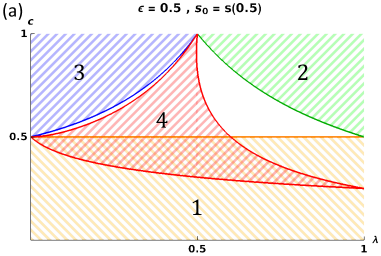
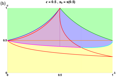
Refer to caption
Refer to caption
Figure 31: Regions 1-4 in (a) show the parameter ranges for which f1subscript𝑓1f_{1} through f4subscript𝑓4f_{4} are given by the saddle-point values in the first lines of (C.88)-(C.91). The resulting phase diagram for the logarithmic negativity is shown in (b). Different shaded regions correspond to distinct phases. All lines from (a), including those that do not correspond to phase transition lines of the logarithmic negativity, are also shown in (b) to make it easier to compare regions in the two figures.

Let us try to understand the phase diagram for the logarithmic negativity in terms of the parameters c=SA(eq)SA(eq)+SB(eq)𝑐subscriptsuperscript𝑆eq𝐴subscriptsuperscript𝑆eq𝐴subscriptsuperscript𝑆eq𝐵c=\frac{S^{\rm(eq)}_{A}}{S^{\rm(eq)}_{A}+S^{\rm(eq)}_{B}} and λ=SA1(eq)SA(eq)𝜆subscriptsuperscript𝑆eqsubscript𝐴1subscriptsuperscript𝑆eq𝐴\lambda=\frac{S^{\rm(eq)}_{A_{1}}}{S^{\rm(eq)}_{A}}. We first find the ranges of c,λ𝑐𝜆c,\lambda for which the different terms f1subscript𝑓1f_{1} through f4subscript𝑓4f_{4} are given by their saddle-point values (the first lines of equations (C.88)-(C.91)) in Fig. 31(a).

The parameter ranges where f2subscript𝑓2f_{2} and f3subscript𝑓3f_{3} take their saddle-point values are shown respectively by the green and blue regions in Fig. 31(a). In these regions, we find that f2subscript𝑓2f_{2} and f3subscript𝑓3f_{3} respectively are also larger than the other fisubscript𝑓𝑖f_{i}. Hence, in these regions the logarithmic negativity is given by

={S1/2,A1(eq)λ<12SA2(eq)λ>12casessubscriptsuperscript𝑆eq12subscript𝐴1𝜆12subscriptsuperscript𝑆eqsubscript𝐴2𝜆12{{\mathcal{E}}}=\begin{cases}S^{\rm(eq)}_{1/2,\,A_{1}}&\lambda<\frac{1}{2}\\ S^{\rm(eq)}_{A_{2}}&\lambda>\frac{1}{2}\end{cases} (C.93)

There is some intersection between the orange and red shaded regions in Fig. 31(a) where f1subscript𝑓1f_{1} and f4subscript𝑓4f_{4} respectively take their saddle point values. On comparing the first lines of (C.88) and (C.91), we find that the latter dominates for

12SA2eq+S1/3,A1eq12SA1eq12SBeq>0.12superscriptsubscript𝑆subscript𝐴2eqsuperscriptsubscript𝑆13subscript𝐴1eq12superscriptsubscript𝑆subscript𝐴1eq12subscriptsuperscript𝑆eq𝐵0\frac{1}{2}S_{A_{2}}^{\rm eq}+S_{1/3,A_{1}}^{\rm eq}-\frac{1}{2}S_{A_{1}}^{\rm eq}-\frac{1}{2}S^{\rm eq}_{B}>0\,. (C.94)

The condition (C.94) is shown with the pink line in Fig. 31(b). In the purple shaded region of Fig. 31(b), we find that f4subscript𝑓4f_{4} is also larger than f2subscript𝑓2f_{2} and f3subscript𝑓3f_{3}, and hence in this region the logarithmic negativity is given by

=12SA2eq+S1/3,A1eq12SA1eq12SBeq.12superscriptsubscript𝑆subscript𝐴2eqsuperscriptsubscript𝑆13subscript𝐴1eq12superscriptsubscript𝑆subscript𝐴1eq12subscriptsuperscript𝑆eq𝐵{{\mathcal{E}}}=\frac{1}{2}S_{A_{2}}^{\rm eq}+S_{1/3,A_{1}}^{\rm eq}-\frac{1}{2}S_{A_{1}}^{\rm eq}-\frac{1}{2}S^{\rm eq}_{B}\,. (C.95)

In the unshaded regions of Fig. 31 (a), none of the terms of (C.82) take their saddle-point values. In the left unshaded region of Fig. 31 (a), which is the same as the region shaded in red in Fig. 31 (b), we find that the dominant contribution is given by the second lines of f3subscript𝑓3f_{3} and f4subscript𝑓4f_{4}, which coincide with each other. In this region, the logarithmic negativity is given by

=SA2(eq)+VA1(s(θ3)s(ϵ))VBs(ϵ).subscriptsuperscript𝑆eqsubscript𝐴2subscript𝑉subscript𝐴1𝑠subscript𝜃3𝑠italic-ϵsubscript𝑉𝐵𝑠italic-ϵ{{\mathcal{E}}}=S^{\rm(eq)}_{A_{2}}+V_{A_{1}}(s(\theta_{3})-s(\epsilon))-V_{B}s(\epsilon)\,. (C.96)

In the blue shaded region of Fig. 31(b), which includes both the right unshaded region of Fig. 31(a) and part of the orange shaded region there, the dominant contribution is given by the second lines of f2subscript𝑓2f_{2} and f4subscript𝑓4f_{4}, which coincide. The logarithmic negativity here is given by

=VA1(2s(θ2)s(ϵ))VBs(ϵ).subscript𝑉subscript𝐴12𝑠subscript𝜃2𝑠italic-ϵsubscript𝑉𝐵𝑠italic-ϵ{{\mathcal{E}}}=V_{A_{1}}\,(2s(\theta_{2})-s(\epsilon))-V_{B}\,s(\epsilon)\,. (C.97)

Finally, in the yellow shaded region of Fig. 31(b), we have

=0.0{{\mathcal{E}}}=0\,. (C.98)

Each of the expressions (C.93), (C.95), (C.96), (C.97), (C.98) corresponds to a distinct phase, and there is a discontinuity in either the first or the second derivative of {{\mathcal{E}}} across each of the phase transition lines, as shown in Fig. 12.

Appendix D Maxima of functions of permutations at finite temperature

In this appendix, we use general properties of the function f(β)𝑓𝛽f(\beta) in any system to show that G(β,τ)𝐺𝛽𝜏G(\beta,\tau) (as defined in (4.64)) is maximized by τ=e𝜏𝑒\tau=e, while G(β,τ)+G(β,η1τ)𝐺𝛽𝜏𝐺𝛽superscript𝜂1𝜏G(\beta,\tau)+G(\beta,\eta^{-1}\tau) is maximized by both τ=e𝜏𝑒\tau=e and τ=η𝜏𝜂\tau=\eta.

Recall

G(β,τ)=i=1k(τ)f(ciβ)𝐺𝛽𝜏superscriptsubscript𝑖1𝑘𝜏𝑓subscript𝑐𝑖𝛽G(\beta,\tau)=\sum_{i=1}^{k(\tau)}f(c_{i}\beta) (D.1)

and

G(β,τ)+G(β,η1τ)=i=1k(τ)f(ciβ)+j=1k(η1τ)f(ajβ)𝐺𝛽𝜏𝐺𝛽superscript𝜂1𝜏superscriptsubscript𝑖1𝑘𝜏𝑓subscript𝑐𝑖𝛽superscriptsubscript𝑗1𝑘superscript𝜂1𝜏𝑓subscript𝑎𝑗𝛽G(\beta,\tau)+G(\beta,\eta^{-1}\tau)=\sum_{i=1}^{k(\tau)}f(c_{i}\beta)+\sum_{j=1}^{k(\eta^{-1}\tau)}f(a_{j}\beta) (D.2)

Both (D.1) and (D.2) are examples of sums of the form

P(S,m,{ci}):=i=1mf(ciβ),i=1mci=S,1cinformulae-sequenceassign𝑃𝑆𝑚subscript𝑐𝑖superscriptsubscript𝑖1𝑚𝑓subscript𝑐𝑖𝛽formulae-sequencesuperscriptsubscript𝑖1𝑚subscript𝑐𝑖𝑆1subscript𝑐𝑖𝑛P(S,m,\{c_{i}\}):=\sum_{i=1}^{m}f(c_{i}\beta),\quad\sum_{i=1}^{m}c_{i}=S,\quad 1\leq c_{i}\leq n (D.3)

where the m𝑚m numbers cisubscript𝑐𝑖c_{i} are all positive integers, and S𝑆S is either n𝑛n or 2n2𝑛2n. In fact, note that the above constraints together further restrict the range of the cisubscript𝑐𝑖c_{i}, to

1ciS(m1).1subscript𝑐𝑖𝑆𝑚11\leq c_{i}\leq S-(m-1)\,. (D.4)

To simplify the problem of finding τ𝜏\tau that maximize (D.1) and (D.2), we first ask: with the constraint in (D.4), what are the values of m,ci𝑚subscript𝑐𝑖m,c_{i} for which the function P(S,m,{ci})𝑃𝑆𝑚subscript𝑐𝑖P(S,m,\{c_{i}\}) is maximized?

We first fix m𝑚m, and see what set of m𝑚m numbers cisubscript𝑐𝑖c_{i} satisfying (D.4) maximizes P(S,m,{ci})𝑃𝑆𝑚subscript𝑐𝑖P(S,m,\{c_{i}\}). Note that since each cisubscript𝑐𝑖c_{i} lies between 1 and S(m1)𝑆𝑚1S-(m-1), it can be written as

ci=λ+(1λ)(S(m1))subscript𝑐𝑖𝜆1𝜆𝑆𝑚1c_{i}=\lambda+(1-\lambda)(S-(m-1)) (D.5)

where λ=Sm+1ciSm𝜆𝑆𝑚1subscript𝑐𝑖𝑆𝑚\lambda=\frac{S-m+1-c_{i}}{S-m} lies between 0 and 1. Then using (4.33) for each term in P(m,S,{ci})𝑃𝑚𝑆subscript𝑐𝑖P(m,S,\{c_{i}\}), we find

P(S,m,{ci})i=1m(Sm+1ciSmf(β)+ci1Smf((Sm+1)β))Q(m,S):=(m1)f(β)+f((Sm+1)β)𝑃𝑆𝑚subscript𝑐𝑖superscriptsubscript𝑖1𝑚𝑆𝑚1subscript𝑐𝑖𝑆𝑚𝑓𝛽subscript𝑐𝑖1𝑆𝑚𝑓𝑆𝑚1𝛽𝑄𝑚𝑆assign𝑚1𝑓𝛽𝑓𝑆𝑚1𝛽\begin{gathered}P(S,m,\{c_{i}\})\leq\sum_{i=1}^{m}\left(\frac{S-m+1-c_{i}}{S-m}f(\beta)+\frac{c_{i}-1}{S-m}f\left((S-m+1)\beta\right)\right)\\ \leq Q(m,S):=(m-1)f(\beta)+f\left((S-m+1)\beta\right)\end{gathered} (D.6)

Note further that Q(m,S)𝑄𝑚𝑆Q(m,S) is an increasing function of m𝑚m for both choices of S𝑆S, since (4.37) implies in particular that

f(β)βf((2nm+1)β)0,f(β)βf((nm+1)β)0.formulae-sequence𝑓𝛽𝛽superscript𝑓2𝑛𝑚1𝛽0𝑓𝛽𝛽superscript𝑓𝑛𝑚1𝛽0f(\beta)-\beta f^{\prime}((2n-m+1)\beta)\geq 0,\quad f(\beta)-\beta f^{\prime}((n-m+1)\beta)\geq 0. (D.7)

Hence, the following statements hold:

  1. 1.
    G(τ)=i=1k(τ)f(ciβ)nf(β)𝐺𝜏superscriptsubscript𝑖1𝑘𝜏𝑓subscript𝑐𝑖𝛽𝑛𝑓𝛽G(\tau)=\sum_{i=1}^{k(\tau)}f(c_{i}\beta)\leq nf(\beta) (D.8)

    This is because on comparing the definition of G(τ)𝐺𝜏G(\tau) to that of P(S,m,{ci})𝑃𝑆𝑚subscript𝑐𝑖P(S,m,\{c_{i}\}), we see that S=n𝑆𝑛S=n, and the maximum value of m𝑚m that can appear in G(τ)𝐺𝜏G(\tau) is n𝑛n. But the RHS of (D.8) is the value of the LHS for τ=e𝜏𝑒\tau=e, so G(τ)=i=1k(τ)f(ciβ)𝐺𝜏superscriptsubscript𝑖1𝑘𝜏𝑓subscript𝑐𝑖𝛽G(\tau)=\sum_{i=1}^{k(\tau)}f(c_{i}\beta) is maximized by τ=e𝜏𝑒\tau=e.

  2. 2.
    G(τ)+G(ητ1)=i=1k(τ)f(ciβ)+j=1k(ητ1)f(ajβ)nf(β)+f(nβ)𝐺𝜏𝐺𝜂superscript𝜏1superscriptsubscript𝑖1𝑘𝜏𝑓subscript𝑐𝑖𝛽superscriptsubscript𝑗1𝑘𝜂superscript𝜏1𝑓subscript𝑎𝑗𝛽𝑛𝑓𝛽𝑓𝑛𝛽G(\tau)+G(\eta\tau^{-1})=\sum_{i=1}^{k(\tau)}f(c_{i}\beta)+\sum_{j=1}^{k(\eta\tau^{-1})}f(a_{j}\beta)\leq nf(\beta)+f(n\beta) (D.9)

    This follows since the maximum number of terms in this full expression is n+1𝑛1n+1 since k(τ)+k(ητ1)n+1𝑘𝜏𝑘𝜂superscript𝜏1𝑛1k(\tau)+k(\eta\tau^{-1})\leq n+1, and here S=2n𝑆2𝑛S=2n. The RHS is the value of the LHS for τ=e𝜏𝑒\tau=e and τ=η𝜏𝜂\tau=\eta, so G(τ)+G(ητ1)𝐺𝜏𝐺𝜂superscript𝜏1G(\tau)+G(\eta\tau^{-1}) is maximized by both.

Appendix E 𝒵n(PT)superscriptsubscript𝒵𝑛PT{\mathcal{Z}}_{n}^{\rm(PT)} in the microcanonical ensemble with energy conservation in AB𝐴𝐵AB

Let us now consider the equilibrium approximation with αsubscript𝛼{{\mathcal{I}}}_{{\alpha}} as in (4.75). Unlike in the simpler example in the previous subsection, we are not able to compute the logarithmic negativity through the resolvent in this example. However, we can find the phase diagram for 𝒵n(PT)superscriptsubscript𝒵𝑛PT{\mathcal{Z}}_{n}^{\rm(PT)} and the Renyi negativities, which have the same qualitative features as those for the canonical example and the simple example of the previous subsection.

Let us assume that like in other universality classes, the dominant contribution is always given by one out of e𝑒e, η𝜂\eta, η1superscript𝜂1\eta^{-1}, and τESsubscript𝜏𝐸𝑆\tau_{ES}. Let us try to understand the contributions that we get from each of these permutations. In each case, we can use diagrams similar to Fig. 27, now taking into account energy conservation between all three subsystems A1subscript𝐴1A_{1}, A2subscript𝐴2A_{2}, and B𝐵B. We then find:

  1. 1.
    𝒵n(PT)(e)=1NEnE1,E2dE1A1dE2A2(dEE1E2B)nsuperscriptsubscript𝒵𝑛PT𝑒1superscriptsubscript𝑁𝐸𝑛subscriptsubscript𝐸1subscript𝐸2subscriptsuperscript𝑑subscript𝐴1subscript𝐸1subscriptsuperscript𝑑subscript𝐴2subscript𝐸2superscriptsubscriptsuperscript𝑑𝐵𝐸subscript𝐸1subscript𝐸2𝑛\begin{gathered}{\mathcal{Z}}_{n}^{\rm(PT)}(e)=\frac{1}{N_{E}^{n}}\sum_{E_{1},E_{2}}d^{A_{1}}_{E_{1}}d^{A_{2}}_{E_{2}}(d^{B}_{E-E_{1}-E_{2}})^{n}\end{gathered} (E.1)

    Expressing each density of states in terms of the corresponding entropy density (e.g. dE1A1=exp(VA1s(E1VA1))subscriptsuperscript𝑑subscript𝐴1subscript𝐸1subscript𝑉subscript𝐴1𝑠subscript𝐸1subscript𝑉subscript𝐴1d^{A_{1}}_{E_{1}}=\exp({V_{A_{1}}s(\frac{E_{1}}{V_{A_{1}}})}) ), we find that the saddle-point equations for the energy densities ϵ1=E1VA1subscriptitalic-ϵ1subscript𝐸1subscript𝑉subscript𝐴1\epsilon_{1}=\frac{E_{1}}{V_{A_{1}}} and ϵ1=E2VA2subscriptitalic-ϵ1subscript𝐸2subscript𝑉subscript𝐴2\epsilon_{1}=\frac{E_{2}}{V_{A_{2}}} are

    s(ϵ1)=ns(VϵVA1ϵ1VA2ϵ2VB)superscript𝑠subscriptitalic-ϵ1𝑛superscript𝑠𝑉italic-ϵsubscript𝑉subscript𝐴1subscriptitalic-ϵ1subscript𝑉subscript𝐴2subscriptitalic-ϵ2subscript𝑉𝐵\displaystyle s^{\prime}(\epsilon_{1})=ns^{\prime}\left(\frac{V\epsilon-V_{A_{1}}\epsilon_{1}-V_{A_{2}}\epsilon_{2}}{V_{B}}\right) (E.2)
    s(ϵ2)=ns(VϵVA1ϵ1VA2ϵ2VB)superscript𝑠subscriptitalic-ϵ2𝑛superscript𝑠𝑉italic-ϵsubscript𝑉subscript𝐴1subscriptitalic-ϵ1subscript𝑉subscript𝐴2subscriptitalic-ϵ2subscript𝑉𝐵\displaystyle s^{\prime}(\epsilon_{2})=ns^{\prime}\left(\frac{V\epsilon-V_{A_{1}}\epsilon_{1}-V_{A_{2}}\epsilon_{2}}{V_{B}}\right) (E.3)

    where ϵ=EVitalic-ϵ𝐸𝑉\epsilon=\frac{E}{V}. Since the RHS of (E.2) and (E.3) is the same, we can assume that ϵ1=ϵ2=ϵesubscriptitalic-ϵ1subscriptitalic-ϵ2subscriptitalic-ϵ𝑒\epsilon_{1}=\epsilon_{2}=\epsilon_{e}, and solve

    s(ϵe)=ns(VϵVAϵeVB)superscript𝑠subscriptitalic-ϵ𝑒𝑛superscript𝑠𝑉italic-ϵsubscript𝑉𝐴subscriptitalic-ϵ𝑒subscript𝑉𝐵s^{\prime}(\epsilon_{e})=ns^{\prime}\left(\frac{V\epsilon-V_{A}\epsilon_{e}}{V_{B}}\right) (E.4)

    We therefore find

    𝒵n(PT)(e)eVAs(ϵe)+nVBs(VϵVAϵeVB)Vns(ϵ).superscriptsubscript𝒵𝑛PT𝑒superscript𝑒subscript𝑉𝐴𝑠subscriptitalic-ϵ𝑒𝑛subscript𝑉𝐵𝑠𝑉italic-ϵsubscript𝑉𝐴subscriptitalic-ϵ𝑒subscript𝑉𝐵𝑉𝑛𝑠italic-ϵ{\mathcal{Z}}_{n}^{\rm(PT)}(e)\approx e^{V_{A}s(\epsilon_{e})+nV_{B}s\left(\frac{V\epsilon-V_{A}\epsilon_{e}}{V_{B}}\right)-Vns(\epsilon)}\,. (E.5)

    Taking the n1𝑛1n\rightarrow 1 limit of (E.4) and (E.5) gives

    =0.0{{\mathcal{E}}}=0\,. (E.6)
  2. 2.
    𝒵n(PT)(η)=1NEnEB,E2,E2dEBBdE2A2dE2A2(dEE2EBA1)n2(dEE2EBA1)n2superscriptsubscript𝒵𝑛PT𝜂1superscriptsubscript𝑁𝐸𝑛subscriptsubscript𝐸𝐵subscript𝐸2subscriptsuperscript𝐸2subscriptsuperscript𝑑𝐵subscript𝐸𝐵subscriptsuperscript𝑑subscript𝐴2subscript𝐸2subscriptsuperscript𝑑subscript𝐴2subscriptsuperscript𝐸2superscriptsubscriptsuperscript𝑑subscript𝐴1𝐸subscript𝐸2subscript𝐸𝐵𝑛2superscriptsubscriptsuperscript𝑑subscript𝐴1𝐸subscriptsuperscript𝐸2subscript𝐸𝐵𝑛2\begin{gathered}{\mathcal{Z}}_{n}^{\rm(PT)}(\eta)=\frac{1}{N_{E}^{n}}\sum_{E_{B},E_{2},E^{\prime}_{2}}d^{B}_{E_{B}}\,d^{A_{2}}_{E_{2}}\,d^{A_{2}}_{E^{\prime}_{2}}\,(d^{A_{1}}_{E-E_{2}-E_{B}})^{\frac{n}{2}}\,(d^{A_{1}}_{E-E^{\prime}_{2}-E_{B}})^{\frac{n}{2}}\\ \end{gathered} (E.7)

    The saddle-point equations for the energy densities ϵB=EBVBsubscriptitalic-ϵ𝐵subscript𝐸𝐵subscript𝑉𝐵\epsilon_{B}=\frac{E_{B}}{V_{B}}, ϵ2=E2VA2subscriptitalic-ϵ2subscript𝐸2subscript𝑉subscript𝐴2\epsilon_{2}=\frac{E_{2}}{V_{A_{2}}}, and ϵ2=E2VA2subscriptsuperscriptitalic-ϵ2subscriptsuperscript𝐸2subscript𝑉subscript𝐴2\epsilon^{\prime}_{2}=\frac{E^{\prime}_{2}}{V_{A_{2}}} are

    s(ϵB)n2s(ϵVVA2ϵ2VBϵBVA1)n2s(ϵVVA2ϵ2VBϵBVA1)=0superscript𝑠subscriptitalic-ϵ𝐵𝑛2superscript𝑠italic-ϵ𝑉subscript𝑉subscript𝐴2subscriptitalic-ϵ2subscript𝑉𝐵subscriptitalic-ϵ𝐵subscript𝑉subscript𝐴1𝑛2superscript𝑠italic-ϵ𝑉subscript𝑉subscript𝐴2subscriptsuperscriptitalic-ϵ2subscript𝑉𝐵subscriptitalic-ϵ𝐵subscript𝑉subscript𝐴10\displaystyle s^{\prime}(\epsilon_{B})-\frac{n}{2}s^{\prime}\left(\frac{\epsilon V-V_{A_{2}}\epsilon_{2}-V_{B}\epsilon_{B}}{V_{A_{1}}}\right)-\frac{n}{2}s^{\prime}\left(\frac{\epsilon V-V_{A_{2}}\epsilon^{\prime}_{2}-V_{B}\epsilon_{B}}{V_{A_{1}}}\right)=0 (E.8)
    s(ϵ2)n2s(ϵVVA2ϵ2VBϵBVA1)=0superscript𝑠subscriptitalic-ϵ2𝑛2superscript𝑠italic-ϵ𝑉subscript𝑉subscript𝐴2subscriptitalic-ϵ2subscript𝑉𝐵subscriptitalic-ϵ𝐵subscript𝑉subscript𝐴10\displaystyle s^{\prime}(\epsilon_{2})-\frac{n}{2}s^{\prime}\left(\frac{\epsilon V-V_{A_{2}}\epsilon_{2}-V_{B}\epsilon_{B}}{V_{A_{1}}}\right)=0 (E.9)
    s(ϵ2)n2s(ϵVVA2ϵ2VBϵBVA1)=0superscript𝑠subscriptsuperscriptitalic-ϵ2𝑛2superscript𝑠italic-ϵ𝑉subscript𝑉subscript𝐴2subscriptsuperscriptitalic-ϵ2subscript𝑉𝐵subscriptitalic-ϵ𝐵subscript𝑉subscript𝐴10\displaystyle s^{\prime}(\epsilon^{\prime}_{2})-\frac{n}{2}s^{\prime}\left(\frac{\epsilon V-V_{A_{2}}\epsilon^{\prime}_{2}-V_{B}\epsilon_{B}}{V_{A_{1}}}\right)=0 (E.10)

    Since the system of equations is unchanged on exchanging ϵ2subscriptitalic-ϵ2\epsilon_{2} with ϵ2subscriptsuperscriptitalic-ϵ2\epsilon^{\prime}_{2} everywhere, the solutions for both variables will be the same. Hence, we can simplify the equations by setting ϵ2=ϵ2=ϵ2ηsubscriptitalic-ϵ2subscriptsuperscriptitalic-ϵ2superscriptsubscriptitalic-ϵ2𝜂\epsilon_{2}=\epsilon^{\prime}_{2}=\epsilon_{2}^{\eta}. Then we must solve the following two equations for ϵ2ηsuperscriptsubscriptitalic-ϵ2𝜂\epsilon_{2}^{\eta} and ϵBηsuperscriptsubscriptitalic-ϵ𝐵𝜂\epsilon_{B}^{\eta}:

    s(ϵBη)ns(VϵVA2ϵ2ηVBϵBηVA1)=0superscript𝑠superscriptsubscriptitalic-ϵ𝐵𝜂𝑛superscript𝑠𝑉italic-ϵsubscript𝑉subscript𝐴2superscriptsubscriptitalic-ϵ2𝜂subscript𝑉𝐵superscriptsubscriptitalic-ϵ𝐵𝜂subscript𝑉subscript𝐴10\displaystyle s^{\prime}(\epsilon_{B}^{\eta})-ns^{\prime}\left(\frac{V\epsilon-V_{A_{2}}\epsilon_{2}^{\eta}-V_{B}\epsilon_{B}^{\eta}}{V_{A_{1}}}\right)=0 (E.11)
    s(ϵ2η)n2s(VϵVA2ϵ2ηVBϵBηVA1)=0superscript𝑠superscriptsubscriptitalic-ϵ2𝜂𝑛2superscript𝑠𝑉italic-ϵsubscript𝑉subscript𝐴2superscriptsubscriptitalic-ϵ2𝜂subscript𝑉𝐵superscriptsubscriptitalic-ϵ𝐵𝜂subscript𝑉subscript𝐴10\displaystyle s^{\prime}(\epsilon_{2}^{\eta})-\frac{n}{2}s^{\prime}\left(\frac{V\epsilon-V_{A_{2}}\epsilon_{2}^{\eta}-V_{B}\epsilon_{B}^{\eta}}{V_{A_{1}}}\right)=0 (E.12)

    to find

    𝒵n(PT)(η)exp(VBs(ϵBη)+2VA2s(ϵ2η)+nVA1s(VϵVA2ϵ2ηVBϵBηVA1)nVs(ϵ))superscriptsubscript𝒵𝑛PT𝜂subscript𝑉𝐵𝑠superscriptsubscriptitalic-ϵ𝐵𝜂2subscript𝑉subscript𝐴2𝑠superscriptsubscriptitalic-ϵ2𝜂𝑛subscript𝑉subscript𝐴1𝑠𝑉italic-ϵsubscript𝑉subscript𝐴2superscriptsubscriptitalic-ϵ2𝜂subscript𝑉𝐵superscriptsubscriptitalic-ϵ𝐵𝜂subscript𝑉subscript𝐴1𝑛𝑉𝑠italic-ϵ{\mathcal{Z}}_{n}^{\rm(PT)}(\eta)\approx\exp(V_{B}s(\epsilon_{B}^{\eta})+2V_{A_{2}}s(\epsilon_{2}^{\eta})+nV_{A_{1}}s\left(\frac{V-\epsilon V_{A_{2}}\epsilon_{2}^{\eta}-V_{B}\epsilon_{B}^{\eta}}{V_{A_{1}}}\right)-nVs(\epsilon)) (E.13)

    For general forms of s(ϵ)𝑠italic-ϵs(\epsilon), there is no relation between (E.13) for general n𝑛n and the Renyi entropies of ρ(eq)superscript𝜌eq\rho^{\rm(eq)}. But for n=1𝑛1n=1, (E.11), (E.12) and (E.13) simplify such that we have

    =S12,A2(eq)subscriptsuperscript𝑆eq12subscript𝐴2{{\mathcal{E}}}=S^{\rm(eq)}_{\frac{1}{2},A_{2}} (E.14)

    Similarly, taking the n1𝑛1n\rightarrow 1 limit of 𝒵n(PT)(η1)superscriptsubscript𝒵𝑛PTsuperscript𝜂1{\mathcal{Z}}_{n}^{\rm(PT)}(\eta^{-1}), we find

    =S12,A1(eq).subscriptsuperscript𝑆eq12subscript𝐴1{{\mathcal{E}}}=S^{\rm(eq)}_{\frac{1}{2},A_{1}}\,. (E.15)
  3. 3.

    Now consider the contribution from τESsubscript𝜏𝐸𝑆\tau_{ES}:

    𝒵n(PT)(τES)=1NEnE1,E1,EB1,EB2,,EBn/2(j=1n/2dEBjB)dEE1EB1A2(j=1n/2dEE1EBjA2)×dE1A1dE1A1(j=2n/2dE1+EB1EBjA1)superscriptsubscript𝒵𝑛PTsubscript𝜏𝐸𝑆1superscriptsubscript𝑁𝐸𝑛subscriptsubscript𝐸1subscriptsuperscript𝐸1superscriptsubscript𝐸𝐵1superscriptsubscript𝐸𝐵2superscriptsubscript𝐸𝐵𝑛2superscriptsubscriptproduct𝑗1𝑛2subscriptsuperscript𝑑𝐵superscriptsubscript𝐸𝐵𝑗subscriptsuperscript𝑑subscript𝐴2𝐸subscript𝐸1superscriptsubscript𝐸𝐵1superscriptsubscriptproduct𝑗1𝑛2subscriptsuperscript𝑑subscript𝐴2𝐸subscriptsuperscript𝐸1superscriptsubscript𝐸𝐵𝑗subscriptsuperscript𝑑subscript𝐴1subscriptsuperscript𝐸1subscriptsuperscript𝑑subscript𝐴1subscript𝐸1superscriptsubscriptproduct𝑗2𝑛2subscriptsuperscript𝑑subscript𝐴1subscript𝐸1superscriptsubscript𝐸𝐵1superscriptsubscript𝐸𝐵𝑗\begin{gathered}{\mathcal{Z}}_{n}^{\rm(PT)}(\tau_{ES})=\frac{1}{N_{E}^{n}}\sum_{\begin{subarray}{c}E_{1},E^{\prime}_{1},E_{B}^{1},\\ E_{B}^{2},...,E_{B}^{n/2}\end{subarray}}\left(\prod_{j=1}^{n/2}d^{B}_{E_{B}^{j}}\right)~{}d^{A_{2}}_{E-E_{1}-E_{B}^{1}}\left(\prod_{j=1}^{n/2}d^{A_{2}}_{E-E^{\prime}_{1}-E_{B}^{j}}\right)\\ ~{}\times d^{A_{1}}_{E^{\prime}_{1}}d^{A_{1}}_{E_{1}}\left(\prod_{j=2}^{n/2}d^{A_{1}}_{E_{1}+E_{B}^{1}-E_{B}^{j}}\right)\end{gathered} (E.16)

    The n+2𝑛2n+2 saddle point equations are

    s(ϵB1)s(VϵVA1ϵ1VBϵB1VA2)s(VϵVA1ϵ1VBϵB1VA2)superscript𝑠superscriptsubscriptitalic-ϵ𝐵1superscript𝑠𝑉italic-ϵsubscript𝑉subscript𝐴1subscriptitalic-ϵ1subscript𝑉𝐵superscriptsubscriptitalic-ϵ𝐵1subscript𝑉subscript𝐴2superscript𝑠𝑉italic-ϵsubscript𝑉subscript𝐴1subscriptsuperscriptitalic-ϵ1subscript𝑉𝐵superscriptsubscriptitalic-ϵ𝐵1subscript𝑉subscript𝐴2\displaystyle s^{\prime}(\epsilon_{B}^{1})-s^{\prime}\left(\frac{V\epsilon-V_{A_{1}}\epsilon_{1}-V_{B}\epsilon_{B}^{1}}{V_{A_{2}}}\right)-s^{\prime}\left(\frac{V\epsilon-V_{A_{1}}\epsilon^{\prime}_{1}-V_{B}\epsilon_{B}^{1}}{V_{A_{2}}}\right)
    +j=2n/2s(ϵ1+VBVA1(ϵB1ϵBj))=0superscriptsubscript𝑗2𝑛2superscript𝑠subscriptitalic-ϵ1subscript𝑉𝐵subscript𝑉subscript𝐴1superscriptsubscriptitalic-ϵ𝐵1superscriptsubscriptitalic-ϵ𝐵𝑗0\displaystyle+\sum_{j=2}^{n/2}s^{\prime}\left(\epsilon_{1}+\frac{V_{B}}{V_{A_{1}}}(\epsilon_{B}^{1}-\epsilon_{B}^{j})\right)=0 (E.17)
    s(ϵ1)s(ϵVA1ϵ1VBϵB1VA2)+j=2n/2s(ϵ1+VBVA2(ϵB1ϵBj))=0superscript𝑠subscriptitalic-ϵ1superscript𝑠italic-ϵsubscript𝑉subscript𝐴1subscriptitalic-ϵ1subscript𝑉𝐵superscriptsubscriptitalic-ϵ𝐵1subscript𝑉subscript𝐴2superscriptsubscript𝑗2𝑛2superscript𝑠subscriptitalic-ϵ1subscript𝑉𝐵subscript𝑉subscript𝐴2superscriptsubscriptitalic-ϵ𝐵1superscriptsubscriptitalic-ϵ𝐵𝑗0\displaystyle s^{\prime}(\epsilon_{1})-s^{\prime}\left(\frac{\epsilon-V_{A_{1}}\epsilon_{1}-V_{B}\epsilon_{B}^{1}}{V_{A_{2}}}\right)+\sum_{j=2}^{n/2}s^{\prime}\left(\epsilon_{1}+\frac{V_{B}}{V_{A_{2}}}(\epsilon_{B}^{1}-\epsilon_{B}^{j})\right)=0 (E.18)
    s(ϵ1)j=1n/2s(ϵVVA1ϵ1VBϵBjVA2)=0superscript𝑠subscriptsuperscriptitalic-ϵ1superscriptsubscript𝑗1𝑛2superscript𝑠italic-ϵ𝑉subscript𝑉subscript𝐴1subscriptsuperscriptitalic-ϵ1subscript𝑉𝐵superscriptsubscriptitalic-ϵ𝐵𝑗subscript𝑉subscript𝐴20\displaystyle s^{\prime}(\epsilon^{\prime}_{1})-\sum_{j=1}^{n/2}s^{\prime}\left(\frac{\epsilon V-V_{A_{1}}\epsilon^{\prime}_{1}-V_{B}\epsilon_{B}^{j}}{V_{A_{2}}}\right)=0 (E.19)
    s(ϵBj)s(VϵVA1ϵ1VBϵBjVA2)s(ϵ1+VBVA1(ϵB1ϵBj))=0,j=2,,nformulae-sequencesuperscript𝑠superscriptsubscriptitalic-ϵ𝐵𝑗superscript𝑠𝑉italic-ϵsubscript𝑉subscript𝐴1subscriptsuperscriptitalic-ϵ1subscript𝑉𝐵superscriptsubscriptitalic-ϵ𝐵𝑗subscript𝑉subscript𝐴2superscript𝑠subscriptitalic-ϵ1subscript𝑉𝐵subscript𝑉subscript𝐴1superscriptsubscriptitalic-ϵ𝐵1superscriptsubscriptitalic-ϵ𝐵𝑗0𝑗2𝑛\displaystyle s^{\prime}(\epsilon_{B}^{j})-s^{\prime}\left(\frac{V\epsilon-V_{A_{1}}\epsilon^{\prime}_{1}-V_{B}\epsilon_{B}^{j}}{V_{A_{2}}}\right)-s^{\prime}\left(\epsilon_{1}+\frac{V_{B}}{V_{A_{1}}}(\epsilon_{B}^{1}-\epsilon_{B}^{j})\right)=0,\quad j=2,...,n (E.20)

    Note that this set of equations is invariant under permuting the ϵBjsuperscriptsubscriptitalic-ϵ𝐵𝑗\epsilon_{B}^{j} from j=2𝑗2j=2 to n𝑛n. We can therefore assume that these variables have the same solution, so that we have a simpler set of four equations for any n𝑛n:

    s(ϵB1)s(VϵVA1ϵ1VBϵB1VA2)s(VϵVA1ϵ1VBϵB1VA2)superscript𝑠superscriptsubscriptitalic-ϵ𝐵1superscript𝑠𝑉italic-ϵsubscript𝑉subscript𝐴1subscriptitalic-ϵ1subscript𝑉𝐵superscriptsubscriptitalic-ϵ𝐵1subscript𝑉subscript𝐴2superscript𝑠𝑉italic-ϵsubscript𝑉subscript𝐴1subscriptsuperscriptitalic-ϵ1subscript𝑉𝐵superscriptsubscriptitalic-ϵ𝐵1subscript𝑉subscript𝐴2\displaystyle s^{\prime}(\epsilon_{B}^{1})-s^{\prime}\left(\frac{V\epsilon-V_{A_{1}}\epsilon_{1}-V_{B}\epsilon_{B}^{1}}{V_{A_{2}}}\right)-s^{\prime}\left(\frac{V\epsilon-V_{A_{1}}\epsilon^{\prime}_{1}-V_{B}\epsilon_{B}^{1}}{V_{A_{2}}}\right)
    +(n21)s(ϵ1+VBVA1(ϵB1ϵBj))=0𝑛21superscript𝑠subscriptitalic-ϵ1subscript𝑉𝐵subscript𝑉subscript𝐴1superscriptsubscriptitalic-ϵ𝐵1superscriptsubscriptitalic-ϵ𝐵𝑗0\displaystyle+(\frac{n}{2}-1)s^{\prime}\left(\epsilon_{1}+\frac{V_{B}}{V_{A_{1}}}(\epsilon_{B}^{1}-\epsilon_{B}^{j})\right)=0 (E.21)
    s(ϵ1)s(VϵVA1ϵ1VBϵB1VA2)+(n21)s(ϵ1+VBVA1(ϵB1ϵBj))=0superscript𝑠subscriptitalic-ϵ1superscript𝑠𝑉italic-ϵsubscript𝑉subscript𝐴1subscriptitalic-ϵ1subscript𝑉𝐵superscriptsubscriptitalic-ϵ𝐵1subscript𝑉subscript𝐴2𝑛21superscript𝑠subscriptitalic-ϵ1subscript𝑉𝐵subscript𝑉subscript𝐴1superscriptsubscriptitalic-ϵ𝐵1superscriptsubscriptitalic-ϵ𝐵𝑗0\displaystyle s^{\prime}(\epsilon_{1})-s^{\prime}\left(\frac{V\epsilon-V_{A_{1}}\epsilon_{1}-V_{B}\epsilon_{B}^{1}}{V_{A_{2}}}\right)+(\frac{n}{2}-1)s^{\prime}\left(\epsilon_{1}+\frac{V_{B}}{V_{A_{1}}}(\epsilon_{B}^{1}-\epsilon_{B}^{j})\right)=0 (E.22)
    s(ϵ1)s(VϵVA1ϵ1VBϵB1VA2)(n21)s(VϵVA1ϵ1VBϵBjVA2)=0superscript𝑠subscriptsuperscriptitalic-ϵ1superscript𝑠𝑉italic-ϵsubscript𝑉subscript𝐴1subscriptsuperscriptitalic-ϵ1subscript𝑉𝐵superscriptsubscriptitalic-ϵ𝐵1subscript𝑉subscript𝐴2𝑛21superscript𝑠𝑉italic-ϵsubscript𝑉subscript𝐴1subscriptsuperscriptitalic-ϵ1subscript𝑉𝐵superscriptsubscriptitalic-ϵ𝐵𝑗subscript𝑉subscript𝐴20\displaystyle s^{\prime}(\epsilon^{\prime}_{1})-s^{\prime}\left(\frac{V\epsilon-V_{A_{1}}\epsilon^{\prime}_{1}-V_{B}\epsilon_{B}^{1}}{V_{A_{2}}}\right)-(\frac{n}{2}-1)s^{\prime}\left(\frac{V\epsilon-V_{A_{1}}\epsilon^{\prime}_{1}-V_{B}\epsilon_{B}^{j}}{V_{A_{2}}}\right)=0 (E.23)
    s(ϵBj)s(VϵVA1ϵ1VBϵBjVA2)s(ϵ1+VBVA1(ϵB1ϵBj))=0,j=2,,nformulae-sequencesuperscript𝑠superscriptsubscriptitalic-ϵ𝐵𝑗superscript𝑠𝑉italic-ϵsubscript𝑉subscript𝐴1subscriptsuperscriptitalic-ϵ1subscript𝑉𝐵superscriptsubscriptitalic-ϵ𝐵𝑗subscript𝑉subscript𝐴2superscript𝑠subscriptitalic-ϵ1subscript𝑉𝐵subscript𝑉subscript𝐴1superscriptsubscriptitalic-ϵ𝐵1superscriptsubscriptitalic-ϵ𝐵𝑗0𝑗2𝑛\displaystyle s^{\prime}(\epsilon_{B}^{j})-s^{\prime}\left(\frac{V\epsilon-V_{A_{1}}\epsilon^{\prime}_{1}-V_{B}\epsilon_{B}^{j}}{V_{A_{2}}}\right)-s^{\prime}\left(\epsilon_{1}+\frac{V_{B}}{V_{A_{1}}}(\epsilon_{B}^{1}-\epsilon_{B}^{j})\right)=0,\quad j=2,...,n (E.24)

    In terms of the solution {ϵ¯1,ϵ¯1,ϵ¯Bj,ϵ¯B1}subscript¯italic-ϵ1subscriptsuperscript¯italic-ϵ1superscriptsubscript¯italic-ϵ𝐵𝑗superscriptsubscript¯italic-ϵ𝐵1\{\bar{\epsilon}_{1},\bar{\epsilon}^{\prime}_{1},\bar{\epsilon}_{B}^{j},\bar{\epsilon}_{B}^{1}\} to these equations, we can write

    𝒵n(PT)(τES)exp(VB(n21)s(ϵ¯Bj)+VBs(ϵ¯B1)+VA2s(VϵVA1ϵ¯1VBϵ¯B1VA2)+VA2(n21)s(VϵVA1ϵ¯1VBϵ¯BjVA2)+VA2s(VϵVA1ϵ¯1VBϵ¯B1VA2)+VA1s(ϵ¯1)+VA1s(ϵ¯1)+VA1(n21)s(ϵ¯1+VBVA1(ϵ¯B1ϵ¯Bj))Vns(ϵ))superscriptsubscript𝒵𝑛PTsubscript𝜏ESsubscript𝑉𝐵𝑛21𝑠superscriptsubscript¯italic-ϵ𝐵𝑗subscript𝑉𝐵𝑠superscriptsubscript¯italic-ϵ𝐵1subscript𝑉subscript𝐴2𝑠𝑉italic-ϵsubscript𝑉subscript𝐴1subscript¯italic-ϵ1subscript𝑉𝐵superscriptsubscript¯italic-ϵ𝐵1subscript𝑉subscript𝐴2subscript𝑉subscript𝐴2𝑛21𝑠𝑉italic-ϵsubscript𝑉subscript𝐴1subscriptsuperscript¯italic-ϵ1subscript𝑉𝐵superscriptsubscript¯italic-ϵ𝐵𝑗subscript𝑉subscript𝐴2subscript𝑉subscript𝐴2𝑠𝑉italic-ϵsubscript𝑉subscript𝐴1subscriptsuperscript¯italic-ϵ1subscript𝑉𝐵superscriptsubscript¯italic-ϵ𝐵1subscript𝑉subscript𝐴2subscript𝑉subscript𝐴1𝑠subscriptsuperscript¯italic-ϵ1subscript𝑉subscript𝐴1𝑠subscript¯italic-ϵ1subscript𝑉subscript𝐴1𝑛21𝑠subscript¯italic-ϵ1subscript𝑉𝐵subscript𝑉subscript𝐴1superscriptsubscript¯italic-ϵ𝐵1superscriptsubscript¯italic-ϵ𝐵𝑗𝑉𝑛𝑠italic-ϵ\begin{gathered}{\mathcal{Z}}_{n}^{\rm(PT)}(\tau_{\rm ES})\approx\exp(V_{B}(\frac{n}{2}-1)s(\bar{\epsilon}_{B}^{j})+V_{B}s(\bar{\epsilon}_{B}^{1})+V_{A_{2}}s(\frac{V\epsilon-V_{A_{1}}\bar{\epsilon}_{1}-V_{B}\bar{\epsilon}_{B}^{1}}{V_{A_{2}}})\\ +V_{A_{2}}(\frac{n}{2}-1)s\left(\frac{V\epsilon-V_{A_{1}}\bar{\epsilon}^{\prime}_{1}-V_{B}\bar{\epsilon}_{B}^{j}}{V_{A_{2}}}\right)+V_{A_{2}}s\left(\frac{V\epsilon-V_{A_{1}}\bar{\epsilon}^{\prime}_{1}-V_{B}\bar{\epsilon}_{B}^{1}}{V_{A_{2}}}\right)\\ +V_{A_{1}}s(\bar{\epsilon}^{\prime}_{1})+V_{A_{1}}s(\bar{\epsilon}_{1})+V_{A_{1}}(\frac{n}{2}-1)s\left(\bar{\epsilon}_{1}+\frac{V_{B}}{V_{A_{1}}}(\bar{\epsilon}_{B}^{1}-\bar{\epsilon}_{B}^{j})\right)-Vns(\epsilon))\end{gathered} (E.25)

    In this case, it is not clear how to take the n1𝑛1n\rightarrow 1 limit, so we do not get simple expressions for {{\mathcal{E}}} like in the other phases.

(E.21)-(E.24) are difficult to solve for general forms of s(ϵ)𝑠italic-ϵs(\epsilon), so that it is difficult to find even the phase diagram for 𝒵n(PT)superscriptsubscript𝒵𝑛PT{\mathcal{Z}}_{n}^{\rm(PT)} for general s(ϵ)𝑠italic-ϵs(\epsilon). As one simple example, let us consider the Gaussian form of the entropy density

s(ϵ)=log212ϵ2𝑠italic-ϵ212superscriptitalic-ϵ2s(\epsilon)=\log 2-\frac{1}{2}\epsilon^{2} (E.26)

This form is an approximation for the entropy density of discrete systems, such as those with g(β)𝑔𝛽g(\beta) given by (4.58), close to ϵ=0italic-ϵ0\epsilon=0. The phase diagrams for 𝒵n(PT)superscriptsubscript𝒵𝑛PT{\mathcal{Z}}_{n}^{\rm(PT)} with this form of s(ϵ)𝑠italic-ϵs(\epsilon) for the n=4𝑛4n=4 and n=6𝑛6n=6 are shown in Fig. 32.

Refer to caption
Refer to caption
Figure 32: Phase transition lines for the n=4,6𝑛46n=4,6 Renyi negativities in the homogeneous microcanonical ensemble case, with s(ϵ)𝑠italic-ϵs(\epsilon) given by (E.26).

Appendix F Finite temperature Page curve in inhomogeneous systems

In this appendix, we show that the expression (2.49) for the von Neumann entropy SAsubscript𝑆𝐴S_{A} in an equilibrated pure state holds in two examples where AB𝐴𝐵AB is inhomogeneous. In such examples, the Page transition in different Renyi entropies Sn,Asubscript𝑆𝑛𝐴S_{n,A} takes place at different values of c=SA(eq)SA(eq)+SB(eq)𝑐subscriptsuperscript𝑆eq𝐴subscriptsuperscript𝑆eq𝐴subscriptsuperscript𝑆eq𝐵c=\frac{S^{\rm(eq)}_{A}}{S^{\rm(eq)}_{A}+S^{\rm(eq)}_{B}}. Hence, we cannot a priori deduce the form of the von Neumann entropy by analytic continuation, and instead we must use the resolvent for the reduced density matrix ρAsubscript𝜌𝐴\rho_{A}, defined in (2.13).

F.1 Canonical ensemble with A𝐴A at infinite temperature and A¯¯𝐴\bar{A} at finite temperature

Consider the effective identity operator

α=𝟏AeβHB,subscript𝛼tensor-productsubscript1𝐴superscript𝑒𝛽subscript𝐻𝐵{{\mathcal{I}}}_{{\alpha}}=\mathbf{1}_{A}\otimes e^{-\beta H_{B}}, (F.1)

which we used previously to compute the negativity below (C.13). For this choice of αsubscript𝛼{{\mathcal{I}}}_{{\alpha}},

Sn,A=min(logdA,Sn,B(eq))subscript𝑆𝑛𝐴minsubscript𝑑𝐴subscriptsuperscript𝑆eq𝑛𝐵S_{n,A}=\text{min}(\log d_{A},S^{\rm(eq)}_{n,B}) (F.2)

Since Sn,B(eq)subscriptsuperscript𝑆eq𝑛𝐵S^{\rm(eq)}_{n,B} is n𝑛n-dependent for β>0𝛽0\beta>0, it is clear that the transition from increasing to decreasing behavior as a function of the volume fraction VAVsubscript𝑉𝐴𝑉\frac{V_{A}}{V} depends on n𝑛n.

To find the von Neumann entropy, we can use a Schwinger-Keldysh equation to evaluate the resolvent. The calculation is exactly analogous to the derivation of (C.17) using the Schwinger-Keldysh equation, and we find an integral expression

λ𝜆\displaystyle\lambda{\mathcal{R}} =dA+dEρ(E)k=1(eβEdAZ1,B)k=dA+dEρ(E)dAZ1,BeβE.\displaystyle=d_{A}+\int dE\rho(E)\sum_{k=1}^{\infty}\left(\frac{{\mathcal{R}}e^{-\beta E}}{d_{A}Z_{1,B}}\right)^{k}\quad=d_{A}+\int dE\rho(E)\frac{{\mathcal{R}}}{d_{A}Z_{1,B}e^{\beta E}-{\mathcal{R}}}. (F.3)

The von Neumann entropy can be evaluated numerically using this expression, confirming (2.49), as shown in Fig. 33.
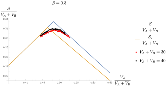
Refer to caption
Figure 33: Numerical evaluation of the von Neumann entropy of A𝐴A with αsubscript𝛼{{\mathcal{I}}}_{{\alpha}} as in (F.1) using the resolvent (F.3). We can see that the Page transition occurs at the point predicted by (2.49) and not at, for instance, the transition for the second Renyi entropy from (F.2). For simplicity, we have used a Gaussian density of states ρ(E)exp[E22NB]proportional-to𝜌𝐸superscript𝐸22subscript𝑁𝐵\rho(E)\propto\exp\left[-\frac{E^{2}}{2N_{B}}\right].

F.2 Microcanonical ensemble with different entropy densities in A𝐴A and B𝐵B

If we take the effective identity operator to be

α=p,q,EpA+EqA¯=E|pp|A|qq|B,subscript𝛼subscript𝑝𝑞subscriptsuperscript𝐸𝐴𝑝subscriptsuperscript𝐸¯𝐴𝑞𝐸tensor-productket𝑝subscriptbra𝑝𝐴ket𝑞subscriptbra𝑞𝐵{{\mathcal{I}}}_{{\alpha}}=\sum_{p,\,q,\,E^{A}_{p}+E^{\bar{A}}_{q}=E}\ket{p}\bra{p}_{A}\otimes\ket{q}\bra{q}_{B}, (F.4)

then the equilibrium approximation for 𝒵n(A)superscriptsubscript𝒵𝑛𝐴{\mathcal{Z}}_{n}^{(A)} in (2.38) gives

𝒵n(A)τ(dA)k(τη1)(dEB)k(τ)(NE)n,NE=dAdEBformulae-sequencesuperscriptsubscript𝒵𝑛𝐴subscript𝜏superscriptsuperscriptsubscript𝑑𝐴𝑘𝜏superscript𝜂1superscriptsubscriptsuperscript𝑑𝐵𝐸𝑘𝜏superscriptsubscript𝑁𝐸𝑛subscript𝑁𝐸subscriptsuperscriptsubscript𝑑𝐴subscriptsuperscript𝑑𝐵𝐸{\mathcal{Z}}_{n}^{(A)}\approx\sum_{\tau}{(d_{{{\mathcal{E}}}}^{A})^{k(\tau\eta^{-1})}(d^{B}_{E-{{\mathcal{E}}}})^{k(\tau)}\over(N_{E})^{n}},\quad N_{E}=\sum_{{{\mathcal{E}}}}d_{{{\mathcal{E}}}}^{A}\,d^{B}_{E-{{\mathcal{E}}}} (F.5)

Let us consider the resolvent

R(λ)𝑅𝜆\displaystyle R(\lambda) =1λn=0λn𝒵n(A)=1λn=0λn(dAdEB)nNEnτ(dA)k(τη1)(dEB)k(τ)(dAdEB)nabsent1𝜆superscriptsubscript𝑛0superscript𝜆𝑛superscriptsubscript𝒵𝑛𝐴subscript1𝜆superscriptsubscript𝑛0superscript𝜆𝑛superscriptsuperscriptsubscript𝑑𝐴subscriptsuperscript𝑑𝐵𝐸𝑛superscriptsubscript𝑁𝐸𝑛subscript𝜏superscriptsuperscriptsubscript𝑑𝐴𝑘𝜏superscript𝜂1superscriptsubscriptsuperscript𝑑𝐵𝐸𝑘𝜏superscriptsuperscriptsubscript𝑑𝐴subscriptsuperscript𝑑𝐵𝐸𝑛\displaystyle={1\over\lambda}\sum_{n=0}^{\infty}\lambda^{-n}{\mathcal{Z}}_{n}^{(A)}=\sum_{{{\mathcal{E}}}}{1\over\lambda}\sum_{n=0}^{\infty}\lambda^{-n}\frac{(d_{{{\mathcal{E}}}}^{A}d^{B}_{E-{{\mathcal{E}}}})^{n}}{N_{E}^{n}}\sum_{\tau}{(d_{{{\mathcal{E}}}}^{A})^{k(\tau\eta^{-1})}(d^{B}_{E-{{\mathcal{E}}}})^{k(\tau)}\over(d_{{{\mathcal{E}}}}^{A}d^{B}_{E-{{\mathcal{E}}}})^{n}} (F.6)
=NEdAdEBR(λ~;dA,dEB)=1pR(λ~;dA,dEB)absentsubscriptsubscript𝑁𝐸superscriptsubscript𝑑𝐴subscriptsuperscript𝑑𝐵𝐸subscript𝑅~𝜆superscriptsubscript𝑑𝐴subscriptsuperscript𝑑𝐵𝐸subscript1subscript𝑝subscript𝑅~𝜆superscriptsubscript𝑑𝐴subscriptsuperscript𝑑𝐵𝐸\displaystyle=\sum_{{{\mathcal{E}}}}{N_{E}\over d_{{{\mathcal{E}}}}^{A}d^{B}_{E-{{\mathcal{E}}}}}R_{\infty}(\tilde{\lambda};d_{{{\mathcal{E}}}}^{A},d^{B}_{E-{{\mathcal{E}}}})=\sum_{{\mathcal{E}}}{1\over p_{{\mathcal{E}}}}R_{\infty}(\tilde{\lambda};d_{{{\mathcal{E}}}}^{A},d^{B}_{E-{{\mathcal{E}}}})

where

R(λ;dA,dB)subscript𝑅𝜆subscript𝑑𝐴subscript𝑑𝐵\displaystyle R_{\infty}(\lambda;d_{A},d_{B}) =dAdB2λ+dAdB2dAdB2λ(λλ+)(λλ),absentsubscript𝑑𝐴subscript𝑑𝐵2𝜆subscript𝑑𝐴subscript𝑑𝐵2subscript𝑑𝐴subscript𝑑𝐵2𝜆𝜆subscript𝜆𝜆subscript𝜆\displaystyle=\frac{d_{A}-d_{B}}{2\lambda}+\frac{d_{A}d_{B}}{2}-\frac{d_{A}d_{B}}{2\lambda}\sqrt{\left(\lambda-\lambda_{+}\right)\left(\lambda-\lambda_{-}\right)}, (F.7)

is the resolvent for ρAsubscript𝜌𝐴\rho_{A} in the infinite temperature case, and

λ~=λNEdAdEB,p=dAdEBNE.formulae-sequence~𝜆𝜆subscript𝑁𝐸superscriptsubscript𝑑𝐴subscriptsuperscript𝑑𝐵𝐸subscript𝑝superscriptsubscript𝑑𝐴subscriptsuperscript𝑑𝐵𝐸subscript𝑁𝐸\tilde{\lambda}={\lambda N_{E}\over d_{{{\mathcal{E}}}}^{A}d^{B}_{E-{{\mathcal{E}}}}},\qquad p_{{\mathcal{E}}}={d_{{{\mathcal{E}}}}^{A}d^{B}_{E-{{\mathcal{E}}}}\over N_{E}}\ . (F.8)

(F.6) can be used to express the density of eigenvalues D(λ)𝐷𝜆D(\lambda) of ρAsubscript𝜌𝐴\rho_{A}, and its von Neumann and Renyi entropies, all in terms of their infinite temperature values,

D(λ)=1pD(λ~;dA,dEB)𝐷𝜆subscript1subscript𝑝subscript𝐷~𝜆superscriptsubscript𝑑𝐴subscriptsuperscript𝑑𝐵𝐸\displaystyle D(\lambda)=\sum_{{{\mathcal{E}}}}{1\over p_{{\mathcal{E}}}}D_{\infty}(\tilde{\lambda};d_{{{\mathcal{E}}}}^{A},d^{B}_{E-{{\mathcal{E}}}}) (F.9)
SA=Dλλlogλ=pSA()plogp,subscript𝑆𝐴𝐷𝜆𝜆𝜆subscriptsubscript𝑝superscriptsubscript𝑆𝐴subscriptsubscript𝑝subscript𝑝\displaystyle S_{A}=-\int D\lambda\,\lambda\log\lambda=\sum_{{\mathcal{E}}}p_{{\mathcal{E}}}S_{A}^{\infty}({{\mathcal{E}}})-\sum_{{\mathcal{E}}}p_{{\mathcal{E}}}\log p_{{{\mathcal{E}}}},\quad (F.10)
𝒵n,A=𝑑λD(λ)λn=(p)n𝒵n,A(dA;dEB).subscript𝒵𝑛𝐴differential-d𝜆𝐷𝜆superscript𝜆𝑛subscriptsuperscriptsubscript𝑝𝑛superscriptsubscript𝒵𝑛𝐴superscriptsubscript𝑑𝐴subscriptsuperscript𝑑𝐵𝐸\displaystyle{\mathcal{Z}}_{n,A}=\int d\lambda\,D(\lambda)\lambda^{n}=\sum_{{\mathcal{E}}}(p_{{\mathcal{E}}})^{n}\,{\mathcal{Z}}_{n,A}^{\infty}(d_{{{\mathcal{E}}}}^{A};d^{B}_{E-{{\mathcal{E}}}})\ . (F.11)

Let us first consider Sn(A)superscriptsubscript𝑆𝑛𝐴S_{n}^{(A)} for n1𝑛1n\neq 1. Since we know that

𝒵n,A(dA,dB)={dA1ndA<dBdB1ndB<dAsuperscriptsubscript𝒵𝑛𝐴subscript𝑑𝐴subscript𝑑𝐵casessuperscriptsubscript𝑑𝐴1𝑛subscript𝑑𝐴subscript𝑑𝐵superscriptsubscript𝑑𝐵1𝑛subscript𝑑𝐵subscript𝑑𝐴{\mathcal{Z}}_{n,A}^{\infty}(d_{A},d_{B})=\begin{cases}d_{A}^{1-n}&d_{A}<d_{B}\\ d_{B}^{1-n}&d_{B}<d_{A}\end{cases} (F.12)

we have

𝒵n,A=,dA<dEB(dEB)ndANEn+,dA>dEBdEB(dA)nNEnsubscript𝒵𝑛𝐴subscriptsubscriptsuperscript𝑑𝐴subscriptsuperscript𝑑𝐵𝐸superscriptsubscriptsuperscript𝑑𝐵𝐸𝑛subscriptsuperscript𝑑𝐴superscriptsubscript𝑁𝐸𝑛subscriptsubscriptsuperscript𝑑𝐴subscriptsuperscript𝑑𝐵𝐸subscriptsuperscript𝑑𝐵𝐸superscriptsubscriptsuperscript𝑑𝐴𝑛superscriptsubscript𝑁𝐸𝑛{\mathcal{Z}}_{n,A}=\sum_{{{\mathcal{E}}},\,d^{A}_{{{\mathcal{E}}}}<d^{B}_{E-{{\mathcal{E}}}}}\frac{(d^{B}_{E-{{\mathcal{E}}}})^{n}d^{A}_{{{\mathcal{E}}}}}{N_{E}^{n}}+\sum_{{{\mathcal{E}}},\,d^{A}_{{{\mathcal{E}}}}>d^{B}_{E-{{\mathcal{E}}}}}\frac{d^{B}_{E-{{\mathcal{E}}}}(d^{A}_{{{\mathcal{E}}}})^{n}}{N_{E}^{n}} (F.13)

Assuming that the saddle points for each of the above two integrals lie within their respective ranges, we then have

𝒵n,Ae(n1)Sn,A(eq)+e(n1)Sn,B(eq)Sn,A=min(Sn,A(eq),Sn,B(eq))formulae-sequencesubscript𝒵𝑛𝐴superscript𝑒𝑛1superscriptsubscript𝑆𝑛𝐴eqsuperscript𝑒𝑛1superscriptsubscript𝑆𝑛𝐵eqsubscript𝑆𝑛𝐴minsuperscriptsubscript𝑆𝑛𝐴eqsuperscriptsubscript𝑆𝑛𝐵eq{\mathcal{Z}}_{n,A}\approx e^{-(n-1)S_{n,A}^{\rm(eq)}}+e^{-(n-1)S_{n,B}^{\rm(eq)}}\quad\Rightarrow\quad S_{n,A}=\text{min}(S_{n,A}^{\rm(eq)},\,S_{n,B}^{\rm(eq)}) (F.14)

If we take the entropy densities in A𝐴A and B𝐵B to have distinct forms, for instance,

dEA=eVAsA(EVA),dEB=eVBsB(EVB),sA(ϵ)=gϵ1/2,sB(ϵ)=gϵ3/4,formulae-sequencesubscriptsuperscript𝑑𝐴𝐸superscript𝑒subscript𝑉𝐴subscript𝑠𝐴𝐸subscript𝑉𝐴formulae-sequencesubscriptsuperscript𝑑𝐵𝐸superscript𝑒subscript𝑉𝐵subscript𝑠𝐵𝐸subscript𝑉𝐵formulae-sequencesubscript𝑠𝐴italic-ϵ𝑔superscriptitalic-ϵ12subscript𝑠𝐵italic-ϵ𝑔superscriptitalic-ϵ34d^{A}_{E}=e^{V_{A}\,s_{A}(\frac{E}{V_{A}})},\quad d^{B}_{E}=e^{V_{B}\,s_{B}(\frac{E}{V_{B}})},\quad s_{A}(\epsilon)=g\,\epsilon^{1/2},\quad s_{B}(\epsilon)=g\,\epsilon^{3/4}\,, (F.15)

then as shown in Fig. 34, (F.14) implies that Snsubscript𝑆𝑛S_{n} for different n𝑛n transition from increasing to decreasing behaviour as a function of the volume fraction VAVsubscript𝑉𝐴𝑉\frac{V_{A}}{V} at different points.

Refer to caption
Figure 34: Renyi and von Neumann entropies as a function of volume fraction for the microcanonical ensemble with inhomogeneous entropy densities in A𝐴A and B𝐵B.

Let us now consider the von Neumann entropy in (F.10). We have

SA=dAdEBNEmin(logdA,logdEB)dAdEBNElog(dAdEBNE)subscript𝑆𝐴subscriptsubscriptsuperscript𝑑𝐴subscriptsuperscript𝑑𝐵𝐸subscript𝑁𝐸minsubscriptsuperscript𝑑𝐴subscriptsuperscript𝑑𝐵𝐸subscriptsubscriptsuperscript𝑑𝐴subscriptsuperscript𝑑𝐵𝐸subscript𝑁𝐸subscriptsuperscript𝑑𝐴subscriptsuperscript𝑑𝐵𝐸subscript𝑁𝐸\begin{gathered}S_{A}=\sum_{{{\mathcal{E}}}}\frac{d^{A}_{{{\mathcal{E}}}}d^{B}_{E-{{\mathcal{E}}}}}{N_{E}}\text{min}\left(\log d^{A}_{{{\mathcal{E}}}},\log d^{B}_{E-{{\mathcal{E}}}}\right)-\sum_{{{\mathcal{E}}}}\frac{d^{A}_{{{\mathcal{E}}}}d^{B}_{E-{{\mathcal{E}}}}}{N_{E}}\log\left(\frac{d^{A}_{{{\mathcal{E}}}}d^{B}_{E-{{\mathcal{E}}}}}{N_{E}}\right)\end{gathered} (F.16)

Let us evaluate each of the terms on the right-hand side in the saddle-point approximation. First note that

NE=dAdEB=VA𝑑ϵeVAsA(ϵ)+VBsB(EϵVAVB)2πBeSA(eq)+SB(eq)subscript𝑁𝐸subscriptsubscriptsuperscript𝑑𝐴subscriptsuperscript𝑑𝐵𝐸subscript𝑉𝐴differential-ditalic-ϵsuperscript𝑒subscript𝑉𝐴subscript𝑠𝐴italic-ϵsubscript𝑉𝐵subscript𝑠𝐵𝐸italic-ϵsubscript𝑉𝐴subscript𝑉𝐵2𝜋𝐵superscript𝑒subscriptsuperscript𝑆eq𝐴subscriptsuperscript𝑆eq𝐵N_{E}=\sum_{{{\mathcal{E}}}}d^{A}_{{{\mathcal{E}}}}d^{B}_{E-{{\mathcal{E}}}}=V_{A}\int d\epsilon~{}e^{V_{A}s_{A}(\epsilon)+V_{B}s_{B}\left(\frac{E-\epsilon V_{A}}{V_{B}}\right)}\approx\sqrt{\frac{2\pi}{B}}\,e^{S^{\rm(eq)}_{A}+S^{\rm(eq)}_{B}} (F.17)

where

B=1VAsA′′(ϵ¯A)1VBsB′′(ϵ¯B).𝐵1subscript𝑉𝐴subscriptsuperscript𝑠′′𝐴subscript¯italic-ϵ𝐴1subscript𝑉𝐵subscriptsuperscript𝑠′′𝐵subscript¯italic-ϵ𝐵B=-\frac{1}{V_{A}}s^{\prime\prime}_{A}(\bar{\epsilon}_{A})-\frac{1}{V_{B}}s^{\prime\prime}_{B}(\bar{\epsilon}_{B})\,. (F.18)

Note that the von Neumann entropies SA(eq)subscriptsuperscript𝑆eq𝐴S^{\rm(eq)}_{A} and SB(eq)subscriptsuperscript𝑆eq𝐵S^{\rm(eq)}_{B} appear here as they are respectively the values of VAsA(ϵ)subscript𝑉𝐴subscript𝑠𝐴italic-ϵV_{A}s_{A}(\epsilon) and VAsA(EVAϵVA¯)subscript𝑉𝐴subscript𝑠𝐴𝐸subscript𝑉𝐴italic-ϵsubscript𝑉¯𝐴V_{A}s_{A}(\frac{E-V_{A}\epsilon}{V_{\bar{A}}}) at the saddle-point value ϵ¯¯italic-ϵ\bar{\epsilon} of ϵitalic-ϵ\epsilon, which is the solution to

sA(ϵ¯)=sB(EVAϵ¯VB).subscriptsuperscript𝑠𝐴¯italic-ϵsubscriptsuperscript𝑠𝐵𝐸subscript𝑉𝐴¯italic-ϵsubscript𝑉𝐵s^{\prime}_{A}(\bar{\epsilon})=s^{\prime}_{B}\left(\frac{E-V_{A}\bar{\epsilon}}{V_{B}}\right)\,. (F.19)

We can use the saddle-point approximation for the second term in (F.16) to see that it gives a contribution at O(logV)𝑂𝑉O(\log V). The saddle-point approximation for the first term is

SAVA𝑑ϵe12BVA2(ϵϵ¯)22π/Bmin(SA(eq)+VAβ(ϵϵ¯)+,SB(eq)VAβ(ϵϵ¯)+)subscript𝑆𝐴subscript𝑉𝐴differential-ditalic-ϵsuperscript𝑒12𝐵superscriptsubscript𝑉𝐴2superscriptitalic-ϵ¯italic-ϵ22𝜋𝐵minsubscriptsuperscript𝑆eq𝐴subscript𝑉𝐴𝛽italic-ϵ¯italic-ϵsubscriptsuperscript𝑆eq𝐵subscript𝑉𝐴𝛽italic-ϵ¯italic-ϵ\begin{gathered}S_{A}\approx V_{A}\int d\epsilon\frac{e^{-\frac{1}{2}B\,V_{A}^{2}\,(\epsilon-\bar{\epsilon})^{2}}}{\sqrt{2\pi/B}}\text{min}(S^{\rm(eq)}_{A}+V_{A}\beta(\epsilon-\bar{\epsilon})+...\,,\,S^{\rm(eq)}_{B}-V_{A}\beta(\epsilon-\bar{\epsilon})+...\,)\end{gathered} (F.20)

Assume without loss of generality that SA(eq)<SB(eq)subscriptsuperscript𝑆eq𝐴subscriptsuperscript𝑆eq𝐵S^{\rm(eq)}_{A}<S^{\rm(eq)}_{B}. We can write

SASA(eq)B2πVA2VAβ(ϵϵ¯)SB(eq)SA(eq)𝑑ϵe12BVA2(ϵϵ¯)2+B2πVA2VAβ(ϵϵ¯)SB(eq)SA(eq)𝑑ϵe12BVA2(ϵϵ¯)2VAβ(ϵϵ¯)+B2πVA2VAβ(ϵϵ¯)>SB(eq)SA(eq)𝑑ϵe12BVA2(ϵϵ¯)2(SB(eq)VAβ(ϵϵ¯))subscript𝑆𝐴subscriptsuperscript𝑆eq𝐴𝐵2𝜋subscript𝑉𝐴subscript2subscript𝑉𝐴𝛽italic-ϵ¯italic-ϵsuperscriptsubscript𝑆𝐵eqsuperscriptsubscript𝑆𝐴eqdifferential-ditalic-ϵsuperscript𝑒12𝐵superscriptsubscript𝑉𝐴2superscriptitalic-ϵ¯italic-ϵ2𝐵2𝜋subscript𝑉𝐴subscript2subscript𝑉𝐴𝛽italic-ϵ¯italic-ϵsuperscriptsubscript𝑆𝐵eqsuperscriptsubscript𝑆𝐴eqdifferential-ditalic-ϵsuperscript𝑒12𝐵superscriptsubscript𝑉𝐴2superscriptitalic-ϵ¯italic-ϵ2subscript𝑉𝐴𝛽italic-ϵ¯italic-ϵ𝐵2𝜋subscript𝑉𝐴subscript2subscript𝑉𝐴𝛽italic-ϵ¯italic-ϵsuperscriptsubscript𝑆𝐵eqsuperscriptsubscript𝑆𝐴eqdifferential-ditalic-ϵsuperscript𝑒12𝐵superscriptsubscript𝑉𝐴2superscriptitalic-ϵ¯italic-ϵ2subscriptsuperscript𝑆eq𝐵subscript𝑉𝐴𝛽italic-ϵ¯italic-ϵ\begin{gathered}S_{A}\approx S^{\rm(eq)}_{A}\,\sqrt{\frac{B}{2\pi}}V_{A}\int_{2V_{A}\beta(\epsilon-\bar{\epsilon})\leq S_{B}^{\rm(eq)}-S_{A}^{\rm(eq)}}d\epsilon\,e^{-\frac{1}{2}B\,V_{A}^{2}\,(\epsilon-\bar{\epsilon})^{2}}\,\\ +\sqrt{\frac{B}{2\pi}}V_{A}\int_{2V_{A}\beta(\epsilon-\bar{\epsilon})\leq S_{B}^{\rm(eq)}-S_{A}^{\rm(eq)}}d\epsilon\,e^{-\frac{1}{2}B\,V_{A}^{2}\,(\epsilon-\bar{\epsilon})^{2}}\,V_{A}\beta(\epsilon-\bar{\epsilon})\\ +\sqrt{\frac{B}{2\pi}}V_{A}\int_{2V_{A}\beta(\epsilon-\bar{\epsilon})>S_{B}^{\rm(eq)}-S_{A}^{\rm(eq)}}\,d\epsilon\,e^{-\frac{1}{2}B\,V_{A}^{2}\,(\epsilon-\bar{\epsilon})^{2}}\,(S^{\rm(eq)}_{B}-V_{A}\beta(\epsilon-\bar{\epsilon}))\end{gathered} (F.21)

Let us consider the above expression in different regimes of the difference SB(eq)SA(eq)subscriptsuperscript𝑆eq𝐵subscriptsuperscript𝑆eq𝐴S^{\rm(eq)}_{B}-S^{\rm(eq)}_{A}.

  1. 1.

    If SB(eq)SA(eq)1Bmuch-greater-thansubscriptsuperscript𝑆eq𝐵superscriptsubscript𝑆𝐴eq1𝐵S^{\rm(eq)}_{B}-S_{A}^{\rm(eq)}\gg\frac{1}{\sqrt{B}}, then the first term in (F.21) is approximately SAsubscript𝑆𝐴S_{A}, while the remaining terms are approximately zero.

  2. 2.

    If SA(eq)=SB(eq)subscriptsuperscript𝑆eq𝐴subscriptsuperscript𝑆eq𝐵S^{\rm(eq)}_{A}=S^{\rm(eq)}_{B}, then (F.21) becomes

    SAsubscript𝑆𝐴\displaystyle S_{A} =SA(eq)B2πVA𝑑ϵe12BVA2(ϵϵ¯)2B2πVA𝑑ϵe12BVA2(ϵϵ¯)2VAβ|ϵϵ¯|absentsubscriptsuperscript𝑆eq𝐴𝐵2𝜋subscript𝑉𝐴superscriptsubscriptdifferential-ditalic-ϵsuperscript𝑒12𝐵superscriptsubscript𝑉𝐴2superscriptitalic-ϵ¯italic-ϵ2𝐵2𝜋subscript𝑉𝐴superscriptsubscriptdifferential-ditalic-ϵsuperscript𝑒12𝐵superscriptsubscript𝑉𝐴2superscriptitalic-ϵ¯italic-ϵ2subscript𝑉𝐴𝛽italic-ϵ¯italic-ϵ\displaystyle=S^{\rm(eq)}_{A}\,\sqrt{\frac{B}{2\pi}}V_{A}\int_{-\infty}^{\infty}d\epsilon\,e^{-\frac{1}{2}B\,V_{A}^{2}\,(\epsilon-\bar{\epsilon})^{2}}-\sqrt{\frac{B}{2\pi}}V_{A}\int_{-\infty}^{\infty}d\epsilon\,e^{-\frac{1}{2}B\,V_{A}^{2}\,(\epsilon-\bar{\epsilon})^{2}}\,V_{A}\beta|\epsilon-\bar{\epsilon}|
    =SA(eq)2β2πBabsentsubscriptsuperscript𝑆eq𝐴2superscript𝛽2𝜋𝐵\displaystyle=S^{\rm(eq)}_{A}-\sqrt{\frac{2\beta^{2}}{\pi B}} (F.22)
  3. 3.

    If SB(eq)SA(eq)1Bsimilar-tosuperscriptsubscript𝑆𝐵eqsuperscriptsubscript𝑆𝐴eq1𝐵S_{B}^{\rm(eq)}-S_{A}^{\rm(eq)}\sim\frac{1}{\sqrt{B}}, then the three terms in (F.21) should be evaluated more carefully, and we get corrections to the value of SA(eq)subscriptsuperscript𝑆eq𝐴S^{\rm(eq)}_{A} of order V𝑉\sqrt{V}. This gives a smoothed out transition between the increasing and decreasing parts of the Page curve as a function of VAsubscript𝑉𝐴V_{A}. However, since SA(eq)superscriptsubscript𝑆𝐴eqS_{A}^{\rm(eq)} and SB(eq)superscriptsubscript𝑆𝐵eqS_{B}^{\rm(eq)} scale roughly linearly with VAsubscript𝑉𝐴V_{A} and VBsubscript𝑉𝐵V_{B}, the smoothing out of the transition is over a range of values of VAsubscript𝑉𝐴V_{A} of order V𝑉\sqrt{V}. So as a function of the parameter c:=VAVassign𝑐subscript𝑉𝐴𝑉c:=\frac{V_{A}}{V}, the transition between the increasing and decreasing parts of the Page curve is still sharp in the thermodynamic limit.

The observations about enhanced corrections of order V𝑉\sqrt{V} close to the Page transition in points 2 and 3 were made earlier in [59] and [60]. Similar effects were observed in the canonical ensemble in the model of [4]. Since we are interested in the sharp transition as a function of c𝑐c in this discussion, we can ignore the effects of such corrections, and we then find that at leading order (F.20) implies

SA=min(SA(eq),SB(eq)),subscript𝑆𝐴minsuperscriptsubscript𝑆𝐴eqsuperscriptsubscript𝑆𝐵eqS_{A}=\text{min}(S_{A}^{\rm(eq)},S_{B}^{\rm(eq)}), (F.23)

confirming (2.49) for this example. As shown in Fig. 34, when we take the inhomogeneous entropy densities in (F.15), the Page transition of the von Neumann entropy coming from (F.23) takes place at a distinct value of VAVsubscript𝑉𝐴𝑉\frac{V_{A}}{V} from the transitions of each of Renyi entropies from (F.14).

Appendix G Evolution of Petz map fidelity at finite temperature

G.1 Canonical ensemble

To evaluate the fidelity of the Petz map reconstruction F(ρ,[𝒫σ,𝒩𝒩](ρ))𝐹𝜌delimited-[]subscript𝒫𝜎𝒩𝒩𝜌F(\rho,[\mathcal{P}_{\sigma,\mathcal{N}}\circ\mathcal{N}](\rho)) systematically at finite temperature for the canonical ensemble, we use a method similar to Section 3 of [4]. We take the reference state σDsubscript𝜎𝐷\sigma_{D} to be maximally mixed and ρDsubscript𝜌𝐷\rho_{D} to be pure. For simplicity, we take R𝑅R to be at infinite temperature, so that the effective identity operator is

α=eβHB𝟏R.subscript𝛼tensor-productsuperscript𝑒𝛽subscript𝐻superscript𝐵subscript1𝑅{{\mathcal{I}}}_{{\alpha}}=e^{-\beta H_{B^{\prime}}}\otimes\mathbf{1}_{R}\,. (G.1)

It is useful to define

Fn1,n2Fn1,n2c+Fn1,n2dsubscript𝐹subscript𝑛1subscript𝑛2subscriptsuperscript𝐹𝑐subscript𝑛1subscript𝑛2subscriptsuperscript𝐹𝑑subscript𝑛1subscript𝑛2F_{n_{1},n_{2}}\equiv F^{c}_{n_{1},n_{2}}+F^{d}_{n_{1},n_{2}} (G.2)

for two non-negative integers n1,n2subscript𝑛1subscript𝑛2n_{1},n_{2}, where

Fn1,n2c1Z1n1+n2+21dDn1+n2+2τPcηReB|α,τdDk(τ)subscriptsuperscript𝐹𝑐subscript𝑛1subscript𝑛21superscriptsubscript𝑍1subscript𝑛1subscript𝑛221superscriptsubscript𝑑𝐷subscript𝑛1subscript𝑛22subscript𝜏subscript𝑃𝑐inner-producttensor-productsubscript𝜂𝑅subscript𝑒superscript𝐵subscript𝛼𝜏superscriptsubscript𝑑𝐷𝑘𝜏\displaystyle F^{c}_{n_{1},n_{2}}\equiv\frac{1}{Z_{1}^{n_{1}+n_{2}+2}}\frac{1}{d_{D}^{n_{1}+n_{2}+2}}\sum_{\tau\in P_{c}}\braket{\eta_{R}\otimes e_{B^{\prime}}}{{{\mathcal{I}}}_{{\alpha}},\tau}d_{D}^{k(\tau)} (G.3)
Fn1,n2d1Z1n1+n2+21dDn1+n2+3τPdηReB|α,τdDk(τ)subscriptsuperscript𝐹𝑑subscript𝑛1subscript𝑛21superscriptsubscript𝑍1subscript𝑛1subscript𝑛221superscriptsubscript𝑑𝐷subscript𝑛1subscript𝑛23subscript𝜏subscript𝑃𝑑inner-producttensor-productsubscript𝜂𝑅subscript𝑒superscript𝐵subscript𝛼𝜏superscriptsubscript𝑑𝐷𝑘𝜏\displaystyle F^{d}_{n_{1},n_{2}}\equiv\frac{1}{Z_{1}^{n_{1}+n_{2}+2}}\frac{1}{d_{D}^{n_{1}+n_{2}+3}}\sum_{\tau\in P_{d}}\braket{\eta_{R}\otimes e_{B^{\prime}}}{{{\mathcal{I}}}_{{\alpha}},\tau}d_{D}^{k(\tau)} (G.4)

where Pcsubscript𝑃𝑐P_{c} refers to the set of permutations in Sn1+n2+2subscript𝑆subscript𝑛1subscript𝑛22S_{n_{1}+n_{2}+2} such that the first and n1+2subscript𝑛12n_{1}+2-th element are in the same cycle, and Pdsubscript𝑃𝑑P_{d} refers to the rest. The equilibrium approximation for the fidelity is then given by 212121Note that here we use the alternative analytic continuation from (2.69).

F(ρ,[𝒫σ,𝒩𝒩](ρ))=Fc+Fd,Fc,d=limn112,n212Fn1,n2c,dformulae-sequence𝐹𝜌delimited-[]subscript𝒫𝜎𝒩𝒩𝜌superscript𝐹𝑐superscript𝐹𝑑superscript𝐹𝑐𝑑subscriptformulae-sequencesubscript𝑛112subscript𝑛212subscriptsuperscript𝐹𝑐𝑑subscript𝑛1subscript𝑛2F(\rho,[\mathcal{P}_{\sigma,\mathcal{N}}\circ\mathcal{N}](\rho))=F^{c}+F^{d},\quad F^{c,d}=\lim_{n_{1}\rightarrow-{{\frac{1}{2}}},\,n_{2}\rightarrow-{{\frac{1}{2}}}}F^{c,d}_{n_{1},n_{2}} (G.5)

Note that

Fn1,n2c+dDFn1,n2dsubscriptsuperscript𝐹𝑐subscript𝑛1subscript𝑛2subscript𝑑𝐷subscriptsuperscript𝐹𝑑subscript𝑛1subscript𝑛2\displaystyle F^{c}_{n_{1},n_{2}}+d_{D}F^{d}_{n_{1},n_{2}} =1(Z1dD)n1+n2+2τSn1+n2+2ηReBeD|(α)BR𝟏D,τabsent1superscriptsubscript𝑍1subscript𝑑𝐷subscript𝑛1subscript𝑛22subscript𝜏subscript𝑆subscript𝑛1subscript𝑛22inner-producttensor-productsubscript𝜂𝑅subscript𝑒superscript𝐵subscript𝑒superscript𝐷tensor-productsubscriptsubscript𝛼superscript𝐵𝑅subscript1superscript𝐷𝜏\displaystyle=\frac{1}{(Z_{1}d_{D})^{n_{1}+n_{2}+2}}\sum_{\tau\in S_{n_{1}+n_{2}+2}}\braket{\eta_{R}\otimes e_{B^{\prime}}\otimes e_{D^{\prime}}}{({{\mathcal{I}}}_{{\alpha}})_{B^{\prime}R}\otimes\mathbf{1}_{D^{\prime}},\tau} (G.6)
=𝒵n1+n2+2,Rabsentsubscript𝒵subscript𝑛1subscript𝑛22𝑅\displaystyle={\mathcal{Z}}_{n_{1}+n_{2}+2,R} (G.7)

where we get the last expression by identifying the second-to-last expression to be the equilibrium approximation for 𝒵n1+n2+2,Rsubscript𝒵subscript𝑛1subscript𝑛22𝑅{\mathcal{Z}}_{n_{1}+n_{2}+2,R} for an equilibrated pure state |ΨketΨ\ket{\Psi} in a Hilbert space BRDtensor-productsubscriptsuperscript𝐵𝑅subscriptsuperscript𝐷{{\mathcal{H}}}_{B^{\prime}R}\otimes{{\mathcal{H}}}_{D^{\prime}}, with the effective identity operator (α)BR𝟏Dtensor-productsubscriptsubscript𝛼superscript𝐵𝑅subscript1superscript𝐷({{\mathcal{I}}}_{{\alpha}})_{B^{\prime}R}\otimes\mathbf{1}_{D^{\prime}}, where Dsuperscript𝐷D^{\prime} is an auxiliary system with Hilbert space dimension dDsubscript𝑑𝐷d_{D}. This implies that

Fc+dDFd=𝒵1,R=1,superscript𝐹𝑐subscript𝑑𝐷superscript𝐹𝑑subscript𝒵1𝑅1F^{c}+d_{D}F^{d}={\mathcal{Z}}_{1,R}=1\,, (G.8)

so that it is sufficient to calculate Fcsuperscript𝐹𝑐F^{c} and express the fidelity as

F(ρ,[𝒫σ,𝒩𝒩](ρ))=(11dD)Fc+1dD.𝐹𝜌delimited-[]subscript𝒫𝜎𝒩𝒩𝜌11subscript𝑑𝐷superscript𝐹𝑐1subscript𝑑𝐷F(\rho,[\mathcal{P}_{\sigma,\mathcal{N}}\circ\mathcal{N}](\rho))=\left(1-\frac{1}{d_{D}}\right)F^{c}+\frac{1}{d_{D}}\,. (G.9)

In order to systematically obtain Fcsuperscript𝐹𝑐F^{c} using Fn1,n2csubscriptsuperscript𝐹𝑐subscript𝑛1subscript𝑛2F^{c}_{n_{1},n_{2}}, we can define the generating functional

Fc(λ1,λ2)=n1,n2=0Fn1,n2cλ1n1λ2n2.superscript𝐹𝑐subscript𝜆1subscript𝜆2superscriptsubscriptsubscript𝑛1subscript𝑛20subscriptsuperscript𝐹𝑐subscript𝑛1subscript𝑛2superscriptsubscript𝜆1subscript𝑛1superscriptsubscript𝜆2subscript𝑛2F^{c}(\lambda_{1},\lambda_{2})=\sum_{n_{1},n_{2}=0}^{\infty}\frac{F^{c}_{n_{1},n_{2}}}{\lambda_{1}^{n_{1}}\lambda_{2}^{n_{2}}}\,. (G.10)

Then for non-negative integers n1,n2subscript𝑛1subscript𝑛2n_{1},n_{2},

Fn1,n2c=dλ12πidλ22πiλ1n11λ2n21Fc(λ1,λ2)subscriptsuperscript𝐹𝑐subscript𝑛1subscript𝑛2subscriptcontour-integral𝑑subscript𝜆12𝜋𝑖𝑑subscript𝜆22𝜋𝑖superscriptsubscript𝜆1subscript𝑛11superscriptsubscript𝜆2subscript𝑛21superscript𝐹𝑐subscript𝜆1subscript𝜆2F^{c}_{n_{1},n_{2}}=\oint_{\infty}\frac{d\lambda_{1}}{2\pi i}\frac{d\lambda_{2}}{2\pi i}\,\lambda_{1}^{n_{1}-1}\lambda_{2}^{n_{2}-1}\,F^{c}(\lambda_{1},\lambda_{2}) (G.11)

where the contour is taken to be around the point at infinity. Now in all permutations τ𝜏\tau contributing to (G.10), the first and (n1+2)thsuperscriptsubscript𝑛12𝑡(n_{1}+2)^{th} element are in a common cycle. Suppose this cycle also includes m1subscript𝑚1m_{1} elements out of the n1subscript𝑛1n_{1} elements between the first and (n1+2)thsuperscriptsubscript𝑛12𝑡(n_{1}+2)^{th} element, and m2subscript𝑚2m_{2} elements after the (n1+2)thsuperscriptsubscript𝑛12𝑡(n_{1}+2)^{th} element. We can then consider the total contribution from a fixed m1subscript𝑚1m_{1}, m2subscript𝑚2m_{2} to all n1,n2subscript𝑛1subscript𝑛2n_{1},n_{2}, as shown in Figure 35. Note that in the process we have introduced factors of R(λ)𝑅𝜆R(\lambda), the resolvent for ρRTrBD[|ΨΨ|]subscript𝜌𝑅subscriptTrsuperscript𝐵superscript𝐷delimited-[]ketΨbraΨ\rho_{R}\equiv\text{Tr}_{B^{\prime}D^{\prime}}[\ket{\Psi}\bra{\Psi}], with |ΨketΨ\ket{\Psi} as defined above (G.8).

Refer to caption
Figure 35: Contribution from a fixed m1=2subscript𝑚12m_{1}=2 and m2=1subscript𝑚21m_{2}=1 to all n1subscript𝑛1n_{1} and n2subscript𝑛2n_{2} in the expression for Fc(λ1,λ2)superscript𝐹𝑐subscript𝜆1subscript𝜆2F^{c}(\lambda_{1},\lambda_{2}) in (G.10). The solid loop gives a factor of dDZm1+m2+2,B(dDdRZ1,B)m1+m2+2subscript𝑑𝐷subscript𝑍subscript𝑚1subscript𝑚22superscript𝐵superscriptsubscript𝑑𝐷subscript𝑑𝑅subscript𝑍1superscript𝐵subscript𝑚1subscript𝑚22\frac{d_{D}Z_{m_{1}+m_{2}+2,B^{\prime}}}{(d_{D}d_{R}Z_{1,B^{\prime}})^{m_{1}+m_{2}+2}}, and we get m1subscript𝑚1m_{1}, m1+1subscript𝑚11m_{1}+1, m2subscript𝑚2m_{2} and m2+1subscript𝑚21m_{2}+1 factors respectively of 1λ11subscript𝜆1\frac{1}{\lambda_{1}}, λ1R(λ1)subscript𝜆1𝑅subscript𝜆1\lambda_{1}R(\lambda_{1}), 1λ21subscript𝜆2\frac{1}{\lambda_{2}} and λ2R(λ2)subscript𝜆2𝑅subscript𝜆2\lambda_{2}R(\lambda_{2}), leading to (G.12).

We then find

Fc(λ1,λ2)=m1,m2=0dDZm1+m2+2,B(Z1,BdRdD)m1+m2+2R(λ1)m1+1R(λ2)m2+1λ1λ2.superscript𝐹𝑐subscript𝜆1subscript𝜆2superscriptsubscriptsubscript𝑚1subscript𝑚20subscript𝑑𝐷subscript𝑍subscript𝑚1subscript𝑚22superscript𝐵superscriptsubscript𝑍1superscript𝐵subscript𝑑𝑅subscript𝑑𝐷subscript𝑚1subscript𝑚22𝑅superscriptsubscript𝜆1subscript𝑚11𝑅superscriptsubscript𝜆2subscript𝑚21subscript𝜆1subscript𝜆2F^{c}(\lambda_{1},\lambda_{2})=\sum_{m_{1},m_{2}=0}^{\infty}\frac{d_{D}Z_{m_{1}+m_{2}+2,B^{\prime}}}{(Z_{1,B^{\prime}}\,d_{R}\,d_{D})^{m_{1}+m_{2}+2}}\,R(\lambda_{1})^{m_{1}+1}R(\lambda_{2})^{m_{2}+1}\,\lambda_{1}\lambda_{2}\,. (G.12)

and using (G.11),

Fn1,n2c=dD0𝑑Eρ(E)(dλ2πiλn1R(λ)eβEZ1,BdD1dReβER(λ)Z1,BdD)×(dλ2πiλn2R(λ)eβEZ1,BdD1dReβER(λ)Z1,BdD)subscriptsuperscript𝐹𝑐subscript𝑛1subscript𝑛2subscript𝑑𝐷superscriptsubscript0differential-d𝐸𝜌𝐸subscriptcontour-integral𝑑𝜆2𝜋𝑖superscript𝜆subscript𝑛1𝑅𝜆superscript𝑒𝛽𝐸subscript𝑍1superscript𝐵subscript𝑑𝐷1subscript𝑑𝑅superscript𝑒𝛽𝐸𝑅𝜆subscript𝑍1superscript𝐵subscript𝑑𝐷subscriptcontour-integral𝑑𝜆2𝜋𝑖superscript𝜆subscript𝑛2𝑅𝜆superscript𝑒𝛽𝐸subscript𝑍1superscript𝐵subscript𝑑𝐷1subscript𝑑𝑅superscript𝑒𝛽𝐸𝑅𝜆subscript𝑍1superscript𝐵subscript𝑑𝐷\begin{gathered}F^{c}_{n_{1},n_{2}}=d_{D}\int_{0}^{\infty}dE\,\rho(E)\,\left(\oint_{\infty}\frac{d\lambda}{2\pi i}\lambda^{n_{1}}R(\lambda)\frac{e^{-\beta E}}{Z_{1,B^{\prime}}d_{D}}\frac{1}{d_{R}-\frac{e^{-\beta E}R(\lambda)}{Z_{1,B^{\prime}}d_{D}}}\right)\\ \times\,\left(\oint_{\infty}\frac{d\lambda}{2\pi i}\lambda^{n_{2}}R(\lambda)\frac{e^{-\beta E}}{Z_{1,B^{\prime}}d_{D}}\frac{1}{d_{R}-\frac{e^{-\beta E}R(\lambda)}{Z_{1,B^{\prime}}d_{D}}}\right)\end{gathered} (G.13)

Note that λ12superscript𝜆12\lambda^{-{{\frac{1}{2}}}} has a branch point at infinity, so the above expression cannot be analytically continued as written. However, we can first deform the contour for integer n1,n2subscript𝑛1subscript𝑛2n_{1},n_{2} to surround the branch cut on the real axis coming from R(λ)𝑅𝜆R(\lambda), and then analytically continue to n1=n2=12subscript𝑛1subscript𝑛212n_{1}=n_{2}=-{{\frac{1}{2}}}, to get

Fc=dD0𝑑Eρ(E)(𝒞dλ2πiλ12R(λ)eβEZ1,BdD1dReβER(λ)Z1,BdD)2superscript𝐹𝑐subscript𝑑𝐷superscriptsubscript0differential-d𝐸𝜌𝐸superscriptsubscriptcontour-integral𝒞𝑑𝜆2𝜋𝑖superscript𝜆12𝑅𝜆superscript𝑒𝛽𝐸subscript𝑍1superscript𝐵subscript𝑑𝐷1subscript𝑑𝑅superscript𝑒𝛽𝐸𝑅𝜆subscript𝑍1superscript𝐵subscript𝑑𝐷2\begin{gathered}F^{c}=d_{D}\int_{0}^{\infty}dE\,\rho(E)\,\left(\oint_{{{\mathcal{C}}}}\frac{d\lambda}{2\pi i}\lambda^{-{{\frac{1}{2}}}}R(\lambda)\frac{e^{-\beta E}}{Z_{1,B^{\prime}}d_{D}}\frac{1}{d_{R}-\frac{e^{-\beta E}R(\lambda)}{Z_{1,B^{\prime}}d_{D}}}\right)^{2}\end{gathered} (G.14)

where 𝒞𝒞{{\mathcal{C}}} is the contour that surrounds the branch cut on the real axis. In order to further simplify this expression, we use the following approximation for the resolvent:

R(λ)dRλλ0𝑅𝜆subscript𝑑𝑅𝜆subscript𝜆0R(\lambda)\approx\frac{d_{R}}{\lambda-\lambda_{0}}\, (G.15)

where λ0subscript𝜆0\lambda_{0} is the smallest eigenvalue of ρRsubscript𝜌𝑅\rho_{R}, which turns out to be

λ0=1dRg,g=1Z1,BE0𝑑Eρ(E)eβEformulae-sequencesubscript𝜆01subscript𝑑𝑅𝑔𝑔1subscript𝑍1superscript𝐵superscriptsubscriptsubscript𝐸0differential-d𝐸𝜌𝐸superscript𝑒𝛽𝐸\lambda_{0}=\frac{1}{d_{R}}g,\quad g=\frac{1}{Z_{1,B^{\prime}}}\int_{E_{0}}^{\infty}dE\,\rho(E)\,e^{-\beta E} (G.16)

with E0subscript𝐸0E_{0} defined through

0E0𝑑Eρ(E)=dRdD.superscriptsubscript0subscript𝐸0differential-d𝐸𝜌𝐸subscript𝑑𝑅subscript𝑑𝐷\int_{0}^{E_{0}}dE\,\rho(E)=\frac{d_{R}}{d_{D}}\,. (G.17)

In deriving (G.15)-(G.17), we use similar methods to [4], which we review for this context at the end of this subsection. Putting (G.15) into (G.14), we find

Fc1Z1,B0𝑑Eρ(E)e2βEdDZ1,Bλ0+eβE.superscript𝐹𝑐1subscript𝑍1superscript𝐵superscriptsubscript0differential-d𝐸𝜌𝐸superscript𝑒2𝛽𝐸subscript𝑑𝐷subscript𝑍1superscript𝐵subscript𝜆0superscript𝑒𝛽𝐸F^{c}\approx\frac{1}{Z_{1,B^{\prime}}}\int_{0}^{\infty}dE\,\rho(E)\,\frac{e^{-2\beta E}}{d_{D}Z_{1,B^{\prime}}\lambda_{0}+{e^{-\beta E}}}\,. (G.18)

Now to further analyse (G.18), let us take the density of states to be as in AdS3𝐴𝑑subscript𝑆3AdS_{3}, ρ(E)=ecVE/V𝜌𝐸superscript𝑒𝑐𝑉𝐸𝑉\rho(E)=e^{cV\sqrt{E/V}}, where V𝑉V is the volume of Bsuperscript𝐵B^{\prime}. Then Z1,Bsubscript𝑍1superscript𝐵Z_{1,B^{\prime}} can be evaluated using the saddle point approximation and has the behavior

Z1,B=cV12eβEc+cVϵc=cV12ec2V4β,Ec=Vϵc,ϵc=c2β,S=Vc22βformulae-sequencesubscript𝑍1superscript𝐵superscript𝑐superscript𝑉12superscript𝑒𝛽subscript𝐸𝑐𝑐𝑉subscriptitalic-ϵ𝑐superscript𝑐superscript𝑉12superscript𝑒superscript𝑐2𝑉4𝛽formulae-sequencesubscript𝐸𝑐𝑉subscriptitalic-ϵ𝑐formulae-sequencesubscriptitalic-ϵ𝑐𝑐2𝛽𝑆𝑉superscript𝑐22𝛽Z_{1,B^{\prime}}=c^{\prime}V^{{\frac{1}{2}}}e^{-{\beta}E_{c}+cV\sqrt{\epsilon_{c}}}=c^{\prime}V^{{\frac{1}{2}}}e^{{c^{2}V\over 4{\beta}}},\quad E_{c}=V\epsilon_{c},\quad\sqrt{\epsilon_{c}}={c\over 2{\beta}},\quad S=V{c^{2}\over 2{\beta}} (G.19)

where S𝑆S is the thermal entropy and csuperscript𝑐c^{\prime} is some O(1)𝑂1O(1) constant. The second equilibrium Renyi entropy can also be evaluated from the saddle point

eS2,B=Z1,B(2β)Z1,B2(β)V12e3c2V8β,S2,B=3c2V8β.formulae-sequencesuperscript𝑒subscript𝑆2superscript𝐵subscript𝑍1superscript𝐵2𝛽superscriptsubscript𝑍1superscript𝐵2𝛽similar-tosuperscript𝑉12superscript𝑒3superscript𝑐2𝑉8𝛽subscript𝑆2superscript𝐵3superscript𝑐2𝑉8𝛽e^{-S_{2,B^{\prime}}}={Z_{1,B^{\prime}}(2{\beta})\over Z_{1,B^{\prime}}^{2}({\beta})}\sim V^{-{{\frac{1}{2}}}}e^{-{3c^{2}V\over 8{\beta}}},\quad S_{2,B^{\prime}}={3c^{2}V\over 8{\beta}}\ . (G.20)

Now if we define

xlogdRV,ylogdDV,formulae-sequence𝑥subscript𝑑𝑅𝑉𝑦subscript𝑑𝐷𝑉x\equiv{\log d_{R}\over V},\quad y\equiv{\log d_{D}\over V}, (G.21)

then the various relevant time scales are given by:

tb:x=3c28β,tp:x=c22β,tp2:x=c22β+y.t_{b}:\quad x={3c^{2}\over 8{\beta}},\quad t_{p}:\quad x={c^{2}\over 2{\beta}},\quad t_{p_{2}}:\quad x={c^{2}\over 2{\beta}}+y\ . (G.22)

We will always take xO(1)similar-to𝑥𝑂1x\sim O(1) while take V𝑉V\to\infty, but y𝑦y can be O(V1)𝑂superscript𝑉1O(V^{-1}) or O(1)𝑂1O(1) depending on whether the diary is “small” or “large.”

Now let us examine the behavior of g𝑔g defined in (G.16). Note that for ϵ0=E0/Vsubscriptitalic-ϵ0subscript𝐸0𝑉\epsilon_{0}=E_{0}/V,

V0ϵ0𝑑ϵecVϵ=2cVϵ0ecVϵ0=dRdD𝑉superscriptsubscript0subscriptitalic-ϵ0differential-ditalic-ϵsuperscript𝑒𝑐𝑉italic-ϵ2𝑐𝑉subscriptitalic-ϵ0superscript𝑒𝑐𝑉subscriptitalic-ϵ0subscript𝑑𝑅subscript𝑑𝐷\displaystyle V\int_{0}^{\epsilon_{0}}d\epsilon\,e^{cV\sqrt{\epsilon}}={2\over cV}\sqrt{\epsilon_{0}}e^{cV\sqrt{\epsilon_{0}}}={d_{R}\over d_{D}} (G.23)
ϵ0xyc+O(V1logV),.subscriptitalic-ϵ0𝑥𝑦𝑐𝑂superscript𝑉1𝑉\displaystyle\quad\Rightarrow\quad\sqrt{\epsilon_{0}}\approx{x-y\over c}+O(V^{-1}\log V),\quad\ . (G.24)

so that g𝑔g has the form

g=12[1+erf(Vβ(ϵcϵ0))]+βπc2VeVβ(ϵcϵ0)2𝑔12delimited-[]1erf𝑉𝛽subscriptitalic-ϵ𝑐subscriptitalic-ϵ0𝛽𝜋superscript𝑐2𝑉superscript𝑒𝑉𝛽superscriptsubscriptitalic-ϵ𝑐subscriptitalic-ϵ02\displaystyle g={{\frac{1}{2}}}\left[1+{\rm erf}\left(\sqrt{V{\beta}}(\sqrt{\epsilon_{c}}-\sqrt{\epsilon_{0}})\right)\right]+\sqrt{{\beta}\over\pi c^{2}V}e^{-V{\beta}(\sqrt{\epsilon_{c}}-\sqrt{\epsilon_{0}})^{2}} (G.25)
={1+O(eV)xy<c22βO(V12)ϵ0ϵceVβ(ϵcϵ0)22πVβ(ϵ0ϵc))xy>c22β+O(V12).\displaystyle=\begin{cases}1+O(e^{-V})&x-y<{c^{2}\over 2{\beta}}-O(V^{-{{\frac{1}{2}}}})\cr{\sqrt{\epsilon_{0}\over\epsilon_{c}}e^{-V{\beta}(\sqrt{\epsilon_{c}}-\sqrt{\epsilon_{0}})^{2}}\over 2\sqrt{\pi V{\beta}}\left(\sqrt{\epsilon_{0}}-\sqrt{\epsilon_{c}})\right)}&x-y>{c^{2}\over 2{\beta}}+O(V^{-{{\frac{1}{2}}}})\cr\end{cases}\ . (G.26)

During the evaporation process, logdRsubscript𝑑𝑅\log d_{R} increases while V𝑉V decreases. We would like to find the evolution of Fcsuperscript𝐹𝑐F^{c} as a function of x𝑥x to see how the information recovery improves during the evaporation process.

Note first that from (G.26), for xy>c22β+O(V12)𝑥𝑦superscript𝑐22𝛽𝑂superscript𝑉12x-y>{c^{2}\over 2{\beta}}+O(V^{-{{\frac{1}{2}}}}), the first term in the denominator of the integrand of (G.18) can always be ignored relative to the second, implying that the Fc1superscript𝐹𝑐1F^{c}\approx 1 and hence F1𝐹1F\approx 1 at tp2subscript𝑡subscript𝑝2t_{p_{2}} and later times. For t<tp2𝑡subscript𝑡subscript𝑝2t<t_{p_{2}}, λ01dRsubscript𝜆01subscript𝑑𝑅\lambda_{0}\approx{1\over d_{R}}, and we can simplify (G.18) in this regime to

FcVeVc24β0𝑑ϵecVϵe2βVϵeV(c24βx+y)+eβVϵ.superscript𝐹𝑐𝑉superscript𝑒𝑉superscript𝑐24𝛽superscriptsubscript0differential-ditalic-ϵsuperscript𝑒𝑐𝑉italic-ϵsuperscript𝑒2𝛽𝑉italic-ϵsuperscript𝑒𝑉superscript𝑐24𝛽𝑥𝑦superscript𝑒𝛽𝑉italic-ϵF^{c}\approx\sqrt{V}e^{-V\frac{c^{2}}{4\beta}}\int_{0}^{\infty}d\epsilon\,e^{cV\sqrt{\epsilon}}\frac{e^{-2\beta V\epsilon}}{e^{V(\frac{c^{2}}{4\beta}-x+y)}+e^{-\beta V\epsilon}}\,. (G.27)

The second term in the denominator dominates for

ϵ<ϵuc24β2+xyβitalic-ϵsubscriptitalic-ϵ𝑢superscript𝑐24superscript𝛽2𝑥𝑦𝛽\epsilon<\epsilon_{u}\equiv-\frac{c^{2}}{4\beta^{2}}+\frac{x-y}{\beta} (G.28)

and the first term dominates otherwise. (Note that the regime (G.28) exists only for xyc24β𝑥𝑦superscript𝑐24𝛽x-y\geq\frac{c^{2}}{4\beta}.) So we can write (ignoring sub-exponential prefactors)

FceVc2/(4β)0ϵuecVϵeβVϵ+eVc2/(4β)eβVϵuϵuecVϵe2βVϵsimilar-tosuperscript𝐹𝑐superscript𝑒𝑉superscript𝑐24𝛽superscriptsubscript0subscriptitalic-ϵ𝑢superscript𝑒𝑐𝑉italic-ϵsuperscript𝑒𝛽𝑉italic-ϵsuperscript𝑒𝑉superscript𝑐24𝛽superscript𝑒𝛽𝑉subscriptitalic-ϵ𝑢superscriptsubscriptsubscriptitalic-ϵ𝑢superscript𝑒𝑐𝑉italic-ϵsuperscript𝑒2𝛽𝑉italic-ϵF^{c}\sim e^{-Vc^{2}/(4\beta)}\int_{0}^{\epsilon_{u}}e^{cV\sqrt{\epsilon}}e^{-\beta V\epsilon}+e^{-Vc^{2}/(4\beta)}e^{\beta V\epsilon_{u}}\int_{\epsilon_{u}}^{\infty}e^{cV\sqrt{\epsilon}}e^{-2\beta V\epsilon} (G.29)

Recall that the saddle point for the first integral is at ϵc=c24β2subscriptitalic-ϵ𝑐superscript𝑐24superscript𝛽2\epsilon_{c}=\frac{c^{2}}{4\beta^{2}}, and the saddle point for the second integral is at ϵc(2)=c216β2subscriptsuperscriptitalic-ϵ2𝑐superscript𝑐216superscript𝛽2\epsilon^{(2)}_{c}=\frac{c^{2}}{16\beta^{2}}. We consider three regimes:

  1. 1.

    xy<c24β𝑥𝑦superscript𝑐24𝛽x-y<\frac{c^{2}}{4\beta} : We only have the second term in (G.29), which can be approximated with its saddle point, so

    FceV(3c28β+xy),xy<c24βformulae-sequencesimilar-tosuperscript𝐹𝑐superscript𝑒𝑉3superscript𝑐28𝛽𝑥𝑦𝑥𝑦superscript𝑐24𝛽F^{c}\sim e^{V(-\frac{3c^{2}}{8\beta}+x-y)},\quad x-y<\frac{c^{2}}{4\beta} (G.30)
  2. 2.

    c24β<xy<5c216βsuperscript𝑐24𝛽𝑥𝑦5superscript𝑐216𝛽\frac{c^{2}}{4\beta}<x-y<\frac{5c^{2}}{16\beta}: Here the first term should be approximated with the boundary value at ϵusubscriptitalic-ϵ𝑢\epsilon_{u}, and the second term with the saddle point at ϵc(2)subscriptsuperscriptitalic-ϵ2𝑐\epsilon^{(2)}_{c}. So we find

    FceV(cc24β2+xyβx+y)+eV(3c28β+xy)similar-tosuperscript𝐹𝑐superscript𝑒𝑉𝑐superscript𝑐24superscript𝛽2𝑥𝑦𝛽𝑥𝑦superscript𝑒𝑉3superscript𝑐28𝛽𝑥𝑦F^{c}\sim e^{V(c\sqrt{-\frac{c^{2}}{4\beta^{2}}+\frac{x-y}{\beta}}-x+y)}+e^{V(-\frac{3c^{2}}{8\beta}+x-y)} (G.31)

    The second term is always greater than the first in this regime, so we have

    FceV(3c28β+xy),c24β<xy<5c216β.formulae-sequencesuperscript𝐹𝑐superscript𝑒𝑉3superscript𝑐28𝛽𝑥𝑦superscript𝑐24𝛽𝑥𝑦5superscript𝑐216𝛽F^{c}\approx e^{V(-\frac{3c^{2}}{8\beta}+x-y)},\quad\frac{c^{2}}{4\beta}<x-y<\frac{5c^{2}}{16\beta}\,. (G.32)
  3. 3.

    5c216β<xy<c22β5superscript𝑐216𝛽𝑥𝑦superscript𝑐22𝛽\frac{5c^{2}}{16\beta}<x-y<\frac{c^{2}}{2\beta}: In this regime, both terms are approximated with their boundary values, which turn out to be the same, so we have

    Fc2eV(cc24β2+xyβx+y),5c216β<xy<c22βformulae-sequencesuperscript𝐹𝑐2superscript𝑒𝑉𝑐superscript𝑐24superscript𝛽2𝑥𝑦𝛽𝑥𝑦5superscript𝑐216𝛽𝑥𝑦superscript𝑐22𝛽F^{c}\approx 2e^{V(c\sqrt{-\frac{c^{2}}{4\beta^{2}}+\frac{x-y}{\beta}}-x+y)},\quad\frac{5c^{2}}{16\beta}<x-y<\frac{c^{2}}{2\beta} (G.33)

For a small diary, we can neglect y𝑦y in (G.30)-(G.33), and we therefore find that (11dD)Fc11subscript𝑑𝐷superscript𝐹𝑐(1-\frac{1}{d_{D}})F^{c} is exponentially suppressed in volume before tpsubscript𝑡𝑝t_{p}, while 1dD1subscript𝑑𝐷\frac{1}{d_{D}} is O(1)𝑂1O(1). We therefore have

F(ρ,[𝒫σ,𝒩𝒩](ρ)){1dDx<c22β1x>c22β𝐹𝜌delimited-[]subscript𝒫𝜎𝒩𝒩𝜌cases1subscript𝑑𝐷𝑥superscript𝑐22𝛽1𝑥superscript𝑐22𝛽F(\rho,[\mathcal{P}_{\sigma,\mathcal{N}}\circ\mathcal{N}](\rho))\approx\begin{cases}\frac{1}{d_{D}}&x<\frac{c^{2}}{2\beta}\\ 1&x>\frac{c^{2}}{2\beta}\end{cases} (G.34)

So the fidelity for the recovery of a small diary improves rapidly from 1dD1subscript𝑑𝐷\frac{1}{d_{D}} to 1 at the Page time.

For a diary sufficiently large such that there is a regime where 3c28β<x<5c216β+y3superscript𝑐28𝛽𝑥5superscript𝑐216𝛽𝑦\frac{3c^{2}}{8\beta}<x<\frac{5c^{2}}{16\beta}+y, we have

F(ρ,[𝒫σ,𝒩𝒩](ρ))={1dDx<3c28βeV(3c28β+xy)=elogdRS2,BlogdD3c28β<x<5c216β+yeV(cc24β2+xyβx+y)5c216β+y<x<c22β+y1x>c22β+y𝐹𝜌delimited-[]subscript𝒫𝜎𝒩𝒩𝜌cases1subscript𝑑𝐷𝑥3superscript𝑐28𝛽superscript𝑒𝑉3superscript𝑐28𝛽𝑥𝑦superscript𝑒subscript𝑑𝑅subscript𝑆2superscript𝐵subscript𝑑𝐷3superscript𝑐28𝛽𝑥5superscript𝑐216𝛽𝑦superscript𝑒𝑉𝑐superscript𝑐24superscript𝛽2𝑥𝑦𝛽𝑥𝑦5superscript𝑐216𝛽𝑦𝑥superscript𝑐22𝛽𝑦1𝑥superscript𝑐22𝛽𝑦F(\rho,[\mathcal{P}_{\sigma,\mathcal{N}}\circ\mathcal{N}](\rho))=\begin{cases}\frac{1}{d_{D}}&x<\frac{3c^{2}}{8\beta}\\ e^{V(-\frac{3c^{2}}{8\beta}+x-y)}=e^{\log d_{R}-S_{2,B^{\prime}}-\log d_{D}}&\frac{3c^{2}}{8\beta}<x<\frac{5c^{2}}{16\beta}+y\\ e^{V(c\sqrt{-\frac{c^{2}}{4\beta^{2}}+\frac{x-y}{\beta}}-x+y)}&\frac{5c^{2}}{16\beta}+y<x<\frac{c^{2}}{2\beta}+y\\ 1&x>\frac{c^{2}}{2\beta}+y\end{cases} (G.35)

So in this case, the fidelity starts increasing from its initial value of 1dD1subscript𝑑𝐷\frac{1}{d_{D}} at time tbsubscript𝑡𝑏t_{b} (independently of logdDsubscript𝑑𝐷\log d_{D} as long as there is a non-trivial regime corresponding to the second line), and the initial improvement is exponential in logdRS2,Bsubscript𝑑𝑅subscript𝑆2superscript𝐵\log d_{R}-S_{2,B^{\prime}}, precisely as predicted by the leading correction in (6.44).

For a diary that is O(1)𝑂1O(1) but not sufficiently large such that there is a regime where 3c28β<x<5c216β+y3superscript𝑐28𝛽𝑥5superscript𝑐216𝛽𝑦\frac{3c^{2}}{8\beta}<x<\frac{5c^{2}}{16\beta}+y, we have

F(ρ,[𝒫σ,𝒩𝒩](ρ))={1dDx<c22β+2ycyβeV(cc24β2+xyβx+y)c22β+2ycyβ<x<c22β+y1x>c22β+y𝐹𝜌delimited-[]subscript𝒫𝜎𝒩𝒩𝜌cases1subscript𝑑𝐷𝑥superscript𝑐22𝛽2𝑦𝑐𝑦𝛽superscript𝑒𝑉𝑐superscript𝑐24superscript𝛽2𝑥𝑦𝛽𝑥𝑦superscript𝑐22𝛽2𝑦𝑐𝑦𝛽𝑥superscript𝑐22𝛽𝑦1𝑥superscript𝑐22𝛽𝑦F(\rho,[\mathcal{P}_{\sigma,\mathcal{N}}\circ\mathcal{N}](\rho))=\begin{cases}\frac{1}{d_{D}}&x<\frac{c^{2}}{2\beta}+2y-c\sqrt{\frac{y}{\beta}}\\ e^{V(c\sqrt{-\frac{c^{2}}{4\beta^{2}}+\frac{x-y}{\beta}}-x+y)}&\frac{c^{2}}{2\beta}+2y-c\sqrt{\frac{y}{\beta}}<x<\frac{c^{2}}{2\beta}+y\\ 1&x>\frac{c^{2}}{2\beta}+y\end{cases} (G.36)

So in this case, the fidelity starts to increase from 1dD1subscript𝑑𝐷\frac{1}{d_{D}} at a time

tr:x=c22β+2ycyβt_{r}:\quad x=\frac{c^{2}}{2\beta}+2y-c\sqrt{\frac{y}{\beta}} (G.37)

which is macroscopically earlier than tpsubscript𝑡𝑝t_{p} when y𝑦y is O(1)𝑂1O(1), and becomes increasingly earlier as the diary becomes larger.

Further, note that in (G.29), we can evaluate both integrals exactly using error functions. The first integral is approximately

Fcπc(1erf(V(c4β(xy)c2)2β))2β3/2.superscript𝐹𝑐𝜋𝑐1erf𝑉𝑐4𝛽𝑥𝑦superscript𝑐22𝛽2superscript𝛽32\displaystyle F^{c}\approx\frac{\sqrt{\pi}c\left(1-\text{erf}\left(\frac{\sqrt{V}\left(c-\sqrt{4\beta(x-y)-c^{2}}\right)}{2\sqrt{\beta}}\right)\right)}{2\beta^{3/2}}. (G.38)

Near tp2subscript𝑡subscript𝑝2t_{p_{2}}, this term dominates over the second integral. This shows that the transition regime is O((Vβ)12)𝑂superscript𝑉𝛽12O((V\beta)^{-\frac{1}{2}}) in xy𝑥𝑦x-y, as this is the regime where the error function becomes O(1)𝑂1O(1).

We can also use (G.17) and (G.16) to get an exact expression for λ0subscript𝜆0\lambda_{0} in terms of dR,dD,Vsubscript𝑑𝑅subscript𝑑𝐷𝑉d_{R},d_{D},V, which can then be used to evaluate the integral (G.18) for large values of V𝑉V numerically. This leads to the evolution of the fidelity shown in Fig. 18.

Let us now justify the approximation we used for R(λ)𝑅𝜆R(\lambda) in (G.15). We use similar steps to Section 2 of [4]. The Schwinger-Dyson equation for R(λ)𝑅𝜆R(\lambda) is

λR=dR+n=1dDZn,BRndRnZ1,BndDn𝜆𝑅subscript𝑑𝑅superscriptsubscript𝑛1subscript𝑑𝐷subscript𝑍𝑛superscript𝐵superscript𝑅𝑛superscriptsubscript𝑑𝑅𝑛superscriptsubscript𝑍1superscript𝐵𝑛superscriptsubscript𝑑𝐷𝑛\displaystyle\lambda R=d_{R}+\sum_{n=1}^{\infty}d_{D}Z_{n,B^{\prime}}\frac{R^{n}}{d_{R}^{n}Z_{1,B^{\prime}}^{n}d_{D}^{n}} (G.39)
λR=dR+dDR0𝑑Eρ(E)eβEdRdDZ1,BeβERabsent𝜆𝑅subscript𝑑𝑅subscript𝑑𝐷𝑅superscriptsubscript0differential-d𝐸𝜌𝐸superscript𝑒𝛽𝐸subscript𝑑𝑅subscript𝑑𝐷subscript𝑍1superscript𝐵superscript𝑒𝛽𝐸𝑅\displaystyle\Rightarrow\lambda R=d_{R}+d_{D}R\int_{0}^{\infty}dE\,\rho(E)\,\frac{e^{-\beta E}}{d_{R}d_{D}Z_{1,B^{\prime}}-e^{-\beta E}R} (G.40)

It is useful to first find the smallest eigenvalue λ0subscript𝜆0\lambda_{0} of ρRsubscript𝜌𝑅\rho_{R}. For λ<λ0𝜆subscript𝜆0\lambda<\lambda_{0}, we can see from the definition of R𝑅R that R𝑅R is real and negative, and we can write

λdRRdDR0E0𝑑Eρ(E)+dDE0𝑑Eρ(E)eβEdRdDZ1,B𝜆subscript𝑑𝑅𝑅subscript𝑑𝐷𝑅superscriptsubscript0subscriptsuperscript𝐸0differential-d𝐸𝜌𝐸subscript𝑑𝐷superscriptsubscriptsubscriptsuperscript𝐸0differential-d𝐸𝜌𝐸superscript𝑒𝛽𝐸subscript𝑑𝑅subscript𝑑𝐷subscript𝑍1superscript𝐵\lambda\approx\frac{d_{R}}{R}-\frac{d_{D}}{R}\int_{0}^{E^{\prime}_{0}}dE\,\rho(E)+d_{D}\int_{E^{\prime}_{0}}^{\infty}dE\,\rho(E)\,\frac{e^{-\beta E}}{d_{R}d_{D}Z_{1,B^{\prime}}} (G.41)

where E0subscriptsuperscript𝐸0E^{\prime}_{0} for a given set of dR,dD,VBsubscript𝑑𝑅subscript𝑑𝐷subscript𝑉superscript𝐵d_{R},d_{D},V_{B^{\prime}} and λ𝜆\lambda is defined implicitly by

eβE0=dRdDZ1,BR(λ).superscript𝑒𝛽subscriptsuperscript𝐸0subscript𝑑𝑅subscript𝑑𝐷subscript𝑍1superscript𝐵𝑅𝜆-e^{-\beta E^{\prime}_{0}}=\frac{d_{R}d_{D}Z_{1,B^{\prime}}}{R(\lambda)}\,. (G.42)

In the two terms in (G.41), we have assumed that different terms dominate in the denominator of the integrand of (G.40). Since λ=λ0𝜆subscript𝜆0\lambda=\lambda_{0} is a branch point of R(λ)𝑅𝜆R(\lambda), we have dλdR=0𝑑𝜆𝑑𝑅0\frac{d\lambda}{dR}=0 at this point, which implies

0E0𝑑Eρ(E)dRdDsuperscriptsubscript0subscript𝐸0differential-d𝐸𝜌𝐸subscript𝑑𝑅subscript𝑑𝐷\int_{0}^{E_{0}}dE\,\rho(E)\approx\frac{d_{R}}{d_{D}} (G.43)

where we use E0subscript𝐸0E_{0} to refer to the value of E0subscriptsuperscript𝐸0E^{\prime}_{0} at λ0subscript𝜆0\lambda_{0}. We can treat (G.17) as the definition of E0subscript𝐸0E_{0}. In terms of E0subscript𝐸0E_{0}, λ0subscript𝜆0\lambda_{0} is given by

λ0=1dRZ1,BE0𝑑Eρ(E)eβEsubscript𝜆01subscript𝑑𝑅subscript𝑍1superscript𝐵superscriptsubscriptsubscript𝐸0differential-d𝐸𝜌𝐸superscript𝑒𝛽𝐸\lambda_{0}=\frac{1}{d_{R}Z_{1,B^{\prime}}}\int_{E_{0}}^{\infty}dE\,\rho(E)\,e^{-\beta E} (G.44)

Let us now return to (G.40) to obtain an approximation for the resolvent. We can divide the integral into two parts at E0subscript𝐸0E_{0}:

λR=dR+dDR0E0𝑑Eρ(E)eβEdRdDZ1,BeβER+dDRE0𝑑Eρ(E)eβEeβEdRdDZ1,BeβER𝜆𝑅subscript𝑑𝑅subscript𝑑𝐷𝑅superscriptsubscript0subscript𝐸0differential-d𝐸𝜌𝐸superscript𝑒𝛽𝐸subscript𝑑𝑅subscript𝑑𝐷subscript𝑍1superscript𝐵superscript𝑒𝛽𝐸𝑅subscript𝑑𝐷𝑅superscriptsubscriptsubscript𝐸0differential-d𝐸𝜌𝐸superscript𝑒𝛽𝐸superscript𝑒𝛽𝐸subscript𝑑𝑅subscript𝑑𝐷subscript𝑍1superscript𝐵superscript𝑒𝛽𝐸𝑅\begin{gathered}\lambda R=d_{R}+d_{D}R\int_{0}^{E_{0}}dE\,\rho(E)\,\frac{e^{-\beta E}}{d_{R}d_{D}Z_{1,B^{\prime}}-e^{-\beta E}R}\\ +d_{D}R\int_{E_{0}}^{\infty}dE\,\rho(E)\,e^{-\beta E}\frac{e^{-\beta E}}{d_{R}d_{D}Z_{1,B^{\prime}}-e^{-\beta E}R}\end{gathered} (G.45)

Note that eβE0R(λ0)=dRdDZ1,Bsuperscript𝑒𝛽subscript𝐸0𝑅subscript𝜆0subscript𝑑𝑅subscript𝑑𝐷subscript𝑍1superscript𝐵e^{-\beta E_{0}}R(\lambda_{0})=-d_{R}d_{D}Z_{1,B^{\prime}}, and eβE|R(λ)|<eβE0|R(λ0)|superscript𝑒𝛽𝐸𝑅𝜆superscript𝑒𝛽subscript𝐸0𝑅subscript𝜆0e^{-\beta E}|R(\lambda)|<e^{-\beta E_{0}}|R(\lambda_{0})| for E>E0𝐸subscript𝐸0E>E_{0} and λ>λ0𝜆subscript𝜆0\lambda>\lambda_{0}, using the definition of R𝑅R. Hence, the denominator in the second term of the integrand can be approximated as dRdDZ1,Bsubscript𝑑𝑅subscript𝑑𝐷subscript𝑍1superscript𝐵d_{R}d_{D}Z_{1,B^{\prime}}, and we have

λRdR+dDR0E0𝑑Eρ(E)eβEdRdDZ1,BeβER+1dRZ1,BRE0𝑑Eρ(E)eβEλRdR+dDR0E0𝑑Eρ(E)eβEdRdDZ1,BeβER+Rλ0R=dRλλ0+dDλλ0R0E0𝑑Eρ(E)eβEdRdDZ1,BeβER𝜆𝑅subscript𝑑𝑅subscript𝑑𝐷𝑅superscriptsubscript0subscript𝐸0differential-d𝐸𝜌𝐸superscript𝑒𝛽𝐸subscript𝑑𝑅subscript𝑑𝐷subscript𝑍1superscript𝐵superscript𝑒𝛽𝐸𝑅1subscript𝑑𝑅subscript𝑍1superscript𝐵𝑅superscriptsubscriptsubscript𝐸0differential-d𝐸𝜌𝐸superscript𝑒𝛽𝐸𝜆𝑅subscript𝑑𝑅subscript𝑑𝐷𝑅superscriptsubscript0subscript𝐸0differential-d𝐸𝜌𝐸superscript𝑒𝛽𝐸subscript𝑑𝑅subscript𝑑𝐷subscript𝑍1superscript𝐵superscript𝑒𝛽𝐸𝑅𝑅subscript𝜆0𝑅subscript𝑑𝑅𝜆subscript𝜆0subscript𝑑𝐷𝜆subscript𝜆0𝑅superscriptsubscript0subscript𝐸0differential-d𝐸𝜌𝐸superscript𝑒𝛽𝐸subscript𝑑𝑅subscript𝑑𝐷subscript𝑍1superscript𝐵superscript𝑒𝛽𝐸𝑅\begin{gathered}\lambda R\approx d_{R}+d_{D}R\int_{0}^{E_{0}}dE\,\rho(E)\,\frac{e^{-\beta E}}{d_{R}d_{D}Z_{1,B^{\prime}}-e^{-\beta E}R}\\ +\frac{1}{d_{R}Z_{1,B^{\prime}}}R\int_{E_{0}}^{\infty}dE\,\rho(E)\,e^{-\beta E}\\ \Rightarrow\lambda R\approx d_{R}+d_{D}R\int_{0}^{E_{0}}dE\,\rho(E)\,\frac{e^{-\beta E}}{d_{R}d_{D}Z_{1,B^{\prime}}-e^{-\beta E}R}+R\lambda_{0}\\ \Rightarrow R=\frac{d_{R}}{\lambda-\lambda_{0}}+\frac{d_{D}}{\lambda-\lambda_{0}}R\int_{0}^{E_{0}}dE\,\rho(E)\,\frac{e^{-\beta E}}{d_{R}d_{D}Z_{1,B^{\prime}}-e^{-\beta E}R}\end{gathered} (G.46)

Treating the second term as a perturbation, we find to first order

RdRλλ0+dDλλ00E0𝑑Eρ(E)eβEZ1,BdD1λλ0eβE/(Z1,BdD)𝑅subscript𝑑𝑅𝜆subscript𝜆0subscript𝑑𝐷𝜆subscript𝜆0superscriptsubscript0subscript𝐸0differential-d𝐸𝜌𝐸superscript𝑒𝛽𝐸subscript𝑍1superscript𝐵subscript𝑑𝐷1𝜆subscript𝜆0superscript𝑒𝛽𝐸subscript𝑍1superscript𝐵subscript𝑑𝐷R\approx\frac{d_{R}}{\lambda-\lambda_{0}}+\frac{d_{D}}{\lambda-\lambda_{0}}\int_{0}^{E_{0}}dE\rho(E)\,\frac{e^{-\beta E}}{Z_{1,B^{\prime}}d_{D}}\frac{1}{\lambda-\lambda_{0}-e^{-\beta E}/(Z_{1,B^{\prime}}d_{D})} (G.47)

Let us now understand whether our approximation in treating the second term as a perturbation is self-consistent. Suppose we require that for some small ϵitalic-ϵ\epsilon,

λλ0eβϵZ1,BdD>0.𝜆subscript𝜆0superscript𝑒𝛽italic-ϵsubscript𝑍1superscript𝐵subscript𝑑𝐷0\lambda-\lambda_{0}-\frac{e^{-\beta\epsilon}}{Z_{1,B^{\prime}}d_{D}}>0\,. (G.48)

The integral in the second term can be divided into two parts,

I=dDλλ00ϵ𝑑Eρ(E)eβEZ1,BdD1λλ0eβE/(Z1,BdD)+dDϵE0𝑑Eρ(E)eβE/(Z1,BdD)λλ01λλ0eβE/(Z1,BdD)𝐼subscript𝑑𝐷𝜆subscript𝜆0superscriptsubscript0italic-ϵdifferential-d𝐸𝜌𝐸superscript𝑒𝛽𝐸subscript𝑍1superscript𝐵subscript𝑑𝐷1𝜆subscript𝜆0superscript𝑒𝛽𝐸subscript𝑍1superscript𝐵subscript𝑑𝐷subscript𝑑𝐷superscriptsubscriptitalic-ϵsubscript𝐸0differential-d𝐸𝜌𝐸superscript𝑒𝛽𝐸subscript𝑍1superscript𝐵subscript𝑑𝐷𝜆subscript𝜆01𝜆subscript𝜆0superscript𝑒𝛽𝐸subscript𝑍1superscript𝐵subscript𝑑𝐷\begin{gathered}I=\frac{d_{D}}{\lambda-\lambda_{0}}\int_{0}^{\epsilon}dE\rho(E)\,\frac{e^{-\beta E}}{Z_{1,B^{\prime}}d_{D}}\frac{1}{\lambda-\lambda_{0}-e^{-\beta E}/(Z_{1,B^{\prime}}d_{D})}\\ +d_{D}\int_{\epsilon}^{E_{0}}dE\rho(E)\,\frac{e^{-\beta E}/{(Z_{1,B^{\prime}}d_{D})}}{\lambda-\lambda_{0}}\frac{1}{\lambda-\lambda_{0}-e^{-\beta E}/(Z_{1,B^{\prime}}d_{D})}\end{gathered} (G.49)

If ϵitalic-ϵ\epsilon is small, the first term is small. The integrand in the second term is positive and <ρ(E)absent𝜌𝐸<\rho(E) due to (G.48), so from (G.17), the second term is <dRabsentsubscript𝑑𝑅<d_{R}, and hence smaller than the leading term in (G.47). So the approximation (G.47) is valid as long as (G.48) is satisfied for small ϵitalic-ϵ\epsilon, and to a first approximation, we can ignore the second term in (G.47) and write R(λ)𝑅𝜆R(\lambda) as in (G.15).

G.2 Microcanonical ensemble

Let us now consider the question of Petz map fidelity taking the effective identity operator to be as in (4.87), with A1=R1subscript𝐴1subscript𝑅1A_{1}=R_{1} and A2=R2subscript𝐴2subscript𝑅2A_{2}=R_{2} corresponding to two parts of the radiation, and B𝐵B to the black hole. We again take ρDsubscript𝜌𝐷\rho_{D} to be pure and σDsubscript𝜎𝐷\sigma_{D} to be maximally mixed. R2subscript𝑅2R_{2} is taken to be at infinite temperature while there is energy conservation between R1subscript𝑅1R_{1} and B𝐵B. We take the average energy density ϵitalic-ϵ\epsilon in R1Bsubscript𝑅1𝐵R_{1}B to be

ϵ=EVR1+VBitalic-ϵ𝐸subscript𝑉subscript𝑅1subscript𝑉𝐵\epsilon={E\over V_{R_{1}}+V_{B}} (G.50)

and view the evaporation process as a process where SR(eq)=VR1s(ϵ)+logdR2superscriptsubscript𝑆𝑅eqsubscript𝑉subscript𝑅1𝑠italic-ϵsubscript𝑑subscript𝑅2S_{R}^{(\rm eq)}=V_{R_{1}}s(\epsilon)+\log d_{R_{2}} increases while SB(eq)=VBs(ϵ)superscriptsubscript𝑆𝐵eqsubscript𝑉𝐵𝑠italic-ϵS_{B}^{(\rm eq)}=V_{B}s(\epsilon) decreases. tpsubscript𝑡𝑝t_{p} is the time when

tp:VR1s(ϵ)+logdR2=VBs(ϵ)t_{p}:\quad V_{R_{1}}s(\epsilon)+\log d_{R_{2}}=V_{B}s(\epsilon)\ (G.51)

and tp2subscript𝑡subscript𝑝2t_{p_{2}} is defined as the time when

tp2:VR1s(ϵ)+logdR2=VBs(ϵ)+logdD.t_{p_{2}}:\quad V_{R_{1}}s(\epsilon)+\log d_{R_{2}}=V_{B}s(\epsilon)+\log d_{D}\ . (G.52)

Recall that in this setup, the time tbsubscript𝑡𝑏t_{b} at which the logarithmic negativity starts to grow is given for sufficiently small λlogdR2VR1s(ϵ)+logdR2𝜆subscript𝑑subscript𝑅2subscript𝑉subscript𝑅1𝑠italic-ϵsubscript𝑑subscript𝑅2\lambda\equiv\frac{\log d_{R_{2}}}{V_{R_{1}}s(\epsilon)+\log d_{R_{2}}} by

tb:logdR2+2S13,R1(eq)VR1s(ϵ)=VBs(ϵ).t_{b}:\quad\log d_{R_{2}}+2S_{{1\over 3},R_{1}}^{(\rm eq)}-V_{R_{1}}s(\epsilon)=V_{B}s(\epsilon)\ . (G.53)

The equilibrium approximation for the Petz map fidelity is given by

F(ρ,[𝒫σ,𝒩𝒩](ρ))=limm12FmE,𝐹𝜌delimited-[]subscript𝒫𝜎𝒩𝒩𝜌subscript𝑚12subscriptsuperscript𝐹𝐸𝑚F(\rho,[\mathcal{P}_{\sigma,\mathcal{N}}\circ\mathcal{N}](\rho))=\lim_{m\rightarrow{{\frac{1}{2}}}}F^{E}_{m}, (G.54)

where

FmEE11dD2m+3(NEdR2)2m+2τ𝒮2m+2(dE1R1dR2)k(η1τ)(dEE1B)k(τ)dDk(τ)+ζ(τ)=E1(dE1R1dEE1BNE)2m+2Fm(dD,dE1R1dR2,dEE1B)superscriptsubscript𝐹𝑚𝐸subscriptsubscript𝐸11superscriptsubscript𝑑𝐷2𝑚3superscriptsubscript𝑁𝐸subscript𝑑subscript𝑅22𝑚2subscript𝜏subscript𝒮2𝑚2superscriptsubscriptsuperscript𝑑subscript𝑅1subscript𝐸1subscript𝑑subscript𝑅2𝑘superscript𝜂1𝜏superscriptsubscriptsuperscript𝑑superscript𝐵𝐸subscript𝐸1𝑘𝜏superscriptsubscript𝑑𝐷𝑘𝜏𝜁𝜏subscriptsubscript𝐸1superscriptsubscriptsuperscript𝑑subscript𝑅1subscript𝐸1subscriptsuperscript𝑑superscript𝐵𝐸subscript𝐸1subscript𝑁𝐸2𝑚2superscriptsubscript𝐹𝑚subscript𝑑𝐷subscriptsuperscript𝑑subscript𝑅1subscript𝐸1subscript𝑑subscript𝑅2subscriptsuperscript𝑑superscript𝐵𝐸subscript𝐸1\begin{gathered}F_{m}^{E}\equiv\sum_{E_{1}}\frac{1}{d_{D}^{2m+3}(N_{E}d_{R_{2}})^{2m+2}}\sum_{\tau\in{\mathcal{S}}_{2m+2}}(d^{R_{1}}_{E_{1}}d_{R_{2}})^{k(\eta^{-1}\tau)}(d^{B^{\prime}}_{E-E_{1}})^{k(\tau)}d_{D}^{k(\tau)+\zeta(\tau)}\\ =\sum_{E_{1}}\left(\frac{d^{R_{1}}_{E_{1}}d^{B^{\prime}}_{E-E_{1}}}{N_{E}}\right)^{2m+2}F_{m}^{\infty}(d_{D},\,d^{R_{1}}_{E_{1}}d_{R_{2}},\,d^{B^{\prime}}_{E-E_{1}})\end{gathered} (G.55)

with

NEE1dE1R1dEE1Bc1e(V1+VB)s(ϵ)subscript𝑁𝐸subscriptsubscript𝐸1subscriptsuperscript𝑑subscript𝑅1subscript𝐸1subscriptsuperscript𝑑superscript𝐵𝐸subscript𝐸1subscript𝑐1superscript𝑒subscript𝑉1subscript𝑉𝐵𝑠italic-ϵN_{E}\equiv\sum_{E_{1}}d^{R_{1}}_{E_{1}}d^{B^{\prime}}_{E-E_{1}}\approx c_{1}e^{(V_{1}+V_{B})s(\epsilon)} (G.56)

where c1subscript𝑐1c_{1} and all cisubscript𝑐𝑖c_{i} we will introduce below are O(1)𝑂1O(1) constants, and

Fm(dD,dR,dB)1dD2m+3(dRdB)2m+2τ𝒮2m+2dRk(η1τ)dBk(τ)dDk(τ)+ζ(τ)superscriptsubscript𝐹𝑚subscript𝑑𝐷subscript𝑑𝑅subscript𝑑superscript𝐵1superscriptsubscript𝑑𝐷2𝑚3superscriptsubscript𝑑𝑅subscript𝑑𝐵2𝑚2subscript𝜏subscript𝒮2𝑚2superscriptsubscript𝑑𝑅𝑘superscript𝜂1𝜏superscriptsubscript𝑑superscript𝐵𝑘𝜏superscriptsubscript𝑑𝐷𝑘𝜏𝜁𝜏F_{m}^{\infty}(d_{D},d_{R},d_{B^{\prime}})\equiv\frac{1}{d_{D}^{2m+3}(d_{R}d_{B})^{2m+2}}\sum_{\tau\in{\mathcal{S}}_{2m+2}}d_{R}^{k(\eta^{-1}\tau)}d_{B^{\prime}}^{k(\tau)}d_{D}^{k(\tau)+\zeta(\tau)} (G.57)

can be identified to be the infinite-temperature value of Fmsubscript𝐹𝑚F_{m} in (6.22). Then using (G.54) and (6.40),

F(ρ,[𝒫σ,𝒩𝒩](ρ))=1dD+(11dD)(F1+F2)𝐹𝜌delimited-[]subscript𝒫𝜎𝒩𝒩𝜌1subscript𝑑𝐷11subscript𝑑𝐷subscript𝐹1subscript𝐹2F(\rho,[\mathcal{P}_{\sigma,\mathcal{N}}\circ\mathcal{N}](\rho))=\frac{1}{d_{D}}+\left(1-\frac{1}{d_{D}}\right)(F_{1}+F_{2}) (G.58)

where

F1=1dDdR2NEE1<VR1ϵu(dE1R1)2F12(12,12,2,dR2dE1R1dEE1BdD)2,subscript𝐹11subscript𝑑𝐷subscript𝑑subscript𝑅2subscript𝑁𝐸subscriptsubscript𝐸1subscript𝑉subscript𝑅1subscriptitalic-ϵ𝑢superscriptsubscriptsuperscript𝑑subscript𝑅1subscript𝐸12subscriptsubscript𝐹12superscript12122subscript𝑑subscript𝑅2subscriptsuperscript𝑑subscript𝑅1subscript𝐸1subscriptsuperscript𝑑superscript𝐵𝐸subscript𝐸1subscript𝑑𝐷2\displaystyle F_{1}=\frac{1}{d_{D}}\frac{d_{R_{2}}}{N_{E}}\sum_{E_{1}<V_{R_{1}}\epsilon_{u}}(d^{R_{1}}_{E_{1}})^{2}\,\,{}_{2}F_{1}\left({{\frac{1}{2}}},-{{\frac{1}{2}}},2,\frac{d_{R_{2}}d^{R_{1}}_{E_{1}}}{d^{B^{\prime}}_{E-E_{1}}d_{D}}\right)^{2}, (G.59)
F2=E1>VR1ϵudE1R1dEE1BNEF12(12,12,2,dEE1BdDdR2dE1R1)2subscript𝐹2subscriptsubscript𝐸1subscript𝑉subscript𝑅1subscriptitalic-ϵ𝑢subscriptsuperscript𝑑subscript𝑅1subscript𝐸1subscriptsuperscript𝑑superscript𝐵𝐸subscript𝐸1subscript𝑁𝐸subscriptsubscript𝐹12superscript12122subscriptsuperscript𝑑superscript𝐵𝐸subscript𝐸1subscript𝑑𝐷subscript𝑑subscript𝑅2subscriptsuperscript𝑑subscript𝑅1subscript𝐸12\displaystyle F_{2}=\sum_{E_{1}>V_{R_{1}}\epsilon_{u}}\frac{d^{R_{1}}_{E_{1}}d^{B^{\prime}}_{E-E_{1}}}{N_{E}}\,{}_{2}F_{1}\left({{\frac{1}{2}}},-{{\frac{1}{2}}},2,\frac{d^{B^{\prime}}_{E-E_{1}}d_{D}}{d_{R_{2}}d^{R_{1}}_{E_{1}}}\right)^{2} (G.60)

and ϵusubscriptitalic-ϵ𝑢\epsilon_{u} is defined as the solution to

VR1s(ϵu)+logdR2=logdD+VBs(ϵ¯u),ϵ¯u=EVR1ϵuVB.formulae-sequencesubscript𝑉subscript𝑅1𝑠subscriptitalic-ϵ𝑢subscript𝑑subscript𝑅2subscript𝑑𝐷subscript𝑉𝐵𝑠subscript¯italic-ϵ𝑢subscript¯italic-ϵ𝑢𝐸subscript𝑉subscript𝑅1subscriptitalic-ϵ𝑢subscript𝑉𝐵V_{R_{1}}s(\epsilon_{u})+\log d_{R_{2}}=\log d_{D}+V_{B}s(\bar{\epsilon}_{u}),\quad\bar{\epsilon}_{u}={E-V_{R_{1}}\epsilon_{u}\over V_{B}}\ . (G.61)

We note that F1subscript𝐹1F_{1} is always dominated by the value at upper limit of the sum in (G.59),

F1=c2eΛ1,Λ1=2VR1s(ϵu)(VR1+VB)s(ϵ)+logdR2logdD=Λ2,formulae-sequencesubscript𝐹1subscript𝑐2superscript𝑒subscriptΛ1subscriptΛ12subscript𝑉subscript𝑅1𝑠subscriptitalic-ϵ𝑢subscript𝑉subscript𝑅1subscript𝑉𝐵𝑠italic-ϵsubscript𝑑subscript𝑅2subscript𝑑𝐷subscriptΛ2\displaystyle F_{1}=c_{2}e^{\Lambda_{1}},\quad\Lambda_{1}=2V_{R_{1}}s(\epsilon_{u})-(V_{R_{1}}+V_{B})s(\epsilon)+\log d_{R_{2}}-\log d_{D}=\Lambda_{2}, (G.62)
Λ2=VR1(s(ϵu)s(ϵ))+VB(s(ϵ¯u)s(ϵ))subscriptΛ2subscript𝑉subscript𝑅1𝑠subscriptitalic-ϵ𝑢𝑠italic-ϵsubscript𝑉𝐵𝑠subscript¯italic-ϵ𝑢𝑠italic-ϵ\displaystyle\Lambda_{2}=V_{R_{1}}(s(\epsilon_{u})-s(\epsilon))+V_{B}(s(\bar{\epsilon}_{u})-s(\epsilon)) (G.63)

and F2subscript𝐹2F_{2} is dominated by either its saddle point or its lower limit, i.e.

F2={1ϵu<ϵc3eΛ2ϵu>ϵ.subscript𝐹2cases1subscriptitalic-ϵ𝑢italic-ϵsubscript𝑐3superscript𝑒subscriptΛ2subscriptitalic-ϵ𝑢italic-ϵF_{2}=\begin{cases}1&\epsilon_{u}<\epsilon\cr c_{3}e^{\Lambda_{2}}&\epsilon_{u}>\epsilon\end{cases}\ . (G.64)

Note that by definition Λ20subscriptΛ20\Lambda_{2}\leq 0, and thus F1subscript𝐹1F_{1} is always exponentially suppressed except at ϵu=ϵsubscriptitalic-ϵ𝑢italic-ϵ\epsilon_{u}=\epsilon.

From (G.61) when we decrease the values of V1subscript𝑉1V_{1} and logdR2subscript𝑑subscript𝑅2\log d_{R_{2}} (i.e. going to earlier times), the value of ϵusubscriptitalic-ϵ𝑢\epsilon_{u} should increase. We can assume that ϵusubscriptitalic-ϵ𝑢\epsilon_{u} is a smooth and monotonically decreasing function of t𝑡t. At tp2subscript𝑡𝑝2t_{p2} we have ϵu=ϵsubscriptitalic-ϵ𝑢italic-ϵ\epsilon_{u}=\epsilon while for t<tp2𝑡subscript𝑡𝑝2t<t_{p2} (t>tp2𝑡subscript𝑡𝑝2t>t_{p2}) we have ϵu>ϵsubscriptitalic-ϵ𝑢italic-ϵ\epsilon_{u}>\epsilon (ϵu<ϵsubscriptitalic-ϵ𝑢italic-ϵ\epsilon_{u}<\epsilon). From (G.62)–(G.64), we then conclude that for any dDsubscript𝑑𝐷d_{D}, F1+F2subscript𝐹1subscript𝐹2F_{1}+F_{2} is exponentially small in volume for t<tp2𝑡subscript𝑡subscript𝑝2t<t_{p_{2}} and becomes 111 at tp2subscript𝑡subscript𝑝2t_{p_{2}} over a very short range of time (volume suppressed).

Then for a small diary, precisely as in (G.34) for the canonical example, we have

F(ρ,[𝒫σ,𝒩𝒩](ρ))={1dDt<tp1t>tp.𝐹𝜌delimited-[]subscript𝒫𝜎𝒩𝒩𝜌cases1subscript𝑑𝐷𝑡subscript𝑡𝑝1𝑡subscript𝑡𝑝F(\rho,[\mathcal{P}_{\sigma,\mathcal{N}}\circ\mathcal{N}](\rho))=\begin{cases}\frac{1}{d_{D}}&t<t_{p}\\ 1&t>t_{p}\end{cases}\,. (G.65)

For a large diary, we have

F(ρ,[𝒫σ,𝒩𝒩](ρ))={1dDt<tr1dDeVR1(2s(ϵu)s(ϵ))+logdR2VBs(ϵ)=eVR1(s(ϵu)s(ϵ))+VB(s(ϵ¯u)s(ϵ))tr<t<tp21t>tp2.𝐹𝜌delimited-[]subscript𝒫𝜎𝒩𝒩𝜌cases1subscript𝑑𝐷𝑡subscript𝑡𝑟1subscript𝑑𝐷superscript𝑒subscript𝑉subscript𝑅12𝑠subscriptitalic-ϵ𝑢𝑠italic-ϵsubscript𝑑subscript𝑅2subscript𝑉𝐵𝑠italic-ϵotherwiseabsentsuperscript𝑒subscript𝑉subscript𝑅1𝑠subscriptitalic-ϵ𝑢𝑠italic-ϵsubscript𝑉𝐵𝑠subscript¯italic-ϵ𝑢𝑠italic-ϵsubscript𝑡𝑟𝑡subscript𝑡subscript𝑝21𝑡subscript𝑡subscript𝑝2F(\rho,[\mathcal{P}_{\sigma,\mathcal{N}}\circ\mathcal{N}](\rho))=\begin{cases}\frac{1}{d_{D}}&t<t_{r}\\ \frac{1}{d_{D}}e^{V_{R_{1}}(2s(\epsilon_{u})-s(\epsilon))+\log d_{R_{2}}-V_{B}s(\epsilon)}&\\ =e^{V_{R_{1}}(s(\epsilon_{u})-s(\epsilon))+V_{B}(s(\bar{\epsilon}_{u})-s(\epsilon))}&t_{r}<t<t_{p_{2}}\\ 1&t>t_{p_{2}}\end{cases}\,. (G.66)

The growth of the fidelity above 1/dD1subscript𝑑𝐷1/d_{D} for a large diary starts at the time scale

tr:VR1(2s(ϵu)s(ϵ))+VR2s0=VBs(ϵ)t_{r}:\quad V_{R_{1}}(2s(\epsilon_{u})-s(\epsilon))+V_{R_{2}}s_{0}=V_{B}s(\epsilon) (G.67)

Comparing this to tpsubscript𝑡𝑝t_{p} defined in (G.51) and noting that ϵu>ϵsubscriptitalic-ϵ𝑢italic-ϵ\epsilon_{u}>\epsilon for t<tp2𝑡subscript𝑡subscript𝑝2t<t_{p_{2}}, we can see that tr<tpsubscript𝑡𝑟subscript𝑡𝑝t_{r}<t_{p}. Note that unlike in the canonical ensemble example in the previous subsection, trsubscript𝑡𝑟t_{r} does not converge to tbsubscript𝑡𝑏t_{b} defined by (G.53) for sufficiently large diaries. For a given λ𝜆\lambda, depending on logdDsubscript𝑑𝐷\log d_{D}, trsubscript𝑡𝑟t_{r} can be either earlier or later than tbsubscript𝑡𝑏t_{b}.

References

  • [1] H. Liu and S. Vardhan, Entanglement entropies of equilibrated pure states in quantum many-body systems and gravity, arXiv e-prints (Aug., 2020) arXiv:2008.01089, [arXiv:2008.01089].
  • [2] G. Penington, Entanglement wedge reconstruction and the information paradox, Journal of High Energy Physics 2020 (Sept., 2020) 2, [arXiv:1905.08255].
  • [3] A. Almheiri, N. Engelhardt, D. Marolf, and H. Maxfield, The entropy of bulk quantum fields and the entanglement wedge of an evaporating black hole, Journal of High Energy Physics 2019 (Dec., 2019) 63, [arXiv:1905.08762].
  • [4] G. Penington, S. H. Shenker, D. Stanford, and Z. Yang, Replica wormholes and the black hole interior, arXiv e-prints (Nov., 2019) arXiv:1911.11977, [arXiv:1911.11977].
  • [5] A. Almheiri, T. Hartman, J. Maldacena, E. Shaghoulian, and A. Tajdini, Replica wormholes and the entropy of Hawking radiation, Journal of High Energy Physics 2020 (May, 2020) 13, [arXiv:1911.12333].
  • [6] S. Vardhan, J. Kudler-Flam, H. Shapourian, and H. Liu, Bound entanglement in thermalized states and black hole radiation, arXiv e-prints (Oct., 2021) arXiv:2110.02959, [arXiv:2110.02959].
  • [7] K. Audenaert, M. B. Plenio, and J. Eisert, Entanglement Cost under Positive-Partial-Transpose-Preserving Operations, Physical Review Letters 90 (Jan., 2003) 027901, [quant-ph/0207146].
  • [8] M. Christandl and A. Winter, “Squashed entanglement”: An additive entanglement measure, Journal of Mathematical Physics 45 (Mar., 2004) 829–840, [quant-ph/0308088].
  • [9] H. Shapourian, S. Liu, J. Kudler-Flam, and A. Vishwanath, Entanglement Negativity Spectrum of Random Mixed States: A Diagrammatic Approach, PRX Quantum 2 (Sept., 2021) 030347, [arXiv:2011.01277].
  • [10] P. Hayden and J. Preskill, Black holes as mirrors: quantum information in random subsystems, Journal of High Energy Physics 2007 (Sept., 2007) 120, [arXiv:0708.4025].
  • [11] P. Hayden and G. Penington, Learning the Alpha-bits of black holes, Journal of High Energy Physics 2019 (Dec., 2019) 7, [arXiv:1807.06041].
  • [12] R. F. Werner, Quantum states with Einstein-Podolsky-Rosen correlations admitting a hidden-variable model, Physical Review A 40 (Oct., 1989) 4277–4281.
  • [13] L. Gurvits, Classical complexity and quantum entanglement, Journal of Computer and System Sciences 69 (2004), no. 3 448–484.
  • [14] M. Horodecki, P. Horodecki, and R. Horodecki, Separability of mixed states: necessary and sufficient conditions, Physics Letters A 223 (Feb., 1996) 1–8, [quant-ph/9605038].
  • [15] K. Życzkowski, P. Horodecki, A. Sanpera, and M. Lewenstein, Volume of the set of separable states, Physical Review A 58 (Aug., 1998) 883–892, [quant-ph/9804024].
  • [16] A. Peres, Separability Criterion for Density Matrices, Physical Review Letters 77 (Aug., 1996) 1413–1415, [quant-ph/9604005].
  • [17] J. Eisert and M. B. Plenio, A comparison of entanglement measures, Journal of Modern Optics 46 (Jan., 1999) 145–154, [quant-ph/9807034].
  • [18] R. Simon, Peres-Horodecki Separability Criterion for Continuous Variable Systems, Physical Review Letters 84 (Mar., 2000) 2726–2729, [quant-ph/9909044].
  • [19] G. Vidal and R. F. Werner, Computable measure of entanglement, Physical Review A 65 (Mar., 2002) 032314, [quant-ph/0102117].
  • [20] M. B. Plenio, Logarithmic Negativity: A Full Entanglement Monotone That is not Convex, Physical Review Letters 95 (Aug., 2005) 090503, [quant-ph/0505071].
  • [21] C. H. Bennett, D. P. Divincenzo, J. A. Smolin, and W. K. Wootters, Mixed-state entanglement and quantum error correction, Physical Review A 54 (Nov., 1996) 3824–3851, [quant-ph/9604024].
  • [22] P. M. Hayden, M. Horodecki, and B. M. Terhal, The asymptotic entanglement cost of preparing a quantum state, Journal of Physics A Mathematical General 34 (Sept., 2001) 6891–6898, [quant-ph/0008134].
  • [23] C. H. Bennett, H. J. Bernstein, S. Popescu, and B. Schumacher, Concentrating partial entanglement by local operations, Physical Review A 53 (Apr., 1996) 2046–2052, [quant-ph/9511030].
  • [24] M. Horodecki, P. Horodecki, and R. Horodecki, Mixed-State Entanglement and Distillation: Is there a “Bound” Entanglement in Nature?, Physical Review Letters 80 (June, 1998) 5239–5242, [quant-ph/9801069].
  • [25] T. Eggeling, K. G. Vollbrecht, R. F. Werner, and M. M. Wolf, Distillability via Protocols Respecting the Positivity of Partial Transpose, Physical Review Letters 87 (Dec., 2001) 257902, [quant-ph/0104095].
  • [26] X. Wang and R. Duan, Irreversibility of Asymptotic Entanglement Manipulation Under Quantum Operations Completely Preserving Positivity of Partial Transpose, Physical Review Letters 119 (Nov., 2017) 180506, [arXiv:1606.09421].
  • [27] A. Elben, R. Kueng, H.-Y. R. Huang, R. van Bijnen, C. Kokail, M. Dalmonte, P. Calabrese, B. Kraus, J. Preskill, P. Zoller, et al., Mixed-state entanglement from local randomized measurements, Physical Review Letters 125 (2020), no. 20 200501.
  • [28] C.-M. Chung, V. Alba, L. Bonnes, P. Chen, and A. M. Läuchli, Entanglement negativity via the replica trick: A quantum Monte Carlo approach, Physical Review B 90 (Aug., 2014) 064401, [arXiv:1312.1168].
  • [29] J. Gray, L. Banchi, A. Bayat, and S. Bose, Machine-Learning-Assisted Many-Body Entanglement Measurement, Physical Review Letters 121 (Oct., 2018) 150503, [arXiv:1709.04923].
  • [30] K.-H. Wu, T.-C. Lu, C.-M. Chung, Y.-J. Kao, and T. Grover, Entanglement Renyi Negativity across a Finite Temperature Transition: A Monte Carlo study, Physical Review Letters 125 (Oct., 2020) 140603, [arXiv:1912.03313].
  • [31] T.-C. Lu, T. H. Hsieh, and T. Grover, Detecting Topological Order at Finite Temperature Using Entanglement Negativity, Physical Review Letters 125 (Sept., 2020) 116801, [arXiv:1912.04293].
  • [32] E. Wybo, M. Knap, and F. Pollmann, Entanglement dynamics of a many-body localized system coupled to a bath, Physical Review B 102 (Aug., 2020) 064304, [arXiv:2004.13072].
  • [33] A. Elben, R. Kueng, H.-Y. Huang, R. van Bijnen, C. Kokail, M. Dalmonte, P. Calabrese, B. Kraus, J. Preskill, P. Zoller, and B. Vermersch, Mixed-state entanglement from local randomized measurements, arXiv e-prints (July, 2020) arXiv:2007.06305, [arXiv:2007.06305].
  • [34] T.-C. Lu and T. Grover, Entanglement transitions as a probe of qausiparticles and quantum thermalization, arXiv e-prints (Aug., 2020) arXiv:2008.11727, [arXiv:2008.11727].
  • [35] E. Wybo, M. Knap, and F. Pollmann, Dynamics of Negativity of a Wannier-Stark Many-Body Localized System Coupled to a Bath, arXiv e-prints (Oct., 2021) arXiv:2110.07384, [arXiv:2110.07384].
  • [36] D. Petz, Sufficient subalgebras and the relative entropy of states of a von Neumann algebra, Communications in Mathematical Physics 105 (1986), no. 1 123 – 131.
  • [37] D. PETZ, SUFFICIENCY OF CHANNELS OVER VON NEUMANN ALGEBRAS, The Quarterly Journal of Mathematics 39 (03, 1988) 97–108, [https://academic.oup.com/qjmath/article-pdf/39/1/97/4559225/39-1-97.pdf].
  • [38] D. Petz, Monotonicity of Quantum Relative Entropy Revisited, Reviews in Mathematical Physics 15 (Jan., 2003) 79–91, [quant-ph/0209053].
  • [39] M. Junge, R. Renner, D. Sutter, M. M. Wilde, and A. Winter, Universal recovery maps and approximate sufficiency of quantum relative entropy, arXiv e-prints (Sept., 2015) arXiv:1509.07127, [arXiv:1509.07127].
  • [40] T. Faulkner, S. Hollands, B. Swingle, and Y. Wang, Approximate recovery and relative entropy I. general von Neumann subalgebras, arXiv e-prints (June, 2020) arXiv:2006.08002, [arXiv:2006.08002].
  • [41] S. Dutta and T. Faulkner, A canonical purification for the entanglement wedge cross-section, arXiv e-prints (May, 2019) arXiv:1905.00577, [arXiv:1905.00577].
  • [42] C. Akers, T. Faulkner, S. Lin, and P. Rath, Reflected entropy in random tensor networks, to appear.
  • [43] C. Akers, T. Faulkner, S. Lin, and P. Rath, The page curve for reflected entropy, to appear.
  • [44] S. X. Cui, P. Hayden, T. He, M. Headrick, B. Stoica, and M. Walter, Bit Threads and Holographic Monogamy, Communications in Mathematical Physics 376 (July, 2019) 609–648, [arXiv:1808.05234].
  • [45] C. Akers and P. Rath, Entanglement wedge cross sections require tripartite entanglement, Journal of High Energy Physics 2020 (Apr., 2020) 208, [arXiv:1911.07852].
  • [46] X. Dong, X.-L. Qi, and M. Walter, Holographic entanglement negativity and replica symmetry breaking, arXiv e-prints (Jan., 2021) arXiv:2101.11029, [arXiv:2101.11029].
  • [47] M. C. Bañuls, J. I. Cirac, and M. B. Hastings, Strong and Weak Thermalization of Infinite Nonintegrable Quantum Systems, Physical Review Letters 106 (Feb., 2011) 050405, [arXiv:1007.3957].
  • [48] S. Sugiura and A. Shimizu, Canonical Thermal Pure Quantum State, Physical Review Letters 111 (July, 2013) 010401, [arXiv:1302.3138].
  • [49] B. Collins and I. Nechita, Gaussianization and eigenvalue statistics for random quantum channels (III), arXiv e-prints (Oct., 2009) arXiv:0910.1768, [arXiv:0910.1768].
  • [50] P. Hayden, D. W. Leung, and A. Winter, Aspects of Generic Entanglement, Communications in Mathematical Physics 265 (July, 2006) 95–117, [quant-ph/0407049].
  • [51] D. N. Page, Average entropy of a subsystem, Physical Review Letters 71 (Aug., 1993) 1291–1294, [gr-qc/9305007].
  • [52] D. N. Page, Time dependence of Hawking radiation entropy, Journal of Cosmology and Astroparticle Physics 2013 (Sept., 2013) 028, [arXiv:1301.4995].
  • [53] M. A. Nielsen and D. Poulin, Algebraic and information-theoretic conditions for operator quantum error correction, Physical Review A 75 (June, 2007) 064304, [quant-ph/0506069].
  • [54] H. Liu and S. Vardhan, A dynamical mechanism for the Page curve from quantum chaos, Journal of High Energy Physics 2021 (Mar., 2021) 88, [arXiv:2002.05734].
  • [55] J. Kudler-Flam, V. Narovlansky, and S. Ryu, Negativity Spectra in Random Tensor Networks and Holography, arXiv e-prints (Sept., 2021) arXiv:2109.02649, [arXiv:2109.02649].
  • [56] X. Dong, S. McBride, and W. W. Weng, Replica Wormholes and Holographic Entanglement Negativity, arXiv e-prints (Oct., 2021) arXiv:2110.11947, [arXiv:2110.11947].
  • [57] A. Almheiri, D. Marolf, J. Polchinski, and J. Sully, Black holes: complementarity or firewalls?, Journal of High Energy Physics 2013 (Feb., 2013) 62, [arXiv:1207.3123].
  • [58] K. Hejazi and H. Shapourian, Symmetry protected entanglement in random mixed states, to appear (2021).
  • [59] C. Murthy and M. Srednicki, Structure of chaotic eigenstates and their entanglement entropy, Phys. Rev. E 100 (Aug., 2019) 022131, [arXiv:1906.04295].
  • [60] X. Dong and H. Wang, Enhanced corrections near holographic entanglement transitions: a chaotic case study, Journal of High Energy Physics 2020 (Nov., 2020) 7, [arXiv:2006.10051].