Leveraging The Topological Consistencies of Learning in Deep Neural Networks

Abstract

Recently, methods have been developed to accurately predict the testing performance of a Deep Neural Network (DNN) on a particular task, given statistics of its underlying topological structure. However, further leveraging this newly found insight for practical applications is intractable due to the high computational cost in terms of time and memory. In this work, we define a new class of topological features that accurately characterize the progress of learning while being quick to compute during running time. Additionally, our proposed topological features are readily equipped for backpropagation, meaning that they can be incorporated in end-to-end training. Our newly developed practical topological characterization of DNNs allows for an additional set of applications. We first show we can predict the performance of a DNN without a testing set and without the need for high-performance computing. We also demonstrate our topological characterization of DNNs is effective in estimating task-similarity. Lastly, we show we can induce learning in DNNs by actively constraining the DNN’s topological structure. This opens up new avenues in constricting the underlying structure of DNNs in a meta-learning framework.

1 Introduction

Deep neural networks (DNNs) are currently ubiquitous in the computer vision community due to their unprecedented performance in many computer vision tasks such as large-scale image classification problems [1]. However, DNNs show success mainly in problems that require large amounts of labeled data for both training and performance evaluation. An open problem is to achieve the same level of performance using as little labeled data as possible. Paradigms like transfer-learning, few-shot-learning, and meta-learning all attempt to alleviate the problem of labeled training data. These paradigms are all similar in that they leverage a pre-trained embedding function or an additional objective function that relates to the current problem being solved. However, the aforementioned methods view DNNs more as an abstraction, with less consideration towards the underlying structure of the DNN itself. The current paradigms, unfortunately, perpetuate the convention that we view DNNs as “black boxes”, lacking the notion of explainability. This view is nevertheless understandable, given that the success of DNNs shatter conventional notions in statistical learning theory like the bias-variance trade-off [2]. Since conventional statistical learning theory has not scaled to appropriately examine common deep learning models, recent works have asked whether more appropriate frameworks can be developed to understand the characteristics of learning in DNNs [3].

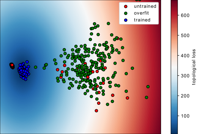
Figure 1: Shown above is a projection of what we refer to as the topological feature space of DNNs for a particular set of classification problems. Each point in this space denotes a network with its own set of parameters for a particular image classification task. This topological feature space effectively acts as a characterization of our hypothesis space. We see that regions in this space correspond to untrained, trained, and overfit models. In this work, we demonstrate the utility of such characterizations when they are computationally tractable. We not only show how we can achieve the goal of performance estimation without a testing set, but we can also infer the similarity between tasks and even construct meta-learning optimization strategies knowing the topological characteristics of learning.

The difficulty in analyzing mathematical objects like DNNs is not only due to the high number of parameters, but the complex graphical structure needed to operate on high dimensional data. Fortunately, tools rooted in algebraic topology have been developed to examine and compare sophisticated high-dimensional mathematical objects like manifolds and graphs [4]. The framework to examine persistent topological invariants is referred to as topological data analysis (TDA) and has shown to be an effective tool in understanding DNNs. Recent works have derived a set of features that effectively examine the underlying structure of DNNs that learn using TDA [5, 6, 7]. Corneau et al. for example showed that trained DNNs elicit particular topological features which differ from untrained DNNs, allowing us to address issues regarding their interpretability [5]. The general framework of these methods is to construct a mapping $G$ from a deep neural network $\mathcal{F}$ and training dataset $\mathbf{X}$, to topological features $\mathbf{t}$. The topological feature representation $\mathbf{t}$ is embedded in a space that we will refer to as the topological feature space. Given many model parameterizations and datasets, this topological feature space can be explored and used for tangible applications. For example, topological features can be used to accurately estimate the gap between training and testing performance [8].

Though the topological characterization proposed in [8] is effective in constructing a compressed representation that characterizes the progress of learning, it is difficult to use in practice due to computational complexity in terms of time and memory. Additionally, previously constructed topological characterizations are not readily equipped for backpropagation. This means that the DNN’s topological structure could not be explicitly modified using standard optimization strategies.

To solve the previous problems, we define a new class of topological features that characterize the progress of learning and can be easily computed at each training step. Additionally, our topological features are readily equipped for backpropagation. These two improvements result in major implications. We first demonstrate our topological characterization is still effectively estimating the performance of DNNs without the need for high-performance computing. Additionally, we show how our understanding of the topological feature space cannot only be used for performance estimation but for task-similarity estimation and meta-learning.

Our contributions are as follows 1) We define a new set of topological features, which characterize the topology of DNNs while being quick to compute at running time. This is especially useful when topological features of the network need to be analyzed at each iteration during training. 2) We show that these topological features are effective at estimating the testing performance without the need of a testing set. 3) We construct a mechanism to infer whether a model is appropriate for model selection given its representation in the topological feature space. 4) We construct an optimization strategy that enforces the topological consistencies of learning. This is shown to improve testing performance, even when training on small datasets.

2 Related Work

The sub-fields of meta-learning task similarity and general performance improvement for deep learning have been heavily explored in the machine learning community. For this work, however, we restrict ourselves to focusing on how topological data analysis has been applied in improving performance and understanding of DNNs.

Understanding DNNs with TDA: Topological data analysis (TDA) has demonstrated its use in understanding the topological differences between trained and untrained DNNs. [5] observed homological differences between trained and untrained deep networks when viewing the network as a clique complex, where connections between nodes are defined by the correlation in activations between them. Additionally, recent works observed similar results when viewing weight matrices of each layer in a neural network as a filtration (sequence of simplicial complexes) and performing persistent homology on the weight matrices to construct a stopping criterion [6]. Other works observed that the convolutions in deep networks elicit consistent topological structures when viewing each filter as a point in a higher-dimensional space [9].

These topological structures are so consistent that the testing error can be predicted as a function of them. In [8], the authors showed that the topological features induced by the correlation in activation between nodes can accurately predict testing error. Moreover, accurate predictions of the testing error were shown to be invariant across tasks, architectures, and datasets. Topological features induced from deep networks have also been used to determine whether networks have been fed adversarial samples [10, 5, 11].

Comparing DNNs with TDA for Task Similarity Examining a DNNs topological structure as a function of its training task has only been explored very recently. In [12], the authors construct a topological feature representation as a function of weight matrices and compare how the topological similarity varies with respect to change of task and change of model architecture. This work does not, however, show if the topological feature representation can be used for predicting task similarity.

Regularization and Model Selection with TDA: Recent works have developed methods that select model architectures as a function of the homology of the data itself. Intuitively, if the model cannot characterize the homology of the underlying dataset, the model certainly does not have the capacity to characterize the underlying structure of the data [13]. Network pruning methods have been constructed as a function of topological features. In [14] the authors first construct a filtration as a function of weight matrices. They then select weight values to be set to zero if those weight values correspond to certain homology classes within the filtration. In addition, other works have selected operators within the deep networks as a function of their topological properties [15]. Preserving topological information in images has shown to be useful in deep image segmentation problems [16, 17, 18]. Other works have applied differentiable frameworks which focus on the topology of the data being operated on. In [19] topological constraints in the latent space of an auto-encoder were introduced to obtain a more interpretable latent space. [20] applied topological constraints on the decision boundary of classifiers to mitigate overfitting. However, these methods only consider topological characteristics of the feature representation and do not consider the consistent topological features elicited by the networks themselves. Recently, frameworks have been developed to more conveniently induce specific topological features using gradient-based approaches [21]. Instead of merely characterizing networks topologically, we can actually enforce topological changes within the network using the conventional optimization strategies in neural network training.

3 Topological Preliminaries

Topological data analysis (TDA) characterizes the shape of the data using tools derived from algebraic topology. In this work, data is presented as a set of points $S$ on a manifold $M$. Given a set of points $S\subset M\subset\mathbb{R}^{d}$, we approximate the manifold by constructing a geometric simplicial complex $K_{\psi}(S)$, which is interpreted as a “triangulation” of our manifold M induced by S and a distance threshold $\psi$, where $\psi$ determines connections between points in S. A common topological feature extracted from $K_{\psi}(S)$ is its n-dimensional homology, and is often interpreted as characterizing the n-dimensional voids in $K_{\psi}(S)$. Since $K_{\psi}(S)$ changes with respect to the threshold $\psi$. It is of interest to see how the homology of $K_{\psi}(S)$ changes with respect to $\psi$. While varying the threshold $\psi$ we can construct a sequence of simplicial complexes known as a filtration $\mathbf{K}(S)$, where

$$\mathbf{K}(S):=\emptyset\subseteq K_{\psi_{1}}\subseteq K_{\psi_{2}}\subseteq K_{\psi_{3}}...$$ (1)

Using the filtration $\mathbf{K}(S)$ we record the thresholds $\psi_{i}$ where the n-dimensional homology changes in the filtration. For analysis, we consider the thresholds $\psi_{i}$ where n-dimensional voids are created or filled, also known as the birth and death of homology classes. The birth and death of a homology class is denoted as a persistence point $(\psi_{birth},\psi_{death})$. It is the collection of persistent points that are used to characterize the shape of our data. We note that our filtration constructions from DNNs differ greatly from previous works which may view DNNs as non-euclidean data. See [22] for rigorous definitions of abstract/ geometric simplicial complexes and persistent homology. Moreover, there are many classes of filtered complexes induced by point-sets. In this work, we examine the persistent homology of weak-alpha filtrations described by Bruel-Gabrielsson et al. [21]. We define $\mathbb{P}_{n}(S)$ as the set of persistent points corresponding to n-dimensional homology classes within our weak-alpha filtration $\mathbf{K}(S)$.

Many works have defined embeddings and similarity measures to analyze persistent points [23, 24, 25]. For this work, we simply compute statistics on the death of homology classes of $\mathbb{P}_{0}(S)$ to determine a topological characterization $t_{S}$ of $S$. Hence,

$$t_{S}=g(\mathbb{P}_{0}(S))$$ (2)

where $g$ is a differentiable function that computes statistics on persistence values. Such statistics include the maximum, minimum, mean, and standard deviation of $\mathbb{P}_{n}(S)$ Thus, $g(\mathbb{P}_{0}(S))$ is the operation that performs topological data analysis on $S$.

When incorporating topological features into a learning framework, it is of interest to understand how to differentiate elements of $t_{s}$ with respect to points in $S$. We use the optimization strategy defined in [21]. In [21], the derivative of topological features with respect to persistence values are equated to the derivative of topological features with respect to the pairs of points creating the persistence value. Hence given some topological statistic $t_{stat}$ and some threshold $\psi_{i}\in P_{0}(S)$,

$$\frac{\partial t_{stat}}{\partial\psi_{i}}=\frac{\partial t_{stat}}{\partial d^{pair}_{\psi_{i}}}$$ (3)

where $d^{pair}_{\psi_{i}}$ denotes the distance between the pair of points in $S$ that created the death of a homology class. Intuitively, increasing the persistence of a homology class is induced by making local increases to the distances between the pair of points that destroyed it.

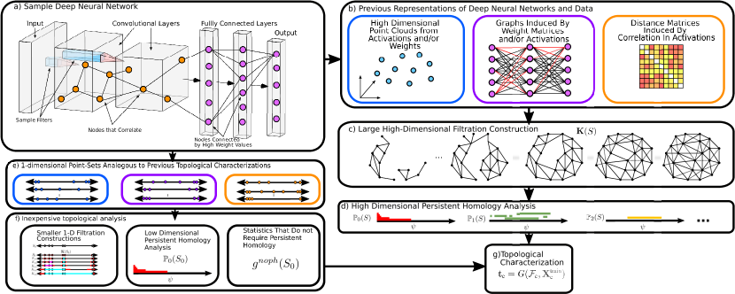
Figure 2: Shown above is a comparison between previous topological characterizations and ours, to provide some intuition for our filtration constructions. a) Given a particular deep neural network which in this case is a LeNet style architecture b) Previous works represent deep neural networks by first defining high dimensional point clouds, large graphs, or large distance matrices, each induced by weight matrices or activation values. c-d) However the previous works construct filtrations that are computationally expensive to construct and analyze the persistent homology of to ultimately construct a topological characterization $\mathbf{t}_{c}$ shown in g). e-f) In our work we construct a set of topological representations inspired by previous topological characterizations, but our topological characterizations are significantly less expensive computationally. This is because our topological characterizations operate on smaller 1-dimensional point-set representations of our deep neural network. Moreover, some of our operations do not require persistent homology analysis when producing $\mathbf{t}_{c}$.

4 Methods

Our first objective is to develop a topological characterization $\mathbf{t}_{\text{c}}$ of a DNN $\mathcal{F}_{\text{c}}$ trained for a particular classification task $\mathcal{T}_{\text{c}}$, where $c$ denotes the task. Hence, we aim to construct a differentiable mapping $G$ from our DNN and input data to our topological characterization of the network $\mathbf{t}_{c}$, i.e.

$$\mathbf{t}_{\text{c}}=G(\mathcal{F}_{\text{c}},\mathbf{X}^{\text{train}}_{\text{c}}).$$ (4)

We then show how to use this embedding function to construct a performance estimation strategy, task-similarity estimation strategy, and a meta-learning/knowledge transfer strategy.

4.1 Network Topology

We begin by defining the components of the network architecture, its parameters, and hidden feature representations of the DNN’s input data. We denote a set of labeled training data for task $\mathcal{T}_{\text{c}}$ as $D^{\text{train}}_{\text{c}}=\Big{\{}(X_{i},y_{i})\Big{\}}_{i=1}^{|D^{\text{train}}_{\text{c}}|}$, where $X_{i}\in\mathbb{R}^{|X_{\text{c}}|}$ is the sample input vector of size $|X_{\text{c}}|$, and $y_{i}\in\mathbb{N}$ denotes the sample label. When training a deep network, training samples are represented as a tensor; thus, we define $\mathbf{X}^{\text{ train}}_{\text{c}}\in\mathbb{R}^{n\times|X_{\text{c}}|}$ and $\mathbf{y}_{\text{c}}^{\text{train}}\in\mathbb{N}^{|D^{\text{train}}_{\text{c}}|}$ which concatenates all of the input training samples and training labels in $X^{\text{train}}_{\text{c}}$ into single tensors.

We denote our DNN $\mathcal{F}_{\text{c}}$ as a sequence of operators (layers) that iteratively transforms our input data $\mathbf{X}^{\text{train}}_{\text{c}}$ to find a representation that easily determines the class label. Thus,

$$\mathcal{F}_{\text{c}}(\mathbf{X}^{\text{train}}_{\text{c}})=f_{L}\circ...f_{2}\circ f_{1}(\mathbf{X}^{\text{train}}_{\text{c}})$$ (5)

or for a more convenient representation,

$$\mathcal{F}_{\text{c}}(\mathbf{X}^{\text{train}}_{\text{c}}):=\odot_{i=1}^{L}f_{i}(\mathbf{h_{i}}^{\text{train}}_{\text{c}})$$ (6)

where $\mathbf{h_{i}^{\text{train }}}\in\mathbb{R}^{|D^{\text{train}}_{\text{c}}|\times|h_{l}|}$, denoting the hidden feature representation of n samples each of size $|h_{i}|$ fed into layer $f_{i}$.

For now, and without loss of generalization, we assume all layers are fully connected layers, and we examine convolutional layers in the supplementary material.

We view the $i$-th fully connected layer of $\mathcal{F_{\text{c}}}$, $f_{i}$ as

$$\mathbf{h_{i+1}^{\text{train}}}=f_{i}(\mathbf{h_{i}^{\text{train}}})=\phi_{\text{ReLU}}(\mathbf{h_{i}^{\text{train}}}W_{i}\oplus b_{i})$$ (7)

equipped with a weight matrix $W_{l}\in\mathbb{R}^{|h_{i}|\times|h_{i+1}|}$, bias term $b_{i}\in\mathbb{R}^{|h_{l+1}|}$ and an element-wise activation function $\phi_{\text{ReLU}}$ which is a ReLU activation. $\oplus$ denotes a row-wise addition operator adding the bias term to the hidden feature representations of each sample. When considering a particular feature produced by layer $f_{i}$, we define $\mathbf{h_{i+1,j}^{\text{train }}}\in\mathbb{R}^{|D^{\text{train}}_{\text{c}}|}$ as the set of activations of the $j$-th column in $\mathbf{h_{i+1}^{\text{train }}}$ , also interpreted as the set of activations corresponding to the $j$-th node in the $i$+1-th layer of $\mathcal{F}_{\text{c}}$. We denote $w_{i,j,k}$ as the element in the $i$-th row and $j$-th column of $W_{i}$. We define the set of mean activations and standard deviation in activations of the $j$-th node in the $i$-th layer induced by $\mathbf{X}^{\text{train}}_{\text{c}}$ as $\mu^{\text{train}}_{i,j}$, $\sigma^{\text{train}}_{i,j}$ respectively.

4.2 Topological Characterization

Filtrations Induced by 1-Dimensional point-sets. Previous works topologically characterize DNNs by examining the higher-dimensional persistent homology of filtrations induced by distance matrices. However, the run-time to compute the persistence points corresponding to $n$-dimensional homology classes grows exponentially with respect to $n$ [8]. Moreover, constructing filtrations with the same number of points as nodes in an entire neural network is computationally expensive in both time and memory. To address this issue we define our own filtrations inspired by previous works in [5, 8, 10, 6, 26] which can be quickly computed. In addition, the features we compute are readily differentiable using methods described by Gabrielsson et al. [21]. Throughout our formulation of the framework, we will reference the previous works that inspired specific components of our topological characterization. Figure 2 provides some intuition relating previous topological characterizations and ours.

General Filtration Construction: To alleviate the run-time and memory usage we consider the following conditions for our topological characterization: 1) We consider constructing filtrations that only require a low-dimensional persistent homology analysis. 2) We view the DNN as a set of smaller filtrations as opposed to characterizing the DNN as one large filtration. 3) We consider feature representations inspired by previous topological characterizations which do not require persistent homology analysis.

We accomplish the first condition by viewing the network and data as a set of weak-alpha filtrations induced by point-sets residing in $\mathbb{R}$. Given that these point-sets only reside in one dimension, we only examine $\psi$ thresholds corresponding to the death of 0-dimensional homology classes. We then analyze the persistent homology of those weak-alpha filtrations and collect statistics on the persistence values to produce a topological characterization $\mathbf{t}_{\text{c}}$. Hence, given some point-set $S_{0}\subset\mathbb{R}$, we extract a topological characterization using our operation $t_{S_{0}}=g(\mathbb{P}_{0}(S_{0}))$. For convenience, we denote the following operation as $g^{ph}:=g(\mathbb{P}_{0})$.

To accomplish the second condition we consider the following framework to “break up” the DNN as a set of smaller filtrations. We propose a topological characterization that aims to capture the local, intermediate, and global topological properties of the DNNs that learn, encompassing many related works that study DNNs with TDA. We study the topology of scaled weight connections from each node to the next, statistics of hidden activations for each layer, and the covariance between nodes across multiple layers. The schematic of our function $G$ is shown in Figure 3. Depending on the size of our model $\mathcal{F}_{c}$, the classes of filtrations can be interchanged or removed to reduce the run time.

For the third condition, we examine statistics on the point-sets already provided by persistent homology analysis as this is already provided. Hence, we define $g^{noph}(S_{0})$ as a set of statistics computed on the point-set $S_{0}$ itself rather than statistics of persistent homology classes induced by $S_{0}$. These features can then be concatenated to define $g^{both}(S_{0})=[g^{ph}(S_{0}),g^{noph}(S_{0})]$. To be as general as possible with our future derivations, we define $\mathbf{g}$ to be a particular mapping chosen from $\{g^{ph},g^{noph},g^{both}\}$. We will see in our experiments how each class of topological characterization performs in various applications. See figure 3 for a diagram of our point-set representations and overall pipeline in constructing our mapping $G$.

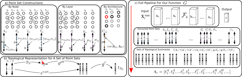
Figure 3: Schematic of how we topologically characterize the network. a) Here we show the classes of 1-dimensional point-sets extracted from the network, ranging from local to global structures inspired by previous works. b) From each of these point-sets we construct a topological characterization using our functions $g^{ph}$ and/or $g^{noph}$ along with $g^{\prime}$. c) We Show the full pipeline (top to bottom) to construct a topological characterization for a sample fully-connected network $\mathcal{F}_{c}$.

The Topology of Local Structures in the DNN: The first class of topological characterizations are defined to examine the local structures in our model $\mathcal{F}_{c}$. We are interested in examining the behavior of nodes in the network as they operate on data from one layer to the next. Inspired by [6], we construct 1-dimensional sets of points by considering the topology of weight values connected to a particular node in a single layer. We then scale these weight values by activation values like in [11] and [10]. As opposed to scaling the weight values by a single activation value, we scale the weight values by statistics of the hidden activations provided by the training data, as this reduces the number of filtrations being constructed. We consider the mean and standard deviation of actions corresponding to a single node. Consider the $j$-th node of the layer $f_{i}$ we define

$$A_{ij}=\{w_{ijk}\mu_{ij}|k\in 1...|h_{i+1}|\}$$ (8)

and

$$I_{ij}=\{\|w_{ijk}\sigma_{ij}\||k\in 1...|h_{i+1}|\}$$ (9)

where $\|\cdot\|$ denotes the absolute value. These point-sets will be used to topologically characterize one node’s contribution in manipulating the next hidden feature representation. Similarly, we define

$$A^{\prime}_{ij}=\{w_{ikj}\mu_{ik}|k\in 1...|h_{i}|\}$$ (10)

and

$$I^{\prime}_{ij}=\{\|w_{ikj}\sigma_{ij}\||k\in 1...|h_{i+1}|\}$$ (11)

which are used to topologically characterize how the nodes in the previous layer impact the activations of a particular node in the next layer. We then analyze the point-sets using our previously defined topological characterization. Hence, we define the following feature representations for the i-th layer,

$$\mathbb{T}(\mathbf{A}_{i})=\{\mathbf{g}(A_{i1}),\mathbf{g}(A_{i2})...\}$$ (12)

$$\mathbb{T}(\mathbf{A^{\prime}}_{i})=\{\mathbf{g}(A^{\prime}_{i1}),\mathbf{g}(A^{\prime}_{i2})...\}$$ (13)

$$\mathbb{T}(\mathbf{I}_{i})=\{\mathbf{g}(I_{i1}),\mathbf{g}(I_{l2})...\}$$ (14)

$$\mathbb{T}(\mathbf{I^{\prime}}_{i})=\{\mathbf{g}(I^{\prime}_{i1}),\mathbf{g}(I^{\prime}_{i2})...\}$$ (15)

Topological Structures Induced by Layers: As previously discussed, recent works have constructed characterizations at higher resolutions by examining the topological structures induced by the entire layer. To topologically characterize the entire layer we propose our own topological characterizations. We first randomly select weights from the weight matrix and scale them by their corresponding mean activations. Thus, for a single point-set,

$$A^{\prime\prime}_{il}=\{w_{ijk}\mu_{ij}|j\in J_{l},k\in K_{l}\}$$ (16)

$$I^{\prime\prime}_{il}=\{||w_{ijk}\sigma_{ij}|||i\in J_{l},j\in J_{l}\}$$ (17)

Where $J_{l}$ and $K_{l}$ are a set of randomly selected indices. We then compute the same topological feature representation as we did for the single node, hence

$$\mathbb{T}(\mathbf{A^{\prime\prime}}_{i})=\{\mathbf{g}(A^{\prime\prime}_{i1}),\mathbf{g}(A^{\prime\prime}_{i2})...\}$$ (18)

$$\mathbb{T}(\mathbf{I^{\prime\prime}}_{i})=\{\mathbf{g}(I^{\prime\prime}_{i1}),\mathbf{g}(I^{\prime\prime}_{i2})...\}$$ (19)

We also consider the topological characteristics of the hidden activations for each layer. Similar to [26] we consider a lower-dimensional characterization of hidden activation values as data passes through the network. However, we simply consider statistics in the activation values.

$$H_{\sigma_{i}}=\{\sigma_{ij}|j\in 1...|h_{i}|\},$$ (20)

and

$$H_{\mu_{i}}=\{\mu_{ij}|j\in...|h_{i}|\}$$ (21)

where the topological feature representation is

$$t^{H}_{i}=[\mathbf{g}(H_{\mu_{i}}),\mathbf{g}(H_{\sigma_{i}})].$$ (22)

Topological Structures Induced by the Entire Architecture To examine the global topological structure of the DNN, we consider the covariance in activations between nodes across multiple layers. Though a Rips-Filtration can be induced by distance matrices which are a function of covariance matrices like in [5] and [8], we drastically reduce the run time by considering the topology of point-sets induced by the covariance in activations between one node with respect to the activations of other nodes in the network. Given the set of activations for the j-th node in the i-th layer $\mathbf{h_{ij}}$, we define $C_{ij}$ as a set of covariance values between the $j$-th node in the $i$-th layer the activations from a set of nodes selected throughout the DNN. Thus

$$C_{ij}=\{cov(\mathbf{h}_{ij},\mathbf{h}_{k})|k\in\mathcal{C}_{ij}^{\text{ind}}\},$$ (23)

where $\mathcal{C}_{ij}^{\text{ind}}$ denotes a set of indices corresponding to nodes throughout the network. Thus for the i-th layer in the network

$$\mathbb{T}(\mathbf{C}_{i})=\{\mathbf{g}(C_{i1}),\mathbf{g}(C_{i2})...\}.$$ (24)

Aggregating Persistence Point Statistics into One Topological Feature Since we broke up our DNN $\mathcal{F}_{c}$ into a set of simplicial complexes at each layer, we need to ensure that our topological features are permutation invariant. This is addressed by applying an additional set of statistics on our topological summaries. Similar to our function $g$, we denote $g^{\prime}$ as a differentiable function which computes the mean and standard deviation of our sets of topological summaries. Thus for the $i$-th layer we have the following feature representations:

$$t^{\text{A}}_{i}=[g^{\prime}(\mathbb{T}(\mathbf{A}_{i})),g^{\prime}(\mathbb{T}(\mathbf{A^{\prime}}_{i})),g^{\prime}(\mathbb{T}(\mathbf{A^{\prime\prime}}_{i}))],$$ (25)

$$t^{\text{I}}_{i}=[g^{\prime}(\mathbb{T}(\mathbf{I}_{i})),g^{\prime}(\mathbb{T}(\mathbf{I^{\prime}}_{i})),g^{\prime}(\mathbb{T}(\mathbf{I^{\prime\prime}}_{i}))],$$ (26)

$$t^{\text{C}}_{i}=[g^{\prime}(\mathbb{T}(\mathbf{C}_{i}))]$$ (27)

We then combine all of our topological features into one vector for our final topological representation

$$\mathbf{t}_{c}=[t^{A}_{1},t^{A}_{2},...t^{I}_{1},t^{I}_{2},...t^{C}_{1},t^{C}_{2},...,t^{H}_{1},t^{H}_{2},...].$$ (28)

We define $G$ as the set of previously described operations that result in our topological representation $\mathbf{t}_{c}$. Since our topological feature representation is constructed using simplicial complexes equipped with gradients as described in [21], and the statistics we compute using g and g’ are differentiable, we know that the composition of our differentiable functions $G$ is also differentiable. Therefore, we are equipped to enforce the network to elicit particular topological structures using conventional gradient-based optimization strategies.

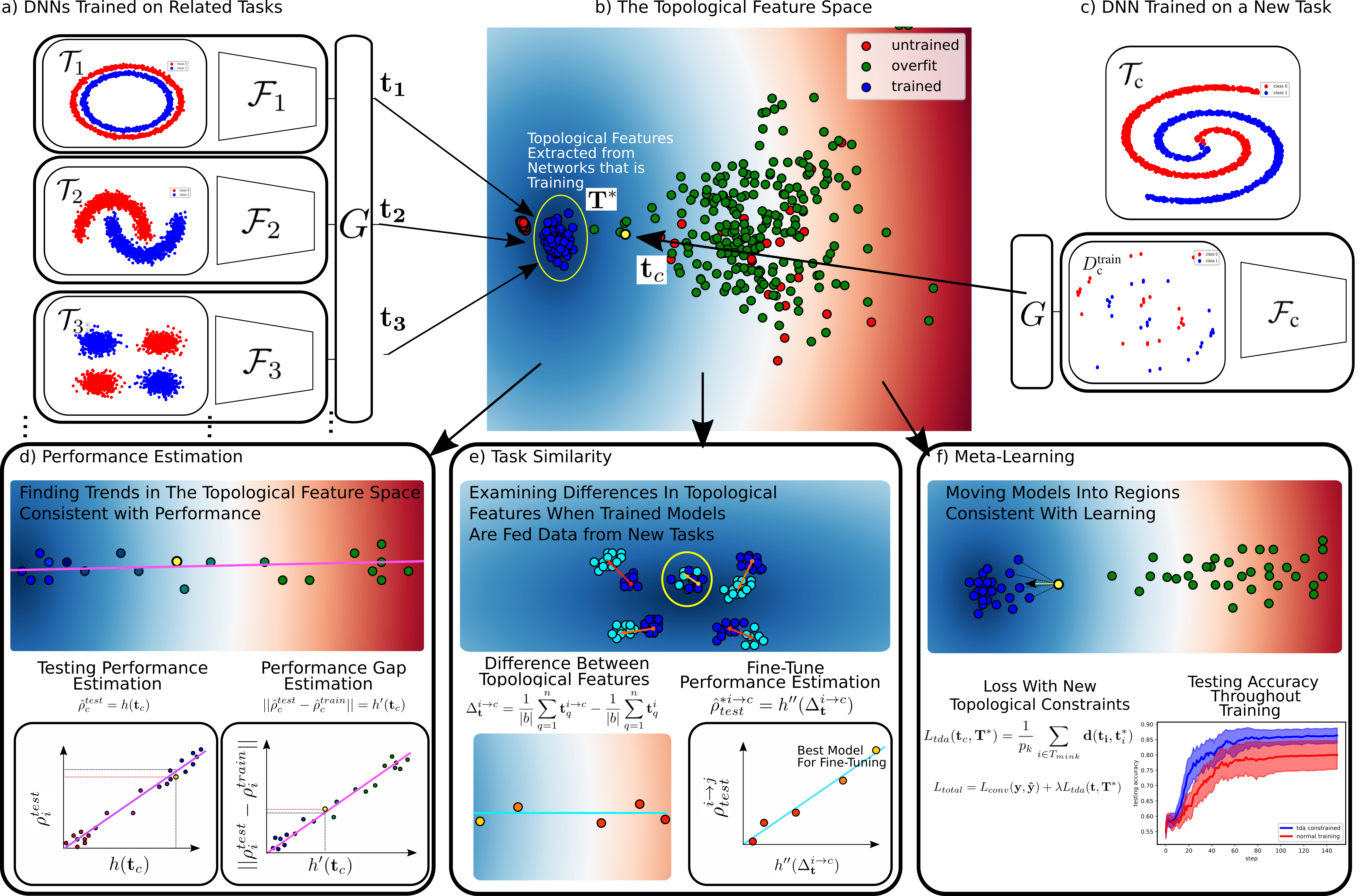
Figure 4: Here we show how we leverage our understanding of the topological feature space a) Shows a set of DNNs trained on a set of tasks where training data was abundant. b) From these trained deep networks and tasks, we extract topological features with our function mapping $G$ and use the topological features $\mathbf{T^{*}}$ induced from networks we know achieve a high classification accuracy. c) Shows a new classification task where data is not as abundant with a DNN currently being trained. d) We can first analyze the topological feature to estimate our testing performance for our model $\mathcal{F}_{c}$ using our training set only. e) We can also feed our previously trained models our training data from $\mathcal{T}_{c}$ and estimate the fine-tuning testing performance. This allows us to infer task similarity by determining the pre-trained model with the highest estimated testing performance. f) Lastly, we can ”pull” models into regions consistent with learning within the topological feature space and find that it can consistently improve testing performance for many different classification problems.

5 Applications

We first verify our new topological features are capable of performing tasks explored by previous works which study deep networks with TDA. One task, in particular, is the ability to discriminate between trained and overfit models. Next, we show that our topological features are effective in estimating the testing performance and performance gap (difference between training and testing performance) of models that have been trained. We then demonstrate how these topological features can be used for pre-trained model selection to achieve a higher testing performance after fine-tuning as this effectively determines if two tasks are related to each other. Lastly, we develop a meta-learning strategy to enforce the topological characteristics consisting with learning, that is, we explicitly enforce networks to have similar topological structures to networks successfully trained on different tasks. All applications are shown in figure 4.

5.1 Performance Estimation

For each performance estimation experiment, we have gathered a set of topological features induced by models trained across a set of tasks. For a given classification task, we compute topological features $\mathbf{t}_{i}$, their intended model state $m^{state}_{i}$ (whether the model is untrained, trained with sufficient data, or trained with insufficient data), and training and testing accuracies $\rho^{train}_{i},\rho^{test}_{i}$ respectively. Note that this does not include topological features induced from our a testing current task $\mathcal{T}_{c}$.

$$D^{meta}_{top}=\{(\mathbf{t}_{i},m^{state}_{i},\rho^{train}_{i},\rho^{test}_{i})\}_{i=1}^{|D_{top}|}.$$ (29)

Distinguishing Between Model States We explore the space where our topological features reside to determine the regions within the topological space that correspond to networks that learn. This is done by predicting the intended model states of topological features $\mathcal{T}_{c}$ using a k-nearest neighbor classifier $\mathbb{NN}_{k}$ trained with standardized samples $\mathbf{t}_{i}$ and labels $m^{state}_{i}$ defined in (29). Hence,

$$\widehat{m}^{state}_{c}=\mathbb{NN}_{k}(\mathbf{t}_{c}).$$ (30)

where $\widehat{m}^{state}_{c}$ denotes the predicted model state induced by the k-nearest neighbor classifier.

Estimating Testing Performance To estimate the testing performance we construct a linear model

$$\hat{\rho}^{test}_{c}=h(\mathbf{t}_{c})=\mathbf{\beta}_{h}^{T}\mathbf{t}_{c}+\beta_{h0},$$ (31)

where $\mathbf{\beta}_{h}\in\mathbb{R}^{|\mathbf{t}_{c}|}$ and $\beta_{h0}\in\mathbb{R}$ denote the linear model parameters, and $\hat{\rho}^{test}_{c}$ denotes the estimated testing accuracy. Our linear model fitted using all topological features $\mathbf{t}_{i}$ and testing performancea $\rho^{test}_{i}$ from $D^{meta}_{top}$ where the training accuracy is above a threshold. We fit our model $h$ by minimizing the mean square error (MSE) with an L1-regularizer (LASSO Regression).

Estimating Performance Gap Similarly, we construct another LASSO model to estimate the performance gap where

$$||\hat{\rho}^{test}_{c}-\hat{\rho}^{train}_{c}||=h^{\prime}(\mathbf{t}_{c})=\mathbf{\beta}_{h^{\prime}}^{T}\mathbf{t}_{c}+\beta_{h^{\prime}0},$$ (32)

where is $h^{\prime}$ is a linear model fitted using topological features $\mathbf{t_{i}}$, and performance gap $||\rho^{test}_{i}-\rho^{train}_{i}||$ from $D^{meta}_{top}$, in which the training accuracy is above a threshold. $\mathbf{\beta}_{h^{\prime}}$ and $\beta_{h^{\prime}0}$ denote the linear model parameters for $h^{\prime}$.

5.2 Task Similarity Estimation For Pre-trained Model Selection

Upon further exploration of this topological feature space, we have found that pre-trained models differ topologically when they are fed training data corresponding to different tasks. This has raised the question as to whether we can use this “topological disparity” to determine if a pre-trained model is appropriate for a given task. In this application we assume we have a bank of models $\mathbfcal{F}_{s}=\{\mathcal{F}_{1},\mathcal{F}_{2},\mathcal{F}_{3}...\}$ trained on on a set of tasks with corresponding training datasets $\mathbf{X}_{s}=\{\mathbf{X}_{1},\mathbf{X}_{2},\mathbf{X}_{3}...\}$. Given our new task $\mathcal{T}_{c}$ with a set of training samples $\mathbf{X}_{c}$, we could train a new network $\mathcal{F}_{c}$ using our current training set $\mathbf{X}_{c}$; however, it may be of interest to simply select a pre-trained model from $\mathbfcal{F}_{s}$ that is trained on a task related to $\mathcal{T}_{c}$. Moreover, instead of immediately training a whole set of pre-trained models in $\mathbfcal{F}_{s}$ to determine which model is best suited for $\mathcal{T}_{c}$, we can first examine the topological features induced by each of the models as this is computationally less expensive and does not require a testing set for $\mathcal{T}_{c}$ .

We can construct the following topological feature representations that feeds our current data into the previously defined models, hence $\mathbf{t}^{i\rightarrow c}=\mathbf{G}(\mathcal{F}_{i},\mathbf{X}_{c})$, where $\mathbf{t}^{i\rightarrow c}$ denotes the topological features induced by feeding model $\mathcal{F}_{i}$, our current dataset $\mathbf{X}_{c}$. We formulate the problem of inferring task similarity selecting the most appropriate model $\mathcal{F}_{i}$ for fine-tuning. Hence we desire a model $H$ which performs the following operation

$$i^{*}=H({X_{c},\mathbf{X}_{s},\mathbfcal{F}_{s})},$$ (33)

Where $i^{*}$ denotes the index corresponding to the most appropriate model in $\mathbfcal{F}_{s}$ for task $\mathcal{T}_{c}$.

One might ask how we determine the model that is most appropriate for fine-tuning. The proxy we use to infer task-simlarity is simply an estimation of the fine-tuning testing performance for a given pre-trained model. Similar to our previous models which estimate the testing performance and performance gap, we estimate the fine-tuning testing performance of a given model as a function of topological features. However, unlike the topological features derived in our previous models, we examine the difference between topological feature representations.

Suppose we have a set of $|b|$ topological features corresponding to $|b|$ different training batches fed into a model trained on task $\mathcal{T}_{i}$. We first compute the average difference between topological features induced by models fed data they were previously trained on and data corresponding to the current tasks. Hence

$$\Delta_{\mathbf{t}}^{i\rightarrow c}=\frac{1}{|b|}\sum_{q=1}^{n}\mathbf{t}^{i\rightarrow c}_{q}-\frac{1}{|b|}\sum_{q=1}^{n}\mathbf{t}^{i}_{q}$$ (34)

We then use $\Delta_{\mathbf{t}}^{i\rightarrow c}$ to estimate the testing performance of $\mathcal{F}_{i}$ on task $\mathcal{T}_{c}$ after fine-tuning.

Like the previous performance estimation methods, we construct a lasso linear model as a function of our topological difference to estimate the average final testing performance of the fine-tuned model.

$$\hat{\rho}^{*i\rightarrow c}_{test}=h^{\prime\prime}(\Delta_{\mathbf{t}}^{i\rightarrow c})=\beta^{T}_{h^{\prime\prime}}\Delta_{\mathbf{t}}^{i\rightarrow c}+\beta_{h0^{\prime\prime}}$$ (35)

Where $\hat{\rho}^{*i\rightarrow c}_{test}$ denotes the expected final testing performance after fine-tuning models on task $\mathcal{T}_{c}$ which were pre-trained on $\mathcal{T}_{i}$. Finally, our model selection is defined to be

$$i^{*}=\operatorname*{arg\,max}_{i}h^{\prime\prime}(\Delta_{\mathbf{t}}^{i\rightarrow c})$$ (36)

When training our model $h^{\prime\prime}$ we use the the following dataset

$$D_{top}^{meta-sim}=\{(\rho^{i\rightarrow j}_{test},\Delta_{\mathbf{t}}^{i\rightarrow j})\}_{i,j\neq c}$$ (37)

not including any data corresponding to task $\mathcal{T}_{c}$

5.3 Meta-Learning Strategy

During conventional training we define a loss function $L_{conv}(\mathcal{F}_{\text{c}}(\mathbf{X}^{\textbf{train}}_{\textbf{c}}),\mathbf{y}_{\text{c}}^{\text{train}})$ that is a function of the DNN’s output and labeled training data. We aim to improve the testing performance of $\mathcal{F}_{\text{c}}$ by “pulling” our DNN into regions within the topological feature space that are consistent with learning (See Figure 4). This is accomplished by minimizing the distance between our current topological features $\mathbf{t}_{c}$ and the topological features we know to be consistent with learning. Suppose we select a set of topological features $\mathbf{T^{*}}$ from $D^{meta}_{top}$ induced from other DNNs we know perform well on various tasks in terms of their testing accuracy.

$$\mathbf{T^{*}}=\{\mathbf{t}^{*}_{i}\}_{i=1}^{|T*|}=\{\mathbf{t}_{i}\in D^{meta}_{top}|\rho^{test}_{i}>\rho_{\text{thresh}}\}$$ (38)

We construct a topological loss by selecting the $p_{k}$ nearest topological features with respect to $\mathbf{t}_{c}$ from a random sample of $\mathbf{T^{*}}$ selected at each training set. Thus,

$$L_{tda}(\mathbf{t}_{c},\mathbf{T^{*}})=\frac{1}{p_{k}}\sum_{i\in T_{mink}}\mathbf{d}(\mathbf{t_{c}},{\mathbf{t}}^{*}_{i})$$ (39)

where $T_{mink}$ is the set of indices denoting the closest $p_{k}$ topological features $\mathbf{t}$ in a random sub-sample of $\mathbf{T}^{*}$, and $\mathbf{d}(\cdot,\cdot)$ denotes a weighted euclidean distance between $\mathbf{t_{c}}$ and $\mathbf{t_{i}^{*}}$. We determine weighting by first standardizing the features according to $D^{meta}_{top}$ and selecting components of the topological features that correlate with testing performance. More formally,

$$d(\mathbf{t_{c}},\mathbf{t}^{*}_{i})=\frac{1}{|\mathbf{t}|}\sum_{j=1}^{|\mathbf{t}|}\frac{\mathbf{1}_{j}||t_{cj}-t^{*}_{ij}||}{\sigma_{j}}$$ (40)

where $t_{cj}$ and $t^{*}_{ij}$ denote the components of $\mathbf{t_{c}}$ and $\mathbf{t}^{*}_{i}$ respectively, $\sigma_{j}$ denotes the standard deviation of the $j$-th topological feature component in $D^{meta}_{top}$ , and

$$\mathbf{1}_{j}=\begin{cases}1,&||corr(\mathbf{t}^{j},\mathbf{p}^{test})||\geq\tau_{corr}\\ 0,&||corr(\mathbf{t}^{j},\mathbf{p}^{test})||<\tau_{corr}\end{cases}$$ (41)

where $corr(\mathbf{t}^{j},\mathbf{p}^{test})$ denote the pearson correlation between the $j$-th topological feature component in and the corresponding testing accuracy estimated in $D^{top}_{meta}$ and $\tau_{corr}$ is a threshold. When training we consider the following loss function

$$L_{total}=L_{conv}(\mathbf{y}^{\text{train}}_{c},\widehat{\mathbf{y}}^{\text{train}}_{c})+\lambda L_{tda}(\mathbf{t}_{c},\mathbf{T^{*}}),$$ (42)

where $\lambda$ is an additional hyperparameter.

6 Experiments

6.1 Dataset Construction

We gather topological features across mutually exclusive classification problems. We define 3 classes of parent datasets used in the experiments: synthetic 2-dimensional data, greyscale image data, and downsampled ImageNet data.

Synthetic 2-dimensional datasets: Our synthetic 2-dimensional datasets consist of a set of binary classification problems generated from the scikit learn database [27]. Such datasets include discriminating between samples that resemble spirals, moons, circles, and Gaussian distributed data. For each classification problem, we generate 4000 training and testing samples for each binary classification problem. To have more diversity in our datasets, we apply a series of augmentations like rotations and non-isotropic scaling to each generated 2D dataset. We assume the augmentations result in the different classification problems for the performance estimation experiments. However, for the task-similarity and meta-learning experiments, we do not include augmented datasets when fitting $h^{\prime\prime}$ or selecting $\mathbf{T}^{*}$.

greyscale Image datasets: We also consider greyscale image classification problems. We combine MNIST [28], KMNIST [29] and EMNIST [30] datasets. This aggregation would have a total number of 46 classes. We randomly partition each of the grey image datasets into groups of $m\in 2,4,\text{and }8$. This means, that we randomly select m classes from the augmented dataset to test the applications in Section 5 and the rest of the classes are used for generating topological features for training our meta-learning applications. We state the specific class partitioning in the supplementary material. Note that when we split the data, we maintain the initial partitioning of training and testing samples for each class as defined by previous works.

Downsampled Imagenet Data: We also use a downsampled version of ImageNet known as Tiny-Imagenet [31] consisting of 200 classes of colored images. Image classes are randomly partitioned into groups of 2 such that we have 100 2-class problems. Samples belonging to the original training and testing sets remain as defined by previous works. Both image samples are standardized by pixel intensity. Specific class partitions are defined in the supplementary material.

6.2 Models

For synthetic 2D classification problems, we trained networks with fully connected layers each equipped with 25 hidden units with ReLu activation functions. For the greyscale and downsampled ImageNet datasets, models are equipped with a LeNet style architecture. The models first begin with convolution layers, equipped ReLU activations, and with max pooling. After the convolution layers, two fully connected layers are applied. See Table I which defines the list of architectures used for our performance estimation and meta-learning strategy.

Model Name Model Operation Sequence synth fc6 $\text{In}\rightarrow(\text{FC-25}\rightarrow\text{Relu})_{\times 5}\rightarrow\text{FC-NC}\rightarrow\text{Out}$ synth fc8 $\text{In}\rightarrow(\text{FC-25}\rightarrow\text{Relu})_{\times 7}\rightarrow\text{FC-NC}\rightarrow\text{Out}$ synth fc10 $\text{In}\rightarrow(\text{FC-25}\rightarrow\text{Relu})_{\times 9}\rightarrow\text{FC-NC}\rightarrow\text{Out}$ gconv2 $\text{In}\rightarrow(\text{Conv3x3-8}\rightarrow\text{Relu}\rightarrow\text{MaxPool2x2})_{\times 2}\rightarrow$ $\text{FC-50}\rightarrow\text{Relu}\rightarrow\text{FC-NC}\rightarrow\text{Out}$ gconv3 $\text{In}\rightarrow(\text{Conv3x3-8}\rightarrow\text{Relu}\rightarrow\text{MaxPool2x2})_{\times 3}\rightarrow$ $\text{FC-50}\rightarrow\text{Relu}\rightarrow\text{FC-Nc}\rightarrow\text{Out}$ gconv4 $\text{In}\rightarrow(\text{Conv3x3-8}\rightarrow\text{Relu}\rightarrow\text{MaxPool2x2})_{\times 2}\rightarrow(\text{Conv3x3-64}\rightarrow\text{Relu})_{\times 2}\rightarrow$ $\text{FC-50}\rightarrow\text{Relu}\rightarrow\text{FC-NC}\rightarrow\text{Out}$ tconv3 $\text{In}\rightarrow(\text{Conv3x3-8}\rightarrow\text{Relu}\rightarrow\text{MaxPool2x2})_{\times 3}\rightarrow\text{Conv3x3-16}\rightarrow\text{Relu}\rightarrow\text{MaxPool2x2}\rightarrow$ $\text{FC-50}\rightarrow\text{Relu}\rightarrow\text{FC-NC}\rightarrow\text{Out}$ tconv4 $\text{In}\rightarrow(\text{Conv3x3-8}\rightarrow\text{Relu}\rightarrow\text{MaxPool2x2})_{\times 2}\rightarrow\text{Conv3x3-16}\rightarrow\text{Relu}\rightarrow\text{MaxPool2x2}\rightarrow\text{Conv3x3-16}\rightarrow\text{Relu}\rightarrow$ $\text{FC-120}\rightarrow\text{Relu}\rightarrow\text{FC-NC}\rightarrow\text{Out}$ tconv5 $\text{In}\rightarrow(\text{Conv3x3-8}\rightarrow\text{Relu}\rightarrow\text{MaxPool2x2})_{\times 2}\rightarrow\text{Conv3x3-16}\rightarrow\text{Relu}\rightarrow\text{MaxPool2x2}$ $\rightarrow(\text{Conv3x3-16}\rightarrow\text{Relu})_{\times 2}\rightarrow$ $\text{FC-120}\rightarrow\text{Relu}\rightarrow\text{FC-NC}\rightarrow\text{Out}$

TABLE I: List of architectures used in our experiments. Models are denoted as a sequence of operations from left to right where each operation is denoted between arrows $\rightarrow$. FC and Conv, MaxPool, and Relu denote fully-connected Layers, 2D-convolutional layers, max pooling layers and ReLu activation functions respectively. Each convolutional layer denotes the filter patch size as well as the number of filters used in each layer. For example, Conv3x3-8 denotes a convolutional layer equipped with 8 filters each filter being of 3x3. Similarly, MaxPool2x2 denotes a Max Pooling Layer with a kernel size of 2x2. FC-# denotes a fully connected layer whose output representation is of size # (NC denotes the number of classes for the particular classification problem).In and Out denote the input and output tensors respectively._# denotes a repetition of a sequence of operations. For example $(\text{FC-25}\rightarrow\text{Relu})_{\times 5}$ would consist of a sequence of 5 fully-connected layers where each layer is equipped with a ReLU activation function.

	Testing Performance Estimation
Synthetic	Model State			Testing Acc			Performance Gap
2D-Data	Mean Acc (%)			MAE (%)			MAE (%)
Model	$g^{ph}$	$g^{noph}$	$g^{both}$	$g^{ph}$	$g^{noph}$	$g^{both}$	$g^{ph}$	$g^{noph}$	$g^{both}$
synth fc6	84.67 $\pm$ 2.79	88.33 $\pm$ 2.49	88.44 $\pm$ 2.67	5.04 $\pm$ 2.79	5.11 $\pm$ 2.49	4.97 $\pm$ 2.67	5.16 $\pm$ 0.65	5.11 $\pm$ 0.63	5.08 $\pm$ 0.62
synth fc8	79.78 $\pm$ 3.06	83.00 $\pm$ 2.72	82.56 $\pm$ 2.94	5.10 $\pm$ 3.06	5.11 $\pm$ 2.72	4.90 $\pm$ 2.94	5.24 $\pm$ 0.62	5.15 $\pm$ 0.59	4.99 $\pm$ 0.59
synth fc10	82.89 $\pm$ 2.65	87.00 $\pm$ 1.85	87.33 $\pm$ 2.00	4.98 $\pm$ 2.65	4.89 $\pm$ 1.85	4.88 $\pm$ 2.00	4.98 $\pm$ 0.51	4.86 $\pm$ 0.51	4.87 $\pm$ 0.51
Grey 2	Model State			Testing Acc			Performance Gap
Data	Mean Acc (%)			MAE (%)			MAE (%)
Model	$g^{ph}$	$g^{noph}$	$g^{both}$	$g^{ph}$	$g^{noph}$	$g^{both}$	$g^{ph}$	$g^{noph}$	$g^{both}$
gconv2	99.86 $\pm$ 0.14	99.86 $\pm$ 0.14	99.86 $\pm$ 0.14	3.65 $\pm$ 0.14	3.61 $\pm$ 0.14	3.62 $\pm$ 0.14	3.49 $\pm$ 0.28	3.45 $\pm$ 0.27	3.45 $\pm$ 0.27
gconv3	99.71 $\pm$ 0.20	99.71 $\pm$ 0.20	99.71 $\pm$ 0.20	3.60 $\pm$ 0.20	3.53 $\pm$ 0.20	3.54 $\pm$ 0.20	3.60 $\pm$ 0.37	3.49 $\pm$ 0.35	3.50 $\pm$ 0.35
gconv4	99.57 $\pm$ 0.23	99.71 $\pm$ 0.20	99.71 $\pm$ 0.20	4.07 $\pm$ 0.23	3.84 $\pm$ 0.20	3.85 $\pm$ 0.20	3.77 $\pm$ 0.33	3.49 $\pm$ 0.31	3.49 $\pm$ 0.31
Grey 4	Model State			Testing Acc			Performance Gap
Data	Mean Acc (%)			MAE (%)			MAE (%)
Model	$g^{ph}$	$g^{noph}$	$g^{both}$	$g^{ph}$	$g^{noph}$	$g^{both}$	$g^{ph}$	$g^{noph}$	$g^{both}$
gconv2	100.00 $\pm$ 0.00	100.00 $\pm$ 0.00	100.00 $\pm$ 0.00	4.98 $\pm$ 0. 00	5.04 $\pm$ 0.00	5.06 $\pm$ 0.00	4.19 $\pm$ 0.63	3.37 $\pm$ 0.48	3.37 $\pm$ 0.48
gconv3	100.00 $\pm$ 0.00	99.70 $\pm$ 0.29	100.00 $\pm$ 0.00	4.19 $\pm$ 0.0 0	3.72 $\pm$ 0.29	3.69 $\pm$ 0.00	4.28 $\pm$ 0.65	3.56 $\pm$ 0.33	3.52 $\pm$ 0.34
gconv4	100.00 $\pm$ 0.00	100.00 $\pm$ 0.00	100.00 $\pm$ 0.00	4.35 $\pm$ 0. 00	4.23 $\pm$ 0.00	4.29 $\pm$ 0.00	4.11 $\pm$ 0.58	3.73 $\pm$ 0.50	3.77 $\pm$ 0.50
Grey 8	Model State			Testing Acc			Performance Gap
Data	Mean Acc (%)			MAE (%)			MAE (%)
Model	$g^{ph}$	$g^{noph}$	$g^{both}$	$g^{ph}$	$g^{noph}$	$g^{both}$	$g^{ph}$	$g^{noph}$	$g^{both}$
gconv2	100.00 $\pm$ 0.00	100.00 $\pm$ 0.00	100.00 $\pm$ 0.00	4.60 $\pm$ 0. 00	3.77 $\pm$ 0.00	3.85 $\pm$ 0.00	4.55 $\pm$ 1.14	3.90 $\pm$ 0.99	3.94 $\pm$ 0.9
gconv3	100.00 $\pm$ 0.00	99.33 $\pm$ 0.60	100.00 $\pm$ 0.00	3.59 $\pm$ 0.0 0	3.66 $\pm$ 0.60	3.68 $\pm$ 0.00	3.85 $\pm$ 0.96	4.05 $\pm$ 0.78	4.01 $\pm$ 0.78
gconv4	99.33 $\pm$ 0.60	100.00 $\pm$ 0.00	99.33 $\pm$ 0.60	4.70 $\pm$ 0.60	3.44 $\pm$ 0.00	3.66 $\pm$ 0.60	4.63 $\pm$ 0.86	3.41 $\pm$ 0.66	3.57 $\pm$ 0.66
Tiny 2	Model State			Testing Acc			Performance Gap
Data	Mean Acc (%)			MAE (%)			MAE (%)
Model	$g^{ph}$	$g^{noph}$	$g^{both}$	$g^{ph}$	$g^{noph}$	$g^{both}$	$g^{ph}$	$g^{noph}$	$g^{both}$
tconv3	97.67 $\pm$ 0.35	98.80 $\pm$ 0.23	98.43 $\pm$ 0.26	6.66 $\pm$ 0.35	6.57 $\pm$ 0.23	6.60 $\pm$ 0.26	6.01 $\pm$ 0.30	5.76 $\pm$ 0.29	5.76 $\pm$ 0.29
tconv4	95.90 $\pm$ 0.51	97.87 $\pm$ 0.34	97.20 $\pm$ 0.43	7.26 $\pm$ 0.51	7.12 $\pm$ 0.34	7.10 $\pm$ 0.43	6.88 $\pm$ 0.38	6.49 $\pm$ 0.36	6.49 $\pm$ 0.36
tconv5	95.90 $\pm$ 0.45	97.53 $\pm$ 0.33	97.30 $\pm$ 0.33	7.42 $\pm$ 0.45	7.09 $\pm$ 0.33	7.02 $\pm$ 0.33	7.06 $\pm$ 0.39	6.62 $\pm$ 0.36	6.59 $\pm$ 0.36

TABLE II: Performance Estimation Results. The first 3 columns denote the average classification accuracy ( $\pm$ standard error) in predicting the intended model state using $\mathbb{NN}_{k}$ . The next 6 columns present the mean absolute error in % $\pm$ the standard error in estimating the testing accuracy and performance gap respectively using $h$ and $h^{\prime}$. $g^{ph}$,$g^{noph}$, and $g^{both}$ refer the particular topological characterization selected.

	Task Similarity
Synthetic	Model Rank			Corr			Testing Improvement
2D-Data	–			–			(%)
$n_{models}=5$	$g^{ph}$	$g^{noph}$	$g^{both}$	$g^{ph}$	$g^{noph}$	$g^{both}$	$g^{ph}$	$g^{noph}$	$g^{both}$
synth fc6	2.00 $\pm$ 0.28	1.60 $\pm$ 0.36	1.60 $\pm$ 0.36	0.41 $\pm$ 0.26	0.52 $\pm$ 0.26	0.51 $\pm$ 0.25	2.59 $\pm$ 1.66	4.07 $\pm$ 1.77	4.07 $\pm$ 1.77
synth fc8	1.80 $\pm$ 0.44	1.40 $\pm$ 0.36	1.80 $\pm$ 0.44	0.46 $\pm$ 0.24	0.69 $\pm$ 0.15	0.68 $\pm$ 0.15	3.68 $\pm$ 1.79	4.21 $\pm$ 1.67	3.68 $\pm$ 1.79
synth fc10	2.20 $\pm$ 0.33	1.20 $\pm$ 0.18	1.20 $\pm$ 0.18	0.65 $\pm$ 0.08	0.87 $\pm$ 0.06	0.88 $\pm$ 0.03	2.96 $\pm$ 2.41	5.64 $\pm$ 1.68	5.64 $\pm$ 1.68
Grey 2	Model Rank			Corr			Testing Improvement
2D-Data	–			–			(%)
$n_{models}=22$	$g^{ph}$	$g^{noph}$	$g^{both}$	$g^{ph}$	$g^{noph}$	$g^{both}$	$g^{ph}$	$g^{noph}$	$g^{both}$
gconv2	7.22 $\pm$ 1.04	7.61 $\pm$ 1.14	7.39 $\pm$ 1.13	0.27 $\pm$ 0.05	0.39 $\pm$ 0.04	0.40 $\pm$ 0.04	2.68 $\pm$ 0.63	2.68 $\pm$ 0.75	2.78 $\pm$ 0.74
gconv3	8.39 $\pm$ 1.12	7.13 $\pm$ 0.85	7.30 $\pm$ 0.92	0.38 $\pm$ 0.04	0.41 $\pm$ 0.04	0.46 $\pm$ 0.04	2.07 $\pm$ 0.76	3.23 $\pm$ 0.67	3.10 $\pm$ 0.70
gconv4	8.13 $\pm$ 0.94	6.04 $\pm$ 1.06	6.13 $\pm$ 1.05	0.63 $\pm$ 0.04	0.66 $\pm$ 0.04	0.70 $\pm$ 0.03	4.22 $\pm$ 0.84	5.69 $\pm$ 1.03	5.65 $\pm$ 0.99
Grey 4	Model Rank			Corr			Testing Improvement
Data	–			–			(%)
$n_{models}=11$	$g^{ph}$	$g^{noph}$	$g^{both}$	$g^{ph}$	$g^{noph}$	$g^{both}$	$g^{ph}$	$g^{noph}$	$g^{both}$
gconv2	3.36 $\pm$ 0.78	2.00 $\pm$ 0.39	2.00 $\pm$ 0.39	0.53 $\pm$ 0.10	0.71 $\pm$ 0.06	0.76 $\pm$ 0.06	3.70 $\pm$ 1.07	5.38 $\pm$ 0.74	5.49 $\pm$ 0.81
gconv3	4.55 $\pm$ 0.80	2.27 $\pm$ 0.37	2.09 $\pm$ 0.35	0.55 $\pm$ 0.10	0.69 $\pm$ 0.07	0.75 $\pm$ 0.06	1.70 $\pm$ 1.02	5.08 $\pm$ 0.73	5.70 $\pm$ 0.71
gconv4	3.91 $\pm$ 0.66	3.27 $\pm$ 0.41	3.45 $\pm$ 0.61	0.58 $\pm$ 0.06	0.74 $\pm$ 0.05	0.79 $\pm$ 0.04	3.30 $\pm$ 1.34	4.85 $\pm$ 1.05	4.67 $\pm$ 1.14
Grey 8	Model Rank			Corr			Testing Improvement
Data	–			–			(%)
$n_{models}=5$	$g^{ph}$	$g^{noph}$	$g^{both}$	$g^{ph}$	$g^{noph}$	$g^{both}$	$g^{ph}$	$g^{noph}$	$g^{both}$
gconv2	1.20 $\pm$ 0.18	1.00 $\pm$ 0.00	1.00 $\pm$ 0.00	0.98 $\pm$ 0.01	1.00 $\pm$ 0.00	1.00 $\pm$ 0.00	4.74 $\pm$ 0.90	5.14 $\pm$ 0.81	5.14 $\pm$ 0.81
gconv3	1.40 $\pm$ 0.22	1.00 $\pm$ 0.00	1.00 $\pm$ 0.00	0.98 $\pm$ 0.01	1.00 $\pm$ 0.00	1.00 $\pm$ 0.00	5.75 $\pm$ 0.68	6.63 $\pm$ 0.54	6.63 $\pm$ 0.54
gconv4	1.00 $\pm$ 0.00	1.00 $\pm$ 0.00	1.00 $\pm$ 0.00	0.99 $\pm$ 0.00	1.00 $\pm$ 0.00	1.00 $\pm$ 0.00	5.66 $\pm$ 0.83	5.66 $\pm$ 0.83	5.66 $\pm$ 0.83
Tiny 2	Model Rank			Corr			Testing Improvement
Data	(–)			–			(%)
$n_{models}=10$	$g^{ph}$	$g^{noph}$	$g^{both}$	$g^{ph}$	$g^{noph}$	$g^{both}$	$g^{ph}$	$g^{noph}$	$g^{both}$
tconv3	3.50 $\pm$ 0.32	2.65 $\pm$ 0.29	3.02 $\pm$ 0.33	0.47 $\pm$ 0.05	0.60 $\pm$ 0.04	0.62 $\pm$ 0.04	4.82 $\pm$ 0.85	6.58 $\pm$ 0.87	6.35 $\pm$ 0.92
tconv4	3.25 $\pm$ 0.30	3.02 $\pm$ 0.31	2.50 $\pm$ 0.24	0.61 $\pm$ 0.05	0.71 $\pm$ 0.04	0.73 $\pm$ 0.04	7.72 $\pm$ 0.94	8.42 $\pm$ 1.08	9.67 $\pm$ 0.86
tconv5	2.83 $\pm$ 0.31	2.80 $\pm$ 0.31	2.67 $\pm$ 0.30	0.58 $\pm$ 0.04	0.67 $\pm$ 0.04	0.68 $\pm$ 0.05	9.13 $\pm$ 0.92	8.87 $\pm$ 0.90	9.56 $\pm$ 0.91

TABLE III: To evaluate our model $h^{\prime\prime}$ we determine the rank our current model selection in comparison to the others in terms of fine-tuning performance. We also examine how our linear models correlate with the actual predicted testing performance. Lastly, we examine how our models compare to a randomly selected model in the bank of pre-trained models and record the average testing improvement compared to the randomly selected baseline. $n_{models}$ denotes the number of models used during the cross-validation procedure. This implies we could choose from $n_{models}-1$ models after each linear model $h^{\prime\prime}$ is constructed. The standard error is recorded to the right of each statistic.

6.3 Training Procedures

Conventionally Training Models: For each classification problem we train 10 different parameter initializations of the same architecture using all training data provided. Each of the models are randomly initialized via the default initialization in Pytorch. Training was performed with the Adam optimizer with mini-batch of 32 at each iteration and a learning rate of .01. All models were trained with a cross-entropy loss. We trained for 10, 10, and 50 epochs for the synthetic, greyscale, and tiny-ImageNet datasets respectively. We say that the DNN is learned if the training and testing accuracy is above a specific threshold. Specifics on the hyperparameters are defined in the supplementary material.

Training with a Smaller Training Set: To construct overfitted models, we train using a small number of randomly selected samples from the original training sets, keeping each class balanced. The loss function and optimization strategy is identical to the conventionally trained models. We set the batch size equal to the number of training samples. We say that a DNN has overfitted if the training accuracy and testing accuracy differ by a particular threshold. We recorded the training and setting performance at each step. Interestingly enough over-fitted models achieve close to 100% training accuracy within the first 100 training steps. We apply this training procedure to 10 different parameter initializations for each architecture, each with its own unique subset of training samples. See supplementary material for specifics on the number of steps and the number of training samples used for each task.

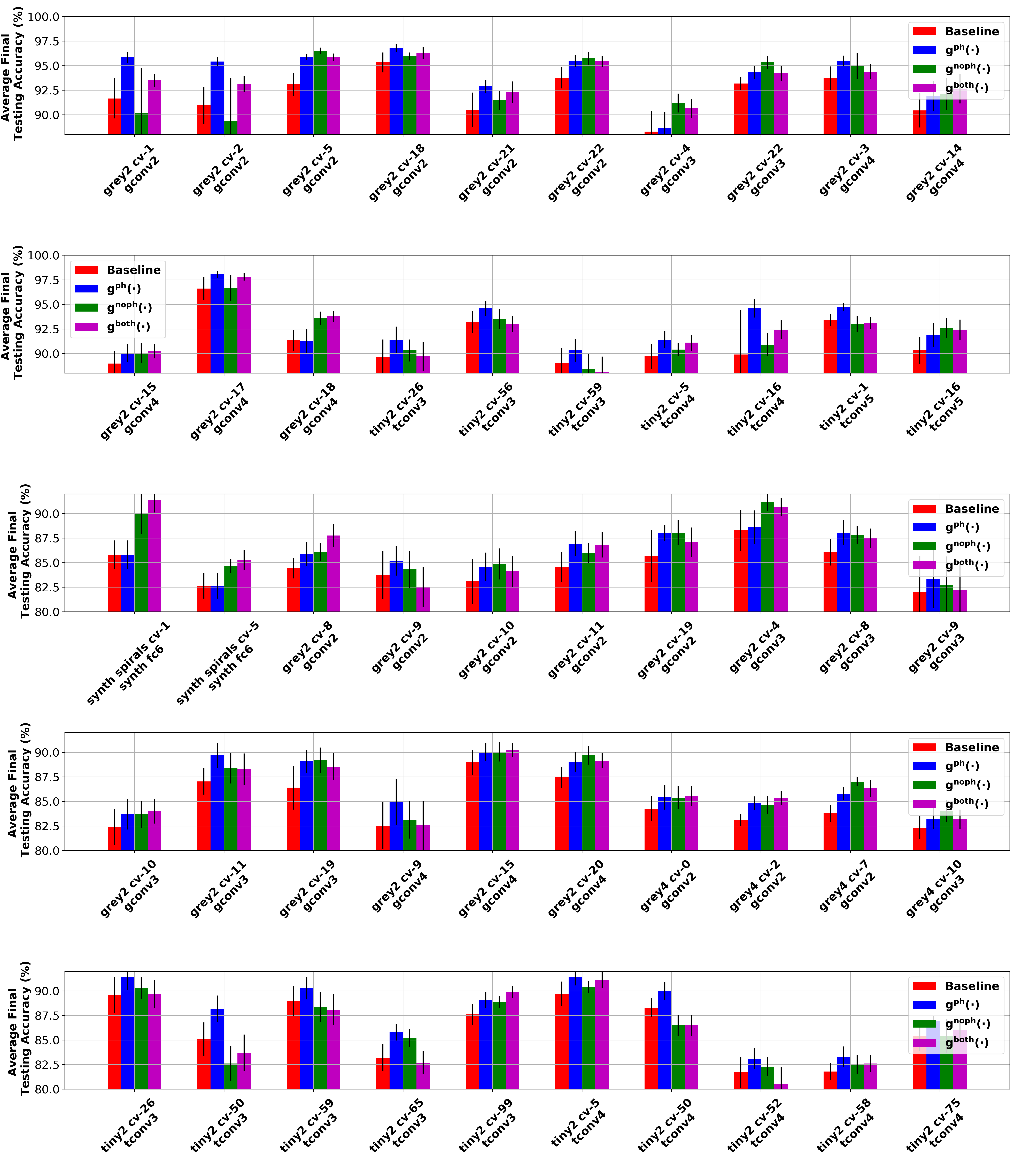
Figure 5: Shown above is the average final testing performance recorded after training (10 initialization for each model and task standard error denoted in black). We show there are classification problems where the topological meta-learning strategies consistently outperform the baseline training procedure denoted in red

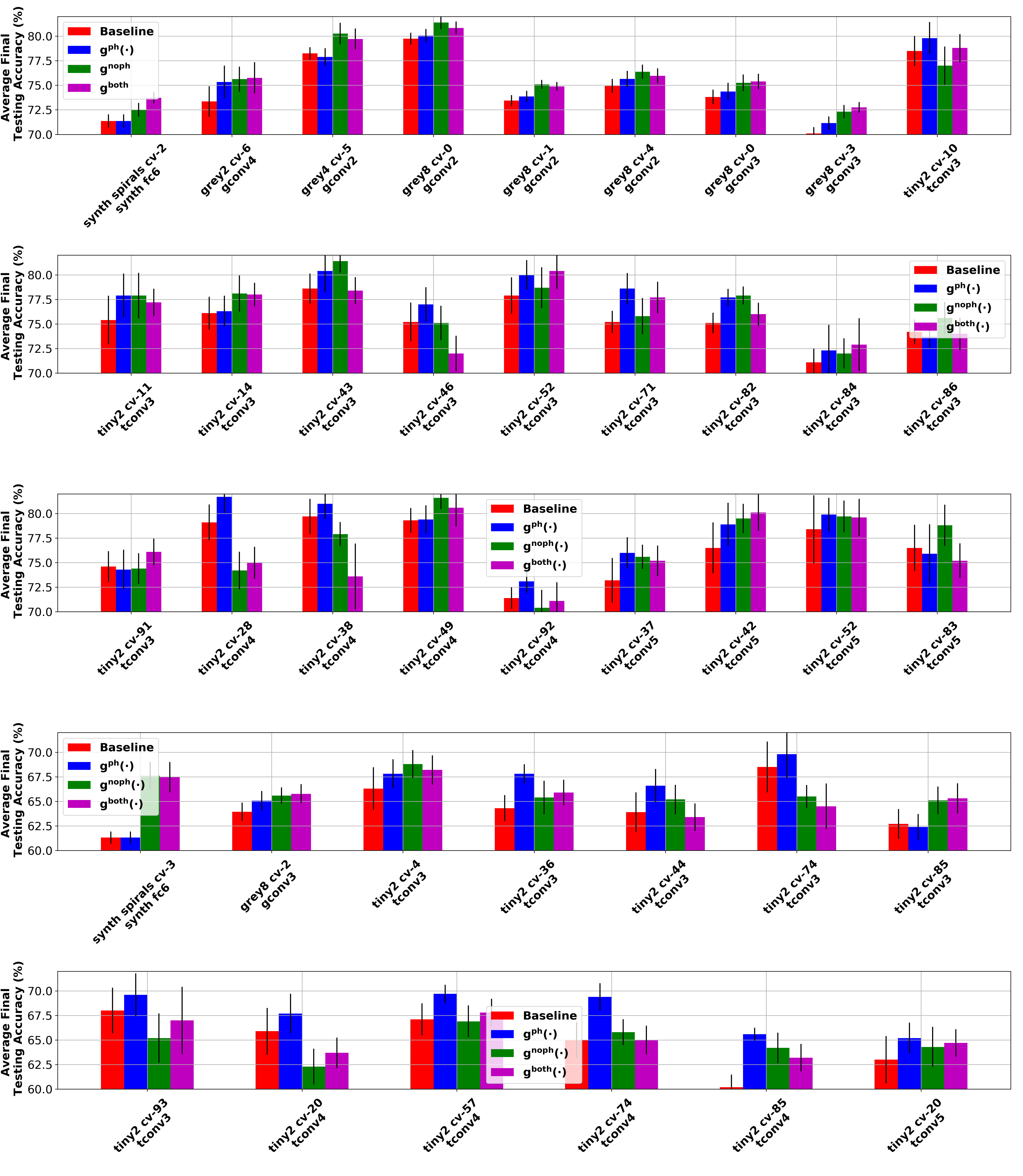
Figure 6: Additional results depict the effects of our meta-learning strategy on more challenging tasks. We similarly show there are classification problems where the topological meta-learning strategies consistently outperform the baseline training procedure denoted in red.

Fine-tuning Pre-trained Models for Task-Similarity: When fine-tuning models we apply the same training procedure as the models trained on the smaller training sets. The only distinction is that models were initialized using the parameters saved after the conventional training procedure from a different classification task. Recall we only select pre-trained parameters from models trained on tasks that differ from the current task being fine-tuned. To keep our model bank $\mathbfcal{F}_{s}$ small during cross-validation, we only consider one model initialization from each class. However, we fine-tune each model with 10 different small training sets. For the Tiny 2 Dataset, we select a subset of models to ensure the number of models needed for fine-tuning was attainable. See supplementary material for additional details.

Topological Feature Generation For Performance Evaluation, Task-Similarity, and Meta-Learning: To generate the topological features from each model for the performance estimation and meta-learning strategy, we pass the entire training set into the model. We then record the training and testing accuracy. We do this first before and after each training procedure. Additional details regarding our particular selection of nodes are defined in equations 16,17 and 23 is located in our supplementary material. All lasso models $h$,$h^{\prime}$, and $h^{\prime\prime}$ are equipped with an alpha term of .01 and k=3 for each k-nearest neighbor models to infer model state.

Training Models with Topological Constraints and Performance Evaluation: We use the same parameter initialization and sub-sampled training data as the DNNs that were prone to overfit. However, we train using our meta-learning strategy as defined in Section 5.3. We construct $\mathbf{T^{*}}$ by selecting topological features induced by DNNs of the same architecture conventionally trained on other classification tasks where testing performance indicates that the models were properly trained, i.e., the gap between training and testing accuracy is small and the testing accuracy is above a particular threshold.

Models are evaluated after each training step. Models are evaluated using the same sequestered testing dataset until training accuracy remains constant. This usually occurs between 100 to 250 steps. For comparison, we compared the final recorded testing accuracy throughout training for the case with and without the topological regularizer. Figures 5 and 6 shows examples of some of the partitions of the data for synthetic, greyscale, and tiny-ImageNet datasets. Additional details about the meta-learning procedure are found in the supplementary material.

7 Results

Performance Estimation Results: We evaluate our performance estimation via $|C|$-fold cross-validation where $|C|$ denotes the number of classification tasks in each parent class. For the intended model state estimation we compute the average classification accuracy across tasks for our nearest neighbor models $\mathbb{N}\mathbb{N}_{k}$. The performance of the linear models $h$ and $h^{\prime}$ used to estimate the testing performance and performance gap are evaluated using the mean absolute error between estimated values and true values. Table II exhibits our ability to estimate the performance of a given model. We can relatively easily infer between model states even with features that do not require persistent homology analysis. Our testing accuracy prediction is under 10.0% overall in terms of mean absolute error. We observed a similar trend in performance gap estimation. and find that out performance gap estimation is under 7.0% in terms of mean absolute error.

Task-Similarity To evaluate task similarity we consider how well $h^{\prime\prime}$ was in selecting the most appropriate model for fine-tuning. We accomplish this by ranking our model selection with respect to all of the other models that could have been selected according to their fine-tuning performance on the current tasks. Additionally, we compute the correlation between the estimated fine-tuning performance from $h^{\prime\prime}$ with the actual fine-tuning performance for each task. Lastly, we compare the selected fine-tuning accuracy in comparison to the average fine-tuning accuracy of the DNNs being fine-tuned. Similar to the previously defined performance estimation strategy, we applied this method in a leave one task out cross-validation procedure, meaning that we trained models using models trained on every task but task $\mathcal{T}_{c}$. Results are shown and described in Table III. We can see this simple linear model is effective in selecting appropriate models as we consistently achieve a better testing performance than the expected testing performance of a randomly selected model for fine-tuning.

Meta-Learning: We examine how our topological meta-learning strategy impacts the testing performance of models being trained on smaller training sets. As previously defined in the main manuscript we quantify performance by examining the final recorded testing accuracy after training. In Figures 5 and 6 we show a set of sample classification problems where our meta-learning optimization strategy improves testing performance. Baseline training is denoted in red while the other colors refer to various topological characterizations with the same hyperparameter selection. Error bars are a result of multiple trials using different initializations and training data samples. We find that there are many classification problems that benefit consistently from our meta-learning strategy. Moreover, this strategy appears to be consistently successful across various architectures tackling the same task.

8 Discussion & Conclusion

We consider further avenues of exploration for the topological analysis of deep networks. One possible avenue is to more deeply understand the meaning of each of these topological features that are useful for performance estimation. One interpretation of previous works which use persistent homology of deep networks is that it can be used to quantify the sparsity of the computational graph in the DNN. This is consistent with previous works like “the lottery ticket hypothesis” [32] which claims there exists a sub-graph within DNNs that is doing the majority of the computational work. Though our characterization was inspired by previous topological characterizations, the interpretation of model sparsity is not so explicit. Examining how our features correlate with previous topological characterizations may be of interest. Additionally, we hope this work inspires others to characterize the structure of DNNs while being less computationally expensive.

Another avenue would be to construct topological characterizations which are invariant to architecture. Since many of our topological features consider local structures of the DNN, it would be possible to compare components of a given network with another component of a network, even if both models consist of different architectures. Lastly, topological characterizations for novel architectures like transformers should be explored.

In summary, we proposed a practical framework to topologically characterize fully connected and convolutional layers in DNNs. Our proposed topological features are quick to compute, differentiable, and can be used in a variety of applications. We showed that the topological characterization can be used to estimate the progress of learning. We also showed its use in examining whether a model was appropriate for fine-tuning on a new task. In addition, we proposed a meta-learning strategy that forces DNNs to elicit topological features consistent with learning. We show that this topological regularization can improve testing performance across numerous datasets and architectures.

Stuart Synakowski received bachelors degrees in Physics and Applied Mathematics/Statistics at Clarkson University, Potsdam, New York in 2017. During his undergraduate studies, he partook in computational biophysics research. He is currently a Ph.D. candidate in Electrical and Computer Engineering at The Ohio State University, working as a research assistant within the Computational Biology and Cognitive Science Lab. His current research interests are in topological data analysis (TDA) applied to improving the performance and understanding of deep neural networks. He is also interested in developing computer vision systems equipped with higher-level action understanding of agents.

Fabian Benitez-Quiroz received the BS degree in electrical engineer- ing from Pontificia Universidad Javeriana, Cali, Colombia, in 2004, the MS degree in electrical engineering from the University of Puerto Rico, Mayaguez, Puerto Rico, in 2008, and the PhD degree in electrical and computer engineering from the Ohio State University (OSU), in 2015. He is currently a postdoctoral researcher with the Computational Biology and Cognitive Science Lab at OSU. His current research interests include the analysis of facial expressions in the wild, functional data analysis, deformable shape detection, face perception, and deep learning . He is a member of the IEEE.

Aleix M. Martinez Aleix M. Martinez is a professor with the Depart- ment of Electrical and Computer Engineering, The Ohio State University (OSU), where he is the founder and director of the Computational Biology and Cognitive Science Lab. He is also affiliated with the Department of Biomedical Engi- neering and to the Center for Cognitive and Brain Sciences, where he is a member of the executive committee. He has served as an associate editor of the IEEE Transactions on Pattern Analysis and Machine Intelligence, the IEEE Transactions on Affective Computing, Image and Vision Computing, and Computer Vision and Image Understanding. He has been an area chair for many top conferences and was program chair for CVPR, 2014. He is also a member of NIH’s Cognition and Perception study section. He is most known for being the first to define many problems and solutions in face recognition (e.g., recognition under occlusions, expression, imprecise landmark detection), discriminant analysis (e.g., Bayes optimal solu- tions, subclass-approaches, optimal kernels), structure from motion (e.g., using kernel mappings to better model non-rigid deformations, noise invariance), and, most recently, demonstrating the existence of a much larger set of cross-cultural facial expressions of emotion than previously known (i.e., compound expressions of emotion) and the transmission of emotion through changes in facial color

References

- [1] J. Deng, W. Dong, R. Socher, L.-J. Li, K. Li, and L. Fei-Fei, “Imagenet: A large-scale hierarchical image database,” in 2009 IEEE conference on computer vision and pattern recognition. Ieee, 2009, pp. 248–255.
- [2] M. Belkin, D. Hsu, S. Ma, and S. Mandal, “Reconciling modern machine-learning practice and the classical bias–variance trade-off,” Proceedings of the National Academy of Sciences, vol. 116, no. 32, pp. 15 849–15 854, 2019.
- [3] T. J. Sejnowski, “The unreasonable effectiveness of deep learning in artificial intelligence,” Proceedings of the National Academy of Sciences, vol. 117, no. 48, pp. 30 033–30 038, 2020.
- [4] P. Y. Lum, G. Singh, A. Lehman, T. Ishkanov, M. Vejdemo-Johansson, M. Alagappan, J. Carlsson, and G. Carlsson, “Extracting insights from the shape of complex data using topology,” Scientific reports, vol. 3, no. 1, pp. 1–8, 2013.
- [5] C. A. Corneanu, M. Madadi, S. Escalera, and A. M. Martinez, “What does it mean to learn in deep networks? and, how does one detect adversarial attacks?” in Proceedings of the IEEE Conference on Computer Vision and Pattern Recognition, 2019, pp. 4757–4766.
- [6] B. Rieck, M. Togninalli, C. Bock, M. Moor, M. Horn, T. Gumbsch, and K. Borgwardt, “Neural persistence: A complexity measure for deep neural networks using algebraic topology,” arXiv preprint arXiv:1812.09764, 2018.
- [7] R. B. Gabrielsson and G. Carlsson, “Exposition and interpretation of the topology of neural networks,” 2019.
- [8] C. A. Corneanu, M. Madadi, S. Escalera, and A. M. Martinez, “Computing the testing error without a testing set,” in Proceedings of the IEEE Conference on Computer Vision and Pattern Recognition, 2020.
- [9] G. Carlsson and R. B. Gabrielsson, “Topological approaches to deep learning,” arXiv preprint arXiv:1811.01122, 2018.
- [10] T. Gebhart, P. Schrater, and A. Hylton, “Characterizing the shape of activation space in deep neural networks,” in 2019 18th IEEE International Conference On Machine Learning And Applications (ICMLA). IEEE, 2019, pp. 1537–1542.
- [11] T. Gebhart and P. Schrater, “Adversary detection in neural networks via persistent homology,” arXiv preprint arXiv:1711.10056, 2017.
- [12] D. Pérez-Fernández, A. Gutiérrez-Fandiño, J. Armengol-Estapé, and M. Villegas, “Characterizing and measuring the similarity of neural networks with persistent homology,” 2021.
- [13] W. H. Guss and R. Salakhutdinov, “On characterizing the capacity of neural networks using algebraic topology,” arXiv preprint arXiv:1802.04443, 2018.
- [14] S. Watanabe and H. Yamana, “Deep neural network pruning using persistent homology,” in 2020 IEEE Third International Conference on Artificial Intelligence and Knowledge Engineering (AIKE), 2020, pp. 153–156.
- [15] M. G. Bergomi, P. Frosini, D. Giorgi, and N. Quercioli, “Towards a topological–geometrical theory of group equivariant non-expansive operators for data analysis and machine learning,” Nature Machine Intelligence, vol. 1, no. 9, pp. 423–433, 2019.
- [16] X. Hu, F. Li, D. Samaras, and C. Chen, “Topology-preserving deep image segmentation,” in Advances in Neural Information Processing Systems, 2019, pp. 5658–5669.
- [17] M. Haft-Javaherian, M. Villiger, C. B. Schaffer, N. Nishimura, P. Golland, and B. E. Bouma, “A topological encoding convolutional neural network for segmentation of 3d multiphoton images of brain vasculature using persistent homology,” in Proceedings of the IEEE/CVF Conference on Computer Vision and Pattern Recognition Workshops, 2020, pp. 990–991.
- [18] J. Clough, N. Byrne, I. Oksuz, V. A. Zimmer, J. A. Schnabel, and A. King, “A topological loss function for deep-learning based image segmentation using persistent homology,” IEEE Transactions on Pattern Analysis and Machine Intelligence, pp. 1–1, 2020.
- [19] M. Moor, M. Horn, B. Rieck, and K. Borgwardt, “Topological autoencoders,” arXiv preprint arXiv:1906.00722, 2019.
- [20] C. Chen, X. Ni, Q. Bai, and Y. Wang, “A topological regularizer for classifiers via persistent homology,” arXiv preprint arXiv:1806.10714, 2018.
- [21] R. Brüel-Gabrielsson, B. J. Nelson, A. Dwaraknath, P. Skraba, L. J. Guibas, and G. Carlsson, “A topology layer for machine learning,” arXiv preprint arXiv:1905.12200, 2019.
- [22] H. Edelsbrunner and J. Harer, Computational topology: an introduction. American Mathematical Soc., 2010.
- [23] M. Carrière, F. Chazal, Y. Ike, T. Lacombe, M. Royer, and Y. Umeda, “Perslay: A neural network layer for persistence diagrams and new graph topological signatures,” in International Conference on Artificial Intelligence and Statistics. PMLR, 2020, pp. 2786–2796.
- [24] C. S. Pun, K. Xia, and S. X. Lee, “Persistent-homology-based machine learning and its applications–a survey,” arXiv preprint arXiv:1811.00252, 2018.
- [25] P. Bubenik et al., “Statistical topological data analysis using persistence landscapes.” J. Mach. Learn. Res., vol. 16, no. 1, pp. 77–102, 2015.
- [26] M. Gabella, N. Afambo, S. Ebli, and G. Spreemann, “Topology of learning in artificial neural networks,” arXiv preprint arXiv:1902.08160, 2019.
- [27] F. Pedregosa, G. Varoquaux, A. Gramfort, V. Michel, B. Thirion, O. Grisel, M. Blondel, P. Prettenhofer, R. Weiss, V. Dubourg, J. Vanderplas, A. Passos, D. Cournapeau, M. Brucher, M. Perrot, and E. Duchesnay, “Scikit-learn: Machine learning in Python,” Journal of Machine Learning Research, vol. 12, pp. 2825–2830, 2011.
- [28] Y. LeCun and C. Cortes, “MNIST handwritten digit database,” 2010. [Online]. Available: http://yann.lecun.com/exdb/mnist/
- [29] T. Clanuwat, M. Bober-Irizar, A. Kitamoto, A. Lamb, K. Yamamoto, and D. Ha, “Deep learning for classical japanese literature,” arXiv preprint arXiv:1812.01718, 2018.
- [30] G. Cohen, S. Afshar, J. Tapson, and A. Van Schaik, “Emnist: Extending mnist to handwritten letters,” in 2017 International Joint Conference on Neural Networks (IJCNN). IEEE, 2017, pp. 2921–2926.
- [31] J. Wu, Q. Zhang, and G. Xu, “Tiny imagenet challenge,” Tech. Rep.
- [32] J. Frankle and M. Carbin, “The lottery ticket hypothesis: Finding sparse, trainable neural networks,” arXiv preprint arXiv:1803.03635, 2018.