The Quantum Multiple-Access Channel with Cribbing Encoders

Abstract

Communication over a quantum multiple-access channel (MAC) with cribbing encoders is considered, whereby Transmitter 2 performs a measurement on a system that is entangled with Transmitter 1. Based on the no-cloning theorem, perfect cribbing is impossible. This leads to the introduction of a MAC model with noisy cribbing. In the causal and non-causal cribbing scenarios, Transmitter 2 performs the measurement before the input of Transmitter 1 is sent through the channel. Hence, Transmitter 2’s cribbing may inflict a “state collapse” for Transmitter 1. Achievable regions are derived for each setting. Furthermore, a regularized capacity characterization is established for robust cribbing, i.e. when the cribbing system contains all the information of the channel input. Building on the analogy between the noisy cribbing model and the relay channel, a partial decode-forward region is derived for a quantum MAC with non-robust cribbing. For the classical-quantum MAC with cribbing encoders, the capacity region is determined with perfect cribbing of the classical input, and a cutset region is derived for noisy cribbing. In the special case of a classical-quantum MAC with a deterministic cribbing channel, the inner and outer bounds coincide.

I Introduction

The multiple-access channel (MAC) is among the most fundamental and well-understood models in network communication and information theory [1, 2]. The MAC is also referred to as the uplink channel [3], since it is interpreted in cellular communication as the link from the mobiles to the base station [4], and in the satellite-based Internet of Things (IoT), from ground devices to a satellite in space [5]. Furthermore, in a wireless local area network (WLAN), the MAC represents the channel from the terminals to the access point [6, Section 3.2]. In general, the signals of different transmitters may interfere with one another. In particular, in sequential decoding, the receiver first decodes the message of one of the transmitters, while treating the other signals as noise. Then, this estimation can be used in order to reduce the effective noise for the estimation of the next message. Following this interplay, if a cognitive transmitter has access to the signal of another transmitter, this knowledge can be exploited such that the receiver will decode the messages with less noise. Such scenarios naturally arise in wireless systems of cognitive radios [7, 8] and the Internet of Things (IoT) [9]. This motivates the study of the MAC with cribbing encoders, i.e. the channel setting where one transmitter has access to the signal of another transmitter [10].

Cooperation in quantum communication networks has been extensively studied in recent years, following both experimental progress and theoretical discoveries [11, 12]. Quantum MACs are considered in the literature in various settings. Winter [13] derived a regularized characterization for the classical capacity region of the quantum MAC (see also [14]). Hsieh et al. [15] and Shi et al. [16] addressed the model where each transmitter shares entanglement resources with the receiver independently. Furthermore, Boche and Nötzel [17] addressed the cooperation setting of a classical-quantum MAC with conferencing encoders, where the encoders exchange messages between them in a constant rate (see also [18]). Remarkably, Leditzky et al. [19] have shown that sharing entanglement between transmitters can strictly increase the achievable rates for a classical MAC. The channel construction in [19] is based on a pseudo-telepathy game [20] where quantum strategies guarantee a certain win and outperform classical strategies. The authors of the present paper [21] have recently shown that the dual property does not hold, i.e. entanglement between receivers does not increase achievable rates. Related settings of the quantum MAC involve transmission of quantum information [22, 23], error exponents [24], non-additivity effects [25], security [26, 27, 28, 29], and computation codes [30].

The sixth generation of cellular networks (6G) is expected to achieve gains in terms of latency, resilience, computation power, and trustworthiness in future communication systems, such as the tactile internet [31], which not only transfer data but also control physical and virtual objects, by using quantum resources [32]. Cooperation between trusted hardware and software components in future communication systems has the potential to isolate untrusted components such that the attack surface of the communication system is substantially reduced [31, 33]. Quantum resources and cooperation offer additional advantages, in terms of performance gains for communication tasks and reduction of attack surface, and are of great potential for 6G networks [34, 35]. It is therefore interesting to investigate cooperation for quantum MACs as a technique to achieve robust efficient protocols for future applications.

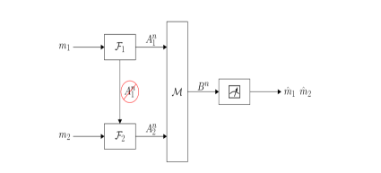
Figure 1: The quantum multiple-access channel $\mathcal{M}_{A_{1}A_{2}\rightarrow B}$ with cribbing at Encoder 2.

(a) Perfect cribbing violates the laws of quantum mechanics. If Encoder 1 sends $A_{1}$ through the channel, then Encoder 2 is physically prohibited from having a copy of the input state.

(b) A quantum MAC $\mathcal{N}\circ\mathcal{L}$ with noisy cribbing. Alice 1 sends the input system $A_{1}^{n}$ through $n$ copies of a cribbing channel $\mathcal{L}_{A_{1}\to A_{1}^{\prime}E}$, producing two outputs, $A_{1}^{\prime n}$ and $E^{n}$. Alice 2 performs a measurement on the system $E^{n}$, and uses the measurement outcome in order to encode the input state of $A_{2}^{n}$. Then, the input systems $A_{1}^{\prime n}$ and $A_{2}^{n}$ are sent through $n$ copies of the communication channel $\mathcal{N}_{A_{1}^{\prime}A_{2}\to B}$. The model can also be interpreted as if the second transmitter performs a measurement on the environment $E^{n}$ of the first transmitter.

The classical MAC with cribbing encoders is a channel model with two transmitters, $X_{1}$ and $X_{2}$, and a single receiver, $Y$, where one transmitter has access to the other’s transmissions. Willems and van der Meulen [36] introduced this setting and considered different scenarios of full cribbing, i.e. with a perfect copy of the other sender’s input. Suppose that Transmitter 2 knows $X_{1}$. Asnani and Permuter [37] pointed out that for a Gaussian channel, the full cribbing model is degenerate, as it reduces to full cooperation since a noiseless transmission of a continuous signal $X_{1}$ allows sending an infinite amount of information from Transmitter 1 to Transmitter 2. This has motivated Asnani and Permuter to consider the MAC with partial cribbing, with a “discretized” version of the other input. Specifically, Transmitter 2 may have access to $Z=g(X_{1})$, instead of $X_{1}$, where $g(\cdot)$ is a deterministic function. See [37, 38] for further details. The original work of Willems and van der Meulen [36] included different causality scenarios, where the sender(s) have the $i$th copy of each other’s inputs, either after sending their own transmission at time $i$ (strictly-causal cribbing), before the $i$th transmission (causal cribbing), or a priori before transmission takes place (non-causal cribbing). Classical cribbing is further studied in [39, 40, 41, 42, 43, 44, 45, 46, 47].

The MAC with cribbing encoders is closely-related to the relay channel [48, 49]. Even in the classical case, the capacity of the relay channel is an open problem. Savov et al. [50, 14] derived a partial decode-forward lower bound for the classical-quantum relay channel, where the relay encodes information in a strictly-causal manner. Recently, Ding et al. [51] generalized those results and established the cutset, multihop, and coherent multihop bounds. Communication with the help of environment measurement can be modeled by a quantum channel with a classical relay in the environment [52]. Considering this setting, Smolin et al. [53] and Winter [54] determined the environment-assisted quantum capacity and classical capacity, respectively. Savov et al. [50] further discussed future research directions of interest, and pointed out that quantum communication scenarios over the relay channel may have applications for the design of quantum repeaters [50, Section V.] (see also [51]). In a recent work by the authors [21], we have considered the quantum broadcast channel with conferencing receivers, and provided an information-theoretic perspective on quantum repeaters through this setting.

In this paper, we consider the quantum MAC $\mathcal{M}_{A_{1}A_{2}\to B}$ with cribbing encoders. In quantum communication, the description is more delicate. By the no-cloning theorem, universal copying of quantum states is impossible. Therefore, in the view of quantum mechanics, perfect cribbing is against the laws of nature. As illustrated in Figure 1, if Encoder 1 sends $A_{1}$ through the channel, then Encoder 2 is physically prohibited from having a copy of the input state. Hence, we consider the quantum MAC with noisy cribbing, consisting of a concatenation of a cribbing channel and the communication channel (see Figure 1b). Specifically, Encoder 1 sends the input system $A_{1}$ through a cribbing channel that has two outputs, $A_{1}^{\prime}$ and $E$. Encoder 2 performs a measurement on the system $E$, and uses the measurement outcome in order to encode the input state of $A_{2}$. Then, the input systems $A_{1}^{\prime}$ and $A_{2}$ are sent through the communication channel. The model can also be interpreted as if the second transmitter performs a measurement on the environment $E$ of the first transmitter.

The entanglement between the cribbing system $E$ and the communication channel input $A_{1}^{\prime}$ has the following implication. If Encoder 2 measures $E_{i}$ before $A_{1,i}^{\prime}$ is sent through the channel, as in the causal and non-causal scenarios, then Encoder 2’s cribbing measurement may inflict a “state collapse” of Encoder 1’s transmission through the communication channel. In other words, in quantum communication, the cribbing operation interferes with Encoder 1’s input before it is even transmitted through the communication channel.

We consider the scenarios of strictly-causal, causal, and non-causal cribbing. For a MAC with robust cribbing, the cribbing system $E$ includes all the information that is available in $A_{1}^{\prime}$. We derive achievable regions for each setting and establish a regularized capacity characterization for robust cribbing. Building on the analogy between the noisy cribbing model and the relay channel, we further develop a partial decode-forward region for the quantum MAC with strictly-causal non-robust cribbing. For the classical-quantum MAC with cribbing encoders, the capacity region is determined with perfect cribbing of the classical input, and a cutset region is derived for noisy cribbing. In the special case of a classical-quantum MAC with a deterministic cribbing channel, the inner and outer bounds coincide. The setting of noisy cribbing is significantly more challenging, as it is closely-related to the relay channel. The comparison between the relay channel and the MAC with cribbing encoders is further investigated in the present paper. We derive a generalized packing lemma for the MAC. While the lemma does not include cribbing, it is useful in the analysis of the MAC with cribbing encoders.

The paper is organized as follows. In Section II, we give the definitions of the channel model and a brief review of related work. In Section III, we provide the information-theoretic tools for the analysis and state the generalized quantum packing lemma. The main results are given in Section IV and Section V. In the former, we focus on robust cribbing, and in the latter, we introduce partial decode-forward coding for the non-robust case. The proofs are given in the appendix.

II Definitions and Related Work

II-A Notation, States, and Information Measures

We use the following notation conventions. Script letters $\mathcal{X},\mathcal{Y},\mathcal{Z},...$ are used for finite sets. Lowercase letters $x,y,z,\ldots$ represent constants and values of classical random variables, and uppercase letters $X,Y,Z,\ldots$ represent classical random variables. The distribution of a random variable $X$ is specified by a probability mass function (pmf) $p_{X}(x)$ over a finite set $\mathcal{X}$. We use $x^{j}=(x_{1},x_{2},\ldots,x_{j})$ to denote a sequence of letters from $\mathcal{X}$. A random sequence $X^{n}$ and its distribution $p_{X^{n}}(x^{n})$ are defined accordingly.

The state of a quantum system $A$ is a density operator $\rho$ on the Hilbert space $\mathcal{H}_{A}$. A density operator is an Hermitian, positive semidefinite operator, with unit trace, i.e. $\rho^{\dagger}=\rho$, $\rho\succeq 0$, and $\mathrm{Tr}(\rho)=1$. The set of all density operators acting on $\mathcal{H}_{A}$ is denoted by $\mathscr{D}(\mathcal{H}_{A})$. The state is said to be pure if $\rho=|\psi\rangle\langle\psi|$, for some vector $|\psi\rangle\in\mathcal{H}_{A}$. Define the quantum entropy of the density operator $\rho$ as $H(\rho)\triangleq-\mathrm{Tr}[\rho\log(\rho)]$. Consider the state of a pair of systems $A$ and $B$ on the product space $\mathcal{H}_{A}\otimes\mathcal{H}_{B}$. Given a bipartite state $\sigma_{AB}$, define the quantum mutual information as

$$I(A;B)_{\sigma}=H(\sigma_{A})+H(\sigma_{B})-H(\sigma_{AB})\,.$$ (1)

Furthermore, conditional quantum entropy and mutual information are defined by $H(A|B)_{\sigma}=H(\sigma_{AB})-H(\sigma_{B})$ and $I(A;B|C)_{\sigma}=H(A|C)_{\sigma}+H(B|C)_{\sigma}-H(AB|C)_{\sigma}$, respectively. A quantum channel $\mathcal{P}_{A\to B}$ is a completely-positive trace-preserving (cptp) linear map from $\mathscr{D}(\mathcal{H}_{A})$ to $\mathscr{D}(\mathcal{H}_{B})$.

A measurement of a quantum system is specified in two equivalent manners. When the post-measurement state is irrelevant, we specify a measurement by a positive operator-valued measure (POVM), i.e. a set of positive semi-denfinite operators $\{K_{x}\}_{x\in\mathcal{X}}$ such that $\sum_{x}K_{x}=\text{1}$. According to the Born rule, if the system is in state $\rho$, then the probability to measure $x$ is $p_{X}(x)=\mathrm{Tr}(K_{x}\rho)$. More generally, a measurement is defined by a set of operators $\{W_{x}\}_{x\in\mathcal{X}}$ such that $\sum_{x}W_{x}^{\dagger}W_{x}=\text{1}$. If the system is in the state $\rho$, then the measurement outcome $X$ is distributed by $p_{X}(x)=\mathrm{Tr}(W_{x}^{\dagger}W_{x}\rho)$ for $x\in\mathcal{X}$. If $X=x$ was measured, then the post-measurement state is $\rho^{\prime}\equiv(W_{x}\rho W_{x}^{\dagger})/\mathrm{Tr}(W_{x}^{\dagger}W_{x}\rho)$. Furthermore, the quantum instrument $\mathcal{W}_{A\to\bar{A}X}$ of this measurement is the linear map from the original state, before the measurement, to the joint state of the system after the measurement with the measurement outcome, i.e.

$$\mathcal{W}_{A\to\bar{A}X}(\rho)=\sum_{x\in\mathcal{X}}W_{x}\rho W_{x}^{\dagger}\otimes|x\rangle\langle x|\,.$$ (2)

A quantum Markov chain is defined as follows. The quantum systems $A\leavevmode\hbox to9.01pt{\vbox to4.71pt{\text{[drawing]}}}B\leavevmode\hbox to9.01pt{\vbox to4.71pt{\text{[drawing]}}}C$ form a Markov chain if there exists a recovery channel $\mathcal{P}_{B\rightarrow BC}$ such that $\rho_{ABC}=(\mathrm{id}_{A}\otimes\mathcal{P}_{B\rightarrow BC})(\rho_{AB})$ [55]. In general, this holds if and only if

$$I(A;C|B)_{\rho}=0$$ (3)

(see [55, Theorem 5.2]).

II-B Quantum Multiple-Access Channel

A quantum multiple-access channel (MAC) maps a quantum state at the senders’ system to a quantum state at the receiver. Here, we consider a channel with two transmitters. Formally, a quantum MAC is a cptp map $\mathcal{M}_{A_{1}A_{2}\rightarrow B}$ corresponding to a quantum physical evolution. We assume that the channel is memoryless. That is, if the systems $A_{1}^{n}=(A_{1,i})_{i=1}^{n}$ and $A_{2}^{n}=(A_{2,i})_{i=1}^{n}$ are sent through $n$ channel uses, then the joint input state $\rho_{A_{1}^{n}A_{2}^{n}}$ undergoes the tensor product mapping $\mathcal{M}_{A_{1}^{n}A_{2}^{n}\rightarrow B^{n}}\equiv\mathcal{M}_{A_{1}A_{2}\rightarrow B}^{\otimes n}$.

We will consider a MAC with cribbing, where Transmitter 2 can measure a system $E$ that is entangled with Transmitter 1’s system. Assume without loss of generality that the quantum MAC can be decomposed as

$$\mathcal{M}_{A_{1}A_{2}\to B}(\rho_{A_{1}A_{2}})=\mathrm{Tr}_{E}\left[(\mathcal{N}_{A_{1}^{\prime}A_{2}\to B}\circ\mathcal{L}_{A_{1}\to A_{1}^{\prime}E})(\rho_{A_{1}A_{2}})\right]$$ (4)

for all $\rho_{A_{1}A_{2}}$, and some channel $\mathcal{L}_{A_{1}\to A_{1}^{\prime}E}$. In general, there always exists such a channel, since we can define $\mathcal{L}_{A_{1}\to A_{1}^{\prime}E}$ such that the outputs $A_{1}^{\prime}$ and $E$ are in a product state and $\rho_{A_{1}^{\prime}}=\rho_{A_{1}}$. However, the interesting case is when the transmitted system $A_{1}^{\prime}$ and the cribbing system $E$ are correlated.

The transmitters and the receiver are often called Alice 1, Alice 2, and Bob. In the cribbing setting, Alice 1 first sends the input state of $A_{1}^{n}$ through the channel $\mathcal{L}_{A_{1}^{n}\to A_{1}^{\prime n}E^{n}}\equiv\mathcal{L}^{\otimes n}_{A_{1}\to A_{1}^{\prime}E}$. Alice 2 gains access to the system $E^{n}$, and performs a measurement. Then, she encodes the state of her input $A_{2}^{n}$ using the measurement outcome, and transmits it to Bob. Henceforth, we will refer to the channel $\mathcal{L}_{A_{1}\to A_{1}^{\prime}E}$ as the cribbing channel, and to $E^{n}$ as the cribbing system. We denote the quantum MAC with cribbing by $\mathcal{N}_{A_{1}^{\prime}A_{2}\to B}\circ\mathcal{L}_{A_{1}\to A_{1}^{\prime}E}$.

In the sequel, we will also be interested in the following special cases.

Definition 1.

Let $\mathcal{N}\circ\mathcal{L}$ be a quantum MAC with cribbing. Given an input state $\theta_{A_{1}A_{0}}$, where $A_{0}$ is an arbitrary reference system, let $\rho_{A_{1}^{\prime}EA_{0}}=\mathcal{L}_{A_{1}\to A_{1}^{\prime}E}(\theta_{A_{1}A_{0}})$ be the output of the cribbing channel. We say that the quantum MAC is with robust cribbing if $A_{0}\leavevmode\hbox to9.01pt{\vbox to4.71pt{\text{[drawing]}}}E\leavevmode\hbox to9.01pt{\vbox to4.71pt{\text{[drawing]}}}A_{1}^{\prime}$ form a quantum Markov chain.

That is, for every input $\theta_{A_{1}A_{0}}$, there exists a recovery channel $\mathcal{P}^{\theta}_{E\to A_{1}^{\prime}E}$ such that

$$\rho_{A_{1}^{\prime}EA_{0}}=\mathcal{P}^{\theta}_{E\to A_{1}^{\prime}E}(\rho_{EA_{0}})\,.$$ (5)

We give the following intuition. In the cribbing setting, Alice 2 may have a noisy copy of Alice 1’s input. The condition above means that Alice 2’s copy is “at least as good” as the one which is transmitted through the channel $\mathcal{N}$. That is, the channel input $A_{1}^{\prime}$ does not contain more information than the cribbing system $E$, which Alice 2 measures. Next, we define the classical-quantum MAC with noiseless cribbing, which is a special case of a quantum MAC with robust cribbing.

Definition 2.

The classical-quantum MAC with noiseless cribbing is defined by $\mathcal{N}\circ\mathcal{L}$ such that the inputs $A_{1}$, $A_{2}$ are classical, and the cribbing channel simply copies Alice 1’s input, i.e. $A_{1}\equiv X_{1}$, $A_{2}\equiv X_{2}$, and $\mathcal{L}=\text{id}_{X_{1}\to X_{1}X_{1}}$. Hence, the cribbing system is an exact copy of Alice 1’s input, i.e.

$$E\equiv A_{1}^{\prime}\equiv A_{1}\equiv X_{1}\,.$$ (6)

We denote the classical-quantum MAC with noiseless cribbing by $\mathcal{N}_{X_{1}X_{2}\to B}\circ\text{id}_{X_{1}\to X_{1}X_{1}}$.

If the cribbing observation is noisy, then it may not satisfy the robustness property.

Definition 3.

The classical-quantum MAC with a noisy cribbing channel $Q_{Z|X_{1}}$ is defined such that the inputs $A_{1}$, $A_{1}^{\prime}$, $A_{2}$ and the cribbing system $E$ are classical, i.e. $A_{1}\equiv A_{1}^{\prime}\equiv X_{1}$, $A_{2}\equiv X_{2}$, and $E\equiv Z$, while the cribbing channel is specified by the classical noisy channel $Q_{Z|X_{1}}$. We denote the classical-quantum MAC with noisy cribbing by $\mathcal{N}_{X_{1}X_{2}\to B}\circ Q_{Z|X_{1}}$.

Remark 1.

Another simple example of robust cribbing is the case where $A_{1}^{\prime}$ does not store information at all, say $|\mathcal{H}_{A_{1}^{\prime}}|=1$. The resulting channel is a basic multi-hop link that concatenates two point-to-point channels. Specifically, Alice 1 sends the input $A_{1}$ to Alice 2 via $\mathcal{L}_{A_{1}\to E}$, Alice 2 measures $E$, encodes the input $A_{2}$, and send it to Bob over $\mathcal{N}_{A_{2}\to B}$.

II-C Coding with Cribbing

We consider different scenarios of cribbing. First, we define the setting of a MAC where Alice 2 obtains her measurements of the systems $E_{1},E_{2},\ldots$ in a causal manner. That is, at time $i$, Alice 2 can measure the past and present systems $E_{1},\ldots,E_{i}$.

Definition 4.

A $(2^{nR_{1}},2^{nR_{2}},n)$ classical code for the quantum MAC $\mathcal{N}_{A_{1}^{\prime}A_{2}\rightarrow B}\circ\mathcal{L}_{A_{1}\to A_{1}^{\prime}E}$ with cribbing consists of the following:

• Two message sets $[1:2^{nR_{1}}]$ and $[1:2^{nR_{2}}]$, assuming $2^{nR_{k}}$ is an integer;

• an encoding map $\mathcal{F}_{1}:[1:2^{nR_{1}}]\to\mathscr{D}(\mathcal{H}_{A_{1}}^{\otimes n})$ for Encoder 1;

• a sequence of cribbing POVMs $\mathcal{K}_{i}=\{K^{z}_{E^{i}}\,,\;z\in\mathcal{Z}\}$, for Encoder 2;

• a sequence of $n$ encoding maps $\mathcal{F}_{2,i}:\mathcal{Z}^{i}\times[1:2^{nR_{2}}]\to\mathscr{D}(\mathcal{H}_{A_{2}}^{\otimes i})$, where $i\in[1:n]$, for Encoder 2; and

• a decoding POVM $\mathcal{D}=\{D^{m_{1},m_{2}}_{B^{n}}\}$, where the measurement outcome is an index pair $(m_{1},m_{2})$, with $m_{k}\in[1:2^{nR_{k}}]$ for $k=1,2$.

The sequence of encoding maps needs to be consistent in the sense that the states $\rho^{m_{2},z^{i}}_{A_{2}^{i}}\equiv\mathcal{F}_{2,i}(z_{1}^{i},m_{2})$ satisfy $\mathrm{Tr}_{A_{2,i+1}^{n}}(\rho^{m_{2},z_{1}^{n}}_{A_{2}^{n}})=\rho^{m_{2},z_{1}^{i}}_{A_{2}^{i}}$. We denote the code by $(\mathcal{F}_{1},\mathcal{F}_{2},\mathcal{K},\mathcal{D})$.

The communication scheme is depicted in Figure 1b. The sender Alice 1 has the input system $A_{1}^{n}$, the sender Alice 2 has both $A_{2}^{n},E^{n}$, and the receiver Bob has $B^{n}$. Alice $k$ chooses a message $m_{k}$ according to a uniform distribution over $[1:2^{nR_{k}}]$, for $k=1,2$. To send the message $m_{1}\in[1:2^{nR_{1}}]$, Alice 1 encodes the message by $\rho_{A_{1}^{n}}^{m_{1}}\equiv\mathcal{F}_{1}(m_{1})$, and sends her transmission $A_{1}^{n}$ through $n$ uses of the cribbing channel. Her transmission induces the following state,

$$\rho^{m_{1}}_{A_{1}^{\prime n}E^{n}}=\mathcal{L}^{\otimes n}(\rho_{A_{1}^{n}}^{m_{1}})$$ (7)

where $E^{n}$ is the cribbing system which will be measured by the second transmitter.

At time $i$, Alice 2 measures the system $E^{i}$ using the measurement $\mathcal{K}_{i}$, and obtains a measurement outcome $z_{i}$. To send the message $m_{2}\in[1:2^{nR_{2}}]$, she prepares the input state $\mathcal{F}_{2,i}(m_{2},z^{i})$ in a causal manner, and sends her transmission. The average joint input state is

$$\rho^{m_{1},m_{2}}_{A_{1}^{\prime n}A_{2}^{n}}=\sum_{z^{n}\in\mathcal{Z}^{n}}\mathrm{Tr}_{E^{n}}\left[(\mathrm{id}\otimes K^{z^{n}})\rho^{m_{1}}_{A_{1}^{\prime n}E^{n}}\right]\otimes\mathcal{F}_{2,n}(m_{2},z^{n})$$ (8)

with $K^{z^{n}}_{E^{n}}\equiv K_{E^{n}}^{z_{n}}K_{E^{n-1}}^{z_{n-1}}\cdots K_{E_{1}}^{z_{1}}$.

Bob receives the channel output systems $B^{n}$ in the following state,

$$\rho^{m_{1},m_{2}}_{B^{n}}=\mathcal{N}^{\otimes n}(\rho^{m_{1},m_{2}}_{A_{1}^{\prime n}A_{2}^{n}})\,.$$ (9)

He measures with the decoding POVM $\mathcal{D}$ and obtains an estimate of the message pair $(\hat{m}_{1},\hat{m}_{2})\in[1:2^{nR_{1}}]\times[1:2^{nR_{2}}]$ from the measurement outcome. The average probability of error of the code is

$$P_{e}^{(n)}(\mathcal{F}_{1},\mathcal{F}_{2},\mathcal{K},\mathcal{D})=\frac{1}{2^{n(R_{1}+R_{2})}}\sum_{m_{1}=1}^{2^{nR_{1}}}\sum_{m_{2}=1}^{2^{nR_{2}}}\left(1-\mathrm{Tr}[D^{m_{1},m_{2}}\rho^{m_{1},m_{2}}_{B^{n}}]\right)\,.$$ (10)

A $(2^{nR_{1}},2^{nR_{2}},n,\varepsilon)$ classical code satisfies $P_{e}^{(n)}(\mathcal{F}_{1},\mathcal{F}_{2},\mathcal{K},\mathcal{D})\leq\varepsilon$. A rate pair $(R_{1},R_{2})$ is called achievable with causal cribbing if for every $\varepsilon>0$ and sufficiently large $n$, there exists a $(2^{nR_{1}},2^{nR_{2}},n,\varepsilon)$ code. The classical capacity region $\mathcal{C}_{\text{caus}}(\mathcal{N}\circ\mathcal{L})$ of the quantum MAC with causal cribbing is defined as the set of achievable pairs $(R_{1},R_{2})$, where the subscript ‘caus’ indicates causal cribbing.

We will also put a considerable focus on strictly-causal and non-causal cribbing. In the strictly-causal setting, Alice 2 can measure the cribbing system only after she has sent her transmission at each time instance. That is, a code with strictly-causal cribbing is defined in a similar manner, where Alice 2 first transmits her input $A_{2,i}$, and only then measures $E^{i}$. Therefore, her input state at time $i$ can only depend on the past measurements $z^{i-1}$, and the $i$th encoding map has the form $\mathcal{F}_{2,i}:\mathcal{Z}^{i-1}\times[1:2^{nR_{2}}]\to\mathscr{D}(\mathcal{H}_{A_{2}}^{\otimes i})$. We denote the capacity region for this scenario by $\mathcal{C}_{\text{s-c}}(\mathcal{N}\circ\mathcal{L})$, where the subscript ’s-c’ stands for strictly-causal cribbing.

With non-causal cribbing, Alice 2 gains access to the entire sequence of systems $E^{n}$ a priori, i.e. before the beginning of her transmission. Thus, she can perform a joint measurement at time $i=1$, with a single POVM $\mathcal{K}=\{K^{\ell}_{E^{n}}\}$, before sending $A_{2}^{n}$. Thereby, she can prepare a joint state $\rho_{A_{2}^{n}}^{m_{2},\ell}$ of any form. The capacity region with non-causal cribbing is denoted by $\mathcal{C}_{\text{n-c}}(\mathcal{N}\circ\mathcal{L})$.

Remark 2.

The MAC with strictly-causal cribbing is closely related to the relay channel. In particular, if we impose $R_{2}=0$, then Alice 2 can only use the cribbing channel to enhance the transmission of information from Alice 1 to Bob. That is, Alice 2 acts as a relay in this case. In the sequel, we will introduce methods for quantum cribbing that are inspired by relay coding techniques. It should be noted, however, that as opposed to the relay channel, our cribbing channel (‘sender-relay link’) is not affected by the transmission of Alice 2 (the ‘relay’). Specifically, Savov et al. [50, 14] considered a relay channel $\mathcal{P}_{A_{1}A_{2}\to EB}$, where the transmitter sends a classical input $A_{1}\equiv X_{1}$, the relay receives $E$ and transmits $A_{2}\equiv X_{2}$, and the destination receiver receives the quantum output $B$. Hence, the state of $E$ in the relay model is affected by both $A_{1}$ and $A_{2}$. Here, on the other hand, the cribbing channel acts only on $A_{1}$. Nonetheless, it appears that the technical challenges carry over from the relay channel to the present model.

Remark 3.

Based on the definitions above, we have the following relation between the capacity regions of the MAC with strictly-causal, causal, and non-causal cribbing: $\mathcal{C}_{\text{s-c}}(\mathcal{N}\circ\mathcal{L})\subseteq\mathcal{C}_{\text{caus}}(\mathcal{N}\circ\mathcal{L})\subseteq\mathcal{C}_{\text{n-c}}(\mathcal{N}\circ\mathcal{L})$. This follows because, if Alice 2 has causal access to $E^{i}$, or to the entire sequence of $E^{n}$, then she can choose to measure only $E^{i-1}$ at time $i$. Hence, every code with strictly-causal cribbing can also be used given causal or non-causal cribbing. Similarly, a causal scheme can be performed given non-causal cribbing.

II-D Related Work

We briefly review the capacity result for the quantum MAC without cribbing. A code without cribbing is defined in a similar manner, where Alice 2 is not allowed to measure the cribbing systems $E^{n}$. In this case, the model is fully described by $\mathcal{M}_{A_{1}A_{2}\to B}$, ignoring its components $\mathcal{L}_{A_{1}\to A_{1}^{\prime}E}$ and $\mathcal{N}_{A_{1}^{\prime}A_{2}\to B}$ (see (4) and Figure 1b). Denote the capacity region without cribbing by $\mathcal{C}_{\text{none}}(\mathcal{M})$. Define a rate region $\mathcal{R}_{\text{none}}(\mathcal{N}\circ\mathcal{L})$ as follows,

$$\mathcal{R}_{\text{none}}(\mathcal{M})=\bigcup_{p_{U}p_{X_{1}|U}p_{X_{2}|U}\,,\;\theta_{A_{1}}^{x_{1}}\otimes\zeta_{A_{2}}^{x_{2}}}\left\{\begin{array}[]{rl}(R_{1},R_{2})\,:\;R_{1}&\leq I(X_{1};B|X_{2}U)_{\omega}\\ R_{2}&\leq I(X_{2};B|X_{1}U)_{\omega}\\ R_{1}+R_{2}&\leq I(X_{1}X_{2};B|U)_{\omega}\end{array}\right\}$$ (14)

where the union is over the joint distributions of the auxiliary random variables $U,X_{1},X_{2}$ and the product state collections $\{\theta_{A_{1}}^{x_{1}}\otimes\zeta_{A_{2}}^{x_{2}}\}$, with

$$\omega_{UX_{1}X_{2}B}=\sum_{u,x_{1},x_{2}}p_{U}(u)p_{X_{1}|U}(x_{1}|u)p_{X_{2}|U}(x_{2}|u)|u\rangle\langle u|$$

$$\otimes|x_{1}\rangle\langle x_{1}|\otimes|x_{2}\rangle\langle x_{2}|\otimes\mathcal{M}_{A_{1}A_{2}\to B}(\theta_{A_{1}}^{x_{1}}\otimes\zeta_{A_{2}}^{x_{2}})$$ (15)

and $|\mathcal{U}|=3$, $|\mathcal{X}_{k}|\leq 3(|\mathcal{H}_{A_{k}}|^{2}+1)$, for $k=1,2$.

Theorem 1 (see [13, 14]).

The capacity region of the quantum MAC $\mathcal{M}_{A_{1}A_{2}\to B}$ without cribbing satisfies

$$\mathcal{C}_{\text{none}}(\mathcal{M})=\bigcup_{n=1}^{\infty}\frac{1}{n}\mathcal{R}_{\text{none}}(\mathcal{M}^{\otimes n})\,.$$ (16)

Remark 4.

The union over $p_{U}$ in the RHS of (14) can be viewed as a convex hull operation, hence the region $\mathcal{R}_{\text{none}}(\mathcal{M})$ is convex. This also has the interpretation of operational time-sharing. Suppose that $p_{U}$ is a type. By employing a sequence of $T$ codes consecutively, each corresponds to a rate pair $(R^{(u)}_{1},R_{2}^{(u)})$ over a sub-block of length $n\cdot p_{U}(u)$ for $u\in\{1,\ldots,T\}$, one achieves a rate pair $(R_{1},R_{2})$ that corresponds to the convex combination of the rates, i.e. $R_{k}=\sum_{u\in\mathcal{U}}p_{U}(u)R^{(u)}_{k}$ for $k=1,2$. The time-sharing argument implies that the operational capacity region, with or without cribbing, is a convex set in general.

III Information Theoretic Tools

To derive our results, we use the quantum version of the method of types properties and techniques. In particular, we will derive a generalized quantum packing lemma for a MAC. While this packing lemma does not include cribbing, it will still be useful in the proof of our main results.

Standard method-of-types concepts are defined as in [56, 57]. We briefly introduce the notation and basic properties while the detailed definitions can be found in [57, Appendix A]. In particular, given a density operator $\rho=\sum_{x}p_{X}(x)|x\rangle\langle x|$ on the Hilbert space $\mathcal{H}_{A}$, denote the strong $\delta$-typical set that is associated with $p_{X}$ by $\mathcal{A}^{\delta}(p_{X})$, define the strong $\delta$-typical subspace as the vector space that is spanned by $\{|x^{n}\rangle\,:\;x^{n}\in\mathcal{A}^{\delta}(p_{X})\}$, and let $\Pi^{\delta}(\rho)$ be the projector onto this subspace. The following inequalities follow from well-known properties of strong $\delta$-typical sets [58],

$$\mathrm{Tr}(\Pi^{\delta}(\rho)\rho^{\otimes n})\geq 1-\varepsilon$$ (17)

$$2^{-n(H(\rho)+c\delta)}\Pi^{\delta}(\rho)\preceq \,\Pi^{\delta}(\rho)\,\rho^{\otimes n}\,\Pi^{\delta}(\rho)\,\preceq 2^{-n(H(\rho)-c\delta)}$$ (18)

$$\mathrm{Tr}(\Pi^{\delta}(\rho))\leq 2^{n(H(\rho)+c\delta)}$$ (19)

where $c>0$ is a constant. Furthermore, for $\sigma_{B}=\sum_{x}p_{X}(x)\sigma_{B}^{x}$, let $\Pi^{\delta}(\sigma_{B}|x^{n})$ denote the projector corresponding to the conditional strong $\delta$-typical set given the sequence $x^{n}$. Similarly [56],

$$\mathrm{Tr}(\Pi^{\delta}(\sigma_{B}|x^{n})\sigma_{B^{n}}^{x^{n}}) \geq 1-\varepsilon^{\prime}$$ (20)

$$2^{-n(H(B|X^{\prime})_{\sigma}+c^{\prime}\delta)}\Pi^{\delta}(\sigma_{B}|x^{n}) \preceq\,\Pi^{\delta}(\sigma_{B}|x^{n})\,\sigma_{B^{n}}^{x^{n}}\,\Pi^{\delta}(\sigma_{B}|x^{n})\,$$

$$\preceq 2^{-n(H(B|X^{\prime})_{\sigma}-c^{\prime}\delta)} \Pi^{\delta}(\sigma_{B}|x^{n})$$ (21)

$$\mathrm{Tr}(\Pi^{\delta}(\sigma_{B}|x^{n}))\leq 2^{n(H(B|X)_{\sigma}+c^{\prime}\delta)}$$ (22)

where $c^{\prime}>0$ is a constant, $\sigma_{B^{n}}^{x^{n}}=\bigotimes_{i=1}^{n}\sigma_{B_{i}}^{x_{i}}$. If $x^{n}\in\mathcal{A}^{\delta}(p_{X})$, then

$$\mathrm{Tr}(\Pi^{\delta}(\sigma_{B})\sigma_{B^{n}}^{x^{n}})\geq 1-\varepsilon^{\prime}$$ (23)

as well (see [56, Property 15.2.7]).

The definition can be further generalized to the case of $\sigma_{B}^{x}=\sum_{z}p_{Z|X}(z|x)\hat{\sigma}_{B}^{x,z}$. Given a fixed pair $(x^{n},z^{n})\in\mathcal{X}^{n}\times\mathcal{Z}^{n}$, divide the index set $[1:n]$ into the subsets $I(a,b|x^{n},z^{n})=\{i:(x_{i},z_{i})=(a,b)\}$, for $(a,b)\in\mathcal{X}\times\mathcal{Z}$. The projector onto the conditional strong $\delta$-typical subspace given $(x^{n},z^{n})$ is

$$\Pi^{\delta}(\sigma_{B}|x^{n},z^{n})\equiv\bigotimes_{a\in\mathcal{X}}\bigotimes_{b\in\mathcal{Z}}\Pi^{\delta}_{B^{I(a,b|x^{n},z^{n})}}(\hat{\sigma}_{B}^{a,b})\,.$$ (24)

Whereas, given a fixed $x^{n}\in\mathcal{X}^{n}$, we let $I_{1}(a|x^{n})=\{i:x_{i}=a\}$, for $a\in\mathcal{X}$, and we define the conditional $\delta_{1}$-typical projector as

$$\Pi^{\delta_{1}}(\sigma_{B}|x^{n})\equiv\bigotimes_{a\in\mathcal{X}}\Pi^{\delta_{1}}_{B^{I_{1}(a|x^{n})}}(\sigma_{B}^{a})\,.$$ (25)

III-A Generalized Quantum Packing Lemma

Suppose that Alice 1 and Alice 2 wish to send a common message $m_{0}$ and two private messages $m_{1}$ and $m_{2}$, without cribbing. To this end, they construct three codebooks, as follows. The first codebook encodes the common message and consists of $2^{nR_{0}}$ codewords $u^{n}(m_{0})$, $m_{0}\in[1:2^{nR_{0}}]$. In addition, Alice 1 employs a private codebook with $2^{n(R_{0}+R_{1})}$ codewords, $x^{n}_{1}(m_{0},m_{1})$, $(m_{0},m_{1})\in[1:2^{nR_{0}}]\times[1:2^{nR_{1}}]$, by which she chooses a quantum state from an ensemble $\{\theta_{x_{1}^{n}}\}_{x_{1}^{n}\in\mathcal{X}_{1}^{n}}$. Similarly, Alice 2 uses $x^{n}_{2}(m_{0},m_{2})$, $(m_{0},m_{2})\in[1:2^{nR_{0}}]\times[1:2^{nR_{2}}]$, and the quantum states $\{\zeta_{x_{2}^{n}}\}_{x_{2}^{n}\in\mathcal{X}_{2}^{n}}$. The achievability proof is based on random codebook generation, where the codewords are drawn at random according to an input distribution $p_{U}p_{X_{1}|U}p_{X_{2}|U}$. To recover the transmitted message, Bob performs the square-root measurement [59, 60] using a code projector $\Pi$ and codeword projectors $\Pi_{u^{n}x_{1}^{n}x_{2}^{n}}$, $(u^{n},x_{1}^{n},x_{2}^{n})\in\mathcal{U}^{n}\times\mathcal{X}_{1}^{n}\times\mathcal{X}_{2}^{n}$, which project onto subspaces of the Hilbert space $\mathcal{H}_{B^{n}}$. The lemma below is a generalized version of the quantum packing lemma by Hsieh, Devetak, and Winter [15].

Lemma 2 (Generalized Quantum Packing Lemma).

Let

$$\rho=\sum_{u\in\mathcal{U}}p_{U}(u)\sum_{x_{1}\in\mathcal{X}_{1}}\sum_{x_{2}\in\mathcal{X}_{2}}p_{X_{1}|U}(x_{1}|u)p_{X_{2}|U}(x_{2}|u)\rho_{u,x_{1},x_{2}}$$ (26)

where $\{p_{U}p_{X_{1}|U}(x_{1}|u)p_{X_{2}|U}(x_{2}|u),\rho_{u,x_{1},x_{2}}\}_{(u,x_{1},x_{2})\in\mathcal{U}\times\mathcal{X}_{1}\times\mathcal{X}_{2}}$ is a given ensemble. Furthermore, suppose that there is a code projector $\Pi$ and codeword projectors $\Pi_{u^{n},x_{1}^{n},x_{2}^{n}}$, $\Pi_{u^{n},x_{1}^{n}}$, $\Pi_{u^{n},x_{2}^{n}}$, $\Pi_{u^{n}}$, for $(u^{n},x_{1}^{n},x_{2}^{n})\in\mathcal{U}^{n}\times\mathcal{X}_{1}^{n}\times\mathcal{X}_{2}^{n}$, that satisfy for every $\alpha>0$ and sufficiently large $n$,

$$\mathrm{Tr}(\Pi\rho_{u^{n},x_{1}^{n},x_{2}^{n}}) \geq\,1-\alpha$$ (a)

$$\mathrm{Tr}(\Pi_{u^{n}}\rho_{u^{n},x_{1}^{n},x_{2}^{n}}) \geq\,1-\alpha$$ (b)

$$\mathrm{Tr}(\Pi_{u^{n}x_{1}^{n}}\rho_{u^{n},x_{1}^{n},x_{2}^{n}}) \geq\,1-\alpha$$ (c)

$$\mathrm{Tr}(\Pi_{u^{n}x_{2}^{n}}\rho_{u^{n},x_{1}^{n},x_{2}^{n}}) \geq\,1-\alpha$$ (d)

$$\mathrm{Tr}(\Pi_{u^{n},x_{1}^{n},x_{2}^{n}}\rho_{u^{n},x_{1}^{n},x_{2}^{n}}) \geq\,1-\alpha$$ (e)

$$\mathrm{Tr}(\Pi_{u^{n},x_{1}^{n},x_{2}^{n}}) \leq\,2^{n\mathsf{e}_{0}}$$ (f)

$$\Pi\rho^{\otimes n}\Pi \preceq\,2^{-n(\mathsf{E}_{0}-\alpha)}\Pi$$ (g)

$$\Pi_{u^{n},x_{2}^{n}}\rho_{u^{n},x_{2}^{n}}\Pi_{u^{n},x_{2}^{n}} \preceq\,2^{-n(\mathsf{E}_{1}-\alpha)}\Pi_{u^{n},x_{2}^{n}}$$ (e)

$$\Pi_{u^{n},x_{1}^{n}}\rho_{u^{n},x_{1}^{n}}\Pi_{u^{n},x_{1}^{n}} \preceq\,2^{-n(\mathsf{E}_{2}-\alpha)}\Pi_{u^{n},x_{1}^{n}}$$ (h)

$$\Pi_{u^{n}}\rho_{u^{n}}\Pi_{u^{n}} \preceq\,2^{-n(\mathsf{E}_{12}-\alpha)}\Pi_{u^{n}}$$ (i)

for some $0<\mathsf{e}_{0}<E_{j}$ with $\rho_{u^{n}x_{1}^{n}x_{2}^{n}}\equiv\bigotimes_{i=1}^{n}\rho_{u_{i}x_{1,i}x_{2,i}}$. Then, there exist codewords $u^{n}(m_{0})$, $x_{1}^{n}(m_{0},m_{1})$, and $x_{2}^{n}(m_{0},m_{2})$, for $m_{k}\in[1:2^{nR_{k}}]$, $k=0,1,2$, and a POVM $\{\Lambda_{m_{0},m_{1},m_{2}}\}_{m_{k}\in[1:2^{nR_{k}}],k=0,1,2.}$ such that

$$\frac{1}{2^{n(R_{0}+R_{1}+R_{2})}}\sum_{m_{0}=1}^{2^{nR_{0}}}\sum_{m_{1}=1}^{2^{nR_{1}}}\sum_{m_{2}=1}^{2^{nR_{2}}}\mathrm{Tr}\left(\Lambda_{m_{0},m_{1},m_{2}}\rho_{x_{1}^{n}(m_{0},m_{1}),x_{2}^{n}(m_{0},m_{2})}\right)$$

$$\geq 1-\varepsilon_{n}(\alpha)-4\bigg{(}4\cdot 2^{-n(\mathsf{E}_{0}-\mathsf{e}_{0}-(R_{0}+R_{1}+R_{2})-\varepsilon_{n}^{\prime}(\alpha))}+2^{-n(\mathsf{E}_{1}-\mathsf{e}_{0}-R_{1}-\varepsilon_{n}^{\prime}(\alpha))}+2^{-n(\mathsf{E}_{2}-\mathsf{e}_{0}-R_{2}-\varepsilon_{n}^{\prime}(\alpha))}$$

$$+2^{-n(\mathsf{E}_{12}-\mathsf{e}_{0}-(R_{1}+R_{2})-\varepsilon_{n}^{\prime}(\alpha))}\bigg{)}$$ (27)

where $\varepsilon_{n}(\alpha)$, $\varepsilon_{n}^{\prime}(\alpha)$ tend to zero as $n\rightarrow\infty$ and $\alpha\rightarrow 0$.

We prove the generalized quantum packing lemma in Appendix A. The lemma can also be derived by following the methods in [51]. While the lemma above does not involve cribbing, it will still be useful in the analysis of our main results. Roughly speaking, for the quantum MAC with cribbing, the cribbing measurement allows Alice 2 to recover a part of Alice 1’s message. As this component is known to both Alice 1 and Alice 2, it can be treated as a common message.

IV Main Results

We state our results on the quantum MAC $\mathcal{N}_{A_{1}^{\prime}A_{2}\rightarrow B}\circ\mathcal{L}_{A_{1}\to A_{1}^{\prime}E}$ with cribbing.

IV-A Strictly-Causal Cribbing

We begin with the MAC with strictly-causal cribbing, where Alice 2 transmits $A_{2,i}$ at time $i$, and then measures the cribbing system $E_{i}$ after the transmission. Hence, she only knows the past measurement outcomes $z^{i-1}$ at time $i$. We derive an achievable region, and give a regularized characterization for the capacity region in the special case of robust cribbing. As a consequence, we determine the capacity region of the classical-quantum MAC with noiseless cribbing. Define

$$\mathcal{R}^{\text{DF}}_{\text{s-c}}(\mathcal{N}\circ\mathcal{L})=\bigcup_{p_{U}p_{X_{1}|U}p_{X_{2}|U}\,,\;\theta_{A_{1}}^{x_{1}}\otimes\zeta_{A_{2}}^{x_{2}}}\left\{\begin{array}[]{rl}(R_{1},R_{2})\,:\;R_{1}&\leq I(X_{1};E|U)_{\omega}\\ R_{2}&\leq I(X_{2};B|X_{1},U)_{\omega}\\ R_{1}+R_{2}&\leq I(X_{1}X_{2};B)_{\omega}\end{array}\right\}$$ (31)

with

$$\omega_{UX_{1}X_{2}A_{1}^{\prime}EA_{2}}=\sum_{u,x_{1},x_{2}}p_{U}(u)p_{X_{1}|U}(x_{1}|u)p_{X_{2}|U}(x_{2}|u)|u\rangle\langle u|\otimes|x_{1}\rangle\langle x_{1}|\otimes|x_{2}\rangle\langle x_{2}|\otimes\mathcal{L}_{A_{1}\to A_{1}^{\prime}E}(\theta_{A_{1}}^{x_{1}})\otimes\zeta_{A_{2}}^{x_{2}}\,,$$ (32)

$$\omega_{UX_{1}X_{2}B}=\mathcal{N}_{A_{1}^{\prime}A_{2}\to B}(\omega_{UX_{1}X_{2}A_{1}^{\prime}A_{2}})\,.$$ (33)

The superscript ‘DF’ stands for decode-forward coding, referring to the coding scheme that achieves this rate region. Our terminology follows the analogy with the relay model (see Remark 2).

Before we state the capacity theorem, we give the following lemma. In principle, one may use the property below in order to compute the region $\mathcal{R}^{\text{DF}}_{\text{s-c}}(\mathcal{N}\circ\mathcal{L})$ for a given channel.

Lemma 3.

The union in (31) is exhausted by auxiliary variables $U$, $X_{1}$, $X_{2}$ with $|\mathcal{U}|\leq|\mathcal{H}_{B}|^{2}+2$, $|\mathcal{X}_{1}|\leq(|\mathcal{H}_{A_{1}}|^{2}+2)(|\mathcal{H}_{B}|^{4}+2)$, and $|\mathcal{X}_{2}|\leq(|\mathcal{H}_{A_{2}}|^{2}+1)(|\mathcal{H}_{B}|^{2}+2)$.

The proof of is based on the Fenchel-Eggleston-Carathéodory lemma [61], using similar arguments as in [23]. The details are given in Appendix B.

Theorem 4.

Consider a quantum MAC $\mathcal{N}_{A_{1}^{\prime}A_{2}\to B}\circ\mathcal{L}_{A_{1}\to A_{1}^{\prime}E}$.

1. The rate region $\mathcal{R}^{\text{DF}}_{\text{s-c}}(\mathcal{N}\circ\mathcal{L})$ is achievable for the quantum MAC with strictly-causal cribbing, i.e.

   $$\mathcal{C}_{\text{s-c}}(\mathcal{N}\circ\mathcal{L})\supseteq\mathcal{R}^{\text{DF}}_{\text{s-c}}(\mathcal{N}\circ\mathcal{L})\,.$$ (34)

2. Given robust cribbing, the capacity region satisfies

   $$\mathcal{C}_{\text{s-c}}(\mathcal{N}\circ\mathcal{L})=\bigcup_{n=1}^{\infty}\frac{1}{n}\mathcal{R}^{\text{DF}}_{\text{s-c}}(\mathcal{N}^{\otimes n}\circ\mathcal{L}^{\otimes n})\,.$$ (35)

The proof of Theorem 4 is given in Appendix C. To the best of our knowledge, the achievability result above is new even for a classical channel. In the proof, we extend the block Markov coding scheme [36], where Alice 1 encodes two messages in each block in a sequential manner, such that one message is new and the other overlaps with the previous block. Willems and van der Muelen [36] refer to those messages as fresh information and resolution, respectively. Given strictly-causal cribbing, Alice 2 can measure the cribbing systems of the previous block. Thus, Alice 2 decodes the resolution by measuring the previous cribbing block, and encodes the resolution along with her own message. Bob recovers the messages in a reversed order using backward decoding. We refer to this coding scheme as ‘decode-forward’, since Alice 2 is responsible for decoding the messages of Alice 1, and forwarding them to Bob.

Remark 5.

The decode-forward coding scheme relies heavily on the ability of Alice 2 to decode using a cribbing measurement. Our results suggest that this is optimal when the cribbing link is robust. However, as we will discuss in Section V, this is far from optimal when the cribbing link is too noisy. Therefore, we will introduce a new cribbing method which is useful for the non-robust case as well.

As a consequence of Theorem 4, we determine the capacity region of the classical-quantum MAC with a noiseless cribbing channel (see Definition 2).

Corollary 5.

The capacity region of the classical-quantum MAC $(\mathcal{N}_{X_{1}X_{2}\to B}\circ\text{id}_{X_{1}\to X_{1}X_{1}})$ with strictly-causal noiseless cribbing is given by

$$\mathcal{C}_{\text{s-c}}(\mathcal{N}\circ\text{id})=\bigcup_{p_{U}p_{X_{1}|U}p_{X_{2}|U}}\left\{\begin{array}[]{rl}(R_{1},R_{2})\,:\;R_{1}&\leq H(X_{1}|U)\\ R_{2}&\leq I(X_{2};B|X_{1},U)_{\omega}\\ R_{1}+R_{2}&\leq I(X_{1}X_{2};B)_{\omega}\end{array}\right\}$$ (39)

with

$$\omega_{UX_{1}X_{2}B}=\sum_{u,x_{1},x_{2}}p_{U}(u)p_{X_{1}|U}(x_{1}|u)p_{X_{2}|U}(x_{2}|u)|u\rangle\langle u|\otimes|x_{1}\rangle\langle x_{1}|\otimes|x_{2}\rangle\langle x_{2}|\otimes\mathcal{N}_{X_{1}X_{2}\to B}(x_{1},x_{2})$$ (40)

The proof of Corollary 5 is given in Appendix D. The corollary can be viewed as the classical-quantum counterpart of Willems and van der Muelen’s result on the classical MAC with noiseless cribbing [36].

IV-B Causal and Non-causal Cribbing

In this section, we address causal and non-causal cribbing. Recall that in the causal setting, Alice 2 measures the cribbing system $E_{i}$ at time $i$, before she transmits. Hence, she knows the past and present measurement outcomes $z^{i}=(z^{i-1},z_{i})$ at time $i$. Whereas, in the non-causal case, Alice 2 can perform a joint measurement on $E^{n}$ a priori, i.e. before the beginning of her transmission. Here, as opposed to the model in the previous section, Alice 2’s measurement may cause a “state collapse” of Alice 1’s input. Hence, it affects the input state for both transmitters. This can be seen in the achievable region below as well. Define

$$\mathcal{R}^{\text{DF}}_{\text{caus}}(\mathcal{N}\circ\mathcal{L})=\bigcup_{p_{U}p_{X_{1}|U}\,,\;\mathcal{W}_{E\to\bar{E}Z}\,,\;p_{X_{2}|Z,U}\,,\;\theta_{A_{1}}^{x_{1}}\otimes\zeta_{A_{2}}^{x_{2}}}\left\{\begin{array}[]{rl}(R_{1},R_{2})\,:\;R_{1}&\leq I(X_{1};\bar{E}Z|U)_{\omega}\\ R_{2}&\leq I(X_{2};B|X_{1}U)_{\omega}\\ R_{1}+R_{2}&\leq I(X_{1}X_{2};B)_{\omega}\end{array}\right\}$$ (44)

where the union is over the probability distributions $p_{U}p_{X_{1}|U}$ for the auxiliary random variables $U$ and $X_{1}$, over the measurement instrument $\mathcal{W}_{E\to\bar{E}Z}(\rho)\equiv\sum_{z}W_{z}\rho W_{z}^{\dagger}\otimes|z\rangle\langle z|$, the conditional probability distributions $p_{X_{2}|Z,U}$ for the auxiliary random variable $X_{2}$, and the input state collections $\{\theta_{A_{1}}^{x_{1}}\otimes\zeta_{A_{2}}^{x_{2}}\}$, with

$$\omega_{UX_{1}A_{1}^{\prime}\bar{E}ZX_{2}A_{2}}=\sum_{u,x_{1},z}p_{U}(u)p_{X_{1}|U}(x_{1}|u)|u\rangle\langle u|\otimes|x_{1}\rangle\langle x_{1}|$$

$$\otimes W_{z}\left(\mathcal{L}_{A_{1}\to A_{1}^{\prime}E}(\theta_{A_{1}}^{x_{1}})\right)W_{z}^{\dagger}\otimes|z\rangle\langle z|\otimes\left(\sum_{x_{2}}p_{X_{2}|Z,U}(x_{2}|z,u)|x_{2}\rangle\langle x_{2}|\otimes\zeta_{A_{2}}^{x_{2}}\right)\,,$$ (45)

$$\omega_{UX_{1}X_{2}B}=\mathcal{N}_{A_{1}^{\prime}A_{2}\to B}(\omega_{UX_{1}X_{2}A_{1}^{\prime}A_{2}})\,.$$ (46)

Here, $\mathcal{W}_{E\to\bar{E}Z}$ is a quantum instrument of a measurement, where $\bar{E}$ is the post-measurement cribbing system, and $Z$ is the measurement outcome.

Theorem 6.

Consider a quantum MAC $\mathcal{N}_{A_{1}^{\prime}A_{2}\to B}\circ\mathcal{L}_{A_{1}\to A_{1}^{\prime}E}$.

1. The rate region $\mathcal{R}^{\text{DF}}_{\text{caus}}(\mathcal{N}\circ\mathcal{L})$ is achievable for the quantum MAC with causal cribbing, i.e.

   $$\mathcal{C}_{\text{caus}}(\mathcal{N}\circ\mathcal{L})\supseteq\mathcal{R}^{\text{DF}}_{\text{caus}}(\mathcal{N}\circ\mathcal{L})\,.$$ (47)

2. For the classical-quantum MAC $(\mathcal{N}_{X_{1}X_{2}\to B}\circ\text{id}_{X_{1}\to X_{1}X_{1}})$ with noiseless cribbing,

   $$\mathcal{C}_{\text{caus}}(\mathcal{N}\circ\text{id})=\mathcal{C}_{\text{n-c}}(\mathcal{N}\circ\text{id})=\bigcup_{p_{X_{1}X_{2}}}\left\{\begin{array}[]{rl}(R_{1},R_{2})\,:\;R_{1}&\leq H(X_{1})\\ R_{2}&\leq I(X_{2};B|X_{1})_{\omega}\\ R_{1}+R_{2}&\leq I(X_{1}X_{2};B)_{\omega}\end{array}\right\}$$ (51)

   with

   $$\omega_{X_{1}X_{2}B}=\sum_{x_{1},x_{2}}p_{X_{1}X_{2}}(x_{1},x_{2})|x_{1},x_{2}\rangle\langle x_{1},x_{2}|\otimes\mathcal{N}_{X_{1}X_{2}\to B}(x_{1},x_{2})$$ (52)

The proof of Theorem 6 is given in Appendix E. Part 1 seems to be new for classical channels as well, while part 2 is the classical-quantum version of Willems and van der Muelen’s result [36].

Remark 6.

The classical achievability proof of Willems and van der Meulen [10] is based on the notion of Shannon strategies, as originally introduced in models of channel uncertainty [62]. For the classical MAC, a strategy is defined as a function $f:\mathcal{X}_{1}\to\mathcal{X}_{2}$ that maps an input symbol of Alice 1 to that of Alice 2. Here, we replace the strategy by a quantum instrument that Alice 2 performs on the cribbing system.

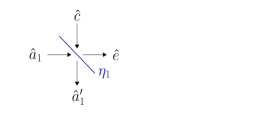
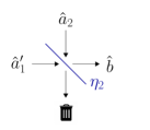
Figure 2: The beam splitter relation of the single-mode bosonic MAC. The left beam splitter corresponds to the cribbing channel $\mathcal{L}_{A_{1}\to A_{1}^{\prime}E}$, while the right beam splitter describes the communication channel $\mathcal{N}_{A_{1}^{\prime}A_{2}\to B}$. Alice 1 encodes the message $m_{1}$ by a coherent state, and sends her transmission through $n$ uses of the cribbing channel $\mathcal{L}_{A_{1}\to A_{1}^{\prime}E}$. The output $E^{n}$ is the cribbing system which will be measured by the second transmitter in a strictly-causal manner. At time $i$, Alice 2 encodes a coherent state that depends on her message $m_{2}$ and on the previous cribbing measurement outcomes $z^{i-1}$, she sends the state, and then performs a measurement on $E^{i}$ to obtain a measurement outcome $z_{i}$ which she will use in the next time instance. The inputs $A_{1,i}^{\prime n}$ and $A_{2,i}$ are sent through the communication channel $\mathcal{N}_{A_{1}^{\prime}A_{2}\to B}$, and Bob receives the output $B_{i}$. Bob performs a measurement on $B^{n}$ to obtain an estimate $(\hat{m}_{1},\hat{m}_{2})$ of the senders’ messages.

IV-C Bosonic MAC with Strictly-Causal Cribbing

To demonstrate our results, consider the single-mode bosonic MAC. We extend the finite-dimension result in Theorem 4 to the bosonic channel with infinite-dimension Hilbert spaces based on the discretization limiting argument by Guha et al. [63]. A detailed description of (continuous-variable) bosonic systems can be found in [64]. Here, we only define the notation for the quantities that we use. We use hat-notation, e.g. $\hat{a}$, $\hat{b}$, $\hat{e}$, to denote operators that act on a quantum state. The single-mode Hilbert space is spanned by the Fock basis $\{|n\rangle\}_{n=0}^{\infty}$. Each $|n\rangle$ is an eigenstate of the number operator $\hat{n}=\hat{a}^{\dagger}\hat{a}$, where $\hat{a}$ is the bosonic field annihilation operator. In particular, $|0\rangle$ is the vacuum state of the field. The creation operator $\hat{a}^{\dagger}$ creates an excitation: $\hat{a}^{\dagger}|n\rangle=\sqrt{n+1}|n+1\rangle$, for $n\geq 0$. Reversely, the annihilation operator $\hat{a}$ takes away an excitation: $\hat{a}|n+1\rangle=\sqrt{n+1}|n\rangle$. A coherent state $|\alpha\rangle$, where $\alpha\in\mathbb{C}$, corresponds to an oscillation of the electromagnetic field, and it is the outcome of applying the displacement operator to the vacuum state, i.e. $|\alpha\rangle=D(\alpha)|0\rangle$, which resembles the creation operation, with $D(\alpha)\equiv\exp(\alpha\hat{a}^{\dagger}-\alpha^{*}\hat{a})$. A thermal state $\tau(N)$ is a Gaussian mixture of coherent states, where

$$\tau(N) \equiv\int_{\mathbb{C}}d^{2}\alpha\frac{e^{-|\alpha|^{2}/N}}{\pi N}|\alpha\rangle\langle\alpha|$$

$$=\frac{1}{N+1}\sum_{n=0}^{\infty}\left(\frac{N}{N+1}\right)^{n}|n\rangle\langle n|$$ (53)

given an average photon number $N\geq 0$.

Consider a bosonic MAC with cribbing encoders, whereby the channel input is a pair of electromagnetic field modes, with annihilation operator $\hat{a}_{1}$ and $\hat{a}_{2}$, and the output is a modes with annihilation operator $\hat{b}$. The annihilation operators correspond to Alice 1, Alice 2, and Bob, respectively. The input-output relation of the bosonic MAC in the Heisenberg picture [65] is given by

$$\hat{e} =\sqrt{\eta_{1}}\,\hat{a}_{1}+\sqrt{1-\eta_{1}}\,\hat{c}$$ (54)

$$\hat{a}_{1}^{\prime} =\sqrt{1-\eta_{1}}\,\hat{a}_{1}-\sqrt{\eta_{1}}\,\hat{c}$$ (55)

and

$$\hat{b} =\sqrt{\eta_{2}}\,\hat{a}_{1}^{\prime}+\sqrt{1-\eta_{2}}\,\hat{a}_{2}$$ (56)

where $\hat{c}$ is associated with the environment noise and the parameter $\eta_{k}$ is the transmissivity, $0\leq\eta_{k}\leq 1$, which captures, for instance, the length of the optical fiber and its absorption length [66]. The relations above correspond to the outputs of a beam splitter, as illustrated in Figure 2. It is assumed that the encoder uses a coherent state protocol with an input constraint. That is, the input state is a coherent state $|x_{k}\rangle$, $x_{k}\in\mathbb{C}$, for $k=1,2$, such that each codeword satisfies $\frac{1}{n}\sum_{i=1}^{n}|x_{k,i}|^{2}\leq N_{A_{k}}$.

Based on part 1 of Theorem 4, we derive the following achievable region with strictly-causal cribbing,

$$\mathcal{C}_{\text{s-c}}(\mathcal{N}\circ\mathcal{L})\supseteq\left\{\begin{array}[]{rrl}(R_{1},R_{2})\,:&R_{1}&\leq g(\eta_{1}N_{A_{1}}+(1-\eta_{1})N_{C})-g((1-\eta_{1})N_{C})\\ &R_{2}&\leq g(\eta_{2}\eta_{1}N_{C}+(1-\eta_{2})N_{A_{2}})-g(\eta_{2}\eta_{1}N_{C})\\ &R_{1}+R_{2}&\leq g(\eta_{2}(1-\eta_{1})N_{A_{1}}+\eta_{2}\eta_{1}N_{C}+(1-\eta_{2})N_{A_{2}})-g(\eta_{2}\eta_{1}N_{C})\end{array}\right\}$$ (60)

where $$g(N) N$$ is the entropy of a thermal state with mean photon number ,

$$g(x) =\begin{cases}(x+1)\log(x+1)-x\log(x)&x>0\\ 0&x=0\,.\end{cases}$$ (61)

To obtain the region above, set the inputs to be mixed coherent states, $|X_{1}\rangle$ and $|X_{2}\rangle$, where $X_{k}$ is a circularly-symmetric Gaussian random variable with zero mean and variance $N_{A_{k}}/2$, for $k=1,2$, and let $U=0$.

On the other hand, the capacity region of single-mode Bosonic MAC without cribbing is [67]

$$\mathcal{C}_{\text{none}}(\mathcal{N}\circ\mathcal{L})=\left\{\begin{array}[]{rrl}(R_{1},R_{2})\,:&R_{1}&\leq g(\eta_{2}(1-\eta_{1})N_{A_{1}}+\eta_{2}\eta_{1}N_{C})-g(\eta_{2}\eta_{1}N_{C})\\ &R_{2}&\leq g(\eta_{2}\eta_{1}N_{C}+(1-\eta_{2})N_{A_{2}})-g(\eta_{2}\eta_{1}N_{C})\\ &R_{1}+R_{2}&\leq g(\eta_{2}(1-\eta_{1})N_{A_{1}}+\eta_{2}\eta_{1}N_{C}+(1-\eta_{2})N_{A_{2}})-g(\eta_{2}\eta_{1}N_{C})\end{array}\right\}\,.$$ (65)

The decode-forward achievable region with strictly-causal cribbing and the capacity region without cribbing are depicted in Figure 3 as the area below the thick blue line and below the dashed red line, respectively. As can be seen in the figure, cribbing can lead to a significant rate gain for Alice 1.

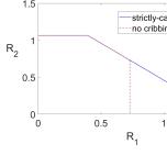
Figure 3: Achievable regions for the single-mode bosonic MAC. The decode forward achievable region with strictly-causal cribbing is the area below the thick blue line (see (60)). For comparison, the capacity region without cribbing $\mathcal{C}_{\text{none}}(\mathcal{N}\circ\mathcal{L})$ is depicted as the area below the red dashed line (see (65)). The transmission rate of Alice 1 can be significantly higher using cribbing.

V Partial Decode-Forward

We have pointed out in Remark 5 that if the cribbing system is not robust, then the decode-forward strategy in the previous section is not necessarily optimal. In fact, if the cribbing system $E$ that Alice 2 measures is noisier than the channel input $A_{1}^{\prime}$, then the inner bounds above may be worse than in transmission without cribbing. This is easy to see when $E$ does not contain any information, say $|\mathcal{H}_{E}|=1$, in which case the decode-forward region leaves Alice 1 with zero rate,

$$\mathcal{R}^{\text{DF}}_{\text{s-c}}(\mathcal{N}\circ\mathcal{L})=\mathcal{R}^{\text{DF}}_{\text{caus}}(\mathcal{N}\circ\mathcal{L})=\Big{\{}(0,R_{2})\,:\;R_{2}\leq\max_{p_{X}\,,\;\zeta_{A_{2}}^{x}}I(X;B)\Big{\}}\,.$$ (66)

In order to treat the case where the cribbing system is noisy, we introduce a quantum cribbing method that is based on relay coding techniques (see Remark 2 on the analogy between the relay channel and the cribbing model). Specifically, we improve the inner bound by incorporating the partial decode-forward technique within our previous cribbing scheme. Consider the quantum MAC with strictly-causal cribbing. Define

$$\mathcal{R}^{\text{PDF}}_{\text{s-c}}(\mathcal{N}\circ\mathcal{L})=\bigcup_{p_{UV}p_{X_{1}|U,V}p_{X_{2}|U,V}\,,\;\theta_{A_{1}}^{x_{1}}\otimes\zeta_{A_{2}}^{x_{2}}}\left\{\begin{array}[]{rl}(R_{1},R_{2})\,:\;R_{1}&\leq I(V;E|U)_{\omega}+I(X_{1};B|X_{2}UV)_{\omega}\\ R_{2}&\leq I(X_{2};B|X_{1}U)_{\omega}\\ R_{1}+R_{2}&\leq I(X_{1}X_{2};B)_{\omega}\end{array}\right\}$$ (70)

with

$$\omega_{UVX_{1}X_{2}A_{1}^{\prime}EA_{2}}=\sum_{u,v,x_{1},x_{2}}p_{U,V}(u,v)p_{X_{1}|U,V}(x_{1}|u,v)p_{X_{2}|U,V}(x_{2}|u,v)|u,v,x_{1},x_{2}\rangle\langle u,v,x_{1},x_{2}|\otimes\mathcal{L}_{A_{1}\to A_{1}^{\prime}E}(\theta_{A_{1}}^{x_{1}})\otimes\zeta_{A_{2}}^{x_{2}}\,,$$ (71)

$$\omega_{UVX_{1}X_{2}B}=\mathcal{N}_{A_{1}^{\prime}A_{2}\to B}(\omega_{UVX_{1}X_{2}A_{1}^{\prime}A_{2}})\,.$$ (72)

The superscript ‘PDF’ stands for partial decode-forward coding.

Theorem 7.

Consider a quantum MAC $\mathcal{N}_{A_{1}^{\prime}A_{2}\to B}\circ\mathcal{L}_{A_{1}\to A_{1}^{\prime}E}$. The rate region $\mathcal{R}^{\text{PDF}}_{\text{s-c}}(\mathcal{N}\circ\mathcal{L})$ is achievable for the quantum MAC with strictly-causal cribbing, i.e.

$$\mathcal{C}_{\text{s-c}}(\mathcal{N}\circ\mathcal{L})\supseteq\mathcal{R}^{\text{PDF}}_{\text{s-c}}(\mathcal{N}\circ\mathcal{L})\,.$$ (73)

The proof of Theorem 7 is given in Appendix F. To the best of our knowledge, this is a new result for classical channels as well. As opposed to the analysis for Section IV, the decoder does not fully rely on the cribbing measurement to recover the information from Alice 1. Instead, we use rate-splitting such that part of Alice 1’s message is decoded-forward through the cribbing system $E$, and the remaining part is decoded using $A_{1}^{\prime}$.

For the classical-quantum MAC with noisy cribbing, we also prove a cutset upper bound. In this case, the channel inputs are $A_{1}^{\prime}\equiv A_{1}\equiv X_{1}$ and $A_{2}\equiv X_{2}$, and the cribbing channel $\mathcal{L}$ is represented by a classical noisy channel $Q_{Z|X_{1}}$ (see Definition 3). Then, we determine the capacity region in the special case where $Z$ is a determinisitic function of $X_{1}$, by showing that the partial decode-forward inner bound and the cutset outer bound coincide. Given a classical-quantum MAC $\mathcal{N}_{X_{1}X_{2}\to B}\circ Q_{Z|X_{1}}$, define

$$\mathcal{R}^{\text{CS}}_{\text{s-c}}(\mathcal{N}\circ Q)=\bigcup_{p_{U}p_{X_{1}|U}p_{X_{2}|U}}\left\{\begin{array}[]{rl}(R_{1},R_{2})\,:\;R_{1}&\leq I(X_{1};BZ|X_{2}U)_{\omega}\\ R_{2}&\leq I(X_{2};B|X_{1}U)_{\omega}\\ R_{1}+R_{2}&\leq I(X_{1}X_{2};B)_{\omega}\end{array}\right\}$$ (77)

with

$$\omega_{UX_{1}X_{2}ZB}=\sum_{u,x_{1},z,x_{2}}p_{U}(u)p_{X_{1}|U}(x_{1}|u)Q_{Z|X_{1}}(z|x_{1})p_{X_{2}|U}(x_{2}|u)|u,x_{1},z,x_{2}\rangle\langle u,x_{1},z,x_{2}|\otimes\mathcal{N}_{X_{1}X_{2}\to B}(x_{1},x_{2})\,.$$ (78)

The superscript ‘CS’ stands for the cutset outer bound.

Theorem 8.

Consider a classical-quantum MAC with a noisy cribbing channel $Q_{Z|X_{1}}$.

1. The capacity region of the classical-quantum MAC $\mathcal{N}_{X_{1}X_{2}\to B}\circ Q_{Z|X_{1}}$ with strictly-causal noisy cribbing is bounded by

   $$\mathcal{C}_{\text{s-c}}(\mathcal{N}\circ Q)\subseteq\mathcal{R}^{\text{CS}}_{\text{s-c}}(\mathcal{N}\circ Q)\,.$$ (79)

2. If $Q_{Z|X_{1}}$ is a $0$-$1$ matrix, i.e. the cribbing observation $Z$ is a deterministic function of $X_{1}$, then

   $$\mathcal{C}_{\text{s-c}}(\mathcal{N}\circ Q)=\mathcal{R}^{\text{PDF}}_{\text{s-c}}(\mathcal{N}\circ Q)=\mathcal{R}^{\text{CS}}_{\text{s-c}}(\mathcal{N}\circ Q)=\bigcup_{p_{U}p_{X_{1}|U}p_{X_{2}|U}}\left\{\begin{array}[]{l}(R_{1},R_{2})\,:\\ R_{1}\leq H(Z|U)+I(X_{1};B|X_{2}UZ)_{\omega}\\ R_{2}\leq I(X_{2};B|X_{1}U)_{\omega}\\ R_{1}+R_{2}\leq I(X_{1}X_{2};B)_{\omega}\end{array}\right\}\,.$$ (84)

The proof of Theorem 8 is given in Appendix G. Part 1 seems to be new for classical channels as well, while part 2 is the classical-quantum version of the classical result on the classical MAC with partial cribbing [37]. Although, Asnani and Permuter [37] considered a more complex network with cribbing at both encoders.

VI Summary and Discussion

We consider the quantum MAC $\mathcal{M}_{A_{1}A_{2}\to B}$ with cribbing encoders. In quantum communication, the description is more delicate. By the no-cloning theorem, universal copying of quantum states is impossible. Therefore, in the view of quantum mechanics, perfect cribbing is against the laws of nature. As illustrated in Figure 1, if Alice 1 sends $A_{1}$ through the channel, then Alice 2 is physically prohibited from having a copy of the input state. Hence, we consider the quantum MAC with noisy cribbing, consisting of a concatenation of a cribbing channel $\mathcal{L}_{A_{1}\to A_{1}^{\prime}E}$ and the communication channel $\mathcal{N}_{A_{1}^{\prime}A_{2}\to B}$ (see Figure 1b). Specifically, Alice 1 sends her input system $A_{1}$ through a cribbing channel that has two outputs, $A_{1}^{\prime}$ and $E$. Alice 2 performs a measurement on the system $E$, and uses the measurement outcome in order to encode the input state of $A_{2}$. Then, the input systems $A_{1}^{\prime}$ and $A_{2}$ are sent through the communication channel. The model can also be interpreted as if the second transmitter performs a measurement on the environment $E$ of the first transmitter.

We consider the scenarios of strictly-causal, causal, and non-causal cribbing. In strictly-causal cribbing, Alice 2 transmits $A_{2,i}$ at time $i$, and then measures the cribbing system $E_{i}$ after the transmission. Hence, she only knows the past measurement outcomes $z^{i-1}$ at time $i$. In the causal setting, Alice 2 measures the cribbing system $E_{i}$, at time $i$, before she transmits. Hence, she knows the past and present measurement outcomes $z^{i}=(z^{i-1},z_{i})$ at time $i$. Whereas, in the non-causal case, Alice 2 can perform a joint measurement on $E^{n}$ a priori, i.e. before the beginning of her transmission. The entanglement between Transmitter 1 and the cribbing system of Transmitter 2 has the following implication. In both the causal and non-causal scenarios, Alice 2 performs the measurement before the input $A_{1,i}^{\prime}$ is sent through the channel. Hence, the cribbing measurement may inflict a “state collapse” for Alice 1’s transmission. In other words, in quantum communication, the cribbing operation interferes with Alice 1’s input before it is even transmitted through the communication channel. For a MAC with robust cribbing, there exists a recovery channel from $E$ to $EA_{1}^{\prime}$. Thereby, the cribbing system $E$ includes all the information that is available in $A_{1}^{\prime}$. We derived achievable regions for each setting and established a regularized capacity characterization for robust cribbing.

The setting of noisy cribbing is significantly more challenging and it is closely-related to the relay channel. We have derived a generalized packing lemma for the MAC. While the lemma does not include cribbing, it is useful in the analysis of the MAC with cribbing encoders. In the setting of the generalized quantum packing lemma in Section III, Alice 1 and Alice 2 send three messages to Bob, a common message $m_{0}$ and two private messages $m_{1}$ and $m_{2}$. It is assumed that there is no cribbing. The generalized quantum packing lemma implies that the capacity region of the quantum MAC $\mathcal{M}_{A_{1}A_{2}\to B}$ with a common message, without cribbing, is given by the regularization of the following region,

$$\mathcal{R}_{\text{none}}^{*}(\mathcal{M})=\bigcup_{p_{U}p_{X_{1}|U}p_{X_{2}|U}\,,\;\theta_{A_{1}}^{x_{1}}\otimes\zeta_{A_{2}}^{x_{2}}}\left\{\begin{array}[]{rl}(R_{0},R_{1},R_{2})\,:\;R_{1}&\leq I(X_{1};B|X_{2}U)_{\omega}\\ R_{2}&\leq I(X_{2};B|X_{1}U)_{\omega}\\ R_{1}+R_{2}&\leq I(X_{1}X_{2};B|U)_{\omega}\\ R_{0}+R_{1}+R_{2}&\leq I(X_{1}X_{2};B)_{\omega}\end{array}\right\}$$ (89)

where the union is as in (14), with $|\mathcal{U}|=|\mathcal{H}_{A_{1}}|^{2}+|\mathcal{H}_{A_{2}}|^{2}+1$, $|\mathcal{X}_{1}|\leq|\mathcal{U}|(|\mathcal{H}_{A_{k}}|^{2}+1)$, for $k=1,2$. This generalizes the classical-quantum result due to Boche and Nötzel [17, Theorem 2].

We further investigated the comparison between the relay channel and the MAC with cribbing encoders in Section V (see Remark 2). Building on the analogy between the noisy cribbing model and the relay channel, we developed a partial decode-forward region for the quantum MAC with strictly-causal non-robust cribbing. For the classical-quantum MAC with cribbing encoders, we have completely determined the capacity region with perfect cribbing of the classical input, and derived a cutset region for noisy cribbing. In the special case of a classical-quantum MAC with a deterministic cribbing channel, the inner and outer bounds coincide.

Cooperation in terms of a quantum MAC offers additional advantages for resilience and trustworthiness, e.g. to compensate for jamming attacks by an adversary [68, Section VI.C.]. As previously mentioned, in future communication systems, not only data but also physical and virtual objects will be controlled [31]. This growing demand of communication resources sharpens the need for quantum technology, and it is thus interesting to develop the corresponding theory.

Appendix A Proof of Lemma 2 (Generalized Quantum Packing Lemma)

Consider the following code construction and decoding measurement.

Classical Codebook Construction

 

1. Generate $2^{nR_{0}}$ independent sequences $u^{n}(m_{0})$, $m_{0}\in[1:2^{nR_{0}}]$, at random according to $\prod_{i=1}^{n}p_{U}(u_{i})$.

2. For every $m_{0}$, generate $2^{nR_{k}}$ conditionally independent sequences $x_{k}^{n}(m_{0},m_{k})$, $m_{k}\in[1:2^{nR_{k}}]$, according to $\prod_{i=1}^{n}p_{X_{k}|U}(x_{k,i}|u_{i}(m_{0}))$, where $k=1,2$.

We denote the codebooks by $\mathscr{C}=(\mathscr{C}_{0},\mathscr{C}_{1},\mathscr{C}_{2})$, respectively.

Decoding POVM

For every $u^{n},x_{1}^{n},x_{2}^{n}$, define

$$\Upsilon_{u^{n}x_{1}^{n}x_{2}^{n}}=\Pi\Pi_{u^{n}}\Pi_{u^{n}x_{1}^{n}}\Pi_{u^{n}x_{2}^{n}}\Pi_{u^{n}x_{1}^{n}x_{2}^{n}}\Pi_{u^{n}x_{2}^{n}}\Pi_{u^{n}x_{1}^{n}}\Pi_{u^{n}}\Pi\,.$$ (90)

Then, define

$$\Lambda_{m_{0},m_{1},m_{2}}=$$

$$\left(\sum_{m_{0}^{\prime}=1}^{2^{nR_{0}}}\sum_{m_{1}^{\prime}=1}^{2^{nR_{1}}}\sum_{m_{2}^{\prime}=1}^{2^{nR_{2}}}\Upsilon_{u^{n}(m_{0}^{\prime})x_{1}^{n}(m_{0}^{\prime},m_{1}^{\prime})x_{2}^{n}(m_{0}^{\prime},m_{2}^{\prime})}\right)^{-1/2}$$

$$\cdot\Upsilon_{u^{n}(m_{0})x_{1}^{n}(m_{0},m_{1})x_{2}^{n}(m_{0},m_{2})}$$

$$\cdot\left(\sum_{m_{0}^{\prime}=1}^{2^{nR_{0}}}\sum_{m_{1}^{\prime}=1}^{2^{nR_{1}}}\sum_{m_{2}^{\prime}=1}^{2^{nR_{2}}}\Upsilon_{u^{n}(m_{0}^{\prime})x_{1}^{n}(m_{0}^{\prime},m_{1}^{\prime})x_{2}^{n}(m_{0}^{\prime},m_{2}^{\prime})}\right)^{-1/2}\,.$$ (91)

Error Analysis

Denote the message-average error probability by

$$P_{e}^{(n)}(\mathscr{C}) =\frac{1}{2^{n(R_{0}+R_{1}+R_{2})}}\sum_{m_{0}^{\prime\prime},m_{1}^{\prime\prime},m_{2}^{\prime\prime}}P_{e}^{(n)}(\mathscr{C}|m_{0}^{\prime\prime},m_{1}^{\prime\prime},m_{2}^{\prime\prime})$$ (92)

where the conditional probability of error is defined as

$$P_{e}^{(n)}(\mathscr{C}|m_{0},m_{1},m_{2})\equiv\mathrm{Tr}\left[(\text{1}-\Lambda_{m_{0},m_{1},m_{2}})\rho_{U^{n}(m_{0}),X_{1}^{n}(m_{0},m_{1}),X_{2}^{n}(m_{0},m_{2})}\right]\,.$$ (93)

We will show that the expected probability of error is bounded by

$$\mathbb{E}_{\mathscr{C}}P_{e}^{(n)}(\mathscr{C})\leq 2(\alpha+3\sqrt{\alpha})+4\bigg{(}4\cdot 2^{-n(\mathsf{E}_{0}-\mathsf{e}_{0}-(R_{0}+R_{1}+R_{2})-\alpha)}$$

$$+2^{-n(\mathsf{E}_{1}-\mathsf{e}_{0}-R_{1}-\alpha)}+2^{-n(\mathsf{E}_{2}-\mathsf{e}_{0}-R_{2}-\alpha)}+2^{-n(\mathsf{E}_{12}-\mathsf{e}_{0}-(R_{1}+R_{2})-\alpha)}\bigg{)}\,.$$ (94)

Fix a message triplet $(m_{0},m_{1},m_{2})$. By the symmetry of the codebook generation, we have

$$\mathbb{E}_{\mathscr{C}}P_{e}^{(n)}(\mathscr{C})=\frac{1}{2^{n(R_{0}+R_{1}+R_{2})}}\sum_{m_{0}^{\prime\prime},m_{1}^{\prime\prime},m_{2}^{\prime\prime}}\mathbb{E}_{\mathscr{C}}P_{e}^{(n)}(\mathscr{C}|m_{0}^{\prime\prime},m_{1}^{\prime\prime},m_{2}^{\prime\prime})$$

$$=\mathbb{E}_{\mathscr{C}}P_{e}^{(n)}(\mathscr{C}|m_{0},m_{1},m_{2})\,.$$ (95)

Hence, we may assume without loss of generality that the triplet $(m_{0},m_{1},m_{2})$ was sent.

The error analysis begins with the Hayashi-Nagaoka inequality [69, Lemma 2],

$$\text{1}-(S_{1}+S_{2})^{-1/2}S_{1}(S_{1}+S_{2})^{-1/2}\leq 2(\text{1}-S_{1})+4S_{2}\,,$$ (96)

for $S_{1}$, $S_{2}$ such that $0\preceq S_{j}\preceq\text{1}$, $j=1,2$. Then, by the definition of $\Lambda_{m_{0},m_{1},m_{2}}$ in (91),

$$\text{1}-\Lambda_{m_{0},m_{1},m_{2}} \preceq 2(\text{1}-\Upsilon_{U^{n}(m_{0})X_{1}^{n}(m_{0},m_{1})X_{2}^{n}(m_{0},m_{2})})$$

$$+4\sum_{\begin{subarray}{c}m_{0}^{\prime},m_{1}^{\prime},m_{2}^{\prime}\,:\;\\ (m_{0}^{\prime},m_{1}^{\prime},m_{2}^{\prime})\neq(m_{0},m_{1},m_{2})\end{subarray}}\Upsilon_{U^{n}(m_{0}^{\prime})X_{1}^{n}(m_{0}^{\prime},m_{1}^{\prime})X_{2}^{n}(m_{0}^{\prime},m_{2}^{\prime})}\,.$$ (97)

Thus, the expected probability of error satisfies

$$\mathbb{E}_{\mathscr{C}}P_{e}^{(n)}(\mathscr{C}) =\mathbb{E}_{\mathscr{C}}P_{e}^{(n)}(\mathscr{C}|m_{0},m_{1},m_{2})$$

$$\leq 2\mathbb{E}\bigg{\{}\mathrm{Tr}\big{[}(\text{1}-\Upsilon_{U^{n}(m_{0}),X_{1}^{n}(m_{0},m_{1}),X_{2}^{n}(m_{0},m_{2})})\cdot\rho_{U^{n}(m_{0}),X_{1}^{n}(m_{0},m_{1}),X_{2}^{n}(m_{0},m_{2})}\big{]}\bigg{\}}$$

$$+4\sum_{\begin{subarray}{c}m_{0}^{\prime},m_{1}^{\prime},m_{2}^{\prime}\,:\;(m_{0}^{\prime},m_{1}^{\prime},m_{2}^{\prime})\neq(m_{0},m_{1},m_{2})\end{subarray}}\mathbb{E}\bigg{\{}\mathrm{Tr}\big{[}\Upsilon_{U^{n}(m_{0}^{\prime}),X_{1}^{n}(m_{0}^{\prime},m_{1}^{\prime}),X_{2}^{n}(m_{0}^{\prime},m_{2}^{\prime})}\cdot\rho_{U^{n}(m_{0}),X_{1}^{n}(m_{0},m_{1}),X_{2}^{n}(m_{0},m_{2})}\big{]}\bigg{\}}$$ (98)

where the equality is due to (95), and the inequality follows from (93) and (97).

The first term is now bounded as in the single-user case [15]. We note that the probability that $(U^{n}(m_{0}),X_{1}^{n}(m_{0},m_{1}),X_{2}^{n}(m_{0},m_{2}))$ is not $\delta$-typical, for our fixed message triplet $(m_{0},m_{1},m_{2})$, tends to zero as $n\rightarrow\infty$, by the weak law of large numbers. That is,

$$\Pr\Big{(}U^{n}(m_{0}),X_{1}^{n}(m_{0},m_{1}),X_{2}^{n}(m_{0},m_{2})\notin\mathcal{A}^{\delta}(P_{U}P_{X_{1}|U}P_{X_{2}})\Big{)}\leq\zeta_{n}$$ (99)

where $\zeta_{n}$ tends to zero as $n\to\infty$. For every $\delta$-typical realization of $(u^{n}(m_{0}),x_{1}^{n}(m_{0},m_{1}),x_{2}^{n}(m_{0},m_{2}))$, we have

$$\mathrm{Tr}\big{[}\Upsilon_{u^{n}(m_{0}),x_{1}^{n}(m_{0},m_{1}),x_{2}^{n}(m_{0},m_{2})}\cdot\rho_{u^{n}(m_{0}),x_{1}^{n}(m_{0},m_{1}),x_{2}^{n}(m_{0},m_{2})}\big{]}$$

$$=\mathrm{Tr}\big{[}\Pi\Pi_{u^{n}}\Pi_{u^{n}x_{1}^{n}}\Pi_{u^{n}x_{2}^{n}}\Pi_{u^{n}x_{1}^{n}x_{2}^{n}}\Pi_{u^{n}x_{2}^{n}}\Pi_{u^{n}x_{1}^{n}}\Pi_{u^{n}}\Pi\cdot\rho_{u^{n},x_{1}^{n},x_{2}^{n}}\big{]}$$ (100)

with $u^{n}\equiv u^{n}(m_{0})$, $x_{1}^{n}\equiv x_{1}^{n}(m_{0},m_{1})$, and $x_{2}^{n}\equiv x_{2}^{n}(m_{0},m_{2})$. Then, by the cyclicity of the trace operation, this equals

$$\mathrm{Tr}\big{[}\Pi_{u^{n}}\Pi_{u^{n}x_{1}^{n}}\Pi_{u^{n}x_{2}^{n}}\Pi_{u^{n}x_{1}^{n}x_{2}^{n}}\Pi_{u^{n}x_{2}^{n}}\Pi_{u^{n}x_{1}^{n}}\Pi_{u^{n}}\cdot\Pi\rho_{u^{n},x_{1}^{n},x_{2}^{n}}\Pi\big{]}$$

$$\geq\mathrm{Tr}\big{[}\Pi_{u^{n}}\Pi_{u^{n}x_{1}^{n}}\Pi_{u^{n}x_{2}^{n}}\Pi_{u^{n}x_{1}^{n}x_{2}^{n}}\Pi_{u^{n}x_{2}^{n}}\Pi_{u^{n}x_{1}^{n}}\Pi_{u^{n}}\cdot\rho_{u^{n},x_{1}^{n},x_{2}^{n}}\big{]}-\big{\lVert}\Pi\rho_{u^{n},x_{1}^{n},x_{2}^{n}}\Pi-\rho_{u^{n},x_{1}^{n},x_{2}^{n}}\big{\rVert}$$

$$\geq\mathrm{Tr}\big{[}\Pi_{u^{n}}\Pi_{u^{n}x_{1}^{n}}\Pi_{u^{n}x_{2}^{n}}\Pi_{u^{n}x_{1}^{n}x_{2}^{n}}\Pi_{u^{n}x_{2}^{n}}\Pi_{u^{n}x_{1}^{n}}\Pi_{u^{n}}\cdot\rho_{u^{n},x_{1}^{n},x_{2}^{n}}\big{]}-2\sqrt{\alpha}$$ (101)

where the last inequality follows from the gentle operator lemma [70] [56, Lemma 9.4.2] and Assumption (a). Repeating this argument for $\Pi_{u^{n}}$, $\Pi_{u^{n}x_{1}^{n}}$, $\Pi_{u^{n}x_{2}^{n}}$, using Assumptions (b), (c), (d), respectively, we have

$$\mathrm{Tr}\big{[}\Pi_{u^{n}}\Pi_{u^{n}x_{1}^{n}}\Pi_{u^{n}x_{2}^{n}}\Pi_{u^{n}x_{1}^{n}x_{2}^{n}}\Pi_{u^{n}x_{2}^{n}}\Pi_{u^{n}x_{1}^{n}}\Pi_{u^{n}}\cdot\rho_{u^{n},x_{1}^{n},x_{2}^{n}}\big{]}$$

$$\geq\mathrm{Tr}\big{[}\Pi_{u^{n}x_{1}^{n}x_{2}^{n}}\cdot\rho_{u^{n},x_{1}^{n},x_{2}^{n}}\big{]}-6\sqrt{\alpha}$$

$$\geq 1-\alpha-6\sqrt{\alpha}$$ (102)

where the last inequality holds by Assumption (e). It follows that the first term in the RHS of (98) is bounded by $2(\alpha+6\sqrt{\alpha})+\zeta_{n}\leq 2(\alpha+7\sqrt{\alpha})$ (see (99)), for sufficiently large $n$.

Next, observe that the sum in the RHS of (98) can be divided as follows,

$$\sum_{\begin{subarray}{c}m_{0}^{\prime},m_{1}^{\prime},m_{2}^{\prime}\,:\;\\ (m_{0}^{\prime},m_{1}^{\prime},m_{2}^{\prime})\neq(m_{0},m_{1},m_{2})\end{subarray}}\mathbb{E}\mathrm{Tr}\Big{[}\Upsilon_{m_{0}^{\prime},m_{1}^{\prime},m_{2}^{\prime}}\cdot\rho_{U^{n}(m_{0}),X_{1}^{n}(m_{0},m_{1}),X_{2}^{n}(m_{0},m_{2})}\Big{]}$$

$$=\sum_{m_{0}^{\prime}\neq m_{0}}\mathbb{E}\mathrm{Tr}\Big{[}\Upsilon_{m_{0}^{\prime},m_{1},m_{2}}\rho_{U^{n}(m_{0}),X_{1}^{n}(m_{0},m_{1}),X_{2}^{n}(m_{0},m_{2})}\Big{]}$$

$$+\sum_{m_{1}^{\prime}\neq m_{1}}\mathbb{E}\mathrm{Tr}\Big{[}\Upsilon_{m_{0},m_{1}^{\prime},m_{2}}\rho_{U^{n}(m_{0}),X_{1}^{n}(m_{0},m_{1}),X_{2}^{n}(m_{0},m_{2})}\Big{]}$$

$$+\sum_{m_{2}^{\prime}\neq m_{2}}\mathbb{E}\mathrm{Tr}\Big{[}\Upsilon_{m_{0},m_{1},m_{2}^{\prime}}\rho_{U^{n}(m_{0}),X_{1}^{n}(m_{0},m_{1}),X_{2}^{n}(m_{0},m_{2})}\Big{]}$$

$$+\sum_{m_{1}^{\prime}\neq m_{1}\,,\;m_{2}^{\prime}\neq m_{2}}\mathbb{E}\mathrm{Tr}\Big{[}\Upsilon_{m_{0},m_{1}^{\prime},m_{2}^{\prime}}\rho_{U^{n}(m_{0}),X_{1}^{n}(m_{0},m_{1}),X_{2}^{n}(m_{0},m_{2})}\Big{]}$$

$$+\sum_{m_{0}^{\prime}\neq m_{0}\,,\;m_{1}^{\prime}\neq m_{1}}\mathbb{E}\mathrm{Tr}\Big{[}\Upsilon_{m_{0}^{\prime},m_{1}^{\prime},m_{2}}\cdot\rho_{U^{n}(m_{0}),X_{1}^{n}(m_{0},m_{1}),X_{2}^{n}(m_{0},m_{2})}\Big{]}$$

$$+\sum_{m_{0}^{\prime}\neq m_{0}\,,\;m_{2}^{\prime}\neq m_{2}}\mathbb{E}\mathrm{Tr}\Big{[}\Upsilon_{m_{0}^{\prime},m_{1},m_{2}^{\prime}}\cdot\rho_{U^{n}(m_{0}),X_{1}^{n}(m_{0},m_{1}),X_{2}^{n}(m_{0},m_{2})}\Big{]}$$

$$+\sum_{m_{0}^{\prime}\neq m_{0}\,,\;m_{1}^{\prime}\neq m_{1}\,,\;m_{2}^{\prime}\neq m_{2}}\mathbb{E}\mathrm{Tr}\Big{[}\Upsilon_{m_{0}^{\prime},m_{1}^{\prime},m_{2}^{\prime}}\cdot\rho_{U^{n}(m_{0}),X_{1}^{n}(m_{0},m_{1}),X_{2}^{n}(m_{0},m_{2})}\Big{]}$$ (103)

The derivation above is analogous to the union of events bound in the classical proof. In particular, the first three sums correspond to the event that exactly one of the messages is decoded erroneously, the next three sums to the event that two of the messages are decoded incorrectly, and the last sum is the probability that all of the decoder’s estimates are wrong.

Now, we will bound each of the seven sums in the RHS of (103). Consider the first sum. Then,

$$\mathbb{E}\mathrm{Tr}\Big{[}\Upsilon_{U^{n}(m_{0}^{\prime}),X_{1}^{n}(m_{0}^{\prime},m_{1}),X_{2}^{n}(m_{0}^{\prime},m_{2})}\rho_{U^{n}(m_{0}),X_{1}^{n}(m_{0},m_{1}),X_{2}^{n}(m_{0},m_{2})}\Big{]}$$

$$\leq\mathrm{Tr}\Big{[}\mathbb{E}\big{\{}\Pi\Pi_{U^{n}(m_{0}^{\prime}),X_{1}^{n}(m_{0}^{\prime},m_{1}),X_{2}^{n}(m_{0}^{\prime},m_{2})}\Pi\rho_{U^{n}(m_{0}),X_{1}^{n}(m_{0},m_{1}),X_{2}^{n}(m_{0},m_{2})}\big{\}}\Big{]}\,.$$ (104)

Observe that for every $m_{0}^{\prime}\neq m_{0}$, the random vectors $(U^{n}(m_{0}^{\prime}),X_{1}^{n}(m_{0}^{\prime},m_{1}),X_{2}^{n}(m_{0}^{\prime},m_{2}))$ and $(U^{n}(m_{0}),X_{1}^{n}(m_{0},m_{1}),X_{2}^{n}(m_{0},m_{2}))$ are statistically independent of each other. Thus, the expression in the square brackets becomes

$$\mathbb{E}\left\{\Pi\Pi_{U^{n}(m_{0}^{\prime}),X_{1}^{n}(m_{0}^{\prime},m_{1}),X_{2}^{n}(m_{0}^{\prime},m_{2})}\Pi\right\}\cdot\mathbb{E}\left\{\rho_{U^{n}(m_{0}),X_{1}^{n}(m_{0},m_{1}),X_{2}^{n}(m_{0},m_{2})}\right\}$$

$$=\mathbb{E}\left\{\Pi\Pi_{U^{n}(m_{0}^{\prime}),X_{1}^{n}(m_{0}^{\prime},m_{1}),X_{2}^{n}(m_{0}^{\prime},m_{2})}\Pi\right\}\cdot\rho^{\otimes n}\,.$$ (105)

Furthermore, the probability that one of the aforementioned random vectors is not $\delta$-typical tends to zero as $n\to\infty$, by the weak law of large numbers. It follows that

$$\mathbb{E}\mathrm{Tr}\Big{[}\Upsilon_{U^{n}(m_{0}^{\prime}),X_{1}^{n}(m_{0}^{\prime},m_{1}),X_{2}^{n}(m_{0}^{\prime},m_{2})}\cdot\rho_{U^{n}(m_{0}),X_{1}^{n}(m_{0},m_{1}),X_{2}^{n}(m_{0},m_{2})}\Big{]}$$

$$\leq\mathrm{Tr}\left[\mathbb{E}\left\{\Pi\Pi_{U^{n}(m_{0}^{\prime}),X_{1}^{n}(m_{0}^{\prime},m_{1}),X_{2}^{n}(m_{0}^{\prime},m_{2})}\Pi\right\}\cdot\rho^{\otimes n}\right]$$

$$=\mathbb{E}\mathrm{Tr}\left[\Pi\Pi_{U^{n}(m_{0}^{\prime}),X_{1}^{n}(m_{0}^{\prime},m_{1}),X_{2}^{n}(m_{0}^{\prime},m_{2})}\Pi\cdot\rho^{\otimes n}\right]$$

$$=\mathbb{E}\mathrm{Tr}\left[\Pi_{U^{n}(m_{0}^{\prime}),X_{1}^{n}(m_{0}^{\prime},m_{1}),X_{2}^{n}(m_{0}^{\prime},m_{2})}\cdot\Pi\rho^{\otimes n}\Pi\right]$$

$$\leq 2^{-n(\mathsf{E}_{0}-2\alpha)}\mathbb{E}\mathrm{Tr}\left[\Pi_{U^{n}(m_{0}^{\prime}),X_{1}^{n}(m_{0}^{\prime},m_{1}),X_{2}^{n}(m_{0}^{\prime},m_{2})}\cdot\Pi\right]$$

$$\leq 2^{-n(\mathsf{E}_{0}-2\alpha)}\mathbb{E}\mathrm{Tr}\left[\Pi_{U^{n}(m_{0}^{\prime}),X_{1}^{n}(m_{0}^{\prime},m_{1}),X_{2}^{n}(m_{0}^{\prime},m_{2})}\right]$$

$$\leq 2^{-n(\mathsf{E}_{0}-\mathsf{e}_{0}-3\alpha)}$$ (106)

where the second and last inequalities hold by Assumptions (f) and (g). Thus, for large $n$, the first sum in the RHS of (103) is bounded by $2^{-n(\mathsf{E}_{0}-\mathsf{e}_{0}-3\alpha)}\cdot 2^{nR_{0}}=2^{-n(\mathsf{E}_{0}-\mathsf{e}_{0}-R_{0}-3\alpha)}$. By the same considerations, the last three sums are bounded by $2^{-n(\mathsf{E}_{0}-\mathsf{e}_{0}-(R_{0}+R_{1})-3\alpha)}$, $2^{-n(\mathsf{E}_{0}-\mathsf{e}_{0}-(R_{0}+R_{2})-3\alpha)}$, and $2^{-n(\mathsf{E}_{0}-\mathsf{e}_{0}-(R_{0}+R_{1}+R_{2})-3\alpha)}$, respectively. Thus, the combination of the first, fifth, sixth, and seventh sums in the RHS of (103) is bounded by $4\cdot 2^{-n(\mathsf{E}_{0}-\mathsf{e}_{0}-(R_{0}+R_{1}+R_{2})-3\alpha)}$.

It remains to bound the second, third, and fourth sums in the RHS of (103). Moving to the second sum,

$$\mathbb{E}\mathrm{Tr}\Big{[}\Upsilon_{U^{n}(m_{0}),X_{1}^{n}(m_{0},m_{1}^{\prime}),X_{2}^{n}(m_{0},m_{2})}\cdot\rho_{U^{n}(m_{0}),X_{1}^{n}(m_{0},m_{1}),X_{2}^{n}(m_{0},m_{2})}\Big{]}$$

$$\leq\mathrm{Tr}\Big{[}\mathbb{E}\big{\{}\Pi_{U^{n}(m_{0}),X_{2}^{n}(m_{0},m_{2})}\Pi_{U^{n}(m_{0}),X_{1}^{n}(m_{0},m_{1}^{\prime}),X_{2}^{n}(m_{0}^{\prime},m_{2})}\Pi_{U^{n}(m_{0}),X_{2}^{n}(m_{0},m_{2})}\cdot\rho_{U^{n}(m_{0}),X_{1}^{n}(m_{0},m_{1}),X_{2}^{n}(m_{0},m_{2})}\big{\}}\Big{]}\,.$$ (107)

Consider a given realization of the codebooks $\mathscr{C}_{0}=\{u^{n}(m_{0})\}$ and $\mathscr{C}_{2}=\{x_{2}^{n}(m_{0},m_{1})\}$. For every $m_{1}^{\prime}\neq m_{1}$, the sequences $X_{1}^{n}(m_{0},m_{1}^{\prime})$ and $X_{1}^{n}(m_{0},m_{1})$ are statistically independent. Thus, when we condition on $\mathscr{C}_{0}$, $\mathscr{C}_{2}$, the expression in the square brackets becomes

$$\mathbb{E}_{\mathscr{C}_{1}}\left\{\Pi_{u^{n}(m_{0}),x_{2}^{n}(m_{0},m_{2})}\Pi_{u^{n}(m_{0}),X_{1}^{n}(m_{0},m_{1}^{\prime}),x_{2}^{n}(m_{0},m_{2})}\Pi_{u^{n}(m_{0}),x_{2}^{n}(m_{0},m_{2})}\right\}\cdot\mathbb{E}_{\mathscr{C}_{1}}\left\{\rho_{u^{n}(m_{0}),X_{1}^{n}(m_{0},m_{1}),x_{2}^{n}(m_{0},m_{2})}\right\}$$

$$=\mathbb{E}_{\mathscr{C}_{1}}\Big{\{}\Pi_{u^{n}(m_{0}),x_{2}^{n}(m_{0},m_{2})}\Pi_{u^{n}(m_{0}),X_{1}^{n}(m_{0},m_{1}^{\prime}),x_{2}^{n}(m_{0},m_{2})}\Pi_{u^{n}(m_{0}),x_{2}^{n}(m_{0},m_{2})}\Big{\}}\cdot\rho_{u^{n}(m_{0}),x_{2}^{n}(m_{0},m_{2})}\,.$$ (108)

It follows that

$$\mathbb{E}_{\mathscr{C}_{1}}\mathrm{Tr}\Big{[}\Upsilon_{u^{n}(m_{0}),X_{1}^{n}(m_{0},m_{1}^{\prime}),x_{2}^{n}(m_{0},m_{2})}\cdot\rho_{u^{n}(m_{0}),X_{1}^{n}(m_{0},m_{1}),x_{2}^{n}(m_{0},m_{2})}\Big{]}$$

$$\leq\mathrm{Tr}\Big{[}\mathbb{E}_{\mathscr{C}_{1}}\big{\{}\Pi_{u^{n}(m_{0}),x_{2}^{n}(m_{0},m_{2})}\Pi_{u^{n}(m_{0}),X_{1}^{n}(m_{0},m_{1}^{\prime}),x_{2}^{n}(m_{0},m_{2})}\Pi_{u^{n}(m_{0}),x_{2}^{n}(m_{0},m_{2})}\big{\}}\cdot\rho_{u^{n}(m_{0}),x_{2}^{n}(m_{0},m_{2})}\Big{]}$$

$$=\mathbb{E}_{\mathscr{C}_{1}}\mathrm{Tr}\Big{[}\Pi_{u^{n}(m_{0}),x_{2}^{n}(m_{0},m_{2})}\Pi_{u^{n}(m_{0}),X_{1}^{n}(m_{0},m_{1}^{\prime}),x_{2}^{n}(m_{0},m_{2})}\Pi_{u^{n}(m_{0}),x_{2}^{n}(m_{0},m_{2})}\cdot\rho_{u^{n}(m_{0}),x_{2}^{n}(m_{0},m_{2})}\Big{]}$$

$$=\mathbb{E}_{\mathscr{C}_{1}}\mathrm{Tr}\Big{[}\Pi_{u^{n}(m_{0}),X_{1}^{n}(m_{0},m_{1}^{\prime}),x_{2}^{n}(m_{0},m_{2})}\cdot\Pi_{u^{n}(m_{0}),x_{2}^{n}(m_{0},m_{2})}\rho_{u^{n}(m_{0}),x_{2}^{n}(m_{0},m_{2})}\Pi_{u^{n}(m_{0}),x_{2}^{n}(m_{0},m_{2})}\Big{]}$$

$$\leq 2^{-n(\mathsf{E}_{1}-2\alpha)}\mathbb{E}_{\mathscr{C}_{1}}\mathrm{Tr}\Big{[}\Pi_{u^{n}(m_{0}),X_{1}^{n}(m_{0},m_{1}^{\prime}),x_{2}^{n}(m_{0}^{\prime},m_{2})}\Pi_{u^{n}(m_{0}),x_{2}^{n}(m_{0},m_{2})}\Big{]}$$

$$\leq 2^{-n(\mathsf{E}_{1}-2\alpha)}\mathbb{E}_{\mathscr{C}_{1}}\mathrm{Tr}\left[\Pi_{u^{n}(m_{0}),X_{1}^{n}(m_{0},m_{1}^{\prime}),x_{2}^{n}(m_{0},m_{2}^{\prime})}\right]$$

$$\leq 2^{-n(\mathsf{E}_{1}-\mathsf{e}_{0}-3\alpha)}$$ (109)

by Assumptions (f) and (e). Thus, the second sum in the RHS of (103) is bounded by $2^{-n(\mathsf{E}_{1}-\mathsf{e}_{0}-3\alpha)}\cdot 2^{nR_{1}}=2^{-n(\mathsf{E}_{1}-\mathsf{e}_{0}-R_{1}-3\alpha)}$. By symmetry, the third sum is bounded by $2^{-n(\mathsf{E}_{2}-\mathsf{e}_{0}-R_{2}-3\alpha)}$.

As for the fourth sum in the RHS of (103),

$$\mathbb{E}\mathrm{Tr}\big{[}\Upsilon_{U^{n}(m_{0}),X_{1}^{n}(m_{0},m_{1}^{\prime}),X_{2}^{n}(m_{0},m_{2}^{\prime})}\cdot\rho_{U^{n}(m_{0}),X_{1}^{n}(m_{0},m_{1}),X_{2}^{n}(m_{0},m_{2})}\big{]}$$

$$\leq\mathrm{Tr}\Big{[}\mathbb{E}\big{\{}\Pi_{U^{n}(m_{0})}\Pi_{U^{n}(m_{0}),X_{1}^{n}(m_{0},m_{1}^{\prime}),X_{2}^{n}(m_{0},m_{2}^{\prime})}\Pi_{U^{n}(m_{0})}\cdot\rho_{U^{n}(m_{0}),X_{1}^{n}(m_{0},m_{1}),X_{2}^{n}(m_{0},m_{2})}\big{\}}\Big{]}$$ (110)

For every $m_{1}^{\prime}\neq m_{1}$ and $m_{2}^{\prime}\neq m_{2}$, the random vectors $(X_{1}^{n}(m_{0},m_{1}^{\prime}),X_{2}^{n}(m_{0},m_{2}^{\prime}))$ and $(X_{1}^{n}(m_{0},m_{1}),X_{2}^{n}(m_{0},m_{2}))$ are statistically independent. Thus, when we condition on $\mathscr{C}_{0}=\{u_{0}^{n}(m_{0})\}$, the expectation in the square bracket is a product,

$$\mathbb{E}_{\mathscr{C}_{1}\times\mathscr{C}_{2}}\left\{\Pi_{u^{n}(m_{0})}\Pi_{u^{n}(m_{0}),X_{1}^{n}(m_{0},m_{1}^{\prime}),X_{2}^{n}(m_{0},m_{2}^{\prime})}\Pi_{u^{n}(m_{0})}\right\}\cdot\mathbb{E}_{\mathscr{C}_{1}\times\mathscr{C}_{2}}\left\{\rho_{u^{n}(m_{0}),X_{1}^{n}(m_{0},m_{1}),X_{2}^{n}(m_{0},m_{2})}\right\}$$

$$=\mathbb{E}_{\mathscr{C}_{1}\times\mathscr{C}_{2}}\big{\{}\Pi_{u^{n}(m_{0})}\Pi_{u^{n}(m_{0}),X_{1}^{n}(m_{0},m_{1}^{\prime}),X_{2}^{n}(m_{0},m_{2}^{\prime})}\Pi_{u^{n}(m_{0})}\big{\}}\cdot\rho_{u^{n}(m_{0})}\,.$$ (111)

It follows that

$$\mathbb{E}_{\mathscr{C}_{1}\times\mathscr{C}_{2}}\mathrm{Tr}\big{[}\Upsilon_{u^{n}(m_{0}),X_{1}^{n}(m_{0},m_{1}^{\prime}),X_{2}^{n}(m_{0},m_{2}^{\prime})}\cdot\rho_{u^{n}(m_{0}),X_{1}^{n}(m_{0},m_{1}),X_{2}^{n}(m_{0},m_{2})}\big{]}$$

$$\leq 2^{-n(\mathsf{E}_{12}-2\alpha)}\mathbb{E}_{\mathscr{C}_{1}\times\mathscr{C}_{2}}\mathrm{Tr}\big{[}\Pi_{u^{n}(m_{0}),X_{1}^{n}(m_{0},m_{1}^{\prime}),X_{2}^{n}(m_{0},m_{2}^{\prime})}\Pi_{u^{n}(m_{0})}\big{]}$$

$$\leq 2^{-n(\mathsf{E}_{12}-\mathsf{e}_{0}-3\alpha)}$$ (112)

for sufficiently large $n$, by Assumptions (f) and (i).

We conclude that the probability of decoding error, averaged over the class of the codebooks, is bounded as in (94). Therefore, there must exist deterministic codebooks with the same error bound, as we were set to prove. ∎

Appendix B Proof of Lemma 3 (Cardinality Bounds)

To bound the alphabet size of the random variables $U$, $X_{1}$, and $X_{2}$, we use the Fenchel-Eggleston-Carathéodory lemma [61] and similar arguments as in [23, 57]. Let

$$d_{0} =|\mathcal{H}_{B}|^{2}+2$$ (113)

$$d_{1} =|\mathcal{U}|(|\mathcal{H}_{A_{1}}|^{2}+2)$$ (114)

$$d_{2} =|\mathcal{U}|(|\mathcal{H}_{A_{2}}|^{2}+1)\,.$$ (115)

First, we bound the cardinality of $\mathcal{U}$. Consider a given ensemble $\{p_{X_{1}|U}(x_{1}|u)p_{X_{2}|U}(x_{2}|u)\,,\theta_{A_{1}}^{x_{1}}\otimes\zeta_{A_{2}}^{x_{2}}\}$. Every density matrix $\rho_{A}$ has a unique parametric representation $\mathscr{V}(\rho_{A})$ of dimension $|\mathcal{H}_{A}|^{2}-1$. Then, define a map $f_{0}:\mathcal{U}\rightarrow\mathbb{R}^{d_{0}}$ by

$$f_{0}(u)=\Big{(}\mathscr{V}(\omega_{B}^{u})\,,\;H(B|X_{1},X_{2},U=u)_{\omega}\,,\;I(X_{1};E|U=u)_{\omega}\,,\;I(X_{2};B|X_{1}U=u)_{\omega}\Big{)}$$ (116)

where $\omega_{B}^{u}=\sum_{x_{1},x_{2}}p_{X_{1}|U}(x_{1}|u)p_{X_{2}|U}(x_{2}|u)$ $\mathcal{N}\left(\mathrm{Tr}_{E}\left(\mathcal{L}(\theta_{A_{1}}^{x_{1}})\right)\otimes\zeta_{A_{2}}^{x_{2}}\right)$. The map $f_{0}$ can be extended to a map that acts on probability distributions as follows,

$$F_{0}\,:\;p_{U}(\cdot)\mapsto\sum_{u\in\mathcal{U}}p_{U}(u)f_{0}(u)=\Big{(}\mathscr{V}(\omega_{B})\,,\;H(B|X_{1}X_{2})_{\omega}\,,\;I(X_{1};E|U)_{\omega}\,,\;I(X_{2};B|X_{1}U)_{\omega}\Big{)}\,.$$ (117)

According to the Fenchel-Eggleston-Carathéodory lemma [61], any point in the convex closure of a connected compact set within $\mathbb{R}^{d}$ belongs to the convex hull of $d$ points in the set. Since the map $F_{0}$ is linear, it maps the set of distributions on $\mathcal{U}$ to a connected compact set in $\mathbb{R}^{d_{0}}$. Thus, for every $p_{U}$, there exists a probability distribution $p_{\bar{U}}$ on a subset $\bar{\mathcal{U}}\subseteq\mathcal{U}$ of size $d_{0}$, such that $F_{0}(p_{{\bar{U}}})=F_{0}(p_{U})$. We deduce that alphabet size can be restricted to $|\mathcal{U}|\leq d_{0}$, while preserving $\omega_{B}$, $H(B|X_{1}X_{2})_{\omega}$, $I(X_{1};E|U)_{\rho}$, $I(X_{2};B|X_{1}U)_{\rho}$, and thus, $H(B)_{\omega}$ and $I(X_{1}X_{2};B)_{\omega}=H(B)_{\omega}-H(B|X_{1}X_{2})_{\omega}$.

Next, we bound the alphabet size for the auxiliary variables $X_{1}$ and $X_{2}$. For every $u\in\mathcal{U}$, define a map $f_{1,u}:\mathcal{X}_{1}\rightarrow\mathbb{R}^{|\mathcal{H}_{A_{1}}|^{2}+2}$ by

$$f_{1,u}(x_{1})=\Big{(}\mathscr{V}(\theta_{A_{1}}^{x_{1}})\,,\;H(E|X_{1}=x_{1},U=u)_{\omega}\,,\;H(B|X_{1}=x_{1},U=u)_{\omega}\,,\;H(B|X_{2},X_{1}=x_{1},U=u)_{\omega}\Big{)}\,.$$ (118)

Then, the map $f_{1}$ is extended to

$$F_{1,u}\,:\;p_{X_{1}|U}(\cdot|u)\mapsto \sum_{x_{1}\in\mathcal{X}_{1}}p_{X_{1}|U}(x_{1}|u)f_{1,u}(x_{1})=$$

$$\Big{(}\mathscr{V}(\theta^{u}_{A_{1}})\,,\;H(E|X_{1},U=u)\,,\;H(B|X_{1},U=u)_{\omega}\,,\;H(B|X_{2},X_{1},U=u)_{\omega}\Big{)}$$ (119)

with

$$\theta_{A_{1}}^{u}\equiv\sum_{x_{1}}p_{X_{1}|U}(x_{1}|u)\theta_{A_{1}}^{x_{1}}\,.$$ (120)

Thus, by Fenchel-Eggleston-Carathéodory lemma [61], for every $p_{X_{1}|U}(\cdot|u)$, there exists a probability distribution $p_{\bar{X}_{1}|U}(\cdot|u)$ on a subset $\bar{\mathcal{X}}_{1}\subseteq\mathcal{X}_{1}$ of size $|\mathcal{H}_{A_{1}}|^{2}+2$, such that $F_{1,u}(p_{{\bar{X}_{1}|U}}(\cdot|u))=F_{1,u}(p_{X_{1}|U}(\cdot|u)))$. We deduce that alphabet size can be restricted to $|\mathcal{X}_{1}|\leq d_{1}$, while preserving $H(E|X_{1}U)$, $H(B|X_{1}U)_{\omega}$, $H(B|X_{1}X_{2})_{\omega}$, and

$$\omega_{UA_{1}X_{2}A_{2}}=\sum_{u}p_{U}(u)p_{X_{2}|U}(x_{2}|u)|u\rangle\langle u|\otimes\theta_{A_{1}}^{u}\otimes|x_{2}\rangle\langle x_{2}|\otimes\zeta^{x_{2}}_{A_{2}}$$ (121)

where $\theta_{A_{1}}^{u}$ is as in (120). This implies that $\omega_{UA_{1}^{\prime}EX_{2}A_{2}}=\mathcal{L}(\omega_{UA_{1}X_{2}A_{2}})$, $H(E|U)_{\omega}$, and $I(X_{1};E|U)_{\omega}=H(E|U)_{\omega}-H(E|X_{1}U)_{\omega}$ remain the same, and also $\omega_{UX_{2}B}\equiv\mathcal{N}_{A_{1}^{\prime}A_{2}\rightarrow B}(\omega_{UX_{2}A_{1}^{\prime}A_{2}})$, $H(B)_{\omega}$, $I(X_{2};B|X_{1}U)_{\omega}=H(B|X_{1}U)_{\omega}-H(B|X_{1}X_{2})_{\omega}$, and $I(X_{1},X_{2};B)_{\omega}=H(B)_{\omega}-H(B|X_{1},X_{2})_{\omega}$. The bound $|\mathcal{X}_{2}|\leq d_{2}$ follows from the same argument using the function $f_{2,u}:\mathcal{X}_{2}\rightarrow\mathbb{R}^{|\mathcal{H}_{A_{2}}|^{2}+1}$,

$$f_{2,u}(x_{2})=\Big{(}\mathscr{V}(\zeta_{A_{2}}^{x_{2}})\,,\;H(B|X_{1},X_{2}=x_{2},U=u)_{\omega}\,,\;H(B|X_{1},X_{2}=x_{2})_{\omega}\Big{)}$$ (122)

for $u\in\mathcal{U}$. This completes the proof for the cardinality bounds. ∎

Appendix C Proof of Theorem 4

Consider the quantum MAC $\mathcal{N}\circ\mathcal{L}$ with strictly-causal cribbing.

Part 1

We show that for every $\delta_{1},\delta_{2},\varepsilon_{0}>0$, there exists a $(2^{n(R_{1}-\delta_{1})},2^{n(R_{2}-\delta_{2})},n,\varepsilon_{0})$ code for $\mathcal{N}_{A_{1}^{\prime}A_{2}\rightarrow B}\circ\mathcal{L}_{A_{1}\to A_{1}^{\prime}E}$ with strictly-causal cribbing at Encoder 2, provided that $(R_{1},R_{2})\in\mathcal{R}^{\text{DF}}_{\text{s-c}}(\mathcal{N}\circ\mathcal{L})$. To prove achievability, we extend the classical block Markov coding with backward decoding to the quantum setting, and then apply the quantum packing lemma.

We use $T$ transmission blocks, where each block consists of $n$ channel uses. In particular, with strictly-causal cribbing, Encoder 2 has access to the cribbing measurements from the previous blocks. Each transmitter sends $T-1$ messages. Let us fix $m_{k}(0)=m_{k}(T)\equiv 1$ for $k=1,2$. Alice 1 sends $(m_{1}(j))_{j=1}^{T-1}$, and Alice 2 $(m_{2}(j))_{j=1}^{T-1}$. Hence, the coding rate for User $k$ is $\left(\frac{T-1}{T}\right)R_{k}$, which tends to $R_{k}$ as the number of blocks $T$ grows to infinity.

Let $\{p_{U}(u)p_{X_{1}|U}(x_{1}|u)p_{X_{2}|U}(x_{2}|u),\theta^{x_{1}}$ $\otimes\zeta^{x_{2}}\}$ be a given ensemble over $\mathcal{H}_{A_{1}}\otimes\mathcal{H}_{A_{2}}$. Define

$$\omega_{A_{1}^{\prime}E}^{x_{1}} =\mathcal{L}_{A_{1}\to A_{1}^{\prime}E}(\theta^{x_{1}})\,,$$ (123)

$$\omega_{B}^{x_{1},x_{2}} =\mathcal{N}_{A_{1}^{\prime}A_{2}\to B}(\omega_{A_{1}^{\prime}}^{x_{1}}\otimes\zeta^{x_{2}})\,.$$ (124)

In addition, let

$$\theta^{u} =\sum_{x_{1}\in\mathcal{X}_{1}}p_{X_{1}|U}(x_{1}|u)\theta^{x_{1}}$$ (125)

$$\zeta^{u} =\sum_{x_{2}\in\mathcal{X}_{2}}p_{X_{2}|U}(x_{2}|u)\zeta^{x_{2}}$$ (126)

$$\omega_{A_{1}^{\prime}E}^{u} =\mathcal{L}_{A_{1}\to A_{1}^{\prime}E}(\theta^{u})$$ (127)

$$\omega_{B}^{u} =\mathcal{N}_{A_{1}^{\prime}A_{2}\to B}(\omega_{A_{1}^{\prime}}^{u}\otimes\zeta^{u})$$ (128)

for $u\in\mathcal{U}$. Hence, $\omega_{A_{1}^{\prime}E}$ and $\omega_{B}$ are the corresponding average states.

The code construction, encoding with cribbing, and decoding procedures are described below.

C-A Classical Codebook Construction

 

1. Generate $2^{nR_{1}}$ independent sequences $u^{n}(m_{0})$, $m_{0}\in[1:2^{nR_{1}}]$, at random according to $\prod_{i=1}^{n}p_{U}(u_{i})$.

2. For every $m_{0}$, generate $2^{nR_{1}}$ conditionally independent sequences $x_{1}^{n}(m_{0},m_{1})$, $m_{1}\in[1:2^{nR_{1}}]$, according to $\prod_{i=1}^{n}p_{X_{1}|U}(x_{1,i}|u_{i}(m_{0}))$.

3. For every $m_{0}$, generate $2^{nR_{2}}$ conditionally independent sequences $x_{2}^{n}(m_{0},m_{2})$, $m_{2}\in[1:2^{nR_{2}}]$, according to $\prod_{i=1}^{n}p_{X_{2}|U}(x_{2,i}|u_{i}(m_{0}))$.

C-B Encoding and Decoding

Encoder 1

To send the messages $(m_{1}(j))_{j=1}^{T-1}$, Alice 1 performs the following. In block $j$, set

$$m_{0}=m_{1}(j-1)\,,\;m_{1}=m_{1}(j)\,.$$ (129)

Then, prepare the state

$$\rho_{A_{1}^{n}(j)}=\theta^{x_{1}^{n}(m_{0},m_{1})}$$ (130)

and send $A_{1}^{n}(j)$, for $j\in[1:T]$. As the $j$th transmission goes through the cribbing channel $\mathcal{L}_{A_{1}\to A_{1}^{\prime}E}$, we have

$$\rho_{A_{1}^{\prime n}(j)E^{n}(j)}=\omega_{A_{1}^{\prime n}E^{n}}^{x_{1}^{n}(m_{0},m_{1})}\,.$$ (131)

The second transmitter can access the cribbing system $E^{n}(j)$, which are entangled with Alice 1’s transmission. Cribbing is performed by a sequence of measurements that recover the messages of Alice 1. In each block, the choice of the cribbing measurement depends on the outcome in the previous block. With strictly-causal encoding, Alice 2 must perform the cribbing measurement at the end of the block, after she has already sent $A_{2}^{n}(j)$.

Encoder 2

To send the messages $(m_{2}(j))_{j=1}^{T-1}$, Alice 2 performs the following. Fix $\widetilde{m}_{1}(0)\equiv 1$. In block $j$, given the previous cribbing estimate $\widetilde{m}_{1}(j-1)$, do as follows, for $j=1,2,\ldots,T$.

1. Set

   $$m_{0}=\widetilde{m}_{1}(j-1)\,,\;m_{2}=m_{2}(j)\,.$$ (132)

2. Prepare the state

   $$\rho_{A_{2}^{n}(j)}=\zeta^{x_{2}^{n}(m_{0},m_{2})}$$ (133)

   and send $A_{2}^{n}(j)$, for $j\in[1:T]$.

3. Measure the next cribbing estimate $\widetilde{m}_{1}(j)$ by applying a POVM $\mathcal{K}_{E^{n}(j)|m_{0}}=\{K_{m_{1}|m_{0}}\}$ that will be chosen later.

Backward decoding

The decoder recovers the messages using sequential measurements as well. Yet, the order is backwards, i.e. the measurement of the $j$th message of Alice 1 is chosen based on the estimate of $m_{1}(j+1)$. Fix $\hat{m}_{1}(0)=\hat{m}_{1}(T)\equiv 1$. In block $j$, for $j=T,T-1,\ldots,2$, the decoder uses the previous estimate of $\hat{m}_{1}(j)$, and measures $\hat{m}_{1}(j-1)$ and $\hat{m}_{2}(j)$ using a POVM $\mathcal{D}_{B^{n}(j)|\hat{m}_{1}}=\{D_{m_{0},m_{2}|\hat{m}_{1}}\}$ with $\hat{m}_{1}=\hat{m}_{1}(j)$. Finally, in block $1$, the decoder measures $\hat{m}_{2}(1)$ with a POVM $\mathcal{D}_{B^{n}(1)|m_{0},m_{1}}=\{D^{\prime}_{m_{2}|\hat{m}_{0},\hat{m}_{1}}\}$, with $\hat{m}_{0}=1$ and $\hat{m}_{1}=\hat{m}_{1}(1)$. The decoding POVMs will also be specified later.

C-C Analysis of Probability of Error

Let $\delta>0$. We use the notation $\varepsilon_{i}(\delta)$, $i=1,2,\ldots$, for terms that tend to zero as $\delta\rightarrow 0$. By symmetry, we may assume without loss of generality that the transmitters send the messages $M_{1}(j)=M_{2}(j)=1$. Consider the following events,

$$\mathscr{E}_{0}(j)= \{(U^{n}(M_{1}(j-1)),X_{1}^{n}(M_{1}(j-1),1),X_{2}^{n}(M_{1}(j-1),1))\notin\mathcal{A}^{\delta_{1}}(p_{U,X_{1},X_{2}})\}$$ (134)

$$\mathscr{E}_{1}(j)= \{\widetilde{M}_{1}(j)\neq 1\}$$ (135)

$$\mathscr{E}_{2}(j)= \{\widehat{M}_{1}(j-1)\neq 1\}$$ (136)

$$\mathscr{E}_{3}(j)= \{\widehat{M}_{2}(j)\neq 1\}$$ (137)

for $j\in[1:T]$, with $\delta_{1}\equiv\delta/(2|\mathcal{X}_{2}||\mathcal{U}|)$. By the union of events bound, the probability of error is bounded by

$$P_{e|m_{1}(j)=m_{2}(j)=1}^{(Tn)}(\mathcal{F}_{1},\mathcal{F}_{2},\mathcal{K},\mathcal{D}) \leq\sum_{j=1}^{T}\Pr\left(\mathscr{E}_{0}(j)\right)+\sum_{j=1}^{T}\Pr\left(\mathscr{E}_{1}(j)\mid\mathscr{E}_{0}^{c}(j)\cap\mathscr{E}_{1}^{c}(j-1)\right)$$

$$+\sum_{j=1}^{T}\Pr\left(\mathscr{E}_{2}(j)\cup\mathscr{E}_{3}(j)\mid\mathscr{E}_{0}^{c}(j)\cap\mathscr{E}_{1}^{c}(j)\cap\mathscr{E}_{2}^{c}(j+1)\right)$$ (138)

where the conditioning on $M_{1}(j)=M_{2}(j)=1$ is omitted for convenience of notation. By the weak law of large numbers, the probability terms $\Pr\left(\mathscr{E}_{0}(j)\right)$ tend to zero as $n\rightarrow\infty$.

To bound the second sum, which is associated with the cribbing measurements, we use the quantum packing lemma. Alice 2’s measurement is effectively a decoder for the marginal cribbing channel $\mathcal{L}^{(1)}_{A_{1}\to E}$, which is defined by $\mathcal{L}^{(1)}_{A_{1}\to E}(\rho_{A_{1}})\equiv\mathrm{Tr}_{A_{1}^{\prime}}\left(\mathcal{L}_{A_{1}\to EA_{1}^{\prime}}(\rho_{A_{1}})\right)$. Given $\mathscr{E}_{0}^{c}(j)$, we have that $(U^{n}(M_{1}(j-1)),X_{1}^{n}(M_{1}(j-1),1))\in\mathcal{A}^{\delta}(p_{U,X_{1}})$. Now, observe that

$$\mathrm{Tr}\left[\Pi^{\delta}(\omega_{E}|u^{n},x_{1}^{n})\omega_{E^{n}}^{u^{n},x_{1}^{n}}\right]\geq 1-\varepsilon_{1}(\delta)$$ (139)

$$\Pi^{\delta}(\omega_{E}|u^{n})\omega_{E^{n}}^{u^{n}}\Pi^{\delta}(\omega_{E}|u^{n})\preceq 2^{-n(H(E|U)_{\omega}-\varepsilon_{1}(\delta))}\Pi^{\delta}(\omega_{E})$$ (140)

$$\mathrm{Tr}\left[\Pi^{\delta}(\omega_{E}|u^{n},x_{1}^{n})\right]\leq 2^{n(H(E|U,X_{1})_{\omega}+\varepsilon_{1}(\delta))}$$ (141)

$$\mathrm{Tr}\left[\Pi^{\delta}(\omega_{E}|u^{n})\omega_{E^{n}}^{u^{n},x_{1}^{n}}\right]\geq 1-\varepsilon_{1}(\delta)$$ (142)

for all $(u^{n},x_{1}^{n})\in\mathcal{A}^{\delta}(p_{U,X_{1}})$, by (20)-(23), respectively. Since the codebooks are statistically independent of each other, we have by the single-user quantum packing lemma [15] [57, Lemma 12], that there exists a POVM $K_{m_{1}|u^{n}}$ such that $\Pr\left(\mathscr{E}_{1}(j)\mid\mathscr{E}_{0}^{c}(j)\cap\mathscr{E}_{1}^{c}(j-1)\right)\leq 2^{-n(I(X_{1};E|U)_{\rho}-R_{1}-\varepsilon_{2}(\delta))}$, which tends to zero as $n\rightarrow\infty$, provided that

$$R_{1}<I(X_{1};E|U)_{\omega}-\varepsilon_{2}(\delta)\,.$$ (143)

We move to the last sum in the RHS of (138). Here, we use our generalized packing lemma. Suppose that $\mathscr{E}_{1}^{c}(j)\cap\mathscr{E}_{2}^{c}(j+1)$ occurred, namely Encoder 2 measured the correct $M_{1}(j-1)$ and the decoder measured the correct $M_{1}(j)$. Furthermore,

$$\mathrm{Tr}(\Pi^{\delta}(\omega_{B})\omega_{B^{n}}^{u^{n},x_{1}^{n},x_{2}^{n}}) \geq\,1-\varepsilon_{3}(\delta)$$ (a’)

$$\mathrm{Tr}(\Pi^{\delta}(\omega_{B}|{u^{n},x_{1}^{n},x_{2}^{n}})\omega_{B^{n}}^{u^{n},x_{1}^{n},x_{2}^{n}}) \geq\,1-\varepsilon_{3}(\delta)$$ (b’)

$$\mathrm{Tr}(\Pi^{\delta}(\omega_{B}|{u^{n},x_{1}^{n},x_{2}^{n}})) \leq\,2^{nH(B|X_{1}X_{2})_{\omega}}$$ (c’)

$$\Pi^{\delta}(\omega_{B})\omega_{B}^{\otimes n}\Pi^{\delta}(\omega_{B}) \preceq\,2^{-n(H(B)_{\omega}-\alpha)}\Pi^{\delta}(\omega_{B})$$ (d’)

and

$$\Pi^{\delta}(\omega_{B}|{u^{n},x_{2}^{n}})\omega_{B^{n}}^{u^{n},x_{2}^{n}}\Pi^{\delta}(\omega_{B}|{u^{n},x_{2}^{n}}) \preceq\,2^{-n(H(B|X_{2}U)_{\omega}-\alpha)}\Pi^{\delta}(\omega_{B}|{u^{n},x_{2}^{n}})$$ (e’)

$$\Pi^{\delta}(\omega_{B}|{u^{n},x_{1}^{n}})\omega_{B^{n}}^{u^{n},x_{1}^{n}}\Pi^{\delta}(\omega_{B}|{u^{n},x_{1}^{n}}) \preceq\,2^{-n(H(B|X_{1}U)_{\omega}-\alpha)}\Pi^{\delta}(\omega_{B}|{u^{n},x_{1}^{n}})$$ (f’)

$$\Pi^{\delta}(\omega_{B}|{u^{n}})\omega_{B^{n}}^{u^{n}}\Pi^{\delta}(\omega_{B}|{u^{n}}) \preceq\,2^{-n(H(B|U)_{\omega}-\alpha)}\Pi^{\delta}(\omega_{B}|{u^{n}})$$ (g’)

$$\mathscr{S}(\Pi^{\delta}(\omega_{B}|{u^{n},x_{1}^{n},x_{2}^{n}})) \subseteq\mathscr{S}(\Pi^{\delta}(\omega_{B}|{u^{n},x_{k}^{n}}))\subseteq\mathscr{S}(\Pi^{\delta}(\omega_{B}|{u^{n}}))\subseteq\mathscr{S}(\Pi^{\delta}(\omega_{B}))$$

for $$k=1,2$$, (h’)

for all $(x_{1}^{n},x_{1}^{n})\in\mathcal{A}^{\nicefrac{{\delta}}{{2}}}(p_{X_{1},X_{2}})$, by (20)-(23). Therefore, by Lemma 2, there exists a POVM $D_{m_{0},m_{2}|m_{1}}$ such that

$$\Pr\left(\mathscr{E}_{2}(j)\cup\mathscr{E}_{3}(j)\mid\mathscr{E}_{0}^{c}(j)\cap\mathscr{E}_{1}^{c}(j)\cap\mathscr{E}_{2}^{c}(j+1)\right) \leq 4\cdot 2^{-n(I(X_{1}X_{2};B)_{\rho}-(R_{0}+R_{2})-\varepsilon_{4}(\delta))}$$

$$+2^{-n(I(X_{2};B|X_{1}U)_{\omega}-R_{2}-\varepsilon_{4}(\delta))}$$

$$+2^{-n(I(X_{1}X_{2};B|U)_{\omega}-R_{2}-\varepsilon_{4}(\delta))}$$ (144)

where we set $R_{0}\leftarrow R_{1}$ and $R_{1}\leftarrow 0$, since we are decoding $(m_{0},m_{2})\equiv(M_{1}(j-1),M_{2}(j))$ while conditioning on $m_{1}\equiv M_{1}(j)$. The last bound tends to zero as $n\rightarrow\infty$, provided that

$$R_{2} <I(X_{2};B|X_{1}U)_{\omega}-\varepsilon_{4}(\delta)$$ (145)

and

$$R_{1}+R_{2} <I(X_{1}X_{2};B)_{\omega}-\varepsilon_{4}(\delta)\,.$$ (146)

This completes the achievability proof.

Part 2

Consider the quantum MAC with strictly-causal robust cribbing. To show that rate pairs in $\frac{1}{\kappa}\mathcal{R}^{\text{DF}}_{\text{s-c}}((\mathcal{N}\circ\mathcal{L})^{\otimes\kappa})$ are achievable, one may employ the coding scheme from part 1 for the product MAC $(\mathcal{N}\circ\mathcal{L})^{\otimes\kappa}$, where $\kappa$ is arbitrarily large. Now, we show the converse part using standard considerations along with the quantum Markov chain property for robust cribbing (see Definition 1).

Suppose that Alice 1 chooses $m_{1}$ uniformly at random, and prepares an input state $\rho^{m_{1}}_{A_{1}^{n}}$. Upon sending the systems $A_{1}^{n}$ through the cribbing channel, we have $\rho^{m_{1}}_{A_{1}^{\prime n}E^{n}}=\mathcal{L}_{A_{1}^{n}\rightarrow A_{1}^{\prime n}E^{n}}(\rho^{m_{1}}_{A_{1}^{n}})$. Before preparing the state of her system $A_{2,i}$, Alice 2 can measure the cribbing systems ${E^{i-1}}$, and obtain an outcome $z_{i-1}$. Hence, Alice 2 prepares the input state $\rho^{m_{2},z^{i-1}}_{A_{2}^{i}}$. Then, $A_{1,i}^{\prime}$ and $A_{2,i}$ are sent through the MAC $\mathcal{N}_{A_{1}^{\prime}A_{2}\to B}$. Bob receives the output systems $B^{n}$ and performs a measurement in order to obtain an estimate $(\hat{m}_{1},\hat{m}_{2})$ of the message pair.

Consider a sequence of codes $(\mathcal{F}_{1n},\mathcal{F}_{2n},\mathcal{K}_{n},\mathcal{D}_{n})$ such that the average probability of error tends to zero, hence the error probabilities $\Pr\left(\widehat{M}_{1}\neq M_{1}\right)$, $\Pr\left((\widehat{M}_{1},\widehat{M}_{2})\neq(M_{1},M_{2})\right)$, $\Pr\left(\widehat{M}_{2}\neq M_{2}|M_{1}\right)$ are bounded by some $\alpha_{n}$ which tends to zero as $n\rightarrow\infty$. By Fano’s inequality [71], it follows that

$$H(M_{1}|\widehat{M}_{1})\leq n\varepsilon_{n}$$ (147)

$$H(M_{1},M_{2}|\widehat{M}_{1},\widehat{M}_{2})\leq n\varepsilon_{n}^{\prime}$$ (148)

$$H(M_{2}|\widehat{M}_{2},M_{1})\leq n\varepsilon_{n}^{\prime\prime}$$ (149)

where $\varepsilon_{n},\varepsilon_{n}^{\prime},\varepsilon_{n}^{\prime\prime}$ tend to zero as $n\rightarrow\infty$. Hence,

$$nR_{1} =H(M_{1})=I(M_{1};\widehat{M}_{1})_{\rho}+H(M_{1}|\widehat{M}_{1})$$

$$\leq I(M_{1};\widehat{M}_{1})_{\rho}+n\varepsilon_{n}$$

$$\leq I(M_{1};B^{n})_{\rho}+n\varepsilon_{n}$$

$$\leq I(M_{1};A_{1}^{\prime n}E^{n})_{\rho}+n\varepsilon_{n}$$ (150)

where the second inequality follows from the Holevo bound (see Ref. [58, Theo. 12.1]), and the last inequality follows from the data processing inequality. Now, given robust cribbing, the systems $M_{1}\leavevmode\hbox to9.01pt{\vbox to4.71pt{\text{[drawing]}}}E^{n}\leavevmode\hbox to9.01pt{\vbox to4.71pt{\text{[drawing]}}}A_{1}^{\prime n}$ form a quantum Markov chain, by Definition 1. Hence, $I(M_{1};A_{1}^{\prime n}|E^{n})_{\rho}=0$ and $I(M_{1};A_{1}^{\prime n}E^{n})_{\rho}=I(M_{1};E^{n})_{\rho}$. Thus,

$$nR_{1} \leq I(M_{1};E^{n})_{\rho}+n\varepsilon_{n}.$$ (151)

By the same considerations, we also have

$$n(R_{1}+R_{2}) =I(M_{1}M_{2};\widehat{M}_{1},\widehat{M}_{2})_{\rho}+H(M_{1}M_{2}|\widehat{M}_{1},\widehat{M}_{2})$$

$$\leq I(M_{1}M_{2};B^{n})_{\rho}+n\varepsilon_{n}^{\prime}$$ (152)

and

$$nR_{2} =I(M_{2};\widehat{M}_{2}|M_{1})_{\rho}+H(M_{2}|\widehat{M}_{2},M_{1})$$

$$\leq I(M_{2};B^{n}|M_{1})_{\rho}+n\varepsilon_{n}^{\prime\prime}\,.$$ (153)

The proof for the regularized region follows from (151)-(153) by defining $X_{1}^{n}=f_{1}(M_{1})$, $X_{2}^{n}=f_{2}(M_{2})$, and $U^{n}=\emptyset$, where $f_{k}$ is an arbitrary one-to-one map from $[1:2^{nR_{k}}]$ to $\mathcal{X}_{k}^{n}$, for $k=1,2$. ∎

Appendix D Proof of Corollary 5

Consider the classical-quantum MAC $\mathcal{N}_{X_{1}X_{2}\to B}\circ\mathrm{id}_{X_{1}\to X_{1}X_{1}}$ with strictly-causal noiseless cribbing. Since the cribbing system stores a perfect copy of Alice 1’s classical input in this case, i.e. $E\equiv X_{1}$, we have $I(X_{1};E|U)_{\omega}=H(X_{1}|U)$. Thereby, achievability immediately follows from part 1 of Theorem 4. Note that the classical-quantum setting with noiseless cribbing is a special case of robust cribbing. Hence, we can use the derivation of part 2 of Theorem 4 as well.

As for the converse proof, let $X_{1}^{n}\equiv\mathcal{F}_{1}(M_{1})$ and $X_{2,i}\equiv\mathcal{F}_{2,i}(M_{2},X_{1}^{i-1})$ denote the channel inputs. Since the encoding map $\mathcal{F}_{1}$ is classical, there exists a random element $S_{1}$ that controls the encoding function. That is, $X_{1}^{n}\equiv f_{1}(M_{1},S_{1})$, where $f_{1}$ is a deterministic function, and $S_{1}$ is statistically independent of the message. Define

$$U_{i}\equiv(X_{1}^{i-1},S_{1})\,.$$ (154)

Then, the transmission rate of Alice 1 satisfies

$$nR_{1} =H(M_{1})$$

$$=H(M_{1}|S_{1})$$

$$=H(X_{1}^{n}|S_{1})$$

$$=\sum_{i=1}^{n}H(X_{1,i}|U_{i})$$ (155)

where the second equality holds since $S_{1}$ is independent of the message, the third since $X_{1}^{n}$ is a deterministic function of $(M_{1},S_{1})$, and the last equality follows from the entropy chain rule (see (154)).

Next, we bound the transmission rate of Alice 2 as follows,

$$nR_{2} =H(M_{2})$$

$$=H(M_{2}|M_{1},S_{1})$$

$$=I(M_{2};\widehat{M}_{2}|M_{1},S_{1})+H(M_{2}|\widehat{M}_{2},M_{1},S_{1})$$

$$\leq I(M_{2};\widehat{M}_{2}|M_{1},S_{1})+H(M_{2}|\widehat{M}_{2},M_{1})$$

$$\leq I(M_{2};B^{n}|M_{1},S_{1})_{\rho}+n\varepsilon_{n}^{\prime\prime}$$ (156)

where the first inequality holds since conditioning cannot increase entropy, and the second follows from the data processing inequality and Fano’s inequality (see (149)). Using the chain rule, the last bound can be expressed as

$$nR_{2} \leq\sum_{i=1}^{n}I(M_{2};B_{i}|M_{1},S_{1},B^{i-1})_{\rho}+n\varepsilon_{n}^{\prime\prime}$$

$$=\sum_{i=1}^{n}I(M_{2};B_{i}|M_{1},S_{1},X_{1,i},X_{1}^{i-1},B^{i-1})_{\rho}+n\varepsilon_{n}^{\prime\prime}$$ (157)

as $X_{1}^{n}$ is a deterministic function of $(M_{1},S_{1})$. Observe that the mutual information summand is then bounded by

$$I(M_{2};B_{i}|M_{1},S_{1},X_{1,i},X_{1}^{i-1},B^{i-1})_{\rho}\leq I(M_{2},X_{2,i};B_{i}|M_{1},S_{1},X_{1,i},X_{1}^{i-1},B^{i-1})_{\rho}$$

$$=H(B_{i}|M_{1},S_{1},X_{1,i},X_{1}^{i-1},B^{i-1})_{\rho}-H(B_{i}|X_{1,i},X_{2,i},M_{1},M_{2},S_{1},X_{1}^{i-1},B^{i-1})_{\rho}$$

$$\leq H(B_{i}|S_{1},X_{1,i},X_{1}^{i-1})_{\rho}-H(B_{i}|X_{1,i},X_{2,i},M_{1},M_{2},S_{1},X_{1}^{i-1},B^{i-1})_{\rho}\,.$$ (158)

Consider the second term, and observe that given $X_{1,i}=x_{1,i}$, $X_{2,i}=x_{2,i}$, the output system $B_{i}$ is in the state $\mathcal{N}(x_{1,i},x_{2,i})$ and it has no correlation with $M_{1}$, $M_{2}$, $S_{1}$, $X_{1}^{i-1}$, and $B^{i-1}$. That is, given $X_{1,i}$ and $X_{2,i}$, the system $B_{i}$ is in a product state with the joint system of $(M_{1},M_{2},S_{1},X_{1}^{i-1},B^{i-1})$. Thus, the second term equals $H(B_{i}|X_{1,i},X_{2,i})_{\rho}$. Similarly, $H(B_{i}|S_{1},X_{1,i},X_{2,i},X_{1}^{i-1})_{\rho}=H(B_{i}|X_{1,i},X_{2,i})_{\rho}$ as well, which implies

$$H(B_{i}|X_{1,i},X_{2,i},M_{1},M_{2},S_{1},X_{1}^{i-1},B^{i-1})_{\rho}=H(B_{i}|X_{1,i},X_{2,i},S_{1},X_{1}^{i-1})_{\rho}\,.$$ (159)

Therefore, by (157)-(159), along with the definition of $U_{i}$ in (154),

$$nR_{2} \leq\sum_{i=1}^{n}\left[H(B_{i}|X_{1,i},U_{i})_{\rho}-H(B_{i}|X_{1,i},X_{2,i},U_{i})_{\rho}\right]+n\varepsilon_{n}^{\prime\prime}$$

$$=\sum_{i=1}^{n}I(X_{2,i};B_{i}|X_{1,i},U_{i})_{\rho}+n\varepsilon_{n}^{\prime\prime}\,.$$ (160)

The bound on the sum-rate is straightforward. Indeed, by (152),

$$n(R_{1}+R_{2}) \leq\sum_{i=1}^{n}I(M_{1}M_{2};B_{i}|B^{i-1})_{\rho}+n\varepsilon_{n}^{\prime}$$

$$\leq\sum_{i=1}^{n}I(M_{1}M_{2}B^{i-1};B_{i})_{\rho}+n\varepsilon_{n}^{\prime}$$

$$\leq\sum_{i=1}^{n}I(M_{1}M_{2}B^{i-1}X_{1,i}X_{2,i};B_{i})_{\rho}+n\varepsilon_{n}^{\prime}$$

$$=\sum_{i=1}^{n}I(X_{1,i}X_{2,i};B_{i})_{\rho}+n\varepsilon_{n}^{\prime}$$ (161)

since $I(M_{1}M_{2}B^{i-1};B_{i}|X_{1,i}X_{2,i})_{\rho}=0$.

To complete the proof, consider a time index $K$ that is drawn uniformly at random, from $[1:n]$, independently of $M_{1}$, $M_{2}$, and $S_{1}$. Then, by (155), (160), and (161),

$$R_{1} =H(X_{1,K}|U_{K},K)$$ (162)

$$R_{2}-\varepsilon_{n}^{\prime\prime} \leq I(X_{2,K};B_{K}|X_{1,K},U_{K},K)_{\rho}$$ (163)

$$R_{1}+R_{2}-\varepsilon_{n}^{\prime} \leq I(X_{1,K}X_{2,K};B_{K}|K)_{\rho}\,.$$ (164)

Furthermore, define a joint state $\omega_{UX_{1}X_{2}B}$ by identifying $U\equiv(K,U_{K})$, $X_{1}\equiv X_{1,K}$, $X_{2}\equiv X_{2,K}$, and $B\equiv B_{K}$. That is,

$$\omega_{UX_{1}X_{2}B}\equiv\sum_{i=1}^{n}\sum_{u_{i},x_{1},x_{2}}\frac{1}{n}p_{U_{i}}(u_{i})p_{X_{1,i}|U_{i}}(x_{1}|u_{i})\cdot p_{X_{2,i}|U_{i}}(x_{2}|u_{i})|i,u_{i}\rangle\langle i,u_{i}|\otimes|x_{1}\rangle\langle x_{1}|\otimes|x_{2}\rangle\langle x_{2}|\otimes\mathcal{N}(x_{1},x_{2})\,.$$ (165)

Thus, the individual rates are bounded by

$$R_{1} =H(X_{1}|U)$$ (166)

$$R_{2}-\varepsilon_{n}^{\prime\prime} \leq I(X_{2};B|X_{1},U)_{\omega}\,.$$ (167)

As for the sum-rate bound in (164),

$$R_{1}+R_{2}-\varepsilon_{n}^{\prime} \leq I(X_{1}X_{2};B|K)_{\omega}$$

$$\leq I(X_{1}X_{2}K;B)_{\omega}$$

$$=I(X_{1}X_{2};B)_{\omega}+I(K;B|X_{1}X_{2})_{\omega}$$

$$=I(X_{1}X_{2};B)_{\omega}$$ (168)

as $I(K;B|X_{1}X_{2})_{\omega}=0$ since the channel has a memoryless product form. This completes the proof of Corollary 5. ∎

Appendix E Proof of Theorem 6

Part 1

Consider the quantum MAC $\mathcal{N}\circ\mathcal{L}$ with causal cribbing. Since the achievability proof is similar to the derivation for the strictly-causal setting in Appendix E, we only give the outline. As before, we use $T$ transmission blocks to send $T-1$ messages for each user, $(m_{1}(j))_{j=1}^{T-1}$ and $(m_{2}(j))_{j=1}^{T-1}$. Let $\{p_{U}p_{X_{1}|U},\theta^{x_{1}}\}$ be a given ensemble over $\mathcal{H}_{A_{1}}$. Furthermore, consider a measurement instrument $\mathcal{W}_{E\to\bar{E}Z}$, and let $\{p_{X_{2}|Z,U}(\cdot|z,u),\zeta^{x_{2}}\}$, for $z\in\mathcal{Z}$ and $u\in\mathcal{U}$, be a collection of ensembles over $\mathcal{H}_{A_{2}}$. Define

$$\sigma_{A_{1}^{\prime}E}^{x_{1}} =\mathcal{L}_{A_{1}\to A_{1}^{\prime}E}(\theta^{x_{1}})\,,$$ (169)

$$\omega_{A_{1}^{\prime}\bar{E}Z}^{x_{1}} =\mathcal{W}_{E\to\bar{E}Z}(\omega_{A_{1}^{\prime}E}^{x_{1}})$$ (170)

$$\omega_{B}^{x_{1},x_{2}} =\mathcal{N}_{A_{1}^{\prime}A_{2}\to B}(\omega_{A_{1}^{\prime}}^{x_{1}}\otimes\zeta^{x_{2}})\,.$$ (171)

In addition, for every $u\in\mathcal{U}$ and measurement outcome $z\in\mathcal{Z}$, let

$$\theta^{u} =\sum_{x_{1}\in\mathcal{X}_{1}}p_{X_{1}|U}(x_{1}|u)\theta^{x_{1}}$$ (172)

$$\zeta^{u,z} =\sum_{x_{2}\in\mathcal{X}_{2}}p_{X_{2}|U,Z}(x_{2}|u,z)\zeta^{x_{2}}$$ (173)

and consider the corresponding post-measurement states,

$$\omega_{A_{1}^{\prime}\bar{E}}^{u,z} =W_{z}\mathcal{L}_{A_{1}\to A_{1}^{\prime}E}(\theta^{u})W_{z}^{\dagger}/\mathrm{Tr}\left(W_{z}^{\dagger}W_{z}\mathcal{L}_{A_{1}\to A_{1}^{\prime}E}(\theta^{u})\right)$$ (174)

$$\omega_{B}^{u,z} =\mathcal{N}_{A_{1}^{\prime}A_{2}\to B}(\omega_{A_{1}^{\prime}}^{u,z}\otimes\zeta^{u,z})\,.$$ (175)

Hence, $\omega_{A_{1}^{\prime}\bar{E}Z}$, and $\omega_{B}$ are the corresponding average states. The code is described below.

E-A Classical Codebook Construction

 

1. Generate $2^{nR_{1}}$ independent sequences $u^{n}(m_{0})$, $m_{0}\in[1:2^{nR_{1}}]$, at random according to $\prod_{i=1}^{n}p_{U}(u_{i})$.

2. For every $m_{0}$, generate $2^{nR_{1}}$ conditionally independent sequences $x_{1}^{n}(m_{0},m_{1})$, $m_{1}\in[1:2^{nR_{1}}]$, according to $\prod_{i=1}^{n}p_{X_{1}|U}(x_{1,i}|u_{i}(m_{0}))$.

3. For every $m_{0}$ and measurement sequence $z^{n}\in\mathcal{Z}^{n}$, generate $2^{nR_{2}}$ conditionally independent sequences $x_{2}^{n}(m_{0},m_{2},z^{n})$, $m_{2}\in[1:2^{nR_{2}}]$, according to $\prod_{i=1}^{n}p_{X_{2}|Z,U}(x_{2,i}|z_{i},u_{i}(m_{0}))$.

E-B Encoding and Decoding

Encoder 1

To send the messages $(m_{1}(j))_{j=1}^{T-1}$, Alice 1 performs the following. In block $j$, set

$$m_{0}=m_{1}(j-1)\,,\;m_{1}=m_{1}(j)\,.$$ (176)

Then, prepare the state

$$\rho_{A_{1}^{n}(j)}=\theta^{x_{1}^{n}(m_{0},m_{1})}$$ (177)

and send $A_{1}^{n}(j)$, for $j\in[1:T]$. As the $j$th transmission goes through the cribbing channel $\mathcal{L}_{A_{1}\to A_{1}^{\prime}E}$, we have

$$\rho_{A_{1}^{\prime n}(j)E^{n}(j)}=\sigma_{A_{1}^{\prime n}E^{n}}^{x_{1}^{n}(m_{0},m_{1})}\,.$$ (178)

The second transmitter can access the cribbing system $E^{n}(j)$, which are entangled with Alice 1’s transmission. Cribbing is performed by a sequence of measurements that recover the messages of Alice 1. In each block, the choice of the cribbing measurement depends on the outcome in the previous block. With causal encoding, Alice 2 can prepare her input at time $i$ based on the measurement outcome of $E^{i}$.

Encoder 2

To send the messages $(m_{2}(j))_{j=1}^{T-1}$, Alice 2 performs the following. Fix $\widetilde{m}_{1}(0)\equiv 1$. In block $j$, given the previous cribbing estimate $\widetilde{m}_{1}(j-1)$, do as follows, for $j=1,2,\ldots,T$.

1. Apply the measurement instrument $\mathcal{W}_{E^{n}\to\bar{E}^{n}Z^{n}}\equiv\mathcal{W}^{\otimes n}_{E\to\bar{E}Z}$ to the cribbing system $E^{n}(j)$. As a result, Alice 2 obtains a measurement outcome $z^{n}(j)$. Hence, the average post-measurement state is

   $$\rho_{A_{1}^{\prime n}(j)\bar{E}^{n}(j)Z^{n}(j)}=\omega_{A_{1}^{\prime n}\bar{E}^{n}Z^{n}}^{x_{1}^{n}(m_{0},m_{1})}\,.$$ (179)

2. Set

   $$m_{0}=\widetilde{m}_{1}(j-1)\,,\;m_{2}=m_{2}(j)\,,\;z^{n}=z^{n}(j)\,.$$ (180)

3. Prepare the state

   $$\rho_{A_{2}^{n}(j)}=\zeta^{x_{2}^{n}(m_{0},m_{2},z^{n})}$$ (181)

   and send $A_{2}^{n}(j)$, for $j\in[1:T]$.

4. Measure the next cribbing estimate $\widetilde{m}_{1}(j)$ by applying a POVM $\mathcal{K}_{\bar{E}^{n}(j)Z^{n}(j)|m_{0}}=\{K_{m_{1}|m_{0}}\}$, which will be chosen later, on the joint system $\bar{E}^{n}(j),Z^{n}(j)$ following step (i).

E-C Backward decoding

The decoder recovers the messages in a backward order, i.e. the measurement of the $j$th message of Alice 1 is chosen based on the estimate of $m_{1}(j+1)$. Fix $\hat{m}_{1}(0)=\hat{m}_{1}(T)\equiv 1$. In block $j$, for $j=T,T-1,\ldots,2$, the decoder uses the previous estimate of $\hat{m}_{1}(j)$, and measures $\hat{m}_{1}(j-1)$ and $\hat{m}_{2}(j)$ using a POVM $\mathcal{D}_{B^{n}(j)|\hat{m}_{1}}=\{D_{m_{0},m_{2}|\hat{m}_{1}}\}$ with $\hat{m}_{1}=\hat{m}_{1}(j)$. Finally, in block $1$, the decoder measures $\hat{m}_{2}(1)$ with a POVM $\mathcal{D}_{B^{n}(1)|m_{0},m_{1}}=\{D^{\prime}_{m_{2}|\hat{m}_{0},\hat{m}_{1}}\}$, with $\hat{m}_{0}=1$ and $\hat{m}_{1}=\hat{m}_{1}(1)$. The decoding POVMs will also be specified later.

E-D Analysis of Probability of Error

Let $\delta>0$. We use the notation $\varepsilon_{i}(\delta)$, $i=1,2,\ldots$, for terms that tend to zero as $\delta\rightarrow 0$. By symmetry, we may assume without loss of generality that the transmitters send the messages $M_{1}(j)=M_{2}(j)=1$. Consider the following events,

$$\mathscr{E}_{0}(j)= \{(U^{n}(M_{1}(j-1)),X_{1}^{n}(M_{1}(j-1),1),X_{2}^{n}(M_{1}(j-1),1,Z^{n}(j)))\notin\mathcal{A}^{\delta_{1}}(p_{U,X_{1},X_{2}})\}$$ (182)

$$\mathscr{E}_{1}(j)= \{\widetilde{M}_{1}(j)\neq 1\}$$ (183)

$$\mathscr{E}_{2}(j)= \{\widehat{M}_{1}(j-1)\neq 1\}$$ (184)

$$\mathscr{E}_{3}(j)= \{\widehat{M}_{2}(j)\neq 1\}$$ (185)

for $j\in[1:T]$, with $\delta_{1}\equiv\delta/(2|\mathcal{X}_{2}||\mathcal{U}|)$. By the union of events bound, the probability of error is bounded by

$$P_{e|m_{1}(j)=m_{2}(j)=1}^{(Tn)}(\mathcal{F}_{1},\mathcal{F}_{2},\mathcal{K},\mathcal{D}) \leq\sum_{j=1}^{T}\Pr\left(\mathscr{E}_{0}(j)\right)+\sum_{j=1}^{T}\Pr\left(\mathscr{E}_{1}(j)\mid\mathscr{E}_{0}^{c}(j)\cap\mathscr{E}_{1}^{c}(j-1)\right)$$

$$+\sum_{j=1}^{T}\Pr\left(\mathscr{E}_{2}(j)\cup\mathscr{E}_{3}(j)\mid\mathscr{E}_{0}^{c}(j)\cap\mathscr{E}_{1}^{c}(j)\cap\mathscr{E}_{2}^{c}(j+1)\right)$$ (186)

where the conditioning on $M_{1}(j)=M_{2}(j)=1$ is omitted for convenience of notation. By the weak law of large numbers, the probability terms $\Pr\left(\mathscr{E}_{0}(j)\right)$ tend to zero as $n\rightarrow\infty$.

To bound the second sum, which is associated with the cribbing measurements, we use the quantum packing lemma. Alice 2’s measurement is effectively a decoder for the marginal cribbing channel $\mathcal{K}_{E\to\bar{E}Z}\circ\mathcal{L}^{(1)}_{A_{1}\to E}$. Given $\mathscr{E}_{0}^{c}(j)$, we have that $(U^{n}(M_{1}(j-1)),X_{1}^{n}(M_{1}(j-1),1))\in\mathcal{A}^{\delta}(p_{U,X_{1}})$. Now, observe that

$$\mathrm{Tr}\left[\Pi^{\delta}(\omega_{\bar{E}Z}|u^{n},x_{1}^{n})\omega_{\bar{E}^{n}Z^{n}}^{u^{n},x_{1}^{n}}\right]\geq 1-\varepsilon_{1}(\delta)$$ (187)

$$\Pi^{\delta}(\omega_{\bar{E}Z}|u^{n})\omega_{\bar{E}^{n}Z^{n}}^{u^{n}}\Pi^{\delta}(\omega_{\bar{E}Z}|u^{n})\preceq 2^{-n(H(\bar{E}Z|U)_{\omega}-\varepsilon_{1}(\delta))}\Pi^{\delta}(\omega_{\bar{E}Z})$$ (188)

$$\mathrm{Tr}\left[\Pi^{\delta}(\omega_{\bar{E}Z}|u^{n},x_{1}^{n})\right]\leq 2^{n(H(\bar{E}Z|U,X_{1})_{\omega}+\varepsilon_{1}(\delta))}$$ (189)

$$\mathrm{Tr}\left[\Pi^{\delta}(\omega_{\bar{E}Z}|u^{n})\omega_{\bar{E}^{n}Z^{n}}^{u^{n},x_{1}^{n}}\right]\geq 1-\varepsilon_{1}(\delta)$$ (190)

for all $(u^{n},x_{1}^{n})\in\mathcal{A}^{\delta}(p_{U,X_{1}})$, by (20)-(23), respectively. Since the codebooks are statistically independent of each other, we have by the single-user quantum packing lemma [15] [57, Lemma 12], that there exists a POVM $K_{m_{1}|u^{n}}$ such that $\Pr\left(\mathscr{E}_{1}(j)\mid\mathscr{E}_{0}^{c}(j)\cap\mathscr{E}_{1}^{c}(j-1)\right)\leq 2^{-n(I(X_{1};\bar{E}Z|U)_{\rho}-R_{1}-\varepsilon_{2}(\delta))}$, which tends to zero as $n\rightarrow\infty$, provided that

$$R_{1}<I(X_{1};\bar{E}Z|U)_{\omega}-\varepsilon_{2}(\delta)\,.$$ (191)

The last sum in the RHS of (186) tends to zero as in Appendix E, based on our generalized packing lemma (see Lemma 2), for provided that $R_{2}<I(X_{2};B|X_{1}U)_{\omega}$ and $R_{1}+R_{2}<I(X_{1}X_{2};B)_{\omega}$. This completes the proof outline for part 1.

Part 2

Consider the classical-quantum MAC $\mathcal{N}_{X_{1}X_{2}\to B}\circ\text{id}_{X_{1}\to X_{1}X_{1}}$ with either causal or non-causal noiseless cribbing. Observe that it suffices to show the direct part for causal cribbing, and the converse part for the non-causal setting, since $\mathcal{C}_{\text{caus}}(\mathcal{N}\circ\mathcal{L})\subseteq\mathcal{C}_{\text{n-c}}(\mathcal{N}\circ\mathcal{L})$ (see Remark 3). As the cribbing system stores a perfect copy of Alice 1’s classical input in this case, i.e. $E\equiv\bar{E}\equiv Z\equiv X_{1}$, we have $I(X_{1};\bar{E}Z|U)_{\omega}=H(X_{1}|U)$. Thereby, achievability immediately follows from part 1 of the theorem.

Now, we show the converse part for non-causal cribbing. Suppose that Alice $k$ chooses a message $M_{k}$ uniformly at random, for $k=1,2$. Alice 1 transmits $X_{1}^{n}=\mathcal{F}_{1}(M_{1})$. Thereby, Alice 2 measures $X_{1}^{n}$ from the cribbing system and transmits $X_{2}^{n}=\mathcal{F}_{2}(M_{2},X_{1}^{n})$. Then, $X_{1}^{n}$ and $X_{2}^{n}$ are sent through $n$ copies of the classical-quantum MAC $\mathcal{N}_{X_{1}X_{2}\to B}$. Bob receives the output systems $B^{n}$ and performs a measurement in order to obtain an estimate $(\widehat{M}_{1},\widehat{M}_{2})$ of the message pair. Consider a sequence of codes such that the average probability of error tends to zero. Since the encoding map $\mathcal{F}_{1}$ is classical, there exists a random element $S_{1}$ such that $X_{1}^{n}\equiv f_{1}(M_{1},S_{1})$, where $f_{1}$ is a deterministic function. Then, Alice 1’s transmission rate satisfies

$$nR_{1} =H(X_{1}^{n}|S_{1})$$

$$\leq\sum_{i=1}^{n}H(X_{1,i})\,.$$ (192)

To bound the second transmission rate and the rate sum, we apply Fano’s inequality as in Appendix E, hence

$$nR_{2} \leq I(M_{2};B^{n}|M_{1},S_{1})_{\rho}+n\varepsilon_{n}^{\prime\prime}$$ (193)

(see (156)). Using the chain rule, the last bound can be expressed as

$$nR_{2} \leq\sum_{i=1}^{n}I(M_{2};B_{i}|M_{1},S_{1},B^{i-1})_{\rho}+n\varepsilon_{n}^{\prime\prime}$$

$$=\sum_{i=1}^{n}I(M_{2};B_{i}|M_{1},S_{1},X_{1,i},B^{i-1})_{\rho}+n\varepsilon_{n}^{\prime\prime}$$ (194)

since $X_{1,i}$ is a deterministic function of $(M_{1},S_{1})$. Observe that

$$I(M_{2};B_{i}|M_{1},S_{1},X_{1,i},B^{i-1})_{\rho}$$

$$\leq I(M_{2},X_{2,i};B_{i}|M_{1},S_{1},X_{1,i},B^{i-1})_{\rho}$$

$$=H(B_{i}|M_{1},S_{1},X_{1,i},B^{i-1})_{\rho}-H(B_{i}|X_{1,i},X_{2,i},M_{1},M_{2},S_{1},B^{i-1})_{\rho}$$

$$\leq H(B_{i}|X_{1,i})_{\rho}-H(B_{i}|X_{1,i},X_{2,i},M_{1},M_{2},S_{1},B^{i-1})_{\rho}\,.$$ (195)

Consider the second term, and observe that given $X_{1,i}$ and $X_{2,i}$, the system $B_{i}$ is in a product state with the joint system of $(M_{1},M_{2},S_{1},B^{i-1})$. Thus, the second term equals $H(B_{i}|X_{1,i},X_{2,i})_{\rho}$. Therefore, by (194)-(195),

$$nR_{2} \leq\sum_{i=1}^{n}I(X_{2,i};B_{i}|X_{1,i})_{\rho}+\varepsilon_{n}^{\prime\prime}\,.$$ (196)

Similarly, the rate sum is bounded by

$$n(R_{1}+R_{2}) \leq\sum_{i=1}^{n}I(X_{1,i}X_{2,i};B_{i})_{\rho}+n\varepsilon_{n}^{\prime}$$ (197)

(see (161)).

To obtain the single-letter converse, consider a time index $K$ that is drawn uniformly at random, from $[1:n]$, independently of $M_{1}$, $M_{2}$, and $S_{1}$. By (192), (196), and (197),

$$R_{1} \leq H(X_{1,K}|K)$$ (198)

$$R_{2}-\varepsilon_{n}^{\prime\prime} \leq I(X_{2,K};B_{K}|X_{1,K},K)_{\rho}$$ (199)

$$R_{1}+R_{2}-\varepsilon_{n}^{\prime} \leq I(X_{1,K}X_{2,K};B_{K}|K)_{\rho}\,.$$ (200)

Furthermore, define a joint state $\omega_{X_{1}X_{2}B}$ by identifying $X_{1}\equiv X_{1,K}$, $X_{2}\equiv X_{2,K}$, and $B\equiv B_{K}$. That is, $\omega_{KX_{1}X_{2}B}\equiv\sum_{i=1}^{n}\sum_{x_{1},x_{2}}\frac{1}{n}p_{X_{1,i}}(x_{1})p_{X_{2,i}}(x_{2})|i\rangle\langle i|\otimes|x_{1}\rangle\langle x_{1}|\otimes|x_{2}\rangle\langle x_{2}|\otimes\mathcal{N}(x_{1},x_{2})$. Thus, the individual rates are bounded by

$$R_{1} =H(X_{1}|K)$$

$$\leq H(X_{1})$$ (201)

and

$$R_{2}-\varepsilon_{n}^{\prime\prime} \leq I(X_{2};B|X_{1},K)_{\omega}$$

$$\leq I(X_{2},K;B|X_{1})_{\omega}$$

$$=I(X_{2};B|X_{1})_{\omega}\,,$$ (202)

and the rate sum by

$$R_{1}+R_{2}-\varepsilon_{n}^{\prime} \leq I(X_{1}X_{2};B|K)_{\omega}$$

$$\leq I(X_{1}X_{2}K;B)_{\omega}$$

$$=I(X_{1}X_{2};B)_{\omega}$$ (203)

as $I(K;B|X_{1}X_{2})_{\omega}=0$ since the channel has a memoryless product form. This completes the proof of Theorem 6. ∎

Block	$1$	$2$	$\cdots$	$T-1$	$T$
$U^{n}$	$u^{n}(1)$	$u^{n}(\ell_{1}(1))$	$\cdots$	$u^{n}(\ell_{1}(T-2))$	$u^{n}(\ell_{1}(T-1))$
$X_{0}^{n}$	$x_{0}^{n}(1,\ell_{1}(1))$	$x_{0}^{n}(\ell_{1}(1),\ell_{1}(2))$	$\cdots$	$x_{0}^{n}(\ell_{1}(T-2),\ell_{1}(T-1))$	$x_{0}^{n}(\ell_{1}(T-1),1)$
$A_{1}$	$x_{1}^{n}(1,\ell_{1}(1),m_{1}^{\prime}(1))$	$x_{1}^{n}(\ell_{1}(1),\ell_{1}(2),m_{1}^{\prime}(2))$	$\cdots$	$x_{1}^{n}(\ell_{1}(T-2),\ell_{1}(T-1),m_{1}^{\prime}(T-1))$	$x_{1}^{n}(\ell_{1}(T-1),1,1)$
$E$	$\widetilde{\ell}_{1}(1)\rightarrow$	$\widetilde{\ell}_{1}(2)\rightarrow$	$\cdots$	$\widetilde{\ell}_{1}(T-1)\rightarrow$	$\emptyset$
$A_{2}$	$x_{2}^{n}(1,m_{2}(1))$	$x_{2}^{n}(\widetilde{\ell}_{1}(1),m_{2}(2))$	$\cdots$	$x_{2}^{n}(\widetilde{\ell}_{1}(T-2),m_{2}(T-1))$	$x_{2}^{n}(\widetilde{\ell}_{1}(T-1),1)$
$B$	$\emptyset$	$\leftarrow\hat{\ell}_{1}(1)$	$\cdots$	$\leftarrow\hat{\ell}_{1}(T-2)$	$\leftarrow\hat{\ell}_{1}(T-1)$
	$\hat{m}_{2}(1)$	$\hat{m}_{2}(2)$	$\cdots$	$\hat{m}_{2}(T-1)$	$\emptyset$
	$\hat{m}_{1}^{\prime}(1)$	$\hat{m}_{1}^{\prime}(2)$	$\cdots$	$\hat{m}_{1}^{\prime}(T-1)$	$\emptyset$

Figure 4: Partial decode-forward cribbing scheme. The block index $j\in[1:T]$ is indicated at the top. In the following rows, we have the corresponding elements: (1), (2) auxiliary sequences; (3) codewords of Alice 1; (4) cribbing estimates by Alice 2; (5) codewords of Alice 2; (6) estimated messages at the decoder. The arrows in the fourth row indicate that the Alice 2 measures and encodes forward with respect to the block index, while the arrows in the sixth row indicate that Bob decodes backwards.

Appendix F Proof of Theorem 7

Consider the quantum MAC $\mathcal{N}\circ\mathcal{L}$ with strictly-causal cribbing. Here, we prove the partial-decode forward bound on the capacity region. We show that for every $\delta_{1},\delta_{2},\varepsilon_{0}>0$, there exists a $(2^{n(R_{1}-\delta_{1})},2^{n(R_{2}-\delta_{2})},n,\varepsilon_{0})$ code for $\mathcal{N}_{A_{1}^{\prime}A_{2}\rightarrow B}\circ\mathcal{L}_{A_{1}\to A_{1}^{\prime}E}$ with strictly-causal cribbing at Encoder 2, provided that $(R_{1},R_{2})\in\mathcal{R}^{\text{PDF}}_{\text{s-c}}(\mathcal{N}\circ\mathcal{L})$. To prove achievability, we extend the classical block Markov coding with backward decoding to the quantum setting, and then apply the quantum packing lemma.

As before, we use $T$ transmission blocks, where each block consists of $n$ channel uses. Given strictly-causal cribbing, Encoder 2 has access to the cribbing measurements from the previous blocks. Alice 1 sends $T-1$ pairs of messages, and Alice 2 sends $T-1$ messages. Specifically, Alice 1 sends the pairs $(\ell_{1}(j),m_{1}^{\prime}(j))_{j=1}^{T-1}$ at rates $(R_{0},R_{1}-R_{0})$, with $R_{0}<R_{1}$, while Alice 2 sends $(m_{2}(j))_{j=1}^{T-1}$ at rate $R_{2}$. Let us fix $\ell_{1}(0)=m_{1}^{\prime}(0)=m_{2}(0)\equiv 1$ and $\ell_{1}(T)=m_{1}^{\prime}(T)=m_{2}(T)\equiv 1$. Hence, the coding rate for User $k$ is $\left(\frac{T-1}{T}\right)R_{k}$, which tends to $R_{k}$ as the number of blocks $T$ grows to infinity.

Let $\{p_{U}(u)p_{X_{0}|U}p_{X_{1}|X_{0},U}(x_{1}|x_{0},u)p_{X_{2}|X_{0},U}(x_{2}|x_{0},u),\theta^{x_{1}}$ $\otimes\zeta^{x_{2}}\}$ be a given ensemble over $\mathcal{H}_{A_{1}}\otimes\mathcal{H}_{A_{2}}$. Define

$$\omega_{A_{1}^{\prime}E}^{x_{1}} =\mathcal{L}_{A_{1}\to A_{1}^{\prime}E}(\theta^{x_{1}})\,,$$ (204)

$$\omega_{B}^{x_{1},x_{2}} =\mathcal{N}_{A_{1}^{\prime}A_{2}\to B}(\omega_{A_{1}^{\prime}}^{x_{1}}\otimes\zeta^{x_{2}})\,.$$ (205)

In addition, let

$$\theta^{x_{0},u} =\sum_{x_{1}\in\mathcal{X}_{1}}p_{X_{1}|X_{0},U}(x_{1}|x_{0},u)\theta^{x_{1}}$$ (206)

$$\zeta^{x_{0},u} =\sum_{x_{2}\in\mathcal{X}_{2}}p_{X_{2}|X_{0},U}(x_{2}|x_{0},u)\zeta^{x_{2}}$$ (207)

$$\omega_{A_{1}^{\prime}E}^{x_{0},u} =\mathcal{L}_{A_{1}\to A_{1}^{\prime}E}(\theta^{x_{0},u})$$ (208)

$$\omega_{B}^{x_{0},u} =\mathcal{N}_{A_{1}^{\prime}A_{2}\to B}(\omega_{A_{1}^{\prime}}^{x_{0},u}\otimes\zeta^{x_{0},u})$$ (209)

for $u\in\mathcal{U}$ and $x_{0}\in\mathcal{X}_{0}$. Hence, $\omega_{A_{1}^{\prime}E}$ and $\omega_{B}$ are the corresponding average states.

The partial decode-forward coding scheme is described below and depicted in Figure 4.

F-A Classical Codebook Construction

 

1. Generate $2^{nR_{0}}$ independent sequences $u^{n}(\ell_{0})$, $\ell_{0}\in[1:2^{nR_{0}}]$, at random according to $\prod_{i=1}^{n}p_{U}(u_{i})$.

2. For every $\ell_{0}$, generate $2^{nR_{0}}$ conditionally independent sequences $x_{0}^{n}(\ell_{0},\ell_{1})$, $\ell_{1}\in[1:2^{nR_{0}}]$, according to $\prod_{i=1}^{n}p_{X_{0}|U}(x_{0,i}|u_{i}(\ell_{0}))$.

3. For every $(\ell_{0},\ell_{1})$, generate $2^{n(R_{1}-R_{0})}$ conditionally independent sequences $x_{1}^{n}(\ell_{0},\ell_{1},m_{1}^{\prime})$, $m_{1}^{\prime}\in[1:2^{n(R_{1}-R_{0})}]$, according to $\prod_{i=1}^{n}p_{X_{1}|U}(x_{1,i}|x_{0,i}(\ell_{0},\ell_{1}),u_{i}(\ell_{0}))$.

4. For every $\ell_{0}$, generate $2^{nR_{2}}$ conditionally independent sequences $x_{2}^{n}(\ell_{0},m_{2})$, $m_{2}\in[1:2^{nR_{2}}]$, according to $\prod_{i=1}^{n}p_{X_{2}|U}(x_{2,i}|u_{i}(m_{0}))$.

F-B Encoding and Decoding

Encoder 1

To send the messages $(\ell_{1}(j),m_{1}^{\prime}(j))_{j=1}^{T-1}$, Alice 1 performs the following. In block $j$, set

$$\ell_{0}=\ell_{1}(j-1)\,,\;\ell_{1}=\ell_{1}(j)\,,\;m_{1}^{\prime}=m_{1}^{\prime}(j)\,.$$ (210)

Then, prepare the state

$$\rho_{A_{1}^{n}(j)}=\theta^{x_{1}^{n}(\ell_{0},\ell_{1},m_{1}^{\prime})}$$ (211)

and send $A_{1}^{n}(j)$, for $j\in[1:T]$. See the third row in Figure 4. As the $j$th transmission goes through the cribbing channel $\mathcal{L}_{A_{1}\to A_{1}^{\prime}E}$, we have

$$\rho_{A_{1}^{\prime n}(j)E^{n}(j)}=\omega_{A_{1}^{\prime n}E^{n}}^{x_{1}^{n}(\ell_{0},\ell_{1},m_{1}^{\prime})}\,.$$ (212)

The second transmitter can access the cribbing system $E^{n}(j)$, which are entangled with Alice 1’s transmission. Cribbing is performed by a sequence of measurements that recover the messages of Alice 1. In each block, the choice of the cribbing measurement depends on the outcome in the previous block. With strictly-causal encoding, Alice 2 must perform the cribbing measurement at the end of the block, after she has already sent $A_{2}^{n}(j)$.

Encoder 2

To send the messages $(m_{2}(j))_{j=1}^{T-1}$, Alice 2 performs the following. Fix $\widetilde{\ell}_{1}(0)\equiv 1$. In block $j$, given the previous cribbing estimate $\widetilde{\ell}_{1}(j-1)$, do as follows, for $j=1,2,\ldots,T$.

1. Set

   $$\ell_{0}=\widetilde{\ell}_{1}(j-1)\,,\;m_{2}=m_{2}(j)\,.$$ (213)

2. Prepare the state

   $$\rho_{A_{2}^{n}(j)}=\zeta^{x_{2}^{n}(\ell_{0},m_{2})}$$ (214)

   and send $A_{2}^{n}(j)$, for $j\in[1:T]$. See the fourth and fifth rows in Figure 4.

3. Measure the next cribbing estimate $\widetilde{\ell}_{1}(j)$ by applying a POVM $\mathcal{K}_{E^{n}(j)|\ell_{0}}=\{K_{\ell_{1}|u^{n}}\}$, with $u^{n}\equiv u^{n}(\ell_{0})$, that will be chosen later.

Here, the decoder performs two measurements on each output block. As in [72, 57], we use the gentle measurement lemma to verify that the decoder’s measurement does not cause a “state collapse” at the output.

Sequential decoding

To estimate Alice 1 and Alice 2’s messages, Bob performs the following.

1. First, the decoder recovers the messages $(\ell_{1}(j))$ and $(m_{2}(j))$, using backward decoding. That is, the measurement of the $j$th message is chosen based on the estimate of $\ell_{1}(j+1)$. See the bottom part of Figure 4. Fix $\ell_{1}(0)=\ell_{1}(T)\equiv 1$. In block $j$, for $j=T,T-1,\ldots,1$, the decoder uses the previous estimate of $\hat{\ell}_{1}(j)$, and measures $\hat{\ell}_{1}(j-1)$ and $\hat{m}_{2}(j)$ using a POVM $\mathcal{D}_{B^{n}(j)|\ell_{1}}=\{D_{\ell_{0},m_{2}|\ell_{1}}\}$ with $\ell_{1}=\hat{\ell}_{1}(j)$.

2. Next, the decoder recovers the messages $(m_{1}^{\prime}(j))$, going in the forward direction. For $j=1,2,\ldots,T$, the decoder uses the estimate of $\hat{\ell}_{1}(j-1)$, $\hat{\ell}_{1}(j)$, and $\hat{m}_{2}(j)$ from the previous step, and measures $\hat{m}_{1}^{\prime}(j)$ using a POVM $\mathcal{G}_{B^{n}(j)|\ell_{0},\ell_{1},m_{2}}=\{G_{m_{1}^{\prime}|x_{0}^{n},x_{2}^{n}}\}$, based on the knowledge of $\ell_{0}=\hat{\ell}_{1}(j-1)$, $\ell_{1}=\hat{\ell}_{1}(j)$, $m_{2}=\hat{m}_{2}(j)$, $x_{0}^{n}=x_{0}^{n}(\ell_{0},\ell_{1})$, and $x_{2}^{n}=x_{2}^{n}(\ell_{0},m_{2})$.

F-C Analysis of Probability of Error

Let $\delta>0$. We use the notation $\varepsilon_{i}(\delta)$, $i=1,2,\ldots$, for terms that tend to zero as $\delta\rightarrow 0$. By symmetry, we may assume without loss of generality that the transmitters send the messages $L_{1}(j)=M_{1}^{\prime}(j)=M_{2}(j)=1$. Consider the following events,

$$\mathscr{E}_{0}(j)= \{(U^{n}(L_{1}(j-1)),X_{0}^{n}(L_{1}(j-1),1),X_{1}^{n}(L_{1}(j-1),1,1),X_{2}^{n}(L_{1}(j-1),1))\notin\mathcal{A}^{\delta_{1}}(p_{U,X_{0},X_{1},X_{2}})\}$$ (215)

$$\mathscr{E}_{1}(j)= \{\widetilde{L}_{1}(j)\neq 1\}$$ (216)

$$\mathscr{E}_{2}(j)= \{\widehat{L}_{1}(j-1)\neq 1\}$$ (217)

$$\mathscr{E}_{3}(j)= \{\widehat{M}_{2}(j))\neq 1\}$$ (218)

$$\mathscr{E}_{4}(j)= \{\widehat{M}_{1}^{\prime}(j)\neq 1\}$$ (219)

for $j\in[1:T]$, with $\delta_{1}\equiv\delta/(2|\mathcal{X}_{2}||\mathcal{U}|)$. By the union of events bound, the probability of error is bounded by

$$P_{e|m_{1}(j)=m_{2}(j)=1}^{(Tn)}(\mathcal{F}_{1},\mathcal{F}_{2},\mathcal{K},\mathcal{D})$$

$$\leq\sum_{j=1}^{T}\Pr\left(\mathscr{E}_{0}(j)\right)+\sum_{j=1}^{T}\Pr\left(\mathscr{E}_{1}(j)\mid\mathscr{E}_{0}^{c}(j)\cap\mathscr{E}_{1}^{c}(j-1)\right)$$

$$+\sum_{j=1}^{T}\Pr\left(\mathscr{E}_{2}(j)\cup\mathscr{E}_{3}(j)\mid\mathscr{E}_{0}^{c}(j)\cap\mathscr{E}_{1}^{c}(j)\cap\mathscr{E}_{2}^{c}(j+1)\right)$$

$$+\sum_{j=1}^{T}\Pr\big{(}\mathscr{E}_{4}(j)\mid\mathscr{E}_{0}^{c}(j)\cap\mathscr{E}_{1}^{c}(j)\cap\mathscr{E}_{2}^{c}(j+1)\cap\mathscr{E}_{2}^{c}(j)\cap\mathscr{E}_{3}^{c}(j)\big{)}$$ (220)

where the conditioning on $L_{1}(j)=M_{1}^{\prime}(j)=M_{2}(j)=1$ is omitted for convenience of notation. By the weak law of large numbers, the first sum tends to zero as $n\rightarrow\infty$. To bound the second and third sums, we use the arguments in Appendix F, replacing $m_{0},m_{1}$ by $\ell_{0},\ell_{1}$, respectively, and thus, replacing $R_{1}$ and $X_{1}$ by $R_{0}$ and $X_{0}$, respectively. Thus, there exists a cribbing measurement $K_{\ell_{1}|u^{n}}$ such that the second sum tends to zero if

$$R_{0}<I(X_{0};E|U)_{\omega}-\varepsilon_{2}(\delta)\,,$$ (221)

by the single-user packing lemma (see (143)). Furthermore, there exists a POVM $D_{\ell_{0},m_{2}|\ell_{1}}$ such that the third sum tends to zero as $n\to\infty$, provided that

$$R_{2} <I(X_{2};B|X_{0}U)_{\omega}-\varepsilon_{4}(\delta)$$ (222)

and

$$R_{0}+R_{2} <I(X_{0}X_{2};B)_{\omega}-\varepsilon_{4}(\delta)$$ (223)

by Lemma 2 and the arguments in Appendix F that lead to (145)-(146).

It remains to show that the fourth sum in the RHS of (220) tends to zero as well. As in [72, 57], we observe that due to the packing lemma inequality (27), the gentle measurement lemma [70, 73] implies that the post-measurement state $\tilde{\rho}_{B^{n}}$ is close to the original state $\rho_{B^{n}}$ in the sense that

$$\frac{1}{2}\left\lVert\tilde{\rho}_{B^{n}}-\rho_{B^{n}}\right\rVert_{1} \leq\bigg{(}4\cdot 2^{-n(I(X_{0}X_{2};B)_{\rho}-(R_{0}+R_{2})-\varepsilon_{4}(\delta))}+2^{-n(I(X_{2};B|X_{0}U)_{\omega}-R_{2}-\varepsilon_{4}(\delta))}+2^{-n(I(X_{0}X_{2};B|U)_{\omega}-R_{2}-\varepsilon_{4}(\delta))}\bigg{)}^{1/2}$$

$$\leq\varepsilon_{5}(\delta)$$ (224)

for sufficiently large $n$ and rates as in (222)-(223). Therefore, the distribution of measurement outcomes when $\tilde{\rho}_{B^{n}}$ is measured is roughly the same as if the measurements $\mathcal{D}_{B^{n}(j)|L_{1}(j-1)}$ were never performed. To be precise, the difference between the probability of a measurement outcome $\hat{m}_{1}^{\prime}$ when $\tilde{\rho}_{B^{n}}$ is measured and the probability when $\rho_{B^{n}}$ is measured is bounded by $\varepsilon_{5}(\delta)$ in absolute value (see [56, Lem. 9.11]). Furthermore,

$$\mathrm{Tr}\left[\Pi^{\delta}(\omega_{B}|x_{1}^{n},x_{0}^{n},x_{2}^{n})\omega_{{B_{1}}^{n}}^{x_{1}^{n},x_{0}^{n},x_{2}^{n}}\right]\geq 1-\varepsilon_{6}(\delta)$$ (225)

$$\Pi^{\delta}(\omega_{B}|x_{0}^{n},x_{2}^{n})\omega_{{B}^{n}}^{x_{1}^{n},x_{0}^{n},x_{2}^{n}}\Pi^{\delta}(\omega_{B}|x_{0}^{n},x_{2}^{n})\preceq 2^{-n(H({B}|X_{0}X_{2})_{\omega}-\varepsilon_{6}(\delta))}\Pi^{\delta}(\omega_{B}|x_{0}^{n},x_{2}^{n})$$ (226)

$$\mathrm{Tr}\left[\Pi^{\delta}(\omega_{B}|x_{1}^{n},x_{0}^{n},x_{2}^{n})\right]\leq 2^{n(H({B}|X_{1}X_{0}X_{2})_{\omega}+\varepsilon_{6}(\delta))}$$ (227)

$$\mathrm{Tr}\left[\Pi^{\delta}(\omega_{B}|x_{0}^{n},x_{2}^{n})\omega_{{B}^{n}}^{x_{1}^{n},x_{0}^{n},x_{2}^{n}}\right]\geq 1-\varepsilon_{6}(\delta)$$ (228)

for all $(x_{0}^{n},x_{1}^{n},x_{2}^{n})\in\mathcal{A}^{\nicefrac{{\delta}}{{2}}}(p_{X_{0},X_{1},X_{2}})$, by (20)-(23), respectively. Thus, by the single-user quantum packing lemma [15] [57, Lemma 12], there exists a POVM $G_{m_{1}^{\prime}|x_{0}^{n},x_{2}^{n}}$ such that the error term in the fourth sum tends to zero as $n\rightarrow\infty$, provided that

$$R_{1}-R_{0}<I(X_{1};B|X_{0}X_{2})_{\omega}-\varepsilon_{2}(\delta)\,.$$ (229)

We have thus shown that a rate pair $(R_{1},R_{2})$ is achievable if

$$R_{1} >R_{0}$$

$$R_{0} <I(X_{0};E|U)_{\omega}$$

$$R_{1}-R_{0} <I(X_{1};B|X_{0}X_{2})_{\omega}$$

$$R_{0}+R_{2} <I(X_{0}X_{2};B)_{\omega}$$

$$R_{2} <I(X_{2};B|X_{0}U)_{\omega}$$ (230)

(see (221), (222), (223) and (229)). By eliminating $R_{0}$, we obtain the following region

$$R_{1} <I(X_{0};E|U)_{\omega}+I(X_{1};B|X_{0}X_{2})_{\omega}$$

$$R_{1}+R_{2} <I(X_{0}X_{1}X_{2};B)_{\omega}=I(X_{1}X_{2};B)_{\omega}$$

$$R_{2} <I(X_{2};B|X_{0}U)_{\omega}\,.$$ (231)

Then, set $X_{0}=(U,V)$. This completes the achievability proof for the partial decode-forward inner bound. ∎

Appendix G Proof of Theorem 8

Part 1

Consider the classical-quantum MAC $\mathcal{N}_{X_{1}X_{2}\to B}\circ Q_{Z|X_{1}}$ with strictly-causal noisy cribbing. Suppose that Alice 1 chooses $m_{1}$ uniformly at random, and prepares an input state $\rho^{m_{1}}_{A_{1}^{n}}$. Consider a sequence of codes $(\mathcal{F}_{1n},\mathcal{F}_{2n},\mathcal{K}_{n},\mathcal{D}_{n})$ such that the average probability of error tends to zero, hence the error probabilities $\Pr\left(\widehat{M}_{1}\neq M_{1}|M_{2}\right)$, $\Pr\left(\widehat{M}_{2}\neq M_{2}|M_{1}\right)$, and $\Pr\left((\widehat{M}_{1},\widehat{M}_{2})\neq(M_{1},M_{2})\right)$, are bounded by some $\alpha_{n}$ which tends to zero as $n\rightarrow\infty$. By Fano’s inequality [71], it follows that

$$H(M_{1}|\widehat{M}_{1},M_{2})\leq n\varepsilon_{n}$$ (232)

$$H(M_{2}|\widehat{M}_{2},M_{1})\leq n\varepsilon_{n}^{\prime}$$ (233)

$$H(M_{1},M_{2}|\widehat{M}_{1},\widehat{M}_{2})\leq n\varepsilon_{n}^{\prime\prime}$$ (234)

where $\varepsilon_{n},\varepsilon_{n}^{\prime},\varepsilon_{n}^{\prime\prime}$ tend to zero as $n\rightarrow\infty$. Hence,

$$nR_{1} =H(M_{1}|M_{2},S_{1},S_{2})$$

$$=I(M_{1};\widehat{M}_{1}|M_{2},S_{2})_{\rho}+H(M_{1}|\widehat{M}_{1},M_{2},S_{1},S_{2})$$

$$\leq H(M_{1}|M_{2},S_{1},S_{2})$$

$$=I(M_{1};\widehat{M}_{1}|M_{2},S_{2})_{\rho}+H(M_{1}|\widehat{M}_{1},M_{2})$$

$$\leq I(M_{1};\widehat{M}_{1}|M_{2},S_{1},S_{2})_{\rho}+n\varepsilon_{n}$$

$$\leq I(M_{1};B^{n}|M_{2},S_{1},S_{2})_{\rho}+n\varepsilon_{n}$$ (235)

where the last inequality follows from the Holevo bound (see Ref. [58, Theo. 12.1]). Now,

$$I(M_{1};B^{n}|M_{2},S_{1},S_{2})_{\rho} \leq I(M_{1};B^{n}Z^{n}|M_{2}S_{1}S_{2})_{\rho}$$

$$=\sum_{i=1}^{n}I(M_{1};B_{i}Z_{i}|B^{i-1}Z^{i-1}M_{2}S_{1}S_{2})_{\rho}$$

$$=\sum_{i=1}^{n}I(M_{1}X_{1,i};B_{i}Z_{i}|B^{i-1}Z^{i-1}M_{2}S_{1}S_{2}X_{2,i})_{\rho}$$ (236)

where the last equality holds since $X_{1,i}$ and $X_{2,i}$ are deterministic functions of $(M_{1},S_{1})$ and $(M_{2},Z^{i-1},S_{2})$, respectively. Observe that

$$I(M_{1}X_{1,i};B_{i}Z_{i}|B^{i-1}Z^{i-1}M_{2}S_{1}S_{2}X_{2,i})_{\rho}$$

$$=H(B_{i}Z_{i}|B^{i-1}Z^{i-1}M_{2}S_{1}S_{2}X_{2,i})_{\rho}-H(B_{i}Z_{i}|B^{i-1}Z^{i-1}M_{1}M_{2}S_{1}S_{2}X_{1,i}X_{2,i})_{\rho}$$

$$\leq H(B_{i}Z_{i}|X_{2,i})_{\rho}-H(B_{i}Z_{i}|B^{i-1}Z^{i-1}M_{1}M_{2}S_{1}S_{2}X_{1,i}X_{2,i})_{\rho}$$ (237)

since conditioning cannot increase entropy. The second term equals $H(B_{i}Z_{i}|X_{1,i}X_{2,i})_{\rho}$ because, given $(X_{1,i},X_{2,i})=(x_{1},x_{2})$, the joint cribbing and output system $B_{i}Z_{i}$ has no correlation with $B^{i-1}Z^{i-1}M_{1}M_{2}S_{1}S_{2}$. Thus, by (235)-(237),

$$R_{1} \leq\frac{1}{n}\sum_{i=1}^{n}I(X_{1,i};B_{i}Z_{i}|X_{2,i})_{\rho}+\varepsilon_{n}\,.$$ (238)

Similarly,

$$R_{2} \leq\frac{1}{n}\sum_{i=1}^{n}I(X_{2,i};B_{i}|X_{1,i})_{\rho}+\varepsilon_{n}^{\prime}$$ (239)

and

$$R_{1}+R_{2} =\frac{1}{n}\sum_{i=1}^{n}I(X_{1,i}X_{2,i};B_{i})_{\rho}+\varepsilon_{n}^{\prime}$$ (240)

Defining a time index $U$ that is drawn from $[1:n]$ independently uniformly at random, it follows that

$$R_{1}-\varepsilon_{n} \leq I(X_{1};BZ|X_{2}U)_{\omega}$$ (241)

$$R_{2}-\varepsilon_{n}^{\prime} \leq I(X_{2};B|X_{1}U)_{\omega}$$ (242)

and

$$R_{1}+R_{2}-\varepsilon_{n}^{\prime\prime} \leq I(X_{1}X_{2};B|U)_{\omega}$$

$$\leq I(X_{1}X_{2}U;B)_{\omega}$$

$$\leq I(X_{1}X_{2};B)_{\omega}\,.$$ (243)

where $\omega_{UX_{1}ZX_{2}B}$ is defined as

$$\omega_{UX_{1}ZX_{2}B}\equiv\frac{1}{n}\sum_{i=1}^{n}\Big{(}|i\rangle\langle i|\otimes\sum_{x_{1},x_{2}}p_{X_{1,i}}(x_{1})Q(z|x_{1})p_{X_{2,i}}(x_{2})|x_{1},z,x_{2}\rangle\langle x_{1},z,x_{2}|\otimes\mathcal{N}(x_{1},x_{2})\Big{)}\,.$$ (244)

Part 2

Suppose that $Z=g(X_{1})$, where $g:\mathcal{X}_{1}\to\mathcal{Z}$ is a deterministic function. We determine the capacity region using the inner bound in Theorem 7 and the outer bound in part 1. Observe that it suffices to consider the first rate, since the first inequality is the only difference between the inner and outer bounds (cf. (70) and (77)). Consider the partial-decode forward inner bound in Theorem 7. Since $Z=g(X_{1})$, we can set $V=Z$ in the RHS of (70). Hence, the first rate $R_{1}$ is bounded by

$$I(V;Z|U)=H(Z|U)\,.$$ (245)

The converse part follows from part 1, as

$$I(X_{1};BZ|X_{2}U)_{\omega} =I(X_{1};Z|X_{2}U)+I(X_{1};B|X_{2}UZ)_{\omega}$$

$$\leq H(Z|X_{2}U)+I(X_{1};B|X_{2}UZ)_{\omega}$$

$$\leq H(Z|U)+I(X_{1};B|X_{2}UZ)_{\omega}\,.$$ (246)

This completes the proof of Theorem 8. ∎

References

- [1] R. Ahlswede et al., “The capacity region of a channel with two senders and two receivers,” Ann. Prob., vol. 2, no. 5, pp. 805–814, 1974.
- [2] P. Li and J. Xu, “Fundamental rate limits of uav-enabled multiple access channel with trajectory optimization,” IEEE Trans. Wireless Commun., vol. 19, no. 1, pp. 458–474, 2020.
- [3] M. Vaezi, Z. Ding, and H. V. Poor, Multiple access techniques for 5G wireless networks and beyond. Springer, Cham, Switzerland, 2019, vol. 159.
- [4] M. Shirvanimoghaddam, M. Dohler, and S. J. Johnson, “Massive non-orthogonal multiple access for cellular iot: Potentials and limitations,” IEEE Commun. Magazine, vol. 55, no. 9, pp. 55–61, 2017.
- [5] R. De Gaudenzi, O. Del Rio Herrero, G. Gallinaro, S. Cioni, and P. D. Arapoglou, “Random access schemes for satellite networks, from VSAT to M2M: a survey,” Int’l J. Satellite Commun. Netw., vol. 36, no. 1, pp. 66–107, 2018.
- [6] K. Terplan and P. A. Morreale, The telecommunications handbook. CRC Press, Danvers, MA, USA, 2018.
- [7] A. Goldsmith, S. A. Jafar, I. Maric, and S. Srinivasa, “Breaking spectrum gridlock with cognitive radios: An information theoretic perspective,” Proc. of the IEEE, vol. 97, no. 5, pp. 894–914, May 2009.
- [8] X. Chen, H. H. Chen, and W. Meng, “Cooperative communications for cognitive radio networks — from theory to applications,” IEEE Commun. Surveys Tutor., vol. 16, no. 3, pp. 1180–1192, 2014.
- [9] B. Lyu, Z. Yang, H. Guo, F. Tian, and G. Gui, “Relay cooperation enhanced backscatter communication for Internet-of-Things,” IEEE IoT J., vol. 6, no. 2, pp. 2860–2871, 2019.
- [10] F. Willems and E. van der Meulen, “The discrete memoryless multiple-access channel with cribbing encoders,” IEEE Trans. Inf. Theory, vol. 31, no. 3, pp. 313–327, 1985.
- [11] P. van Loock, W. Alt, C. Becher, O. Benson, H. Boche, C. Deppe, J. Eschner, S. Höfling, D. Meschede, and P. Michler, “Extending quantum links: Modules for fiber-and memory-based quantum repeaters,” Adv. Quantum Techno., no. 3, p. 1900141, 2020.
- [12] R. Bassoli, H. Boche, C. Deppe, R. Ferrara, F. H. P. Fitzek, G. Janßen, and S. Saeedinaeeni, “Quantum communication networks,” in Ser. Foundations in Signal Processing, Communications and Networking. Springer, 2021, vol. 23.
- [13] A. Winter, “The capacity of the quantum multiple-access channel,” IEEE Trans. Inf. Theory, vol. 47, no. 7, pp. 3059–3065, Nov 2001.
- [14] I. Savov, “Network information theory for classical-quantum channels,” Ph.D. dissertation, McGill University, Montreal, 2012.
- [15] M. Hsieh, I. Devetak, and A. Winter, “Entanglement-assisted capacity of quantum multiple-access channels,” IEEE Trans. Inf. Theory, vol. 54, no. 7, pp. 3078–3090, July 2008.
- [16] H. Shi, M. H. Hsieh, S. Guha, Z. Zhang, and Q. Zhuang, “Entanglement-assisted capacity regions and protocol designs for quantum multiple-access channels,” npj Quantum Information, vol. 7, no. 1, pp. 1–9, 2021.
- [17] H. Boche and J. Nötzel, “The classical-quantum multiple access channel with conferencing encoders and with common messages,” Quantum Info. Proc., vol. 13, no. 12, pp. 2595–2617, 2014.
- [18] S. Diadamo and H. Boche, “The simultaneous identification capacity of the classical–quantum multiple access channel with stochastic encoders for transmission,” arXiv:1903.03395, 2019.
- [19] F. Leditzky, M. A. Alhejji, J. Levin, and G. Smith, “Playing games with multiple access channels,” Nature Commun., vol. 11, no. 1, pp. 1–5, 2020.
- [20] G. Brassard, A. Broadbent, and A. Tapp, “Quantum pseudo-telepathy,” Found. Phys., vol. 35, no. 11, pp. 1877–1907, 2005.
- [21] U. Pereg, C. Deppe, and H. Boche, “Quantum broadcast channels with cooperating decoders: An information-theoretic perspective on quantum repeaters,” J. Math. Phys., vol. 62, no. 6, p. 062204, 2021.
- [22] J. Yard, “Simultaneous classical-quantum capacities of quantum multiple access channels,” Ph.D. Dissertation, Stanford University, March 2005.
- [23] J. Yard, P. Hayden, and I. Devetak, “Capacity theorems for quantum multiple-access channels: classical-quantum and quantum-quantum capacity regions,” IEEE Trans. Inf. Theory, vol. 54, no. 7, pp. 3091–3113, July 2008.
- [24] M. Hayashi and N. Cai, “Exponent for classical-quantum multiple access channel,” arXiv:1701.02939, 2017.
- [25] L. Czekaj and P. Horodecki, “Nonadditivity effects in classical capacities of quantum multiple-access channels,” arXiv:0807.3977, 2008.
- [26] H. Aghaee and B. Akhbari, “Classical-quantum multiple access wiretap channel,” in Int’l ISC Conf. Info. Secur. Crypt. (ISCISC’2019), Mashhad, Iran, November 2019.
- [27] H. Boche, G. Janßen, and S. Saeedinaeeni, “Universal superposition codes: Capacity regions of compound quantum broadcast channel with confidential messages,” J. Math. Phys., vol. 61, no. 4, p. 042204, April 2020.
- [28] T. Das, K. Horodecki, and R. Pisarczyk, “Secure communication over generalised quantum multiple access channels,” arXiv:2106.13310, 2021.
- [29] S. Chakraborty, A. Nema, and P. Sen, “One-shot inner bounds for sending private classical information over a quantum MAC,” arXiv:2105.06100, 2021.
- [30] M. Hayashi and A. Vazquez-Castro, “Computation-aided classical-quantum multiple access to boost network communication speeds,” arXiv:2105.14505, 2021.
- [31] G. P. Fettweis and H. Boche, “6G: The personal tactile internet - and open questions for information theory,” IEEE BITS Info. Th. Magazine, 2021.
- [32] S. Dang, O. Amin, and M. S. Shihada, B.and Alouini, “What should 6G be?” Nature Electronics, vol. 3, no. 1, pp. 20–29, 2020.
- [33] G. P. Fettweis and H. Boche, “On 6G and trustworthiness,” Communications of ACM, invited paper (to be published 2022).
- [34] F. Tariq, M. R. A. Khandaker, K. K. Wong, M. A. Imran, M. Bennis, and M. Debbah, “A speculative study on 6G,” IEEE Wireless Commun., vol. 27, no. 4, pp. 118–125, 2020.
- [35] F. Fitzek and H. Boche, “6G-life: Digital transformation and sovereignty of future communication networks,” IEEE Network, pp. 3–4, Nov/Dec 2021.
- [36] F. Willems and E. van der Meulen, “The discrete memoryless multiple-access channel with cribbing encoders,” IEEE Trans. Inf. Theory, vol. 31, no. 3, pp. 313–327, 1985.
- [37] H. Asnani and H. H. Permuter, “Multiple-access channel with partial and controlled cribbing encoders,” IEEE Trans. Inf. Theory, vol. 59, no. 4, pp. 2252–2266, 2013.
- [38] T. Kopetz, H. H. Permuter, and S. S. Shamai, “Multiple access channels with combined cooperation and partial cribbing,” IEEE Trans. Inf. Theory, vol. 62, no. 2, pp. 825–848, 2016.
- [39] N. Helal, M. Bloch, and A. Nosratinia, “Cooperative resolvability and secrecy in the cribbing multiple-access channel,” IEEE Trans. Inf. Theory, vol. 66, no. 9, pp. 5429–5447, 2020.
- [40] N. Helal and A. Nosratinia, “Multiple access wiretap channel with cribbing,” in Proc. IEEE Int. Symp. Inf. Theory (ISIT’2017), 2017, pp. 739–743.
- [41] W. Huleihel and Y. Steinberg, “Channels with cooperation links that may be absent,” IEEE Trans. Inf. Theory, vol. 63, no. 9, pp. 5886–5906, 2017.
- [42] ——, “Multiple access channel with unreliable cribbing,” in Proc. IEEE Int. Symp. Inf. Theory (ISIT’2016), 2016, pp. 1491–1495.
- [43] Y. Steinberg, “Channels with cooperation links that may be absent,” in Proc. IEEE Int. Symp. Inf. Theory (ISIT’2014), 2014, pp. 1947–1951.
- [44] M. Zamanighomi, M. J. Emadi, F. S. Chaharsooghi, and M. R. Aref, “Multiple access channel with correlated channel states and cooperating encoders,” in Proc. IEEE Inf. Theory Workshop (ITW’2011), 2011, pp. 628–632.
- [45] E. Amir and Y. Steinberg, “The multiple access channel with correlated sources and cribbing encoders,” in Int. Zürich Seminar Inf. Commun. (IZS’2012). Eidgenössische Technische Hochschule Zürich, 2012.
- [46] A. Bracher and A. Lapidoth, “Feedback, cribbing, and causal state information on the multiple-access channel,” IEEE Trans. Inf. Theory, vol. 60, no. 12, pp. 7627–7654, 2014.
- [47] S. I. Bross and A. Lapidoth, “The state-dependent multiple-access channel with states available at a cribbing encoder,” in 2010 IEEE 26-th Conv. Electric. Electron. Engin. Israel, 2010, pp. 665–669.
- [48] J. Shimonovich, A. Somekh-Baruch, and S. Shamai, “Cognitive cooperative communications on the multiple access channel,” in Proc. IEEE Inf. Theory Workshop (ITW’2013), 2013, pp. 1–5.
- [49] R. Kolte, A. Özgür, and H. Permuter, “State-dependent multiple-access channels with partially cribbing encoders,” in Proc. IEEE Int. Symp. Inf. Theory (ISIT’2015), 2015, pp. 21–25.
- [50] I. Savov, M. M. Wilde, and M. Vu, “Partial decode-forward for quantum relay channels,” in Proc. IEEE Int. Symp. Inf. Theory (ISIT’2012), Cambridge, MA, USA, 2012, pp. 731–735.
- [51] D. Ding, H. Gharibyan, P. Hayden, and M. Walter, “A quantum multiparty packing lemma and the relay channel,” IEEE Trans. Inf. Theory, vol. 66, no. 6, pp. 3500–3519, June 2020.
- [52] P. Hayden and C. King, “Correcting quantum channels by measuring the environment,” Quantum Info. Comp., vol. 5, no. 2, pp. 156–160, 2005.
- [53] J. A. Smolin, F. Verstraete, and A. Winter, “Entanglement of assistance and multipartite state distillation,” Phys. Rev. A, vol. 72, no. 5, p. 052317, 2005.
- [54] A. Winter, “On environment-assisted capacities of quantum channels,” Markov Process. Relat. Fields, vol. 13, no. 1-2, pp. 297–314, 2007.
- [55] D. Sutter, “Approximate quantum markov chains,” in Approximate Quantum Markov Chains. Springer, 2018, pp. 75–100.
- [56] M. M. Wilde, Quantum information theory, 2nd ed. Cambridge University Press, 2017.
- [57] U. Pereg, “Communication over quantum channels with parameter estimation,” IEEE Trans. Inf. Theory, vol. 68, no. 1, pp. 359–383, 2022.
- [58] M. A. Nielsen and I. Chuang, “Quantum computation and quantum information,” 2002.
- [59] A. S. Holevo, “The capacity of the quantum channel with general signal states,” IEEE Trans. Inf. Theory, vol. 44, no. 1, pp. 269–273, Jan 1998.
- [60] B. Schumacher and M. D. Westmoreland, “Sending classical information via noisy quantum channels,” Phys. Rev. A, vol. 56, no. 1, p. 131, July 1997.
- [61] H. G. Eggleston, “Convexity,” J. London Math. Society, vol. 1, no. 1, pp. 183–186, 1966.
- [62] G. Keshet, Y. Steinberg, and N. Merhav, “Channel coding in the presence of side information,” Foundations and Trends in Communications and Information Theory, vol. 4, no. 6, pp. 445–586, Jan 2007.
- [63] S. Guha, J. H. Shapiro, and B. I. Erkmen, “Classical capacity of bosonic broadcast communication and a minimum output entropy conjecture,” Phys. Rev. A, vol. 76, no. 3, p. 032303, 2007.
- [64] C. Weedbrook, S. Pirandola, R. García-Patrón, N. J. Cerf, T. C. Ralph, J. H. Shapiro, and S. Lloyd, “Gaussian quantum information,” Rev. Mod. Phys., vol. 84, pp. 621–669, May 2012.
- [65] A. S. Holevo and R. F. Werner, “Evaluating capacities of bosonic gaussian channels,” Phys. Rev. A, vol. 63, no. 3, p. 032312, 2001.
- [66] J. Eisert and M. M. Wolf, “Gaussian quantum channels,” in Quantum Inf. Cont. Variab. Atoms and Light. Preprint is available in arXiv:quant-ph/0505151. World Scientific, 2007, pp. 23–42.
- [67] B. J. Yen and J. H. Shapiro, “Multiple-access bosonic communications,” Phys. Rev. A, vol. 72, no. 6, p. 062312, 2005.
- [68] U. Pereg and Y. Steinberg, “The arbitrarily varying channel with colored gaussian noise,” IEEE Trans. Inf. Theory, vol. 67, no. 6, pp. 3781–3817, 2021.
- [69] M. Hayashi and H. Nagaoka, “General formulas for capacity of classical-quantum channels,” IEEE Trans. Inf. Theory, vol. 49, no. 7, pp. 1753–1768, 2003.
- [70] A. Winter, “Coding theorem and strong converse for quantum channels,” IEEE Trans. Inf. Theory, vol. 45, no. 7, pp. 2481–2485, Nov 1999.
- [71] T. M. Cover and J. A. Thomas, Elements of Information Theory, 2nd ed. Wiley, 2006.
- [72] U. Pereg, “Communication over quantum channels with parameter estimation,” in Proc. IEEE Int. Symp. Inf. Theory (ISIT’2020), June 2020.
- [73] T. Ogawa and H. Nagaoka, “Making good codes for classical-quantum channel coding via quantum hypothesis testing,” IEEE Trans. Inf. Theory, vol. 53, no. 6, pp. 2261–2266, June 2007.