Evolution of the Sun’s activity and the poleward transport of remnant magnetic flux in Cycles 21–24

Abstract

Detailed study of the solar magnetic field is crucial to understand its generation, transport and reversals. The timing of the reversals may have implications on space weather and thus identification of the temporal behavior of the critical surges that lead to the polar field reversals is important. We analyze the evolution of solar activity and magnetic flux transport in Cycles 21–24. We identify critical surges of remnant flux that reach the Sun’s poles and lead to the polar field reversals. We reexamine the polar field buildup and reversals in their causal relation to the Sun’s low-latitude activity. We further identify the major remnant flux surges and their sources in the time-latitude aspect. We find that special characteristics of individual 11-year cycles are generally determined by the spatiotemporal organization of emergent magnetic flux and its unusual properties. We find a complicated restructuring of high-latitude magnetic fields in Cycle 21. The global rearrangements of solar magnetic fields were caused by surges of trailing and leading polarities that occurred near the activity maximum. The decay of non-Joy and anti-Hale active regions resulted in the remnant flux surges that disturbed the usual order in magnetic flux transport. We finally show that the leading-polarity surges during cycle minima sometimes link the following cycle and a collective effect of these surges may lead to secular changes in the solar activity. The magnetic field from a Babcock–Leighton dynamo model generally agrees with these observations.

1 Introduction

The magnetic field on the surface of the Sun is a fundamental observable to understand the origin of global magnetism and various heliospheric processes (Hoeksema, 1995a; Wang, 2009; Choudhuri et al., 2007; Priyal et al., 2014; Hazra & Choudhuri, 2019; Kumar et al., 2021a; Kumar et al., 2021b). Some basic properties of the solar magnetic field were recognized by detecting the active regions from the early measurements (Hale et al., 1919) and later by detecting the spatial and temporal evolution of magnetic field using early magnetograph (Babcock & Babcock, 1955). Based on these early observations, Babcock (1961) and Leighton (1964) provided an empirical concept for cyclic rearrangement of magnetic field on the solar surface. The decay of long-lived active regions (ARs) form the unipolar magnetic regions (UMRs). Then UMRs of predominantly trailing polarity are transported poleward by meridional flow, annihilate the old polarity field, and develop the new polarity field by continuous supply of trailing polarities from low latitudes. The latitudinal dependence of the tilt angles of bipolar ARs, i.e., Joy’s law plays a crucial role in this process.

The decay of non-Joy and anti-Hale ARs disturbs the usual order of the poleward flux transport and leads to the polar field weakening (Cameron et al., 2013; McClintock et al., 2014; Hazra et al., 2017; Lemerle & Charbonneau, 2017; Nagy et al., 2017; Karak & Miesch, 2017, 2018; Kitchatinov et al., 2018; Wang et al., 2020). In many bipolar magnetic groups, leading-polarity spots appear at higher latitudes than the trailing-polarity ones and thus they have negative tilts (e.g., McClintock et al., 2014; Yeates et al., 2015). The decay of these groups leads to the formation of leading-polarity UMRs at higher latitudes.

As an 11-year cycle progresses, the polar fields reverse at about activity maximum. In each hemisphere, this usually happens once in a cycle and sometimes asynchronously in the northern and southern hemispheres. Makarov et al. (1983) studied the poleward migration of chromospheric filaments using long-term observations from Kodaikanal Solar Observatory (KoSO). Analyzing the chromospheric proxy data, they studied the global evolution of magnetic fields and found triple polar field reversals in Cycles 16, 19, and 20 in the northern hemisphere. The physical nature of multiple polar field reversals is still poorly known.

Recently, Mordvinov et al. (2020) reconstructed the solar magnetic field using the Sun’s emission in the CaII K and H$\alpha$ lines from KoSO. This reconstruction enabled us to study the evolution of solar magnetic field and reversals in Cycles 15–19. The time-latitude analyses of synoptic maps from several observatories also demonstrated the evolution of photospheric magnetic fields and their long-term changes (Petrie, 2015; Petrie & Ettinger, 2017; Virtanen & Mursula, 2019; Karak et al., 2018; Janardhan et al., 2018). Recent analysis of low-resolution synoptic maps from Wilcox Solar Observatory (WSO) revealed a complicated polar field reversal in Cycle 21 (Mordvinov & Kitchatinov, 2019).

Taking into account the previous findings, we reexamine high-resolution synoptic maps to study the remnant magnetic flux, its poleward transport, and inter-cyclic surges in Cycles 21–24. These surges are of fundamental importance because they link adjacent solar cycles in pairs and causes a long-term memory in solar dynamo. Finally, we show a snapshot of the spatiotemporal evolution of the magnetic field from a recent three-dimensional (3D) Babcock–Leighton dynamo model (Karak & Miesch, 2017) which produces some features of the solar magnetic field, including opposite polarity surges, in great detail.

Table 1: Analyzed synoptic maps.

Data source	Spectral line	Duration		Map size	References
		Years	CRs
Synoptic maps of magnetic field
NSO/KPVT1	Fe I 8688 Å	1975–2003	1625–2007	360$\times$180	Jones et al. (1992)
SOLIS/VSM2	Fe I 6302 Å	2003–2012	2007–2127	360$\times$180	Keller et al. (2003)
					Balasubramaniam & Pevtsov (2011)
SoHO/MDI3	Ni I 6768 Å	1996–2010	1909–2104	3600$\times$1080	Scherrer et al. (1995)
SDO/HMI4	Fe I 6173 Å	2010–2021	2096–2240	3600$\times$1440	Scherrer et al. (2012)
Synoptic maps of coronal holes
NSO/KPVT5	He I 10830 Å	1976–1986	1636–1783	360$\times$180	Jones et al. (1992)
1 https://nispdata.nso.edu/ftp/kpvt/synoptic/
2 https://solis.nso.edu/0/vsm/crmaps/
3 http://soi.stanford.edu/magnetic/synoptic/carrot/M_Corr/
4 http://jsoc.stanford.edu/data/hmi/synoptic/
5 http://158.250.29.123:8000/web/CoronalHoles/FITS/

2 Data

We analyze the homogenized series of Carrington synoptic maps from the National Solar Observatory/Kitt Peak Vacuum Telescope (NSO/KPVT) and from the Synoptic Optical Long-term Investigations of the Sun/Vector Spectro-Magnetograph (SOLIS/VSM). We also analyze synoptic maps of coronal holes (CHs) from NSO/KPVT to study the evolution of open magnetic fluxes at the Sun’s poles in Cycle 21. We investigate the photospheric magnetic flux evolution using high-resolution synoptic maps from the Solar and Heliospheric Observatory/Michelson Doppler Imager (SOHO/MDI) and from Solar Dynamics Observatory/Helioseismic and Magnetic Imager (SDO/HMI). All of the magnetic field maps show distributions of the radial projection of measured line-of-sight component. Table 1 demonstrates main information about the maps considered in this study. All these maps are homogenized in $360\times 180$ pixels for our analyses. To pay our special attention to polarity reversal at the Sun’s poles and for completeness, we supplement the analysis of synoptic maps with the consideration of line-of-sight measurements of the Sun’s polar magnetic fields with 20 nHz low pass filtered from WSO(Svalgaard et al., 1978a; Hoeksema, 1995b) available since 1976.

To identify the possible sources of remnant magnetic fluxes in Cycles 21-24, we used the tilt angles from Debrecen Photoheliographic Data catalogue of bipolar ARs (Baranyi et al., 2016; Győri et al., 2017). To find information about ARs that violate Hale’s polarity law (anti-Hale ARs), we used a catalogue of Bipolar Magnetic Regions (BMRs) (Sheeley & Wang, 2016) and a catalogue of bipolar ARs violating the Hale’s polarity law (Zhukova et al., 2020).

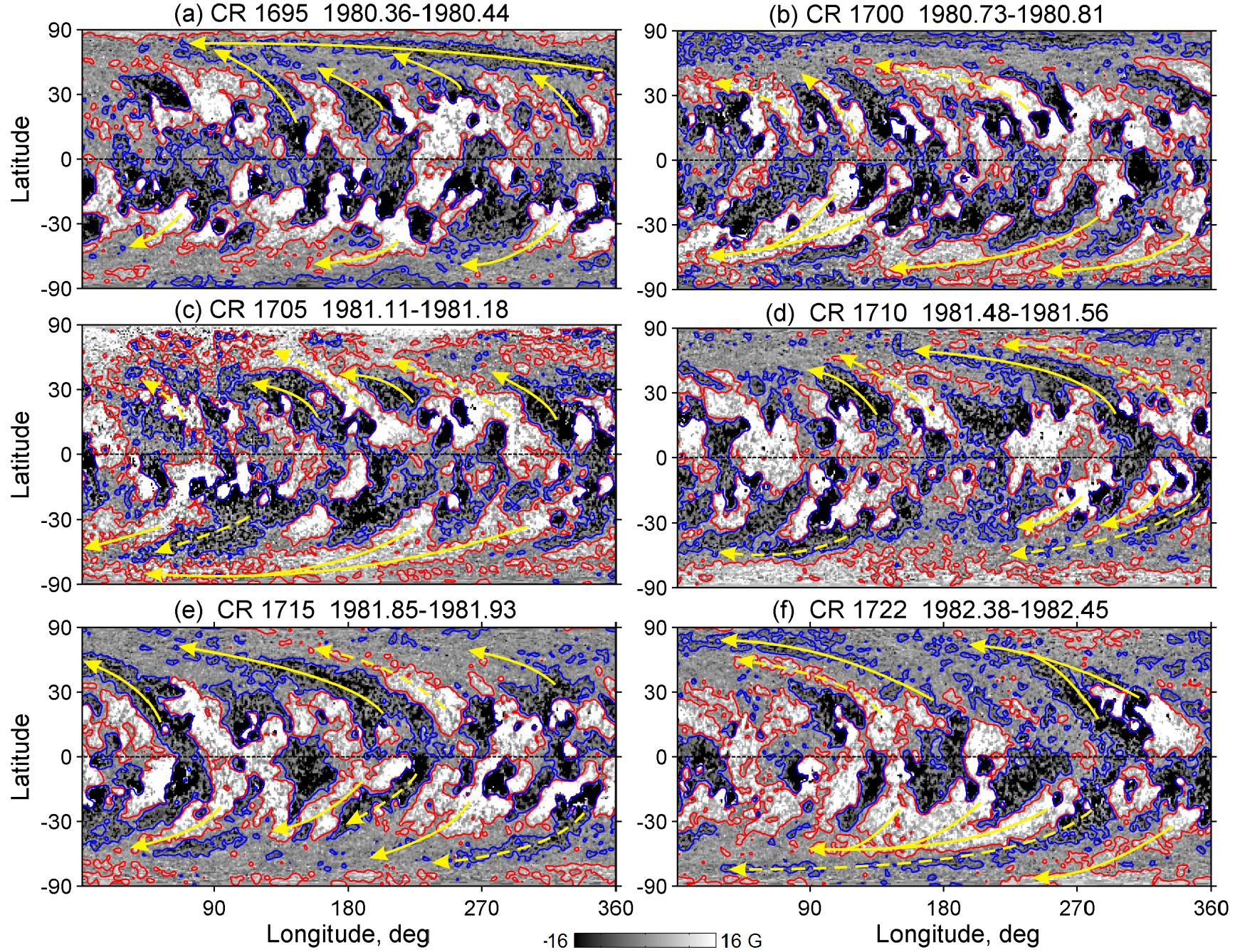
Figure 1: Synoptic maps of magnetic flux for different CRs. Positive and negative polarity UMRs are shown in white-to-black. The red and blue contours show the boundaries of UMRs corresponding to $\pm 3$ G. The trailing/leading-polarity surges are marked with solid/dashed arrows.

3 Results

3.1 A complicated restructuring of solar magnetic field in Cycle 21

Figure 1 shows original synoptic maps of magnetic flux from NSO/KPVT in black-to-white colors during the period of polar field reversals in Cycle 21. Before the reversal, positive/negative polarities dominated at the north/south poles (Figure 1a). However, at mid-latitudes in the northern hemisphere, surges of negative (trailing) polarity were formed. At latitudes above $60\degr$, trailing-polarity surges merged in a ring-shaped UMR of negative polarity. These surges originated after the decay of ARs. Then in Carrington Rotation (CR) 1700, northern hemisphere, high-latitude magnetic fields were restructured due to their poleward transport (Figure 1b). By that time at mid-latitudes, the leading-polarity (positive) surges strengthened (dashed arrows). These surges formed a tier of the leading-polarity surges, possibly which resulted in change in the dominant polarity by CR 1705 (Figure 1c). We note that the daily magnetograms have regular gaps in the Sun’s polar zones due their poor visibility. To estimate the missing data, the Kitt Peak magnetograms and all other data were filled using the extrapolation technique (Svalgaard et al., 1978b; Sun et al., 2011). Such uncertainties sometimes result in serious errors in polar zones (Bertello et al., 2014) and thus the data around polar zones should be taken with caution.

The decay of large activity complexes (ACs) in 1981–1982, led to formation of trailing-polarity surges at low- to mid-latitudes. As the cycle progressed, the trailing polarity surges approached the northern polar zone by CR 1710 (solid arrows in Figure 1d). Further strengthening of the trailing-polarity surges and their poleward transport resulted in the third change in dominant polarity at the northern polar zone (Figure 1e,f).

We note that this peculiar behavior of the polar field in the northern hemisphere and its link with the low latitude surges are highlighted by Cameron et al. (2013) in examples of equatorial flux, in particular the situation around 1980. Using the surface flux transport model, they demonstrated that a single cross-equatorial flux plumes can affect the net hemispheric flux of the following minimum by up to $60\%$. However, the observational analyses by Petrie & Ettinger (2017) show that large, long-lived complexes are the major cause of polar field change.

In the southern hemisphere, surges of trailing- and leading-polarities were also formed. By CR 1700, the trailing-polarity surges covered a wide longitude interval. Their further strengthening and the poleward transport resulted in the polar field reversal at the south pole by CR 1705. After the decay of several ARs, extensive leading-polarity surges were formed by CR 1710. During their further evolution, these surges approached south pole. However, their flux was weak to change the dominant polarity there.

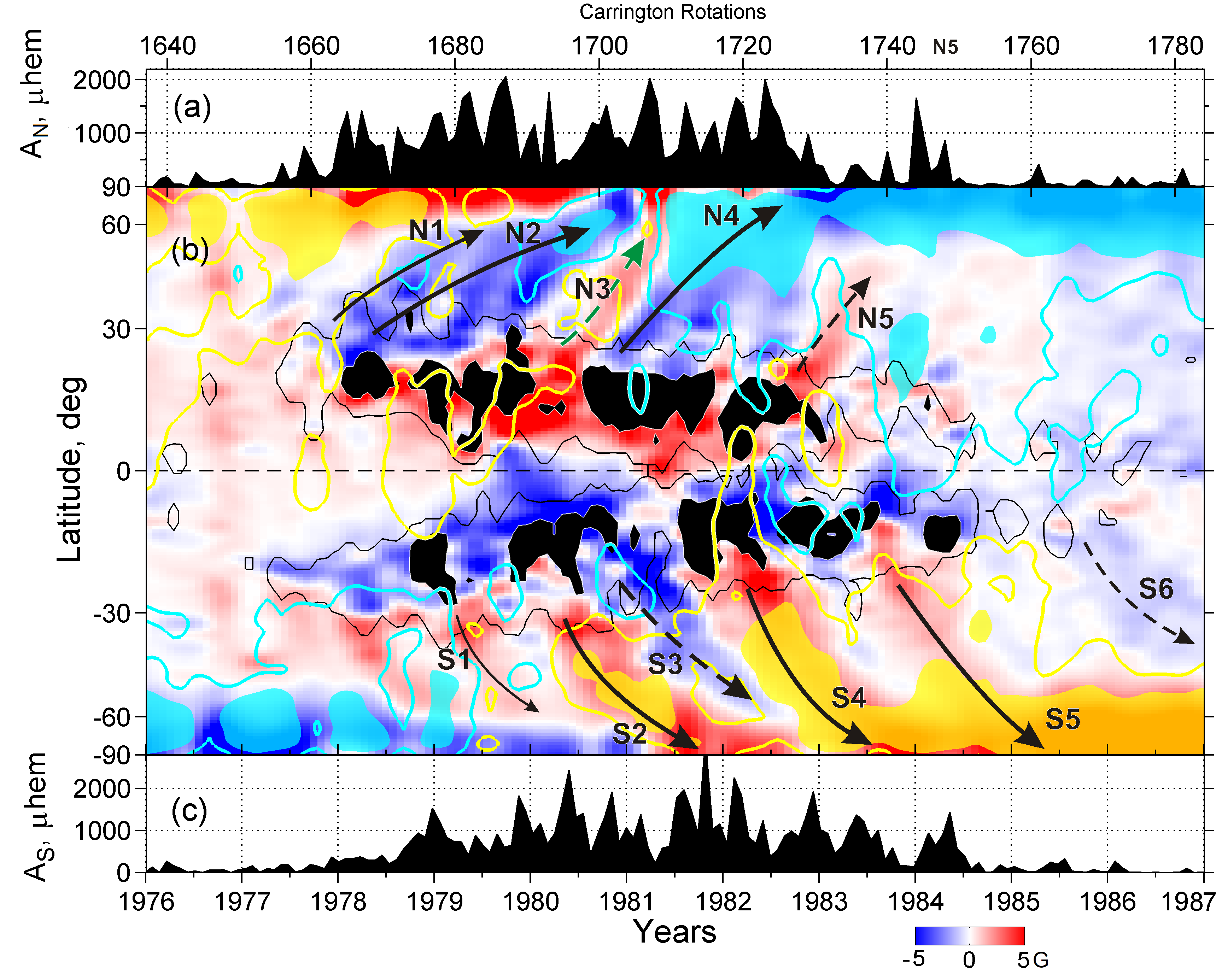
Figure 2: (a/c) Changes in sunspot areas in north/south. (b) Time-latitude variation of zonally averaged magnetic fields in the blue-to-red. Domains of high zonal flux density are shown with black spots and contours. Solid/dashed arrows show the trailing/leading-polarity surges. Domains of frequent CH appearances are shown in yellow/cyan color (at levels of $>0.1/<-0.1$). Yellow/cyan contours correspond to CH appearances at levels $\pm 0.02$.

The global reorganization of solar magnetic fields are completed by the formation of stable polar coronal holes (PCHs). As the first remnant-flux of new polarity reaches the polar zones, PCHs of the preceding cycle disappear. After the polar field reversal, new PCHs are formed due to the merger of high-latitude CHs (Golubeva & Mordvinov, 2017). The polar field buildup in every new cycle occurred in parallel with new PCH formation. Therefore, the analysis of high-latitude CHs provides independent information on the spatiotemporal behavior of polar magnetic fields.

In Figure 2b, stable polar CHs are shown by yellow/cyan spots within UMRs of positive/negative polarities. This distribution demonstrates a macro-structure of the CH ensemble. As long-lived ACs evolve and decay, their remnant magnetic fields dissipate and form UMRs.

It is believed that as the cycle progresses, the following- and leading-polarities UMRs are linked via coronal magnetic arcades (Petrie & Haislmaier, 2013). At high latitudes, however, magnetic fields tend to open up and locally unbalanced flux patterns arise. High-latitude CHs usually appear within the corridors where the magnetic field opens (Figure 2b, cyan, yellow). The arrows N2, N4, and S2, S4, S5 indicate trajectories along which magnetic flux transformations occur. Indeed, domains of emergent magnetic flux appear near the base of the arrows. Stable CHs originate at mid- to high-latitudes (near the arrow ends). The leading-polarity surges N3 and S3 disturb the regular magnetic flux transport. Small CHs appeared also within the leading-polarity surges. Thus, the CHs originated independently within the opposite polarity surges. This circumstance confirms a complicated nature of the polar fields reversal in Cycle 21. Generally, high-speed solar wind streams represent the final stage of magnetic flux evolution and its exit into the heliosphere.

3.2 Spatiotemporal Evolution of the Sun’s Magnetic Field in Cycles 21–24

In this subsection, we present the time-latitude analysis of synoptic maps averaged over longitude for CRs 1625–2241 to study a spatiotemporal evolution of Sun’s magnetic field in Cycles 21–24. We subtracted mean magnetic flux for every synoptic map. The time-latitude distribution was denoised using wavelet-based technique that recognizes domains of possible errors caused by the polar-field extrapolation. We applied Multilevel 2-D Non-Decimated Wavelet Reconstruction with Haar wavelet and level of 4. The main idea of this method is that the original time-latitude distribution is decomposed into ‘approximation’ and ‘details’ (Starck & Murtagh, 2006). The approximation shows the evolution of large-scale magnetic fields (Figure 3b). We have also examined the details which demonstrate the small-scale magnetic fields and possible defects of the time-latitude distribution due to the polar-field extrapolation. During 1977–1999, these details were concentrated in the AR areas and near the poles, more or less regularly. In Figure 3b only the details with magnetic flux density of 2 G near the poles are displayed by yellow contours. Near north pole, small-scale details usually occurred in the first half of every year. This is because the annually-varying angle between the solar rotation axis and our line of sight from (near) Earth causes the north/south pole to become unobservable during the first/second half of each year.

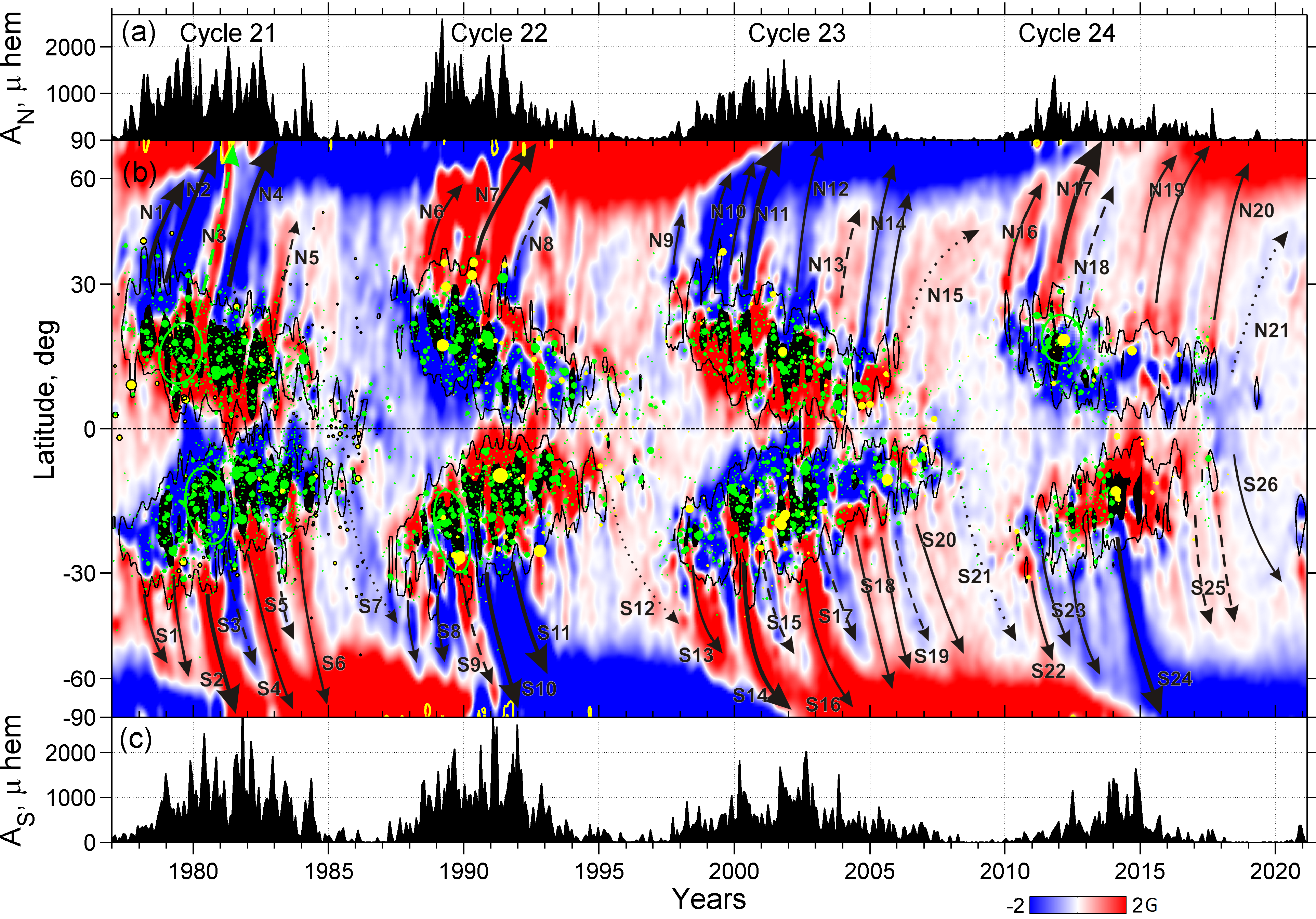
Figure 3: (a/c) Same as Figure 2. (b): Zonally averaged magnetic fields are shown in blue-to-red. Zones of intense sunspot activity are shown with black spots. Black contours depict the boundaries of sunspot activity. Solid/dashed arrows show the trailing/leading-polarity surges within the cycles, while dotted arrows show the leading-polarity surges between adjacent cycles. Non-Joy and anti-Hale ARs are marked with green/yellow markers whose diameter is proportional to sunspot areas. Yellow contours near poles show the ‘details’ of the decomposition with magnetic flux density 2 G; see §3.2 for details.

3.2.1 Cycle 21

Now, we consider Cycle 21 in a time-latitude aspect. After the decay of first ARs, the remnant flux surges N1/S1 were formed in the north/south (Figure 3b). These surges approached $\pm 60\degr$ latitudes. Reconnection of opposite magnetic polarities led to their partial annihilation, the latitudinal extent of the polar UMRs decreased. In 1978–1979, large ACs occurred in both hemispheres (Figure 3a,c). During ARs evolution and decay, weak magnetic fields were dispersed in the surrounding photosphere, forming UMRs. After the decay of long-lived ACs, a surge of negative (trailing) polarity N2 was formed in the northern hemisphere. It is marked with a solid arrow. The poleward transport of the negative-polarity UMR changed the dominant polarity (+/$-$) in late 1980. Subsequently, a surge of positive (leading) polarity (N3, green arrow) produced at low-latitudes and moved to high latitudes in 1981. The low-latitude base of surge N3 is related to non-Joy ARs that were concentrated at latitudes 5–20$\degr$ in 1979. The event N3, however, occurred during the period of poor visibility of the north pole. Under such unusual conditions, the extrapolation led to significant errors, which manifested themselves in subpolar fields during 1981. Therefore, the north pole did not necessarily reverse around this time and the pole filling technique might have imposed the sub-polar polarity reversals onto the polar fields in error.

Large ARs were observed in 1980–1981. Their decay led to the formation of a negative polarity (N4) surge, which reached the north pole and strengthened the polar cap of negative polarity. This complicated restructuring is also seen in the polar cap field of Figure 4; also see Janardhan et al. (2018). The changes in polar fields originated due to the remnant flux surges N2, N3, N4 are shown in the green rectangle in Figure 4. After the decay of anomalous ARs, UMRs of leading polarity were formed at higher latitudes. Starting from higher latitudes, these UMRs were transported poleward and resulted in the polar field reversal. The analysis of the present high-resolution synoptic maps essentially shows similar features based on the WSO data as reported in Mordvinov & Kitchatinov (2019). The timings of the reversals of the dominant polarity are listed in Table 2. As the data quality is not adequate to correctly determine the multiple reversals (if any) in the north pole for Cycle 21, we include the most likely one in Table 2.

In the southern hemisphere, a surge of the trailing (positive) polarity formed at the beginning of the cycle. The critical surge (S2) reached the south pole and led to a change in the dominant polarity ($-$/+). Later, a surge of the leading (negative) polarity (S3) was formed. It approached the south pole, but there was no change in the dominant polarity (also see Figure 4). A few abnormal ARs were observed at the base of this surge.

During 1982–1984, the decay of ARs led to the formation of intense surges S4 and S6, which restored and strengthened the magnetic field of positive polarity at the south pole. The latitudinal extent of the polar cap increased. There were many anomalous ARs in Cycle 21 (Wang & Sheeley, 1989). Their decay led to the formation of leading-polarity surges N3, N5, S3, and S5. The high level of magnetic activity and much of anomalous ARs resulted in the complicated restructuring of the subpolar flux.

The surge S7 is of particular interest. It originated from leading-polarity UMR at the end of Cycle 21. Its path indicates the magnetic flux transport from Cycle 21 and merged with new magnetic flux of the same polarity in the next cycle. This merger leads to an increase in the magnetic field in a new cycle and early reversal in south (also see Figure 4). This phenomenon indicates that not all of the magnetic flux disappears by the end of the old cycle; part of it can be transferred from one cycle to the next and amplify the field.

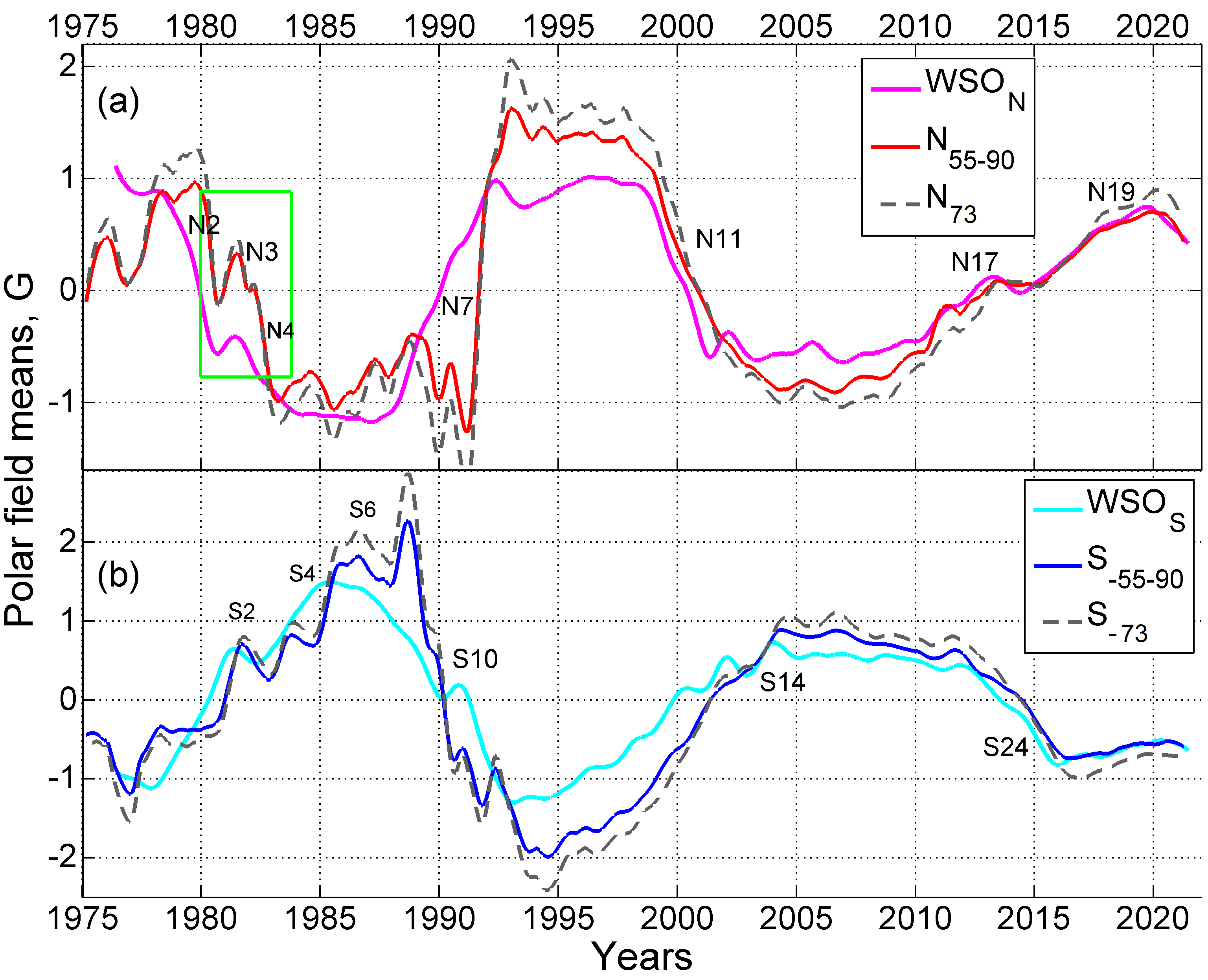
Figure 4: Magenta/cyan: north/south polar fields from the daily line-of-sight measurements with 20 nHz low pass filtered at WSO. Red/blue: north/south polar-cap magnetic flux densities computed by averaging of magnetic fields at latitudes since $\pm 55^{\circ}$ to pole in the radial synoptic maps. Gray dashed lines show the mean flux densities at latitudes $\pm 73^{\circ}$ in the maps. Here, for ease of comparison, the synoptic map data are converted to the WSO scale using the conversion factors (Riley et al., 2014).

3.2.2 Cycle 22

In Cycle 22, after the decay of the first ARs, trailing-polarity surges N6 and S8 were formed (Figure 3b). These surges annihilated at about $\pm 60^{\circ}$ latitudes, and thereby reduced the polar magnetic flux. During 1989–1992, plenty of sunspots appeared. The critical surges N7 and S10 reached the poles and changed the dominant polarity. In the southern hemisphere, there were intense surges S10, S11 which represent cumulative effects of two activity impulses (Figure 3c). In both hemispheres, regular polar field reversals occurred. Such an evolution of magnetic field is quite consistent with the Babcock–Leighton scenario.

Nevertheless, these patterns were disrupted by leading-polarity surges. In both hemispheres well-defined surges N8 and S9 of leading polarity occurred. At the base of these surges, abnormal ARs were observed. The leading-polarity surge S9 was not strong enough to cause a clear dip in the polar-cap field in Figure 4 around 1991. Afterward around 1992 in Figure 4, there was a clear depression in the south polar-cap field, the signature of which is not visible in the time-latitude plot. This depression in the polar-cap field caused a double peak in the following sunspot Cycle 23 of the southern hemisphere. This connection between the polar field depression and the double peak was demonstrated in Karak et al. (2018) based on the observations and dynamo model. As there is no prominent drop in the polar field in the northern hemisphere, no double peak seen in the same hemisphere for Cycle 23.

Again, in the southern hemisphere of Cycle 22, we find a link between adjacent cycles. After the decay of the last ARs, a surge of (positive) leading-polarity S12 was formed and transported in mid-latitudes until it merged with S13, which had the same polarity as that in Cycle 23.

3.2.3 Cycle 23

In 1997, the decay of first ARs appeared around $\pm 30\degr$ latitudes form UMRs of both polarities (Figure 3b). Trailing polarity UMR N9 is well-defined. The decay of subsequent ARs was associated with surges N10 that reached higher latitudes. The decay of long-lived ARs in 2000 led to the formation of the critical surge N11, which reached the north pole and led to a change in the dominant polarity (+/$-$). Subsequent bursts of activity were associated with surges N12, N14, that strengthened magnetic flux at the north pole. The leading-polarity surge N13 is apparently associated with non-Joy ARs at low latitudes.

At the end of Cycle 23, the leading-polarity UMRs dominated near the equator. During the activity minimum, the meridional flow led to formation of an extended surge of the remnant flux N15, which reached latitudes of $40-60\degr$ by the beginning of Cycle 24. Subsequently, a surge N16 of a new cycle was formed at low latitudes. The merger of the positive polarity UMRs led to an increase in the net remnant flux of the new cycle. Thus, again the transport of magnetic flux between adjacent cycles reveals a new mechanism that links individual cycles into pairs.

In south, a complex structure of remnant flux was observed. In 2000, decay of great ARs generates critical surge S14. Subsequent trailing-polarity surges S16, S18, and S20 strengthened the magnetic flux in the polar region. The leading-polarity surges S15, S17, and S19 tried to reduce the polar flux. Surge S17 clearly caused a little depression in the polar-cap field as seen in Figure 4. At the end of Cycle 23, leading-polarity surge S21 was formed.

We finally notice that as there is no prominent depression in the north/south polar field in Cycle 23 (Figure 4), there are no pronounced double peaks in the following cycle.

3.2.4 Cycle 24

This is the most important cycle because the magnetic activity was low, and this field is the precursor for the upcoming Cycle 25. The north-south asymmetry of the Sun’s activity has led to a significant asynchronous reversal of the polar fields. At the beginning of the cycle, magnetic activity prevailed in the northern hemisphere. During the decay of the first ARs in the northern hemisphere, surge N16 was formed (Figure 3b). The critical surge N17 reached the north pole and changed the dominant polarity ($-$/+) in early 2013.

During 2012–2013, the activity was low and a leading-polarity surge N18 was formed. During that time, anomalous ARs were observed at low latitudes. As surge N18 approached the north pole, magnetic flux decreased to almost zero due to annihilation of opposite polarities (also see Figure 4). The decay of ARs in 2014–2017 resulted in surges N19, N20. The poleward transport of remnant flux led to significant strengthening of the polar field in the north pole. At the end of the cycle, the leading-polarity surge N21 was formed. This surge reached mid-latitudes by 2021. It already corresponds to upcoming Cycle 25.

At the beginning of cycle in southern hemisphere, decay of anti-Hale and non-Joy ARs led to the formation of a leading-polarity surge S22. Its poleward transport overpowers the previous polarity polar field and destroys the weak surge S21 from the previous cycle. Further appearance of ARs and their decay led to the formation of trailing-polarity surges S23. The emergent magnetic flux peaked in 2014 for south. After the decay of largest ARs in 2014, a critical surge S24 was formed. This surge reached the south pole and changed the dominant polarity by mid-2015 (+/$-$). During the decline phase of activity, leading-polarity surges S25 were formed. Finally, surge S26 originated from the transequatorial UMR in the southern hemisphere.

Table 2: Changes in the dominant magnetic fields in the subpolar zones for Cycles 21–24.

Cycle number	21	22	23	24
North pole	1982.5	1991.7	2001.8	2013.3
South pole	1981.1	1990.2	2001.9	2015.4

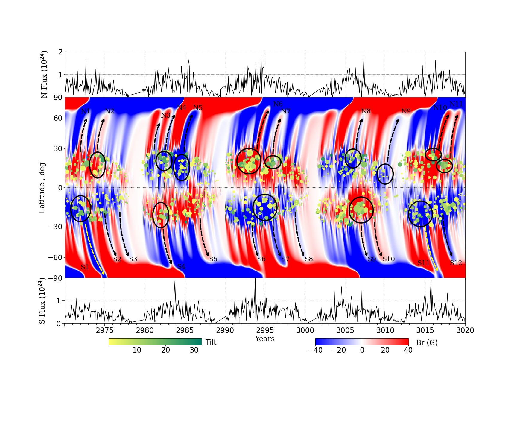
Figure 5: Results from dynamo model: The butterfly diagram of the radial magnetic field in Gauss (middle). Filled points represent anti-Hale BMRs with tilt deviating from Joy’s law by more than $50\%$. The colorbar shows the modulus of the tilt. The size of the points indicates the amount of flux, while color shows the amount of absolute tilt (in degree); see left colorbar. Top and bottom panels show the variations of the monthly magnetic fluxes of BMRs in the northern and southern hemispheres in Mx.

4 Leading polarity surges and a triple reversal in a Babcock–Leighton dynamo model

Here we present a snapshot of the surface radial magnetic field from a dynamo model to explore and compare the results with the observational ones. Our result is obtained from Run B1 which was presented in Karak (2020) and it is based on the 3D dynamo model, STABLE (Miesch & Dikpati, 2014; Miesch & Teweldebirhan, 2016; Karak & Miesch, 2017). The details of the model which produces our result are described in Karak (2020). Therefore, without writing the mathematical details of the model, we mention here the salient features. Essentially, in this model, we solve the kinematic dynamo equation by specifying single-cell meridional flow, differential rotation, turbulent diffusivity, and magnetic pumping, all consistent with the available solar observations (Karak & Cameron, 2016). The model includes a sophisticated procedure for the BMR eruptions on the surface, based on the toroidal field at the tachocline. The eruption is possible only when the time delay between the eruptions exceeds a certain delay $\Delta$ and the mean azimuthal field in the tachocline exceeds a certain threshold value $B_{t}$. The $\Delta$ is obtained from a log-normal distribution which is fixed in this simulation. While $B_{t}=2$ kG at the equator, it increases exponentially with the latitude. This helps to restrict BMRs in low- to mid-latitudes and importantly, the observed cycle-dependent latitude distribution of BMR, namely the stronger cycle (on average) produces BMRs at higher latitudes than the weaker ones. The latter feature is sufficient to produce a nonlinearity to halt the growth of the dynamo (Karak, 2020). Statistical features of BMRs are obtained from observations, particularly the tilt is obtained from Joy’s law with a Gaussian scatter around it having $\mu=0$ and $\sigma=15\degr$ (Stenflo & Kosovichev, 2012; Jha et al., 2020).

In Figure 5, we present the surface radial field as a function of time and latitude. One discrepancy in this model is that the strength of the radial field is much stronger than that is observed in the Sun. Despite this, we observe the basic features of the solar cycle, including, polarity reversal, pole-ward migration and hemispheric asymmetry. We also observe a lot of details of the magnetic field at small scales which are in good agreement with the observation. The leading polarity surges which are originated at low- to mid-latitudes, migrate, and merge with the global field near the pole. Some of these leading polarity surges are so strong that they disturb the polar field significantly. Karak & Miesch (2017); Hazra et al. (2017); Karak & Miesch (2018) showed that the anti-Hale spots are responsible for changing the polar field and consequently the next cycle strength in this dynamo model. The anti-Hale BMRs having tilt deviation more than $50\%$ from Joy’s law are shown by color points in Figure 5. We observe some connection (although it is not always obvious in this plot) between the domains of highly tilted BMRs with large flux contents and the leading polarity surges, as marked by dashed arrows. As the time delay between two BMRs is not fixed and it is taken from an observed distribution, the rate of BMR eruption is not constant. This leads to some variation in the magnetic field. In this figure, we find clear evidence of a triple reversal in the southern polar field around the year 2975, which is caused by a strong leading polarity surge S1 (yellow dashed arrow) that originated around $15\degr$ latitude. Therefore, although the triple reversal in the Sun is not conclusively known due to the defects in the data of the polar regions, it may be possible in the Sun as supported by a Babcock–Leighton dynamo model. The surge S6 that appeared around the year 3016 in the southern hemisphere is very interesting. It enhanced the old polarity (negative) field and caused a delay in the reversal of the pole. Had this surge appeared after a few months, this could lead to another triple reversal of the south pole. We note that the triple reversal in the dynamo model is very rare. In our simulation of around 500 years, we find one clear triple reversal which is shown in Figure 5. In future work, we shall present a detailed analysis of the statics of triple reveals in this dynamo model, by running the model for several thousands of years in different parameters.

5 Summary and Conclusions

We analyzed the high-resolution synoptic magnetic maps for Cycles 21–24. We identify major remnant flux surges and their sources, reexamine the polar field buildup and reversals in their causal relation to the Sun’s low-latitude activity. A spatiotemporal behavior of the Sun’s magnetic flux depicts a general evolution of the Sun’s magnetic field and its effect on PCHs.

The time-latitude analysis of AR tilts showed that surges of leading polarity appeared after the decay of non-Joy and anti-Hale ARs. When such an AR is highly tilted and appears near the equator, it produces a strong leading polarity surge which can disturb a dominant polarity flux considerably (Cameron et al., 2013; Karak & Miesch, 2017; Nagy et al., 2017). We also found inter-cyclic remnant flux surges between adjacent 11-year cycles. These surges reveal the physical links between subsequent solar cycles. The individual 11-year cycles are linked in pairs. This interrelation between 11-year cycles suggests a possible long-term memory in solar activity that manifests itself on a secular timescale.

Preliminary analyses of the magnetic field from a 3D Babcock–Leighton dynamo model demonstrate some support for the generation of leading-polarity surges at low-latitudes, their transport towards poles and changes in the dominant polarity field. The model also shows a clear evidence of triple reversal, although it is very rare. Therefore, although the triple reversal in the Sun is not very conclusive due to the known defects in the data of the polar regions, such phenomenon is not fundamentally impossible from the point of view of the Babcock–Leighton dynamo model.

DATA AVAILABILITY

NSO/Kitt Peak data used here are produced cooperatively by NSF/NOAO, NASA/GSFC, NOAA/SEL, and Bartol. Data were acquired by SOLIS instruments operated by NISP/NSO/AURA/NSF. SOHO is a project of international cooperation between ESA and NASA. The SDO/HMI data are available by courtesy of NASA/SDO and the AIA, EVE, and HMI science teams. ”Bipolar magnetic regions determined from KPVT full disk magnetograms” were downloaded from the solar dynamo dataverse (https://dataverse.harvard.edu/dataverse/solardynamo), maintained by Andrés Muñoz-Jaramillo. Data and the routines of our analyses presented in the article will be shared upon reasonable request to the corresponding author. Wilcox Solar Observatory data used in this study was obtained via the web site http://wso.stanford.edu courtesy of J.T. Hoeksema. The Wilcox Solar Observatory is currently supported by NASA.

References

- Babcock (1961) Babcock H. W., 1961, ApJ, 133, 572
- Babcock & Babcock (1955) Babcock H. W., Babcock H. D., 1955, ApJ, 121, 349