IFT-UAM/CSIC-21-116
December 17^th, 2021

We study extremal 5- and 4-dimensional black hole solutions of the Heterotic Superstring effective action at first order in $\alpha^{\prime}$ with, respectively, 3 and 4 charges of arbitrary signs. For a particular choice of the relative signs of these charges the solutions are supersymmetric, but other signs give rise to non-supersymmetric extremal black holes. Although at zeroth order all these solutions are formally identical, we show that the $\alpha^{\prime}$ corrections are drastically different depending on how we break supersymmetry. We provide fully analytic $\mathcal{O}(\alpha^{\prime})$ solutions and we compute their charges, masses and entropies and check that they are invariant under $\alpha^{\prime}$-corrected T-duality transformations. The masses of some of these black holes are corrected in a complicated way, but we show that the shift is always negative, in agreement with the Weak Gravity Conjecture. Our formula for the corrected entropy of the four-dimensional black holes generalizes previous results obtained from the entropy function method, as we consider a more general way in which supersymmetry can be broken.

1 Introduction

Black holes provide an excellent ground for testing string theory as a quantum theory of gravity. The statistical derivation of the Bekenstein-Hawking entropy of 5-dimensional supersymmetric black holes by Strominger and Vafa [1] remains, to this day, one of the main tests passed by string theory in this direction. Since then, a great deal of work has been devoted to push this comparison beyond leading order in the large-charge expansion. On the microscopic side, this implies that one has to compute corrections to Cardy’s formula [2, 3]. On the gravitational side, instead, one has to take into account $\alpha^{\prime}$ corrections to supergravity, which encode genuine stringy effects. For this comparison to be possible and meaningful, several things are needed from the gravitational side:

1. Knowledge of the string effective action to higher order in $\alpha^{\prime}$.

2. Black-hole solutions of the higher-order equations derived from those actions.

3. A consistent procedure to compute the analog of the Bekenstein-Hawking entropy in higher-order theories.

4. A dictionary relating the parameters of the black-hole solutions (mass, angular momenta, charges, moduli) to those of the microscopic system.

Let us comment upon each of these points.

1. Our knowledge of the higher-order in $\alpha^{\prime}$ corrections to the string effective action is very incomplete as they are only known for the first few orders. Among the supersymmetric string theories, only the heterotic has first-order corrections and these and the second- and third-order ones are also known [4, 5, 6, 7]. This makes this theory especially well-suited for the the computation of $\alpha^{\prime}$ corrections to black-hole solutions. Since the complexity of the calculations increases rapidly with the power of $\alpha^{\prime}$, only the first-order ones have typically been computed.

2. Only a few analytic stringy black hole solutions are known to first order in $\alpha^{\prime}$ [8, 9, 10, 11, 12, 13, 14]. Many results on $\alpha^{\prime}$ corrections to black-hole entropies are based on the entropy function formalism [15]. Its main advantage is that only deals with the near-horizon geometries, circumventing the task of solving the corrected equations of motion. It has however some limitations because one loses information about the asymptotic region, and, for instance, one cannot get the mass of the black holes. Also, the interpretation of the charges is arguably less transparent in this formalism.

   One of the main goals of this paper is to increase the number of complete first-order in $\alpha^{\prime}$ black hole solutions known by determining the first-order $\alpha^{\prime}$ corrections to all the most basic 3-charge, 5-dimensional and 4-charge, 4-dimensional extremal black holes. This implies allowing for all the possible signs of the charges. Only some combinations of the signs of the charges are compatible with supersymmetry, as it is well known [16]. Some non-supersymmetric choices have been considered in the literature [2, 17, 18] but, here, we consider all of them and, as we are going to see, the $\alpha^{\prime}$ corrections to the solutions turn out to be wildly different for different sign choices.

   Besides, these solutions are interesting to test the so-called mild form of the Weak Gravity Conjecture [19, 20, 21], according to which, the corrections to the mass of extremal black holes should be negative in a consistent theory of quantum gravity. This conjecture has been applied in a number of scenarios to constrain the parameters of effective field theories [22, 23, 24, 25, 26, 27, 28, 29, 30, 31]. However, by studying the effect of higher-derivative corrections coming explicitly from string theory, one can in turn test this conjecture [32, 13], as in that case it is expected to be satisfied.

3. Using the formalism developed in Ref. [33], Wald showed that, in a diffeomorphism-invariant theory of gravity, the black-hole entropy can be identified with the Noether charge associated to diffeomorphisms evaluated for the Killing vector normal on the event horizon, because this is the quantity whose variation appears multiplied by the temperature in the first law of black-hole mechanics [34]. This entropy (Wald entropy) coincides with the Bekenstein-Hawking entropy for General Relativity but can also be used in theories of higher order in the curvature such as the higher order in $\alpha^{\prime}$ string effective action. However, this action also contains matter fields, which were not considered in Ref. [34].

   In Ref. [35] Iyer and Wald considered matter fields, assuming they behave as tensors under diffeomorphisms and gave a recipe for computing the Wald entropy (the Iyer-Wald entropy formula) which has become standard in the literature. However, as discussed in more detail in Refs. [36, 37, 38], the only field in the Standard Model that transforms as a tensor is the metric. The rest have gauge freedoms and their transformations under diffeomorphisms always involve “compensating gauge transformations” that have to be properly taken into account. Only then one obtains the work terms in the first law of black-hole mechanics which, actually, were not derived in Ref. [35]. These terms arise from additional contributions to the diffeomorphisms Noether charge, which means that, in general, the entropy is not the Noether charge and the derivation of the first law with all the terms that contribute to it is a conditio sine qua non for the identification of the Wald entropy.

   In Ref. [38] a gauge-invariant entropy formula for the Heterotic Superstring effective action at first order in $\alpha^{\prime}$ was derived after taking into account all the complicated gauge transformations of the theory. This formula gives unambiguous results and, in the few examples in which the entropy has been computed by other methods, it gives the same result.

   The second main goal of this paper is to compute the entropy of the $\alpha^{\prime}$-corrected solutions we are going to find using this formula.

4. Finding a stringy interpretation of the parameters occurring in the simplest leading-order black-hole solutions presents no special problems because, first of all, the Chern-Simons terms that occur in the 4- and 5-dimensional field strengths vanish and all the definitions of conserved charge (Page, Maxwell) give the same result. Furthermore, the potentials that occur in the effective action have a clear stringy interpretation. One can, then, express the charges in terms of the numbers of certain branes defining the background in which the string is quantized. These numbers occur in the resulting CFT whose states are counted and in the microscopic entropy. The comparison with the macroscopic one is, therefore, straightforward.

   When the $\alpha^{\prime}$ corrections are switched on, though, the Chern-Simons terms in the field strengths become active and, on top of this, higher-derivative terms are added to the equations of motion of the potentials. The values of the conserved charges are then different for different definitions and their physical interpretation in terms of branes is far less clear. We believe this is a problem to which insufficient attention has been paid so far and which is crucial for having a convincing comparison of macroscopic and microscopic computations of black-hole entropies. We will investigate it in more depth elsewhere [42] and, here, we will content ourselves with using simple and intuitive notions of charge.

This paper is organized as follows: in Section 2 we review the Heterotic Superstring effective action (equations of motion and supersymmetry transformations) to first order in $\alpha^{\prime}$ in the Bergshoeff-de Roo formulation [7]. In Section 3 we focus on the 5-dimensional, static, 3-charge, extremal black hole solutions of the theory, originally studied in Refs. [43, 44, 45]. First of all, in Section 3.1, we present a 10-dimensional ansatz the encompasses all the solutions that we are going to study. In Section 3.2 we study the unbroken supersymmetries of the ansatz for different signs of the three charges and the 5-dimensional form of the ansatz obtained by compactification on a T⁵ in Section 3.3. The $\alpha^{\prime}$ corrections are presented in Section 3.4 and the calculation of their Wald entropies is carried out in Section 3.5.

In Section 4 we focus on 4-dimensional, static, 4-charge, extremal black hole solutions of the theory, which includes the heterotic version of the black holes studied in Refs. [46, 47, 48]. Again, we start by presenting in Section 4.1 a general ansatz that encompasses all the solutions that we are going to consider, in Section 4.2 we study its unbroken supersymmetry for different signs of the charges and in Section 4.3 we give the 4-dimensional form of the ansatz, obtained by compactification on a T⁶. In Section 4.4 we present the $\alpha^{\prime}$ corrections, which now depend very strongly on the relative signs of the charges. We write the fields of the $\alpha^{\prime}$-corrected solutions in a manifestly T duality-invariant form. In Section 4.5 we present the computation of the Wald entropy of the $\alpha^{\prime}$-corrected solutions.

In Section 5 we explore the use of $\alpha^{\prime}$-corrected T duality to help us determine the form of the $\alpha^{\prime}$ corrections to the solutions in the 5- and 4-dimensional cases considered here. Finally, in Section 6 we discuss different aspects of the solutions presented in this paper.

2 The Heterotic Superstring effective action

For the sake of self-consistency, we are going to give a short description of the Heterotic Superstring (HST) effective action and the fermionic supersymmetry transformation rules to first order in $\alpha^{\prime}$ as given in [7] using the conventions of Ref. [49]. We remind the reader that $\alpha^{\prime}=\ell_{s}^{2}$, where $\ell_{s}$ is the string length.

The HST effective action describes the massless degrees of freedom of the HST: the (string-frame) Zehnbein $e^{a}=e^{a}{}_{\mu}dx^{\mu}$, the Kalb-Ramond 2-form $B=\tfrac{1}{2}B_{\mu\nu}dx^{\mu}\wedge dx^{\nu}$, the dilaton $\phi$ and the Yang-Mills field $A^{A}=A^{A}{}_{\mu}dx^{\mu}$ (where $A,B,C,\ldots$ take values in the Lie algebra of the gauge group). In certain cases we will use hats to distinguish the 10-dimensional fields from those obtained from them by dimensional reduction.

We start by defining the (torsionless, metric-compatible) Levi-Civita spin connection 1-form $\omega^{a}{}_{b}=\omega_{\mu}{}^{a}{}_{b}dx^{\mu}$, which in our conventions satisfies the Cartan structure equation in the form

$$\mathcal{D}e^{a}\equiv de^{a}-\omega^{a}{}_{b}\wedge e^{b}=0\,.$$ (2.1)

The theory is, however, most conveniently described in terms of a pair of torsionful spin (or Lorentz) connections ${\Omega}^{(0)}_{(\pm)}{}^{{a}}{}_{{b}}={\Omega}^{(0)}_{(\pm)\,\mu}{}^{{a}}{}_{{b}}dx^{\mu}$ obtained by adding an extra term to the Levi-Civita connection

$${\Omega}^{(0)}_{(\pm)}{}^{{a}}{}_{{b}}={\omega}^{{a}}{}_{{b}}\pm\tfrac{1}{2}{H}^{(0)}_{{\mu}}{}^{{a}}{}_{{b}}dx^{{\mu}}\,.$$ (2.2)

In this definition, $H^{(0)}_{{\mu}}{}^{{a}}{}_{{b}}$ are the components of the zeroth order Kalb-Ramond 3-form field strength

$$H^{(0)}\equiv dB\,.$$ (2.3)

The curvature 2-forms of these connections and the (Lorentz-) Chern-Simons 3-forms are defined as

$${R}^{(0)}_{(\pm)}{}^{{a}}{}_{{b}} = d{\Omega}^{(0)}_{(\pm)}{}^{{a}}{}_{{b}}-{\Omega}^{(0)}_{(\pm)}{}^{{a}}{}_{{c}}\wedge{\Omega}^{(0)}_{(\pm)}{}^{{c}}{}_{{b}}\,,$$ (2.4)

$${\omega}^{{\rm L}\,(0)}_{(\pm)} = d{\Omega}^{(0)}_{(\pm)}{}^{{a}}{}_{{b}}\wedge{\Omega}^{(0)}_{(\pm)}{}^{{b}}{}_{{a}}-\tfrac{2}{3}{\Omega}^{(0)}_{(\pm)}{}^{{a}}{}_{{b}}\wedge{\Omega}^{(0)}_{(\pm)}{}^{{b}}{}_{{c}}\wedge{\Omega}^{(0)}_{(\pm)}{}^{{c}}{}_{{a}}\,.$$ (2.5)

The curvature 2-form and Chern-Simons 3-form of the Yang-Mills field are defined, respectively, by

$${F}^{A} = d{A}^{A}+\tfrac{1}{2}f_{BC}{}^{A}{A}^{B}\wedge{A}^{C}\,,$$ (2.6)

$${\omega}^{\rm YM} = dA_{A}\wedge{A}^{A}+\tfrac{1}{3}f_{ABC}{A}^{A}\wedge{A}^{B}\wedge{A}^{C}\,.$$ (2.7)

In the last expression we have used the Killing metric of the gauge group’s Lie algebra in the relevant representation, $K_{AB}$ (which we assume to be invertible and positive definite) to lower adjoint indices $A,B,C,\ldots$.

Now we can define the first-order Kalb-Ramond 3-form field strength as

$$H^{(1)}=d{B}+\frac{\alpha^{\prime}}{4}\left({\omega}^{\rm YM}+{\omega}^{{\rm L}\,(0)}_{(-)}\right)\,.$$ (2.8)

Replacing $H^{(0)}$ by $H^{(1)}$ in the definition of the torsionful spin connections Eq. (2.2) we obtain the first-order torsionful spin connections ${\Omega}^{(1)}_{(\pm)}{}^{{a}}{}_{{b}}$ whose Chern-Simons 3-form ${\omega}^{{\rm L}\,(1)}_{(\pm)}$ can be used in Eq. (2.8) to define the second-order Kalb-Ramond 3-form field strength $H^{(2)}$ etc. In the first-order action we only need $H^{(1)}$, ${\Omega}^{(0)}_{(-)}{}^{{a}}{}_{{b}}$ and its curvature 2-form $R^{(0)}_{(-)}{}^{a}{}_{b}$ and Chern-Simons 3-form ${\omega}^{{\rm L}\,(0)}_{(-)}$. The kinetic term for $H^{(1)}$ (quadratic) will contain terms of second order in $\alpha^{\prime}$ which contribute to the equations of motion and which we should ignore. Keeping them, though, makes the action explicitly gauge invariant instead of invariant up to terms of second order in $\alpha^{\prime}$.

The explicit $\alpha^{\prime}$ corrections in the action, equations of motion and in the Bianchi identity of the Kalb-Ramond 3-form field strength can be conveniently described in terms of the so-called “$T$-tensors”, defined by

$$\begin{array}[]{rcl}{T}^{(4)}&\equiv&\dfrac{\alpha^{\prime}}{4}\left[{F}_{A}\wedge{F}^{A}+{R}_{(-)}{}^{{a}}{}_{{b}}\wedge{R}_{(-)}{}^{{b}}{}_{{a}}\right]\,,\\ &&\\ {T}^{(2)}{}_{{\mu}{\nu}}&\equiv&\dfrac{\alpha^{\prime}}{4}\left[{F}_{A}{}_{{\mu}{\rho}}{F}^{A}{}_{{\nu}}{}^{{\rho}}+{R}_{(-)\,{\mu}{\rho}}{}^{{a}}{}_{{b}}{R}_{(-)\,{\nu}}{}^{{\rho}\,{b}}{}_{{a}}\right]\,,\\ &&\\ {T}^{(0)}&\equiv&{T}^{(2)\,\mu}{}_{{\mu}}\,.\\ \end{array}$$ (2.9)

The string-frame HST effective action is, to first order in $\alpha^{\prime}$,

$$S=\frac{g_{s}^{2}}{16\pi G_{N}^{(10)}}\int d^{10}x\sqrt{|{g}|}\,e^{-2{\phi}}\,\left\{{R}-4(\partial{\phi})^{2}+\tfrac{1}{12}{H}^{(1)\,2}-\tfrac{1}{2}T^{(0)}\right\}\,,$$ (2.10)

where $R$ is the Ricci scalar of the string-frame metric $g_{\mu\nu}=\eta_{ab}e^{a}{}_{\mu}e^{b}{}_{\nu}$, $G_{N}^{(10)}$ is the 10-dimensional Newton constant , $g_{s}$ is the HST coupling constant (the vacuum expectation value of the dilaton $e^{<\phi>}$ which we will identify with the asymptotic value of the dilaton $e^{\phi_{\infty}}$ in asymptotically-flat black-hole solutions).

The 10-dimensional Newton constant depends on the string length and coupling constant in this way:

$$G_{N}^{(10)}=8\pi^{6}g_{s}^{2}\ell_{s}^{8}\,.$$ (2.11)

The naive variation of the action Eq. (2.10) leads to very complicated equations of motion which contain terms with higher derivatives, all of them coming from the variation of the torsionful spin connection in different terms. However, the lemma proven in Ref. [7] allows us to consistently ignore all those terms because they give contributions of second and higher orders in $\alpha^{\prime}$. Thus, the equations that we effectively have to solve to first order in $\alpha^{\prime}$ come from the variation of the action with respect to the explicit (i.e. not in the torsionful spin connection) occurrences of the fields. After some recombinations, they can be written in the standard form found in the literature

$$R^{\mu}{}_{a}-2\nabla^{\mu}\partial_{a}\phi+\tfrac{1}{4}{H}^{\mu\rho\sigma}{H}_{a\rho\sigma}-T^{(2)\,\mu}{}_{a} = 0\,,$$ (2.12)

$$(\partial\phi)^{2}-\tfrac{1}{2}\nabla^{2}\phi-\tfrac{1}{4\cdot 3!}{H}^{2}+\tfrac{1}{8}T^{(0)} = 0\,,$$ (2.13)

$$\nabla_{\mu}\left(e^{-2\phi}H^{\mu\nu\rho}\right) = 0\,,$$ (2.14)

$$\alpha^{\prime}e^{2\phi}\nabla_{(+)\,\mu}\left(e^{-2\phi}F^{A\,\mu\nu}\right) = 0\,.$$ (2.15)

The Einstein equation can be rewritten in a more compact form using the identity

$$R^{\mu}{}_{a}(\Omega^{(\pm)})-2\nabla^{(\pm)\,\mu}\partial_{a}\phi=R^{\mu}{}_{a}(\omega)+\tfrac{1}{4}H^{\mu bc}H_{abc}-2\nabla^{\mu}\partial_{a}\phi\pm\tfrac{1}{2}e^{2\phi}\nabla^{\nu}\left(e^{-2\phi}H^{\mu\nu}{}_{a}\right)\,,$$ (2.16)

and combining it with the Kalb-Ramond equation:

$$R^{\mu}{}_{a}(\Omega^{(\pm)})-2\nabla^{(\pm)\,\mu}\partial_{a}\phi-T^{(2)\,\mu}{}_{a}=0\,.$$ (2.17)

To first order in $\alpha^{\prime}$ and for vanishing fermions, the supersymmetry transformation rules of the gravitino $\psi_{\mu}$, dilatino $\lambda$ and gaugini $\chi^{A}$ (all of them 32-component Majorana-Weyl spinors, $\psi_{\mu},\chi^{A}$ and $\epsilon$ with positive chirality and $\lambda$ with negative chirality) are

$$\delta_{\epsilon}\psi_{a} = \nabla^{(+)}{}_{a}\,\epsilon\equiv\left(\partial_{a}-\tfrac{1}{4}\Omega^{(+)}{}_{a\,bc}\Gamma^{bc}\right)\epsilon\,,$$ (2.18)

$$\delta_{\epsilon}\lambda = \bigg{(}\partial_{a}\phi\Gamma^{a}-\tfrac{1}{12}H_{abc}\Gamma^{abc}\bigg{)}\epsilon\,,$$ (2.19)

$$\alpha^{\prime}\delta_{\epsilon}\chi^{A} = -\tfrac{1}{4}\alpha^{\prime}F^{A}{}_{ab}\Gamma^{ab}\epsilon\,.$$ (2.20)

We will not include Yang-Mills fields in our solutions.

3 3-charge, 5-dimensional black holes

3.1 10-dimensional form

The extremal 3-charge, 5-dimensional black holes we want to study were originally obtained in [43, 44, 45]. A common 10-dimensional ansatz for them is

$$d\hat{s}^{2} =\frac{1}{\mathcal{Z}_{+}\mathcal{Z}_{-}}dt^{2}-\mathcal{Z}_{0}(d\rho^{2}+\rho^{2}d\Omega_{(3)}^{2})$$

$$-\frac{k_{\infty}^{2}\mathcal{Z}_{+}}{\mathcal{Z}_{-}}\left[dz+\beta_{+}k_{\infty}^{-1}\left(\mathcal{Z}^{-1}_{+}-1\right)dt\right]^{2}-dy^{m}dy^{m}\,,\hskip 14.22636ptm=1,\ldots,4\,,$$ (3.1a)

$$\hat{H} =d\left[\beta_{-}k_{\infty}\left(\mathcal{Z}^{-1}_{-}-1\right)dt\wedge dz\right]+\beta_{0}\rho^{3}\mathcal{Z}^{\prime}_{0}\omega_{(3)}\,,$$ (3.1b)

$$e^{-2\hat{\phi}} =e^{-2\hat{\phi}_{\infty}}\mathcal{Z}_{-}/\mathcal{Z}_{0}\,,$$ (3.1c)

where a prime indicates derivation with respect to the radial coordinate $\rho$,

$$d\Omega^{2}_{(3)} =\frac{1}{4}\left[(d\psi+\cos{\theta}d\varphi)^{2}+d\Omega^{2}_{(2)}\right]\,,$$ (3.2a)

$$d\Omega^{2}_{(2)} =d\theta^{2}+\sin^{2}{\theta}d\varphi^{2}\,,$$ (3.2b)

are, respectively, the metrics of the round 3- and 2-spheres of unit radius,

$$\omega_{(3)}=\frac{1}{8}d\cos{\theta}\wedge d\varphi\wedge d\psi\,,$$ (3.3)

is the volume 3-form of the former and the functions $\mathcal{Z}_{0},\mathcal{Z}_{+},\mathcal{Z}_{-}$ are functions of $\rho$ which have to be determined by imposing the equations of motion at the desired order in $\alpha^{\prime}$.

The zeroth-order equations of motion are solved when the functions $\mathcal{Z}_{0},\mathcal{Z}_{+},\mathcal{Z}_{-}$ are given by

$$\mathcal{Z}_{0,\pm}=1+\frac{q_{0,\pm}}{\rho^{2}}\,.$$ (3.4)

The three parameters $q_{0,\pm}$, which are related to the black-hole charges, are assumed to be positive but, otherwise, arbitrary. The parameters $\beta_{0\pm}$, which can take the values $\pm 1$, are related to the signs of the charges. The solution also has two independent moduli: the asymptotic value of the 10-dimensional dilaton, $\hat{\phi}_{\infty}$, and the radius of the compact dimension parametrized by the coordinate $z$ measured in string-length units, $k_{\infty}\equiv R_{z}/\ell_{s}$. The signs of the charges are not indifferent: the supersymmetry of the solutions and the form of the $\alpha^{\prime}$ corrections depend very strongly on them, as we are going to see.

3.2 Supersymmetry

Les us determine the unbroken supersymmetries of the field configurations described by the ansatz in Eqs. (3.1) for arbitrary choices of the functions $\mathcal{Z}_{0},\mathcal{Z}_{+},\mathcal{Z}_{-}$. We use the Zehnbein basis

$${\hat{e}}^{0} =\frac{1}{\sqrt{\mathcal{Z}_{+}\mathcal{Z}_{-}}}dt\,,\hskip 19.91684pt{\hat{e}}^{1}=\sqrt{\mathcal{Z}_{0}}d\rho\,,\hskip 19.91684pt{\hat{e}}^{i+1}=\sqrt{\mathcal{Z}_{0}}\rho/2v^{i}\,,$$ (3.5)

$${\hat{e}}^{5} =k_{\infty}\sqrt{\frac{\mathcal{Z}_{+}}{\mathcal{Z}_{-}}}\left[dz+\beta_{+}k_{\infty}^{-1}\left(\mathcal{Z}^{-1}_{+}-1\right)dt\right]\,,\hskip 19.91684pt{\hat{e}}^{m}=dy^{m}\,,$$

where the $v^{i}$, $i=1,2,3$ are the SU$(2)$ left-invariant Maurer-Cartan 1-forms, satisfying the Maurer-Cartan equation

$$dv^{i}=-\tfrac{1}{2}\epsilon^{ijk}v^{j}\wedge v^{k}\,.\hskip 28.45274pt\epsilon^{123}=+1\,,$$ (3.6)

Plugging this configuration into the Killing spinor equations $\delta_{\epsilon}\psi_{a}=0$, $\delta_{\epsilon}\lambda=0$ and $\delta_{\epsilon}\chi^{A}=0$ with the supersymmetry variations in Eqs. (2.18)-(2.20), we immediately see that the third of them (the gaugini’s) is automatically satisfied. It is not hard to see that the second (the dilatino’s) is satisfied for supersymmetry parameters satisfying the two (compatible) conditions

$$\tfrac{1}{2}\left(1-\beta_{-}\Gamma^{05}\right)\epsilon =0\,,$$ (3.7a)

$$\tfrac{1}{2}\left(1+\beta_{0}\Gamma^{1234}\right)\epsilon =0\,.$$ (3.7b)

Solving $\delta_{\epsilon}\psi_{0}=0$ with a time-independent spinor, though, demands $\beta_{-}=\beta_{+}$, and using this condition in $\delta_{\epsilon}\psi_{1}=0$ we find that

$$\epsilon=(\mathcal{Z}_{+}\mathcal{Z}_{-})^{-1/4}\epsilon_{0}\,,$$ (3.8)

where $\epsilon_{0}$ is an $r-$independent spinor that satisfies the above conditions.

The equations $\delta_{\epsilon}\psi_{i}=0$ with $i=2,3,4$ (the directions in the 3-sphere) take the form

$$\left(v_{i}-\tfrac{1}{4}(1+\beta_{0})\Gamma^{i1}\right)\epsilon_{0}=0\,,$$ (3.9)

where $v_{i}$ are the vectors dual to the left-invariant Maurer-Cartan 1-forms in SU$(2)$ (S³), $v^{i}$ defined above in Eq. (3.6). When $\beta_{0}=-1$, $\epsilon_{0}$ is just a constant spinor. When $\beta_{0}=+1$, we can rewrite the equation, as an equation on SU$(2)$, in the form

$$\left(d-v^{i}T_{i}\right)\epsilon_{0}=0\,,$$ (3.10)

where we have defined the SU$(2)$ generators

$$T_{i}\equiv\tfrac{1}{2}\Gamma^{i1}\,.$$ (3.11)

Indeed, it can be checked that they satisfy the commutation relations

$$[T_{i},T_{j}]=-\varepsilon_{ijk}T_{k}\,,$$ (3.12)

in the subspace of spinors satisfying Eq. (3.7b) with $\beta_{0}=+1$. Since, by definition, $v^{i}T_{i}=-u^{-1}du$, where $u$ is a generic element of SU$(2)$, Eq. (3.10) is equivalent to

$$d(u\epsilon_{0})=0\,,\,\,\,\,\,\Rightarrow\,\,\,\,\,\epsilon_{0}=u^{-1}\epsilon_{00}\,,$$ (3.13)

where $\epsilon_{00}$ may, at most, depend on $z$. However, $\delta_{\epsilon}\psi_{5}=0$ is solved for $z$-independent $\epsilon_{00}$ upon use of the projector Eq. (3.7a) with $\beta_{-}=\beta_{+}$, and the rest of the Killing spinor equations, $\delta_{\epsilon}\psi_{m}=0$, are trivially solved for $y^{m}$-independent (i.e. constant) $\epsilon_{00}$.

The conclusion is that the field configurations with $\beta_{-}=\beta_{+}$ (and arbitrary $\beta_{0}=\pm 1$) are the only supersymmetric ones, although the Killing spinors are quite different for $\beta_{0}=+1$ and $\beta_{0}=-1$ cases. This result is true regardless of the values of the functions $\mathcal{Z}_{0},\mathcal{Z}_{+},\mathcal{Z}_{-}$ which means that the $\alpha^{\prime}$ corrections that we are going to determine preserve the unbroken supersymmetries of the zeroth-order solution.

3.3 5-dimensional form

Upon trivial dimensional reduction on T⁴ (parametrized by the coordinates $y^{m}$) we get a 6-dimensional field configuration which is identical to the one described in Section 3.1 except for the absence of the $-dy^{m}dy^{m}$ term in the metric. An additional non-trivial compactification on the S¹ parametrized by the coordinate $z$ using the relations in Appendix A gives the 5-dimensional field configuration^,

$$ds^{2} =\frac{1}{\mathcal{Z}_{+}\mathcal{Z}_{-}}dt^{2}-\mathcal{Z}_{0}(d\rho^{2}+\rho^{2}d\Omega_{(3)}^{2})\,,$$ (3.15a)

$$H^{(1)} =\beta_{0}\rho^{3}\mathcal{Z}^{\prime}_{0}\omega_{(3)}\,,$$ (3.15b)

$$A =\beta_{+}k_{\infty}^{-1}\left(-1+\frac{1}{\mathcal{Z}_{+}}\right)dt\,,$$ (3.15c)

$$B^{(1)} =\beta_{-}k_{\infty}\left\{-1+\frac{1}{\mathcal{Z}_{-}}\left[1+\frac{\alpha^{\prime}}{4}(1+\beta_{+}\beta_{-})\frac{\mathcal{Z}_{+}^{\prime}\mathcal{Z}_{-}^{\prime}}{\mathcal{Z}_{0}\mathcal{Z}_{+}\mathcal{Z}_{-}}\right]\right\}dt\,,$$ (3.15d)

$$e^{-2\phi} =e^{-2\phi_{\infty}}\sqrt{\mathcal{Z}_{+}\mathcal{Z}_{-}}/\mathcal{Z}_{0}\,,$$ (3.15e)

$$k =k_{\infty}\sqrt{\mathcal{Z}_{+}/\mathcal{Z}_{-}}\,.$$ (3.15f)

The KR 2-form can be dualized into a 1-form $A^{0}$, whose field strength, $F^{0}=dA^{0}$, is defined by

$$F^{0}=e^{-2\phi}\star H^{(1)}\,,$$ (3.16)

and it is not difficult to see that, in a convenient gauge,

$$A^{0}=\beta_{0}e^{-2\phi_{\infty}}(\mathcal{Z}_{0}^{-1}-1)\,.$$ (3.17)

Finally, the scalar combination $k^{(1)}$ defined in Eq. (A.3) is given by

$$k^{(1)}=k_{\infty}\sqrt{\mathcal{Z}_{+}/\mathcal{Z}_{-}}\left\{1+\frac{\alpha^{\prime}}{4}(1+\beta_{+}\beta_{-})\frac{\mathcal{Z}_{+}^{\prime}\mathcal{Z}_{-}^{\prime}}{\mathcal{Z}_{0}\mathcal{Z}_{+}\mathcal{Z}_{-}}\right\}\,.$$ (3.18)

The (modified) Einstein-frame metric [52] is

$$ds_{E}^{2}=f^{2}dt^{2}-f^{-1}(d\rho^{2}+\rho^{2}d\Omega_{(3)}^{2})\,,\hskip 42.67912ptf^{-3}=\mathcal{Z}_{+}\mathcal{Z}_{-}\mathcal{Z}_{0}\,.$$ (3.19)

When the functions $\mathcal{Z}_{0,\pm}$ are given by Eqs. (3.4) and we remove the explicit $\alpha^{\prime}$ correction in the winding vector $B^{(1)}$, this field configuration is a solution of the zeroth-order in $\alpha^{\prime}$ equations of motion that describes an asymptotically-flat, static, extremal black hole whose event horizon lies at $\rho=0$. In this limit the metric takes the characteristic AdS${}_{2}\times$S³ form. The radii of the two factors is equal to $(q_{+}q_{-}q_{0})^{1/6}$ and the Bekenstein-Hawking (BH) entropy is

$$S=\frac{A}{4G_{N}^{(5)}}=\frac{\pi^{2}}{2G_{N}^{(5)}}\sqrt{q_{+}q_{-}q_{0}}\,,$$ (3.20)

From the asymptotic expansion of the metric at spatial infinity ($\rho\rightarrow\infty$) we can read the mass

$$M=\frac{\pi}{4G_{N}^{(5)}}\left(q_{+}+q_{-}+q_{0}\right)\,.$$ (3.21)

The 5-dimensional charges can be defined as

$$\mathcal{Q}_{+} =\frac{g_{s}^{(5)\,2}\ell_{s}}{16\pi G_{N}^{(5)}}\int_{S^{3}_{\infty}}e^{-2\phi}k^{2}\star F\,,$$ (3.22a)

$$\mathcal{Q}_{-} =\frac{g_{s}^{(5)\,2}\ell_{s}}{16\pi G_{N}^{(5)}}\int_{S^{3}_{\infty}}e^{-2\phi}k^{-2}\star G^{(0)}\,,$$ (3.22b)

$$\mathcal{Q}_{0} =\frac{g_{s}^{(5)\,2}\ell_{s}}{16\pi G_{N}^{(5)}}\int_{S^{3}_{\infty}}H^{(0)}\,,$$ (3.22c)

where the factors of $\ell_{s}$ have been introduced so that they are dimensionless. Their values are found to be

$$\mathcal{Q}_{+}=\frac{R_{z}^{2}\beta_{+}q_{+}}{g_{s}^{2}\ell_{s}^{4}}\,,\hskip 28.45274pt\mathcal{Q}_{-}=\frac{\beta_{-}q_{-}}{g_{s}^{2}\ell_{s}^{2}}\,,\\ \hskip 28.45274pt\mathcal{Q}_{0}=-\frac{\beta_{0}q_{0}}{\ell_{s}^{2}}\,,$$ (3.23)

after use of Eqs. (2.11) and (3.14). In fact, defined in this way, these charges are quantized and represent the number of different stringy objects: $\mathcal{Q}_{+}$ represents the momentum of a wave along the compact direction $z$, $\mathcal{Q}_{-}$ is winding number of a fundamental string wrapping that direction, and $\mathcal{Q}_{0}$ stands for the number of solitonic (NS) 5-branes. These three dimensionless numbers can be positive or negative depending on the constants $\beta_{0,\pm}$. In terms of these numbers, the mass and BH entropy are given by

$$M =\frac{1}{R_{z}}|\mathcal{Q}_{+}|+\frac{R_{z}}{\ell_{s}^{2}}|\mathcal{Q}_{-}|+\frac{R_{z}}{\ell_{s}^{2}g_{s}^{2}}|\mathcal{Q}_{0}|\,,$$ (3.24a)

$$S =2\pi\sqrt{|\mathcal{Q}_{+}\mathcal{Q}_{-}\mathcal{Q}_{0}|}\,.$$ (3.24b)

3.4 $\alpha^{\prime}$ corrections

As shown in Refs. [10, 11, 12, 13], it is much easier to find the $\alpha^{\prime}$-corrected solution working directly in 10 dimensions since the 10-dimensional action contains less fields and takes a simpler form. We compute the $T$-tensors using the zeroth-order solution and make an ansatz for the corrections based on the form of the $T$-tensors. In the present case, as suggested by our previous results, the ansatz has exactly the same form as the original solution in Eqs. (3.1) but now we assume that the $\mathcal{Z}$ functions can get corrections which we have to determine by solving the equations. More explicitly, we assume that the $\mathcal{Z}$ functions are given by

$$\mathcal{Z}_{\pm,0}=1+\frac{q_{\pm,0}}{\rho^{2}}+\alpha^{\prime}\delta\mathcal{Z}_{\pm,0}(\rho)\,,$$ (3.25)

and we just have to find the functions $\delta\mathcal{Z}_{\pm,0}(\rho)$.

Observe that the same functions occur in different fields and they might be corrected in different forms when they are part of different fields. In other words, the ansatz in terms if the $\mathcal{Z}_{\pm,0}$ functions might not be general enough for the corrected solutions, as it contains too few independent functions. In fact, there is no reason to expect that the form of the ansatz will be preserved except for supersymmetric solutions, since supersymmetry can strongly constrain the form of a given solution, see for instance [53, 54, 55]. However, for all our five-dimensional solutions, the ansatz (3.1) turns out to solve all the equations. This is not the case for the 4-dimensional solutions that we are going to consider later, which do need a more general ansatz.

The differential equations for the corrections $\delta\mathcal{Z}_{\pm,0}(\rho)$ have been solved demanding, as boundary conditions, that the value at spatial infinity of the original function (1 in all cases) is not modified and, furthermore, that the coefficient of the $1/\rho^{2}$ term in the $\rho\rightarrow 0$ (near-horizon) expansion is not modified, either. The result is

$$\delta\mathcal{Z}_{0} =-\frac{\rho^{2}+2q_{0}}{(\rho^{2}+q_{0})^{2}}\,,$$ (3.26a)

$$\delta\mathcal{Z}_{+} =(1+\beta_{+}\beta_{-})\frac{q_{+}(\rho^{2}+q_{0}+q_{-})}{q_{0}(\rho^{2}+q_{-})(\rho^{2}+q_{0})}\,,$$ (3.26b)

$$\delta\mathcal{Z}_{-} =0\,.$$ (3.26c)

It is also interesting to rewrite the corrected $\mathcal{Z}$s as follows:

$$\mathcal{Z}_{0} =1+\frac{\hat{q}_{0}}{\rho^{2}}+\alpha^{\prime}\frac{\hat{q}_{0}^{2}}{\rho^{2}(\rho^{2}+\hat{q}_{0})^{2}}+\mathcal{O}(\alpha^{\prime\,2})$$ (3.27a)

$$\mathcal{Z}_{+} =1+\frac{\hat{q}_{+}}{\rho^{2}}-\alpha^{\prime}(1+\beta_{+}\beta_{-})\frac{\hat{q}_{+}\hat{q}_{-}}{\rho^{2}(\rho^{2}+\hat{q}_{-})(\rho^{2}+\hat{q}_{0})}+\mathcal{O}(\alpha^{\prime\,2})\,,$$ (3.27b)

$$\mathcal{Z}_{-} =1+\frac{\hat{q}_{-}}{\rho^{2}}+\mathcal{O}(\alpha^{\prime\,2})\,,$$ (3.27c)

where we have defined, for convenience,

$$\hat{q}_{0} \equiv q_{0}-\alpha^{\prime}\,,$$ (3.28a)

$$\hat{q}_{+} \equiv q_{+}\left[1+\alpha^{\prime}\frac{(1+\beta_{+}\beta_{-})}{q_{0}}\right]\,,$$ (3.28b)

$$\hat{q}_{-} \equiv q_{-}\,,$$ (3.28c)

because they are the coefficients of the $1/\rho^{2}$ terms in the asymptotic expansion. Then, not surprisingly, the mass is now given by

$$M =\frac{\pi}{4G_{N}^{(5)}}\left(\hat{q}_{+}+\hat{q}_{-}+\hat{q}_{0}\right)$$ (3.29)

$$=\frac{\pi}{4G_{N}^{(5)}}\left\{q_{+}+q_{-}+q_{0}+\alpha^{\prime}\left[1+(1+\beta_{+}\beta_{-})\frac{q_{+}}{q_{0}}\right]\right\}\,.$$

However, $A/(4G_{N}^{(5)})$ is still given by Eq. (3.20) because of the boundary conditions we have chosen. This is not the entropy of the corrected black hole anymore, though, as we will see in the next section.

It is interesting to compute the explicit form of the corrected Kaluza-Klein and winding vector fields $A_{\mu}$ and $B^{(1)}{}_{\mu}$:

$$A_{\mu} =\beta_{+}\delta^{t}{}_{\mu}k^{-1}_{\infty}\left\{-1+\frac{\rho^{2}}{\rho^{2}+\hat{q}_{+}}\left[1+\alpha^{\prime}(1+\beta_{+}\beta_{-})\frac{\hat{q}_{+}\hat{q}_{-}}{(\rho^{2}+\hat{q}_{+})(\rho^{2}+\hat{q}_{-})(\rho^{2}+\hat{q}_{0})}\right]\right\}\,,$$ (3.30a)

$$B^{(1)}{}_{\mu} =\delta^{t}{}_{\mu}\beta_{-}k_{\infty}\left\{-1+\frac{\rho^{2}}{\rho^{2}+\hat{q}_{-}}\left[1+\alpha^{\prime}(1+\beta_{+}\beta_{-})\frac{\hat{q}_{+}\hat{q}_{-}}{(\rho^{2}+\hat{q}_{+})(\rho^{2}+\hat{q}_{-})(\rho^{2}+\hat{q}_{0})}\right]\right\}\,,$$ (3.30b)

as well as the corrected Kaluza-Klein scalars $k$ and $k^{(1)}$ (defined in Eq. (A.3)):

$$k =k_{\infty}\sqrt{\frac{\rho^{2}+\hat{q}_{+}}{\rho^{2}+\hat{q}_{-}}}\left[1-\alpha^{\prime}\frac{(1+\beta_{+}\beta_{-})}{2}\frac{\hat{q}_{+}\hat{q}_{-}}{(\rho^{2}+\hat{q}_{+})(\rho^{2}+\hat{q}_{-})(\rho^{2}+\hat{q}_{0})}\right]\,,$$ (3.31a)

$$k^{(1)} =k_{\infty}\sqrt{\frac{\rho^{2}+\hat{q}_{+}}{\rho^{2}+\hat{q}_{-}}}\left[1+\alpha^{\prime}\frac{(1+\beta_{+}\beta_{-})}{2}\frac{\hat{q}_{+}\hat{q}_{-}}{(\rho^{2}+\hat{q}_{+})(\rho^{2}+\hat{q}_{-})(\rho^{2}+\hat{q}_{0})}\right]\,.$$ (3.31b)

As discussed in [39], the $\alpha^{\prime}$-corrected T duality rules derived in [56] are equivalent to the transformations

$$A_{\mu}^{\prime}=B^{(1)}{}_{\mu}\,,\hskip 28.45274ptB^{(1)}{}_{\mu}^{\prime}=A_{\mu}\,,\hskip 28.45274ptk^{\prime}=1/k^{(1)}\,,$$ (3.32)

of the compactified theory (here, along the S¹ parametrized by $z$). The above expressions show that the effect of the T duality transformation on this solution is equivalent to the following transformation of the parameters of the solution:

$$\beta_{\pm}^{\prime}=\beta_{\mp}\,,\hskip 28.45274pt\hat{q}_{\pm}^{\prime}=\hat{q}_{\mp}\,,\hskip 28.45274ptk_{\infty}^{\prime}=1/k_{\infty}\,.$$ (3.33)

In terms of these variables it is clear that the mass of the $\alpha^{\prime}$-corrected black holes is invariant under T duality to first order in $\alpha^{\prime}$.

In terms of the original parameters $q_{\pm}$, the T duality transformations read

$$\beta_{\pm}^{\prime}=\beta_{\mp}\,,\hskip 28.45274ptq_{\pm}^{\prime}=q_{\mp}\left(1\mp\alpha^{\prime}\frac{(1+\beta_{+}\beta_{-})}{q_{0}}\right)\,,\hskip 19.91684ptk_{\infty}^{\prime}=1/k_{\infty}\,,$$ (3.34)

and the invariance of the mass is not so obvious, although it still holds to first order in $\alpha^{\prime}$.

The relation between the charge parameters $q_{0,\pm}$ or $\hat{q}_{0,\pm}$ and the conserved charges of the system is much more complicated than in the zeroth-order case, due to the non-linearity of the action and the amount of terms in which a given field occurs. The definitions of the conserved charges and their physical meaning will be investigated elsewhere [42]. For the purposes of this paper, we find it useful to work with the following set of charges, defined as in the zeroth-order case (but replacing the field strengths by their first-order expressions),

$$\hat{\mathcal{Q}}_{+} =\frac{g_{s}^{(5)\,2}\ell_{s}}{16\pi G_{N}^{(5)}}\int_{S^{3}_{\infty}}e^{-2\phi}k^{2}\star F=\beta_{+}\frac{k^{2}_{\infty}{\hat{q}}_{+}}{g_{s}^{2}\ell_{s}}\,,$$ (3.35a)

$$\hat{\mathcal{Q}}_{-} =\frac{g_{s}^{(5)\,2}\ell_{s}}{16\pi G_{N}^{(5)}}\int_{S^{3}_{\infty}}e^{-2\phi}k^{-2}\star G^{(1)}=\beta_{-}\frac{\hat{q}_{-}}{g_{s}^{2}\ell_{s}^{2}}\,,$$ (3.35b)

$$\hat{\mathcal{Q}}_{0} =\frac{g_{s}^{(5)\,2}\ell_{s}}{16\pi G_{N}^{(5)}}\int_{S^{3}_{\infty}}H^{(1)}=-\beta_{0}\frac{\hat{q}_{0}}{\ell_{s}^{2}}\,,$$ (3.35c)

We call them $\hat{\mathcal{Q}}_{0\pm}$ to distinguish them from the zeroth-order charges $\mathcal{Q}_{0\pm}$, and to emphasize that, with this definition, they are proportional to the hatted parameters $\hat{q}_{0\pm}$ that control the asymptotic behaviour of the $\mathcal{Z}_{0\pm}$ functions (and hence, of the gauge fields).

3.5 $\alpha^{\prime}$-corrected entropy

The gauge-invariant Wald-entropy formula for heterotic black-hole solutions has been recently derived in Ref. [38]. In 10-dimensional language, it can be written as an integral over a spatial section of the horizon that we denote by $\Sigma$

$$S=\frac{g_{s}^{2}}{8G_{N}^{(10)}}\int_{\Sigma}e^{-2\hat{\phi}}\left\{\left[\hat{\star}({\hat{e}}^{\hat{a}}\wedge{\hat{e}}^{\hat{b}})+\frac{\alpha^{\prime}}{2}\star\hat{R}^{(0)}_{(-)}{}^{\hat{a}\hat{b}}\right]{\hat{n}}_{\hat{a}\hat{b}}+(-1)^{d}\frac{\alpha^{\prime}}{2}\Pi_{n}\wedge\hat{\star}{\hat{H}}^{(0)}\right\}\,,$$ (3.36)

where the 1-form $\Pi_{n}$ is the vertical Lorentz momentum map associated to the binormal to the Killing horizon, $\hat{n}^{\hat{a}\hat{b}}$

$$d\Pi_{n}\stackrel{{\scriptstyle\Sigma}}{{=}}{\hat{R}}^{(0)}_{(-)}{}^{\hat{a}\hat{b}}{\hat{n}}_{\hat{a}\hat{b}}\,.$$ (3.37)

In all the solutions that we are considering (supersymmetric or not), the following property is satisfied [18]:

$${\hat{R}}^{(0)}_{(-)}{}^{\hat{a}\hat{b}}\stackrel{{\scriptstyle\cal H}}{{=}}0\,.$$ (3.38)

(Observe that the spatial section of the horizon $\Sigma$ is S${}^{3}\times$T⁵.) Furthermore, in the frame that we are using, [38]

$$\Pi_{n}\stackrel{{\scriptstyle\cal H}}{{=}}{\hat{\Omega}}^{(0)}_{(-)}{}^{\hat{a}\hat{b}}{\hat{n}}_{\hat{a}\hat{b}}\,.$$ (3.39)

so that, for the 10-dimensional solutions under consideration and in the particular frame that we are using, the entropy is effectively given by the integral

$$S=\frac{{g}_{s}^{2}}{8G_{N}^{(10)}}\int_{\Sigma}e^{-2\hat{\phi}}\left\{{\hat{\star}}({\hat{e}}^{\hat{a}}\wedge{\hat{e}}^{\hat{b}}){\hat{n}}_{\hat{a}\hat{b}}-\frac{\alpha^{\prime}}{2}\hat{\star}{\hat{H}}^{(0)}\wedge{\hat{\Omega}}^{(0)}_{(-)}{}^{\hat{a}\hat{b}}{\hat{n}}_{\hat{a}\hat{b}}\right\}\,.$$ (3.40)

It is worth stressing that this integral is not Lorentz-invariant but we only claim it to be valid for the kind of Lorentz frames we are using. On the other hand, had we used the Iyer-Wald prescription [35], we would have obtained an almost identical formula, only differing from this one by the value of the coefficient of the second term: $-\alpha^{\prime}/4$ instead of $-\alpha^{\prime}/2$. However, the formula is, as a matter of fact, radically different from Eq. (3.40), because in the Iyer-Wald case it is supposed to be valid in any reference frame and it is clearly not.

Let us proceed to evaluate this integral on the 10-dimensional solution that corresponds to the 5-dimensional $\alpha^{\prime}$-corrected black holes.

The first term in this integral gives the Bekenstein-Hawking contribution (i.e., the area of the horizon measured with the (modified) Einstein frame metric):

$$\frac{{g}_{s}^{2}}{8G_{N}^{(10)}}\int_{\Sigma}e^{-2\hat{\phi}}\hat{\star}({\hat{e}}^{\hat{a}}\wedge{\hat{e}}^{\hat{b}}){\hat{n}}_{\hat{a}\hat{b}} =\frac{1}{4G_{N}^{(10)}}\int_{\Sigma}d^{8}Se^{-2(\hat{\phi}-{\hat{\phi}}_{\infty)}}$$ (3.41)

$$=\frac{1}{4G_{N}^{(10)}}\lim_{\rho\rightarrow 0}\int\omega_{(3)}dzdy^{1}\cdots dy^{4}k_{\infty}\sqrt{\rho^{6}\mathcal{Z}_{+}\mathcal{Z}_{-}\mathcal{Z}_{0}}$$

$$=\frac{1}{4G_{N}^{(10)}}2\pi^{2}(2\pi\ell_{s})^{5}k_{\infty}\sqrt{q_{+}q_{-}q_{0}}$$

$$=\frac{\pi^{2}}{2G_{N}^{(5)}}\sqrt{q_{+}q_{-}q_{0}}\,,$$

which looks identical to the result we obtained at zeroth order, Eq. (3.20). It is, however, different, if we express it in terms of the coefficients of the $1/\rho^{2}$ terms in the asymptotic expansions, defined in Eqs. (3.28).

As for the second term, since the only non-vanishing component of the binormal in our conventions is ${\hat{n}}^{01}=+1$, we have

$$-\frac{{g}_{s}^{2}\alpha^{\prime}}{16G_{N}^{(10)}}\int_{\Sigma}e^{-2\hat{\phi}}\hat{\star}{\hat{H}}^{(0)}\wedge{\hat{\Omega}}^{(0)}_{(-)}{}^{\hat{a}\hat{b}}{\hat{n}}_{\hat{a}\hat{b}} =\frac{\alpha^{\prime}}{8G_{N}^{(10)}}\int_{\Sigma}e^{-2(\hat{\phi}-{\hat{\phi}}_{\infty})}\hat{\star}{\hat{H}}^{(0)}\wedge{\hat{\Omega}}^{(0)}_{(-)}{}^{01}$$ (3.42)

$$=\frac{\alpha^{\prime}}{8G_{N}^{(10)}}\int_{\Sigma}e^{-2(\hat{\phi}-{\hat{\phi}}_{\infty})}\hat{\star}{\hat{H}}^{(0)}\wedge\left({\hat{\Omega}}^{(0)}_{(-)\,0}{}^{01}{\hat{e}}^{0}+{\hat{\Omega}}^{(0)}_{(-)\,5}{}^{01}{\hat{e}}^{5}\right)\,.$$

Since the integral is over a spatial section, the first term does not contribute to the integral and we have

$$\hskip 14.22636pt-\frac{\alpha^{\prime}}{8G_{N}^{(10)}}\int_{\Sigma}\omega_{(3)}\wedge dy^{1}\wedge\cdots dy^{4}\wedge dz\left(\mathcal{Z}_{0}^{1/2}\rho\right)^{3}k_{\infty}\left(\mathcal{Z}_{+}/\mathcal{Z}_{-}\right)^{1/2}e^{-2(\phi-\phi_{\infty})}{\hat{H}}^{(0)}_{015}{\hat{\Omega}}^{(0)}_{(-)\,501}$$ (3.43)

$$=\frac{\alpha^{\prime}\pi^{2}(1+\beta_{+}\beta_{-})}{2G_{N}^{(5)}}\sqrt{\frac{q_{+}q_{-}}{q_{0}}}\,,$$

so

$$S=\frac{\pi^{2}}{2G_{N}^{(5)}}\sqrt{q_{+}q_{-}q_{0}}\left[1+\alpha^{\prime}\frac{(1+\beta_{+}\beta_{-})}{q_{0}}\right]\,.$$ (3.44)

Our result agrees with previous literature in the supersymmetric ($\beta_{+}\beta_{-}=+1$) [18, 41, 39, 55] and non-supersymmetric ($\beta_{+}\beta_{-}=-1$) cases [18]. Furthermore, in the supersymmetric case, it agrees with the microscopic calculation performed in Ref. [3]. This agreement is more evident when one expresses the entropy in terms of the charges of the solution, which is what we do now. To this aim, we first rewrite it in terms of ${\hat{q}}_{+}$ and ${\hat{q}}_{0}$ as follows,

$$S =\frac{\pi^{2}}{2G_{N}^{(5)}}\sqrt{q_{+}\left[1+\alpha^{\prime}\frac{(1+\beta_{+}\beta_{-})}{q_{0}}\right]q_{-}q_{0}\left[1+\alpha^{\prime}\frac{(1+\beta_{+}\beta_{-})}{q_{0}}\right]}$$ (3.45)

$$=\frac{\pi^{2}}{2G_{N}^{(5)}}\sqrt{\hat{q}_{+}q_{-}\left[\hat{q}_{0}+\alpha^{\prime}(2+\beta_{+}\beta_{-})\right]}\,.$$

Finally, by using the charges introduced in Eq. (3.35), we can recast the entropy in the following form:

$$S=2\pi\sqrt{|\hat{\mathcal{Q}}_{+}\hat{\mathcal{Q}}_{-}|\left(|\hat{\mathcal{Q}}_{0}|+2+\beta_{+}\beta_{-}\right)}\,.$$ (3.46)

4 4-charge, 4-dimensional black holes

4.1 10-dimensional form

The extremal 4-charge 4-dimensional black holes that we want study in this section were first considered in [46, 47, 48]. A common 10-dimensional ansatz to describe them is

$$d\hat{s}^{2} =\frac{1}{\mathcal{Z}_{+}\mathcal{Z}_{-}}dt^{2}-\mathcal{Z}_{0}\mathcal{H}\left(dr^{2}+r^{2}d\Omega^{2}_{(2)}\right)$$

$$\hskip 14.22636pt-\ell_{\infty}^{2}\frac{\mathcal{Z}_{0}}{\mathcal{H}}\left(dw+\beta\ell_{\infty}^{-1}q\cos{\theta}d\varphi\right)^{2}$$

$$\hskip 14.22636pt-k_{\infty}^{2}\frac{\mathcal{Z}_{+}}{\mathcal{Z}_{-}}\left[dz+\beta_{+}k_{\infty}^{-1}\left(\mathcal{Z}^{-1}_{+}-1\right)dt\right]^{2}-dy^{i}dy^{i}\,,$$ (4.1a)

$$\hat{H} =d\left[\beta_{-}k_{\infty}\left(\mathcal{Z}^{-1}_{-}-1\right)dt\wedge dz\right]+\beta_{0}\ell_{\infty}r^{2}\mathcal{Z}_{0h}^{\prime}\,\omega_{(2)}\wedge dw\,,$$ (4.1b)

$$e^{2\hat{\phi}} =-\frac{C_{\phi}\mathcal{Z}_{0}\mathcal{Z}_{-}^{\prime}r^{2}}{\mathcal{Z}_{-}q_{-}}\,,$$ (4.1c)

where a prime indicates a derivative with respect to the radial coordinate $r$, $C_{\phi}$ is a constant to be adjusted so that the asymptotic value of the dilaton is $e^{2\hat{\phi}_{\infty}}$,

$$\omega_{(2)}=\sin{\theta}d\theta\wedge d\varphi\,,$$ (4.2)

is the volume form of the round 2-sphere of unit radius, and the 5 functions $\mathcal{Z}_{0}$, $\mathcal{Z}_{0h}$, $\mathcal{Z}_{+}$, $\mathcal{Z}_{-}$ and $\mathcal{H}$ depend on the radial coordinate $r$ only. These functions are determined by imposing the equations of motion to the desired order in $\alpha^{\prime}$ and, to zeroth order, they must take the form

$$\mathcal{Z}_{0,\pm} =1+\frac{q_{0,\pm}}{r}\,,$$ (4.3a)

$$\mathcal{Z}_{0h} =\mathcal{Z}_{0}\,,$$ (4.3b)

$$\mathcal{H} =1+\frac{q}{r}$$ (4.3c)

Again, the four constants $q_{0,\pm},q$, which are associated to the four independent charges of the 4-dimensional solution, are assumed to be positive. The constants $\beta_{0,\pm},\beta$ take care of the signs of the associated charges. The solution depends on three independent moduli: the asymptotic value of the 10-dimensional dilaton $\hat{\phi}_{\infty}$ and the radii of the compact dimensions parametrized by the coordinates $z$ and $w$ measured in string-length units $k_{\infty}\equiv R_{z}/\ell_{s}$ and $\ell_{\infty}\equiv R_{w}/\ell_{s}$.

4.2 Supersymmetry

It is important to determine which of the field configurations described by the general ansatz Eq. (4.1) are supersymmetric. We use the Zehnbein basis

$${\hat{e}}^{0} =\frac{1}{\sqrt{\mathcal{Z}_{+}\mathcal{Z}_{-}}}dt\,,\hskip 19.91684pt{\hat{e}}^{1}=\sqrt{\mathcal{Z}_{0}\mathcal{H}}\,dr\,,\hskip 19.91684pt{\hat{e}}^{2}=\sqrt{\mathcal{Z}_{0}\mathcal{H}}\,rv^{2}\,,\hskip 19.91684pt{\hat{e}}^{3}=\sqrt{\mathcal{Z}_{0}\mathcal{H}}\,rv^{1}\,,$$ (4.4)

$${\hat{e}}^{4} =\ell_{\infty}\sqrt{\frac{\mathcal{Z}_{0}}{\mathcal{H}}}\left[dw+\beta\ell_{\infty}^{-1}q\cos{\theta}d\varphi\right]\,,$$

$${\hat{e}}^{5} =k_{\infty}\sqrt{\frac{\mathcal{Z}_{+}}{\mathcal{Z}_{-}}}\left[dz+\beta_{+}k_{\infty}^{-1}\left(\mathcal{Z}^{-1}_{+}-1\right)dt\right]\,,\hskip 19.91684pt{\hat{e}}^{m}=dy^{m}\,,$$

where

$$v^{1}=\sin{\theta}d\varphi\,,\hskip 28.45274ptv^{2}=d\theta\,,$$ (4.5)

are horizontal components of the left-invariant Maurer-Cartan 1-form of the SU$(2)/$U$(1)$ coset space.

The dilatino Killing spinor equation (KSE) is $\delta_{\epsilon}\lambda=0$ where the supersymmetry variation of the dilatino with vanishing fermions is given in Eq. (2.19). Substituting the values of the fields, it can be brought to the form

$$\left\{\frac{\mathcal{Z}_{0}^{\prime}}{\mathcal{Z}_{0}}\left[1+\beta_{0}\frac{\mathcal{Z}_{0h}^{\prime}}{\mathcal{Z}_{0}^{\prime}}\Gamma^{1234}\right]-\frac{\mathcal{Z}_{-}^{\prime}}{\mathcal{Z}_{-}}\left[1-\beta_{-}\Gamma^{05}\right]+\left(\frac{\mathcal{Z}_{-}^{\prime\prime}}{\mathcal{Z}_{-}^{\prime}}+\frac{2}{r}\right)\right\}\epsilon=0\,.$$ (4.6)

We can solve this equation without demanding any relations between $\mathcal{Z}_{0}$ and $\mathcal{Z}_{-}$ if we demand the following two conditions on the functions:

$$\mathcal{Z}_{0h}^{\prime} =\mathcal{Z}_{0}^{\prime}\,,$$ (4.7a)

$$\mathcal{Z}_{-}^{\prime} \propto 1/r^{2}\,,$$ (4.7b)

which are satisfied by the zeroth-order solutions, and the following conditions on the Killing spinors:

$$\left[1+\beta_{0}\Gamma^{1234}\right]\epsilon =0\,,$$ (4.8a)

$$\left[1-\beta_{-}\Gamma^{05}\right]\epsilon =0\,,$$ (4.8b)

which are compatible and reduce the number of independent components of the spinors to a $1/4$ of the total 16 real components.

The zeroth component of the gravitino KSE $\delta_{\epsilon}\psi_{a}=0$, where the supersymmetry variation of the gravitino with vanishing fermions is given in Eq. (2.18), can be brought to the form

$$\left\{\partial_{0}-\frac{\left[\log{(\mathcal{Z}_{+}\mathcal{Z}_{-})}\right]^{\prime}}{4(\mathcal{Z}_{0}\mathcal{H})^{1/2}}\left[1-\beta_{-}\frac{\left[\log{(\mathcal{Z}_{+}^{\beta_{+}\beta_{-}}\mathcal{Z}_{-})}\right]^{\prime}}{\left[\log{(\mathcal{Z}_{+}\mathcal{Z}_{-})}\right]^{\prime}}\Gamma^{05}\right]\right\}\epsilon=0\,,$$ (4.9)

and can be solved by a spinor satisfying

$$\partial_{0}\epsilon=0\,,$$ (4.10)

and the condition (4.8b) if

$$\beta_{+}\beta_{-}=+1\,.$$ (4.11)

The $a=1$ component of the gravitino KSE takes the form

$$\left\{\partial_{r}+\tfrac{1}{4}\beta_{-}\left[\log{(\mathcal{Z}_{+}^{\beta_{+}\beta_{-}}\mathcal{Z}_{-})}\right]^{\prime}\Gamma^{05}\right\}\epsilon=0\,,$$ (4.12)

and, after use of the conditions (4.8b) and (4.11) it can be solved by

$$\epsilon=(\mathcal{Z}_{+}\mathcal{Z}_{-})^{-1/4}\epsilon_{0}\,,$$ (4.13)

where $\epsilon_{0}$ is an $r$-independent spinor that satisfies the conditions Eqs. (4.8a) and (4.8b).

The $a=4$ component takes the form

$$\left\{\partial_{4}-\tfrac{1}{2}\Gamma^{14}\Omega_{(+)\,414}\left[1+\beta_{0}\frac{\left[\log{(\mathcal{Z}_{0}/\mathcal{H})}\right]^{\prime}}{\left[\frac{\mathcal{Z}_{0h}^{\prime}}{\mathcal{Z}_{0}}+\beta\beta_{0}\frac{q/r^{2}}{\mathcal{H}}\right]}\Gamma^{1234}\right]\right\}\epsilon=0\,,$$ (4.14)

and, if we demand

$$\beta\beta_{0} =+1\,,$$ (4.15a)

$$\mathcal{H}^{\prime} =-q/r^{2}\,,$$ (4.15b)

it is solved by a spinor satisfying Eq. (4.8a) and

$$\partial_{4}\epsilon=0\,.$$ (4.16)

The $a=5$ component can be written in the form

$$\left\{\partial_{5}-\tfrac{1}{2}\Gamma^{01}\Omega_{(+)\,501}\left[1-\beta_{-}\frac{\left[\log{(\mathcal{Z}_{+}/\mathcal{Z}_{-})}\right]^{\prime}}{\left[\log{(\mathcal{Z}_{+}^{\beta_{+}\beta_{-}}/\mathcal{Z}_{-})}\right]^{\prime}}\Gamma^{05}\right]\right\}\epsilon=0\,,$$ (4.17)

and, if the conditions (4.11) and (4.8b) are satisfied, then it is solved if, in addition,

$$\partial_{5}\epsilon=0\,.$$ (4.18)

Finally, using all the conditions derived so far, the $a=2,3$ equations can be combined into a single differential equation for the spinor $\epsilon_{0}=\epsilon_{0}(\theta,\phi)$

$$\left\{d+\tfrac{1}{2}\Gamma^{13}\sin{\theta}d\varphi+\tfrac{1}{2}\Gamma^{12}d\theta+\tfrac{1}{2}\Gamma^{23}\cos{\theta}d\varphi\right\}\epsilon_{0}=0\,.$$ (4.19)

We can make the following identifications with the generators of the su$(2)$ algebra

$$P_{1}=\tfrac{1}{2}\Gamma^{13}\,,\hskip 28.45274ptP_{2}=\tfrac{1}{2}\Gamma^{12}\,,\hskip 28.45274ptM=\tfrac{1}{2}\Gamma^{23}\,,$$ (4.20)

because they satisfy the commutation relations Eq. (B.2). Then, using the components of the Maurer-Cartan 1-form in Eq. (B.7), the KSE (4.19) can be rewritten in the form

$$\left\{d+P_{a}v^{a}+M\vartheta\right\}\epsilon_{0}=0\,.$$ (4.21)

The 1-forms in this equation can be seen to add up to the left-invariant Maurer-Cartan 1-form $V=-u^{-1}du$ (Eq. (B.4)) and the equation can be rewritten in the form

$$\left\{d-u^{-1}du\right\}\epsilon_{0}=-u^{-1}d(u\epsilon_{0})=0\,.$$ (4.22)

Thus, it is solved by

$$\epsilon_{0}=u^{-1}\epsilon_{00}=e^{(\theta-\pi/2)\tfrac{1}{2}\Gamma^{12}}e^{\varphi\tfrac{1}{2}\Gamma^{13}}\epsilon_{00}\,,$$ (4.23)

where $\epsilon_{00}$ is a constant spinor that satisfies the conditions (4.8a) and (4.8b).

Taking into account that we are considering configurations that, at zeroth order in $\alpha^{\prime}$ are determined by the functions given in Eqs. (4.3) which may have additional corrections at the next order, we can summarize our results as follows: only the configurations of the form Eq. (4.1) which satisfy all the conditions

$$\beta_{+}=\beta_{-}\,,\hskip 14.22636pt\beta_{0}=\beta\,,\hskip 14.22636pt\mathcal{Z}_{0h}=\mathcal{Z}_{0}\,,\hskip 14.22636pt\mathcal{Z}_{-}=1+\frac{q_{-}}{r}\,,\hskip 14.22636pt\mathcal{H}=1+\frac{q}{r}\,,$$ (4.24)

are supersymmetric and their Killing spinors take the form

$$\epsilon=(\mathcal{Z}_{+}\mathcal{Z}_{-})^{-1/4}e^{(\theta-\pi/2)\tfrac{1}{2}\Gamma^{12}}e^{\varphi\tfrac{1}{2}\Gamma^{13}}\epsilon_{00}\,,$$ (4.25)

where the constant spinor $\epsilon_{00}$ satisfies

$$\left[1+\beta_{0}\Gamma^{1234}\right]\epsilon_{00}=0\,,\hskip 28.45274pt\left[1-\beta_{-}\Gamma^{05}\right]\epsilon_{00}=0\,.$$ (4.26)

4.3 4-dimensional form

Upon trivial dimensional reduction on T⁴ (parametrized by the coordinates $y^{i}$) of the ansatz in Eq. (4.1) we get a 6-dimensional field configuration which is identical except for the absence of the $-dy^{i}dy^{i}$ term in the metric. Further non-trivial compactification on the T² parametrized by the coordinates $z$ and $w$ gives^,

$$ds^{2} =\frac{1}{\mathcal{Z}_{+}\mathcal{Z}_{-}}dt^{2}-\mathcal{Z}_{0}\mathcal{H}\left(dr^{2}+r^{2}d\Omega^{2}_{(2)}\right)\,,$$ (4.27a)

$$H^{(1)} =0\,,$$ (4.27b)

$$\left(A^{m}{}_{\mu}dx^{\mu}\right) =\left(\begin{array}[]{c}\beta q/\ell_{\infty}\cos{\theta}d\varphi\\ \\ \beta_{+}k^{-1}_{\infty}\left(\mathcal{Z}^{-1}_{+}-1\right)dt\\ \end{array}\right)\,,$$ (4.27f)

$$\left(B^{(1)}{}_{m\,\mu}dx^{\mu}\right) =$$

$$\left(\beta_{0}\ell_{\infty}(q_{0}+\alpha^{\prime}\delta q_{0h})\cos{\theta}d\varphi\,,\,\,\,\,\beta_{-}k_{\infty}\left\{-1+\frac{1}{\mathcal{Z}_{-}}\left[1+\frac{\alpha^{\prime}}{4}(1+\beta_{+}\beta_{-})\frac{\mathcal{Z}_{+}^{\prime}\mathcal{Z}_{-}^{\prime}}{\mathcal{Z}_{+}\mathcal{Z}_{-}\mathcal{Z}_{0}\mathcal{H}}\right]\right\}dt\right)\,,$$ (4.27g)

$$\left(G_{mn}\right) =\left(\begin{array}[]{cc}\ell_{\infty}^{2}\mathcal{Z}_{0}/\mathcal{H}&0\\ &\\ 0&k_{\infty}^{2}\mathcal{Z}_{+}/\mathcal{Z}_{-}\\ \end{array}\right)\,,\hskip 28.45274pt\left(B^{(1)}{}_{mn}\right)=0\,,$$ (4.27k)

$$e^{2\phi} =-C_{\phi}k^{-1}_{\infty}\ell_{\infty}^{-1}\frac{\mathcal{Z}_{-}^{\prime}r^{2}}{q_{-}}\sqrt{\frac{\mathcal{Z}_{0}\mathcal{H}}{\mathcal{Z}_{+}\mathcal{Z}_{-}}}\,.$$ (4.27l)

At zeroth order in $\alpha^{\prime}$ or whenever $\mathcal{Z}_{-}$ gets no corrections, setting $C_{\infty}=e^{2\hat{\phi}_{\infty}}$ and

$$e^{-2\phi_{\infty}}=e^{-2\hat{\phi}_{\infty}}k_{\infty}\ell_{\infty}\,,$$ (4.28)

the ansatz for the dilaton takes the standard form

$$e^{2\phi}=e^{2\phi_{\infty}}\sqrt{\frac{\mathcal{Z}_{0}\mathcal{H}}{\mathcal{Z}_{+}\mathcal{Z}_{-}}}\,.$$ (4.29)

The two scalar combinations $k^{(1)}$ and $\ell^{(1)}$ associated to the two internal directions $z$ and $w$ and defined by Eq. (A.3) applied to these two directions are given by

$$k^{(1)} =k_{\infty}\sqrt{\frac{\mathcal{Z}_{+}}{\mathcal{Z}_{-}}}\left[1+\frac{\alpha^{\prime}}{4}(\beta_{+}\beta_{-}+1)\frac{\mathcal{Z}_{+}^{\prime}\mathcal{Z}_{-}^{\prime}}{\mathcal{Z}_{+}\mathcal{Z}_{-}\mathcal{Z}_{0}\mathcal{H}}\right]\,,$$ (4.30a)

$$\ell^{(1)} =\ell_{\infty}\sqrt{\frac{\mathcal{Z}_{0}}{\mathcal{H}}}\left\{1-\frac{\alpha^{\prime}}{4}\frac{1}{(\mathcal{Z}_{0}\mathcal{H})^{3}}\left[(\mathcal{Z}_{0}^{\prime}\mathcal{H})^{2}+(\mathcal{Z}_{0}\mathcal{H}^{\prime})^{2}+(\beta\beta_{0}-1)\mathcal{Z}_{0}^{\prime}\mathcal{H}^{\prime}\mathcal{Z}_{0}\mathcal{H}\right]\right\}\,.$$ (4.30b)

The (modified) Einstein-frame metric is given by

$$ds_{E}^{2} =F\left[e^{-2U}dt^{2}-e^{2U}\left(dr^{2}+r^{2}d\Omega^{2}_{(2)}\right)\right]\,,$$ (4.31)

$$e^{2U} =\sqrt{\mathcal{Z}_{+}\mathcal{Z}_{-}\mathcal{Z}_{0}\mathcal{H}}\,,$$

$$F^{-1} =-C_{\phi}k^{-1}_{\infty}\ell_{\infty}^{-1}e^{-2\phi_{\infty}}\frac{\mathcal{Z}_{-}^{\prime}r^{2}}{q_{-}}\,,$$

and, in spite of its appearance, by construction it is asymptotically flat with the standard normalization at spatial infinity if the string-frame metric is. Observe that, for a non-trivial function $F(r)$, there is no redefinition of the radial coordinate that makes this metric fit into the general extremal black hole ansatz used in the FGK formalism [58] which is the basis for most of the research on extremal black-hole attractors.

At zeroth order in $\alpha^{\prime}$ the equations of motion are solved by the functions $\mathcal{Z}_{\pm,0},\mathcal{H}$ given in Eqs. (4.3) and, assuming all the constants $q_{\pm,0},q$ are positive, the metric describes a regular extremal black hole whose event horizon lies at $r=0$. Close to the horizon the metric takes the characteristic AdS${}_{2}\times$S² form, where the metrics of both factors have radii equal to $(q_{+}q_{-}q_{0}q)^{1/4}$. The Bekenstein-Hawking entropy is given by

$$S=\frac{A}{4G_{N}^{(5)}}=\frac{\pi}{G_{N}^{(4)}}\sqrt{q_{+}q_{-}q_{0}\,q}\,,$$ (4.32)

and the mass is given by

$$M=\frac{1}{4G_{N}^{(4)}}\left(q_{+}+q_{-}+q_{0}+q\right)\,.$$ (4.33)

The physically relevant charges of the system are in this case defined as

$$\mathcal{Q}_{+} \equiv\frac{g_{s}^{(4)}\ell_{s}}{16\pi G_{N}^{(4)}}\int_{S^{2}_{\infty}}e^{-2\phi}k^{2}\star F^{z}=\beta_{+}\frac{2\ell_{\infty}k_{\infty}^{2}}{\ell_{s}g_{s}^{2}}q_{+}\,,$$ (4.34a)

$$\mathcal{Q}_{-} \equiv\frac{g_{s}^{(4)}\ell_{s}}{16\pi G_{N}^{(4)}}\int_{S^{2}_{\infty}}e^{-2\phi}k^{-2}\star G^{(0)}{}_{z}=\beta_{-}\frac{2\ell_{\infty}}{\ell_{s}g_{s}^{2}}q_{-}\,,$$ (4.34b)

$$\mathcal{Q}_{0} \equiv\frac{g_{s}^{(4)}\ell_{s}}{16\pi G_{N}^{(4)}}\int_{S^{2}_{\infty}}G^{(0)}{}_{w}=\beta_{0}\frac{2\ell_{\infty}}{\ell_{s}}q_{0}\,,$$ (4.34c)

$$\mathcal{Q} \equiv\frac{g_{s}^{(4)}\ell_{s}}{16\pi G_{N}^{(4)}}\int_{S^{2}_{\infty}}F^{w}=\beta\frac{2}{\ell_{\infty}\ell_{s}}q\,,$$ (4.34d)

where the factor of $\ell_{s}$ ensures that these are dimensionless. At zeroth order in $\alpha^{\prime}$, these charges are quantized and they represent the winding number $(\mathcal{Q}_{-})$ of a fundamental string, the momentum of the wave $(\mathcal{Q}_{+}$, the number of S5-branes $(\mathcal{Q}_{0}$ and the topological charge of the KK monopole $(\mathcal{Q})$. In terms of these, the zeroth-order mass and entropy read

$$M =\frac{k_{\infty}}{\ell_{s}}|\mathcal{Q}_{-}|+\frac{1}{k_{\infty}\ell_{s}}|\mathcal{Q}_{+}|+\frac{k_{\infty}}{g_{s}^{2}\ell_{s}}|\mathcal{Q}_{0}|+\frac{\ell_{\infty}^{2}k_{\infty}}{g_{s}^{2}\ell_{s}}|\mathcal{Q}|\,,$$ (4.35a)

$$S =2\pi\sqrt{|\mathcal{Q}_{+}\mathcal{Q}_{-}\mathcal{Q}_{0}\mathcal{Q}|}\,.$$ (4.35b)

4.4 $\alpha^{\prime}$ corrections

The $\alpha^{\prime}$ corrections to these solutions depend very strongly on the choice of signs of the charges, i.e. on the choice of constants $\beta_{\pm,0},\beta$. In particular, they are very different for the $\beta=\beta_{0}$ and $\beta=-\beta_{0}$ cases, which have to be studied separately. We remind the reader that the first case is supersymmetric if $\beta_{+}=\beta_{-}$ while the second is always non-supersymmetric.

4.4.1 Case 1: $\beta=\beta_{0}$

In this case in which the S5-brane and KK monopole charges have the same sign the corrections take a relatively simple form:

$$\delta\mathcal{Z}_{+} =\frac{(\beta_{+}\beta_{-}+1)q_{+}}{4qq_{0}(r+q_{0})(r+q_{-})(r+q)}\left[r^{2}+(q_{0}+q+q_{-})r+qq_{0}+q_{-}q_{0}+qq_{-}\right]\,,$$ (4.36a)

$$\delta\mathcal{Z}_{-} =0\,,$$ (4.36b)

$$\delta\mathcal{Z}_{0,0h} =-\frac{q^{2}+(2q+r)(q+r)}{4q(q+r)^{3}}-\frac{q_{0}^{2}+(2q_{0}+r)(q+r)}{4q(q_{0}+r)^{2}(q+r)}\,,$$ (4.36c)

$$\delta\mathcal{H} =0\,,$$

$$C_{\phi} =e^{2\hat{\phi}_{\infty}}\,.$$ (4.36d)

Note that, since in this case there are no corrections to $\mathcal{Z}_{-}$, the expression of the dilaton can be simplified to

$$e^{2\hat{\phi}}=e^{2\hat{\phi}_{\infty}}\frac{\mathcal{Z}_{0}}{\mathcal{Z}_{-}}\,,$$ (4.37)

and the function $F(r)$ that occurs in the modified Einstein frame metric Eq. (4.31) equals $1$.

We observe that, in the supersymmetric case, corresponding to $\beta_{+}\beta_{-}=1$, we recover the solution of Ref. [12]. On the other hand, just like for the 5-dimensional black holes, the correction to $\mathcal{Z}_{+}$ vanishes identically for the non-supersymmetric black holes $\beta_{+}\beta_{-}=-1$.

As we did in the 5-dimensional case, we can define the hatted parameters $\hat{q}_{\pm,0,0h},\hat{q}$ as the coefficients of $1/r$ in the asymptotic expansions of the corrected functions $\mathcal{Z}_{\pm,0,0h},\mathcal{H}$. In this case, since $\mathcal{Z}_{0}=\mathcal{Z}_{0h}$, we have $\hat{q}_{0}=\hat{q}_{0h}$ and we will denote them both by $\hat{q}_{0}$. In terms of the unhatted charge parameters, they are given by

$$\hat{q}_{+} =q_{+}\left[1+\alpha^{\prime}\frac{(\beta_{+}\beta_{-}+1)}{4qq_{0}}\right]\,,$$ (4.38a)

$$\hat{q}_{-} =q_{-}\,,$$ (4.38b)

$$\hat{q}_{0} =\hat{q}_{0h}=q_{0}-\frac{\alpha^{\prime}}{2q}\,,$$ (4.38c)

$$\hat{q} =q\,.$$ (4.38d)

This determines $\delta q_{0}$ in $B^{(1)}{}_{w\,\varphi}$ to be

$$\delta q_{0}=-\frac{1}{2q}\,.$$ (4.39)

In terms of the hatted charge parameters, the corrected functions $\mathcal{Z}_{\pm,0},\mathcal{H}$ take the form

$$\mathcal{Z}_{+} =1+\frac{\hat{q}_{+}}{r}-\frac{\alpha^{\prime}}{4}(\beta_{+}\beta_{-}+1)\frac{\hat{q}_{+}\hat{q}_{-}}{r(r+\hat{q}_{0})(r+\hat{q})(r+\hat{q}_{-})}\,,$$ (4.40a)

$$\mathcal{Z}_{-} =1+\frac{\hat{q}_{-}}{r}\,,$$ (4.40b)

$$\mathcal{Z}_{0} ={\cal Z}_{0h}=1+\frac{\hat{q}_{0}}{r}+\frac{\alpha^{\prime}}{4}\frac{\hat{q}^{\,2}(r+\hat{q}_{0})^{2}+\hat{q}_{0}^{2}(r+\hat{q})^{2}}{r(r+\hat{q}_{0})^{2}(r+\hat{q})^{3}}\,,$$ (4.40c)

$$\mathcal{H} =1+\frac{\hat{q}}{r}\,.$$ (4.40d)

Again, it is interesting to write explicitly the corrected Kaluza-Klein and winding vectors which should be interchanged by T duality in the $w$ and $z$ directions, respectively

$$A^{w}{}_{\mu} =\beta\delta^{\varphi}{}_{\mu}q/\ell_{\infty}\cos{\theta}\,,$$ (4.41a)

$$B^{(1)}{}_{w\,\mu} =\beta_{0}\delta^{\varphi}{}_{\mu}\ell_{\infty}\hat{q}_{0}\cos{\theta}\,,$$ (4.41b)

and

$$A^{z}{}_{\mu} =\beta_{+}k_{\infty}^{-1}\left\{-1+\frac{r}{r+\hat{q}_{+}}\left[1+\frac{\alpha^{\prime}}{4}(\beta_{+}\beta_{-}+1)\frac{\hat{q}_{+}\hat{q}_{-}}{(r+\hat{q}_{+})(r+\hat{q}_{-})(r+\hat{q}_{0})(r+\hat{q})}\right]\right\}\,,$$ (4.42a)

$$B^{(1)}{}_{z\,\mu} =\beta_{-}k_{\infty}\left\{-1+\frac{r}{r+\hat{q}_{-}}\left[1+\frac{\alpha^{\prime}}{4}(\beta_{+}\beta_{-}+1)\frac{\hat{q}_{+}\hat{q}_{-}}{(r+\hat{q}_{+})(r+\hat{q}_{-})(r+\hat{q}_{0})(r+\hat{q})}\right]\right\}\,,$$ (4.42b)

as well as the scalars which are interchanged under the same transformations, respectively

$$\ell =\ell_{\infty}\sqrt{\frac{(r+\hat{q}_{0})}{(r+\hat{q})}}\left\{1+\frac{\alpha^{\prime}}{8}\frac{\hat{q}^{\,2}(r+\hat{q}_{0})^{2}+\hat{q}_{0}^{2}(r+\hat{q})^{2}}{(r+\hat{q}_{0})^{3}(r+\hat{q})^{3}}\right\}\,,$$ (4.43a)

$$\ell^{(1)} =\ell_{\infty}\sqrt{\frac{(r+\hat{q}_{0})}{(r+\hat{q})}}\left\{1-\frac{\alpha^{\prime}}{8}\frac{\hat{q}^{\,2}(r+\hat{q}_{0})^{2}+\hat{q}_{0}^{2}(r+\hat{q})^{2}}{(r+\hat{q}_{0})^{3}(r+\hat{q})^{3}}\right\}\,,$$ (4.43b)

and

$$k =k_{\infty}\sqrt{\frac{(r+\hat{q}_{+})}{(r+\hat{q}_{-})}}\left[1-\frac{\alpha^{\prime}}{8}(\beta_{+}\beta_{-}+1)\frac{\hat{q}_{+}\hat{q}_{-}}{(r+\hat{q}_{+})(r+\hat{q}_{-})(r+\hat{q}_{0})(r+\hat{q})}\right]\,,$$ (4.44a)

$$k^{(1)} =k_{\infty}\sqrt{\frac{(r+\hat{q}_{+})}{(r+\hat{q}_{-})}}\left[1+\frac{\alpha^{\prime}}{8}(\beta_{+}\beta_{-}+1)\frac{\hat{q}_{+}\hat{q}_{-}}{(r+\hat{q}_{+})(r+\hat{q}_{-})(r+\hat{q}_{0})(r+\hat{q})}\right]\,.$$ (4.44b)

T duality in the $w$ direction interchanges the 1-forms $A^{w}$ and $B^{(1)}{}_{w}$ and the scalar combinations $\ell$ and $\ell^{(1)\,-1}$ and it is equivalent to the following transformations in the parameters of the solution:

$$T_{w}:\,\,\,\,\,\beta_{0}\leftrightharpoons\beta\,,\,\,\,\,\,\hat{q}_{0}\leftrightharpoons\hat{q}\,,\,\,\,\,\,\ell_{\infty}\leftrightharpoons\ell_{\infty}^{-1}\,.$$ (4.45)

T duality in the $z$ direction interchanges the 1-forms $A^{z}$ and $B^{(1)}{}_{z}$ and the scalar combinations $k$ and $k^{(1)\,-1}$ and it is equivalent to the following transformations in the parameters of the solution:

$$T_{z}:\,\,\,\,\,\beta_{+}\leftrightharpoons\beta_{-}\,,\,\,\,\,\,\hat{q}_{+}\leftrightharpoons\hat{q}_{-}\,,\,\,\,\,\,k_{\infty}\leftrightharpoons k_{\infty}^{-1}\,.$$ (4.46)

The 4-dimensional dilaton and the metric function $e^{2U}$ are manifestly invariant under these transformations

$$e^{-2\phi} =e^{-2\phi_{\infty}}\sqrt{\frac{(r+\hat{q}_{+})(r+\hat{q}_{-})}{(r+\hat{q}_{0})(r+\hat{q})}}\left\{1-\frac{\alpha^{\prime}}{8}\left[\frac{\hat{q}^{\,2}(r+\hat{q}_{0})^{2}+\hat{q}_{0}^{2}(r+\hat{q})^{2}}{(r+\hat{q}_{0})^{3}(r+\hat{q})^{3}}\right.\right.$$

$$\hskip 14.22636pt\left.\left.+(\beta_{+}\beta_{-}+1)\frac{\hat{q}_{+}\hat{q}_{-}}{(r+\hat{q}_{+})(r+\hat{q}_{-})(r+\hat{q}_{0})(r+\hat{q})}\right]\right\}\,,$$ (4.47a)

$$e^{2U} =\frac{1}{r^{2}}\sqrt{(r+\hat{q}_{+})(r+\hat{q}_{-})(r+\hat{q}_{0})(r+\hat{q})}\left\{1+\frac{\alpha^{\prime}}{8}\left[\frac{\hat{q}^{\,2}(r+\hat{q}_{0})^{2}+\hat{q}_{0}^{2}(r+\hat{q})^{2}}{(r+\hat{q}_{0})^{3}(r+\hat{q})^{3}}\right.\right.$$

$$\hskip 14.22636pt\left.\left.-(\beta_{+}\beta_{-}+1)\frac{\hat{q}_{+}\hat{q}_{-}}{(r+\hat{q}_{+})(r+\hat{q}_{-})(r+\hat{q}_{0})(r+\hat{q})}\right]\right\}\,.$$ (4.47b)

In terms of the $\hat{q}$ charge parameters, the mass and the area of the horizon are T-duality invariant:

$$M =\frac{1}{4G_{N}^{(4)}}\left(\hat{q}_{+}+\hat{q}_{-}+\hat{q}_{0}+\hat{q}\right)\,,$$ (4.48a)

$$A =4\pi\sqrt{q_{+}q_{-}q_{0}q}$$

$$=4\pi\sqrt{\hat{q}_{+}\hat{q}_{-}\hat{q}_{0}\,\hat{q}}\left\{1-\frac{\alpha^{\prime}}{8}\frac{\beta_{+}\beta_{-}-1}{\hat{q}_{0}\hat{q}}\right\}\,.$$ (4.48b)

We can define, in analogy with the zeroth-order case in Eq. (4.34), the asymptotic charges

$$\hat{\mathcal{Q}}_{+} \equiv\frac{g_{s}^{(4)}\ell_{s}}{16\pi G_{N}^{(4)}}\int_{S^{2}_{\infty}}e^{-2\phi}k^{2}\star F^{z}=\beta_{+}\frac{2\ell_{\infty}k_{\infty}^{2}}{\ell_{s}g_{s}^{2}}\hat{q}_{+}\,,$$ (4.49a)

$$\hat{\mathcal{Q}}_{-} \equiv\frac{g_{s}^{(4)}\ell_{s}}{16\pi G_{N}^{(4)}}\int_{S^{2}_{\infty}}e^{-2\phi}k^{-2}\star G^{(1)}{}_{z}=\beta_{-}\frac{2\ell_{\infty}}{\ell_{s}g_{s}^{2}}\hat{q}_{-}\,,$$ (4.49b)

$$\hat{\mathcal{Q}}_{0} \equiv\frac{g_{s}^{(4)}\ell_{s}}{16\pi G_{N}^{(4)}}\int_{S^{2}_{\infty}}G^{(1)}{}_{w}=\beta_{0}\frac{2\ell_{\infty}}{\ell_{s}}\hat{q}_{0h}\,,$$ (4.49c)

$$\hat{\mathcal{Q}} \equiv\frac{g_{s}^{(4)}\ell_{s}}{16\pi G_{N}^{(4)}}\int_{S^{2}_{\infty}}F^{w}=\beta\frac{2}{\ell_{\infty}\ell_{s}}q\,,$$ (4.49d)

The interpretation of these quantities in the presence of $\alpha^{\prime}$ corrections is more involved and deserves further attention. We will nevertheless use these parameters to compare with previous results for the entropy, as this matches the definition of the charges often used in the literature [17, 2, 18, 41, 55]. In terms of these, the mass and the area of the horizon of these solutions are given by

$$M =\frac{k_{\infty}}{\ell_{s}}|\hat{\mathcal{Q}}_{-}|+\frac{1}{k_{\infty}\ell_{s}}|\hat{\mathcal{Q}}_{+}|+\frac{k_{\infty}}{g_{s}^{2}\ell_{s}}|\hat{\mathcal{Q}}_{0}|+\frac{\ell_{\infty}^{2}k_{\infty}}{g_{s}^{2}\ell_{s}}|\hat{\mathcal{Q}}|\,,$$ (4.50a)

$$\frac{A}{4G_{N}^{(4)}} =2\pi\sqrt{|\hat{\mathcal{Q}}_{+}\hat{\mathcal{Q}}_{-}\hat{\mathcal{Q}}_{0}\hat{\mathcal{Q}}|}\left\{1-\frac{(\beta_{+}\beta_{-}-1)}{2|\hat{\mathcal{Q}}_{0}\hat{\mathcal{Q}}|}\right\}\,.$$ (4.50b)

These expressions are invariant under the two T duality transformations, which act on the charges and moduli that occur in it as follows:

$$T_{w}: \,\,\,\hat{\mathcal{Q}}_{0}\leftrightharpoons\hat{\mathcal{Q}}\,,\,\,\,\,\,\ell_{\infty}\leftrightharpoons\ell_{\infty}^{-1}\,,\,\,\,\,\,g_{s}\leftrightharpoons g_{s}\ell_{\infty}^{-1}\,,$$ (4.51a)

$$T_{z}: \,\,\,\hat{\mathcal{Q}}_{+}\leftrightharpoons\hat{\mathcal{Q}}_{-}\,,\,\,\,\,\,k_{\infty}\leftrightharpoons k_{\infty}^{-1}\,,\,\,\,\,\,g_{s}\leftrightharpoons g_{s}k_{\infty}^{-1}\,.$$ (4.51b)

4.4.2 Case 2: $\beta=-\beta_{0}$

In this case, obtaining the $\alpha^{\prime}$ corrections to the solution in (4.1) is more complicated, as we find that all of the functions in that ansatz receive corrections. Remarkably, it is possible to explicitly solve the equations of motion and we get the following lengthy but analytic solution:

$$\delta\mathcal{Z}_{0} =\frac{1}{4(q_{0}-q)^{5}}\Bigg{\{}-\frac{q(q_{0}-q)^{5}}{(r+q)^{3}}+\frac{(q_{0}-q)^{4}(q+q_{0})}{(r+q)^{2}}+\frac{\left(q-q_{0}\right)^{4}q_{0}}{(r+q_{0})^{2}}$$

$$+\frac{(2q_{0}-q)(q_{0}-q)^{3}}{r+q_{0}}-\frac{(q_{0}-q)^{3}(8q_{0}+q)}{r+q}-\frac{2q_{0}(2q^{3}+29q^{2}q_{0}+12qq_{0}^{2}-3q_{0}^{3})}{r}$$

$$-\frac{4qq_{0}^{2}\left(q{}^{2}+3q_{0}\left(2q+q_{0}\right)\right)}{r^{2}}+\frac{2qq_{0}}{(q_{0}-q)r^{3}}\bigg{\{}qq_{0}\log{\left(\frac{q_{0}}{q}\right)}\bigg{[}3qr(q+12r)$$

$$+q_{0}\left[2\left(q{}^{2}+18qr+12r^{2}\right)+3q_{0}\left(4q+7r+2q_{0}\right)\right]\bigg{]}$$

$$-\log{\left(\frac{r+q_{0}}{r+q}\right)}\Big{[}9q{}^{2}r^{3}+3q_{0}qr\left(q{}^{2}+12qr+4r^{2}\right)$$

$$+q_{0}^{2}\big{[}2q{}^{3}+36q{}^{2}r+24qr^{2}-r^{3}+3qq_{0}\left(4q+7r+2q_{0}\right)\big{]}\Big{]}\bigg{\}}\Bigg{\}}\,,$$ (4.52a)

$$\delta\mathcal{Z}_{0h} =\frac{(q_{0}-q)[q_{0}(r+q)+q(r+q_{0})]}{4(r+q)^{3}(r+q_{0})^{2}}\,,$$ (4.52b)

$$\delta\mathcal{H} =\frac{1}{2(q_{0}-q)^{5}}\Bigg{\{}\frac{q}{r}\left(12q_{0}q{}^{2}+29q_{0}^{2}q+2q_{0}^{3}-3q^{3}\right)$$

$$+\frac{2q_{0}q^{2}}{r^{2}}\left(6q_{0}q+q_{0}^{2}+3q{}^{2}\right)-\frac{q_{0}(q_{0}-q)^{3}}{r+q}-\frac{3q(q_{0}-q)^{3}}{r+q_{0}}$$

$$+\frac{q_{0}q}{r^{3}(q_{0}-q)}\bigg{[}r^{3}\left(12q_{0}q+9q_{0}^{2}-q^{2}\right)\log{\left(\frac{r+q_{0}}{r+q}\right)}$$

$$+q_{0}q\Big{[}12q_{0}\left(3r^{2}+3rq+q{}^{2}\right)+q_{0}^{2}(3r+2q)+3q\left(8r^{2}+7rq+2q{}^{2}\right)\Big{]}\times$$

$$\times\left[\log{\left(\frac{r+q_{0}}{r+q}\right)}-\log{\left(\frac{q_{0}}{q}\right)}\right]\bigg{]}\Bigg{\}}\,,$$ (4.52c)

$$\delta\mathcal{Z}_{+} =\frac{q_{+}}{q_{-}}\delta\mathcal{Z}_{-}+(\beta_{+}\beta_{-}+1)\frac{q_{+}\left[(r+q_{-})(r+q+q_{0})+qq_{0}\right]}{4qq_{0}(r+q_{-})(r+q_{0})(r+q)}\,,$$ (4.52d)

$$\delta\mathcal{Z}_{-} =\frac{q_{-}}{4r^{3}(q_{0}-q)^{5}}\Bigg{\{}8q_{0}qr^{3}\log{\left(\frac{r+q_{0}}{r+q}\right)}$$

$$+(q_{0}+q)\bigg{[}2q_{0}q(q_{0}q-3r^{2})\log{\left(\frac{1+r/q}{1+r/q_{0}}\right)}+r(q_{0}-q)\left[r(q_{0}+q)-2q_{0}q\right]\bigg{]}\Bigg{\}}\,,$$ (4.52e)

$$C_{\phi} =e^{2\hat{\phi}_{\infty}}\left\{1+\frac{\alpha^{\prime}}{4}\Upsilon\right\}\,,$$ (4.52f)

where we have defined

$$\Upsilon=\frac{1}{(q_{0}-q)^{5}}\left[6q_{0}q(q_{0}+q)\log{\left(\frac{q_{0}}{q}\right)}-(q_{0}-q)(q_{0}^{2}+q^{2}+10q_{0}q)\right]\,.$$ (4.53)

As usual, in this solution the integration constants have been fixed so that the $\delta\mathcal{Z}_{\pm,0,0h}$ and $\delta\mathcal{H}$ functions vanish at infinity and that they do not have a pole at $r=0$.

The main difference between this case and all the preceding cases is that, now, the corrections make $\mathcal{Z}_{0h}$ different from $\mathcal{Z}_{0}$ and, therefore, the solution depends on five different functions instead of four, even though it only has four different charge parameters. Also, this is the only case in which $\mathcal{H}$ receives corrections. Observe that it is $\hat{q}_{0h}\equiv q_{0}+\alpha^{\prime}\delta q_{0h}$ that occurs in $B^{(1)}{}_{w}$, and not $\hat{q}_{0}\equiv q_{0}+\alpha^{\prime}\delta q_{0}$. Thus, the charge parameter which is relevant for T duality in the $w$ direction is $\hat{q}_{0h}$, which turns out to be equal to $q_{0}$ because $\delta q_{0h}$ vanishes. On the other hand, it is the charge parameter $q$, that occurs in $A^{w}$ and is interchanged with $q_{0}$ under T duality in the $w$ direction. Therefore, we will keep using $q_{0}$ and $q$, but we will define

$$\hat{q}_{+} =q_{+}\left\{1-\frac{\alpha^{\prime}}{4}\left[\Upsilon-(\beta_{+}\beta_{-}+1)\frac{1}{q_{0}q}\right]\right\}\,,$$ (4.54a)

$$\hat{q}_{-} =q_{-}\left\{1-\frac{\alpha^{\prime}}{4}\Upsilon\right\}\,,$$ (4.54b)

where $\Upsilon$ is given by Eq. (4.53). As we will see, these are the changes interchanged by a T duality along the $z$ direction. Thus, it is convenient to rewrite the solution in terms of these charges. The functions $\mathcal{Z}_{+}$ and $\mathcal{Z}_{-}$ are given by

$$\mathcal{Z}_{+} =1+\frac{\hat{q}_{+}}{r}+\frac{\alpha^{\prime}}{4}\left[\hat{q}_{+}G(r)-(\beta_{+}\beta_{-}+1)\frac{\hat{q}_{+}\hat{q}_{-}}{r(r+\hat{q}_{-})(r+\hat{q}_{0})(r+\hat{q})}\right]\,,$$ (4.55a)

$$\mathcal{Z}_{-} =1+\frac{\hat{q}_{-}}{r}+\frac{\alpha^{\prime}}{4}\hat{q}_{-}G(r)\,,$$ (4.55b)

where we have defined

$$G(r) =\frac{1}{(q_{0}-q)^{5}r^{3}}\Bigg{\{}8q_{0}qr^{3}\left[\log{\left(\frac{r+q_{0}}{r+q}\right)}-\frac{q_{0}-q}{r}\right]+2q_{0}^{2}q^{2}(q_{0}+q)\log{\left(\frac{1+r/q}{1+r/q_{0}}\right)}$$ (4.56)

$$\hskip 14.22636pt+6q_{0}q(q_{0}+q)r^{2}\log{\left(\frac{r+q_{0}}{r+q}\right)}-2q_{0}q(q_{0}^{2}-q^{2})r\Bigg{\}}\,.$$

The rest of the functions of the solution do not change, because they depend on $q_{0}$ and $q$, only. Nevertheless, let us quote the value of the corrections to the coefficients of $1/r$ in the the expansions of $\mathcal{Z}_{0}$ and $\mathcal{H}$ at spatial infinity, $\delta q_{0}$ and $\delta{q}$ respectively. They are defined defined by

$$\mathcal{Z}_{0} \stackrel{{\scriptstyle\rho\rightarrow\infty}}{{\sim}}1+\frac{q_{0}+\alpha^{\prime}\delta q_{0}}{r}+\mathcal{O}\left(\frac{1}{r^{2}}\right)\,,$$ (4.57a)

$$\mathcal{H} \stackrel{{\scriptstyle\rho\rightarrow\infty}}{{\sim}}1+\frac{q+\alpha^{\prime}\delta q}{r}+\mathcal{O}\left(\frac{1}{r^{2}}\right)\,,$$ (4.57b)

and take the form

$$\delta q_{0} =\frac{1}{2(q_{0}-q)^{5}}\left\{q^{4}-11q_{0}q^{3}-47q_{0}^{2}q^{2}-3q_{0}^{3}q+12\frac{q_{0}q}{(q_{0}-q)}\log{\left(q_{0}/q\right)}\right\}\,,$$ (4.58a)

$$\delta q =-\frac{1}{2(q_{0}-q)^{5}}\left\{q_{0}^{4}-11q_{0}^{3}q-47q_{0}^{2}q^{2}-3q_{0}q^{3}-12\frac{q_{0}q}{(q_{0}-q)}\log{\left(q_{0}/q\right)}\right\}\,.$$ (4.58b)

These quantities determine the correction to the mass of the solution, which will be computed in Section 4.4.3, but we remark that $q_{0}+\alpha^{\prime}\delta q_{0}$ and $q+\alpha^{\prime}\delta q$ are not charges (the asymptotic charges are $\hat{q}_{0h}=q_{0}$ and $q$, as we stressed earlier),

The Kaluza-Klein and winding vectors associated to the internal $z$ direction are in this case given by

$$A^{z}{}_{\mu} =\beta_{+}k_{\infty}^{-1}\left\{-1+\frac{r}{r+\hat{q}_{+}}\left[1-\frac{\alpha^{\prime}}{4}\left[\frac{\hat{q}_{+}r}{r+\hat{q}_{+}}G(r)+\frac{(\beta_{+}\beta_{-}+1)\hat{q}_{+}\hat{q}_{-}}{(r+\hat{q}_{+})(r+\hat{q}_{-})(r+q_{0})(r+q)}\right]\right]\right\}\,,$$ (4.59a)

$$B^{(1)}{}_{z\,\mu} =\beta_{-}k_{\infty}\left\{-1+\frac{r}{r+\hat{q}_{-}}\left[1-\frac{\alpha^{\prime}}{4}\left[\frac{\hat{q}_{-}r}{r+\hat{q}_{-}}G(r)+\frac{(\beta_{+}\beta_{-}+1)\hat{q}_{+}\hat{q}_{-}}{(r+\hat{q}_{+})(r+\hat{q}_{-})(r+q_{0})(r+q)}\right]\right]\right\}\,,$$ (4.59b)

while the Kaluza-Klein scalar $k$ and the scalar combination $k^{(1)}$ are given by

$$k =k_{\infty}\sqrt{\frac{r+\hat{q}_{+}}{r+\hat{q}_{-}}}\left\{1+\frac{\alpha^{\prime}}{8}\left[\frac{r^{2}(\hat{q}_{+}-\hat{q}_{-})}{(r+\hat{q}_{+})(r+\hat{q}_{-})}G(r)-\frac{(\beta_{+}\beta_{-}+1)\hat{q}_{+}\hat{q}_{-}}{(r+\hat{q}_{+})(r+\hat{q}_{-})(r+q_{0})(r+q)}\right]\right\}\,,$$ (4.60a)

$$k^{(1)} =k_{\infty}\sqrt{\frac{r+\hat{q}_{+}}{r+\hat{q}_{-}}}\left\{1+\frac{\alpha^{\prime}}{8}\left[\frac{r^{2}(\hat{q}_{+}-\hat{q}_{-})}{(r+\hat{q}_{+})(r+\hat{q}_{-})}G(r)+\frac{(\beta_{+}\beta_{-}+1)\hat{q}_{+}\hat{q}_{-}}{(r+\hat{q}_{+})(r+\hat{q}_{-})(r+q_{0})(r+q)}\right]\right\}\,.$$ (4.60b)

The dilaton and metric function are given by

$$e^{2\phi} =e^{2\phi_{\infty}}\sqrt{\frac{(r+q_{0})(r+q)}{(r+\hat{q}_{+})(r+\hat{q}_{-})}}\left\{1+\frac{\alpha^{\prime}}{2}\left[\frac{\delta\mathcal{Z}_{0}}{\mathcal{Z}_{0}}+\frac{\delta\mathcal{H}}{\mathcal{H}}-\tfrac{1}{2}r^{2}G(r)^{\prime}\right.\right.$$

$$\hskip 14.22636pt\left.\left.+\frac{(\hat{q}_{+}+\hat{q}_{-})r^{2}+2\hat{q}_{+}\hat{q}_{-}r}{4(r+\hat{q}_{+})(r+\hat{q}_{-})}G(r)+\frac{(\beta_{+}\beta_{-}+1)\hat{q}_{+}\hat{q}_{-}}{4(r+\hat{q}_{+})(r+\hat{q}_{-})(r+q_{0})(r+q)}\right]\right\}\,,$$ (4.61a)

$$Fe^{2U} =\frac{1}{r^{2}}\sqrt{(r+\hat{q}_{+})(r+\hat{q}_{-})(r+q_{0})(r+q)}\left\{1+\frac{\alpha^{\prime}}{2}\left[\frac{\delta\mathcal{Z}_{0}}{\mathcal{Z}_{0}}+\frac{\delta\mathcal{H}}{\mathcal{H}}-\tfrac{1}{2}r^{2}G(r)^{\prime}\right.\right.$$

$$\hskip 14.22636pt\left.\left.-\frac{(\hat{q}_{+}+\hat{q}_{-})r^{2}+2\hat{q}_{+}\hat{q}_{-}r}{4(r+\hat{q}_{+})(r+\hat{q}_{-})}G(r)-\frac{(\beta_{+}\beta_{-}+1)\hat{q}_{+}\hat{q}_{-}}{4(r+\hat{q}_{+})(r+\hat{q}_{-})(r+q_{0})(r+q)}\right]\right\}\,,$$ (4.61b)

and the Kaluza-Klein scalar $\ell$ and the scalar combination $\ell^{(1)}$ are given by

$$\ell =\ell_{\infty}\sqrt{\frac{(r+\hat{q}_{0})}{(r+\hat{q})}}\left\{1+\frac{\alpha^{\prime}}{2}\left[\frac{\delta\mathcal{Z}_{0}}{\mathcal{Z}_{0}}-\frac{\delta\mathcal{H}}{\mathcal{H}}\right]\right\}\,,$$ (4.62a)

$$\ell^{(1)} =\ell_{\infty}\sqrt{\frac{(r+q_{0})}{(r+q)}}\left\{1+\frac{\alpha^{\prime}}{2}\left[\frac{\delta\mathcal{Z}_{0}}{\mathcal{Z}_{0}}-\frac{\delta\mathcal{H}}{\mathcal{H}}-\frac{\left[q_{0}(r+q)-q(r+q_{0})\right]^{2}}{2(r+q_{0})^{3}(r+q)^{3}}\right]\right\}\,.$$ (4.62b)

It can be seen that T dualities along the $w$ and $z$ directions are equivalent to the transformation of parameters:

$$T_{w}: \,\,\,\beta_{0}\leftrightharpoons\beta\,,\hskip 14.22636ptq_{0}\leftrightharpoons q\,,\hskip 14.22636pt\ell_{\infty}\leftrightharpoons\ell_{\infty}^{-1}\,,$$ (4.63a)

$$T_{z}: \,\,\,\beta_{+}\leftrightharpoons\beta_{-}\,,\hskip 14.22636pt\hat{q}_{+}\leftrightharpoons\hat{q}_{-}\,,\hskip 14.22636ptk_{\infty}\leftrightharpoons k_{\infty}^{-1}\,.$$ (4.63b)

4.4.3 Corrections to the extremal mass and area of the horizon for $\beta_{0}=-\beta$

A very interesting property of the non-supersymmetric solution with $\beta_{0}=-\beta$ is that the function $\mathcal{H}$ gets $\alpha^{\prime}$ corrections, while the corrections to ${\cal Z}_{0}$ are different from those of ${\cal Z}_{0h}$. This in turn implies that, unlike for the rest of the 4-dimensional and 5-dimensional black hole solutions we have studied in this paper, the mass of these non-supersymmetric black holes receives a non-trivial correction when expressed in terms of the charges. From the asymptotic behavior of the $g_{tt}$ component of the metric,

$$g_{tt}\sim 1-\tfrac{1}{2}\left[\hat{q}_{+}+\hat{q}_{-}+(q_{0}+\alpha^{\prime}\delta q_{0})+(q+\alpha^{\prime}\delta q)\right]\frac{1}{r}+\mathcal{O}\left(\frac{1}{r^{2}}\right)\,,$$ (4.64)

we obtain

$$M =\frac{1}{4G_{N}^{(4)}}\left\{\hat{q}_{+}+\hat{q}_{-}+q_{0}+q\right.$$ (4.65)

$$\hskip 14.22636pt\left.-\frac{\alpha^{\prime}}{2(q_{0}-q)^{5}}\left[(q_{0}^{2}-q^{2})(q_{0}^{2}+q^{2}-8q_{0}q)+12q_{0}^{2}q^{2}\log{\left(q_{0}/q\right)}\right]\right\}\,,$$

after making use of Eqs. (4.58a) and (4.58b). It is straightforward to check that the mass is invariant under both T dualities (4.63a) and (4.63b).

Let us now rewrite the mass in terms of the charges defined in Eqs. (4.49). The expression of these charges in terms of the ${\hat{q}}_{+}$, ${\hat{q}}_{-}$, ${\hat{q}}_{0h}$ and $q$ does not change. However, one has to bear in mind that the relation between the latter and $q_{+}$, $q_{-}$ and $q_{0}$ is different from the $\beta_{0}=\beta$ case. Taking this into account, we obtain

$$M=\frac{k_{\infty}}{\ell_{s}}|\hat{\mathcal{Q}}_{-}|+\frac{1}{\ell_{s}k_{\infty}}|\hat{\mathcal{Q}}_{+}|+\frac{k_{\infty}}{\ell_{s}g_{s}^{2}}|\hat{\mathcal{Q}}_{0}|+\frac{\ell_{\infty}^{2}k_{\infty}}{\ell_{s}g_{s}^{2}}|\hat{\mathcal{Q}}|+\delta M\,,$$ (4.66)

where the mass shift reads

$$\delta M=-\frac{16\ell_{\infty}^{2}k_{\infty}}{\ell_{s}g_{s}^{2}|\hat{\mathcal{Q}}_{0}|}f(v)\,,$$ (4.67)

and $f(v)$ is

$$f(v)=\frac{v^{4}-8v^{3}+8v-1+12v^{2}\log{\left(v\right)}}{(v-1)^{5}}\,,\quad v=\frac{|\hat{\mathcal{Q}}|}{|\hat{\mathcal{Q}}_{0}|}\ell_{\infty}^{2}\,.$$ (4.68)

This result deserves further comments. First of all, let us note that, despite the apparent singularity of $f(v)$ for $v=1$, this function is actually smooth for every $v\geq 0$, as illustrated in Fig. 1. In fact, we have $\lim_{v\rightarrow 1}f(v)=2/5$. Second, the higher-derivative corrections to the mass of extremal black holes are a matter of interest in the context of the weak gravity conjecture [20, 21, 23, 25, 26, 32, 13, 27, 28, 29, 30, 31]. Originally, this conjecture has been formulated for black holes charged under a single $U(1)$ field, and it states that, in a consistent theory of quantum gravity, the corrections to the extremal charge-to-mass ratio $Q/M$ should be positive. The logic of this statement lies in the fact that, in this way, the decay of extremal black holes is possible in terms of energy and charge conservation. The extension of this conjecture to the case of black holes with multiple charges is subtle [61], but as a general rule, one can see that the corrections to the mass should be negative in order to allow for the decay of extremal black holes. Now, since our black holes are an explicit solution of string theory, they should satisfy the WGC, assuming it is correct. We check that, indeed, $f(v)>0$ for every $v\geq 0$ (see Fig. 1), which implies that $\delta M<0$ for all the values of the charges. Thus, this is a quite non-trivial test of the validity of the WGC in string theory, that adds up to the ones already found in Refs. [32, 13].

Finally, the area of the event horizon is easily found to be

$$A=4\pi\sqrt{q_{+}q_{-}q_{0}q}\left\{1-\frac{\alpha^{\prime}}{4}\Upsilon\right\}\,,$$ (4.69)

where $\Upsilon$ is given in Eq. (4.53). This expression is also invariant under the T duality interchanges $\hat{q}_{+}\leftrightharpoons\hat{q}_{-}$ and $q_{0}\leftrightharpoons q$. In terms of the charges defined in (4.49), it takes the form

$$\frac{A}{4G_{N}^{(4)}}=2\pi\sqrt{|\hat{\mathcal{Q}}_{+}\hat{\mathcal{Q}}_{-}\hat{\mathcal{Q}}_{0}\hat{\mathcal{Q}}|}\left\{1-\frac{\pi(\beta_{+}\beta_{-}+1)}{2|\hat{\mathcal{Q}}_{0}\hat{Q}|}\right\}\,.$$ (4.70)

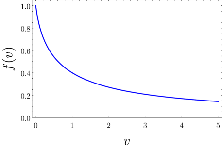
Figure 1: Function $f(v)$ defined in (4.68) that controls the shift to the mass (4.67). Observe that it is smooth everywhere and that it is positive, meaning that the mass is corrected negatively, in agreement with the mild form of the WGC.

4.4.4 Case 2-1: $\beta=-\beta_{0}$ and $q=q_{0}$

It is worth mentioning that, despite the apparent singularity of the previous solution at $q=q_{0}$, the the limit $q\rightarrow q_{0}$ is well-defined, and the solution simplifies greatly in that case:

$$\delta\mathcal{Z}_{0} =-\frac{1}{120q_{0}(r+q_{0})^{3}}\left(12r^{2}+45q_{0}r+65q_{0}^{2}\right)\,,$$ (4.72a)

$$\delta\mathcal{Z}_{0h} =0\,,$$ (4.72b)

$$\delta\mathcal{H} =\delta\mathcal{Z}_{0}\,,$$ (4.72c)

$$\delta\mathcal{Z}_{+} =\frac{q_{+}}{q_{-}}\delta\mathcal{Z}_{-}+(\beta_{+}\beta_{-}+1)\frac{q_{+}\left[(r+q_{-})(2r+q_{0})+q_{0}^{2}\right)}{4q_{0}^{2}(r+q_{-})(r+q_{0})^{2}}\,,$$ (4.72d)

$$\delta\mathcal{Z}_{-} =\frac{q_{-}}{120q_{0}^{2}(r+q_{0})^{3}}\left(8r^{2}+9q_{0}r+3q_{0}^{2}\right)\,,$$ (4.72e)

$$C_{\phi} =e^{2\hat{\phi}_{\infty}}\left(1-\frac{\alpha^{\prime}}{40q_{0}^{2}}\right)\,.$$ (4.72f)

The mass and the area of the horizon are given by

$$M =\frac{1}{4G_{N}^{(4)}}\left\{\hat{q}_{+}+\hat{q}_{-}+2q_{0}-\frac{\alpha^{\prime}}{5q_{0}}\right\}\,,$$ (4.73a)

$$A =4\pi\sqrt{\hat{q}_{+}\hat{q}_{-}q_{0}q}\left\{1-\frac{\alpha^{\prime}}{40q_{0}^{2}}\right\}\,.$$ (4.73b)

4.5 $\alpha^{\prime}$-corrected entropy

The computation of the black hole entropy parallels that of section 3.5. From the equation (3.36), one can see that the Wald entropy can be expressed as

$$S=\frac{A}{4G_{N}^{(4)}}+\Delta S\,.$$ (4.74)

The area term $A/(4G_{N}^{(4)})$ has been computed in Eqs. (4.50b) and (4.70) for the $\beta=\beta_{0}$ and $\beta=-\beta_{0}$ cases, respectively. In terms of the original charge parameters, it is given by

$$A=\frac{4\pi e^{2{\hat{\phi}}_{\infty}}}{C_{\phi}}\sqrt{q_{+}q_{-}q_{0}q}\,,$$ (4.75)

where the constant $C_{\phi}$ is given by (4.36d) and (4.52f) in each case.

On the other hand, $\Delta S$, the correction to the Bekenstein-Hawking entropy, is given by

$$\Delta S=-\frac{\alpha^{\prime}}{16G_{N}^{(10)}}\int_{\Sigma}e^{-2(\hat{\phi}-{\hat{\phi}}_{\infty})}\hat{\star}{\hat{H}}^{(0)}\wedge{\hat{\Omega}}^{(0)}_{(-)}{}^{ab}{\hat{n}}_{ab}\,,$$ (4.76)

where the integral is taken at $r=0$ and where, in the Zehnbein basis in Eqs. (4.4), the only non-vanishing component of the binormal is ${\hat{n}}^{01}=-{\hat{n}}_{01}=+1$. It is important to note that, in the limit $r\rightarrow 0$, we have

$$\lim_{r\rightarrow 0}{\hat{\Omega}}^{(0)}_{(-)}{}^{01} =\frac{1}{\sqrt{q_{0}q}}{\hat{e}}^{t}-\frac{\left(\beta_{+}+\beta_{-}\right)}{\sqrt{q_{0}q}}{\hat{e}}^{z}\,,$$ (4.77)

$$\lim_{r\rightarrow 0}e^{-2(\hat{\phi}-{\hat{\phi}}_{\infty})} =\frac{q_{-}}{q_{0}}e^{2\hat{\phi}_{\infty}}C_{\phi}^{-1}\,.$$ (4.78)

Integrating over the angular and compact variables we obtain that, for both cases $\beta_{0}\beta=\pm 1$, $\Delta S$ is given by

$$\Delta S=\frac{\alpha^{\prime}\pi e^{2{\hat{\phi}}_{\infty}}}{4C_{\phi}G_{N}^{(4)}}\sqrt{\frac{q_{+}q_{-}}{q_{0}q}}(\beta_{+}\beta_{-}+1)\,.$$ (4.79)

Putting together both contributions, we find that the entropy reads

$$S=\frac{\pi e^{2\hat{\phi}_{\infty}}}{C_{\phi}G_{N}^{(4)}}\sqrt{q_{+}q_{-}q_{0}q}\left(1+\frac{\alpha^{\prime}(\beta_{+}\beta_{-}+1)}{4q_{0}q}\right)\,,$$ (4.80)

and we need to express it in terms of the charges $\hat{\mathcal{Q}}_{i}$, which are defined by Eq. (4.49). The relations between the charges and the $q_{i}$ parameters can be written jointly for the $\beta_{0}\beta=+1$ and $\beta_{0}\beta=-1$ cases as

$$\hat{\mathcal{Q}}_{+} =\beta_{+}\frac{2\ell_{\infty}k_{\infty}^{2}}{\ell_{s}C_{\phi}}q_{+}\left[1+\frac{\alpha^{\prime}(\beta_{+}\beta_{-}+1)}{4q_{0}q}\right]\,,$$ (4.81)

$$\hat{\mathcal{Q}}_{-} =\beta_{-}\frac{2\ell_{\infty}}{\ell_{s}C_{\phi}}q_{-}\,,$$

$$\hat{\mathcal{Q}}_{0} =\beta_{0}\frac{2\ell_{\infty}}{\ell_{s}}q_{0}\left[1-\frac{\alpha^{\prime}(\beta_{0}\beta+1)}{4q_{0}q}\right]\,,$$

$$\hat{\mathcal{Q}} =\beta\frac{2}{\ell_{\infty}\ell_{s}}q\,,$$

Inserting these relations in Eq. (4.80), we find the following expression for the entropy,

$$S=2\pi\sqrt{|\hat{\mathcal{Q}}_{+}\hat{\mathcal{Q}}_{-}|(|\hat{\mathcal{Q}}_{0}\hat{\mathcal{Q}}|+2+\beta_{+}\beta_{-}+\beta_{0}\beta)}\,.$$ (4.82)

Let us comment on this result. First, observe that the entropy is trivially invariant under the T duality transformations $\hat{\mathcal{Q}}_{+}\leftrightharpoons\hat{\mathcal{Q}}_{-}$ or $\hat{\mathcal{Q}}_{0}\leftrightharpoons\hat{\mathcal{Q}}$. Second, note that in the supersymmetric case $\beta_{+}\beta_{-}=\beta_{0}\beta=1$, our result matches exactly the microscopic value of the entropy that can be obtained from [62], which is supposed to be $\alpha^{\prime}$-exact. In fact, we reproduce the famous $+4$ term of [62] inside the square root. This result also matches those of Refs. [17, 2, 18, 41, 55] obtained from the application of the entropy function method and the one in [40] from the application of the Lorentz-invariant Wald formula (3.36). The supersymmetry-breaking case $\beta_{+}\beta_{-}=-1$, $\beta_{0}\beta=1$ has also been studied in the literature by means of the entropy function method, and our result matches the $+2$ factor of Ref. [2] (see also [17, 18]). Finally the cases with $\beta_{0}\beta=-1$ do not seem to have been studied in the literature, but we see that when $\beta_{+}\beta_{-}=1$ we get again the $+2$ factor, while if we break supersymmetry twice, $\beta_{+}\beta_{-}=-1$ , then there is no correction to the zeroth-order entropy. Thus, the more ways we break supersymmetry, the smaller the entropy. For a fixed value of the absolute values of the charges, the supersymmetric solution is the most entropic one.

5 $\alpha^{\prime}$-corrected T duality

During the last three decades, the invariance of the zeroth-order in $\alpha^{\prime}$ string effective action under Buscher’s T duality transformations [63, 64] and its type II generalizations [65] has been profusely used as a solution-generating technique. In contrast, the generalization of the rules to first order in $\alpha^{\prime}$ in the context of the heterotic superstring effective action [56] (see also [39]) has not, essentially because almost no solutions to the first-order equations had been found until the $\alpha^{\prime}$ corrections to the Strominger-Vafa black hole were computed in Ref. [10]. The first-order in $\alpha^{\prime}$ T duality rules of Ref. [56] were tested in this solution as well as in the 4-dimensional 4-charge solution of Ref. [12]. Since these solutions, as a family, are expected to be invariant under T duality (only the charges and moduli are transformed, while the functional form of the solution remains invariant) T duality provided a test of the transformations and of the corrections.

The solutions considered in this paper are various non-supersymmetric generalizations of the solutions considered in Refs. [10, 12]. They are expected to be invariant under T duality and this condition can, again, be used to test the corrections found. We have, indeed, checked that the solutions can be written in manifestly T duality-invariant forms in a highly non-trivial way.

Inspired by our results, in this section we are going to show that T duality can be used to constrain the form of the first-order in $\alpha^{\prime}$ corrections when we do not know them. In some cases, these constraints essentially determine the corrections. This fact can be used to simplify the problem of finding the corrections. The key to this result is the fact that the definitions of some of the lower-dimensional fields that transform nicely under T duality (actually, all those descending from the 10-dimensional Kalb-Ramond 2-form) contain $\alpha^{\prime}$ corrections while the rest, do not. This means that the corrections to the latter in the solutions must be related to the corrections to the definitions of the former. This mechanism will become clearer when we study the particular cases.

Let us consider the 5-dimensional case first.

5.1 T duality of the 5-dimensional solutions

We are going to start by assuming that there is a choice of charge parameters whose T duality transformations do not involve $\alpha^{\prime}$ corrections. In the case at hands, these are the hatted charge parameters $\hat{q}_{\pm,0}$ and they are such that the $\mathcal{Z}_{\pm,0}$ functions can be written in the form

$$\mathcal{Z}_{\pm,0}=1+\frac{\hat{q}_{\pm,0}}{\rho^{2}}+\alpha^{\prime}\delta\mathcal{Z}_{\pm,0}\equiv\mathcal{Z}_{\pm,0}^{(0)}+\alpha^{\prime}\delta\mathcal{Z}_{\pm,0}\,.$$ (5.1)

Substituting this expression into the 5-dimensional form of the ansatz Eqs. (3.15) and in Eqs. (3.18) and using the modified-Einstein-frame metric (3.19), we find

$$ds_{E}^{2} =f^{(0)\,2}\left[1-\frac{2\alpha^{\prime}}{3}\left(\frac{\delta\mathcal{Z}_{+}}{\mathcal{Z}^{(0)}_{+}}+\frac{\delta\mathcal{Z}_{-}}{\mathcal{Z}^{(0)}_{-}}+\frac{\delta\mathcal{Z}_{0}}{\mathcal{Z}^{(0)}_{0}}\right)\right]dt^{2}$$

$$\hskip 14.22636pt-f^{(0)\,-1}\left[1+\frac{\alpha^{\prime}}{3}\left(\frac{\delta\mathcal{Z}_{+}}{\mathcal{Z}^{(0)}_{+}}+\frac{\delta\mathcal{Z}_{-}}{\mathcal{Z}^{(0)}_{-}}+\frac{\delta\mathcal{Z}_{0}}{\mathcal{Z}^{(0)}_{0}}\right)\right]\left(d\rho^{2}+\rho^{2}d\Omega_{(3)}^{2}\right)\,,$$ (5.2a)

$$H^{(1)} =-\beta_{0}\left(\hat{q}_{0}-\alpha^{\prime}\rho^{3}\delta\mathcal{Z}_{0}^{\prime}\right)\omega_{(3)}\,,$$ (5.2b)

$$A =\beta_{+}k_{\infty}^{-1}\left[-1+\frac{1}{\mathcal{Z}^{(0)}_{+}}\left(1-\alpha^{\prime}\frac{\delta\mathcal{Z}_{+}}{\mathcal{Z}^{(0)}_{+}}\right)\right]dt\,,$$ (5.2c)

$$B^{(1)} =\beta_{-}k_{\infty}\left\{-1+\frac{1}{\mathcal{Z}^{(0)}_{-}}\left[1+\alpha^{\prime}\left(\Delta^{(0)}-\frac{\delta\mathcal{Z}_{-}}{\mathcal{Z}^{(0)}_{-}}\right)\right]\right\}dt\,,$$ (5.2d)

$$e^{-2\phi} =e^{-2\phi_{\infty}}\frac{\sqrt{\mathcal{Z}^{(0)}_{+}\mathcal{Z}^{(0)}_{-}}}{\mathcal{Z}^{(0)}_{0}}\left\{1+\frac{\alpha^{\prime}}{2}\left(\frac{\delta\mathcal{Z}_{+}}{\mathcal{Z}^{(0)}_{+}}+\frac{\delta\mathcal{Z}_{-}}{\mathcal{Z}^{(0)}_{-}}-2\frac{\delta\mathcal{Z}_{0}}{\mathcal{Z}^{(0)}_{0}}\right)\right\}\,,$$ (5.2e)

$$k =k_{\infty}\sqrt{\frac{\mathcal{Z}^{(0)}_{+}}{\mathcal{Z}^{(0)}_{-}}}\left\{1+\frac{\alpha^{\prime}}{2}\left(\frac{\delta\mathcal{Z}_{+}}{\mathcal{Z}^{(0)}_{+}}-\frac{\delta\mathcal{Z}_{-}}{\mathcal{Z}^{(0)}_{-}}\right)\right\}\,,$$ (5.2f)

$$k^{(1)} =k_{\infty}\sqrt{\frac{\mathcal{Z}^{(0)}_{+}}{\mathcal{Z}^{(0)}_{-}}}\left\{1+\frac{\alpha^{\prime}}{2}\left(\frac{\delta\mathcal{Z}_{+}}{\mathcal{Z}^{(0)}_{+}}-\frac{\delta\mathcal{Z}_{-}}{\mathcal{Z}^{(0)}_{-}}+2\Delta^{(0)}\right)\right\}\,.$$ (5.2g)

where

$$f^{(0)\,-1} =\left(\mathcal{Z}^{(0)}_{+}\mathcal{Z}^{(0)}_{-}\mathcal{Z}^{(0)}_{0}\right)^{1/3}=\frac{1}{\rho^{2}}\left[(\rho^{2}+\hat{q}_{+})(\rho^{2}+\hat{q}_{-})(\rho^{2}+\hat{q}_{0})\right]^{1/3}\,,$$ (5.3a)

$$\Delta^{(0)} =\tfrac{1}{4}(1+\beta_{+}\beta_{-})\frac{\mathcal{Z}^{(0)\,\prime}_{+}\mathcal{Z}^{(0)\,\prime}_{-}}{\mathcal{Z}^{(0)}_{0}\mathcal{Z}^{(0)}_{+}\mathcal{Z}^{(0)}_{-}}=\frac{(1+\beta_{+}\beta_{-})\hat{q}_{+}\hat{q}_{-}}{(\rho^{2}+\hat{q}_{+})(\rho^{2}+\hat{q}_{-})(\rho^{2}+\hat{q}_{0})}\,.$$ (5.3b)

T duality along the internal $z$ direction interchanges the 5-dimensional KK and winding vectors $A$ and $B^{(1)}$ and transforms $k$ into $k^{(1)\,-1}$, leaving the rest of the fields invariant [39]. The invariance of the ansatz under these transformations implies that they are equivalent to the transformations of the parameters in Eq. (3.33). The functions $f^{(0)}$ and $\Delta^{(0)}$ are invariant under these transformations. As for the corrections $\delta\mathcal{Z}_{\pm,0}$, they must transform according to

$$\delta\mathcal{Z}_{\pm}^{\prime}=\delta\mathcal{Z}_{\mp}\mp\Delta^{(0)}\mathcal{Z}^{(0)}_{\mp}\,,$$ (5.4)

while $\delta\mathcal{Z}_{0}$ remains invariant, in agreement with Eq. (3.27a). An equivalent expression of the same result is that the combination

$$\frac{\delta\mathcal{Z}_{+}}{\mathcal{Z}_{+}^{(0)}}-\frac{\delta\mathcal{Z}_{-}}{\mathcal{Z}_{-}^{(0)}}+\Delta^{(0)}\,,$$ (5.5)

must be odd under T duality.

Then, if we find that $\delta\mathcal{Z}_{-}=0$, we automatically know $\delta\mathcal{Z}_{+}$, which is given by

$$\delta\mathcal{Z}_{+}=\Delta^{(0)}\mathcal{Z}^{(0)}_{-}\,,$$ (5.6)

in agreement with Eq. (3.27b).

5.2 T duality of the 4-dimensional solutions

Under the same assumptions made in the 5-dimensional case for the functions $\mathcal{Z}_{\pm,0},\mathcal{H}$, and expanding the constant $C_{\phi}$ as

$$C_{\phi}=e^{2\phi_{\infty}}\left(1+\alpha^{\prime}\delta C\right)\,,$$ (5.7)

we can rewrite the non-vanishing fields of the ansatz for the 4-dimensional solutions in Eqs. (4.27) as

$$ds_{E}^{2} =e^{2U^{(0)}}\left[1-\frac{\alpha^{\prime}}{2}\left(-2\delta C-2\frac{\delta q_{-}}{q_{-}}+2\frac{r^{2}\delta\mathcal{Z}_{-}^{\prime}}{\hat{q}_{-}}+\frac{\delta\mathcal{Z}_{+}}{\mathcal{Z}^{(0)}_{+}}+\frac{\delta\mathcal{Z}_{-}}{\mathcal{Z}^{(0)}_{-}}+\frac{\delta\mathcal{Z}_{0}}{\mathcal{Z}^{(0)}_{0}}+\frac{\delta\mathcal{H}}{\mathcal{H}^{(0)}}\right)\right]dt^{2}$$

$$\hskip 14.22636pt-e^{2U^{(0)}}\left[1+\frac{\alpha^{\prime}}{2}\left(2\delta C+2\frac{\delta q_{-}}{q_{-}}-2\frac{r^{2}\delta\mathcal{Z}_{-}^{\prime}}{\hat{q}_{-}}+\frac{\delta\mathcal{Z}_{+}}{\mathcal{Z}^{(0)}_{+}}+\frac{\delta\mathcal{Z}_{-}}{\mathcal{Z}^{(0)}_{-}}+\frac{\delta\mathcal{Z}_{0}}{\mathcal{Z}^{(0)}_{0}}+\frac{\delta\mathcal{H}}{\mathcal{H}^{(0)}}\right)\right]\times$$

$$\hskip 14.22636pt\times\left(dr^{2}+r^{2}d\Omega^{2}_{(2)}\right)\,,$$ (5.8a)

$$A^{w} =\beta q\ell^{-1}_{\infty}\cos{\theta}d\varphi\,,$$ (5.8b)

$$A^{z} =\beta_{+}k^{-1}_{\infty}\left[-1+\frac{1}{\mathcal{Z}^{(0)}_{+}}\left(1-\alpha^{\prime}\frac{\delta\mathcal{Z}_{+}}{\mathcal{Z}^{(0)}_{+}}\right)\right]dt\,,$$ (5.8c)

$$B^{(1)}{}_{w} =\beta_{0}\ell_{\infty}\hat{q}_{0h}\cos{\theta}d\varphi\,,$$ (5.8d)

$$B^{(1)}{}_{z} =\beta_{-}k_{\infty}\left\{-1+\frac{1}{\mathcal{Z}^{(0)}_{-}}\left[1+\alpha^{\prime}\left(\Delta^{(0)}-\frac{\delta\mathcal{Z}_{-}}{\mathcal{Z}^{(0)}_{-}}\right)\right]\right\}dt\,,$$ (5.8e)

$$\ell =\ell_{\infty}\sqrt{\frac{\mathcal{Z}^{(0)}_{0}}{\mathcal{H}^{(0)}}}\ \left[1+\frac{\alpha^{\prime}}{2}\left(\frac{\delta\mathcal{Z}_{0}}{\mathcal{Z}^{(0)}_{0}}-\frac{\delta\mathcal{H}}{\mathcal{H}^{(0)}}\right)\right]\,,$$ (5.8f)

$$\ell^{(1)} =\ell_{\infty}\sqrt{\frac{\mathcal{Z}^{(0)}_{0}}{\mathcal{H}^{(0)}}}\ \left[1+\frac{\alpha^{\prime}}{2}\left(\frac{\delta\mathcal{Z}_{0}}{\mathcal{Z}^{(0)}_{0}}-\frac{\delta\mathcal{H}}{\mathcal{H}^{(0)}}+2\Sigma^{(0)}\right)\right]\,,$$ (5.8g)

$$k =k_{\infty}\sqrt{\frac{\mathcal{Z}^{(0)}_{+}}{\mathcal{Z}^{(0)}_{-}}}\left\{1+\frac{\alpha^{\prime}}{2}\left(\frac{\delta\mathcal{Z}_{+}}{\mathcal{Z}^{(0)}_{+}}-\frac{\delta\mathcal{Z}_{-}}{\mathcal{Z}^{(0)}_{-}}\right)\right\}\,,$$ (5.8h)

$$k^{(1)} =k_{\infty}\sqrt{\frac{\mathcal{Z}^{(0)}_{+}}{\mathcal{Z}^{(0)}_{-}}}\left[1+\frac{\alpha^{\prime}}{2}\left(\frac{\delta\mathcal{Z}_{+}}{\mathcal{Z}^{(0)}_{+}}-\frac{\delta\mathcal{Z}_{-}}{\mathcal{Z}^{(0)}_{-}}+2\Delta^{(0)}\right)\right]\,,$$ (5.8i)

$$e^{2\phi} =e^{2\phi^{(0)}}\left[1+\frac{\alpha^{\prime}}{2}\left(2\delta C+2\frac{\delta q_{-}}{q_{-}}-2\frac{r^{2}\delta\mathcal{Z}_{-}^{\prime}}{\hat{q}_{-}}+\frac{\delta\mathcal{Z}_{0}}{\mathcal{Z}^{(0)}_{0}}+\frac{\delta\mathcal{H}}{\mathcal{H}^{(0)}}-\frac{\delta\mathcal{Z}_{+}}{\mathcal{Z}^{(0)}_{+}}-\frac{\delta\mathcal{Z}_{-}}{\mathcal{Z}^{(0)}_{-}}\right)\right]\,,$$ (5.8j)

where we have defined

$$e^{2U^{(0)}} =\left(\mathcal{Z}^{(0)}_{+}\mathcal{Z}^{(0)}_{-}\mathcal{Z}^{(0)}_{0}\mathcal{H}^{(0)}\right)^{1/2}=\frac{1}{r^{2}}\left[(r+\hat{q}_{+})(r+\hat{q}_{-})(r+\hat{q}_{0})(r+\hat{q})\right]\,,$$ (5.9a)

$$\Delta^{(0)} =\tfrac{1}{4}(1+\beta_{+}\beta_{-})\frac{\hat{q}_{+}\hat{q}_{-}}{(r+\hat{q}_{+})(r+\hat{q}_{-})(r+\hat{q}_{0})(r+\hat{q})}\,,$$ (5.9b)

$$\Sigma^{(0)} =-\frac{1}{4(\mathcal{Z}^{(0)}_{0}\mathcal{H}^{(0)})^{3}}\left[(\mathcal{Z}^{(0)\,\prime}_{0}\mathcal{H}^{(0)})^{2}+(\mathcal{Z}^{(0)}_{0}\mathcal{H}^{(0)\,\prime})^{2}+(\beta\beta_{0}-1)\mathcal{Z}^{(0)\,\prime}_{0}\mathcal{H}^{(0)\,\prime}\mathcal{Z}^{(0)}_{0}\mathcal{H}^{(0)}\right]$$

$$=-\frac{1}{4(r+\hat{q}_{0})^{3}(r+\hat{q})^{3}}\left[\hat{q}_{0}^{2}(r+\hat{q})^{2}+\hat{q}^{2}(r+\hat{q}_{0})^{2}+(\beta\beta_{0}-1)\hat{q}_{0}\hat{q}(r+\hat{q}_{0})(r+\hat{q})\right]\,,$$ (5.9c)

$$e^{2\phi^{(0)}} =e^{2\phi_{\infty}}\sqrt{\frac{\mathcal{Z}^{(0)}_{0}\mathcal{H}^{(0)}}{\mathcal{Z}^{(0)}_{+}\mathcal{Z}^{(0)}_{-}}}=e^{2\phi_{\infty}}\sqrt{\frac{(r+\hat{q}_{0})(r+\hat{q})}{(r+\hat{q}_{+})(r+\hat{q}_{-})}}\,.$$ (5.9d)

Observe that, since, in general, $\mathcal{Z}_{0}\neq\mathcal{Z}_{0h}$, we have to distinguish between $\hat{q}_{0}$ and $\hat{q}_{0h}$. The latter only occurs in $B^{(1)}{}_{w}$.

Furthermore, observe that the asymptotic behaviour of the metric and dilaton field are correct only if

$$\delta C+\frac{\delta q_{-}}{q_{-}}=0\,.$$ (5.10)

The solutions described by this ansatz are expected to be invariant under T duality transformations in the internal circles parametrized by the coordinates $w$ and $z$ ( $T_{w}$ and $T_{z}$). Let us start with $T_{w}$.

Invariance under $T_{w}$ interchanges $A^{w}$ and $B^{(1)}{}_{w}$ and $\ell$ and $\ell^{(1)\,-1}$, leaving the rest of the fields invariant. The interchange between $A^{w}$ and $B^{(1)}{}_{w}$ implies that $\hat{q}=q$ and the following transformation

$$\beta\rightleftharpoons\beta_{0}\,\hskip 14.22636pt\hat{q}\rightleftharpoons\hat{q}_{0h}\,,\hskip 14.22636pt\ell_{\infty}\rightleftharpoons\ell_{\infty}^{(1)\,-1}\,.$$ (5.11)

The interchange of $\ell$ and $\ell^{(1)\,-1}$ demands, at the level of charge parameters, the interchange between $\hat{q}$ and $\hat{q}_{0}$ which, in its turn, implies $\hat{q}_{0h}=\hat{q}_{0}$. Furthermore, the transformations of the corrections $\delta\mathcal{Z}_{0}$ and $\delta\mathcal{H}$ must be such that the combination

$$\frac{\delta\mathcal{Z}_{0}}{\mathcal{Z}^{(0)}_{0}}-\frac{\delta\mathcal{H}}{\mathcal{H}^{(0)}}+\Sigma^{(0)}\,,$$ (5.12)

is odd under $T_{w}$.

The invariance of $A^{z}$ and $B_{z}$ leads to the invariance of the corrections $\delta\mathcal{Z}_{\pm}$ under $T_{w}$:

$$\delta\mathcal{Z}_{\pm}^{\prime}=\delta\mathcal{Z}_{\pm}\,.$$ (5.13)

This relation makes $k$ automatically invariant under $T_{w}$ as well.

Finally, taking into account the previous results, the invariance of the dilaton and of the metric function lead to the invariance of the combination

$$\frac{\delta\mathcal{Z}_{0}}{\mathcal{Z}^{(0)}_{0}}+\frac{\delta\mathcal{H}}{\mathcal{H}^{(0)}}\,.$$ (5.14)

Combining this condition with Eq. (5.12) we find

$$\delta\mathcal{Z}_{0}^{\prime} =\delta\mathcal{H}-2\Sigma^{(0)}\mathcal{H}\,,$$ (5.15a)

$$\delta\mathcal{H}^{\prime} =\delta\mathcal{Z}_{0}+2\Sigma^{(0)}\mathcal{Z}_{0}\,.$$ (5.15b)

It can be checked that these relations are satisfied by the corrections we have found. If we use in them additional information such as the vanishing of $\delta\mathcal{H}$, these relations can be used to determine some of the corrections in terms of $\Sigma^{(0)}$.

Let us now consider the effect of $T_{z}$. This transformation interchanges $A^{z}$ and $B^{(1)}{}_{z}$, which implies the following transformation on the parameters of the solution:

$$\hat{q}_{\pm}\rightleftharpoons\hat{q}_{\mp}\,,\hskip 28.45274pt\beta_{\pm}\rightleftharpoons\beta_{\mp}\,,\hskip 28.45274ptk_{\infty}\rightleftharpoons k_{\infty}^{-1}\,,$$ (5.16)

and the same relations between the corrections $\delta\mathcal{Z}_{\pm}$ that we obtained in the 5-dimensional case

$$\delta\mathcal{Z}_{\pm}^{\prime}=\delta\mathcal{Z}_{\mp}\mp\Delta^{(0)}\mathcal{Z}^{(0)}_{\mp}\,,$$ (5.17)

These relations imply the relation we would obtain from the transformation of the KK scalar $k$ and allows the determination of $\delta\mathcal{Z}_{+}$ if we know that $\delta\mathcal{Z}_{-}=0$, for instance. Furthermore, it implies the invariance of the combination

$$\frac{\delta\mathcal{Z}_{+}}{\mathcal{Z}_{+}^{(0)}}+\frac{\delta\mathcal{Z}_{-}}{\mathcal{Z}_{-}^{(0)}}\,,$$ (5.18)

which occurs in the dilaton and metric function. The invariance of these two fields requires

$$\frac{\delta\mathcal{Z}_{0}^{\prime}}{\mathcal{Z}_{0}^{(0)}}+\frac{\delta\mathcal{H}^{\prime}}{\mathcal{H}^{(0)}}=\frac{\delta\mathcal{Z}_{0}}{\mathcal{Z}^{(0)}}+\frac{\delta\mathcal{H}}{\mathcal{H}^{(0)}}-2r^{2}\frac{d~{}}{dr}\left[\frac{\delta\mathcal{Z}_{-}}{q_{-}}-\frac{\delta\mathcal{Z}_{+}}{q_{+}}-\Delta^{(0)}\frac{\mathcal{Z}_{+}}{q_{+}}\right]\,,$$ (5.19)

while the invariance of the KK scalar $\ell$ requires that of

$$\frac{\delta\mathcal{Z}_{0}}{\mathcal{Z}_{0}^{(0)}}-\frac{\delta\mathcal{H}}{\mathcal{H}^{(0)}}\,.$$ (5.20)

Combining these two conditions, we get conditions for $\delta\mathcal{Z}_{0}$ and $\delta\mathcal{H}$ separately

$$\delta\mathcal{Z}_{0}^{\prime}=\delta\mathcal{Z}_{0}-r^{2}\frac{d~{}}{dr}\left[\frac{\delta\mathcal{Z}_{-}}{q_{-}}-\frac{\delta\mathcal{Z}_{+}}{q_{+}}-\Delta^{(0)}\frac{\mathcal{Z}_{+}}{q_{+}}\right]\mathcal{Z}_{0}^{(0)}\,,$$ (5.21a)

$$\delta\mathcal{H}^{\prime}=\delta\mathcal{H}-r^{2}\frac{d~{}}{dr}\left[\frac{\delta\mathcal{Z}_{-}}{q_{-}}-\frac{\delta\mathcal{Z}_{+}}{q_{+}}-\Delta^{(0)}\frac{\mathcal{Z}_{+}}{q_{+}}\right]\mathcal{H}^{(0)}\,.$$ (5.21b)

In the solutions we have found, these conditions are satisfied in an almost trivial fashion, since the term in the derivative vanishes identically and $\delta\mathcal{Z}_{0}$ and $\delta\mathcal{H}$ are invariant under $T_{z}$.

6 Discussion

We have computed the $\alpha^{\prime}$ corrections to a general family of 3- and 4- charge black hole solutions of the heterotic superstring effective action. These corrections are more easily obtained in ten dimensions, where the solutions can be interpreted as a superposition of fundamental strings, momentum waves, solitonic 5-branes, and (in the 4-charge case) Kaluza-Klein monopoles. We have then derived the form of the 4- and 5-dimensional fields by using the results of Ref. [40]. As we have shown, a particular choice of the signs of the charges corresponds to supersymmetric solutions, in which case we recover the results of Refs. [10, 12]. However, any other choice does not preserve any supersymmetry. Interestingly, while at zeroth order in $\alpha^{\prime}$ all these solutions have the same form, the first-order corrections are drastically different depending on the way we break supersymmetry. These differences not only affect the profile of the fields, but also the values of the mass, area, entropy and charges of these extremal black holes. In fact, as we have argued in the text, the identification of the physically relevant charges becomes a non-trivial problem in the presence of $\alpha^{\prime}$ terms. As a practical solution, we have introduced the charge parameters $\hat{\mathcal{Q}}_{i}$ as one would define them in the zeroth-order theory (see Eqs. (3.22) and (4.49)). These charges correspond to the leading coefficients in the asymptotic expansion of the gauge fields in four or five dimensions and they would in principle correspond to Maxwell charges as introduced in [60]. Moreover, it has been checked [41, 55] that these charges match those used in the computation of near-horizon geometries [17, 2, 18], at least in the supersymmetric cases. Thus, they serve us to make contact with previous results. There are, nevertheless, other possible definitions of charges due to the presence of Chen-Simons terms, and it is not clear which ones should be quantized. All these issues clearly deserve further attention.

One of the most important results of this paper is the computation of the black hole entropy in terms of these asymptotic charges. As explained in the introduction, obtaining the $\alpha^{\prime}$-corrected entropy in heterotic string theory has been traditionally problematic due to the Lorentz-Chern-Simons terms in the definition of 3-form field-strength $H$. Here we have performed a rigorous computation of the entropy by using the gauge-invariant generalization of Wald’s formula provided in Ref. [38]. The result, that we repeat here for convenience, reads

$$S=2\pi\sqrt{|\hat{\mathcal{Q}}_{+}\hat{\mathcal{Q}}_{-}|\left(k+2+\beta_{+}\beta_{-}\right)}\,,$$ (6.1)

where

$$k=\begin{cases}|\hat{\mathcal{Q}}_{0}|&\text{if}\,\,D=5\\ |\hat{\mathcal{Q}}_{0}\hat{\mathcal{Q}}|+\beta_{0}\beta&\text{if}\,\,D=4\,,\end{cases}$$ (6.2)

and where $\beta_{i}=\operatorname{sign}{(\hat{\mathcal{Q}}_{i})}$ is the sign of the corresponding charge. The $D=5$ result matches the one in Ref. [18] using the entropy function method, provided one relates $|\hat{\mathcal{Q}}_{0}|$ with the number of S5-branes correctly. The supersymmetric case also matches the corrections to the statistical entropy obtained in Ref. [3]. The $D=4$ result in the supersymmetric case $\beta_{0}\beta=\beta_{+}\beta_{-}=1$ matches exactly previous microscopic results [62, 67, 2]. It also matches the results of refs. [17, 2, 18, 41, 55] that applied the entropy function method for the cases $\beta_{0}\beta=1$ and arbitrary $\beta_{+}\beta_{-}$. To the best of our knowledge, the case $\beta_{0}\beta=-1$ is new. Although this entropy has been computed from the first-order in $\alpha^{\prime}$ action, it can be argued that it is exact in the $\alpha^{\prime}$ expansion [67, 68, 2]. As a matter of fact, the value of the entropy can be determined from the near-horizon geometry only, and for all the black holes considered here, this is an AdS${}_{3}\times\mathbb{S}^{3}/\mathbb{Z}_{n}\times\mathrm{T}^{4}$ geometry with the peculiarity that the curvature of the torsionful spin connection vanishes, $R_{(-)}=0$. Hence, any higher-order term in the action that contains more than one factor of $R_{(-)}$ will be irrelevant for the entropy. This is certainly the case for the $\mathcal{O}(\alpha^{\prime 3})$ terms introduced by supersymmetry [7]. It cannot be guaranteed that the effective action does not contain other types of terms, but this argument at least protects the entropy from supersymmetry-related higher-derivative corrections.

It is also interesting to look at the mass of these solutions, which receives $\alpha^{\prime}$ corrections. We can analyze this from the viewpoint of the Weak Gravity Conjecture (WGC), according to which, the corrections to the extremality bound should be such that the decay of an extremal black hole into a set of smaller black holes should be possible in terms of charge and energy conservation [19, 20, 21]. This has mostly been applied to theories with a single $\mathrm{U}(1)$ field [22, 23, 24, 25, 13, 26, 27, 28, 29, 30, 31], in which case this is rephrased as the condition that the charge-to-mass ratio of extremal black holes is corrected positively. For dimensionality reasons, four-derivative corrections always modify the charge-to-mass ratio as $Q/M=1+c/Q^{2}+\ldots$, for a certain constant $c$. However, when there are several charges involved, the corrections to the extremal mass can take a more complicated form. Also, in that case one needs to formulate the WGC appropriately [61]. For our black holes we have found that, in most instances, the mass is not corrected when expressed in terms of the asymptotic charges $\hat{\mathcal{Q}}_{i}$. This is the case in particular for supersymmetric black holes. However, the non-supersymmetric solution with $\beta_{0}\beta=-1$ does contain an interesting correction to the mass, given by Eq. (4.67). This depends non-trivially on the charges $\hat{\mathcal{Q}}_{0}$ and $\hat{\mathcal{Q}}$, and we have checked that it is negative for any of their values. Having a negative shift to the mass seems to be the natural generalization of the WGC for this class of black holes, so this result provides a non-trivial check of the validity of the WGC in string theory.

The zeroth-order solutions we have started from, as families of solutions, are invariant under T duality. We have seen how this property is preserved at first order when the first-order T-duality rules of Ref. [56] are used. As a matter of fact, the lower-dimensional solutions can be written in a manifestly T-duality-invariant form using the relations between the higher- and lower-dimensional fields of Ref. [39]. A fundamental property of those relations is the presence of $\alpha^{\prime}$ corrections in them for all the fields descending from the 10-dimensional Kalb-Ramond 2-form. Since these corrections depend only on the zeroth-order fields (at first order) they, automatically, determine part of the $\alpha^{\prime}$ corrections to the solutions and, as we have discussed in Section 5, this fact and T duality can be used to determine some of the first-order $\alpha^{\prime}$ corrections to all the fields.

Finally, we find it worth remarking that, interestingly, some of the solutions that break supersymmetry are simpler than their supersymmetric counterparts. We are referring to the case $\beta_{+}\beta_{-}=-1$, and $\beta_{0}\beta=1$. For that choice of signs, only the function $\mathcal{Z}_{0}$ receives corrections. In addition, we know that those corrections can be cancelled by turning on the non-Abelian gauge fields and introducing one (in $D=5$) or two (in $D=4$) $\mathrm{SU}(2)$ instantons [10, 11, 12]. In that situation, the zeroth-order solution receives no $\alpha^{\prime}$ corrections whatsoever, (except for the presence of the instantons), and this is because the $T$-tensors defined in Eq. (2.9), and that control the $\alpha^{\prime}$ corrections, are identically vanishing. Interestingly, the next-order corrections appear at $\mathcal{O}(\alpha^{\prime 3})$ and they are again built out of these $T$-tensors [7], so they do not modify these solutions either. One could speculate that the full tower of $\alpha^{\prime}$ terms is built out of these tensors, in which case these black holes would be $\alpha^{\prime}$-exact solutions of the Heterotic Superstring effective action. This may actually be the case for the higher-derivative terms that arise from the supersymmetrization of the Lorentz-Chern-Simons terms, which are the ones computed in [7]. However, the effective action could contain other contributions besides those, which would invalidate the claim on the exactness of these solutions. Unfortunately, our current knowledge on the higher-order $\alpha^{\prime}$ terms is too limited to establish a definitive conclusion.

Appendix A Relation between 10- and 9-dimensional fields at $\mathcal{O}(\alpha^{\prime})$

At first order in $\alpha^{\prime}$, the 10-dimensional fields can be expressed in terms of the 9-dimensional ones as follows:

$$\hat{g}_{\mu\nu} =g_{\mu\nu}-k^{2}A_{\mu}A_{\nu}\,,$$ (A.1)

$$\hat{g}_{\mu\underline{z}} =-k^{2}A_{\mu}\,,$$

$$\hat{g}_{\underline{z}\underline{z}} =-k^{2}\,,$$

$$\hat{B}_{\mu\nu} =B^{(1)}{}_{\mu\nu}-A_{[\mu}\left[B^{(1)}{}_{\nu]}+\frac{\alpha^{\prime}}{2}k\left(\varphi_{A}A^{A}{}_{|\nu]}+\tfrac{1}{2}\Omega^{(0)}_{(-)\,|\nu]}{}^{ab}K^{(+)}{}_{ab}-K^{(-)}{}_{|\nu]}{}^{a}\partial_{a}\log{k}\right)\right]\,,$$

$$\hat{B}_{\mu\underline{z}} =B^{(1)}{}_{\mu}+\frac{\alpha^{\prime}}{4}k\left(\varphi_{A}A^{A}{}_{\mu}+\tfrac{1}{2}\Omega^{(0)}_{(-)\,\mu}{}^{ab}K^{(+)}{}_{ab}-K^{(-)}{}_{\mu}{}^{a}\partial_{a}\log{k}\right)\,,$$

$$\hat{\phi} =\phi+\tfrac{1}{2}\log{k}\,,$$

$$\hat{A}^{A}{}_{\mu} =A^{A}{}_{\mu}+k\varphi^{A}A_{\mu}\,,$$

$$\hat{A}^{A}{}_{\underline{z}} =k\varphi^{A}\,.$$

The inverse relations are

$$g_{\mu\nu} =\hat{g}_{\mu\nu}-\hat{g}_{\underline{z}\mu}\hat{g}_{\underline{z}\nu}/\hat{g}_{\underline{z}\underline{z}}\,,$$ (A.2)

$$A_{\mu} =\hat{g}_{\mu\underline{z}}/\hat{g}_{\underline{z}\underline{z}}\,,$$

$$k =|\hat{g}_{\underline{z}\underline{z}}|^{1/2}\,,$$

$$B^{(1)}{}_{\mu\nu} =\hat{B}_{\mu\nu}+\hat{g}_{\underline{z}[\mu}\left[\hat{B}_{|\nu]\,\underline{z}}+\frac{\alpha^{\prime}}{4}\left(\hat{A}^{A}{}_{|\nu]}\hat{A}_{A\,\underline{z}}+\hat{\Omega}^{(0)}_{(-)\,|\nu]}{}^{\hat{a}}{}_{\hat{b}}\hat{\Omega}^{(0)}_{(-)\,\underline{z}}{}^{\hat{b}}{}_{\hat{a}}\right)\right]/\hat{g}_{\underline{z}\underline{z}}\,,$$

$$B^{(1)}{}_{\mu} =\hat{B}_{\mu\,\underline{z}}-\frac{\alpha^{\prime}}{4}\left[\hat{A}^{A}{}_{\mu}\hat{A}_{A\,\underline{z}}+\hat{\Omega}^{(0)}_{(-)\,\mu}{}^{\hat{a}}{}_{\hat{b}}\hat{\Omega}^{(0)}_{(-)\,\underline{z}}{}^{\hat{b}}{}_{\hat{a}}\right.$$

$$\left.-\hat{g}_{\mu\underline{z}}\left(\hat{A}^{A}{}_{\underline{z}}\hat{A}_{A\,\underline{z}}+\hat{\Omega}^{(0)}_{(-)\,\underline{z}}{}^{\hat{a}}{}_{\hat{b}}\hat{\Omega}^{(0)}_{(-)\,\underline{z}}{}^{\hat{b}}{}_{\hat{a}}\right)/\hat{g}_{\underline{z}\underline{z}}\right]\,,$$

$$\phi =\hat{\phi}-\tfrac{1}{4}\log{(-\hat{g}_{\underline{z}\underline{z}})}\,,$$

$$A^{A}{}_{\mu} =\hat{A}^{A}{}_{\mu}-\hat{A}^{A}{}_{\underline{z}}\hat{g}_{\mu\underline{z}}/\hat{g}_{\underline{z}\underline{z}}\,,$$

$$\varphi^{A} =\hat{A}^{A}{}_{\underline{z}}/(-\hat{g}_{\underline{z}\underline{z}})^{1/2}\,.$$

We also use the scalar combination $k^{(1)}$, which is defined as follows:

$$k^{(1)}\equiv k\left[1+\frac{\alpha^{\prime}}{4}\left(\varphi^{2}-\tfrac{1}{4}K^{(+)\,2}+2(\partial\log{k})^{2}\right)\right]\,.$$ (A.3)

In terms of the 10-dimensional fields

$$k^{(1)}\equiv k\left[1-\frac{\alpha^{\prime}}{4}\left(\hat{A}_{A\,\underline{z}}\hat{A}^{A}{}_{\underline{z}}+\hat{\Omega}^{(0)}_{(-)\,\underline{z}}{}^{\hat{a}}{}_{\hat{b}}\hat{\Omega}^{(0)}_{(-)\,\underline{z}}{}^{\hat{b}}{}_{\hat{a}}\right)/\hat{g}_{\underline{z}\underline{z}}\right]\,.$$ (A.4)

Some of these expressions contain implicit $\mathcal{O}(\alpha^{\prime}{}^{2})$ terms which give them a nicer or simpler form. They should be consistently ignored.

Appendix B The coset space SU$(2)/$U$(1)$

The su$(2)$ algebra

$$[T_{i},T_{j}]=-\epsilon_{ijk}T_{k}\,,\hskip 28.45274pti,j,k=1,2,3\,,$$ (B.1)

can be split into horizontal ($P_{a}$) and vertical ($M$) components with the commutation relations

$$[P_{a},P_{b}]=-\epsilon_{ab}M\,,\hskip 28.45274pt[M,P_{a}]=-\epsilon_{ab}P_{b}\,,\hskip 28.45274pta,b=1,2\,.$$ (B.2)

A SU$(2)/$U$(1)$ corset representative, $u$ can be constructed by exponentiation

$$u=e^{x^{1}P_{1}}e^{x^{2}P_{2}}\,,$$ (B.3)

where $x^{a}$ are two coordinates unrelated to those of the main body of this paper.

The left-invariant Maurer-Cartan 1-form is

$$V =-u^{-1}du$$ (B.4)

$$=(-\cos{x^{2}}dx^{1})P_{1}+(-dx^{2})P_{2}+\sin{x^{2}}dx^{1}M$$

$$\equiv v^{a}P_{a}+\vartheta M\,.$$

The horizontal components $v^{a}$ will be used as Zweibeins while the vertical component $\vartheta$ will play the role of U$(1)$ connection. The Maurer-Cartan equations are

$$dV-V\wedge V=0\,,\,\,\,\,\,\Rightarrow\,\,\,\,\,\left\{\begin{array}[]{rcl}dv^{a}&=&-\epsilon^{ab}v^{b}\wedge\vartheta\,,\\ &&\\ d\vartheta&=&-\tfrac{1}{2}\epsilon_{ab}v^{a}\wedge v^{b}\,.\end{array}\right.$$ (B.5)

The coordinates $x^{a}$ are related to the standard $\theta,\varphi$ by

$$x^{2}=\pi/2-\theta\,,\hskip 28.45274ptx^{1}=-\varphi\,,$$ (B.6)

and, in terms of these coordinates

$$v^{1}=\sin{\theta}d\varphi\,,\hskip 14.22636ptv^{2}=d\theta\,,\hskip 14.22636pt\vartheta=-\cos{\theta}d\varphi\,.$$ (B.7)

Using the invariant metric $\delta_{ab}$, we get

$$ds^{2} =\delta_{ab}v^{a}\otimes v^{b}=d\Omega^{2}{}_{(2)}\,,$$ (B.8a)

$$\omega_{(2)} =-\tfrac{1}{2}\epsilon_{ab}v^{a}\wedge v^{b}=\sin{\theta}d\theta\wedge d\varphi\,,$$ (B.8b)

$$d\vartheta =\omega_{(2)}\,.$$ (B.8c)

References

• [1] A. Strominger and C. Vafa, “Microscopic origin of the Bekenstein-Hawking entropy,” Phys. Lett. B 379 (1996), 99-104 DOI:10.1016/0370-2693(96)00345-0 [hep-th/9601029 [hep-th]].
• [2] A. Sen, “Black Hole Entropy Function, Attractors and Precision Counting of Microstates,” Gen. Rel. Grav. 40 (2008), 2249-2431 DOI:10.1007/s10714-008-0626-4 [arXiv:0708.1270 [hep-th]].
• [3] A. Castro and S. Murthy, “Corrections to the statistical entropy of five dimensional black holes,” JHEP 06 (2009), 024 DOI:10.1088/1126-6708/2009/06/024 [arXiv:0807.0237 [hep-th]].
• [4] D. J. Gross and J. H. Sloan, “The Quartic Effective Action for the Heterotic String,” Nucl. Phys. B 291 (1987), 41-89 DOI:10.1016/0550-3213(87)90465-2
• [5] R. R. Metsaev and A. A. Tseytlin, “Curvature Cubed Terms in String Theory Effective Actions,” Phys. Lett. B 185 (1987), 52-58 DOI:10.1016/0370-2693(87)91527-9
• [6] R. R. Metsaev and A. A. Tseytlin, “Order alpha-prime (Two Loop) Equivalence of the String Equations of Motion and the Sigma Model Weyl Invariance Conditions: Dependence on the Dilaton and the Antisymmetric Tensor,” Nucl. Phys. B 293 (1987), 385-419 DOI:10.1016/0550-3213(87)90077-0
• [7] E. A. Bergshoeff and M. de Roo, “The Quartic Effective Action of the Heterotic String and Supersymmetry,” Nucl. Phys. B 328 (1989) 439. DOI:10.1016/0550-3213(89)90336-2
• [8] B. A. Campbell, N. Kaloper and K. A. Olive, “Classical hair for Kerr-Newman black holes in string gravity,” Phys. Lett. B 285 (1992), 199-205 DOI:10.1016/0370-2693(92)91452-F
• [9] M. Natsuume, “Higher order correction to the GHS string black hole,” Phys. Rev. D 50 (1994), 3949-3953 DOI:10.1103/PhysRevD.50.3949 [hep-th/9406079 [hep-th]].
• [10] P. A. Cano, P. Meessen, T. Ortín and P. F. Ramírez, “$\alpha^{\prime}$-corrected black holes in String Theory,” JHEP 05 (2018), 110 DOI:10.1007/JHEP05(2018)110 [arXiv:1803.01919 [hep-th]].
• [11] S. Chimento, P. Meessen, T. Orín, P. F. Ramírez and A. Ruipérez, “On a family of $\alpha^{\prime}$-corrected solutions of the Heterotic Superstring effective action,” JHEP 07 (2018), 080 DOI:10.1007/JHEP07(2018)080 [arXiv:1803.04463 [hep-th]].
• [12] P. A. Cano, S. Chimento, P. Meessen, T. Ortín, P. F. Ramírez and A. Ruipérez, “Beyond the near-horizon limit: Stringy corrections to Heterotic Black Holes,” JHEP 02 (2019), 192 DOI:10.1007/JHEP02(2019)192 [arXiv:1808.03651 [hep-th]].
• [13] P. A. Cano, S. Chimento, R. Linares, T. Ortín and P. F. Ramírez, “$\alpha^{\prime}$ corrections of Reissner-Nordström black holes,” JHEP 02 (2020), 031 DOI:10.1007/JHEP02(2020)031 [arXiv:1910.14324 [hep-th]].
• [14] P. A. Cano and A. Ruipérez, “String gravity in $D=4$,” [arXiv:2111.04750 [hep-th]].
• [15] A. Sen, “Black hole entropy function and the attractor mechanism in higher derivative gravity,” JHEP 09 (2005), 038 DOI:10.1088/1126-6708/2005/09/038 [hep-th/0506177 [hep-th]].
• [16] T. Ortín, “Extremality versus supersymmetry in stringy black holes,” Phys. Lett. B 422 (1998), 93-100 DOI:10.1016/S0370-2693(98)00040-9 [hep-th/9612142 [hep-th]].
• [17] B. Sahoo and A. Sen, “alpha-prime - corrections to extremal dyonic black holes in heterotic string theory,” JHEP 01 (2007), 010 DOI:10.1088/1126-6708/2007/01/010 [hep-th/0608182 [hep-th]].
• [18] P. Dominis Prester and T. Terzic, “$\alpha^{\prime}$-exact entropies for BPS and non-BPS extremal dyonic black holes in heterotic string theory from ten-dimensional supersymmetry,” JHEP 0812 (2008) 088. DOI:10.1088/1126-6708/2008/12/088 [arXiv:0809.4954 [hep-th]].
• [19] Y. Kats, L. Motl and M. Padi, “Higher-order corrections to mass-charge relation of extremal black holes,” JHEP 12 (2007), 068 DOI:10.1088/1126-6708/2007/12/068 [hep-th/0606100 [hep-th]].
• [20] C. Cheung, J. Liu and G. N. Remmen, “Proof of the Weak Gravity Conjecture from Black Hole Entropy,” JHEP 10 (2018), 004 DOI:10.1007/JHEP10(2018)004 [arXiv:1801.08546 [hep-th]].
• [21] Y. Hamada, T. Noumi and G. Shiu, “Weak Gravity Conjecture from Unitarity and Causality,” Phys. Rev. Lett. 123 (2019) no.5, 051601 DOI:10.1103/PhysRevLett.123.051601 [arXiv:1810.03637 [hep-th]].
• [22] L. Aalsma, A. Cole and G. Shiu, “Weak Gravity Conjecture, Black Hole Entropy, and Modular Invariance,” JHEP 08 (2019), 022 DOI:10.1007/JHEP08(2019)022 [arXiv:1905.06956 [hep-th]].
• [23] B. Bellazzini, M. Lewandowski and J. Serra, “Positivity of Amplitudes, Weak Gravity Conjecture, and Modified Gravity,” Phys. Rev. Lett. 123 (2019) no.25, 251103 doi:10.1103/PhysRevLett.123.251103 [arXiv:1902.03250 [hep-th]].
• [24] S. Cremonini, C. R. T. Jones, J. T. Liu and B. McPeak, “Higher-Derivative Corrections to Entropy and the Weak Gravity Conjecture in Anti-de Sitter Space,” JHEP 09 (2020), 003 DOI:10.1007/JHEP09(2020)003 [arXiv:1912.11161 [hep-th]].
• [25] A. M. Charles, “The Weak Gravity Conjecture, RG Flows, and Supersymmetry,” [arXiv:1906.07734 [hep-th]].
• [26] G. J. Loges, T. Noumi and G. Shiu, “Thermodynamics of 4D Dilatonic Black Holes and the Weak Gravity Conjecture,” Phys. Rev. D 102 (2020) no.4, 046010 DOI:10.1103/PhysRevD.102.046010 [arXiv:1909.01352 [hep-th]].
• [27] S. Andriolo, T. C. Huang, T. Noumi, H. Ooguri and G. Shiu, “Duality and axionic weak gravity,” Phys. Rev. D 102 (2020) no.4, 046008 DOI:10.1103/PhysRevD.102.046008 [arXiv:2004.13721 [hep-th]].
• [28] G. J. Loges, T. Noumi and G. Shiu, “Duality and Supersymmetry Constraints on the Weak Gravity Conjecture,” JHEP 11 (2020), 008 DOI:10.1007/JHEP11(2020)008 [arXiv:2006.06696 [hep-th]].
• [29] P. A. Cano and Á. Murcia, “Electromagnetic Quasitopological Gravities,” JHEP 10 (2020), 125 DOI:10.1007/JHEP10(2020)125 [arXiv:2007.04331 [hep-th]].
• [30] P. A. Cano and Á. Murcia, “Duality-invariant extensions of Einstein-Maxwell theory,” DOI:10.1007/JHEP08(2021)042 [arXiv:2104.07674 [hep-th]].
• [31] N. Arkani-Hamed, Y. t. Huang, J. Y. Liu and G. N. Remmen, “Causality, Unitarity, and the Weak Gravity Conjecture,” [arXiv:2109.13937 [hep-th]].
• [32] P. A. Cano, T. Ortín and P. F. Ramírez, “On the extremality bound of stringy black holes,” JHEP 02 (2020), 175 DOI:10.1007/JHEP02(2020)175 [arXiv:1909.08530 [hep-th]].
• [33] J. Lee and R. M. Wald, “Local symmetries and constraints,” J. Math. Phys. 31 (1990), 725-743 DOI:10.1063/1.528801
• [34] R. M. Wald, “Black hole entropy is the Noether charge,” Phys. Rev. D 48 (1993) no.8, R3427. DOI:10.1103/PhysRevD.48.R3427 [gr-qc/9307038].
• [35] V. Iyer and R. M. Wald, “Some properties of Noether charge and a proposal for dynamical black hole entropy,” Phys. Rev. D 50 (1994) 846. DOI:10.1103/PhysRevD.50.846 [gr-qc/9403028].
• [36] Z. Elgood, P. Meessen and T. Ortín, “The first law of black hole mechanics in the Einstein-Maxwell theory revisited,” JHEP 09 (2020), 026 DOI:10.1007/JHEP09(2020)026 [arXiv:2006.02792 [hep-th]].
• [37] Z. Elgood, D. Mitsios, T. Ortín and D. Pereñíguez, “The first law of heterotic stringy black hole mechanics at zeroth order in $\alpha$’,” JHEP 07 (2021), 007 DOI:10.1007/JHEP07(2021)007 [arXiv:2012.13323 [hep-th]].
• [38] Z. Elgood, T. Ortín and D. Pereñíguez, “The first law and Wald entropy formula of heterotic stringy black holes at first order in $\alpha^{\prime}$,” JHEP 05 (2021), 110 DOI::10.1007/JHEP05(2021)110 [arXiv:2012.14892 [hep-th]].
• [39] Z. Elgood and T. Ortin, “T duality and Wald entropy formula in the Heterotic Superstring effective action at first-order in $\alpha$’,” JHEP 10 (2020), 097 [erratum: JHEP 06 (2021), 105] DOI:10.1007/JHEP10(2020)097 [arXiv:2005.11272 [hep-th]].
• [40] T. Ortín, “O(n,n) invariance and Wald entropy formula in the Heterotic Superstring effective action at first order in $\alpha^{\prime}$,” JHEP 01 (2021), 187 DOI:10.1007/JHEP01(2021)187 [arXiv:2005.14618 [hep-th]].
• [41] F. Faedo and P. F. Ramírez, “Exact charges from heterotic black holes,” JHEP 10 (2019), 033. DOI:10.1007/JHEP10(2019)033 [arXiv:1906.12287 [hep-th]].
• [42] T. Ortín, A. Ruipérez and M. Zatti, work in progress.
• [43] C. G. Callan and J. M. Maldacena, “D-brane approach to black hole quantum mechanics,” Nucl. Phys. B 472 (1996), 591-610 DOI:10.1016/0550-3213(96)00225-8 [hep-th/9602043 [hep-th]].
• [44] A. A. Tseytlin, “Extreme dyonic black holes in string theory,” Mod. Phys. Lett. A 11 (1996), 689-714 DOI:10.1142/S0217732396000709 [hep-th/9601177 [hep-th]].
• [45] M. Cvetic and D. Youm, “General rotating five-dimensional black holes of toroidally compactified heterotic string,” Nucl. Phys. B 476 (1996), 118-132 DOI:10.1016/0550-3213(96)00355-0 [hep-th/9603100 [hep-th]].
• [46] M. Cvetic and D. Youm, “All the static spherically symmetric black holes of heterotic string on a six torus,” Nucl. Phys. B 472, 249-267 (1996) DOI:10.1016/0550-3213(96)00219-2 [hep-th/9512127 [hep-th]].
• [47] J. M. Maldacena and A. Strominger, “Statistical entropy of four-dimensional extremal black holes,” Phys. Rev. Lett. 77 (1996), 428-429 DOI:10.1103/PhysRevLett.77.428 [hep-th/9603060 [hep-th]].
• [48] C. V. Johnson, R. R. Khuri and R. C. Myers, “Entropy of 4-D extremal black holes,” Phys. Lett. B 378 (1996), 78-86 DOI:10.1016/0370-2693(96)00383-8 [hep-th/9603061 [hep-th]].
• [49] T. Ortín, “Gravity and Strings”, 2nd edition, Cambridge University Press, 2015.
• [50] A. Fontanella and T. Ortín, “On the supersymmetric solutions of the Heterotic Superstring effective action,” JHEP 06 (2020), 106 DOI:10.1007/JHEP06(2020)106 [arXiv:1910.08496 [hep-th]].
• [51] N. Alonso-Alberca, E. Lozano-Tellechea and T. Ortín, “Geometric construction of Killing spinors and supersymmetry algebras in homogeneous space-times,” Class. Quant. Grav. 19 (2002), 6009-6024 DOI:10.1088/0264-9381/19/23/309 [hepth0208158 [hep-th]].
• [52] J. M. Maldacena, “Black holes in string theory,” PhD Thesis [hep-th/9607235 [hep-th]].
• [53] G. Papadopoulos, “New half supersymmetric solutions of the heterotic string,” Class. Quant. Grav. 26, 135001 (2009) DOI:10.1088/0264-9381/26/13/135001 [arXiv:0809.1156 [hep-th]].
• [54] A. Ruipérez, “Higher-derivative corrections to small black rings,” Class. Quant. Grav. 38, no.14, 145011 (2021) DOI:10.1088/1361-6382/abff9b [arXiv:2003.02269 [hep-th]].
• [55] P. A. Cano, Á. Murcia, P. F. Ramírez and A. Ruipérez, “On small black holes, KK monopoles and solitonic 5-branes,” JHEP 05 (2021), 272 DOI:10.1007/JHEP05(2021)272 [arXiv:2102.04476 [hep-th]].
• [56] E. Bergshoeff, B. Janssen and T. Ortín, “Solution generating transformations and the string effective action,” Class. Quant. Grav.  13 (1996) 321. DOI:10.1088/0264-9381/13/3/002 [hep-th/9506156].
• [57] T. Jacobson, G. Kang and R. C. Myers, “On black hole entropy,” Phys. Rev. D 49 (1994), 6587-6598 DOI:10.1103/PhysRevD.49.6587 [grqc9312023 [gr-qc]].
• [58] S. Ferrara, G. W. Gibbons and R. Kallosh, “Black holes and critical points in moduli space,” Nucl. Phys. B 500 (1997), 75-93 DOI:10.1016/S0550-3213(97)00324-6 [hep-th/9702103 [hep-th]].
• [59] P. A. Cano, S. Chimento, T. Ortín and A. Ruipérez, “Regular Stringy Black Holes?,” Phys. Rev. D 99 (2019) no.4, 046014 DOI:10.1103/PhysRevD.99.046014 [arXiv:1806.08377 [hep-th]].
• [60] D. Marolf, “Chern-Simons terms and the three notions of charge,” [hep-th/0006117 [hep-th]].
• [61] C. R. T. Jones and B. McPeak, “The Black Hole Weak Gravity Conjecture with Multiple Charges,” JHEP 06 (2020), 140 DOI:10.1007/JHEP06(2020)140 [arXiv:1908.10452 [hep-th]].
• [62] D. Kutasov, F. Larsen and R. G. Leigh, “String theory in magnetic monopole backgrounds,” Nucl. Phys. B 550 (1999), 183-213 DOI:10.1016/S0550-3213(99)00144-3 [hep-th/9812027 [hep-th]].
• [63] T. H. Buscher, “A Symmetry of the String Background Field Equations,” Phys. Lett. B 194 (1987) 59. DOI:10.1016/0370-2693(87)90769-6
• [64] T. H. Buscher, “Path Integral Derivation of Quantum Duality in Nonlinear Sigma Models,” Phys. Lett. B 201 (1988) 466. DOI:10.1016/0370-2693(88)90602-8
• [65] E. Bergshoeff, C. M. Hull and T. Ortín, “Duality in the type II superstring effective action,” Nucl. Phys. B 451 (1995), 547-578 DOI:10.1016/0550-3213(95)00367-2 [hepth9504081 [hep-th]].
• [66] P. A. Cano, P. F. Ramírez and A. Ruipérez, “The small black hole illusion,” JHEP 03 (2020), 115 DOI:10.1007/JHEP03(2020)115 [arXiv:1808.10449 [hep-th]].
• [67] P. Kraus and F. Larsen, “Microscopic black hole entropy in theories with higher derivatives,” JHEP 09 (2005), 034 DOI:10.1088/1126-6708/2005/09/034 [hep-th/0506176 [hep-th]].
• [68] P. Kraus, “Lectures on black holes and the AdS(3) / CFT(2) correspondence,” Lect. Notes Phys. 755 (2008), 193-247 [hep-th/0609074 [hep-th]].