Distribution-free tests of multivariate independence
based on center-outward quadrant, Spearman, Kendall,
and van der Waerden statistics

Abstract

Due to the lack of a canonical ordering in ${\mathbb{R}}^{d}$ for $d>1$, defining multivariate generalizations of the classical univariate ranks has been a long-standing open problem in statistics. Optimal transport has been shown to offer a solution in which multivariate ranks are obtained by transporting data points to a grid that approximates a uniform reference measure (Chernozhukov et al., 2017; Hallin, 2017; Hallin et al., 2021), thereby inducing ranks, signs, and a data-driven ordering of ${\mathbb{R}}^{d}$. We take up this new perspective to define and study multivariate analogues of the sign covariance/quadrant statistic, Spearman’s rho, Kendall’s tau, and van der Waerden covariances. The resulting tests of multivariate independence are fully distribution-free, hence uniformly valid irrespective of the actual (absolutely continuous) distribution of the observations. Our results provide the asymptotic distribution theory for these new test statistics, with asymptotic approximations to critical values to be used for testing independence between random vectors, as well as a power analysis of the resulting tests in an extension of the so-called (bivariate) Konijn model. This power analysis includes a multivariate Chernoff–Savage property guaranteeing that, under elliptical generalized Konijn models, the asymptotic relative efficiency of our van der Waerden tests with respect to Wilks’ classical (pseudo-)Gaussian procedure is strictly larger than or equal to one, where equality is achieved under Gaussian distributions only. We similarly provide a lower bound for the asymptotic relative efficiency of our Spearman procedure with respect to Wilks​’ test, thus extending the classical result by Hodges and Lehmann on the asymptotic relative efficiency, in univariate location models, of Wilcoxon tests with respect to the Student ones.

Keywords: Center-outward ranks and signs, elliptical Chernoff–Savage property, multivariate independence test, Pitman asymptotic relative efficiency.

1 Introduction

Testing independence between two observed random variables $X_{1}$ and $X_{2}$ is a fundamental problem in statistical inference and has important applications, basically, in all domains. In a bivariate context, when both $X_{1}$ and $X_{2}$ are univariate Gaussian, the classical tests are based on empirical correlations. These tests remain asymptotically valid under non-Gaussian distributions with finite variances and, therefore, are widely used in practice as pseudo-Gaussian tests. Rank-based alternatives, that do not require any moment assumptions, have been proposed at a very early stage: the Spearman and Kendall correlation coefficients (Spearman, 1904, Kendall, 1938), actually, were among the first applications of rank-based methods in statistical inference, well before Wilcoxon (1945) gave his rank sum and signed rank tests for location. The general opinion, however, was that the (high) price to be paid for the extended validity of these rank tests was their poor performance in terms of power … until Hodges and Lehmann (1956) and Chernoff and Savage (1958) disproved this fact by showing that, in univariate location models, the asymptotic relative efficiency (ARE) of Wilcoxon tests relative to Student’s $t$ ones never falls below 0.864 while the same ARE, for the van der Waerden (normal score) version of rank tests is uniformly not smaller than one. Originally proved in the context of univariate location models, these Hodges–Lehmann and Chernoff–Savage results have been extended to the context of bivariate independence and the so-called Konijn model (Konijn (1956); see also Chapter III.6.1 in Hájek and Šidák (1967)) by Hallin and Paindaveine (2008).

In this paper, we consider the problem of testing multivariate independence, that is, independence between random vectors ${\bf X}_{1}$ and ${\bf X}_{2}$ with dimensions $d_{1}$ and $d_{2}$ such that max$(d_{1},d_{2})>1$. The classical pseudo-Gaussian test for this problem is Wilks’ Gaussian likelihood ratio test (Wilks, 1935). Based on the concepts of multivariate center-outward ranks and signs recently introduced by Hallin et al. (2021), we construct fully distribution-free tests of the quadrant, Spearman, Kendall, and van der Waerden type and assess their asymptotic performance against generalized versions of the Konijn alternatives. We also provide (against elliptical generalized Konijn alternatives) a Hodges–Lehmann lower bound for the ARE of our Spearman tests, and establish a Chernoff–Savage property for our van der Waerden tests, which makes Wilks’ pseudo-Gaussian ones Pitman-nonadmissible in this context.

1.1 Testing multivariate independence

The problem of testing independence between two random vectors ${\bf X}_{1}$ and ${\bf X}_{2}$ with dimensions $d_{1}$ and $d_{2}$ and unspecified densities is significantly harder for max$(d_{1},d_{2})>1$ than for $d_{1}=d_{2}=1$—due, mainly, to the difficulty of defining a multivariate counterpart to univariate ranks. The first attempt to provide a rank-based alternative to the Gaussian likelihood ratio method of Wilks (1935) was developed in Chapter 8 of Puri and Sen (1971) and, for almost thirty years, has remained the only rank-based approach to the problem. The proposed tests, however, are based on componentwise ranks, which are not distribution-free—unless, of course, both vectors have dimension one, in which case we are back to the traditional context of bivariate independence (e.g., Chapter III.6 of Hájek and Šidák, 1967). This issue persists in more recent work, e.g., that of Lin (2017), Weihs, Drton, and Meinshausen (2018), and Moon and Chen (2022). Other types of multivariate independence tests include Pillai (1955), Friedman and Rafsky (1983), Gretton et al. (2005), Székely, Rizzo, and Bakirov (2007), Heller, Gorfine, and Heller (2012), Heller, Heller, and Gorfine (2013), Azadkia and Chatterjee (2021), and Lin and Han (2023), to name a few; see Shi, Drton, and Han (2022) and Shi et al. (2022) for a more complete review.

Alternatives to the Puri and Sen tests have appeared with the developments of multivariate concepts of signs and ranks. Based on Randles (1989)’s concept of interdirections, Gieser (1993) and Gieser and Randles (1997) proposed a sign test extending the univariate quadrant test (Blomqvist, 1950). Taskinen, Oja, and Randles (2005) also proposed, based on the so-called standardized spatial signs, a sign test which, under elliptical symmetry assumptions, is asymptotically equivalent to the Gieser and Randles one. Spatial ranks are introduced, along with spatial signs, in Taskinen, Oja, and Randles (2005), where multivariate analogs of Spearman’s rho and Kendall’s tau are considered; the Spearman tests (involving Wilcoxon scores) are extended, in Taskinen, Kankainen, and Oja (2004), to the case of arbitrary square-integrable score functions, which includes van der Waerden (normal score) tests. All these multivariate rank-based tests are enjoying, under elliptical symmetry, many of the attractive properties of their traditional univariate counterparts. In particular, under the assumptions of elliptical symmetry, they are asymptotically distribution-free. Local powers are obtained in Taskinen, Kankainen, and Oja (2004) against elliptical extensions of the Konijn alternatives (Konijn, 1956). Hodges–Lehmann and Chernoff–Savage results have been established by Hallin and Paindaveine (2008); the latter entail the Pitman-nonadmissibility, in this elliptical context, of Wilks’ classical procedure.

The validity of all these tests, however, is limited to subclasses of distributions—essentially, the family of elliptically symmetric ones—which, from the perspective we are taking here, are overly restrictive; the assumption of elliptical symmetry, in particular, is extremely strong, and unlikely to hold in most applications. Moreover, there is a crucial difference between finite-sample and asymptotic distribution-freeness. Indeed, one should be wary that a sequence of tests $\psi^{(n)}$ with asymptotic size $\lim_{n\to\infty}{\rm E}_{{\rm P}}[\psi^{(n)}]=\alpha$ under any element ${\rm P}$ in a class $\mathcal{P}$ of distributions does not necessarily have asymptotic size $\alpha$ under unspecified ${\rm P}\!\in\!\mathcal{P}$: the convergence of ${\rm E}_{{\rm P}}[\psi^{(n)}]$ to $\alpha$, indeed, typically is not uniform over $\mathcal{P}$, so that, in general, $\lim_{n\to\infty}\sup_{{\rm P}\in\mathcal{P}}{\rm E}_{{\rm P}}[\psi^{(n)}]\neq\alpha$. This is the case for most pseudo-Gaussian procedures, including Wilks’ test. Genuinely distribution-free tests $\psi^{(n)}\!$, where ${\rm E}_{{\rm P}}[\psi^{(n)}]$ does not depend on ${\rm P}$, do not suffer that problem, and this is why finite-sample distribution-freeness is a fundamental property.

Building on the concept of center-outward ranks and signs recently proposed by Hallin et al. (2021), Shi et al. (2022) are introducing fully distribution-free rank-based versions of a class of generalized symmetric covariances which includes, among others, the sophisticated measures of multivariate dependence proposed by Székely, Rizzo, and Bakirov (2007); Székely and Rizzo (2014), Weihs, Drton, and Meinshausen (2018), Zhu et al. (2017), and Kim, Balakrishnan, and Wasserman (2020) (none of which is distribution-free). These rank-based generalized symmetric covariances are cumulating the advantages of distribution-freeness with those of “universal” consistency. However, they also are relatively complex, with tricky non-Gaussian asymptotics involving (Proposition 5.1 of Shi et al. (2022)) the eigenvalues of an integral equation. Practitioners, therefore, may prefer simpler, more familiar and easily interpretable extensions of the classical bivariate quadrant, Spearman, Kendall, and van der Waerden tests. Defining such extensions and studying their performance is the objective of this paper.

1.2 Center-outward signs and ranks

For dimension $d>1$, the real space $\mathbbm{R}^{d}$ lacks a canonical ordering. As a result, defining, in dimension $d>1$, concepts of signs and ranks enjoying the properties that make the traditional ranks successful tools in univariate inference has been an open problem for more than half a century. One of the most important properties is exact distribution-freeness (for i.i.d. samples from absolutely continuous distributions). In an important new development involving optimal transport, the concept of center-outward ranks and signs was proposed recently by Chernozhukov et al. (2017), Hallin (2017), and Hallin et al. (2021) and, contrary to earlier concepts such as marginal ranks (Puri and Sen, 1971), spatial ranks (Oja, 2010), depth-based ranks (Liu and Singh, 1993; Zuo and He, 2006), or Mahalanobis ranks and signs (Hallin and Paindaveine, 2002a, b), enjoys a property of maximal ancillarity—intuitively, “maximal distribution-freeness”—under i.i.d. observations with unspecified absolutely continuous distribution.

Center-outward ranks and signs are based on measure transportation to the unit ball equipped with a spherical uniform distribution. They have been used, quite successfully, in a variety of statistical problems: rank tests and R-estimation for VARMA models (Hallin, La Vecchia, and Liu, 2022, 2023), rank tests for multiple-output regression and MANOVA (Hallin, Hlubinka, and Hudecová, 2023), and nonparametric multiple-output quantile regression (del Barrio, González-Sanz, and Hallin, 2022).

Other authors (Carlier, Chernozhukov, and Galichon, 2016, 2017, Ghosal and Sen, 2022, Deb and Sen, 2023, and Deb, Bhattacharya, and Sen, 2021) are considering measure transportation to the Lebesgue uniform over the unit cube rather than the spherical uniform over the unit ball; the finite-sample impact of that choice has been studied in Hallin and Mordant (2023) who show that it is relatively modest. The inverse of such a transport (a quantile function), however, does not preserve the symmetry features of the underlying distribution (for instance, the quantile function of a spherically symmetric distribution is not spherically symmetric), while the quantile function resulting from a transport to the unit ball does.

1.3 A motivating example

The importance and advantages of center-outward sign- and rank-based tests of independence areillustrated with the following stock market data example. The dataset, collected from Yahoo! Finance (finance.yahoo.com), contains prices for stocks in the Standard & Poor’s 100 (S&P 100) index for the years 2003–2012. We will analyze the daily log returns of adjusted closing prices on the last trading day of the first month of each quarter. The total number of observations, thus, is $n=40$; the time lag between two consecutive observations is three months, in a financial series where autocorrelations typically are small (see Figure S.1 in the supplement). Treating these observations as independent and identically distributed, thus, is unlikely to affect the validity of the tests.

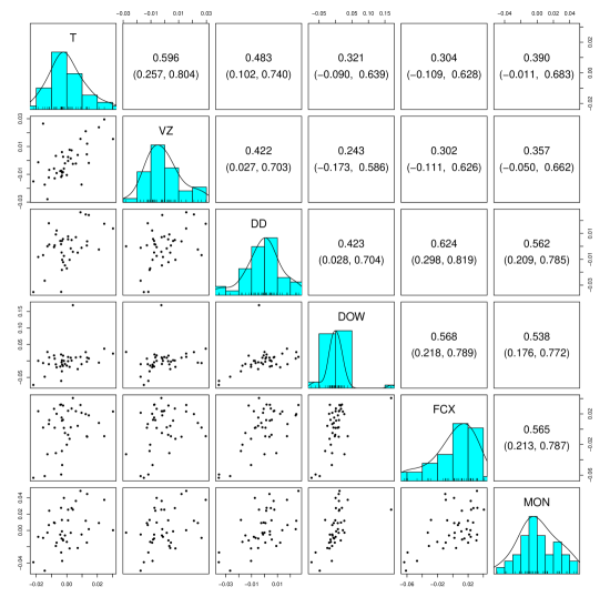
Figure 1: Univariate histograms (on the diagonal), bivariate scatter plots (below the diagonal), and the lag-zero Pearson correlation coefficients with 99% confidence intervals (above the diagonal) for the forty observations of daily log returns of six stocks: “AT&T Inc [T]”, “Verizon Communications [VZ],” “Du Pont (E.I.) [DD],” “Dow Chemical [DOW],” “Freeport-McMoran Cp & Gld [FCX],” and “Monsanto Co. [MON].”

The S&P 100 stocks are classified into ten sectors by Global Industry Classification Standard (GICS). To illustrate the advantages of the proposed tests, we focus on detecting dependence between two such sectors: (1) Telecommunications, including “AT&T Inc [T]” and “Verizon Communications [VZ]” stocks; and (2) Materials, including “Du Pont (E.I.) [DD]”, “Dow Chemical [DOW]”, “Freeport-McMoran Cp & Gld [FCX]”, and “Monsanto Co. [MON]” stocks.

Figure 1 presents univariate histograms and bivariate scatterplots for the forty observations (separated by three months) of the daily log returns of the six stocks mentioned above. We notice that all univariate marginals are skewed and/or heavy-tailed. We also notice that the lag-zero Pearson correlations between any stock in {T, VZ} and any stock in {DD, DOW, FCX, MON} are relatively small, and that most correlations are non-significant at significance level $1\%$.

We applied the four rank-based tests (quadrant (sign), Spearman, Kendall, van der Waerden) proposed in Section 3.3 to the forty bivariate observations of (T, VZ) and either (DD, DOW), (DD, FCX), (DD, MON), (DOW, FCX), (DOW, MON), or (FCX, MON). These tests are based on the matrices defined in (5)– ​(8). As a benchmark, we also include Wilks’ Gaussian likelihood ratio test (LRT). The $p$-values for all these tests are reported in Table 1. One observes that the rank-based tests perform as well as Wilks’ LRT in the first three columns while, in the last three, they yield strong evidence against independence whereas Wilks is unable to reject independence at 5% significance level. The case of Telecommunications and Materials is particularly clear, with $p$-values of 0.006 for van der Waerden and 0.007 for Spearman in testing independence between (T,VZ) and (DOW, FCX)—to be compared with Wilks’ $p$-value 0.174.

Table 1: P-values of the quadrant, Spearman, Kendall, van der Waerden, and Wilks tests of the hypotheses of independence between the bivariate vector (T,VZ) and each of the six bivariate vectors (DD, DOW), (DD, FCX), (DD, MON), (DOW, FCX), (DOW, MON), or (FCX, MON).

		(DD, DOW)	(DD, FCX)	(DD, MON)	(DOW, FCX)	(DOW, MON)	(FCX, MON)
quadrant (sign)		$0.002$	$0.050$	$0.027$	$0.013$	$0.008$	$0.023$
Spearman		$\!\!\!\!\!\!<0.001$	$0.005$	$0.004$	$0.007$	$0.001$	$0.011$
Kendall	(T,VZ)	$0.002$	$0.013$	$0.016$	$0.011$	$0.002$	$0.036$
van der Waerden		$\!\!\!\!\!\!<0.001$	$0.012$	$0.011$	$0.006$	$\!\!\!\!\!\!<0.001$	$0.010$
Wilks (LRT)		$0.011$	$0.016$	$0.009$	$0.174$	$0.072$	$0.074$

Rank-based sign, Spearman, Kendall, and van der Waerden tests, thus, are able to detect dependencies that Wilks’ traditional pseudo-Gaussian test cannot.

1.4 Outline of the paper

The paper is organized as follows. Section 2 briefly reviews the notions of center-outward ranks and signs. Section 3 introduces our rank tests of multivariate independence. In Section 4, we establish a Chernoff–Savage property and a Hodges–Lehmann result for our center-outward van der Waerden and Spearman tests, respectively. We briefly conclude in Section 5. Due to the importance, all the proofs are given in Section 6. The auxiliary results and numerical experiments are deferred to the supplement (Shi et al., 2024).

2 Center-outward distribution functions, ranks, and signs

2.1 Definitions

Denoting by ${\mathbb{S}_{d}}$ and ${\mathcal{S}_{d-1}}$, respectively, the open unit ball and the unit hypersphere in ${\mathbb{R}}^{d}$, let ${\rm U}_{d}$ stand for the spherical uniform distribution over ${\mathbb{S}_{d}}$. Let ${\cal P}_{d}$ denote the class of Lebesgue-absolutely continuous distributions over $\mathbbm{R}^{d}$. For any ${\rm P}$ in ${\cal P}_{d}$, the main result in McCann (1995) then implies the existence of a ${\rm P}$-a.s. unique gradient $\nabla\phi$ of a convex (and lower semi-continuous) function $\phi:\mathbbm{R}^{d}\to\mathbbm{R}$ such that $\nabla\phi$ pushes $\mathrm{P}$ forward to ${\rm U}_{d}$, i.e., $\nabla\phi({\bf Z})\sim{\rm U}_{d}$ under ${\bf Z}\sim\mathrm{P}$. Call center-outward distribution function of $\rm P$ any version ${\bf F}_{\scriptscriptstyle\pm}$ of this a.e. unique gradient.

Turning to sample versions, denote by $\mathbf{Z}^{(n)}\!\coloneqq\big{(}\mathbf{Z}_{1}^{(n)},\dots,\mathbf{Z}_{n}^{(n)}\big{)}$, $n\in~{}\!\mathbb{N}$ a triangular array of i.i.d. $d$-dimensional random vectors with distribution $\mathrm{P}$. The empirical center-outward distribution function ${\bf F}_{\scriptscriptstyle\pm}^{(n)}$ of $\mathbf{Z}^{(n)}$ maps the $n$-tuple $\mathbf{Z}_{1}^{(n)},\dots,\mathbf{Z}_{n}^{(n)}$ to a “regular” grid $\mathfrak{G}_{n}$ of the unit ball ${\mathbb{S}}_{d}$.

This regular grid $\mathfrak{G}_{n}$ is expected to approximate the spherical uniform distribution ${\rm U}_{d}$ over the unit ball ${\mathbb{S}_{d}}$. The only mathematical requirement needed for the asymptotic results below is the weak convergence, as $n\to\infty$, of the uniform discrete distribution over $\mathfrak{G}_{n}$ to the spherical uniform distribution ${\rm U}_{d}$. A spherical uniform i.i.d. sample of $n$ points over ${\mathbb{S}_{d}}$ (almost surely) satisfies such a requirement. Since the spherical uniform is highly symmetric, further symmetries can be imposed on $\mathfrak{G}_{n}$, though, which only can improve the convergence to ${\rm U}_{d}$. In the sequel, we throughout assume that the grids $\mathfrak{G}_{n}$ are symmetric with respect to the origin, i.e., ${\bf u}\in\mathfrak{G}_{n}$ implies ${-\bf u}\in\mathfrak{G}_{n}$, which considerably simplifies formulas. More symmetry, however, can be assumed: see Section 2.2 below. It should be insisted, however, that imposing such symmetry assumptions does not restrict the generality of the results since the construction of the grid is entirely under control.

The empirical counterpart ${\bf F}_{\scriptscriptstyle\pm}^{(n)}$ of ${\bf F}_{\scriptscriptstyle\pm}$ is defined as the bijective mapping from $\mathbf{Z}_{1}^{(n)},\dots,\mathbf{Z}_{n}^{(n)}$ to the grid $\mathfrak{G}_{n}$ that minimizes $\sum_{i=1}^{n}\big{\|}{\bf F}_{\scriptscriptstyle\pm}^{(n)}(\mathbf{Z}_{i}^{(n)})-\mathbf{Z}_{i}^{(n)}\big{\|}^{2}$, where $\|\cdot\|$ denotes the Euclidean norm. That mapping is unique with probability one; in practice, it is obtained via a simple optimal assignment (pairing) algorithm—a linear program; see Shi, Drton, and Han (2022, Section 5.1) for a review and references therein. Call rescaled center-outward rank of $\mathbf{Z}_{i}^{(n)}$ the modulus

$$\widetilde{R}^{(n)}_{i;{{{\scriptscriptstyle\pm}}}}\coloneqq\big{\|}{\bf F}_{\scriptscriptstyle\pm}^{(n)}(\mathbf{Z}_{i}^{(n)})\big{\|},\quad i=1,\ldots,n$$ (1)

and center-outward sign of $\mathbf{Z}_{i}^{(n)}$ the unit vector

$${\bf S}^{(n)}_{i;{{\scriptscriptstyle\pm}}}\coloneqq{\bf F}_{\scriptscriptstyle\pm}^{(n)}(\mathbf{Z}_{i}^{(n)})\big{/}\big{\|}{\bf F}_{\scriptscriptstyle\pm}^{(n)}(\mathbf{Z}_{i}^{(n)})\big{\|}\quad\text{for ${\bf F}_{\scriptscriptstyle\pm}^{(n)}(\mathbf{Z}_{i}^{(n)})\neq{\bf 0}$;}$$ (2)

put ${\bf S}^{(n)}_{i;{{{\scriptscriptstyle\pm}}}}={\bf 0}$ for ${\bf F}_{\scriptscriptstyle\pm}^{(n)}(\mathbf{Z}_{i}^{(n)})={\bf 0}$. When the grid $\mathfrak{G}_{n}$ is obtained, as in Section 2.2 below, with a factorization of $n$ into $n_{R}n_{S}+n_{0}$, call $R^{(n)}_{i;{{{\scriptscriptstyle\pm}}}}\coloneqq(n_{R}+1)\widetilde{R}^{(n)}_{i;{{{\scriptscriptstyle\pm}}}}$, which takes values $(0),1,\ldots,n_{R}$, the center-outward rank of $\mathbf{Z}_{i}^{(n)}$.

2.2 Grid selection

The way (rescaled) ranks and signs in (1) and (2) are constructed, thus, depends on the way the grid $\mathfrak{G}_{n}$ is selected. As already mentioned, the only requirement for asymptotic results (as in Proposition 2.3 below) is the weak convergence to the spherical uniform ${\rm U}_{d}$ of the empirical distribution, ${\rm U}^{(n)}_{\mathfrak{G}}$, say, over $\mathfrak{G}_{n}$. The closer ${\rm U}^{(n)}_{\mathfrak{G}}$ to ${\rm U}_{d}$, the better. Imposing on $\mathfrak{G}_{n}$ some of the many symmetries of ${\rm U}_{d}$ only can improve the finite-sample performance of ${\rm U}^{(n)}_{\mathfrak{G}}$ as an approximation of ${\rm U}_{d}$. Since ${\rm U}_{d}$ is the product of a uniform over the distances to the origin and a uniform over the unit sphere ${\cal S}_{d-1}$, it is natural to select $\mathfrak{G}_{n}$ such that ${\rm U}^{(n)}_{\mathfrak{G}}$ similarly factorizes. This can be obtained as follows:

1. first factorize $n$ into $n=n_{R}n_{S}+n_{0}$, with $0\leq n_{0}<\min(n_{R},n_{S})$ and $\min(n_{R},n_{S})\to\infty$ as $n\to\infty$;

2. next consider a “regular array” $\mathfrak{S}_{n_{S}}\coloneqq\{{\bf s}^{n_{S}}_{1},\ldots,{\bf s}^{n_{S}}_{n_{S}}\}$ of $n_{S}$ points on the sphere ${\cal S}_{d-1}$ (see Remark 2.1 below);

3. construct the grid $\mathfrak{G}_{n}$ consisting in the collection of the $n_{R}n_{S}$ gridpoints of the form

   $$\big{(}r/\big{(}n_{R}+1\big{)}\big{)}{\bf s}^{n_{S}}_{s},\quad r=1,\ldots,n_{R},~{}s=1,\ldots,n_{S},$$

   along with ($n_{0}$ copies of) the origin in case $n_{0}\neq 0$: in total $n-(n_{0}-1)$ or $n$ distinct points, thus, according as $n_{0}>0$ or $n_{0}=0$.

Remark 2.1.

By “regular” array $\mathfrak{S}_{n_{S}}$ over ${\cal S}_{d-1}$ in (b) above, we mean “as regular as possible” an array $\mathfrak{S}_{n_{S}}$—in the sense, for example, of the low-discrepancy sequences of the type considered in numerical integration, Monte-Carlo methods, and experimental design. The asymptotic results in Proposition 2.3 below only require the weak convergence, as $n_{S}\to\infty$, of the uniform discrete distribution over $\mathfrak{S}_{n_{S}}$ to the uniform distribution over ${\cal S}_{d-1}$. A uniform i.i.d. sample of points over ${\cal S}_{d-1}$ (almost surely) satisfies that requirement. However, one can easily construct arrays that are “more regular” than an i.i.d. one. In particular, in order for the grid $\mathfrak{G}_{n}$ described in (a)–(c) above to be symmetric with respect to the origin, one could select an even value of $n_{S}$ and see that ${\bf s}^{n_{S}}_{s}\in\mathfrak{S}_{n_{S}}$ implies $-\,{\bf s}^{n_{S}}_{s}\in\mathfrak{S}_{n_{S}}$, so that $\sum_{i=1}^{n}{\bf S}^{(n)}_{i;{{{\scriptscriptstyle\pm}}}}=n_{R}\sum_{s=1}^{n_{S}}{\bf s}^{n_{S}}_{s}=\boldsymbol{0}$.

Remark 2.2.

Some desirable finite-sample properties, such as strict independence between the ranks and the signs, hold with grids constructed as in (a)–(c) above provided, however, that $n_{0}=0$ or 1. This is due to the fact that the mapping from the sample to the grid is no longer injective for $n_{0}\geq~{}\!2$. This fact, which has no asymptotic consequences (since the number $n_{0}$ of tied values involved is $o(n)$ as $n\to\infty$), is easily taken care of by performing the following tie-breaking device in step (c) of the construction of $\mathfrak{G}_{n}$: (i) randomly select $n_{0}$ directions ${\bf s}^{0}_{1},\ldots,{\bf s}^{0}_{n_{0}}$ in $\mathfrak{S}_{n_{S}}$, then (ii) replace the $n_{0}$ copies of the origin with the new gridpoints $[1/2(n_{R}+1)]{\bf s}^{0}_{1},\ldots,[1/2(n_{R}+1)]{\bf s}^{0}_{n_{0}}.$ This new grid (for simplicity, the same notation ${\mathfrak{G}}_{n}$ is used as for the original one) no longer has multiple points: the optimal pairing between the sample and the grid is bijective and the resulting (rescaled) ranks and signs are mutually independent.

2.3 Main properties

This section summarizes some of the main properties of the concepts defined in Section 2.1; further properties and the proofs can be found in Hallin et al. (2021), Hallin, Hlubinka, and Hudecová (2023), and Hallin (2022). In the following propositions, the grids $\mathfrak{G}_{n}$ used in the construction of the empirical center-outward distribution function ${\bf F}^{(n)}_{{\scriptscriptstyle\pm}}$ are only required to satisfy the minimal assumption of an empirical distribution ${\rm U}^{(n)}_{\mathfrak{G}}$ converging weakly to ${\rm U}_{d}$.

Proposition 2.3.

Let ${\bf F}_{{\scriptscriptstyle\pm}}$ denote the center-outward distribution function of ${\rm P}\in{\cal P}_{d}$. Then,

1. ${\bf F}_{{\scriptscriptstyle\pm}}$ is a probability integral transformation of $\mathbbm{R}^{d}$, that is, ${\bf F}_{{\scriptscriptstyle\pm}}({\bf Z})\sim{\rm U}_{d}$ if and only if ${\bf Z}\sim{\rm P}$; under ${\bf Z}\sim{\rm P}$, $\|{\bf F}_{{\scriptscriptstyle\pm}}({\bf Z})\|$ is uniform over $[0,1)$, ${\bf F}_{{\scriptscriptstyle\pm}}({\bf Z})/\|{\bf F}_{{\scriptscriptstyle\pm}}({\bf Z})\|$ is uniform over the sphere ${\cal S}_{d-1}$, and they are mutually independent.

Let ${\bf Z}^{(n)}_{1},\ldots,{\bf Z}^{(n)}_{n}$ be i.i.d. with distribution ${\rm P}\in{\mathcal{P}}_{d}$ and empirical center-outward distribution function ${\bf F}_{\scriptscriptstyle\pm}^{(n)}$. Then, if there are no ties in the grid $\mathfrak{G}_{n}$,

1. $\big{(}{\bf F}^{(n)}_{{\scriptscriptstyle\pm}}({\bf Z}^{(n)}_{1}),\ldots,{\bf F}^{(n)}_{{\scriptscriptstyle\pm}}({\bf Z}^{(n)}_{n})\big{)}$ is uniformly distributed over the $n!$ permutations of $\mathfrak{G}_{n}$;

2. the $n$-tuple $\big{(}{\bf F}^{(n)}_{{\scriptscriptstyle\pm}}({\bf Z}^{(n)}_{1}),\ldots,{\bf F}^{(n)}_{{\scriptscriptstyle\pm}}({\bf Z}^{(n)}_{n})\big{)}$ is strongly essentially maximal ancillary;

3. (pointwise convergence) for any $i=1,\ldots,n$,

   $${}\Big{\|}{\bf F}^{(n)}_{{\scriptscriptstyle\pm}}({\bf Z}^{(n)}_{i})-{\bf F}_{{\scriptscriptstyle\pm}}({\bf Z}^{(n)}_{i})\Big{\|}\rightarrow 0~{}\textrm{\em a.s.}\quad\text{as}~{}n\to\infty.$$

Assume, moreover, that ${\rm P}$ is in the so-called class ${\cal P}^{+}_{d}\subset{\cal P}_{d}$ of distributions with nonvanishing densities—namely, the class of distributions with density $f\coloneqq{\rm dP}/{\rm d}\mu_{d}$ ($\mu_{d}$ the $d$-dimensional Lebesgue measure) such that, for all $D\in\mathbbm{R}^{+}$, there exist constants $\lambda^{-}_{D;\mathrm{P}}$ and $\lambda^{+}_{D;\mathrm{P}}$ satisfying

$$0<\lambda^{-}_{D;\mathrm{P}}\leq f({\bf z})\leq\lambda^{+}_{D;\mathrm{P}}<\infty$$ (3)

for all $\bf z$ with $\|{\bf z}\|\leq D$. Then,

1. there exists a version of ${\bf F}_{\scriptscriptstyle\pm}$ defining a homeomorphism between the punctured unit ball ${\mathbb{S}}_{d}\!\setminus~{}\!\{{\bf 0}\}$ and $\mathbbm{R}^{d}\setminus{\bf F}_{\scriptscriptstyle\pm}^{-1}(\{{\bf 0}\})$; that version has a continuous inverse ${\bf Q}_{\scriptscriptstyle\pm}$ (with domain ${\mathbb{S}}_{d}\!\setminus\!\{{\bf 0}\}$), which naturally qualifies as ${\rm P}$’s center-outward quantile function;

2. (Glivenko–Cantelli)

   $${\max_{1\leq i\leq n}}\Big{\|}{\bf F}^{(n)}_{{\scriptscriptstyle\pm}}({\bf Z}^{(n)}_{i})-{\bf F}_{{\scriptscriptstyle\pm}}({\bf Z}^{(n)}_{i})\Big{\|}\longrightarrow 0\ \textrm{\em a.s.}\quad\text{as}~{}n\to\infty.$$

Results (v) and (vi) are due to Figalli (2018), Hallin (2017), del Barrio et al. (2018), Hallin et al. (2021) and can be extended (del Barrio, González-Sanz, and Hallin, 2020) to a more general class ${\cal P}_{d}^{\rm conv}$ of absolutely continuous distributions, with density $f$ supported on a open convex set of $\mathbbm{R}^{d}$ but not necessarily the whole space, while the definition of ${\bf F}_{\scriptscriptstyle\pm}$ given in Hallin et al. (2021) aims at selecting, for each ${\rm P}\in{\cal P}_{d}$, a version of $\nabla\phi$ which, whenever ${\rm P}\in{\cal P}_{d}^{\rm conv}$, is yielding the homeomorphism mentioned in (v). For the sake of simplicity, since we are not interested in quantiles, we stick here to the ${\rm P}$-a.s. unique definition given above for ${\rm P}\in{\cal P}_{d}$.

Center-outward distribution functions, ranks, and signs also inherit, from the invariance of squared Euclidean distances, elementary but quite remarkable invariance and equivariance properties under shifts, orthogonal transformations, and global rescaling (see Hallin, Hlubinka, and Hudecová (2023)). Denote by ${\bf F}^{{\bf Z}}_{{\scriptscriptstyle\pm}}$ the center-outward distribution function of $\bf Z$ and by ${\bf F}^{{\bf Z};\mathfrak{G}_{n}}_{{\scriptscriptstyle\pm}}$ the empirical center-outward distribution function of an i.i.d. sample ${\bf Z}_{1},\ldots,{\bf Z}_{n}$ associated with a grid $\mathfrak{G}_{n}$.

Proposition 2.4.

Let $\boldsymbol{\mu}\in\mathbbm{R}^{d}$, $k\in\mathbbm{R}^{+}$, and denote by ${\bf O}$ a $d\times d$ orthogonal matrix. Then,

1. ${\bf F}^{\boldsymbol{\mu}+k{\bf O}{\bf Z}}_{{\scriptscriptstyle\pm}}(\boldsymbol{\mu}+{\bf O}{\bf z})={\bf O}{\bf F}^{\bf Z}_{{\scriptscriptstyle\pm}}({\bf z})$, ${\bf z}\in\mathbbm{R}^{d}$;

2. denoting by ${\bf F}^{\boldsymbol{\mu}+k{\bf O}{\bf Z};{\bf O}\mathfrak{G}_{n}}_{{\scriptscriptstyle\pm}}$ the empirical center-outward distribution function computed from the sample $\boldsymbol{\mu}+k{\bf O}{\bf Z}_{1},\ldots,\boldsymbol{\mu}+k{\bf O}{\bf Z}_{n}$ and the grid ${\bf O}\mathfrak{G}_{n}\coloneqq\{{\bf O}{\bf u}:{\bf u}\in\mathfrak{G}_{n}\}$,

   $${\bf F}^{\boldsymbol{\mu}+k{\bf O}{\bf Z};{\bf O}\mathfrak{G}_{n}}_{{\scriptscriptstyle\pm}}(\boldsymbol{\mu}+k{\bf O}{\bf Z}_{i})={\bf O}{\bf F}^{{\bf Z};\mathfrak{G}_{n}}_{{\scriptscriptstyle\pm}}({\bf Z}_{i}),\quad i=1,\ldots,n.$$ (4)

Note that the orthogonal transformations in Proposition 2.4 include the permutations of $\bf Z$’s components. Invariance with respect to such permutations is an essential requirement for hypothesis testing in multivariate analysis.

3 Rank-based tests for multivariate independence

3.1 Center-outward test statistics for multivariate independence

In this section, we describe the test statistics we are proposing for testing independence between two random vectors. Consider a sample $({\mathbf{X}}^{\prime}_{11},{\mathbf{X}}^{\prime}_{21})^{\prime},({\mathbf{X}}^{\prime}_{12},{\mathbf{X}}^{\prime}_{22})^{\prime},\ldots,({\mathbf{X}}^{\prime}_{1n},{\mathbf{X}}^{\prime}_{2n})^{\prime}$ of $n$ i.i.d. copies of some $(d_{1}+d_{2})\!=\!d$-dimensional random vector $({\mathbf{X}}^{\prime}_{1},{\mathbf{X}}^{\prime}_{2})^{\prime}$ with Lebesgue-absolutely continuous joint distribution ${\rm P}\in{\cal P}_{d}$ and density $f$. We are interested in the null hypothesis under which ${\mathbf{X}}_{1}$ and ${\mathbf{X}}_{2}$, with unspecified marginal distributions ${\rm P}_{1}\in{\cal P}_{d_{1}}$ (density $f_{1}$) and ${\rm P}_{2}\in{\cal P}_{d_{2}}$ (density $f_{2}$), respectively, are mutually independent: $f$ then factorizes into $f=f_{1}f_{2}$.

For $k=1,2$ and $i=1,2,\ldots,n$, denote by $R^{(n)}_{ki;{\scriptscriptstyle\pm}}$, $\widetilde{R}^{(n)}_{ki;{\scriptscriptstyle\pm}}$, and ${\bf S}^{(n)}_{ki;{\scriptscriptstyle\pm}}$ the center-outward rank, rescaled rank, and sign of ${\mathbf{X}}_{ki}$ computed from ${\mathbf{X}}_{k1},{\mathbf{X}}_{k2},\ldots,{\mathbf{X}}_{kn}$ and the grid $\mathfrak{G}_{n}$. Recall that we throughout assume that if ${\bf u}\in\mathfrak{G}_{n}$ then ${-\bf u}\in\mathfrak{G}_{n}$. This implies that $\sum_{i=1}^{n}{\bf S}^{(n)}_{ki;{\scriptscriptstyle\pm}}={\bf 0}$ and $\sum_{i=1}^{n}J_{k}\big{(}\widetilde{R}^{(n)}_{ki;{\scriptscriptstyle\pm}}\big{)}{\bf S}^{(n)}_{ki;{\scriptscriptstyle\pm}}={\bf 0}$ for any score function $J_{k}:[0,1)\to\mathbbm{R}$, $k=1,2$.

Consider now the $d_{1}\times d_{2}$ matrices

$${\stackunder[1pt]{\mathbf{W}}{\scriptscriptstyle\thicksim}}\,\!_{\text{\tiny\rm sign}}^{(n)} \coloneqq\frac{1}{n}\sum_{i=1}^{n}{\bf S}^{(n)}_{1i;{\scriptscriptstyle\pm}}{\bf S}^{(n)\prime}_{2i;{\scriptscriptstyle\pm}},$$ (5)

$${\stackunder[1pt]{\mathbf{W}}{\scriptscriptstyle\thicksim}}\,\!_{\text{\tiny\rm Spearman}}^{(n)} \coloneqq\frac{1}{n}\sum_{i=1}^{n}\widetilde{R}^{(n)}_{1i;{\scriptscriptstyle\pm}}\widetilde{R}^{(n)}_{2i;{\scriptscriptstyle\pm}}{\bf S}^{(n)}_{1i;{\scriptscriptstyle\pm}}{\bf S}^{(n)\prime}_{2i;{\scriptscriptstyle\pm}},$$ (6)

$${\stackunder[1pt]{\mathbf{W}}{\scriptscriptstyle\thicksim}}\,\!_{\text{\tiny\rm Kendall}}^{(n)} \coloneqq{n\choose 2}^{-1}\sum_{i<i^{\prime}}\text{sign}\Big{[}\Big{(}\widetilde{R}^{(n)}_{1i;{\scriptscriptstyle\pm}}{\bf S}^{(n)}_{1i;{\scriptscriptstyle\pm}}-\widetilde{R}^{(n)}_{1i^{\prime};{\scriptscriptstyle\pm}}{\bf S}^{(n)}_{1i^{\prime};{\scriptscriptstyle\pm}}\Big{)}\Big{(}\widetilde{R}^{(n)}_{2i;{\scriptscriptstyle\pm}}{\bf S}^{(n)}_{2i;{\scriptscriptstyle\pm}}-\widetilde{R}^{(n)}_{2i^{\prime};{\scriptscriptstyle\pm}}{\bf S}^{(n)}_{2i^{\prime};{\scriptscriptstyle\pm}}\Big{)}^{\prime}\Big{]},$$ (7)

where sign$\big{[}{\bf M}\big{]}$ stands for the matrix collecting the signs of the entries of a real matrix $\bf M$. More generally, let

$${\stackunder[1pt]{\mathbf{W}}{\scriptscriptstyle\thicksim}}\,\!_{J}^{(n)} \coloneqq\frac{1}{n}\sum_{i=1}^{n}J_{1}\Big{(}{\widetilde{R}^{(n)}_{1i;{\scriptscriptstyle\pm}}}\Big{)}J_{2}\Big{(}{\widetilde{R}^{(n)}_{2i;{\scriptscriptstyle\pm}}}\Big{)}{\bf S}^{(n)}_{1i;{\scriptscriptstyle\pm}}{\bf S}^{(n)\prime}_{2i;{\scriptscriptstyle\pm}},$$ (8)

where the score functions $J_{k}:[0,1)\to\mathbbm{R}$, $k=1,2$ are continuous and square-integrable, with

$$0<\lim_{n\to\infty}n^{-1}\sum_{i=1}^{n}J_{k}^{2}(r_{i})=\int_{0}^{1}J_{k}^{2}(u){\rm d}u\eqqcolon\sigma_{J_{k}}^{2}<\infty$$ (9)

for any $\{r_{1},\dots,r_{n}\}$ such that the uniform distribution over which converges weakly to the uniform distribution over $[0,1]$. This assumption on score functions will be made throughout the remainder of the paper. The matrices defined in (5)–(8) clearly constitute matrices of cross-covariance measurements based on center-outward ranks and signs (for ${\stackunder[1pt]{\mathbf{W}}{\scriptscriptstyle\thicksim}}\,\!_{\text{\tiny\rm sign}}^{(n)}$, signs only). For $d_{1}=1=d_{2}$, it is easily seen that ${\stackunder[1pt]{\mathbf{W}}{\scriptscriptstyle\thicksim}}\,\!_{\text{\tiny\rm sign}}^{(n)}$, ${\stackunder[1pt]{\mathbf{W}}{\scriptscriptstyle\thicksim}}\,\!_{\text{\tiny\rm Spearman}}^{(n)}$, and ${\stackunder[1pt]{\mathbf{W}}{\scriptscriptstyle\thicksim}}\,\!_{\text{\tiny\rm Kendall}}^{(n)}$, up to scaling constants, reduce to the classical quadrant, Spearman, and Kendall test statistics, while ${\stackunder[1pt]{\mathbf{W}}{\scriptscriptstyle\thicksim}}\,\!_{J}^{(n)}$ yields a matrix-valued score-based extension of Spearman’s correlation coefficient.

3.2 Asymptotic representation and asymptotic normality

Clearly, neither the ranks nor the signs are mutually independent ($n-1$ rank and sign pairs indeed determine the last pair): traditional central-limit theorems thus do not apply. However, as we show now, each of the rank-based matrices defined in (5)–(8) admits an asymptotic representation in terms of i.i.d. variables. More precisely, defining ${\bf S}_{ki;{\scriptscriptstyle\pm}}$ as ${\bf F}_{k;{\scriptscriptstyle\pm}}({\bf X}_{ki})\big{/}\big{\|}{\bf F}_{k;{\scriptscriptstyle\pm}}({\bf X}_{ki})\big{\|}$ if ${\bf F}_{k;{\scriptscriptstyle\pm}}({\bf X}_{ki})\neq{\bf 0}$ and ${\bf 0}$ otherwise for $k=1,2$, let

$${{\mathbf{W}}}\,\!_{\text{\tiny\rm sign}}^{(n)} \coloneqq\frac{1}{n}\sum_{i=1}^{n}{\bf S}_{1i;{\scriptscriptstyle\pm}}{\bf S}^{\prime}_{2i;{\scriptscriptstyle\pm}},$$ (10)

$${{\mathbf{W}}}\,\!_{\text{\tiny\rm Spearman}}^{(n)} \coloneqq\frac{1}{n}\sum_{i=1}^{n}{\bf F}_{1;{\scriptscriptstyle\pm}}({\bf X}_{1i}){\bf F}^{\prime}_{2;{\scriptscriptstyle\pm}}({\bf X}_{2i}),$$ (11)

$${{\mathbf{W}}}\,\!_{\text{\tiny\rm Kendall}}^{(n)} \coloneqq{n\choose 2}^{-1}\sum_{i<i^{\prime}}\text{sign}\Big{[}\Big{(}{\bf F}_{1;{\scriptscriptstyle\pm}}({\bf X}_{1i})-{\bf F}_{1;{\scriptscriptstyle\pm}}({\bf X}_{1i^{\prime}})\Big{)}\Big{(}{\bf F}_{2;{\scriptscriptstyle\pm}}({\bf X}_{2i})-{\bf F}_{2;{\scriptscriptstyle\pm}}({\bf X}_{2i^{\prime}})\Big{)}^{\prime}\,\Big{]},$$ (12)

and

$$\qquad{{\mathbf{W}}}\,\!_{J}^{(n)}\coloneqq\frac{1}{n}\sum_{i=1}^{n}J_{1}\Big{(}\big{\|}{\bf F}_{1;{\scriptscriptstyle\pm}}({\bf X}_{1i})\big{\|}\Big{)}J_{2}\Big{(}\big{\|}{\bf F}_{2;{\scriptscriptstyle\pm}}({\bf X}_{2i})\big{\|}\Big{)}{\bf S}_{1i;{\scriptscriptstyle\pm}}{\bf S}^{\prime}_{2i;{\scriptscriptstyle\pm}}.$$ (13)

The following asymptotic representation results then hold under the null hypothesis of independence (hence, also under contiguous alternatives). As usual, let $\text{\rm vec}({\mathbf{A}})\coloneqq({\mathbf{a}}_{1}^{\prime},\dots,{\mathbf{a}}_{m}^{\prime})^{\prime}$ for an $n\times~{}\!m$ matrix ${\mathbf{A}}=({\mathbf{a}}_{1},\dots,{\mathbf{a}}_{m})$ and write ${\bf X}^{(n)}=o_{\text{\rm q.m.}}(c^{(n)})$ when, for some sequence $c^{(n)}$ of positive real numbers, $|X^{(n)}_{j}|\leq Y^{(n)}c^{(n)}$ for each component $X^{(n)}_{j}$ of ${\bf X}^{(n)}$, with $\lim_{n\to\infty}\mathrm{E}[(Y^{(n)})^{2}]=0$.

Lemma 3.1.

Under the null hypothesis of independence, as $n$ tends to infinity, $\text{\rm vec}\big{(}{\stackunder[1pt]{\mathbf{W}}{\scriptscriptstyle\thicksim}}\,\!_{\text{\tiny\rm sign}}^{(n)}\!-{{\mathbf{W}}}\,\!_{\text{\tiny\rm sign}}^{(n)}\big{)}$, $\text{\rm vec}\big{(}{\stackunder[1pt]{\mathbf{W}}{\scriptscriptstyle\thicksim}}\,\!_{\text{\tiny\rm Spearman}}^{(n)}\!-{{\mathbf{W}}}\,\!_{\text{\tiny\rm Spearman}}^{(n)}\big{)}$, $\text{\rm vec}\big{(}{\stackunder[1pt]{\mathbf{W}}{\scriptscriptstyle\thicksim}}\,\!_{\text{\tiny\rm Kendall}}^{(n)}\!-{{\mathbf{W}}}\,\!_{\text{\tiny\rm Kendall}}^{(n)}\big{)}$, and $\text{\rm vec}\big{(}{\stackunder[1pt]{\mathbf{W}}{\scriptscriptstyle\thicksim}}\,\!_{J}^{(n)}-{{\mathbf{W}}}\,\!_{J}^{(n)}\big{)}$ allare $\,o_{\text{\rm q.m.}}(n^{-1/2})$.

The asymptotic normality of vec$({\stackunder[1pt]{\mathbf{W}}{\scriptscriptstyle\thicksim}}\,\!_{\text{\tiny\rm sign}}^{(n)})$, vec$({\stackunder[1pt]{\mathbf{W}}{\scriptscriptstyle\thicksim}}\,\!_{\text{\tiny\rm Spearman}}^{(n)})$, vec$({\stackunder[1pt]{\mathbf{W}}{\scriptscriptstyle\thicksim}}\,\!_{\text{\tiny\rm Kendall}}^{(n)})$, and vec$({\stackunder[1pt]{\mathbf{W}}{\scriptscriptstyle\thicksim}}\,\!_{J}^{(n)})$ follows immediately from the asymptotic representation results and the standard central-limit behavior of vec$({{\mathbf{W}}}\,\!_{\text{\tiny\rm sign}}^{(n)})$, vec$({{\mathbf{W}}}\,\!_{\text{\tiny\rm Spearman}}^{(n)})$, vec$({{\mathbf{W}}}\,\!_{\text{\tiny\rm Kendall}}^{(n)})$, and vec$({{\mathbf{W}}}\,\!_{J}^{(n)})$.

Proposition 3.2.

Under the null hypothesis of independence, as $n$ tends to infinity, $n^{1/2}{\rm vec}({\stackunder[1pt]{\mathbf{W}}{\scriptscriptstyle\thicksim}}\,\!_{\text{\tiny\rm sign}}^{(n)}),$ $n^{1/2}{\rm vec}({\stackunder[1pt]{\mathbf{W}}{\scriptscriptstyle\thicksim}}\,\!_{\text{\tiny\rm Spearman}}^{(n)}),$ $n^{1/2}{\rm vec}({\stackunder[1pt]{\mathbf{W}}{\scriptscriptstyle\thicksim}}\,\!_{\text{\tiny\rm Kendall}}^{(n)}),$ and $n^{1/2}{\rm vec}({\stackunder[1pt]{\mathbf{W}}{\scriptscriptstyle\thicksim}}\,\!_{J}^{(n)})$ are asymptotically normal with mean vectors ${\bf 0}_{d_{1}d_{2}}$ and covariance matrices

$$\frac{1}{d_{1}d_{2}}{\bf I}_{d_{1}d_{2}},\quad\frac{1}{9d_{1}d_{2}}{\bf I}_{d_{1}d_{2}},\quad\frac{4}{9}{\bf I}_{d_{1}d_{2}},\quad\text{and}\quad\frac{\sigma^{2}_{J_{1}}\sigma^{2}_{J_{2}}}{d_{1}d_{2}}{\bf I}_{d_{1}d_{2}},\vspace{-1mm}$$

respectively.

3.3 Center-outward sign, Spearman, Kendall, and score tests

Associated with ${\stackunder[1pt]{\mathbf{W}}{\scriptscriptstyle\thicksim}}\,\!_{\text{\tiny\rm sign}}^{(n)}$, ${\stackunder[1pt]{\mathbf{W}}{\scriptscriptstyle\thicksim}}\,\!_{\text{\tiny\rm Spearman}}^{(n)}$, ${\stackunder[1pt]{\mathbf{W}}{\scriptscriptstyle\thicksim}}\,\!_{\text{\tiny\rm Kendall}}^{(n)}$, and ${\stackunder[1pt]{\mathbf{W}}{\scriptscriptstyle\thicksim}}\,\!_{J}^{(n)}$ are the quadrant or sign, Spearman, Kendall, and score test statistics

$${\stackunder[1pt]{T}{\scriptscriptstyle\thicksim}}\,\!_{\text{\tiny\rm sign}}^{(n)} \coloneqq nd_{1}d_{2}\big{\|}{\stackunder[1pt]{\mathbf{W}}{\scriptscriptstyle\thicksim}}\,\!_{\text{\tiny\rm sign}}^{(n)}\big{\|}^{2}_{\mathrm{F}},\quad {\stackunder[1pt]{T}{\scriptscriptstyle\thicksim}}\,\!_{\text{\tiny\rm Spearman}}^{(n)} \coloneqq 9nd_{1}d_{2}\big{\|}{\stackunder[1pt]{\mathbf{W}}{\scriptscriptstyle\thicksim}}\,\!_{\text{\tiny\rm Spearman}}^{(n)}\big{\|}^{2}_{\mathrm{F}},\quad$$

$${\stackunder[1pt]{T}{\scriptscriptstyle\thicksim}}\,\!_{\text{\tiny\rm Kendall}}^{(n)} \coloneqq\frac{9n}{4}\big{\|}{\stackunder[1pt]{\mathbf{W}}{\scriptscriptstyle\thicksim}}\,\!_{\text{\tiny\rm Kendall}}^{(n)}\big{\|}^{2}_{\mathrm{F}},\qquad\qquad\text{and} {\stackunder[1pt]{T}{\scriptscriptstyle\thicksim}}\,\!_{J}^{(n)} \coloneqq\frac{nd_{1}d_{2}}{\sigma^{2}_{J_{1}}\sigma^{2}_{J_{2}}}\big{\|}{\stackunder[1pt]{\mathbf{W}}{\scriptscriptstyle\thicksim}}\,\!_{J}^{(n)}\big{\|}^{2}_{\mathrm{F}},$$

respectively, where $\|{\bf M}\|_{\mathrm{F}}$ denotes the Frobenius norm of a matrix $\bf M$, and $\sigma^{2}_{J_{1}}$, $\sigma^{2}_{J_{2}}$ are defined as in (9). In particular, considering the van der Waerden score functions $J^{\text{\tiny{\rm vdW}}}_{k}(u)\!\coloneqq\!\big{(}F^{-1}_{\chi^{2}_{d_{k}}}\!(u)\big{)}^{\!1/2}\!$, where $F_{\chi^{2}_{d}}$ stands for the $\chi^{2}_{d}$ distribution function, the van der Waerden test statistic is ${\stackunder[1pt]{T}{\scriptscriptstyle\thicksim}}\,\!_{\text{\rm{\tiny vdW}}}^{(n)}=\,\,{\stackunder[1pt]{T}{\scriptscriptstyle\thicksim}}\,\!_{J^{\text{\tiny{\rm vdW}}}}^{(n)}=n\big{\|}{\stackunder[1pt]{\mathbf{W}}{\scriptscriptstyle\thicksim}}\,\!_{J^{\text{\tiny{\rm vdW}}}}^{(n)}\big{\|}^{2}_{\mathrm{F}}$.

In view of the asymptotic normality results in Proposition 3.2, the tests ${\psi}\,\!_{\text{\tiny\rm sign}}^{(n)}$, ${\psi}\,\!_{\text{\tiny\rm Spearman}}^{(n)}$, ${\psi}\,\!_{\text{\tiny\rm Kendall}}^{(n)}$, ${\psi}\,\!_{\text{\tiny\rm vdW}}^{(n)}$, and ${\psi}\,\!_{J}^{(n)}$ rejecting the null hypothesis of independence whenever ${\stackunder[1pt]{T}{\scriptscriptstyle\thicksim}}\,\!_{\text{\tiny\rm sign}}^{(n)}$, ${\stackunder[1pt]{T}{\scriptscriptstyle\thicksim}}\,\!_{\text{\tiny\rm Spearman}}^{(n)}$, ${\stackunder[1pt]{T}{\scriptscriptstyle\thicksim}}\,\!_{\text{\tiny\rm Kendall}}^{(n)}$, ${\stackunder[1pt]{T}{\scriptscriptstyle\thicksim}}\,\!_{\text{\tiny\rm vdW}}^{(n)}$ or ${\stackunder[1pt]{T}{\scriptscriptstyle\thicksim}}\,\!_{J}^{(n)}$, respectively, exceed the $(1-~{}\!\alpha)$-quantile $\chi^{2}_{d_{1}d_{2};1-\alpha}$ of a chi-square distribution with $d_{1}d_{2}$ degrees of freedom have asymptotic level $\alpha$. These tests are, however, strictly distribution-free, and exact critical values can be computed or simulated as well. The tests based on ${\stackunder[1pt]{T}{\scriptscriptstyle\thicksim}}\,\!_{\text{\tiny\rm sign}}^{(n)}$, ${\stackunder[1pt]{T}{\scriptscriptstyle\thicksim}}\,\!_{\text{\tiny\rm Spearman}}^{(n)}$, ${\stackunder[1pt]{T}{\scriptscriptstyle\thicksim}}\,\!_{\text{\tiny\rm Kendall}}^{(n)}$, and ${\stackunder[1pt]{T}{\scriptscriptstyle\thicksim}}\,\!_{\text{\tiny\rm vdW}}^{(n)}$ are multivariate extensions of the traditional quadrant, Spearman, Kendall and van der Waerden tests, respectively, to which they reduce for $d_{1}~{}\!=~{}\!1=~{}\!d_{2}$.

4 Local asymptotic powers

While there is only one way for two random vectors ${\bf X}_{1}$ and ${\bf X}_{2}$ to be independent, their mutual dependence can take many forms. The classical benchmark, in testing for bivariate independence, is a “local” form of an independent component analysis model that goes back to Konijn (1956) and Hájek and Šidák (1967). Multivariate elliptical extensions of such alternatives have been considered also by Gieser and Randles (1997), Taskinen, Kankainen, and Oja (2003), Hallin and Paindaveine (2008), and Oja, Paindaveine, and Taskinen (2016).

4.1 Generalized Konijn families

Let ${\bf X}^{*}=({\bf X}^{*\prime}_{1},{\bf X}^{*\prime}_{2})^{\prime}$, where ${\bf X}^{*}_{1}$ and ${\bf X}^{*}_{2}$ are mutually independent random vectors, with absolutely continuous distributions ${\rm P}_{1}$ over $\mathbbm{R}^{d_{1}}$ and ${\rm P}_{2}$ over $\mathbbm{R}^{d_{2}}$ and densities $f_{1}$ and $f_{2}$, respectively. Then ${\bf X}^{*}$ has density $f=f_{1}f_{2}$ over $\mathbbm{R}^{d}$. Consider

$${\bf X}=\left(\!\begin{array}[]{c}{\bf X}_{1}\\ {\bf X}_{2}\end{array}\!\right)\coloneqq{\bf M}_{\delta}\left(\!\begin{array}[]{c}{\bf X}^{*}_{1}\\ {\bf X}^{*}_{2}\end{array}\!\right)\coloneqq\left(\!\begin{array}[]{cc}(1-{\delta}){\bf I}_{d_{1}}&{\delta}{\bf M_{1}}\\ {\delta}{\bf M}_{2}&(1-{\delta}){\bf I}_{d_{2}}\end{array}\!\right)\!\left(\!\begin{array}[]{c}{\bf X}^{*}_{1}\\ {\bf X}^{*}_{2}\end{array}\!\right)$$ (22)

where ${\delta}\!\in\!\mathbbm{R}$ and ${\bf M}_{1}\!\in\!\mathbbm{R}^{d_{1}\times d_{2}}$, ${\bf M}_{2}\!\in\!\mathbbm{R}^{d_{2}\times d_{1}}$ are nonzero matrices. For given ${\rm P}_{1}$, ${\rm P}_{2}$, ${\bf M}_{1}$, ${\bf M}_{2}$, and $\delta$, the distribution ${\rm P}^{\bf X}_{\delta}({\rm P}_{1},{\rm P}_{2};{\bf M}_{1},{\bf M}_{2})$ of ${\bf X}$ belongs to the one-parameter family

$${\cal P}^{\bf X}_{{\rm P}_{1},{\rm P}_{2};{\bf M}_{1},{\bf M}_{2}}\coloneqq\left\{{\rm P}^{\bf X}_{\delta}({\rm P}_{1},{\rm P}_{2};{\bf M}_{1},{\bf M}_{2})|\,{\delta}\in\mathbbm{R}\right\};$$

call it a generalized Konijn family. Independence between ${\bf X}_{1}$ and ${\bf X}_{2}$, in such families, holds iff $\delta=0$.

Sequences of the form ${\rm P}^{\bf X}_{{n^{-1/2}\tau}}({\rm P}_{1},{\rm P}_{2};{\bf M}_{1},{\bf M}_{2})\vspace{1mm}$ with $\tau\neq 0$, as we shall see, define contiguous alternatives to the null hypothesis of independence in a sample of size $n$. More precisely, consider the following regularity assumptions on ${\rm P}_{1}$ and ${\rm P}_{2}$ (on their densities $f_{1}$ and $f_{2}$).

Assumption 4.1.

(K1) The densities $f_{1}$ and $f_{2}$ are such that

$$\int_{\mathbbm{R}^{d_{k}}}\!{\bf x}f_{k}({\bf x}){\rm d}{\bf x}={\bf 0}\quad\text{and}\quad 0<\int_{\mathbbm{R}^{d_{k}}}\!{\bf x}{\bf x}^{\prime}f_{k}({\bf x}){\rm d}{\bf x}\eqqcolon{\boldsymbol{\Sigma}}_{k}<\infty,\quad k=1,2,$$

where $0<{\boldsymbol{\Sigma}}_{k}<\infty,$ means the covariance matrix ${\boldsymbol{\Sigma}}_{k}$ is finite and positive definite.

1. The functions ${\bf x}_{k}\mapsto(f_{k}({\bf x}_{k}))^{1/2}$, $k=1,2$ admit quadratic mean partial derivatives

   $$D_{\ell}[(f_{k})^{1/2}],\quad\ell=1,\ldots,d_{k},\ k=1,2.\vspace{-1mm}$$

2. The score ${\boldsymbol{\varphi}}\mkern-2.0mu\coloneqq\mkern-2.0mu\left({\boldsymbol{\varphi}}_{1}^{\prime},{\boldsymbol{\varphi}}_{2}^{\prime}\right)^{\prime}\mkern-2.0mu\coloneqq\mkern-2.0mu\left(\varphi_{1;1},\ldots,\varphi_{1;d_{1}},\varphi_{2;1},\ldots,\varphi_{2;d_{2}}\right)^{\prime}$ with $\varphi_{k;\ell}\mkern-2.0mu\coloneqq\mkern-2.0mu-2D_{\ell}[(f_{k})^{1/2}]/(f_{k})^{1/2}$ is such that $0<~{}\int_{{\mathbbm{R}}^{d_{k}}}\big{(}\varphi_{k;\ell}({\bf x})\big{)}^{2}f_{k}({\bf x}){\rm d}{\bf x}<\infty$, $k=1,2$, $\ell=1,\ldots,d_{k}$, and

   $$\mathcal{J}_{k}\coloneqq{\text{\rm Var}}\left({\bf X}^{*\prime}_{k}{\boldsymbol{\varphi}}_{k}({\bf X}^{*}_{k})\right)=\int_{{\mathbbm{R}}^{d_{k}}}\left({\bf x}^{\prime}{\boldsymbol{\varphi}}_{k}({\bf x})-d_{k}\right)^{2}f_{k}({\bf x}){\rm d}{\bf x},\quad k=1,2\vspace{-2mm}$$

   is finite and strictly positive.

It should be stressed that these regularity assumptions are not to be imposed on the observations in order for our rank-based tests to be valid; they only are required for deriving local power and ARE results.

The following local asymptotic normality (LAN) property then holds in the vicinity of ${\delta}=0$.

Lemma 4.2.

Denote by ${\rm P}^{(n)}_{\delta}$​, $n\in\mathbbm{N}$, the distribution of the triangular array ${\bf X}^{(n)}\coloneqq({\bf X}_{1}^{(n)},\ldots,{\bf X}_{n}^{(n)})$ of $n$ independent copies of  ${\bf X}=({\bf X}^{\prime}_{1},{\bf X}_{2}^{\prime})^{\prime}\sim{\rm P}^{\bf X}_{\delta}({\rm P}_{1},{\rm P}_{2};{\bf M}_{1},{\bf M}_{2})\in{\cal P}^{\bf X}_{{\rm P}_{1},{\rm P}_{2};{\bf M}_{1},{\bf M}_{2}}$, where ${\rm P}_{1}$ and ${\rm P}_{2}$ satisfy Assumption 4.1. Then, the family $\big{\{}{\rm P}^{(n)}_{\delta}|\,\delta\in{\mathbb{R}}\big{\}}$ is Locally Asymptotically Normal (LAN) at ${\delta}=~{}\!0$, with root-$n$ contiguity rate, central sequence

$$\Delta^{(n)}({\bf X}^{(n)})\coloneqq n^{-1/2}\sum_{i=1}^{n}\left[{\bf X}^{(n)\prime}_{1i}{\bf M}_{2}^{\prime}{\boldsymbol{\varphi}}_{2}({\bf X}^{(n)}_{2i})\right. +{\bf X}^{(n)\prime}_{2i}{\bf M}_{1}^{\prime}{\boldsymbol{\varphi}}_{1}({\bf X}^{(n)}_{1i})$$

$$\left.-\Big{(}{\bf X}^{(n)\prime}_{1i}{\boldsymbol{\varphi}}_{1}({\bf X}^{(n)}_{1i})-d_{1}\Big{)}-\Big{(}{\bf X}^{(n)\prime}_{2i}{\boldsymbol{\varphi}}_{2}({\bf X}_{2i}^{(n)})-d_{2}\Big{)}\right],$$

and Fisher information

$$\gamma^{2}\coloneqq{\cal J}_{1}+{\cal J}_{2}+\text{\rm vec}^{\prime}\!\left({\boldsymbol{\Sigma}}_{1}\right)\text{\rm vec}\!\left({\bf M}_{2}^{\prime}{\boldsymbol{\cal I}}_{2}{\bf M}_{2}\right)+\text{\rm vec}^{\prime}\!\left({\boldsymbol{\Sigma}}_{2}\right)\text{\rm vec}\!\left({\bf M}_{1}^{\prime}{\boldsymbol{\cal I}}_{1}{\bf M}_{1}\right)+\text{\rm tr}({\bf M}_{1}{\bf M}_{2})+\text{\rm tr}({\bf M}_{2}{\bf M}_{1})$$

where ${\boldsymbol{\cal I}}_{k}\coloneqq\int_{{\mathbbm{R}}^{d_{k}}}{\boldsymbol{\varphi}}_{k}({\bf x}){\boldsymbol{\varphi}}_{k}^{\prime}({\bf x})f_{k}({\bf x}){\rm d}{\bf x}$, $k=1,2$. In other words, under ${\rm P}^{(n)}_{0}$, as $n\to\infty$,

$$\Lambda^{(n)}({\bf X}^{(n)})\coloneqq\log\frac{{\rm d}{\rm P}^{(n)}_{n^{-1/2}\tau}}{{\rm d}{\rm P}^{(n)}_{0}}({\bf X}^{(n)})=\tau\Delta^{(n)}({\bf X}^{(n)})-\frac{1}{2}\tau^{2}\gamma^{2}+o_{{\rm P}}(1)$$ (23)

and $\Delta^{(n)}({\bf X}^{(n)})$ is asymptotically normal, with mean zero and variance $\gamma^{2}$.

If ${\rm P}_{1}$ and ${\rm P}_{2}$ are elliptical with mean $\boldsymbol{0}$, scatter matrices ${\boldsymbol{\Sigma}}_{k}$, and radial densities $\phi_{k}$, $k=~{}\!1,2$, viz.

$$f_{k}({\bf x}_{k})\propto({\rm det}({\boldsymbol{\Sigma}}_{k}))^{-1/2}\phi_{k}\Big{(}\sqrt{{\bf x}_{k}^{\prime}{\boldsymbol{\Sigma}}_{k}^{-1}{\bf x}_{k}}\,\Big{)},\quad k=1,2,$$

write ${\rm P}_{\delta}^{\,\text{\rm{\tiny ell}}}(\phi_{1},\phi_{2},{\boldsymbol{\Sigma}}_{1},{\boldsymbol{\Sigma}}_{2};{\bf M}_{1},{\bf M}_{2})$ and ${\cal P}^{\,\text{\rm{\tiny ell}}}_{\phi_{1},\phi_{2},{\boldsymbol{\Sigma}}_{1},{\boldsymbol{\Sigma}}_{2};{\bf M}_{1},{\bf M}_{2}}\vspace{1mm}$, respectively, instead of ${\rm P}_{\delta}^{\bf X}({\rm P}_{1},{\rm P}_{2};{\bf M}_{1},{\bf M}_{2})$ and ${\cal P}^{\bf X}_{{\rm P}_{1},{\rm P}_{2};{\bf M}_{1},{\bf M}_{2}}\vspace{1mm}$. The Konijn alternatives and Konijn families considered in Gieser and Randles (1997), Taskinen, Kankainen, and Oja (2003), and Hallin and Paindaveine (2008) are particular cases, of the form ${\rm P}_{\delta}^{\,\text{\rm{\tiny ell}}}(\phi_{1},\phi_{2},{\bf I}_{d_{1}},{\bf I}_{d_{2}};{\bf M},{\bf M}^{\prime})$ and ${\cal P}^{\text{\rm{\tiny ell}}}_{\phi_{1},\phi_{2},{\bf I}_{d_{1}},{\bf I}_{d_{2}};{\bf M},{\bf M}^{\prime}}$: call them elliptical Konijn alternatives and elliptical Konijn families, respectively.

4.2 Limiting distributions and Pitman efficiencies

For the univariate two-sample location problem, Chernoff and Savage (1958) and Hodges and Lehmann (1956) established their celebrated results on the asymptotic relative efficiency (ARE) of traditional normal score (van der Waerden) and Wilcoxon rank tests with respect to Student’s Gaussian procedure. These results were extended by Hallin (1994) and Hallin and Tribel (2000) to ARMA time-series models, by Hallin and Paindaveine (2002b) to Mahalanobis ranks-and-signs-based location tests under multivariate elliptical distributions, by Hallin and Paindaveine (2002a) to VARMA time-series models with elliptical innovations, by Paindaveine (2004) for the shape parameter of elliptical distributions.

Chernoff–Savage and Hodges–Lehmann bounds for the AREs (with respect to Hotelling) of measure-transportation-based center-outward rank and sign tests were first obtained by Deb, Bhattacharya, and Sen (2021) in the context of two-sample location models and for the subclasses of elliptical and independent component distributions. In this section, we similarly establish Chernoff–Savage and Hodges–Lehmann results for the AREs, relative to Wilks’ test, of our center-outward van der Waerden and Spearman tests, respectively. The two-sample location model here is replaced with an elliptical Konijn model satisfying (in order for ARE values to make sense) Assumptions 4.1.

To this end, we first derive the limiting distributions of ${\stackunder[1pt]{T}{\scriptscriptstyle\thicksim}}\,\!_{J}^{(n)}$ (of which ${\stackunder[1pt]{T}{\scriptscriptstyle\thicksim}}\,\!_{\text{\rm{\tiny sign}}}^{(n)}$, ${\stackunder[1pt]{T}{\scriptscriptstyle\thicksim}}\,\!_{\text{\rm{\tiny Spearman}}}^{(n)}$, and ${\stackunder[1pt]{T}{\scriptscriptstyle\thicksim}}\,\!_{\text{\rm{\tiny vdW}}}^{(n)}$ are particular cases) and ${\stackunder[1pt]{T}{\scriptscriptstyle\thicksim}}\,\!_{\text{\tiny\rm Kendall}}^{(n)}$ under local sequences of (not necessarily elliptical) Konijn alternatives of the form ${\rm P}^{\bf X}_{n^{-1/2}\tau}({\rm P}_{1},{\rm P}_{2};{\bf M}_{1},{\bf M}_{2})$.

Theorem 4.3.

Let ${\rm P}_{1}$ and ${\rm P}_{2}$ satisfy Assumption 4.1. If the observations are $n$ independent copies of ${\bf X}\sim{\rm P}^{\bf X}_{n^{-1/2}\tau}({\rm P}_{1},{\rm P}_{2};{\bf M}_{1},{\bf M}_{2})$,

1. the limiting distribution as $n\to\infty$ of the test statistic ${\stackunder[1pt]{T}{\scriptscriptstyle\thicksim}}\,\!_{J}^{(n)}$ is noncentral chi-square with $d_{1}d_{2}$ degrees of freedom and noncentrality parameter

   $$C_{J}(\tau)\Big{\|}{\rm E}_{H_{0}}\Big{[}{\bf J}_{1}({\bf F}_{1;{\scriptscriptstyle\pm}}({\bf X}_{1})){\bf R}{\bf J}_{2}({\bf F}_{2;{\scriptscriptstyle\pm}}({\bf X}_{2}))^{\prime}\Big{]}\Big{\|}^{2}_{\mathrm{F}},$$ (24)

   where $C_{J}(\tau)\coloneqq\frac{\tau^{2}d_{1}d_{2}}{\sigma^{2}_{J_{1}}\sigma^{2}_{J_{2}}}$, ${\bf R}\coloneqq{\bf X}_{1}^{\prime}{\bf M}_{2}^{\prime}{\boldsymbol{\varphi}}_{2}({\bf X}_{2})+{\bf X}_{2}^{\prime}{\bf M}_{1}^{\prime}{\boldsymbol{\varphi}}_{1}({\bf X}_{1})$, $\displaystyle{{\bf J}_{k}({\bf u})\coloneqq J_{k}(\|{\bf u}\|)\frac{{\bf u}}{\|{\bf u}\|}{\bf 1}_{[\|{\bf u}\|\neq 0]}}$ for ${\bf u}\in{\mathbb{S}_{d}}$, ${\rm E}_{H_{0}}$ stands for expectations under the null ($\delta=0$), and recall that $\|{\bf M}\|_{\rm F}$ denotes the Frobenius norm of $\bf M$;

2. the limiting distribution of the Kendall test statistic ${\stackunder[1pt]{T}{\scriptscriptstyle\thicksim}}\,\!_{\text{\tiny\rm Kendall}}^{(n)}$ is noncentral chi-square with $d_{1}d_{2}$ degrees of freedom and noncentrality parameter

   $${9\tau^{2}}\Big{\|}{\rm E}_{H_{0}}\Big{[}{\bf F}^{\scriptscriptstyle\square}_{1;{\scriptscriptstyle\pm}}({\bf X}_{1}){\bf R}{\bf F}^{\scriptscriptstyle\square}_{2;{\scriptscriptstyle\pm}}({\bf X}_{2})^{\prime}\Big{]}\Big{\|}^{2}_{\mathrm{F}},$$

   where, denoting by $F_{k\ell}$ the marginal cumulative distribution function of $\big{(}{\bf F}_{k;{\scriptscriptstyle\pm}}({\bf X}_{k})\big{)}_{\ell}$,

   $$\big{(}{\bf F}^{\scriptscriptstyle\square}_{k;{\scriptscriptstyle\pm}}({\bf X}_{k})\big{)}_{\ell}\coloneqq 2F_{k\ell}\big{(}\big{(}{\bf F}_{k;{\scriptscriptstyle\pm}}({\bf X}_{k})\big{)}_{\ell}\big{)}-1,\qquad k=1,2,\ \ \ell=1,\ldots,d_{k}.$$

The results for ${\stackunder[1pt]{T}{\scriptscriptstyle\thicksim}}\,\!_{\text{\rm{\tiny sign}}}^{(n)}$, ${\stackunder[1pt]{T}{\scriptscriptstyle\thicksim}}\,\!_{\text{\rm{\tiny Spearman}}}^{(n)}$, and ${\stackunder[1pt]{T}{\scriptscriptstyle\thicksim}}\,\!_{\text{\rm{\tiny vdW}}}^{(n)}$ follow as particular cases of (i) with the constant $C_{J}(\tau)$ taking values $\tau^{2}d_{1}d_{2}$, $9\tau^{2}d_{1}d_{2}$, and $\tau^{2}$, respectively.

Turning to Wilks’ test, the test statistic takes the form

$$T^{(n)}_{\text{\tiny{\rm Wilks}}}\coloneqq n\log V^{(n)}\quad\text{ with }\quad V^{(n)}\coloneqq\frac{{\rm det}({\bf S}_{1}^{(n)}){\rm det}({\bf S}_{2}^{(n)})}{{\rm det}({\bf S}^{(n)})},$$

where ${\rm det}({\bf M})$ denotes the determinant of a square matrix $\bf M$, ${\bf S}_{k}^{(n)}$ is the $d_{k}\times d_{k}$ sample covariance matrix of ${\mathbf{X}}_{k1},\ldots,{\mathbf{X}}_{kn}$, $k=1,2$, and ${\bf S}^{(n)}$ the sample covariance matrix of $({\mathbf{X}}^{\prime}_{11},{\mathbf{X}}^{\prime}_{21})^{\prime},\ldots,({\mathbf{X}}^{\prime}_{1n},{\mathbf{X}}^{\prime}_{2n})^{\prime}$, which is $(d_{1}+d_{2})\times(d_{1}+d_{2})$. Under the null hypothesis of independence, $T^{(n)}_{\text{\tiny{\rm Wilks}}}$ is asymptotically chi-square with $d_{1}d_{2}$ degrees of freedom as soon as ${\bf X}_{1}$ and ${\bf X}_{2}$ have finite variances (Hallin and Paindaveine, 2008, pages 187–188; Oja, Paindaveine, and Taskinen, 2016, Section 5.1). Wilks’ test $\psi^{(n)}_{\text{\tiny{\rm Wilks}}}$, thus, rejects the null hypothesis at asymptotic level $\alpha$ whenever $T^{(n)}_{\text{\tiny{\rm Wilks}}}$ exceeds the corresponding chi-square quantile of order $(1-\alpha)$. Under alternatives of the form ${\bf X}\sim{\rm P}_{n^{-1/2}\tau}^{\,\text{\rm{\tiny ell}}}(\phi_{1},\phi_{2},{\boldsymbol{\Sigma}}_{1},{\boldsymbol{\Sigma}}_{2};{\bf M}_{1},{\bf M}_{2})\vspace{1mm}$, with $f_{1}$ and $f_{2}$ satisfying Assumption 4.1, the limiting distribution of Wilks’ statistic is noncentral chi-square, still with $d_{1}d_{2}$ degrees of freedom, with noncentrality parameter

$$\tau^{2}\Big{\|}{\boldsymbol{\Sigma}}_{1}^{1/2}{\bf M}_{2}^{\prime}{\boldsymbol{\Sigma}}_{2}^{-1/2}+{\boldsymbol{\Sigma}}_{1}^{-1/2}{\bf M}_{1}{\boldsymbol{\Sigma}}_{2}^{1/2}\Big{\|}^{2}_{\mathrm{F}}$$ (25)

reducing, under the elliptical Konijn alternative $\vspace{1mm}{\rm P}_{n^{-1/2}\tau}^{\,\text{\rm{\tiny ell}}}(\phi_{1},\phi_{2},{\bf I}_{d_{1}},{\bf I}_{d_{2}};{\bf M},{\bf M}^{\prime})$, to $4\tau^{2}\|{\bf M}\|^{2}_{\mathrm{F}}$ (see, e.g., page 919 of Taskinen, Oja, and Randles (2005)). We are now ready to derive asymptotic relative efficiency results for our center-outward rank tests relative to Wilks’ pseudo-Gaussian one.

Proposition 4.4.

Let ${\rm P}_{1}$ and ${\rm P}_{2}$ satisfying Assumption 4.1 be elliptically symmetric with radial densities $\phi_{k}$ and covariance matrices ${\boldsymbol{\Sigma}}_{k}$, $k=1,2$. Then, the Pitman asymptotic relative efficiency (ARE) in ${\cal P}^{\,\text{\rm{\tiny ell}}}_{\phi_{1},\phi_{2},{\boldsymbol{\Sigma}}_{1},{\boldsymbol{\Sigma}}_{2};{\bf M}_{1},{\bf M}_{2}}\vspace{1mm}$ of the center-outward test $\psi^{(n)}_{J}$ based on the score functions $J_{k}$, $k=1,2$ relative to Wilks’ test $\psi^{(n)}_{\text{\tiny{\rm Wilks}}}$ is

$${\rm ARE}({\psi}\,\!_{J}^{(n)},\psi^{(n)}_{\text{\tiny{\rm Wilks}}})=\frac{\Big{\|}D_{1}C_{2}{\boldsymbol{\Sigma}}_{1}^{1/2}{\bf M}_{2}^{\prime}{\boldsymbol{\Sigma}}_{2}^{-1/2}+D_{2}C_{1}{\boldsymbol{\Sigma}}_{1}^{-1/2}{\bf M}_{1}{\boldsymbol{\Sigma}}_{2}^{1/2}\Big{\|}^{2}_{\mathrm{F}}}{d_{1}d_{2}\sigma^{2}_{J_{1}}\sigma^{2}_{J_{2}}\Big{\|}{\boldsymbol{\Sigma}}_{1}^{1/2}{\bf M}_{2}^{\prime}{\boldsymbol{\Sigma}}_{2}^{-1/2}+{\boldsymbol{\Sigma}}_{1}^{-1/2}{\bf M}_{1}{\boldsymbol{\Sigma}}_{2}^{1/2}\Big{\|}^{2}_{\mathrm{F}}},\vspace{-3mm}$$ (26)

where, for $k=1,2$,

$C_{k}=C_{k}(J_{k},\phi_{k})\coloneqq{\rm E}[J_{k}(U)\rho_{k}(\widetilde{F}_{k}^{-1}(U))]$ and $D_{k}=D_{k}(J_{k},\phi_{k})\coloneqq{\rm E}[J_{k}(U)\widetilde{F}_{k}^{-1}(U))]$

with $\rho_{k}\coloneqq\frac{-\,\phi_{k}^{\prime}}{\phi_{k}}$, $\widetilde{F}_{k}$ the cumulative distribution function of $\|{\boldsymbol{\Sigma}}_{k}^{-1/2}{\bf X}_{k}\|$, and $U$ a random variable uniformly distributed over $(0,1)$.

If, moreover, ${\boldsymbol{\Sigma}}_{1}{\bf M}_{2}^{\prime}={\bf M}_{1}{\boldsymbol{\Sigma}}_{2}$—hence, in particular, under the family ${\cal P}^{\,\text{\rm{\tiny ell}}}_{\phi_{1},\phi_{2},{\bf I}_{d_{1}},{\bf I}_{d_{2}};{\bf M},{\bf M}^{\prime}}\vspace{1mm}$, we have

1. ${\rm ARE}({\psi}\,\!_{{\text{\tiny{\rm vdW}}}}^{(n)},\psi_{\text{\tiny{\rm Wilks}}}^{(n)})\geq 1,$ where ${\psi}\,\!_{{\text{\tiny{\rm vdW}}}}^{(n)}=\psi_{J^{\text{\tiny{\rm vdW}}}}^{(n)}$ with van der Waerden score functions $J^{\text{\tiny{\rm vdW}}}_{k},~{}k=1,2$ and equality under Gaussian ${\rm P}_{1}$ and ${\rm P}_{2}$ only;

2. ${\rm ARE}({\psi}\,\!_{{\text{\tiny{\rm Spearman}}}}^{(n)},\psi^{(n)}_{\text{\tiny{\rm Wilks}}})\geq\Omega(d_{1},d_{2})\geq{9}/{16},$ where ${\psi}\,\!_{{\text{\tiny{\rm Spearman}}}}^{(n)}=\psi^{(n)}_{J^{\text{\tiny{\rm W}}}}$ with the Wilcoxon score functions $J^{\text{\tiny{\rm W}}}_{k}(u)\coloneqq u$,

   $$\Omega(d_{1},d_{2})\coloneqq{9(2c_{d_{1}}^{2}+d_{1}-1)^{2}(2c_{d_{2}}^{2}+d_{2}-1)^{2}}/{1024d_{1}d_{2}c_{d_{1}}^{2}c_{d_{2}}^{2}},\vspace{-2mm}$$

   $$c_{d}\coloneqq\inf\big{\{}x>0\ \big{|}\ \big{(}\sqrt{x}B_{\sqrt{2d-1}/2}(x)\big{)}^{\prime}=0\big{\}},\quad\text{where}\quad B_{a}(x)\coloneqq\sum_{m=0}^{\infty}{\frac{(-1)^{m}}{m!\Gamma(m+a+1)}}{\left({\frac{x}{2}}\right)}^{2m+a}.$$

Note that the ARE values in (26) depend, via ${\boldsymbol{\Sigma}}_{1}$ and ${\boldsymbol{\Sigma}}_{2}$, on the underlying covariance structure of ${\rm P}_{0}^{\,\text{\rm{\tiny ell}}}(\phi_{1},\phi_{2},{\boldsymbol{\Sigma}}_{1},{\boldsymbol{\Sigma}}_{2};{\bf M}_{1},{\bf M}_{2})$; a similar fact was already pointed out by Gieser (1993). Most authors (e.g. Gieser (1993), Gieser and Randles (1997), Taskinen, Kankainen, and Oja (2003, 2004), Taskinen, Oja, and Randles (2005), Hallin and Paindaveine (2008) and Deb, Bhattacharya, and Sen (2021)), therefore, restrict themselves to the particular case of elliptical Konijn families ${\cal P}^{\,\text{\rm{\tiny ell}}}_{\phi_{1},\phi_{2},{\bf I}_{d_{1}},{\bf I}_{d_{2}};{\bf M},{\bf M}^{\prime}}\vspace{0mm}$. In (26), we more generally provide explicit results for the broader class of ${\cal P}^{\,\text{\rm{\tiny ell}}}_{\phi_{1},\phi_{2},{\boldsymbol{\Sigma}}_{1},{\boldsymbol{\Sigma}}_{2};{\bf M}_{1},{\bf M}_{2}}\vspace{0mm}$ families with arbitrary covariances ${\boldsymbol{\Sigma}}_{1}$, ${\boldsymbol{\Sigma}}_{2}$ and arbitrary matrices ${\bf M}_{1}$ and ${\bf M}_{2}$.

Claim (i) entails the Pitman non-admissibility, within the class ${\displaystyle\bigcup}_{\phi_{1},\phi_{2},{\bf I}_{d_{1}},{\bf I}_{d_{2}},{\bf M}}{\cal P}^{\text{\rm{\tiny ell}}}_{\phi_{1},\phi_{2},{\bf I}_{d_{1}},{\bf I}_{d_{2}};{\bf M},{\bf M}^{\prime}}$ of all elliptical Konijn families satisfying Assumption 4.1, of Wilks’ test, which is uniformly dominated by our center-outward van der Waerden test. This is comparable with Theorem 4.1 in Deb, Bhattacharya, and Sen (2021), which deals with two-sample location tests. The proof relies on Proposition 1 in Hallin and Paindaveine (2008) (see also Paindaveine (2004)).

Claim (ii) is a multivariate extension of Hodges and Lehmann (1956)’s univariate result. The infimum 9/16$\,=\,$0.5625 of $\Omega(d_{1},d_{2})$ is achieved for $d_{1},d_{2}\to\infty$. Table S.2 in the supplement gives numerical values of $\Omega(d_{1},d_{2})$ for $d_{1},d_{2}\leq 10$.

5 Conclusion

Optimal transport provides a new approach to rank-based statistical inference in dimension $d\geq 2$. The new multivariate ranks retain many of the favorable properties one is used to from the classical univariate ranks. Here, we demonstrate how the new multivariate ranks can be used for a definition of multivariate versions of popular rank-based correlation coefficients such as quadrant (sign) correlation, Kendall’s tau, or Spearman’s rho. We show how the new multivariate rank correlations yield fully distribution-free, yet powerful and computationally efficient tests of vector independence for which we provide explicit local asymptotic powers. We also show that the van der Waerden (normal score) version of our tests enjoy, relative to Wilks’ classical pseudo-Gaussian procedure and, under an elliptical generalization of the traditional Konijn alternatives, the Chernoff–Savage property of their classical bivariate counterparts—which makes Wilks’ test non-admissible in the context. These results are not specific to our choice of the uniform over the unit ball as the reference measure in our optimal transport approach; transports to the Lebesgue uniform over the unit cube (as in Chernozhukov et al. (2017)) or “direct” transports to, e.g., the spherical Gaussian (as in Deb, Bhattacharya, and Sen (2021)) would yield the same local asymptotic powers and asymptotic relative efficiencies.

6 Proofs

Proof of Lemma 3.1. We only need to prove the result for vec$({\stackunder[1pt]{\mathbf{W}}{\scriptscriptstyle\thicksim}}\,\!_{J}^{(n)})$ (since vec$({\stackunder[1pt]{\mathbf{W}}{\scriptscriptstyle\thicksim}}\,\!_{\text{\tiny\rm sign}}^{(n)})$, vec$({\stackunder[1pt]{\mathbf{W}}{\scriptscriptstyle\thicksim}}\,\!_{\text{\tiny\rm Spearman}}^{(n)})$, and vec$({\stackunder[1pt]{\mathbf{W}}{\scriptscriptstyle\thicksim}}\,\!_{\text{\tiny\rm vdW}}^{(n)})$ are particular cases) and vec$({\stackunder[1pt]{\mathbf{W}}{\scriptscriptstyle\thicksim}}\,\!_{\text{\tiny\rm Kendall}}^{(n)})$.

(a) Starting with vec${\stackunder[1pt]{\mathbf{W}}{\scriptscriptstyle\thicksim}}\,\!_{J}^{(n)}$, letting

$${\bf Y}^{(n)}_{ki}\coloneqq J_{k}\Big{(}\widetilde{R}^{(n)}_{ki;{\scriptscriptstyle\pm}}\Big{)}{\bf S}^{(n)}_{ki;{\scriptscriptstyle\pm}}\quad\text{and}\quad{\bf Y}_{ki}\coloneqq J_{k}\Big{(}\big{\|}{\bf F}_{k;{\scriptscriptstyle\pm}}({\bf X}_{ki})\big{\|}\Big{)}{\bf S}_{ki;{\scriptscriptstyle\pm}},\quad k=1,2,~{}i=1,\dots,n,$$

rewrite $n^{1/2}\big{(}{\stackunder[1pt]{\mathbf{W}}{\scriptscriptstyle\thicksim}}\,\!_{J}^{(n)}-{{\mathbf{W}}}\,\!_{J}^{(n)}\big{)}_{\ell_{1}\ell_{2}}$, $\ell_{1}=1,\dots,d_{1}$, $\ell_{2}=1,\dots,d_{2}$ as

$$n^{-1/2}\sum_{i=1}^{n}\Big{(}\big{(}{\bf Y}^{(n)}_{1i}\big{)}_{\ell_{1}}\big{(}{\bf Y}^{(n)}_{2i}\big{)}_{\ell_{2}}-\big{(}{\bf Y}_{1i}\big{)}_{\ell_{1}}\big{(}{\bf Y}_{2i}\big{)}_{\ell_{2}}\Big{)}.$$

It suffices to show that

$${\rm E}\Big{[}\Big{\{}n^{-1/2}\sum_{i=1}^{n}\big{(}{\bf Y}_{1i}\big{)}_{\ell_{1}}\big{(}{\bf Y}_{2i}\big{)}_{\ell_{2}}\Big{\}}^{2}\Big{]},\qquad{\rm E}\Big{[}\Big{\{}n^{-1/2}\sum_{i=1}^{n}\big{(}{\bf Y}^{(n)}_{1i}\big{)}_{\ell_{1}}\big{(}{\bf Y}^{(n)}_{2i}\big{)}_{\ell_{2}}\Big{\}}^{2}\Big{]},$$ (27)

and

$${\rm E}\Big{[}\Big{\{}n^{-1/2}\sum_{i=1}^{n}\big{(}{\bf Y}^{(n)}_{1i}\big{)}_{\ell_{1}}\big{(}{\bf Y}^{(n)}_{2i}\big{)}_{\ell_{2}}\Big{\}}\Big{\{}n^{-1/2}\sum_{i=1}^{n}\big{(}{\bf Y}_{1i}\big{)}_{\ell_{1}}\big{(}{\bf Y}_{2i}\big{)}_{\ell_{2}}\Big{\}}\Big{]}$$ (28)

tend to the same limit as $n$ tends to infinity.

First, consider the left-hand quantity in (27). Due to the independence between $\big{(}{\bf Y}_{1i}\big{)}_{\ell_{1}}$ and $\big{(}{\bf Y}_{2i}\big{)}_{\ell_{2}}$ and the independence between $\big{(}{\bf Y}_{1i}\big{)}_{\ell_{1}}$ and $\big{(}{\bf Y}_{2i^{\prime}}\big{)}_{\ell_{2}}$, $i\neq i^{\prime}$, $\ell_{1}=1,\dots,d_{1}$, $\ell_{2}=1,\dots,d_{2}$, we have

$${\rm E}\Big{[}\Big{\{}n^{-1/2}\sum_{i=1}^{n}\big{(}{\bf Y}_{1i}\big{)}_{\ell_{1}}\big{(}{\bf Y}_{2i}\big{)}_{\ell_{2}}\Big{\}}^{2}\Big{]}={\rm E}\big{[}\big{(}{\bf Y}_{11}\big{)}_{\ell_{1}}^{2}\big{]}\cdot{\rm E}\big{[}\big{(}{\bf Y}_{21}\big{)}_{\ell_{2}}^{2}\big{]}.$$

Turn to the right-hand quantity in (27). Since $\vspace{.7mm}\big{(}\big{(}{\bf Y}^{(n)}_{11}\big{)}_{\ell_{1}},\ldots,\big{(}{\bf Y}^{(n)}_{1n}\big{)}_{\ell_{1}}\big{)}$ and $\big{(}\big{(}{\bf Y}^{(n)}_{21}\big{)}_{\ell_{2}},\ldots,\big{(}{\bf Y}^{(n)}_{2n}\big{)}_{\ell_{2}}\big{)}$, for $\ell_{1}=1,\dots,d_{1}$, $\ell_{2}=1,\dots,d_{2}$, are independent, we have, in view of Proposition 2.3(ii) in Section 2.3 and Theorem 2 in Hoeffding (1951),

$${\rm E}\Big{[}\Big{\{}n^{-1/2}\sum_{i=1}^{n}\big{(}{\bf Y}^{(n)}_{1i}\big{)}_{\ell_{1}}\big{(}{\bf Y}^{(n)}_{2i}\big{)}_{\ell_{2}}\Big{\}}^{2}\Big{]}=\frac{1}{n(n-1)}\sum_{{\bf u}_{1}\in\mathfrak{G}_{n}^{d_{1}}}\Big{(}\big{(}{\bf J}_{1}({\bf u}_{1})\big{)}_{\ell_{1}}\Big{)}^{2}\sum_{{\bf u}_{2}\in\mathfrak{G}_{n}^{d_{2}}}\Big{(}\big{(}{\bf J}_{2}({\bf u}_{2})\big{)}_{\ell_{2}}\Big{)}^{2},$$

where the right-hand side, by the properties of the grids $\mathfrak{G}^{d_{k}}_{n}$ and the fact that the score functions $J_{k}$, $k=1,2$, are continuous, square-integrable, and satisfy (9), tends to

$${\rm E}\big{[}\big{(}{\bf J}_{1}({\bf V}_{1})\big{)}_{\ell_{1}}^{2}\big{]}\cdot{\rm E}\big{[}\big{(}{\bf J}_{2}({\bf V}_{2})\big{)}_{\ell_{2}}^{2}\big{]}={\rm E}\big{[}\big{(}{\bf Y}_{11}\big{)}_{\ell_{1}}^{2}\big{]}\cdot{\rm E}\big{[}\big{(}{\bf Y}_{21}\big{)}_{\ell_{2}}^{2}\big{]}$$

with ${\bf V}_{k}\sim{\rm U}_{d_{k}}$, $k=1,2$.

Next, we obtain for (28)

$${\rm E}\Big{[}n^{-1/2}\sum_{i=1}^{n}\big{(}{\bf Y}^{(n)}_{1i}\big{)}_{\ell_{1}}\big{(}{\bf Y}^{(n)}_{2i}\big{)}_{\ell_{2}}\times n^{-1/2}\sum_{i=1}^{n}\big{(}{\bf Y}_{1i}\big{)}_{\ell_{1}}\big{(}{\bf Y}_{2i}\big{)}_{\ell_{2}}\Big{]}$$

$$=n^{-1}\Big{\{}\sum_{i=1}^{n}\Big{(}{\rm E}\big{[}\big{(}{\bf Y}^{(n)}_{1i}\big{)}_{\ell_{1}}\big{(}{\bf Y}_{1i}\big{)}_{\ell_{1}}\big{]}\Big{)}\Big{(}{\rm E}\big{[}\big{(}{\bf Y}^{(n)}_{2i}\big{)}_{\ell_{2}}\big{(}{\bf Y}_{2i}\big{)}_{\ell_{2}}\big{]}\Big{)}$$

$$\qquad+\sum_{i\neq i^{\prime}}\Big{(}{\rm E}\big{[}\big{(}{\bf Y}^{(n)}_{1i^{\prime}}\big{)}_{\ell_{1}}\big{(}{\bf Y}_{1i}\big{)}_{\ell_{1}}\big{]}\Big{)}\Big{(}{\rm E}\big{[}\big{(}{\bf Y}^{(n)}_{2i^{\prime}}\big{)}_{\ell_{2}}\big{(}{\bf Y}_{2i}\big{)}_{\ell_{2}}\big{]}\Big{)}\Big{\}}.$$ (29)

Since, for $k=1,2$, $\ell_{k}=1,\dots,d_{k}$,

$${\rm E}\big{[}\big{(}{\bf Y}^{(n)}_{ki}\big{)}_{\ell_{k}}\big{(}{\bf Y}_{ki}\big{)}_{\ell_{k}}\big{]}+\sum_{i^{\prime}:i^{\prime}\neq i}{\rm E}\big{[}\big{(}{\bf Y}^{(n)}_{ki^{\prime}}\big{)}_{\ell_{k}}\big{(}{\bf Y}_{ki}\big{)}_{\ell_{k}}\big{]} ={\rm E}\Big{[}\big{(}{\bf Y}_{ki}\big{)}_{\ell_{k}}\sum_{i^{\prime}=1}^{n}\big{(}{\bf Y}^{(n)}_{ki^{\prime}}\big{)}_{\ell_{k}}\Big{]}$$

$$={\rm E}\Big{[}\big{(}{\bf Y}_{ki}\big{)}_{\ell_{k}}\sum_{{\bf u}\in\mathfrak{G}_{n}^{d_{k}}}\big{(}{\bf J}_{k}({\bf u})\big{)}_{\ell_{k}}\Big{]} ={\rm E}\Big{[}\big{(}{\bf Y}_{ki}\big{)}_{\ell_{k}}\Big{]}\Big{(}\sum_{{\bf u}\in\mathfrak{G}_{n}^{d_{k}}}{\bf J}_{k}({\bf u})\Big{)}_{\ell_{k}}=0,$$

and since, by symmetry, for all $i\neq i^{\prime}$,

$${\rm E}\big{[}\big{(}{\bf Y}^{(n)}_{ki}\big{)}_{\ell_{k}}\big{(}{\bf Y}_{ki}\big{)}_{\ell_{k}}\big{]}={\rm E}\big{[}\big{(}{\bf Y}^{(n)}_{k1}\big{)}_{\ell_{k}}\big{(}{\bf Y}_{k1}\big{)}_{\ell_{k}}\big{]}~{}~{}~{}\text{and}~{}~{}~{}{\rm E}\big{[}\big{(}{\bf Y}^{(n)}_{ki^{\prime}}\big{)}_{\ell_{k}}\big{(}{\bf Y}_{ki}\big{)}_{\ell_{k}}\big{]}={\rm E}\big{[}\big{(}{\bf Y}^{(n)}_{k2}\big{)}_{\ell_{k}}\big{(}{\bf Y}_{k1}\big{)}_{\ell_{k}}\big{]},$$

we deduce that the right-hand side of (29) equals

$$n^{-1}\Big{\{}n\Big{(}{\rm E}\big{[}\big{(}{\bf Y}^{(n)}_{11}\big{)}_{\ell_{1}}\big{(}{\bf Y}_{11}\big{)}_{\ell_{1}}\big{]}\Big{)}\Big{(}{\rm E}\big{[}\big{(}{\bf Y}^{(n)}_{21}\big{)}_{\ell_{2}}\big{(}{\bf Y}_{21}\big{)}_{\ell_{2}}\big{]}\Big{)}$$

$$\qquad\qquad+n(n-1)\Big{(}-(n-1)^{-1}{\rm E}\big{[}\big{(}{\bf Y}^{(n)}_{11}\big{)}_{\ell_{1}}\big{(}{\bf Y}_{11}\big{)}_{\ell_{1}}\big{]}\Big{)}\Big{(}-(n-1)^{-1}{\rm E}\big{[}\big{(}{\bf Y}^{(n)}_{21}\big{)}_{\ell_{2}}\big{(}{\bf Y}_{21}\big{)}_{\ell_{2}}\big{]}\Big{)}\Big{\}}$$

$$\qquad\qquad\qquad\qquad\qquad\qquad=\frac{n}{n-1}{\rm E}\big{[}\big{(}{\bf Y}^{(n)}_{11}\big{)}_{\ell_{1}}\big{(}{\bf Y}_{11}\big{)}_{\ell_{1}}\big{]}\cdot{\rm E}\big{[}\big{(}{\bf Y}^{(n)}_{21}\big{)}_{\ell_{2}}\big{(}{\bf Y}_{21}\big{)}_{\ell_{2}}\big{]}.$$ (30)

The Proof of Theorem 3.1 in del Barrio et al. (2018) and the Proof of Proposition 3.3 in Hallin et al. (2021) entails ${\bf Y}^{(n)}_{k1}-{\bf Y}_{k1}\longrightarrow 0$ a.s., while

$$\lim_{n\to\infty}{\rm E}\big{[}\|{\bf Y}^{(n)}_{k1}\|^{2}\big{]} ={\rm E}\big{[}\|{\bf Y}_{k1}\|^{2}\big{]}=\int_{0}^{1}J_{k}^{2}(u){\rm d}u<\infty.$$

It then follows (see, e.g., part (iv) of Theorem 5.7 in Shorack (2017, Chap. 3)) that

$${\rm E}\big{[}\|{\bf Y}^{(n)}_{k1}-{\bf Y}_{k1}\|^{2}\big{]}\to 0,\quad k=1,2\ \text{ as $n\to\infty$}.$$

In particular, ${\rm E}\big{[}\big{(}{\bf Y}^{(n)}_{k1}-{\bf Y}_{k1}\big{)}_{\ell_{k}}^{2}\big{]}\to 0$ and thus

$${\rm E}\big{[}\big{(}{\bf Y}^{(n)}_{k1}\big{)}_{\ell_{k}}\big{(}{\bf Y}_{k1}\big{)}_{\ell_{k}}\big{]}=2^{-1}\Big{(}{\rm E}\big{[}\big{(}{\bf Y}^{(n)}_{k1}\big{)}_{\ell_{k}}^{2}\big{]}+{\rm E}\big{[}\big{(}{\bf Y}_{k1}\big{)}_{\ell_{k}}^{2}\big{]}-{\rm E}\big{[}\big{(}{\bf Y}^{(n)}_{k1}-{\bf Y}_{k1}\big{)}_{\ell_{k}}^{2}\big{]}\Big{)}\to{\rm E}\big{[}\big{(}{\bf Y}_{k1}\big{)}_{\ell_{k}}^{2}\big{]}.$$

It follows that the right-hand side of (30) tends to ${\rm E}\big{[}\big{(}{\bf Y}_{11}\big{)}_{\ell_{1}}^{2}\big{]}\cdot{\rm E}\big{[}\big{(}{\bf Y}_{21}\big{)}_{\ell_{2}}^{2}\big{]}$, which concludes the proof of the lemma for vec$({\stackunder[1pt]{\mathbf{W}}{\scriptscriptstyle\thicksim}}\,\!_{J}^{(n)})$.

(b) The case of the Kendall matrix $\text{\rm vec}({\stackunder[1pt]{\mathbf{W}}{\scriptscriptstyle\thicksim}}\,\!_{\text{\tiny\rm Kendall}}^{(n)})$ is slightly different, although the arguments in the proof are quite similar. We consider the Hájek projection of U-statistics (see, e.g., Proof of Theorem 7.1 in Hoeffding (1948)) for

$$\Big{(}{{\mathbf{W}}}\,\!_{\text{\tiny\rm Kendall}}^{(n)}\Big{)}_{\ell_{1}\ell_{2}}={n\choose 2}^{-1}\sum_{i<i^{\prime}}\; \text{sign}\Big{(}\big{(}{\bf F}_{1;{\scriptscriptstyle\pm}}({\bf X}_{1i})-{\bf F}_{1;{\scriptscriptstyle\pm}}({\bf X}_{1i^{\prime}})\big{)}_{\ell_{1}}\Big{)}\times\text{sign}\Big{(}\big{(}{\bf F}_{2;{\scriptscriptstyle\pm}}({\bf X}_{2i})-{\bf F}_{2;{\scriptscriptstyle\pm}}({\bf X}_{2i^{\prime}})\big{)}_{\ell_{2}}\Big{)}.$$

It follows from Application 9(d) in Hoeffding (1948) that

$$\Big{(}{{\mathbf{W}}}\,\!_{\text{\tiny\rm Kendall}}^{(n)}\Big{)}_{\ell_{1}\ell_{2}}=\frac{2}{n}\sum_{i=1}^{n}\Big{\{}2F_{1\ell_{1}}\Big{(}\big{(}{\bf F}_{1;{\scriptscriptstyle\pm}}({\bf X}_{1i})\big{)}_{\ell_{1}}\Big{)}-1\Big{\}}\Big{\{}2F_{2\ell_{2}}\Big{(}\big{(}{\bf F}_{2;{\scriptscriptstyle\pm}}({\bf X}_{2i})\big{)}_{\ell_{2}}\Big{)}-1\Big{\}}+o_{\text{\rm q.m.}}(n^{-1/2}),$$ (31)

where $F_{k\ell}$ denotes the cumulative distribution functions of $\big{(}{\bf F}_{k;{\scriptscriptstyle\pm}}({\bf X}_{k})\big{)}_{\ell}$, $k=1,2$, $\ell=1,\dots,d_{k}$.

We also have the Hájek projection of combinatorial statistics (see, e.g., page 242 of Barbour and Eagleson (1986) and Chapter II.3.1 of Hájek and Šidák (1967)) for

$$\Big{(}{\stackunder[1pt]{\mathbf{W}}{\scriptscriptstyle\thicksim}}\,\!_{\text{\tiny\rm Kendall}}^{(n)}\Big{)}_{\ell_{1}\ell_{2}}={n\choose 2}^{-1}\sum_{i<i^{\prime}}\text{sign}\Big{(}\big{(}{\bf F}^{(n)}_{1;{\scriptscriptstyle\pm}}({\bf X}_{1i})-{\bf F}^{(n)}_{1;{\scriptscriptstyle\pm}}({\bf X}_{1i^{\prime}})\big{)}_{\ell_{1}}\Big{)}\times\text{sign}\Big{(}\big{(}{\bf F}^{(n)}_{2;{\scriptscriptstyle\pm}}({\bf X}_{2i})-{\bf F}^{(n)}_{2;{\scriptscriptstyle\pm}}({\bf X}_{2i^{\prime}})\big{)}_{\ell_{2}}\Big{)},$$

which implies

$$\Big{(}{\stackunder[1pt]{\mathbf{W}}{\scriptscriptstyle\thicksim}}\,\!_{\text{\tiny\rm Kendall}}^{(n)}\Big{)}_{\ell_{1}\ell_{2}}=\frac{2}{n}\sum_{i=1}^{n}\Big{\{}2F^{(n)}_{1\ell_{1};\text{\tiny\rm mid}}\Big{(}\big{(}{\bf F}^{(n)}_{1;{\scriptscriptstyle\pm}}({\bf X}_{1i})\big{)}_{\ell_{1}}\Big{)}-1\Big{\}}\Big{\{}2F^{(n)}_{2\ell_{2};\text{\tiny\rm mid}}\Big{(}\big{(}{\bf F}^{(n)}_{2;{\scriptscriptstyle\pm}}({\bf X}_{2i})\big{)}_{\ell_{2}}\Big{)}-1\Big{\}}+o_{\text{\rm q.m.}}(n^{-1/2}),$$ (32)

where $F^{(n)}_{k\ell;\text{\tiny\rm mid}}$ denotes the mid-cumulative distribution function (Parzen, 2004) of $\big{(}{\bf F}^{(n)}_{k;{\scriptscriptstyle\pm}}({\bf X}_{k})\big{)}_{\ell}$, $k=1,2$, $\ell=1,\dots,d_{k}$.

Finally, it follows along the same lines as in the proof for part (1) that the difference between the right-hand sides of (32) and (31) is $o_{\text{\rm q.m.}}(n^{-1/2})$ as $n\to\infty$. This concludes that

$$\Big{(}{\stackunder[1pt]{\mathbf{W}}{\scriptscriptstyle\thicksim}}\,\!_{\text{\tiny\rm Kendall}}^{(n)}\Big{)}_{\ell_{1}\ell_{2}}-\Big{(}{{\mathbf{W}}}\,\!_{\text{\tiny\rm Kendall}}^{(n)}\Big{)}_{\ell_{1}\ell_{2}}=o_{\text{\rm q.m.}}(n^{-1/2}),$$

which completes the proof. $\hfill\Box$

Proof of Lemma 4.2. Write ${\rm P}^{\bf X}_{\delta}$ for the distribution ${\rm P}^{\bf X}_{\delta}({\rm P}_{1},{\rm P}_{2},{\bf M}_{1},{\bf M}_{2})$ of $\bf X$. It follows from the quadratic mean differentiability of $f_{1}^{1/2}$ and $f_{2}^{1/2}$ and the differentiability with respect to $\delta$ of ${\bf M}_{\delta}$ that, denoting by $[{\bf V}]_{1}$ and $[{\bf V}]_{2}$, respectively, the first $d_{1}$ and last $d_{2}$ components of a $d$-dimensional vector $\bf V$,

$$\delta\mapsto\Big{(}\frac{{\rm d}{\rm P}^{\bf X}_{\delta}}{{\rm d}\mu_{d}}({\bf x})\Big{)}^{1/2}=\Big{(}\big{|}\text{det}\big{(}{\bf M}_{\delta}\big{)}\big{|}^{-1}\Big{)}^{1/2}f_{1}([{\bf M}^{-1}_{\delta}{\bf x}]_{1})f_{2}([{\bf M}^{-1}_{\delta}{\bf x}]_{2})\quad\delta\in{\mathbb{R}},\ {\bf x}\in{\mathbb{R}}^{d}$$

also is differentiable in quadratic mean. The quadratic expansion of the log-likelihood ratio

$$\delta\mapsto\log\frac{{\rm d}{\rm P}^{(n)}_{\delta+n^{-1/2}\tau}}{{\rm d}{\rm P}^{(n)}_{\delta}}({\bf X}^{(n)})$$

follows (see, e.g., Theorem 12.2.3 (i) in Lehmann and Romano (2005)), yielding, at $\delta=0$, the second-order asymptotic representation (23). The explicit forms of the central sequence $\Delta^{(n)}({\bf X}^{(n)})$ and the Fisher information $\gamma^{2}$ for $\delta=0$ are obtained via elementary differentiation. The asymptotic normality result for $\Delta^{(n)}({\bf X}^{(n)})$ follows from part (ii) of the same Theorem 12.2.3.$\hfill\Box$

Proof of Theorem 4.3. We only give the proof for ${\stackunder[1pt]{T}{\scriptscriptstyle\thicksim}}\,\!_{J}^{(n)}$; the proof for ${\stackunder[1pt]{T}{\scriptscriptstyle\thicksim}}\,\!_{\text{\tiny\rm Kendall}}^{(n)}$ is similar and hence is omitted. Applying the multivariate central limit theorem (Bhattacharya and Ranga Rao, 1986, Equation (18.24)) to the asymptotic form of $\Lambda^{(n)}({\bf X}^{(n)})$ (see Lemma 3.1), we obtain, under the null hypothesis ($\delta=0$),

$$\Big{(}n^{1/2}{\rm vec}({{\mathbf{W}}}\,\!_{J}^{(n)}),\Lambda^{(n)}({\bf X}^{(n)})\Big{)}\stackrel{{\scriptstyle}}{{\rightsquigarrow}}N_{d_{1}d_{2}+1}\Bigg{(}\Bigg{(}\begin{matrix}{\bf 0}_{d_{1}d_{2}}\\ -\frac{1}{2}\tau^{2}\gamma^{2}\end{matrix}\Bigg{)},\Bigg{(}\begin{matrix}\sigma^{2}_{J}{\bf I}_{d_{1}d_{2}}&\tau{\bf v}\\ \tau{\bf v}^{\prime}&\tau^{2}\gamma^{2}\end{matrix}\Bigg{)}\Bigg{)}\qquad\text{as $n\to\infty$}$$

where $\sigma^{2}_{J}\coloneqq{\sigma^{2}_{J_{1}}\sigma^{2}_{J_{2}}}/({d_{1}d_{2}})$ and

$${\bf v} \coloneqq{\rm Cov}_{H_{0}}\Big{[}{\rm vec}\Big{(}{\bf J}_{1}({\bf F}_{1;{\scriptscriptstyle\pm}}({\bf X}_{1})){\bf J}_{2}({\bf F}_{2;{\scriptscriptstyle\pm}}({\bf X}_{2}))^{\prime}\Big{)},\hskip 85.35826pt$$

$$\hskip 85.35826pt{\bf X}^{\prime}_{1}{\bf M}_{2}^{\prime}{\boldsymbol{\varphi}}_{2}({\bf X}_{2})+{\bf X}^{\prime}_{2}{\bf M}_{1}^{\prime}{\boldsymbol{\varphi}}_{1}({\bf X}_{1})-\Big{(}{\bf X}^{\prime}_{1}{\boldsymbol{\varphi}}_{1}({\bf X}_{1})-d_{1}\Big{)}-\Big{(}{\bf X}^{\prime}_{2}{\boldsymbol{\varphi}}_{2}({\bf X}_{2})-d_{2}\Big{)}\Big{]}$$

$$\;={\rm E}_{H_{0}}\Big{[}{\rm vec}\Big{(}{\bf J}_{1}({\bf F}_{1;{\scriptscriptstyle\pm}}({\bf X}_{1})){\bf J}_{2}({\bf F}_{2;{\scriptscriptstyle\pm}}({\bf X}_{2}))^{\prime}\Big{)}\Big{(}{\bf X}^{\prime}_{1}{\bf M}_{2}^{\prime}{\boldsymbol{\varphi}}_{2}({\bf X}_{2})+{\bf X}^{\prime}_{2}{\bf M}_{1}^{\prime}{\boldsymbol{\varphi}}_{1}({\bf X}_{1})\Big{)}\Big{]}$$

$$\;={\rm vec}\Big{(}{\rm E}_{H_{0}}\Big{[}{\bf J}_{1}({\bf F}_{1;{\scriptscriptstyle\pm}}({\bf X}_{1})){\bf R}{\bf J}_{2}({\bf F}_{2;{\scriptscriptstyle\pm}}({\bf X}_{2}))^{\prime}\Big{]}\Big{)}.$$

Thus, by Lemma 4.2,

$$\Big{(}n^{1/2}{\rm vec}({\stackunder[1pt]{\mathbf{W}}{\scriptscriptstyle\thicksim}}\,\!_{J}^{(n)}),\Lambda^{(n)}({\bf X}^{(n)})\Big{)}\stackrel{{\scriptstyle}}{{\rightsquigarrow}}N_{d_{1}d_{2}+1}\Bigg{(}\Bigg{(}\begin{matrix}{\bf 0}_{d_{1}d_{2}}\\ -\frac{1}{2}\tau^{2}\gamma^{2}\end{matrix}\Bigg{)},\Bigg{(}\begin{matrix}\sigma^{2}_{J}{\bf I}_{d_{1}d_{2}}&\tau{\bf v}\\ \tau{\bf v}^{\prime}&\tau^{2}\gamma^{2}\end{matrix}\Bigg{)}\Bigg{)}\qquad\text{as $n\to\infty$}.$$

Le Cam’s third lemma (Hájek and Šidák, 1967, Chapter VI.1.4 then yields, under local alterna-tives ($\delta=n^{-1/2}\tau$),

$$n^{1/2}{\rm vec}({\stackunder[1pt]{\mathbf{W}}{\scriptscriptstyle\thicksim}}\,\!_{J}^{(n)})\stackrel{{\scriptstyle}}{{\rightsquigarrow}}N_{d_{1}d_{2}}(\tau{\bf v},\sigma^{2}_{J}{\bf I}_{d_{1}d_{2}})\qquad\text{as $n\to\infty$}.$$

The result follows. $\hfill\Box$

Proof of Proposition 4.4. Denoting ${\bf Y}_{k}:={\boldsymbol{\Sigma}}_{k}^{-1/2}{\bf X}_{k}$, and recalling $\widetilde{F}_{k}$ as the cumulative distribution function of $\|{\bf Y}_{k}\|$, $k=1,2$, direct computation yields

$${\rm E}_{H_{0}}\Big{[}{\bf J}_{1}({\bf F}_{1;{\scriptscriptstyle\pm}}({\bf X}_{1}))\Big{(}{\bf X}_{1}^{\prime}{\bf M}_{2}^{\prime}{\boldsymbol{\varphi}}_{2}({\bf X}_{2})\Big{)}{\bf J}_{2}({\bf F}_{2;{\scriptscriptstyle\pm}}({\bf X}_{2}))^{\prime}\Big{]}$$

$$\quad={\rm E}_{H_{0}}\Big{[}{\bf J}_{1}\Big{(}\frac{{\bf Y}_{1}}{\|{\bf Y}_{1}\|}\widetilde{F}_{1}(\|{\bf Y}_{1}\|)\Big{)}\Big{(}{\bf Y}_{1}^{\prime}{\boldsymbol{\Sigma}}_{1}^{1/2}{\bf M}_{2}^{\prime}{\boldsymbol{\varphi}}_{2}({\boldsymbol{\Sigma}}_{2}^{1/2}{\bf Y}_{2})\Big{)}{\bf J}_{2}\Big{(}\frac{{\bf Y}_{2}}{\|{\bf Y}_{2}\|}\widetilde{F}_{2}(\|{\bf Y}_{2}\|)\Big{)}^{\prime}\Big{]}$$

$$\quad={\rm E}_{H_{0}}\Big{[}\frac{{\bf Y}_{1}}{\|{\bf Y}_{1}\|}J_{1}\Big{(}\widetilde{F}_{1}(\|{\bf Y}_{1}\|)\Big{)}\Big{(}{\bf Y}_{1}^{\prime}{\boldsymbol{\Sigma}}_{1}^{1/2}{\bf M}_{2}^{\prime}{\boldsymbol{\Sigma}}_{2}^{-1/2}\frac{{\bf Y}_{2}}{\|{\bf Y}_{2}\|}\rho_{2}(\|{\bf Y}_{2}\|)\Big{)}J_{2}\big{(}\widetilde{F}_{2}(\|{\bf Y}_{2}\|)\big{)}\frac{{\bf Y}_{2}^{\prime}}{\|{\bf Y}_{2}\|}\Big{]}$$

$$\quad={\rm E}_{H_{0}}\Big{[}\frac{{\bf Y}_{1}}{\|{\bf Y}_{1}\|}J_{1}\Big{(}\widetilde{F}_{1}(\|{\bf Y}_{1}\|)\Big{)}{\bf Y}_{1}^{\prime}\Big{]}{\boldsymbol{\Sigma}}_{1}^{1/2}{\bf M}_{2}^{\prime}{\boldsymbol{\Sigma}}_{2}^{-1/2}{\rm E}_{H_{0}}\Big{[}\frac{{\bf Y}_{2}}{\|{\bf Y}_{2}\|}\rho_{2}(\|{\bf Y}_{2}\|)J_{2}\big{(}\widetilde{F}_{2}(\|{\bf Y}_{2}\|)\big{)}\frac{{\bf Y}_{2}^{\prime}}{\|{\bf Y}_{2}\|}\Big{]}.$$

Write $r_{k}:=\|{\bf Y}_{k}\|$ and ${\bf U}_{k}:={\bf Y}_{k}\big{/}\|{\bf Y}_{k}\|$, $k=1,2$. We have, by the independence between $r_{k}$ and ${\bf U}_{k}$ (Fang, Kotz, and Ng, 1990, Theorem 2.3),

$${\rm E}_{H_{0}}\Big{[}\frac{{\bf Y}_{1}}{\|{\bf Y}_{1}\|}J_{1}\Big{(}\widetilde{F}_{1}(\|{\bf Y}_{1}\|)\Big{)}{\bf Y}_{1}^{\prime}\Big{]} ={\rm E}_{H_{0}}\Big{[}{\bf U}_{1}J_{1}\Big{(}\widetilde{F}_{1}(r_{1})\Big{)}r_{1}{\bf U}_{1}^{\prime}\Big{]}$$

$$={\rm E}_{H_{0}}\Big{[}J_{1}\Big{(}\widetilde{F}_{1}(r_{1})\Big{)}r_{1}\Big{]}\cdot{\rm E}_{H_{0}}\Big{[}{\bf U}_{1}{\bf U}_{1}^{\prime}\Big{]}=D_{1}d_{1}^{-1}{\bf I}_{d_{1}},$$

and similarly,

$${\rm E}_{H_{0}}\Big{[}\frac{{\bf Y}_{2}}{\|{\bf Y}_{2}\|}\rho_{2}(\|{\bf Y}_{2}\|)J_{2}\Big{(}\widetilde{F}_{2}(\|{\bf Y}_{2}\|)\Big{)}\frac{{\bf Y}_{2}^{\prime}}{\|{\bf Y}_{2}\|}\Big{]}={\rm E}_{H_{0}}\Big{[}\rho_{2}(r_{2})J_{2}\Big{(}\widetilde{F}_{2}(r_{2})\Big{)}\Big{]}\cdot{\rm E}_{H_{0}}\Big{[}{\bf U}_{2}{\bf U}_{2}^{\prime}\Big{]}=C_{2}d_{2}^{-1}{\bf I}_{d_{2}},$$

where ${\rm E}_{H_{0}}\Big{[}{\bf U}_{k}{\bf U}_{k}^{\prime}\Big{]}=d_{k}^{-1}{\bf I}_{d_{k}}$, $k=1,2$; see Theorem 2.7 in Fang, Kotz, and Ng (1990). Therefore,

$${\rm E}_{H_{0}}\Big{[}{\bf J}_{1}({\bf F}_{1;{\scriptscriptstyle\pm}}({\bf X}_{1}))\Big{(}{\bf X}_{1}^{\prime}{\bf M}_{2}^{\prime}{\boldsymbol{\varphi}}_{2}({\bf X}_{2})\Big{)}{\bf J}_{2}({\bf F}_{2;{\scriptscriptstyle\pm}}({\bf X}_{2}))^{\prime}\Big{]}=d_{1}^{-1}d_{2}^{-1}D_{1}C_{2}{\boldsymbol{\Sigma}}_{1}^{1/2}{\bf M}_{2}^{\prime}{\boldsymbol{\Sigma}}_{2}^{-1/2},$$ (33)

and similarly,

$${\rm E}_{H_{0}}\Big{[}{\bf J}_{1}({\bf F}_{1;{\scriptscriptstyle\pm}}({\bf X}_{1}))\Big{(}{\bf X}_{2}^{\prime}{\bf M}_{1}^{\prime}{\boldsymbol{\varphi}}_{1}({\bf X}_{1})\Big{)}{\bf J}_{2}({\bf F}_{2;{\scriptscriptstyle\pm}}({\bf X}_{2}))^{\prime}\Big{]}=d_{1}^{-1}d_{2}^{-1}D_{2}C_{1}{\boldsymbol{\Sigma}}_{1}^{-1/2}{\bf M}_{1}{\boldsymbol{\Sigma}}_{2}^{1/2}.$$ (34)

Plugging (33) and (34) into (24) yields that, under the alternative ${\bf X}\sim{\rm P}_{n^{-1/2}\tau}^{\,\text{\rm{\tiny ell}}}(\phi_{1},\phi_{2},{\boldsymbol{\Sigma}}_{1},{\boldsymbol{\Sigma}}_{2};{\bf M}_{1},{\bf M}_{2})$, the limiting distribution of the test statistic ${\stackunder[1pt]{T}{\scriptscriptstyle\thicksim}}\,\!_{J}^{(n)}$ is noncentral chi-square with $d_{1}d_{2}$ degrees of freedom and noncentrality parameter

$$\frac{\tau^{2}}{d_{1}d_{2}\sigma^{2}_{J_{1}}\sigma^{2}_{J_{2}}}\Big{\|}D_{1}C_{2}{\boldsymbol{\Sigma}}_{1}^{1/2}{\bf M}_{2}^{\prime}{\boldsymbol{\Sigma}}_{2}^{-1/2}+D_{2}C_{1}{\boldsymbol{\Sigma}}_{1}^{-1/2}{\bf M}_{1}{\boldsymbol{\Sigma}}_{2}^{1/2}\Big{\|}^{2}_{\mathrm{F}},$$

and recall that the limiting distribution of Wilks’ statistic is noncentral chi-square with $d_{1}d_{2}$ degrees of freedom and noncentrality parameter of (25). The first result (26) then follows from the fact that (see, e.g., Hannan (1956, Equation (5))) when two test statistics are asymptotically noncentral chi-squared distributed under a local sequence of alternatives (here, ${\rm P}^{(n)}_{n^{-1/2}\tau}$), their Pitman asymptotic relative efficiencies are obtained as the ratios of their noncentrality parameters. Claims (i) and (ii) follow from the proofs of Propositions 1 and 2 in Hallin and Paindaveine (2008); see also Theorem 1 in Paindaveine (2004) and Proposition 7 in Hallin and Paindaveine (2002a). $\hfill\Box$

Funding

Hongjian Shi and Mathias Drton were supported by the European Research Council (ERC) under the European Union’s Horizon 2020 research and innovation programme (grant agreement No 883818). Marc Hallin acknowledges the support of the Czech Science Foundation grant GAČR22036365. Fang Han was supported by the United States NSF grants DMS-1712536 and SES-2019363.

Supplement

The supplement consists of auxiliary results and numerical experiments.

See pages 1-18 of QSK_supp_final.pdf

References

• Azadkia and Chatterjee (2021) Azadkia, M. and Chatterjee, S. (2021). A simple measure of conditional dependence. Ann. Statist., 49(6):3070–3102.
• Barbour and Eagleson (1986) Barbour, A. D. and Eagleson, G. K. (1986). Random association of symmetric arrays. Stochastic Anal. Appl., 4(3):239–281.
• Bhattacharya and Ranga Rao (1986) Bhattacharya, R. N. and Ranga Rao, R. (1986). Normal Approximation and Asymptotic Expansions (Rpt. ed.). Robert E. Krieger Publishing Co., Inc., Melbourne, FL.
• Blomqvist (1950) Blomqvist, N. (1950). On a measure of dependence between two random variables. Ann. Math. Statist., 21(4):593–600.
• Carlier, Chernozhukov, and Galichon (2016) Carlier, G., Chernozhukov, V., and Galichon, A. (2016). Vector quantile regression: an optimal transport approach. Ann. Statist., 44(3):1165–1192.
• Carlier, Chernozhukov, and Galichon (2017) Carlier, G., Chernozhukov, V., and Galichon, A. (2017). Vector quantile regression beyond the specified case. J. Multivariate Anal., 161:96–102.
• Chernoff and Savage (1958) Chernoff, H. and Savage, I. R. (1958). Asymptotic normality and efficiency of certain nonparametric test statistics. Ann. Math. Statist., 29(4):972–994.
• Chernozhukov et al. (2017) Chernozhukov, V., Galichon, A., Hallin, M., and Henry, M. (2017). Monge-Kantorovich depth, quantiles, ranks and signs. Ann. Statist., 45(1):223–256.
• Deb, Bhattacharya, and Sen (2021) Deb, N., Bhattacharya, B. B., and Sen, B. (2021). Efficiency lower bounds for distribution-free Hotelling-type two-sample tests based on optimal transport. Available at arXiv:2104.01986v2.
• Deb and Sen (2023) Deb, N. and Sen, B. (2023). Multivariate rank-based distribution-free nonparametric testing using measure transportation. J. Amer. Statist. Assoc., 118(541):192–207.
• del Barrio et al. (2018) del Barrio, E., Cuesta-Albertos, J. A., Hallin, M., and Matrán, C. (2018). Smooth cyclically monotone interpolation and empirical center-outward distribution functions. Available at arXiv:1806.01238v1.
• del Barrio, González-Sanz, and Hallin (2020) del Barrio, E., González-Sanz, A., and Hallin, M. (2020). A note on the regularity of optimal-transport-based center-outward distribution and quantile functions. J. Multivariate Anal., 180:104671, 13.
• del Barrio, González-Sanz, and Hallin (2022) del Barrio, E., González-Sanz, A., and Hallin, M. (2022). Nonparametric multiple-output center-outward quantile regression. Available at arXiv:2204.11756v2.
• Fang, Kotz, and Ng (1990) Fang, K. T., Kotz, S., and Ng, K. W. (1990). Symmetric Multivariate and Related Distributions, volume 36 of Monographs on Statistics and Applied Probability. Chapman and Hall, Ltd., London, England.
• Figalli (2018) Figalli, A. (2018). On the continuity of center-outward distribution and quantile functions. Nonlinear Anal., 177(part B):413–421.
• Friedman and Rafsky (1983) Friedman, J. H. and Rafsky, L. C. (1983). Graph-theoretic measures of multivariate association and prediction. Ann. Statist., 11(2):377–391.
• Garel and Hallin (1995) Garel, B. and Hallin, M. (1995). Local asymptotic normality of multivariate ARMA processes with a linear trend. Ann. Inst. Statist. Math., 47(3):551–579.
• Ghosal and Sen (2022) Ghosal, P. and Sen, B. (2022). Multivariate ranks and quantiles using optimal transport: consistency, rates and nonparametric testing. Ann. Statist., 50(2):1012–1037.
• Gieser (1993) Gieser, P. W. (1993). A new nonparametric test for independence between two sets of variates. PhD thesis, University of Florida.
• Gieser and Randles (1997) Gieser, P. W. and Randles, R. H. (1997). A nonparametric test of independence between two vectors. J. Amer. Statist. Assoc., 92(438):561–567.
• Gretton et al. (2005) Gretton, A., Bousquet, O., Smola, A., and Schölkopf, B. (2005). Measuring statistical dependence with Hilbert-Schmidt norms. In Algorithmic Learning Theory, volume 3734 of Lecture Notes in Comput. Sci., pages 63–77. Springer-Verlag Berlin Heidelberg, Berlin, Germany.
• Hájek and Šidák (1967) Hájek, J. and Šidák, Z. (1967). Theory of Rank Tests. Academic Press, New York-London; Academia Publishing House of the Czechoslovak Academy of Sciences, Prague.
• Hallin (1994) Hallin, M. (1994). On the Pitman non-admissibility of correlogram-based methods. J. Time Ser. Anal., 15(6):607–611.
• Hallin (2017) Hallin, M. (2017). On distribution and quantile functions, ranks and signs in $\mathbb{R}^{d}$: a measure transportation approach. Available at https://ideas.repec.org/p/eca/wpaper/2013-258262.html.
• Hallin (2022) Hallin, M. (2022). Measure transportation and statistical decision theory. Annu. Rev. Stat. Appl., 9:401–424.
• Hallin et al. (2021) Hallin, M., del Barrio, E., Cuesta-Albertos, J., and Matrán, C. (2021). Distribution and quantile functions, ranks and signs in dimension $d$: A measure transportation approach. Ann. Statist., 49(2):1139–1165.
• Hallin, Hlubinka, and Hudecová (2023) Hallin, M., Hlubinka, D., and Hudecová, Š. (2023). Efficient fully distribution-free center-outward rank tests for multiple-output regression and MANOVA. J. Amer. Statist. Assoc., 118(543):1923–1939.
• Hallin, La Vecchia, and Liu (2022) Hallin, M., La Vecchia, D., and Liu, H. (2022). Center-outward R-estimation for semiparametric VARMA models. J. Amer. Statist. Assoc., 117(538):925–938.
• Hallin, La Vecchia, and Liu (2023) Hallin, M., La Vecchia, D., and Liu, H. (2023). Rank-based testing for semiparametric VAR models: a measure transportation approach. Bernoulli, 29(1):229–273.
• Hallin and Mordant (2023) Hallin, M. and Mordant, G. (2023). On the finite-sample performance of measure-transportation-based multivariate rank tests. In Yi, M. and Nordhausen, K., editors, Robust and Multivariate Statistical Methods: Festschrift in Honor of David E. Tyler, pages 87–119. Springer International Publishing, Cham.
• Hallin and Paindaveine (2002a) Hallin, M. and Paindaveine, D. (2002a). Optimal procedures based on interdirections and pseudo-Mahalanobis ranks for testing multivariate elliptic white noise against ARMA dependence. Bernoulli, 8(6):787–815.
• Hallin and Paindaveine (2002b) Hallin, M. and Paindaveine, D. (2002b). Optimal tests for multivariate location based on interdirections and pseudo-Mahalanobis ranks. Ann. Statist., 30(4):1103–1133.
• Hallin and Paindaveine (2008) Hallin, M. and Paindaveine, D. (2008). Chernoff-Savage and Hodges-Lehmann results for Wilks’ test of multivariate independence. In Beyond Parametrics in Interdisciplinary Research: Festschrift in Honor of Professor Pranab K. Sen, volume 1 of Inst. Math. Stat. (IMS) Collect., pages 184–196. Inst. Math. Statist., Beachwood, OH.
• Hallin and Tribel (2000) Hallin, M. and Tribel, O. (2000). The efficiency of some nonparametric rank-based competitors to correlogram methods. In Game Theory, Optimal Stopping, Probability and Statistics, volume 35 of IMS Lecture Notes Monogr. Ser., pages 249–262. Inst. Math. Statist., Beachwood, OH.
• Hannan (1956) Hannan, E. J. (1956). The asymptotic powers of certain tests based on multiple correlations. J. Roy. Statist. Soc. Ser. B, 18(2):227–233.
• Heller, Gorfine, and Heller (2012) Heller, R., Gorfine, M., and Heller, Y. (2012). A class of multivariate distribution-free tests of independence based on graphs. J. Statist. Plann. Inference, 142(12):3097–3106.
• Heller, Heller, and Gorfine (2013) Heller, R., Heller, Y., and Gorfine, M. (2013). A consistent multivariate test of association based on ranks of distances. Biometrika, 100(2):503–510.
• Hodges and Lehmann (1956) Hodges, Jr., J. L. and Lehmann, E. L. (1956). The efficiency of some nonparametric competitors of the $t$-test. Ann. Math. Statist., 27(2):324–335.
• Hoeffding (1948) Hoeffding, W. (1948). A class of statistics with asymptotically normal distribution. Ann. Math. Statist., 19(3):293–325.
• Hoeffding (1951) Hoeffding, W. (1951). A combinatorial central limit theorem. Ann. Math. Statist., 22(4):558–566.
• Kendall (1938) Kendall, M. G. (1938). A new measure of rank correlation. Biometrika, 30(1/2):81–93.
• Kim, Balakrishnan, and Wasserman (2020) Kim, I., Balakrishnan, S., and Wasserman, L. (2020). Robust multivariate nonparametric tests via projection averaging. Ann. Statist., 48(6):3417–3441.
• Konijn (1956) Konijn, H. S. (1956). On the power of certain tests for independence in bivariate populations. Ann. Math. Statist., 27(2):300–323.
• Lehmann and Romano (2005) Lehmann, E. L. and Romano, J. P. (2005). Testing Statistical Hypotheses (3rd ed.). Springer Texts in Statistics. Springer, New York.
• Lin (2017) Lin, J. (2017). Copula versions of RKHS-based and distance-based criteria. PhD thesis, Pennsylvania State University.
• Lin and Han (2023) Lin, Z. and Han, F. (2023). On boosting the power of Chatterjee’s rank correlation. Biometrika, 110(2):283–299.
• Lind and Roussas (1972) Lind, B. and Roussas, G. (1972). A remark on quadratic mean differentiability. Ann. Math. Statist., 43(3):1030–1034.
• Liu and Singh (1993) Liu, R. Y. and Singh, K. (1993). A quality index based on data depth and multivariate rank tests. J. Amer. Statist. Assoc., 88(421):252–260.
• McCann (1995) McCann, R. J. (1995). Existence and uniqueness of monotone measure-preserving maps. Duke Math. J., 80(2):309–323.
• Moon and Chen (2022) Moon, H. and Chen, K. (2022). Interpoint-ranking sign covariance for the test of independence. Biometrika, 109(1):165–179.
• Mordant (2021) Mordant, G. (2021). Transporting probability measures: some contributions to statistical inference. PhD thesis, UCL-Université Catholique de Louvain.
• Oja (2010) Oja, H. (2010). Multivariate Nonparametric Methods with R: An Approach Based on Spatial Signs and Ranks, volume 199 of Lecture Notes in Statistics. Springer, New York.
• Oja, Paindaveine, and Taskinen (2016) Oja, H., Paindaveine, D., and Taskinen, S. (2016). Affine-invariant rank tests for multivariate independence in independent component models. Electron. J. Stat., 10(2):2372–2419.
• Paindaveine (2004) Paindaveine, D. (2004). A unified and elementary proof of serial and nonserial, univariate and multivariate, Chernoff-Savage results. Stat. Methodol., 1(1-2):81–91.
• Parzen (2004) Parzen, E. (2004). Quantile probability and statistical data modeling. Statist. Sci., 19(4):652–662.
• Pillai (1955) Pillai, K. C. S. (1955). Some new test criteria in multivariate analysis. Ann. Math. Statist., 26:117–121.
• Puri and Sen (1971) Puri, M. L. and Sen, P. K. (1971). Nonparametric Methods in Multivariate Analysis. John Wiley & Sons, Inc., New York-London-Sydney.
• Randles (1989) Randles, R. H. (1989). A distribution-free multivariate sign test based on interdirections. J. Amer. Statist. Assoc., 84(408):1045–1050.
• Shi et al. (2024) Shi, H., Drton, M., Hallin, M., and Han, F. (2024). Supplement to “Distribution-free tests of multivariate independence based on center-outward quadrant, Spearman, kendall, and van der Waerden statistics”. Bernoulli. To appear.
• Shi, Drton, and Han (2022) Shi, H., Drton, M., and Han, F. (2022). Distribution-free consistent independence tests via center-outward ranks and signs. J. Amer. Statist. Assoc., 117(537):395–410.
• Shi et al. (2022) Shi, H., Hallin, M., Drton, M., and Han, F. (2022). On universally consistent and fully distribution-free rank tests of vector independence. Ann. Statist., 50(4):1933–1959.
• Shorack (2017) Shorack, G. R. (2017). Probability for Statisticians (2nd ed.). Springer Texts in Statistics. Springer, Cham, Switzerland.
• Spearman (1904) Spearman, C. (1904). The proof and measurement of association between two things. Amer. J. Psychol., 15(1):72–101.
• Székely and Rizzo (2014) Székely, G. J. and Rizzo, M. L. (2014). Partial distance correlation with methods for dissimilarities. Ann. Statist., 42(6):2382–2412.
• Székely, Rizzo, and Bakirov (2007) Székely, G. J., Rizzo, M. L., and Bakirov, N. K. (2007). Measuring and testing dependence by correlation of distances. Ann. Statist., 35(6):2769–2794.
• Taskinen, Kankainen, and Oja (2003) Taskinen, S., Kankainen, A., and Oja, H. (2003). Sign test of independence between two random vectors. Statist. Probab. Lett., 62(1):9–21.
• Taskinen, Kankainen, and Oja (2004) Taskinen, S., Kankainen, A., and Oja, H. (2004). Rank scores tests of multivariate independence. In Theory and applications of recent robust methods, Stat. Ind. Technol., pages 329–341. Birkhäuser, Basel.
• Taskinen, Oja, and Randles (2005) Taskinen, S., Oja, H., and Randles, R. H. (2005). Multivariate nonparametric tests of independence. J. Amer. Statist. Assoc., 100(471):916–925.
• Weihs, Drton, and Meinshausen (2018) Weihs, L., Drton, M., and Meinshausen, N. (2018). Symmetric rank covariances: a generalized framework for nonparametric measures of dependence. Biometrika, 105(3):547–562.
• Wilcoxon (1945) Wilcoxon, F. (1945). Individual comparisons by ranking methods. Biometrics Bulletin, 1(6):80–83.
• Wilks (1935) Wilks, S. S. (1935). On the independence of $k$ sets of normally distributed statistical variables. Econometrica, 3(3):309–326.
• Zhu et al. (2017) Zhu, L., Xu, K., Li, R., and Zhong, W. (2017). Projection correlation between two random vectors. Biometrika, 104(4):829–843.
• Zuo and He (2006) Zuo, Y. and He, X. (2006). On the limiting distributions of multivariate depth-based rank sum statistics and related tests. Ann. Statist., 34(6):2879–2896.