Real time dynamics of a semiclassical gravitational collapse of a scalar quantum field

Abstract

We present a new formalism for numerically treating the semiclassical gravitational collapse of a scalar quantum field in the radially symmetric case. Our formalism is time reversal invariant and the evolution of the scalar fields is unitary. We present some first results in the angular momentum $l=0$ approximation for an initially coherent state of a massless field and briefly discuss future prospects.

1 Introduction

The formation of black holes via gravitational collapse and their subsequent evaporation via Hawking radiation [1] is a process whose dynamics is not yet satisfactorily understood. Specifically, it is not clear whether it can be described by a unitary time evolution or there is an inherent loss of information (see e.g. [3, 2] for recent reviews on this topic). In this note, we describe a formalism whose ultimate aim it is to provide some insight into this question numerically, in a simple, semiclassical setup. We investigate a massless, scalar quantum field, coupled semiclassically to classical gravity via a dynamical metric, but otherwise free. For simplicity, our setup is spherically symmetric and the background metric is assumed to be flat and without singularities in the absence of the field. Our aim is to compute the real time evolution of the scalar field and the associated metric, starting from an inmoving, coherent state. We show that, in principle, the time evolution of the system can be carried out numerically and present some results in the $l=0$ approximation. Finally, we briefly touch upon issues of vacuum subtraction of the higher angular momentum modes. More detailed results for the $l=0$ approximation can be found in [4] and a different formalism for treating this problem is presented in [6, 5].

2 Derivation of the formalism

We work with the spherically symmetric metric [8, 9, 10, 7]

$$\mathrm{d}\tau^{2}=\alpha^{2}(t,r)\mathrm{d}t^{2}-a^{2}(t,r)\mathrm{d}r^{2}-r^{2}\mathrm{d}\Omega^{2}$$

and the action

$$S_{\pm}=\int\mathrm{d}^{4}x\left(\sum_{i=1}^{N_{f}}\frac{(-1)^{P_{i}}}{2}\left(g^{\alpha\beta}(x){\overline{\phi}^{(i)}}^{{\dagger}}_{,\alpha}(x)\overline{\phi}^{(i)}(x)_{,\beta}-M_{i}^{2}{\overline{\phi}^{(i)}}^{{\dagger}}(x)\overline{\phi}^{(i)}(x)\right)-\frac{1}{16\pi}R(t,r)\right)$$

which allows us to in principle include fields of different masses $M_{i}$. Any number of these fields can be Pauli-Villars regulators (as suggested in [6, 5]) if we chose $P_{i}=1$ (otherwise $P_{i}=0$). We decompose our scalar fields into spherical harmonics

$$\overline{\phi}(t,r,\theta,\varphi)=\sum_{l=0}^{\infty}\sum_{m=-l}^{l}\overline{\phi}_{lm}(t,r)Y_{lm}(\theta,\varphi)$$

and rescale them as

$$\phi_{lm}=\overline{\phi}_{lm}r\sqrt{\frac{a_{0}}{2\alpha_{0}}}$$

where $a_{0}$ and $\alpha_{0}$ are the metric parameters at the initial time $t_{0}$. This results in a Hamiltonian density that is diagonal in the scalar field components

$$\mathcal{H}_{lm}^{(i)}=\Pi^{(i)}_{lm}{A\Pi^{(i)}_{lm}}^{{\dagger}}{+\phi^{(i)}}^{{\dagger}}_{lm}A^{-\frac{1}{2}}K^{(i)}_{l}\phi^{(i)}_{lm}$$

where the real, symmetric operators $K^{(i)}_{l}$ are given by

$$K_{l}^{(i)}=q^{T}q+\alpha^{2}\left(\frac{l(l+1)}{r^{2}}+M^{2}\right)\qquad q=r\sqrt{\frac{\alpha}{a}}\partial_{r}\frac{1}{r}\sqrt{\frac{\alpha}{a}}$$ (1)

and

$$A=\frac{a_{0}\alpha}{\alpha_{0}a}$$

Note that at the initial time $t_{0}$ the factor $A=1$. We proceed by canonical quantization of the fields $\phi^{(i)}_{lm}$. Parameterising our fields in the initial time Fock basis with annihilation operators $b^{(i)}_{lm\pm}$, we can define time evolution coefficient matrices $u_{l}^{(i)}(t)$ and $v_{l}^{(i)}(t)$ via

$$\phi^{(i)}_{lm}=\frac{{u^{(i)}_{l}}^{{\dagger}}(t){b^{(i)}_{lm+}}^{{\dagger}}+u_{l}^{(i)T}(t)b^{(i)}_{lm-}}{\sqrt{2}}\qquad\Pi^{(i)}_{lm}=\frac{b^{(i)}_{lm+}v^{(i)}_{l}(t){-b^{(i)}_{lm-}}^{{\dagger}}v_{l}^{(i)\ast}(t)}{\sqrt{2}}$$

Diagonalizing the Hamiltonian at the initial time $t_{0}$ via

$$K^{(i)}_{l}=V_{l}^{(i)}\omega^{(i)2}_{l}V_{l}^{(i)T}$$ (2)

we find the initial condition for the evolution coefficients to be

$$u_{l}^{(i)}(t_{0})=\frac{1}{\sqrt{\omega_{l}^{(i)}}}V_{l}^{(i)T}\qquad v_{l}^{(i)}(t_{0})=\sqrt{\omega_{l}^{(i)}}V_{l}^{(i)T}$$ (3)

and their Heisenberg picture time evolution given by

$$\dot{u}^{(i)}_{l}=-iv_{l}^{(i)}A\qquad\dot{v}_{l}^{(i)}=-iu_{l}^{(i)}A^{-\frac{1}{2}}K^{(i)}_{l}A^{-\frac{1}{2}}$$ (4)

Note that for a fixed metric, this time evolution is a Bogolyubov transformation and thus fulfills the identities

$$\operatorname{Re}\left({u_{l}^{(i)}}^{{\dagger}}v_{l}^{(i)}\right)=\operatorname{Re}\left({v_{l}^{(i)}}^{{\dagger}}u_{l}^{(i)}\right)=\mathbbm{1}\qquad\operatorname{Im}\left({u_{l}^{(i)}}^{{\dagger}}u_{l}^{(i)}\right)=\operatorname{Im}\left({v_{l}^{(i)}}^{{\dagger}}v_{l}^{(i)}\right)=0$$

With the Heisenberg time evolution settled, we next need to define an initial state. For this purpose, we first define an annihilation operator

$$b=b^{(0)}_{00+k}f_{+k}+b^{(0)}_{00-k}f^{\ast}_{-k}$$

where $k$ is an explicit momentum index which is summed over. Note that we only use $l=0$ operators to maintain radial symmetry. Also note, that the operator $b$ only excites a single field $i=0$. We use this annihilation operator to produce an initially coherent state of unit norm

$$|\lambda\rangle=e^{-\frac{|\lambda|^{2}}{2}}\sum_{n=0}^{\infty}\frac{\lambda^{n}}{n!}{b^{{\dagger}}}^{n}|0\rangle$$

The coefficients $f_{\pm k}$ encode the radial shape of our state. Using the shorthand notation

$$l_{+}=\lambda^{\ast}f_{+}\qquad l_{-}=\lambda f_{-}$$

and

$$\begin{array}[]{rll}l_{u}&=&{u_{0}^{(0)}}^{{\dagger}}l_{+}-{u_{0}^{(0)}}^{T}l_{-}\\ l_{v}&=&-i({v_{0}^{(0)}}^{{\dagger}}l_{+}+{v_{0}^{(0)}}^{T}l_{-})\end{array}$$

we can take the expectation values of the elements of the energy momentum tensor in these states and write down the field equations. After some algebra this results in

$$\begin{array}[]{rll}\ln^{\prime}(a\alpha)&=&h_{r}\\ &&\\ \left(\ln^{\prime}\left(\frac{a}{\alpha}\right)-\frac{1-a^{2}}{r}\right)\frac{1}{a^{2}}&=&m_{r}\\ &&\\ \frac{\dot{a}}{\alpha}&=&p_{r}\end{array}$$ (5)

where the densities  and $p_{r}$ at the radial coordinate $r$ are given as

$$\begin{array}[]{rll}h_{r}&=&\frac{a^{0}}{r\alpha^{0}}(|(q^{0}l_{u})_{r}|^{2}+|l_{vr}|^{2})+h^{0}_{r}\\ &&\\ h^{0}_{r}&=&\frac{a^{0}}{r\alpha^{0}}\left(\sum_{i}(-1)^{P_{i}}\sum_{l=0}^{\infty}(2l+1)\left(\left({v_{l}^{(i)}}^{{\dagger}}v^{(i)}_{l}\right)_{rr}+\left(q^{0}{u^{(i)}_{l}}^{{\dagger}}u^{(i)}_{l}q^{0T}\right)_{rr}\right)\right)\\ &&\\ m_{r}&=&\frac{\alpha_{0}}{ra_{0}}\sum_{i}(-1)^{P_{i}}\sum_{l=0}^{\infty}(2l+1)\left(\frac{l(l+1)}{r^{2}}+M_{i}^{2}\right)\left({u^{(i)}_{l}}^{{\dagger}}u^{(i)}_{l}\right)_{rr}\\ &&\\ p_{r}&=&\frac{a_{0}}{r\alpha_{0}}\left(\operatorname{Im}(l_{vr}(q^{0}l_{u})_{r})+\sum_{i}(-1)^{P_{i}}\sum_{l=0}^{\infty}(2l+1)\operatorname{Im}\left(q^{0}{u^{(i)}_{l}}^{{\dagger}}v^{(i)}_{l}\right)_{rr}\right)\end{array}$$ (6)

with the operator

$$q^{0}=q(t_{0})=r\sqrt{\frac{\alpha_{0}}{a_{0}}}\partial_{r}\frac{1}{r}\sqrt{\frac{\alpha_{0}}{a_{0}}}$$

Note that none of the right hand sides in (6) contain a reference to the current metric, which allows for a convenient radial integration of the first two equations in (5). In fact, defining

$$\hat{\alpha}=\alpha a\qquad d=\frac{r}{a^{2}}$$

they decouple and can be written as

$$\begin{array}[]{rll}\ln^{\prime}(\hat{\alpha})&=&h_{r}\\ &&\\ d^{\prime}+dh_{r}&=&1-rm_{r}\end{array}$$

3 Discretization and regularization

We discretize our system with $N_{r}$ radial shells of equal coordinate distance $\Delta=r_{i}-r_{i-1}$ (more general discretizations might be considered). One step beyond the innermost shell, we have the boundary condition $d_{0}=0$, which implies that for $r_{0}=0$ there is no central singularity. The case $r_{0}>0$, corresponding to a horizon at $r_{0}$, is not considered here. Outside the outermost shell, we assume a Schwarzschild metric, so our second radial boundary condition is $\hat{\alpha}_{N_{r}}=1$. Assuming that the densities $h_{r}$ and $m_{r}$ are concentrated in $\delta$-shells at the radial coordinates, we find that radial integration can be accomplished by

$$\begin{array}[]{lll}\hat{\alpha}_{i}&=&e^{-\sum_{j=i+1}^{N_{r}}h_{j}}\\ d_{i}&=&e^{-h_{i}^{0}}(d_{i-1}+\Delta)+\frac{e^{-h_{i}^{0}}-1}{h_{i}^{0}}m_{i}r_{i}\end{array}$$ (7)

It is clear however, that we can not use the densities $h_{r}$ and $m_{r}$ as given in (6), since they contain divergent vacuum contributions. A first step towards regularization, which turns out to be sufficient in the $l=0$ approximation, is the normal ordering of the operators. In the simplest case, to which we will restrict our attention here, the normal ordering is performed once at the initial time $t_{0}$ with no further corrections, resulting in

$$:h^{0}_{r}:(t)=h^{0}_{r}(t)-h^{0}_{r}(t_{0})\hskip 30.00005pt:m_{r}:(t)=m_{r}(t)-m_{r}(t_{0})$$

We also need to discretize the derivative operator $q$ in (1), which we will do here with the simple forward difference operator and an inner and outer shell truncation, corresponding to reflecting boundary conditions. For more generic choices on all of the above, we refer to [4], where different variations are worked out in detail for the $l=0$ approximation. For the temporal evolution of the field component matrix, we adopt a time reversible integration scheme that respects the Bogolyubov identities. This is achieved by alternating between an implicit and explicit time step

$$\left(\begin{array}[]{lll}u_{l,t+\Delta t}^{(i)}&&v_{l,t+\Delta t}^{(i)}\end{array}\right)=\left(\begin{array}[]{lll}u_{l,t}^{(i)}&&v_{l,t}^{(i)}\end{array}\right)e^{\text{\scriptsize{$-i\left(\begin{array}[]{cc}0&\frac{1}{\sqrt{A}}{\color[rgb]{.75,.5,.25}{}}K_{l}^{(i)}\frac{1}{\sqrt{A}}\\ A&0\end{array}\right)\Delta t$}}}$$

which results from a straightforward integration of (4). For the numerical implementation, we perform a diagonalization (2) of the operator $K_{l}^{(i)}$ from (1), which (leaving out the obvious indices $l$ and $(i)$ for compactness) results in

$$\begin{array}[]{rll}u_{t+\Delta t}&=&\left(u_{t}\frac{1}{\sqrt{A}}V\cos(\omega\Delta t)-iv_{t}\sqrt{A}V\frac{1}{\omega}\sin(\omega\Delta t)\right)V^{T}\sqrt{A}\\ v_{t+\Delta t}&=&\left(v_{t}\sqrt{A}V\cos(\omega\Delta t)-iu_{t}\frac{1}{\sqrt{A}}V\omega\sin(\omega\Delta t)\right)V^{T}\frac{1}{\sqrt{A}}\end{array}$$ (8)

In the implicit step, we iterate between the update (8) and a radial integration of the metric (7). The necessary diagonalizations in this step make up the bulk of the computational expense.

Finally, we want to specify our choice for the initial wave packet. It turns out to be advantageous to take a window function, which vanishes identically outside a specified range. In the results presented, we opt for a Nuttall window [11]

$$f_{R,\sigma,\lambda}(r)=\lambda\left(\sum_{k=0}^{3}a_{k}\cos\left(k\frac{\pi(r-R+\sigma)}{\sigma}\right)\right)^{2}$$

with the coefficients

$$a_{1}=-0.487396\qquad a_{2}=0.144232\qquad a_{3}=-0.012604\qquad a_{0}=-a_{1}-a_{2}-a_{3}$$

and an amplitude $\lambda$, which is peaked at $R$ and vanishes for $|R-r|\geqslant\sigma$. The metric is then initialized by setting

$$h_{i}=f_{R,\sigma,\lambda}(r_{i})\qquad m_{i}=0$$

and performing a radial integration (7). To initialize the state, we then chose an inmoving wave packet $\kappa_{i}=1$ and set

$$l_{ui}=\operatorname{sign}(\kappa_{i})\sqrt{h_{i}\left(1\mp\sqrt{1-\kappa_{i}^{2}}\right)}\hskip 40.00006ptl_{vi}=\sqrt{h_{i}\left(1\pm\sqrt{1-\kappa_{i}^{2}}\right)}$$

We then compute the initial $K^{(i)}_{l}$ according to (1) and perform their eigenmode decomposition (2), which allows us to construct the initial evolution coefficient matrices (3), so we can finally initialize the state vector components as

$$l_{\pm}=\frac{1}{2\omega^{(0)}_{0}}(\pm u^{(0)}_{0}q^{0T}l_{u}+iv^{(0)}_{0}l_{v})$$

4 Some results in the $l=0$ approximation

For a first test of our formalism, we restrict ourselves to the $l=0$ approximation. In that case, we do not require any further regularization beyond the normal ordering. In order to make the vacuum effects more prominent, we choose to study two massless fields $N_{f}=2$ with only the first one carrying a classical component. The results presented here correspond to our standard discretization with $N_{r}=800$ radial discretization points and a radial extent from $r_{0}=0$ to $r_{\max}=10$, a time step $\Delta t=0.004$, an exterior Schwarzschild metric with a total $r_{s}=3.5$ and an inital bump with a width $\sigma=0.5$ around $R=9$. The initial state at $t=0$ is depicted in fig. 1.

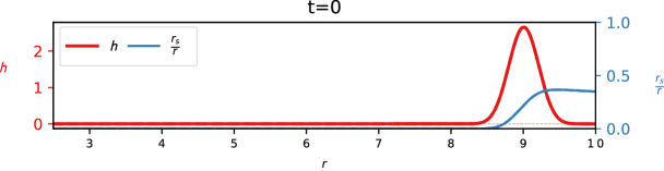
Figure 1: The initial normal ordered Hamiltonian density $h=\frac{\alpha}{2a}h_{r}$ and the ratio of the local Schwarzschild radius $r_{s}=r-d$ to the local radius.

Performing the time evolution of our system in both the classical and the semiclassical cases, we observe the onset of horizon formation (see fig. 2), which seems to happen at larger radial coordinates in the semiclassical case.

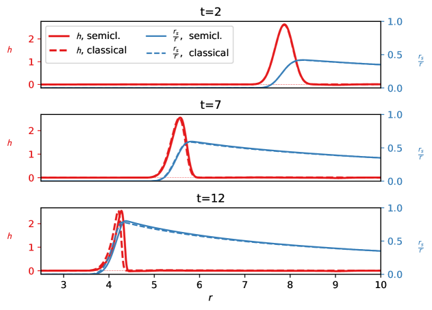
Figure 2: Time evolution of the state from fig. 1.

In order to highlight the difference between the classical and semiclassical cases in the $l=0$ approximation, we can plot the vacuum terms alone. We can in fact do this for the classical case, where we can measure the vacuum term even though it does not contribute to the time evolution. In fig. 3 we have plotted the corresponding terms, providing evidence that within our approximation the vacuum in both the semiclassical and the classical time evolution tend to enhance the peak energy density.

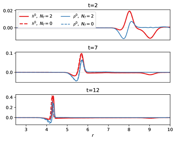
Figure 3: The vacuum part of the Hamiltonian density for the Hamiltonian density $h^{0}$ and the radial momentum density $p^{0}=\frac{\alpha}{2a}p^{0}_{r}$ for three different times in the evolution. Note the different scales of the $y$-axis in the three plots. The static dip around $r=9$ is a remnant of our initial state vacuum definition.

In fig. 4, we zoom in on the vacuum contribution of the semiclassical time evolution at $t=12$. In addition to the vacuum term with respect to the initial metric, we have also plotted the vacuum term with respect to the current metric in the time evolution. The latter is obtained by not subtracting $h_{0}(t)$, but instead by computing a new $h_{0}(t_{0})$ according to (6) with the evolution coefficients reinitialised at $t_{0}=t$ as in (3). One can see, that with respect to the initial state metric, the vacuum term enhances the peak region while depressing both outer and inner flanks, whereas with respect to the current state metric, the vacuum contribution is negative inside the peak region and positive just outside.

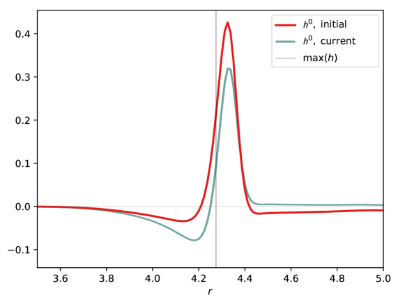
Figure 4: Comparison of the vacuum energy contribution at $t=12$ as seen with respect to the either the initial or current metric vacuum energy subtraction. The vertical line corresponds to the maximum of the total Hamiltonian density at this time.

5 Conclusions and outlook

We are investigating the semiclassical gravitational collapse of a massless scalar field. While the formalism seems to work in principle and yields interesting first results in the $l=0$ approximation, there still is a lot of conceptual work to be done. Most importantly, we want to go beyond the $l=0$ approximation, which requires additional regularization. We are currently in the process of investigating different approaches, including static mode subtraction, point splitting and the introduction of Pauli-Villars fields as suggested in [6, 5]. There are also a number of technical challenges, such as instabilities in the eigenmode decomposition near the origin or the proper treatment of high frequency modes close to a forming horizon, which have to be overcome before more physical conclusions about the behaviour of the system can be drawn.

References

• [1] S.W. Hawking. Particle Creation by Black Holes. Commun. Math. Phys., 43:199–220, 1975. [Erratum: Commun.Math.Phys. 46, 206 (1976)].
• [2] Daniel Harlow. Jerusalem Lectures on Black Holes and Quantum Information. Rev. Mod. Phys., 88:15002, 2016.
• [3] Samir D. Mathur. The Information paradox: A Pedagogical introduction. Class. Quant. Grav., 26:224001, 2009.
• [4] Jana N. Guenther, Christian Hoelbling, and Lukas Varnhorst. Semiclassical gravitational collapse of a radially symmetric massless scalar quantum field. 10 2020.
• [5] Benjamin Berczi, Paul M. Saffin, and Shuang-Yong Zhou. Gravitational collapse of quantum fields and Choptuik scaling. 11 2021.
• [6] Benjamin Berczi, Paul M. Saffin, and Shuang-Yong Zhou. Gravitational collapse with quantum fields. Phys. Rev. D, 104(4):0, 2021.
• [7] Matthew W. Choptuik. Universality and scaling in gravitational collapse of a massless scalar field. Phys. Rev. Lett., 70:9–12, 1993.
• [8] D. Christodoulou. The Problem of a Selfgravitating Scalar Field. Commun. Math. Phys., 105:337–361, 1986.
• [9] D. Christodoulou. A Mathematical Theory of Gravitational Collapse. Commun. Math. Phys., 109:613–647, 1987.
• [10] Dalia S. Goldwirth and Tsvi Piran. Gravitational Collapse of Massless Scalar Field and Cosmic Censorship. Phys. Rev. D, 36:3575, 1987.
• [11] A. Nuttall. Some windows with very good sidelobe behavior. IEEE Transactions on Acoustics, Speech, and Signal Processing, 29(1):84–91, 1981.