Scaling approach to nuclear structure in high-energy heavy-ion collisions

Abstract

In high-energy heavy-ion collisions, the initial condition of the produced quark-gluon plasma (QGP) and its evolution are sensitive to collective nuclear structure parameters describing the shape and radial profiles of the nuclei. We find a general scaling relation between these parameters and many experimental observables such as elliptic flow, triangular flow, and particle multiplicity distribution. In particular, the ratios of observables between two isobar systems depend only on the differences of these parameters, but not on the details of the final state interactions, hence offering a new way to constrain the QGP initial condition. Using this scaling relation, we show how the structure parameters of ${}^{96}_{44}$Ru and ${}^{96}_{40}$Zr conspire to produce the rich centrality dependences of these ratios, as measured by the STAR Collaboration. Our scaling approach demonstrates that isobar collisions are a precision tool to probe the initial condition of heavy-ion collisions, as well as the collective nuclear structures, including the neutron skin, of the atomic nuclei across energy scales.

One main challenge in nuclear physics is to map out the shape and radial structure of the atomic nuclei and understand how they emerge from the interactions among the constituent nucleons Nakatsukasa et al. (2016); Nazarewicz (2016). Varying the number of nucleons along isotopic/isotonic chain often induces rich and non-monotonic changes in the nuclear structure properties. In certain regions of nuclear chart, for example, even adding or subtracting a few nucleons can induce significant deformations and/or changes in the nuclear radius or neutron skin Möller et al. (2016); Cao et al. (2020); Angeli and Marinova (2013); Centelles et al. (2009). Experimental information on nuclear structure is primarily obtained by spectroscopic or scattering measurements at low energies. But studies show that nuclear structure can be probed in high-energy nuclear collisions at the relativistic heavy ion collider (RHIC) and the large hadron collider (LHC) Tanihata et al. (1985); Rosenhauer et al. (1986); Li (2000); Heinz and Kuhlman (2005); Filip et al. (2009); Shou et al. (2015); Goldschmidt et al. (2015); Giacalone et al. (2018); Giacalone (2020a, b); Giacalone et al. (2021a, b); Jia et al. (2022a); Jia (2022a); Bally et al. (2022), and experimental evidences have been observed Adamczyk et al. (2015); Acharya et al. (2018); Sirunyan et al. (2019); Aad et al. (2020); Jia .

The connection between nuclear structure and high-energy heavy-ion collisions is illustrated in Fig. 1. These collisions deposit a large amount of energy in the overlap region in the middle panel, forming a hot and dense quark-gluon plasma (QGP) Busza et al. (2018). Driven by large pressure gradients, the QGP undergoes a hydrodynamical expansion, converting the initial spatial anisotropies into momentum anisotropies of particles in the final state in the right panel. Observables describing the collective features of the particles in the final state, such as elliptic flow $v_{2}$, triangular flow $v_{3}$ and charged particle multiplicity $N_{\mathrm{ch}}$ are closely related to geometric features of the initial condition, ellipticity $\varepsilon_{2}$, triangularity $\varepsilon_{3}$ and number of participating nucleons $N_{\mathrm{part}}$, respectively. In fact, at energies reached at RHIC and the LHC, $\mbox{$\sqrt{s_{\mathrm{NN}}}$}\geq 100$ GeV, these quantities are linearly-related $v_{n}\propto\varepsilon_{n}$ and $N_{\mathrm{ch}}\propto N_{\mathrm{part}}$ Teaney and Yan (2012); Niemi et al. (2016). On the other hand, the shape and size of the initial condition are affected by the nucleon distribution in the colliding nuclei in the left panel, often described by a deformed Woods-Saxon (WS) density,

$$\rho(r,\theta,\phi) \propto\frac{1}{1+e^{[r-R_{0}\left(1+\beta_{2}Y_{2}^{0}(\theta,\phi)+\beta_{3}Y_{3}^{0}(\theta,\phi)\right)]/a}},$$ (1)

containing four structure parameters: quadrupole deformation $\beta_{2}$ and octupole deformation $\beta_{3}$, half-density radius $R_{0}$, and surface diffuseness $a$ Horiuchi (2021). The deformation $\beta_{2}$ ($\beta_{3}$) enhances the $\varepsilon_{2}$ ($\varepsilon_{3}$) in the initial condition Heinz and Kuhlman (2005); Carzon et al. (2020); Jia (2022a). A change in $a$ influences $\varepsilon_{n}$ and charge particle multiplicity distribution $p(N_{\mathrm{part}})$ Shou et al. (2015); Li et al. (2018). Both $a$ and $R_{0}$ were shown to have significant impact on the initial overlap area Zhang et al. (2022); Xu et al. (2021a). In more recent studies, these structure parameters are found to have much larger impact on multi-point correlators in both the initial and final state Zhao et al. (2022); Jia et al. (2022b, c). Understanding the role of nuclear structure can improve modeling of the initial condition, which currently limits the extraction of the transport properties of the QGP Bernhard et al. (2016); Everett et al. (2021a); Nijs et al. (2021).

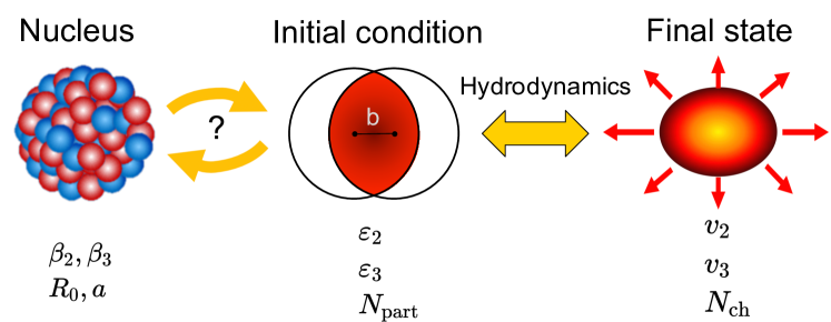
Figure 1: Connection between collective nuclear structure (left), the initial condition (middle) and final state (right) of high-energy heavy-ion collisions, together with parameters describing the geometrical aspects for each phase (see text). Due to the extremely short nuclear crossing time $2R_{0}/\gamma\lesssim 0.1$ fm/$c$, the initial condition is well separated from the hydrodynamical evolution in the final state. The geometry of the initial condition depends on the impact parameter $b$ and structure parameters.

Due to the dominant role of the impact parameter, earlier studies focused on the most central collisions where the impact of nuclear structure can be easily identified. It is realized recently that the nuclear structure impact can be cleanly isolated over the full centrality range by comparing two isobaric collision systems Giacalone et al. (2021a, b). Since isobar nuclei have the same mass number but different structures, deviation from unity of the ratio of any observable must originate from differences in the structure of the colliding nuclei, which impact the initial state of QGP and its final state evolution. Collisions of one such pair of isobar systems, ⁹⁶Ru+⁹⁶Ru and ⁹⁶Zr+⁹⁶Zr, have been performed at RHIC. Ratios of many observables are found to show significant and centrality-dependent departures from unity Abdallah et al. (2022). The goal of this Letter is to explore the scaling behavior of these ratios with respect to the WS parameters in Eq. (1).

We illustrate this point using three heavy-ion observables, the $v_{2}(N_{\mathrm{ch}})$, $v_{3}(N_{\mathrm{ch}})$ and $p(N_{\mathrm{ch}})$, although the same idea applies to many other single-particle or two-particle observables. For small deformations and small variations of $R_{0}$ and $a$ from their default reference values, the observable $\mathcal{O}$ has the following leading-order form,

$$\mathcal{O}\approx b_{0}+b_{1}\beta_{2}^{2}+b_{2}\beta_{3}^{2}+b_{3}(R_{0}-R_{0,\mathrm{ref}})+b_{4}(a-a_{\mathrm{ref}})\;,$$ (2)

where $b_{0}$ is the value for spherical nuclei at some reference radius and diffuseness, and $b_{1}$–$b_{4}$ are centrality-dependent response coefficients that encode the final-state dynamics. . Most dependence on mass number is carried by $b_{0}$, while $b_{1}$–$b_{4}$ are expected to be weak functions of mass number. The ratio of $\mathcal{O}$ between ⁹⁶Ru+⁹⁶Ru and ⁹⁶Zr+⁹⁶Zr then has a simple scaling relation

$$R_{\mathcal{O}}\equiv\frac{\mathcal{O}_{\mathrm{\mathrm{Ru}}}}{\mathcal{O}_{\mathrm{\mathrm{Zr}}}}\approx 1+c_{1}\Delta\beta_{2}^{2}+c_{2}\Delta\beta_{3}^{2}+c_{3}\Delta R_{0}+c_{4}\Delta a\;,$$ (3)

where $\Delta\beta_{n}^{2}=\beta_{n,\mathrm{\mathrm{Ru}}}^{2}-\beta_{n,\mathrm{\mathrm{Zr}}}^{2}$, $\Delta R_{0}=R_{0,\mathrm{\mathrm{Ru}}}-R_{0,\mathrm{\mathrm{Zr}}}$, $\Delta a=a_{\mathrm{\mathrm{Ru}}}-a_{\mathrm{\mathrm{Zr}}}$ and $c_{n}=b_{n}/b_{0}$. Two important insights can be drawn if Eq. (3) holds: 1) these ratios can only probe the difference in the WS parameters between the isobar nuclei, 2) the contributions are independent of each other among the WS parameters.

To verify this scaling relation, we simulate the dynamics of the QGP using the multi-phase transport model (AMPT) Lin et al. (2005). The AMPT model describes collective flow data at RHIC and the LHC Xu and Ko (2011); Abdallah et al. (2021) and was used to study the $\beta_{n}$ dependence of $v_{n}$ Giacalone et al. (2021b); Zhang and Jia (2022). We use AMPT v2.26t5 in string-melting mode at $\mbox{$\sqrt{s_{\mathrm{NN}}}$}=200$ GeV with a partonic cross section of 3.0 $m$b Ma and Bzdak (2014); Bzdak and Ma (2014). We simulate generic isobar ⁹⁶X+⁹⁶X collisions covering a wide range of $\beta_{2}$, $\beta_{3}$, $R_{0}$ and $a$, including the default values assumed for ⁹⁶Ru and ⁹⁶Zr listed in Table 1. Following Ref. Xu et al. (2021b), the default values are taken from Ref. Fricke et al. (1995) for $R_{0}$ or deduced from neutron skin data Trzcinska et al. (2001) for $a$. The default values of $\beta_{2}$ and $\beta_{3}$ are taken from Ref. Zhang and Jia (2022). The $v_{n}$ are calculated using two-particle correlation method with hadrons of $0.2<p_{\mathrm{T}}<2$ GeV and $|\eta|<2$ Aad et al. (2012). The ratios are calculated as a function of $N_{\mathrm{ch}}$ instead of centrality, because the ratios calculated at the same $N_{\mathrm{ch}}$ have a good cancellation of non-flow contributions Jia et al. (2022d) and the final state effects Zhang et al. (2022).

Species	$\beta_{2}$	$\beta_{3}$	$a$	$R_{0}$
96Ru	0.162	0	0.46 fm	5.09 fm
96Zr	0.06	0.20	0.52 fm	5.02 fm
difference	$\Delta\beta_{2}^{2}$	$\Delta\beta_{3}^{2}$	$\Delta a$	$\Delta R_{0}$
	0.0226	-0.04	-0.06 fm	0.07 fm

Table 1: Collective nuclear structure parameters for ⁹⁶Ru and ⁹⁶Zr and the differences.

To explore the parametric dependence of the hydrodynamic response, the parameters are varied one at a time. The $\beta_{2}$ is changed from 0 to 0.1, 0.15 and 0.2; the $\beta_{3}$ is changed from 0 to 0.1, 0.2 and 0.25; the $a$ is varied from 0.52 fm to 0.46 fm, 0.40 fm and 0.34 fm; the $R_{0}$ is varied from 5.09 fm to 5.02 fm, 4.8 fm and 4.5 fm. An independent sample is generated for each case and the $v_{2}$, $v_{3}$ and $p(N_{\mathrm{ch}})$ are calculated. The change in the ratios from unity, $R_{\mathcal{O}}-1$, are scaled according to the actual differences between Ru and Zr listed in Table 1. The results for all twelve cases (four parameters times three observables) as a function of $N_{\mathrm{ch}}$ are summarized in Fig. 2.

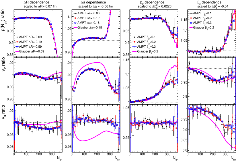
Figure 2: The four terms of Eq. (3) associated with $R_{0}$ (left column), $a$ ($2^{\mathrm{nd}}$ column), $\beta_{2}$ ($3^{\mathrm{rd}}$ column) and $\beta_{3}$ (right column) from the AMPT model for ratios of $p(N_{\mathrm{ch}})$ (first row), $v_{2}$ (middle row) and $v_{3}$ (bottom row). Distribution in each panel is determined for several values of parameters and scaled to the same default value. They are compared with those obtained for quark Glauber model (solid lines).

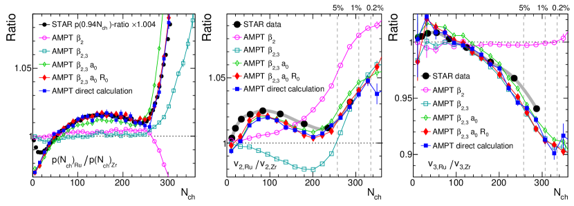
Figure 3: The ratios of $p(N_{\mathrm{ch}})$ (left panel), $v_{2}$ (middle panel), and $v_{3}$ (right panel) from AMPT using the default nuclear structure parameters in Tab. 1 (labeled “direct calculation”) or calculated step-by-step from the response coefficients from Fig. 2. The $N_{\mathrm{ch}}$ and $R_{p(N_{\mathrm{ch}})}$ values from data have been scaled by 0.94 and 1.004, respectively to match the AMPT. Note also that the STAR $v_{n}$ ratios at the same centrality Abdallah et al. (2022) has been corrected to reflect the ratio at the same $N_{\mathrm{ch}}$ Jia et al. (2022d).

One striking feature is the nearly perfect scaling of $R_{\mathcal{O}}$ over the wide range of parameter values studied. The shapes of these dependences reflect directly the response coefficients $c_{n}(N_{\mathrm{ch}})$ for each observable. The statistical uncertainties of $c_{n}$ decrease for larger variations of the WS parameters, implying that the $c_{n}$ can be determined more precisely by using a larger change of each parameter. This has the benefit of significantly reducing the number of events required in the hydrodynamic model simulation to achieve the desired precision, ideally suitable for the multi-system Bayesian global analyses of heavy-ion collisions Nijs et al. (2021); Everett et al. (2021b).

All the WS parameters do not have the same influences on final state observables. In peripheral and mid-central collisions, the ratio $p(N_{\mathrm{ch}})_{\mathrm{Ru}}/p(N_{\mathrm{ch}})_{\mathrm{Zr}}$ is influenced mostly by the $\Delta a$ and $\Delta R_{0}$. In particular, the characteristic broad peak and non-monotonic behavior of the ratio is a clear signature of the influence of $\Delta a$ Xu et al. (2021b). In the most central collisions, the ratio is sensitive to all four parameters. The influence of WS parameters on $v_{2,\mathrm{Ru}}/v_{2,\mathrm{Zr}}$ is more rich: 1) in the most central collisions, the ratio is mainly dominated by $\Delta\beta_{2}^{2}$ and to a lesser extent by $\Delta\beta_{3}^{2}$; 2) in the near-central collisions, the ratio is influenced by a positive contribution from $\Delta\beta_{2}^{2}$ and a larger negative contribution from $\Delta\beta_{3}^{2}$; 3) in the mid-central and peripheral collisions, the impact of $\Delta a$ is more important; 4) the influence of $\Delta R_{0}$ is negligible except in central collisions. Lastly, the ratio $v_{3,\mathrm{Ru}}/v_{3,\mathrm{Zr}}$ is mainly influenced by $\Delta\beta_{3}^{2}$, although $\Delta a$ and $\Delta R_{0}$ have opposite up to 1% contributions over a broad $N_{\mathrm{ch}}$ range.

The scaling relation in Fig. (2) allows us to construct directly the ratios of experimental observables for any values of $\Delta\beta_{2}^{2}$, $\Delta\beta_{3}^{2}$, $\Delta a$ and $\Delta R_{0}$, without the need to carry out additional simulations. One could also perform a simultaneous fit of several experimental ratios to obtain the optimal values of these parameters within a given model framework and expose its limitations. Figure 3 shows a step-by-step construction of the prediction in comparison with the STAR data. Each panel also shows the ratio obtained directly from a separate AMPT simulation of ⁹⁶Ru+⁹⁶Ru and ⁹⁶Zr+⁹⁶Zr collisions using the default parameters in the Table 1. Excellent agreement is obtained between the construction approach and the direct calculation, attesting to the robustness of our proposed method. Also for the first time, we achieved simultaneous description of all three ratios using one set of WS parameters in most centrality ranges.

One natural question is how these isobar ratios are influenced by various final state effects. A recent study from us has demonstrated explicitly that isobar ratios are insensitive to the shear viscosity, hadronization and hadronic transport Zhang et al. (2022). Therefore, any model dependence in the isobar ratios must reflect a model dependence in the initial condition, i.e. how the energy is deposited in the overlap region (see Fig. 1). One example is the response functions calculated from a quark Glauber model shown in Fig. 2 (details in Supplemental materials), which has clear differences in several cases from the AMPT model. There are potentially many initial conditions, reflected by the well-known T_RENTo formula for the energy density $e(x,y)\propto\left(T_{\mathrm{A}}^{p}+T_{\mathrm{B}}^{p}\right)^{q/p}$ calculated from the thickness function $T_{\mathrm{A}}$ and $T_{\mathrm{B}}$ of colliding ions, where each $q$ and $p$ value specify a different initial condition Moreland et al. (2015); Nijs and van der Schee (2022). The coefficients $c_{n}$ provide a new way to constrain the initial condition by exploiting structure differences between isobars. One has to first calibrate the values of $c_{n}$ using species whose WS parameters are relatively well known. The calibrated $c_{n}$ can then be used to 1) narrow the $q$ and $p$ values, which can be subsequently fixed in the Bayesian inference to improve the extraction of the QGP properties, and 2) constrain the nuclear structure parameters for species of interest by directly fitting Eq. (3) to the measured isobar ratios.

A caveat is in order regarding to the connection between nuclear structure and initial condition. The parameters describing the shape of the nuclei in high energy may not take the same values as those at low-energy. In fact, nuclear structure at small partonic longitudinal momentum fraction (small-$x$), is expected to be modified due to gluon shadowing or saturation effects, described by nPDF or nuclear partonic distribution function. The nPDF appears as additional spatial modulation of the nucleon distribution in the transverse plane, and will modify the values of the parameters in Eq. (1) in a $x$-dependent way. The nPDF effects, as input to the heavy-ion initial condition, is a key topic in $e$+A collisions at future electron-ion collider (EIC) and $p$+A collisions. The isobar collisions provide a new means to access modification of nuclear structure in dense gluon environment in a data-driven approach, for example by comparing isobar ratios between RHIC and the LHC energies or as a function of rapidity.

The scaling approach discussed above can be extended to compare collisions of systems with similar but slightly different mass number $A$, ideally along an isotopic chain. As the $N_{\mathrm{ch}}$ distribution scales approximately with $A$, the ratios of experimental observable can be obtained as a function of $N_{\mathrm{ch}}/(2A)$ or centrality. In this case, one has $b_{0}\rightarrow b_{0}(1+\frac{d\ln b_{0}}{d\ln A}\frac{\Delta A}{A})$, which leads to one additional term, $\frac{d\ln b_{0}}{d\ln A}\frac{\Delta A}{A}$, in Eq. (3). The $A$ dependence of $c_{n}$ is weak and also its contribution to Eq. (3) has a higher-order form, e.g. $\frac{\Delta A}{A}\Delta a$, etc., therefore is ignored. Studies along this line have been done for elliptic flow Giacalone et al. (2021b); Jia (2022a), which show that the $b_{0}$ for $\epsilon_{2}$ has the form $b_{0}\propto 1/A$ in the ultra-central collisions, and that $R_{\epsilon_{2}}$ receives an additional correction $-\Delta A/A$. This contribution should be quantified for each observable and compared to data from two systems of similar sizes, such as ¹⁹⁷Au+¹⁹⁷Au and ²³⁸U+²³⁸U. In conjunction with the scaling relations for the nuclear structure parameters discussed above, they can be a powerful tool in understanding the system size dependence of heavy-ion observables.

The scaling approach also provides a clean way to probe the difference between the root mean square radius of neutrons and protons in heavy nuclei, $\Delta r_{np}=R_{n}-R_{p}$, known as the neutron skin. The $\Delta r_{np}$ is related to the symmetry energy contribution to the equation of state (EOS): a quantity of fundamental importance in nuclear- and astro-physics Lattimer and Prakash (2007); Li et al. (2008). From discussion above, the isobar ratios are expected to probe only the difference in the neutron skin. To see this, we first express the mean square radius of nucleon distribution in Eq. (1) by $R^{2}\approx(\frac{3}{5}R_{0}^{2}+\frac{7}{5}\pi^{2}a^{2})/(1+\frac{5}{4\pi}\sum_{n}\beta_{n}^{2})$ Bohr and Mottelson (1998). The neutron skin is then expressed in terms of the differences between nucleon distribution and proton distribution:

$$\Delta r_{np}\!=\!\frac{R^{2}-R_{p}^{2}}{R(\delta\!+\!1)}\! \approx\!\frac{3(R_{0}^{2}\!-\!R_{0,p}^{2})\!+\!7\pi^{2}(a^{2}\!-\!a_{p}^{2})}{\sqrt{15}R_{0}\sqrt{1\!+\!\frac{7\pi^{2}}{3}\!\frac{a^{2}}{R_{0}^{2}}}(1\!+\!\delta\!+\!\frac{5}{8\pi}\!\sum_{n}\beta_{n}^{2})},$$ (4)

where $\delta=(N-Z)/A$, and $R_{0,p}$ and $a_{p}$ are the well-measured WS parameters for the proton distribution Fricke et al. (1995). Simple algebraic manipulation shows that $\Delta R_{0}$ and $\Delta a$ are related to the skin difference sup ,

$$\Delta(\Delta r_{np})\approx- \overline{\Delta r}_{np}(\frac{\Delta\delta}{1\!+\!\bar{\delta}}+\frac{\Delta R_{0}}{\bar{R}_{0}})+$$

$$\frac{\Delta Y-\frac{7\pi^{2}}{6}\frac{\bar{a}^{2}}{\bar{R}_{0}^{2}}\left(\Delta Y+2\bar{Y}(\frac{\Delta a}{\bar{a}}-\frac{\Delta R_{0}}{\bar{R}_{0}})\right)}{\sqrt{15}\bar{R}_{0}(1+\bar{\delta}+\frac{5}{8\pi}\sum_{n}\overline{\beta_{n}^{2}})}\;,$$ (5)

where $\bar{x}$ represents the average of $x$ between the two systems, and $Y\equiv 3(R_{0}^{2}\!-\!R_{0,p}^{2})\!+\!7\pi^{2}(a^{2}\!-\!a_{p}^{2})$. The term associated with $\overline{\Delta r}_{np}$ can be dropped if we ignore change of $\delta$ and $R_{0}$, which is typically a few percents of $\overline{\Delta r}_{np}$ for isobar systems. The numerator of Eq. (5) is dominated by $\Delta Y=6(\bar{R}_{0}\Delta R_{0}\!-\!\bar{R}_{0p}\Delta R_{0p})\!+\!14\pi^{2}(\bar{a}\Delta a\!-\!\bar{a}_{p}\Delta a_{p})$, the remaining term is on the order of $\frac{7\pi^{2}}{6}\frac{\bar{a}^{2}}{\bar{R}_{0}^{2}}\sim 11(0.5/5)^{2}=11\%$ of $\Delta Y$. We checked that the Eq. (5) is accurate within 2% using parameters for ⁹⁶Ru and ⁹⁶Zr listed in Ref. Xu et al. (2021b).

Knowledge of nucleon distribution gives direct information on the neutron skin, once it is combined with the well-known proton distribution. Eq. (5) shows that isobar data can only constrain the neutron skin difference, which can be constructed from $\Delta R_{0}$ and $\Delta a$, together with well-measured $\Delta R_{0,p}$ and $\Delta a_{p}$ for protons. The neutron skin difference is sensitive to both $\Delta R_{0}$ (skin-type contribution) and $\Delta a$ (halo-type contribution) Trzcinska et al. (2001); Centelles et al. (2010). Previous studies of neutron skin are done by inputting density functional theory (DFT) calculation of nuclear structure directly to the hydrodynamic modeling of heavy-ion collisions Li et al. (2020); Xu et al. (2021a, b). The neutron skin values are constrained by comparing directly with experimental observables. What we are proposing here is to decouple DFT from modeling of heavy-ion collisions. One first extracts the $\Delta R_{0}$ and $\Delta a$ values consistent with many isobar ratios using the scaling approach, which are then compared with those calculated directly from nucleon distributions from the DFT theory. Eq. (5) provides an easy way to estimate the skin difference, and contributions from skin-type or halo-type.

In summary, we presented a new approach to constrain the collective nuclear structure parameters in high-energy heavy-ion isobar collisions. We found that the changes in the final state observables $v_{2}(N_{\mathrm{ch}})$, $v_{3}(N_{\mathrm{ch}})$ and $p(N_{\mathrm{ch}})$ follow a simple dependence on the variation of these parameters. The coefficients of these variations can be determined precisely in a given model framework, and subsequently used to make predictions of observables at other parameter values. This scaling behavior is particularly useful in analyzing the ratios between isobar systems, such as ⁹⁶Ru+⁹⁶Ru and ⁹⁶Zr+⁹⁶Zr collisions measured by the STAR experiment Abdallah et al. (2022). We show that the STAR data can constrain directly the nuclear structure differences between ⁹⁶Ru and ⁹⁶Zr (compatible with the structure values in Tab. 1). Since these isobar ratios are also found to be insensitive to the details of interaction in the final state, the isobar collisions serve as a precise tool for accessing both the bulk nuclear structure parameters and the initial condition of heavy-ion collisions. The extracted information on nucleon distribution, together with well-measured charge distribution, can probe the difference in the neutron skin between large isobar systems. However, future measurements of isobar ratios as a function of collision energy and rapidity, are necessary to quantify the modification of nuclear structure at high-energy across energy scales, and establish more firmly the connection between nuclear structure and the initial condition. Our study demonstrates the unique opportunities offered by relativistic collisions of isobars as a tool to perform inter-disciplinary nuclear physics studies, which we hope will be pursued in future by collisions of several isobar pairs in collider facilities.

Acknowledgements: We thank Giuliano Giacalone, Che-Ming Ko, Bao-An Li and Jun Xu for careful reading and valuable comments on the manuscript. This work is supported by DOE DE-FG02-87ER40331.

Supplemental materials

To show how Eq. (5) is derived, we note that the ms radii for nucleon, neutron and proton distributions are related by

$$R^{2}=\frac{1+\delta}{2}R_{n}^{2}+\frac{1-\delta}{2}R_{p}^{2}\;.$$ (6)

This leads to $\Delta r_{np}\frac{R_{n}+R_{p}}{2}=\frac{R^{2}-R_{p}^{2}}{1+\delta}$, and together with the approximation $R_{n}+R_{p}\approx 2R-\delta\Delta r_{np}$, we get

$$\Delta r_{np}(1-\frac{\Delta r_{np}\delta}{2R})=\frac{R^{2}-R_{p}^{2}}{R(1+\delta)}\;.$$ (7)

Ignoring the $\Delta r_{np}\delta/(2R)$ term, which is typically much less than 1%, we obtain Eq. (4). To derive Eq. (5), we first rewrite Eq. (4) as,

$$\Delta r_{np} \sqrt{15}R_{0}(1+\delta\!+\!\frac{5}{8\pi}\!\sum_{n}\beta_{n}^{2})\approx$$

$$(3(R_{0}^{2}\!-\!R_{0,p}^{2})\!+\!7\pi^{2}(a^{2}\!-\!a_{p}^{2}))(1-\frac{7\pi^{2}}{6}\frac{a^{2}}{R_{0}^{2}})\;,$$ (8)

where we have ignored the high-order term $\mathcal{O}(\frac{a^{4}}{R_{0}^{4}})$ on the right hand side (rhs), which is much less than 1% for medium and large nuclei. We now consider the difference of two such expressions for two isobars, labelled by “1” and “2”, respectively. We shall use the relations $x_{1}y_{1}-x_{2}y_{2}=\Delta x\bar{y}+\Delta y\bar{x}$ and $x_{1}y_{1}z_{1}-x_{2}y_{2}z_{2}=\Delta x\bar{y}\bar{z}+\Delta y\bar{x}\bar{z}+\Delta z\bar{x}\bar{y}+\frac{1}{4}\Delta x\Delta y\Delta z$, where $\Delta x=x_{1}-x_{2}$ and $\bar{x}=(x_{1}+x_{2})/2$ etc. Then, the left hand side (lhs) of Eq. (8) can be written as,

$$\Delta(\mathrm{lhs})/\sqrt{15} =\Delta\left[\Delta r_{np}R_{0}(1+\delta+\frac{5}{8\pi}\sum_{n}\beta_{n}^{2})\right]$$

$$\approx\Delta(\Delta r_{np})\bar{R}_{0}(1+\bar{\delta}+\frac{5}{8\pi}\sum_{n}\overline{\beta_{n}^{2}})$$

$$+\overline{\Delta r}_{np}\bar{R}_{0}(\frac{\Delta R_{0}}{\bar{R}_{0}}(1+\bar{\delta})+\Delta\delta+\frac{5}{8\pi}\!\sum_{n}\!\Delta\beta_{n}^{2})\;.$$ (9)

For the rhs of Eq. (8), it can be written as,

$$\Delta(\mathrm{rhs}) =\Delta\left[(3(R_{0}^{2}\!-\!R_{0,p}^{2})\!+\!7\pi^{2}(a^{2}\!-\!a_{p}^{2}))(1-\frac{7\pi^{2}}{6}\frac{a^{2}}{R_{0}^{2}})\right]$$

$$=\Delta Y-\frac{7\pi^{2}}{3}\frac{\bar{a}^{2}}{\bar{R}_{0}^{2}}\left(\frac{\Delta Y}{2}+\bar{Y}(\frac{\Delta a}{\bar{a}}-\frac{\Delta R_{0}}{\bar{R}_{0}})\right)\;,$$ (10)

with $Y\equiv 3(R_{0}^{2}\!-\!R_{0,p}^{2})\!+\!7\pi^{2}(a^{2}\!-\!a_{p}^{2})$. Eq. (5) is then obtained by combining Eq. (9) and Eq. (10).

To further understand the behaviors of various response coefficients, we also performed a calculation based on the quark Glauber model discussed in Refs. Jia (2022b, a), where each nucleon is replaced by three constituent quarks. The distribution of quark-participants $p(N_{\mathrm{quark}})$ generated for the parameter set of ⁹⁶Ru in Table 1 is then convoluted with a negative binomial distribution that describes the production of charged particle for each participant, $p_{\mathrm{nbd}}(n)=\frac{(n+m-1)!}{(m-1)!n!}\frac{\bar{n}^{n}m^{m}}{(\bar{n}+m)^{n+m}}$. The convoluted distribution is tuned to match the published $p(N_{\mathrm{ch}})_{\mathrm{Ru}}$, giving the best fit values of $\bar{n}=0.6535$ and $m=0.7515$. These values are then used to generate the $p(N_{\mathrm{ch}})$ for all other WS parameters. We then calculate the $\varepsilon_{n}$ as a function of $N_{\mathrm{ch}}$ and obtain the ratios $\varepsilon_{n,\mathrm{Ru}}/\varepsilon_{n,\mathrm{Zr}}$ as an estimator for $v_{n,\mathrm{Ru}}/v_{n,\mathrm{Zr}}$. Figure 4 shows the ratios of $p(N_{\mathrm{ch}})$, $\varepsilon_{2}$ and $\varepsilon_{3}$ obtained in the quark Glauber model for several values of $R_{0}$, $a$, $\beta_{2}$ and $\beta_{3}$ relative to the default. The corresponding ratios after being scaled to the default variation as listed in Table 1 are shown in Fig. 5. Some small deviation from this scaling is observed only when the variations are very large.

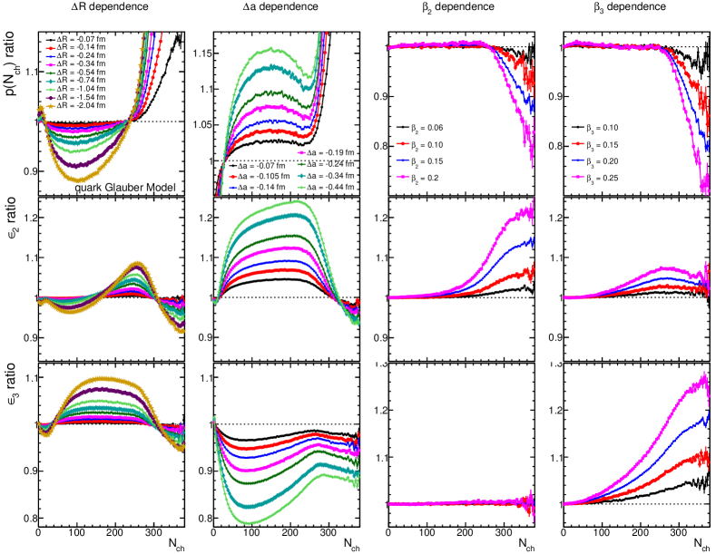
Figure 4: The four response coefficients of Eq. (3) for variation of nuclear structure parameters $R_{0}$ (left column), $a$ (2nd column), $\beta_{2}$ (third column) and $\beta_{3}$ (right column) in the quark Glauber model for ratios of $p(N_{\mathrm{ch}})$ (first row), $\varepsilon_{2}$ (middle row) and $\varepsilon_{3}$ (bottom row). Each coefficient in each panel is determined for several values of the parameters and scaled to the same default value.

Figure 5: Information in Fig. 4 scaled to the default variation in the nuclear structure parameters as indicated in the top of each column. Only selected cases are shown for variations in parameters $R_{0}$ and $a$ in order to make the plots less busy.

References

- Nakatsukasa et al. (2016) Takashi Nakatsukasa, Kenichi Matsuyanagi, Masayuki Matsuo, and Kazuhiro Yabana, “Time-dependent density-functional description of nuclear dynamics,” Rev. Mod. Phys. 88, 045004 (2016), arXiv:1606.04717 [nucl-th] .
- Nazarewicz (2016) Witold Nazarewicz, “Challenges in Nuclear Structure Theory,” J. Phys. G 43, 044002 (2016), arXiv:1603.02490 [nucl-th] .
- Möller et al. (2016) P. Möller, A. J. Sierk, T. Ichikawa, and H. Sagawa, “Nuclear ground-state masses and deformations: FRDM(2012),” Atom. Data Nucl. Data Tabl. 109-110, 1–204 (2016), arXiv:1508.06294 [nucl-th] .
- Cao et al. (2020) Yuchen Cao, Sylvester E. Agbemava, Anatoli V. Afanasjev, Witold Nazarewicz, and Erik Olsen, “Landscape of pear-shaped even-even nuclei,” Phys. Rev. C 102, 024311 (2020), arXiv:2004.01319 [nucl-th] .
- Angeli and Marinova (2013) I. Angeli and K. P. Marinova, “Table of experimental nuclear ground state charge radii: An update,” Atom. Data Nucl. Data Tabl. 99, 69–95 (2013).
- Centelles et al. (2009) M. Centelles, X. Roca-Maza, X. Vinas, and M. Warda, “Nuclear symmetry energy probed by neutron skin thickness of nuclei,” Phys. Rev. Lett. 102, 122502 (2009), arXiv:0806.2886 [nucl-th] .
- Tanihata et al. (1985) I. Tanihata, H. Hamagaki, O. Hashimoto, Y. Shida, N. Yoshikawa, K. Sugimoto, O. Yamakawa, T. Kobayashi, and N. Takahashi, “Measurements of Interaction Cross-Sections and Nuclear Radii in the Light p Shell Region,” Phys. Rev. Lett. 55, 2676–2679 (1985).
- Rosenhauer et al. (1986) A. Rosenhauer, H. Stocker, J. A. Maruhn, and W. Greiner, “Influence of shape fluctuations in relativistic heavy ion collisions,” Phys. Rev. C 34, 185–190 (1986).
- Li (2000) Bao-An Li, “Uranium on uranium collisions at relativistic energies,” Phys. Rev. C 61, 021903 (2000), arXiv:nucl-th/9910030 .
- Heinz and Kuhlman (2005) Ulrich W. Heinz and Anthony Kuhlman, “Anisotropic flow and jet quenching in ultrarelativistic U + U collisions,” Phys. Rev. Lett. 94, 132301 (2005), arXiv:nucl-th/0411054 .
- Filip et al. (2009) Peter Filip, Richard Lednicky, Hiroshi Masui, and Nu Xu, “Initial eccentricity in deformed 197Au + 197Au and 238U + 238U collisions at GeV at the BNL Relativistic Heavy Ion Collider,” Phys. Rev. C 80, 054903 (2009).
- Shou et al. (2015) Q. Y. Shou, Y. G. Ma, P. Sorensen, A. H. Tang, F. Videbæk, and H. Wang, “Parameterization of Deformed Nuclei for Glauber Modeling in Relativistic Heavy Ion Collisions,” Phys. Lett. B 749, 215–220 (2015), arXiv:1409.8375 [nucl-th] .
- Goldschmidt et al. (2015) Andy Goldschmidt, Zhi Qiu, Chun Shen, and Ulrich Heinz, “Collision geometry and flow in uranium + uranium collisions,” Phys. Rev. C 92, 044903 (2015), arXiv:1507.03910 [nucl-th] .
- Giacalone et al. (2018) Giuliano Giacalone, Jacquelyn Noronha-Hostler, Matthew Luzum, and Jean-Yves Ollitrault, “Hydrodynamic predictions for 5.44 TeV Xe+Xe collisions,” Phys. Rev. C 97, 034904 (2018), arXiv:1711.08499 [nucl-th] .
- Giacalone (2020a) Giuliano Giacalone, “Observing the deformation of nuclei with relativistic nuclear collisions,” Phys. Rev. Lett. 124, 202301 (2020a), arXiv:1910.04673 [nucl-th] .
- Giacalone (2020b) Giuliano Giacalone, “Constraining the quadrupole deformation of atomic nuclei with relativistic nuclear collisions,” Phys. Rev. C 102, 024901 (2020b), arXiv:2004.14463 [nucl-th] .
- Giacalone et al. (2021a) Giuliano Giacalone, Jiangyong Jia, and Vittorio Somà, “Accessing the shape of atomic nuclei with relativistic collisions of isobars,” Phys. Rev. C 104, L041903 (2021a), arXiv:2102.08158 [nucl-th] .
- Giacalone et al. (2021b) Giuliano Giacalone, Jiangyong Jia, and Chunjian Zhang, “Impact of Nuclear Deformation on Relativistic Heavy-Ion Collisions: Assessing Consistency in Nuclear Physics across Energy Scales,” Phys. Rev. Lett. 127, 242301 (2021b), arXiv:2105.01638 [nucl-th] .
- Jia et al. (2022a) Jiangyong Jia, Shengli Huang, and Chunjian Zhang, “Probing nuclear quadrupole deformation from correlation of elliptic flow and transverse momentum in heavy ion collisions,” Phys. Rev. C 105, 014906 (2022a), arXiv:2105.05713 [nucl-th] .
- Jia (2022a) Jiangyong Jia, “Shape of atomic nuclei in heavy ion collisions,” Phys. Rev. C 105, 014905 (2022a), arXiv:2106.08768 [nucl-th] .
- Bally et al. (2022) Benjamin Bally, Michael Bender, Giuliano Giacalone, and Vittorio Somà, “Evidence of the triaxial structure of 129Xe at the Large Hadron Collider,” Phys. Rev. Lett. 128, 082301 (2022), arXiv:2108.09578 [nucl-th] .
- Adamczyk et al. (2015) L. Adamczyk et al. (STAR), “Azimuthal anisotropy in UU and AuAu collisions at RHIC,” Phys. Rev. Lett. 115, 222301 (2015), arXiv:1505.07812 [nucl-ex] .
- Acharya et al. (2018) S. Acharya et al. (ALICE), “Anisotropic flow in Xe-Xe collisions at TeV,” Phys. Lett. B 784, 82–95 (2018), arXiv:1805.01832 [nucl-ex] .
- Sirunyan et al. (2019) Albert M Sirunyan et al. (CMS), “Charged-particle angular correlations in XeXe collisions at 5.44 TeV,” Phys. Rev. C 100, 044902 (2019), arXiv:1901.07997 [hep-ex] .
- Aad et al. (2020) Georges Aad et al. (ATLAS), “Measurement of the azimuthal anisotropy of charged-particle production in collisions at TeV with the ATLAS detector,” Phys. Rev. C 101, 024906 (2020), arXiv:1911.04812 [nucl-ex] .
- (26) Jiangyong Jia, “Nuclear deformation effects via Au+Au and U+U collisions from STAR,” Contribution to the VIth International Conference on the Initial Stages of High-Energy Nuclear Collisions, January 2021, https://indico.cern.ch/event/854124/contributions/4135480/.
- Busza et al. (2018) Wit Busza, Krishna Rajagopal, and Wilke van der Schee, “Heavy Ion Collisions: The Big Picture, and the Big Questions,” Ann. Rev. Nucl. Part. Sci. 68, 339–376 (2018), arXiv:1802.04801 [hep-ph] .
- Teaney and Yan (2012) Derek Teaney and Li Yan, “Non linearities in the harmonic spectrum of heavy ion collisions with ideal and viscous hydrodynamics,” Phys. Rev. C 86, 044908 (2012), arXiv:1206.1905 [nucl-th] .
- Niemi et al. (2016) H. Niemi, K. J. Eskola, and R. Paatelainen, “Event-by-event fluctuations in a perturbative QCD + saturation + hydrodynamics model: Determining QCD matter shear viscosity in ultrarelativistic heavy-ion collisions,” Phys. Rev. C 93, 024907 (2016), arXiv:1505.02677 [hep-ph] .
- Horiuchi (2021) Wataru Horiuchi, “Single-particle decomposition of nuclear surface diffuseness,” PTEP 2021, 123D01 (2021), arXiv:2110.04982 [nucl-th] .
- Carzon et al. (2020) Patrick Carzon, Skandaprasad Rao, Matthew Luzum, Matthew Sievert, and Jacquelyn Noronha-Hostler, “Possible octupole deformation of 208Pb and the ultracentral to puzzle,” Phys. Rev. C 102, 054905 (2020), arXiv:2007.00780 [nucl-th] .
- Li et al. (2018) Hanlin Li, Hao-jie Xu, Jie Zhao, Zi-Wei Lin, Hanzhong Zhang, Xiaobao Wang, Caiwan Shen, and Fuqiang Wang, “Multiphase transport model predictions of isobaric collisions with nuclear structure from density functional theory,” Phys. Rev. C 98, 054907 (2018), arXiv:1808.06711 [nucl-th] .
- Zhang et al. (2022) Chunjian Zhang, Somadutta Bhatta, and Jiangyong Jia, “Ratios of collective flow observables in high-energy isobar collisions are insensitive to final-state interactions,” Phys. Rev. C 106, L031901 (2022), arXiv:2206.01943 [nucl-th] .
- Xu et al. (2021a) Hao-jie Xu, Wenbin Zhao, Hanlin Li, Ying Zhou, Lie-Wen Chen, and Fuqiang Wang, “Probing nuclear structure with mean transverse momentum in relativistic isobar collisions,” (2021a), arXiv:2111.14812 [nucl-th] .
- Zhao et al. (2022) Shujun Zhao, Hao-jie Xu, Yu-Xin Liu, and Huichao Song, “Probing the nuclear deformation with three-particle asymmetric cumulant in RHIC isobar runs,” (2022), arXiv:2204.02387 [nucl-th] .
- Jia et al. (2022b) Jiangyong Jia, Giuliano Giacalone, and Chunjian Zhang, “Precision tests of the nonlinear mode coupling of anisotropic flow via high-energy collisions of isobars,” (2022b), arXiv:2206.07184 [nucl-th] .
- Jia et al. (2022c) Jiangyong Jia, Giuliano Giacalone, and Chunjian Zhang, “Separating the impact of nuclear skin and nuclear deformation on elliptic flow and its fluctuations in high-energy isobar collisions,” (2022c), arXiv:2206.10449 [nucl-th] .
- Bernhard et al. (2016) Jonah E. Bernhard, J. Scott Moreland, Steffen A. Bass, Jia Liu, and Ulrich Heinz, “Applying Bayesian parameter estimation to relativistic heavy-ion collisions: simultaneous characterization of the initial state and quark-gluon plasma medium,” Phys. Rev. C 94, 024907 (2016), arXiv:1605.03954 [nucl-th] .
- Everett et al. (2021a) D. Everett et al. (JETSCAPE), “Multisystem Bayesian constraints on the transport coefficients of QCD matter,” Phys. Rev. C 103, 054904 (2021a), arXiv:2011.01430 [hep-ph] .
- Nijs et al. (2021) Govert Nijs, Wilke van der Schee, Umut Gürsoy, and Raimond Snellings, “Transverse Momentum Differential Global Analysis of Heavy-Ion Collisions,” Phys. Rev. Lett. 126, 202301 (2021), arXiv:2010.15130 [nucl-th] .
- Abdallah et al. (2022) Mohamed Abdallah et al. (STAR), “Search for the chiral magnetic effect with isobar collisions at =200 GeV by the STAR Collaboration at the BNL Relativistic Heavy Ion Collider,” Phys. Rev. C 105, 014901 (2022), arXiv:2109.00131 [nucl-ex] .
- Jia (2022b) Jiangyong Jia, “Probing triaxial deformation of atomic nuclei in high-energy heavy ion collisions,” Phys. Rev. C 105, 044905 (2022b), arXiv:2109.00604 [nucl-th] .
- Lin et al. (2005) Zi-Wei Lin, Che Ming Ko, Bao-An Li, Bin Zhang, and Subrata Pal, “A Multi-phase transport model for relativistic heavy ion collisions,” Phys. Rev. C72, 064901 (2005), arXiv:nucl-th/0411110 [nucl-th] .
- Xu and Ko (2011) Jun Xu and Che Ming Ko, “Pb-Pb collisions at TeV in a multiphase transport model,” Phys. Rev. C 83, 034904 (2011), arXiv:1101.2231 [nucl-th] .
- Abdallah et al. (2021) Mohamed Abdallah et al. (STAR), “Azimuthal anisotropy measurements of strange and multistrange hadrons in collisions at 193 GeV at the BNL Relativistic Heavy Ion Collider,” Phys. Rev. C 103, 064907 (2021), arXiv:2103.09451 [nucl-ex] .
- Zhang and Jia (2022) Chunjian Zhang and Jiangyong Jia, “Evidence of Quadrupole and Octupole Deformations in Zr96+Zr96 and Ru96+Ru96 Collisions at Ultrarelativistic Energies,” Phys. Rev. Lett. 128, 022301 (2022), arXiv:2109.01631 [nucl-th] .
- Ma and Bzdak (2014) Guo-Liang Ma and Adam Bzdak, “Long-range azimuthal correlations in proton–proton and proton–nucleus collisions from the incoherent scattering of partons,” Phys. Lett. B739, 209–213 (2014), arXiv:1404.4129 [hep-ph] .
- Bzdak and Ma (2014) Adam Bzdak and Guo-Liang Ma, “Elliptic and triangular flow in +Pb and peripheral Pb+Pb collisions from parton scatterings,” Phys. Rev. Lett. 113, 252301 (2014), arXiv:1406.2804 [hep-ph] .
- Xu et al. (2021b) Hao-jie Xu, Hanlin Li, Xiaobao Wang, Caiwan Shen, and Fuqiang Wang, “Determine the neutron skin type by relativistic isobaric collisions,” Phys. Lett. B 819, 136453 (2021b), arXiv:2103.05595 [nucl-th] .
- Fricke et al. (1995) G. Fricke, C. Bernhardt, K. Heilig, L. A. Schaller, L. Schellenberg, E. B. Shera, and C. W. de Jager, “Nuclear Ground State Charge Radii from Electromagnetic Interactions,” Atomic Data and Nuclear Data Tables 60, 177 (1995).
- Trzcinska et al. (2001) A. Trzcinska, J. Jastrzebski, P. Lubinski, F. J. Hartmann, R. Schmidt, T. von Egidy, and B. Klos, “Neutron density distributions deduced from anti-protonic atoms,” Phys. Rev. Lett. 87, 082501 (2001).
- Aad et al. (2012) Georges Aad et al. (ATLAS), “Measurement of the azimuthal anisotropy for charged particle production in TeV lead-lead collisions with the ATLAS detector,” Phys. Rev. C86, 014907 (2012), arXiv:1203.3087 [hep-ex] .
- Jia et al. (2022d) Jiangyong Jia, Gang Wang, and Chunjian Zhang, “Impact of event activity variable on the ratio of observables in isobar collisions,” Phys. Lett. B 833, 137312 (2022d), arXiv:2203.12654 [nucl-th] .
- Everett et al. (2021b) D. Everett et al. (JETSCAPE), “Phenomenological constraints on the transport properties of QCD matter with data-driven model averaging,” Phys. Rev. Lett. 126, 242301 (2021b), arXiv:2010.03928 [hep-ph] .
- Moreland et al. (2015) J. Scott Moreland, Jonah E. Bernhard, and Steffen A. Bass, “Alternative ansatz to wounded nucleon and binary collision scaling in high-energy nuclear collisions,” Phys. Rev. C 92, 011901 (2015), arXiv:1412.4708 [nucl-th] .
- Nijs and van der Schee (2022) Govert Nijs and Wilke van der Schee, “Hadronic Nucleus-Nucleus Cross Section and the Nucleon Size,” Phys. Rev. Lett. 129, 232301 (2022), arXiv:2206.13522 [nucl-th] .
- Lattimer and Prakash (2007) James M. Lattimer and Maddapa Prakash, “Neutron Star Observations: Prognosis for Equation of State Constraints,” Phys. Rept. 442, 109–165 (2007), arXiv:astro-ph/0612440 .
- Li et al. (2008) Bao-An Li, Lie-Wen Chen, and Che Ming Ko, “Recent Progress and New Challenges in Isospin Physics with Heavy-Ion Reactions,” Phys. Rept. 464, 113–281 (2008), arXiv:0804.3580 [nucl-th] .
- Bohr and Mottelson (1998) Aage Bohr and Ben R Mottelson, eds., Nuclear Structure (World Scientific, 1998).
- (60) “See supplemental material at [url will be inserted by publisher] for derivation of eq. (5) and scaling behavior observed in the glauber model which can be compared with fig. 2.” .
- Centelles et al. (2010) M. Centelles, X. Roca-Maza, X. Vinas, and M. Warda, “Origin of the neutron skin thickness of 208Pb in nuclear mean-field models,” Phys. Rev. C 82, 054314 (2010), arXiv:1010.5396 [nucl-th] .
- Li et al. (2020) Hanlin Li, Hao-jie Xu, Ying Zhou, Xiaobao Wang, Jie Zhao, Lie-Wen Chen, and Fuqiang Wang, “Probing the neutron skin with ultrarelativistic isobaric collisions,” Phys. Rev. Lett. 125, 222301 (2020), arXiv:1910.06170 [nucl-th] .