Towards Denotational Semantics of AD for Higher-Order, Recursive, Probabilistic Languages

Abstract

Automatic differentiation (AD) aims to compute derivatives of user-defined functions, but in Turing-complete languages, this simple specification does not fully capture AD’s behavior: AD sometimes disagrees with the true derivative of a differentiable program, and when AD is applied to non-differentiable or effectful programs, it is unclear what guarantees (if any) hold of the resulting code. We study an expressive differentiable programming language, with piecewise-analytic primitives, higher-order functions, and general recursion. Our main result is that even in this general setting, a version of Lee et al. (2020)’s correctness theorem (originally proven for a first-order language without partiality or recursion) holds: all programs denote so-called $\omega$PAP functions, and AD computes correct intensional derivatives of them. Mazza and Pagani (2021)’s recent theorem, that AD disagrees with the true derivative of a differentiable recursive program at a measure-zero set of inputs, can be derived as a straightforward corollary of this fact. We also apply the framework to study probabilistic programs, and recover a recent result from Mak et al. (2021) via a novel denotational argument.

1 Introduction

Automatic differentiation (AD) refers to a family of techniques for mechanically computing derivatives of user-defined functions. When applied to straight-line programs built from differentiable primitives (without if statements, loops, and other control flow), AD has a straightforward justification using the chain rule. But in the presence of more expressive programming constructs, AD is harder to reason about: some programs encode partial or non-differentiable functions, and even when programs are differentiable, AD can fail to compute their true derivatives at some inputs.

The aim of this work is to provide a useful mathematical model of (1) the class of partial functions that recursive, higher-order programs built from “AD-friendly” primitives can express, and (2) the guarantees AD makes when applied to such programs. Our model helps answer questions like:

• If AD is applied to a recursive program, does the derivative halt on the same inputs as the original program? We show that the answer is yes, and that restricted to this common domain of definition, AD computes an intensional derivative of the input program (Lee et al., 2020).

• Is it sound to use AD for “Jacobian determinant” corrections in probabilistic programming languages (PPLs)? Many probabilistic programming systems use AD to compute densities of transformed random variables (Radul and Alexeev, 2021) and reversible-jump MCMC acceptance probabilities (Cusumano-Towner et al., 2020). AD produces correct derivatives for almost all inputs (Mazza and Pagani, 2021), but PPLs evaluate derivatives at inputs sampled by probabilistic programs, which may have support entirely on Lebesgue-measure-zero manifolds of $\mathbb{R}^{n}$. We may wonder: could PPLs, for certain input programs, produce wrong answers with probability 1? We show that fortunately, even when AD gives wrong answers, it does so in a way that does not compromise the correctness of the Jacobian determinants that PPLs compute.

Our approach is inspired by Lee et al. (2020), who provided a similar characterization of AD for a first-order language with branching (but not recursion). Section 2 reviews their development, and gives intuition for why recursion, higher-order functions, and partiality present additional challenges. In Section 3, we give our solution to these challenges, culminating in a similar result to that of Lee et al. (2020) but for a more expressive language. We recover as a straightforward corollary the result of Mazza and Pagani (2021) that when applied to recursive, higher-order programs, AD fails at a measure-zero set of inputs. In Section 4, we briefly discuss the implications of our characterization for PPLs. Indeed, reasoning about AD in probabilistic programs is a key motivation for our work: perhaps more so than typical differentiable programs, probabilistic programs often employ higher-order functions and recursion as modeling tools. For example, early Church programs used recursive, higher-order functions to express non-parametric probabilistic grammars (Goodman et al., 2012), and modern PPLs such as Gen (Cusumano-Towner et al., 2019) and Pyro (Bingham et al., 2019) use higher-order primitives with custom derivatives or other specialized inference logic to scale to larger datasets. Furthermore, as mentioned above, probabilistic programs may have support entirely on Lebesgue-measure-zero manifolds, so the intuition that AD is correct “almost everywhere” becomes less useful as a reasoning aide—motivating the need for more precise models of AD’s behavior.

Related work. The growing importance of AD for learning and inference has inspired a torrent of work on the semantics of differentiable languages, summarized in Table 1. We build on existing denotational approaches, particularly those of Huot et al. (2020) and Vákár (2020), but incorporate ideas from Lee et al. (2020) to handle piecewise functions, and Vákár et al. (2019) to model probabilistic programs. Mazza and Pagani (2021) consider a language equally expressive as our deterministic fragment; we give a novel and complementary denotational account (their approach is operational). Mak et al. (2021) do not consider AD, but do give an operational semantics for a Turing-complete PPL, and tools for reasoning about differentiability of density functions.

Semantic Framework	Piecewise	Recursion	Higher-Order	Approach	AD	PPL
Huot et al. (2020)			✔	Denotational	✔
Vákár (2020)		✔	✔	Denotational	✔
Lee et al. (2020)	✔			Denotational	✔
Abadi and Plotkin (2020)		✔		Both	✔
Mazza and Pagani (2021)	✔	✔	✔	Operational	✔
Mak et al. (2021)	✔	✔	✔	Operational		✔
Ours	✔	✔	✔	Denotational	✔	✔

Table 1: Approaches to reasoning about differentiable programming languages and AD. “Piecewise”: the semantics accounts for total but discontinuous functions such as $<$ and $==$ for reals. “PPL”: the same semantic framework can be used to reason about probabilistic programs and the differentiable properties of deterministic ones. “AD”: the framework supports reasoning about soundness of AD (NB: we handle only forward-mode, whereas others handle reverse-mode or both).

2 Background: PAP functions and intensional derivatives

In this section, we recall Lee et al. (2020)’s approach to understanding a simple differentiable programming language, and describe the key challenges for extending their approach to a more complex language, with partiality, recursion, and higher-order functions.

2.1 A First-Order Differentiable Programming Language

Lee et al. (2020) consider a first-order language with real number constants $c$, primitive real-valued functions $f:\mathbb{R}^{N_{f}}\rightarrow\mathbb{R}$, as well as an if construct for branching: $e::=c\mid x_{i}\mid f(e_{1},...,e_{n})\mid\texttt{if}\,(e_{1}>0)\,e_{2}\,e_{3}$. Expressions $e$ in the language denote functions $\llbracket e\rrbracket:\mathbb{R}^{n}\rightarrow\mathbb{R}$ of an input vector $\mathbf{x}\in\mathbb{R}^{n}$ (for some $n$). We have $\llbracket c\rrbracket\mathbf{x}=c$, $\llbracket x_{i}\rrbracket\mathbf{x}=\mathbf{x}[i]$, $\llbracket f(e_{1},\dots,e_{n})\rrbracket\mathbf{x}=f(\llbracket e_{1}\rrbracket\mathbf{x},\dots,\llbracket e_{n}\rrbracket\mathbf{x})$, and $\llbracket\texttt{if }(e_{1}>0)\,e_{2}\,e_{3}\rrbracket\mathbf{x}=[\llbracket e_{1}\rrbracket\mathbf{x}>0]\cdot(\llbracket e_{2}\rrbracket\mathbf{x})+[\llbracket e_{1}\rrbracket\mathbf{x}\leq 0]\cdot(\llbracket e_{3}\rrbracket\mathbf{x})$.

A key insight of Lee et al. (2020) is that if the primitive functions $f$ are piecewise analytic under analytic partition, or PAP, then so is any program written in the language. They define PAP functions in stages, starting with the concept of a piecewise representation of a function $f$:

Definition. Let $U\subseteq\mathbb{R}^{n}$, $V\subseteq\mathbb{R}^{m}$, and $f:U\rightarrow V$. A piecewise representation of $f$ is a countable family $\{(A_{i},f_{i})\}_{i\in I}$ such that: (1) the sets $A_{i}$ form a partition of $U$; (2) each ${f_{i}:U_{i}\rightarrow\mathbb{R}^{m}}$ is defined on an open domain $U_{i}\supseteq A_{i}$; and (3) when $x\in A_{i}$, $f_{i}(x)=f(x)$.

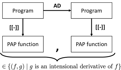
Figure 1: Lee et al. (2020)’s denotational characterization of AD, which we extend. For a simple differentiable programming language, they define a class of functions (PAP functions) expressive enough to interpret all programs in the language. Not all PAP functions are differentiable, but Lee et al. (2020) propose a relaxed notion of derivatives, called intensional derivatives, that always exist for PAP functions, and show that AD yields intensional derivatives. We extend their argument to handle recursion and higher-order functions, by defining a generalized class of $\omega$PAP functions and a corresponding generalization of the notion of intensional derivative.

The PAP functions are those with analytic piecewise representations:

Definition. If the Taylor series of a smooth function $f$ converges pointwise to $f$ in a neighborhood around $x$, we say $f$ is analytic at $x$. An analytic function is analytic everywhere in its domain. We call a set $A\subseteq\mathbb{R}^{n}$ an analytic set iff there exist finite collections $\{g^{+}_{i}\}_{i\in I}$ and $\{g^{-}_{j}\}_{j\in J}$ of analytic functions into $\mathbb{R}$, with open domains $X^{+}_{i}$ and $X^{-}_{j}$, such that $A=\{x\in(\bigcap_{i}X^{+}_{i})\cap(\bigcap_{j}X^{-}_{j})\mid\forall i.g^{+}_{i}(x)>0\wedge\forall j.g^{-}_{j}\leq 0\}$ (i.e., analytic sets are subsets of open sets carved out using a finite number of analytic inequalities.)

Definition. We say $f$ is piecewise analytic under analytic partition (PAP) if there exists a piecewise representation $\{(A_{i},f_{i})\}_{i\in I}$ of $f$ such that the $A_{i}$ are analytic sets and the $f_{i}$ are analytic functions. We call such a representation a PAP representation.

Proposition (Lee et al. 2020). Constant functions and projection functions are PAP. Supposing $f:\mathbb{R}^{n}\rightarrow\mathbb{R}$ is PAP, and $\llbracket e_{1}\rrbracket,\dots,\llbracket e_{n}\rrbracket$ are all PAP, $\llbracket f(e_{1},\dots,e_{n})\rrbracket$ and $\llbracket\texttt{if }(e_{1}>0)\,e_{2}\,e_{3}\rrbracket$ are also PAP. Therefore, by induction, all expressions $e$ denote PAP functions $\llbracket e\rrbracket$.

PAP functions are not necessarily differentiable. But Lee et al. (2020) define intensional derivatives, which do always exist for PAP functions (though unlike traditional derivatives, they are not unique):

Definition. A function $g$ is an intensional derivative of a PAP function $f$ if there exists a PAP representation $\{(A_{i},f_{i})\}_{i\in I}$ of $f$ such that when $x\in A_{i}$, $g(x)=f_{i}^{\prime}(x)$.

Lee et al. (2020) then give a standard AD algorithm for their language and show that, when applied to an expression $e$, it is guaranteed to yield some intensional derivative of $\llbracket e\rrbracket$ as long as each primitive $f$ comes equipped with an intensional derivative. Essentially, this proof is based on an analogue to the chain rule for intensional derivatives. The result is depicted schematically in Figure 1.

2.2 Challenges: Partiality, Higher-Order Functions, and Recursion

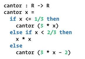
Figure 2: This program can be seen as a piecewise function, constantly $\bot$ on the $\frac{1}{3}$-Cantor set and $x^{2}$ elsewhere in $(0,1)$. But the $\frac{1}{3}$-Cantor set is not expressible as a countable union of analytic sets, and so this representation is not PAP.

Can a similar analysis be carried out for a more complex language, with higher-order and recursive functions? One challenge is that as defined above, only total, first-order functions can be PAP: unless we can generalize the definition to cover partial and higher-order functions, we cannot reproduce the inductive proof that PAP functions are closed under the programming language’s constructs. This is a roadblock even if we care only about differentiating first-order, total programs. To see why, recall that we required primitives $f$ to be PAP in the section above. What alternative requirements should we place on partial or higher-order primitives, to ensure that first-order programs built from them will be PAP? How should these primitives’ built-in intensional derivatives behave?

These are non-trivial challenges, and it is possible to formulate reasonable-sounding solutions that turn out not to work. For example, we might hypothesize that partial functions $f:U\rightharpoonup V$ definable using recursion are almost PAP: perhaps there still exists an analytic partition $\{A_{i}\}_{i\in I}$ of $U$, and analytic functions $\{f_{j}\}_{j\in J}$ for some subset of indices $J\subseteq I$, such that $f$ is defined exactly on $\bigcup_{j\in J}A_{j}$ and $f(x)=f_{j}(x)$ whenever $x\in A_{j}$. But consider the program cantor in Figure 2. It denotes a partial function that is undefined outside of $[0,1]$, and also on the $\frac{1}{3}$-Cantor set. This region cannot be expressed as a countable union of analytic sets $\cup_{i\in I\setminus J}A_{i}$. Therefore, this candidate notion of PAP partial function is too restrictive: some recursive programs do not satisfy it.

3 $\omega$PAP Semantics

In this section, we present an expressive differentiable programming language, with higher-order functions, branching, and general recursion. We then generalize the definitions of PAP functions and intensional derivatives to include higher-order and partial functions, and show that: (1) all programs in our language denote (this generalized variant of) PAP functions, and (2) a standard forward-mode AD algorithm computes valid intensional derivatives.

3.1 A Higher-Order, Recursive Differentiable Language

Syntax. Consider a language with types $\tau::=\mathbb{R}^{k}\mid\tau_{1}\times\tau_{2}\mid\tau_{1}\rightarrow\tau_{2}$, and terms $e::=x\mid c\mid e_{1}\,e_{2}\mid\texttt{if }(e_{1}>0)\,e_{2}\,e_{3}\mid\lambda x:\tau.e\mid\mu f:\tau_{1}\rightarrow\tau_{2}.e$. Here, $c$ ranges over constants of any type, including constant numeric literals such as 3 and $\pi$, as well as primitive functions such as + and sin. We write $(e_{1},e_{2})$ as sugar for $\texttt{pair}_{\tau_{1},\tau_{2}}\,e_{1}\,e_{2}$, where $\texttt{pair}_{\tau_{1},\tau_{2}}:\tau_{1}\rightarrow\tau_{2}\rightarrow\tau_{1}\times\tau_{2}$ is a constant for constructing tuples. The $\mu$ expression creates a recursive function of type $\tau_{1}\rightarrow\tau_{2}$, binding the name $f$ for the recursive call. For example, a version of the factorial function that works on natural number inputs is $\mu f:\mathbb{R}\rightarrow\mathbb{R}.(\lambda x:\mathbb{R}.\texttt{if }(x>0)\,\,(x*f(x-1))\,\,1)$.

Semantics of types. For each type $\tau$ we choose a set $\llbracket\tau\rrbracket$ of values. We have $\llbracket\mathbb{R}^{k}\rrbracket=\mathbb{R}^{k}$ and $\llbracket\tau_{1}\times\tau_{2}\rrbracket=\llbracket\tau_{1}\rrbracket\times\llbracket\tau_{2}\rrbracket$. Function types are slightly more complicated because we wish to represent partial functions. Given a set $X$, we define $X_{\bot}=\{\uparrow x\mid x\in X\}\cup\{\bot\}$. (The tag $\uparrow$ is useful to avoid ambiguity when $\bot$ is already a member of $X$: then $X_{\bot}$ contains as distinct elements the newly adjoined $\bot$ and the representation $\uparrow\bot$ of the original $\bot$ from $X$.) Using this construction, we define $\llbracket\tau_{1}\rightarrow\tau_{2}\rrbracket=\llbracket\tau_{1}\rrbracket\rightarrow\llbracket\tau_{2}\rrbracket_{\bot}$: we represent partial functions returning $\tau_{2}$ as total functions into $\llbracket\tau_{2}\rrbracket_{\bot}$.

Semantics of terms. We interpret expressions of type $\tau$ as functions from environments $\gamma$ (mapping variables $x$ to their values $\gamma[x]$) to $\llbracket\tau\rrbracket_{\bot}$. If $a\in\llbracket\tau\rrbracket_{\bot}$ and $b\in\llbracket\tau\rightarrow\sigma\rrbracket$, we write (as a mathematical expression, not an object language expression) $a\texttt{>>=}b$ to mean $\bot$ if $a=\bot$, and $b(x)$ if $a=\,\uparrow x$. Using this notation, we can define the interpretation of each construct in our language. We define: $\llbracket c\rrbracket\gamma=\uparrow c$, $\llbracket x\rrbracket\gamma=\uparrow(\gamma[x])$, $\llbracket e_{1}\,e_{2}\rrbracket\gamma=(\llbracket e_{1}\rrbracket\gamma)\texttt{>>=}(\lambda f.\llbracket e_{2}\rrbracket\gamma\texttt{>>=}f)$, $\llbracket\lambda x.e\rrbracket\gamma=\uparrow\lambda v.\llbracket e\rrbracket(\gamma[x\mapsto v])$, and $\llbracket\texttt{if }(e_{1}>0)\,e_{2}\,e_{3}\rrbracket\gamma=\llbracket e_{1}\rrbracket\gamma\texttt{>>=}\lambda x.[x>0\mapsto\llbracket e_{2}\rrbracket\gamma,x\leq 0\mapsto\llbracket e_{3}\rrbracket\gamma]$. To interpret recursion, we use the standard domain-theoretic approach. We first define partial orders $\preceq_{\tau}$ inductively for each type $\tau$: we define $x\preceq_{\mathbb{R}^{k}}y\iff x=y$, $(x_{1},x_{2})\preceq_{\tau_{1}\times\tau_{2}}(y_{1},y_{2})\iff x_{1}\preceq_{\tau_{1}}y_{1}\wedge x_{2}\preceq_{\tau_{2}}y_{2}$, and $f\preceq_{\tau\rightarrow\sigma}g\iff\forall x\in\llbracket\tau\rrbracket,f(x)\preceq^{\bot}_{\sigma}g(x)$. (The relation $x\preceq^{\bot}_{\tau}y$ holds when $x=\bot$ or when $x=\uparrow a$, $y=\uparrow b$, and $a\preceq_{\tau}b$ for some $a,b\in\llbracket\tau\rrbracket$.) Intuitively, $x\preceq y$ if $y$ is “at least as defined” as $x$. For the types $\tau$ in our language, given an infinite non-decreasing sequence $x_{1}\preceq_{\tau}x_{2}\preceq_{\tau}\dots$ of values, there exists a least upper bound $\vee_{i\in\mathbb{N}}x_{i}$. If the primitives in our language are Scott-continuous (monotone with respect to $\preceq$, with the property that $\bigvee_{i}f(x_{i})=f(\bigvee_{i}x_{i})$), we can interpret recursion: $\llbracket\mu f:\tau\rightarrow\sigma.\lambda x.e\rrbracket\gamma=\uparrow\bigvee_{i\in\mathbb{N}}f_{i}$, where $f_{0}=\lambda x.\bot$ and $f_{i}=\lambda v.\llbracket e\rrbracket(\gamma[x\mapsto v,f\mapsto f_{i-1}])$.

3.2 $\omega$PAP functions

We have given a standard denotational semantics to our language, interpreting terms as partial functions. We now generalize the notion of a PAP function to that of an $\omega$PAP partial function, and show that if all the primitives are $\omega$PAP, so is any program. The definition relies on the choice, for each type $\tau$, of a set of well-behaved or “PAP-like” functions from Euclidean space into $\llbracket\tau\rrbracket$, called the $\omega$PAP diffeology of $\tau$, by analogy with diffeological spaces (Iglesias-Zemmour, 2013).

Definition. A set $U\subseteq\mathbb{R}^{n}$ is c-analytic if it is a countable union of analytic sets.

Definition. Let $\tau$ be a type. An $\omega$PAP diffeology $\mathcal{P}_{\tau}$ for $\tau$ assigns to each c-analytic set $U$ a set $\mathcal{P}^{U}_{\tau}$ of PAP plots in $\tau$, functions from $U$ into $\llbracket\tau\rrbracket$ satisfying the following closure properties:

• (Constants.) All constant functions are plots in $\tau$.

• (Closure under PAP precomposition.) If $V\subseteq\mathbb{R}^{m}$ is a c-analytic set, and $f:V\rightarrow U$ is PAP, then $\phi\circ f$ is a plot in $\tau$ if $\phi:U\rightarrow\llbracket\tau\rrbracket$ is.

• (Closure under piecewise gluing.) If $\phi:U\rightarrow\llbracket\tau\rrbracket$ is such that the restriction $\phi|_{A_{i}}:A_{i}\rightarrow\llbracket\tau\rrbracket$ is a plot in $\tau$ for each $A_{i}$ in some c-analytic partition of $U$, then $\phi$ is a plot in $\tau$.

• (Closure under least upper bounds.) Suppose $\phi_{1},\phi_{2},\dots$ is a sequence of plots in $\tau$ such that for all $x\in U$, $\phi_{i}(x)\preceq_{\tau}\phi_{i+1}(x)$. Then $\bigvee_{i\in\mathbb{N}}\phi_{i}=\lambda x.\bigvee_{i\in\mathbb{N}}\phi_{i}(x)$ is a plot.

Choosing $\omega$PAP diffeologies. We set $\mathcal{P}^{U}_{\mathbb{R}^{k}}$ to be all PAP functions from $U$ to $\mathbb{R}^{k}$. (These trivially satisfy condition 4 above, since $\preceq_{\mathbb{R}^{k}}$ only relates equal vectors.) For $\tau_{1}\times\tau_{2}$, we include $f\in\mathcal{P}^{U}_{\tau_{1}\times\tau_{2}}$ iff $f\circ\pi_{1}\in\mathcal{P}^{U}_{\tau_{1}}$ and $f\circ\pi_{2}\in\mathcal{P}^{U}_{\tau_{2}}$. Function types are more interesting. A function $f:U\rightarrow\llbracket\tau_{1}\rightarrow\tau_{2}\rrbracket$ is a plot if, for all PAP functions $\phi_{1}:V\rightarrow U$ and plots $\phi_{2}\in\mathcal{P}^{V}_{\tau_{1}}$, the function $\lambda v.f(\phi_{1}(v))(\phi_{2}(v))$ is defined (i.e., not $\bot$) on a c-analytic subset of $V$, restricted to which it is a plot in $\tau_{2}$.

Definition. Let $\tau_{1}$ and $\tau_{2}$ be types. Then a partial $\omega$PAP function $f:\tau_{1}\rightarrow\tau_{2}$ is a Scott-continuous function from $\llbracket\tau_{1}\rrbracket$ to $\llbracket\tau_{2}\rrbracket_{\bot}$, such that if $\phi\in\mathcal{P}^{U}_{\tau_{1}}$, $f\circ\phi$ is defined on a c-analytic subset of $U$, restricted to which it is a plot in $\tau_{2}$. We revise our earlier interprtation of $\llbracket\tau_{1}\rightarrow\tau_{2}\rrbracket$ to include only the partial $\omega$PAP functions.

We note that under this definition, a total function $f:\mathbb{R}^{n}\rightarrow\mathbb{R}^{m}$ is $\omega$PAP if and only if it is PAP. The generalization becomes apparent only when working with function types and partiality.

Proposition. If every primitive function is $\omega$PAP, then every expression $e$ of type $\tau$ with free variables of type $\tau_{1},\dots,\tau_{n}$ denotes a partial $\omega$PAP function $f:\tau_{1}\times\dots\times\tau_{n}\rightarrow\tau$. In particular, programs that denote total functions from $\mathbb{R}^{n}$ to $\mathbb{R}^{m}$, even if they use recursion and higher-order functions internally, always denote (ordinary) PAP functions.

3.3 Automatic Differentiation

Implementation of AD. We now describe a standard forward-mode AD macro, adapted from Huot et al. (2020) and Vákár (2020). For each type $\tau$, we define a “dual number type” $\mathcal{D}\llbracket\tau\rrbracket$: $\mathcal{D}\llbracket\mathbb{R}^{k}\rrbracket=\mathbb{R}^{k}\times\mathbb{R}^{k}$, $\mathcal{D}\llbracket\tau_{1}\times\tau_{2}\rrbracket=\mathcal{D}\llbracket\tau_{1}\rrbracket\times\mathcal{D}\llbracket\tau_{2}\rrbracket$, and $\mathcal{D}\llbracket\tau_{1}\rightarrow\tau_{2}\rrbracket=\mathcal{D}\llbracket\tau_{1}\rrbracket\rightarrow\mathcal{D}\llbracket\tau_{2}\rrbracket$. The AD macro translates terms of type $\tau$ into terms of type $\mathcal{D}\llbracket\tau\rrbracket$: $\mathcal{D}\llbracket x\rrbracket=x$, $\mathcal{D}\llbracket e_{1}\,e_{2}\rrbracket=\mathcal{D}\llbracket e_{1}\rrbracket\,\,\mathcal{D}\llbracket e_{2}\rrbracket$, $\mathcal{D}\llbracket\texttt{if }(e_{1}>0)\,e_{2}\,e_{3}\rrbracket=\texttt{if }(\pi_{1}(\mathcal{D}\llbracket e_{1}\rrbracket)>0)\,\,\mathcal{D}\llbracket e_{2}\rrbracket\,\,\mathcal{D}\llbracket e_{3}\rrbracket$, $\mathcal{D}\llbracket\lambda x:\tau.e\rrbracket=\lambda x:\mathcal{D}\llbracket\tau\rrbracket.\mathcal{D}\llbracket e\rrbracket$, and $\mathcal{D}\llbracket\mu f:\tau\rightarrow\sigma.e\rrbracket=\mu f:\mathcal{D}\llbracket\tau\rrbracket\rightarrow\mathcal{D}\llbracket\sigma\rrbracket.\mathcal{D}\llbracket e\rrbracket$. Constants $c$ come equipped with their own translations $c_{\mathcal{D}}$: $\mathcal{D}\llbracket c\rrbracket=c_{\mathcal{D}}$. For constants of type $\mathbb{R}^{k}$, $c_{\mathcal{D}}=(c,\mathbf{0})$, but for functions, $c_{\mathcal{D}}$ encodes a primitive’s intensional derivative. For example, when $c:\mathbb{R}\rightarrow\mathbb{R}$, we require that $c_{\mathcal{D}}:\mathbb{R}\times\mathbb{R}\rightarrow\mathbb{R}\times\mathbb{R}$ be such that, for any PAP function $f:\mathbb{R}\rightarrow\mathbb{R}$ with intensional derivative $g$, there is an intensional derivative $h$ of $c\circ f$ such that $c_{\mathcal{D}}\circ\langle f,g\rangle=\lambda x.((c\circ f)(x),h(x))$. The constant log, for example, could have $\texttt{log}_{\mathcal{D}}((x,v))=(\log x,\frac{v}{x})$.

Behavior / Correctness of AD. For each type $\tau$, we define a family of relations $S^{U}_{\tau}\subseteq\mathcal{P}^{U}_{\tau}\times\mathcal{P}^{U}_{\mathcal{D}\llbracket\tau\rrbracket}$, indexed by the c-analytic sets $U$. The basic idea is that if $(f,g)\in S^{U}_{\tau}$, then $g$ is a correct “intensional dual number representation” of $f$. Since $S^{U}_{\tau}$ is a relation, there may be multiple such $g$’s, just as how in Lee et al. (2020)’s definition, a single PAP function may have multiple valid intensional derivatives.

For $\tau=\mathbb{R}^{k}$, we build directly on Lee et al. (2020)’s notion of intensional derivative: $f$ and $g$ are related in $S^{U}_{\mathbb{R}^{k}}$ if and only if, for all PAP functions $h:V\rightarrow U$ and intensional derivatives $h^{\prime}$ of $h$, there is some intensional derivative $G$ of $f\circ h$ such that for all $v\in V$, $g((h(v),h^{\prime}(v)))=((f\circ h)(v),G(v))$. For other types, we use the Artin gluing approach of Vákár (2020) to derive canonical definitions of $S_{\tau}$ for products and function types that make the following result possible:

Proposition. Suppose $(\phi,\phi^{\prime})\in S^{U}_{\tau}$, and that $e:\sigma$ has a single free variable $x:\tau$. Then $(\llbracket e\rrbracket\circ\phi,\llbracket\mathcal{D}\llbracket e\rrbracket\rrbracket\circ\phi^{\prime})$ is defined on the same c-analytic subset $V\subseteq U$, and restricted to $V$, is in $S^{V}_{\sigma}$.

Specializing to the case where $\tau$ and $\sigma$ are $\mathbb{R}^{n}$ and $\mathbb{R}^{m}$, this implies that AD gives sound intensional derivatives even when programs use recursion and higher-order functions. Intensional derivatives agree with derivatives almost everywhere, so this implies the result of Mazza and Pagani (2021).

4 Applications to Probabilistic Programming

In this section, we briefly describe some applications of the $\omega$PAP semantics to probabilistic languages. First, we give an example of applying our framework to reason about soundness for AD-powered PPL features. Second, we recover a recent result of Mak et al. (2021) via a novel denotational argument.

AD for sound change-of-variables corrections. Consider a PPL that represents primitive distributions by a pair of a sampler $\mu$ and a density $\rho$. Some systems support automatically generating a new sampler and density, $f_{*}\mu$ and $\rho_{f}$, for the pushforward of $\mu$ by a user-specified deterministic bijection $f$. Such systems compute the density $\rho_{f}$ using a change-of-variables formula, which relies on $f$’s Jacobian (Radul and Alexeev, 2021). We show in Appendix A.2 that such algorithms are sound even when: (1) $f$ is not differentiable, but rather PAP; and (2) we use not $f$’s Jacobian but any intensional Jacobian of $f$. This may be surprising, because intensional Jacobians can disagree with true Jacobians on Lebesgue-measure-zero sets of inputs, and the support of $\mu$ may lie entirely within such a set. Indeed, there are samplers $\mu$ and programs $f$ for which AD’s Jacobians are wrong everywhere within $\mu$’s support. Our result shows that this does not matter: intensional Jacobians are “wrong in the right ways,” yielding correct densities $\rho_{f}$ even when the derivatives themselves are incorrect.

Trace densities of probabilistic programs are $\omega$PAP. Now consider extending our language with constructs for probabilistic programming: a type $\mathcal{M}\,\tau$ of $\tau$-valued probabilistic programs, and constructs $\mathbf{return}_{\tau}:\tau\rightarrow\mathcal{M}\,\tau$, $\mathbf{sample}:\mathcal{M}\mathbb{R}$, $\mathbf{score}:[0,\infty)\rightarrow\mathcal{M}\,\mathbf{1}$, and $\mathbf{do}\,\{x\leftarrow t;s\}:\mathcal{M}\,\sigma$ (where $t:\mathcal{M}\,\tau$ and $s:\mathcal{M}\,\sigma$ in environments with $x:\tau$). Some PPLs use probabilistic programs only to specify density functions, for downstream use by inference algorithms like Hamiltonian Monte Carlo. To reason about such languages, we can interpret $\mathcal{M}\,\tau$ as comprising deterministic functions computing values and densities of traces. More precisely, let $\llbracket\mathcal{M}\,\tau\rrbracket=\llbracket\sqcup_{i\in\mathbb{N}}\mathbb{R}^{i}\rightarrow\textbf{Maybe }\tau\times\mathbb{R}\times\sqcup_{i\in\mathbb{N}}\mathbb{R}^{i}\rrbracket$: the meaning of a probabilistic program is a function mapping lists of real-valued random samples, called traces, to: (1) the output values they possibly induce in $\llbracket\tau\rrbracket$, (2) a density in $[0,\infty)$, and (3) a remainder of the trace, containing any samples not yet used. We can then define $\llbracket\textbf{return}_{\tau}\rrbracket=\llbracket\lambda x.\lambda\textit{trace}.(\textbf{Just }x,1.0,\textit{trace})\rrbracket$, $\llbracket\textbf{sample}\rrbracket=\llbracket\lambda\textit{trace}.(\texttt{head}\,\textit{trace},\texttt{if }(\texttt{length }\textit{trace}>0)\,(1.0)\,(0.0),\texttt{tail}\,\textit{trace})\rrbracket$, $\llbracket\textbf{score}\rrbracket=\llbracket\lambda w.\lambda\textit{trace}.(\textbf{Just }\,\langle\rangle,w,\textit{trace})\rrbracket$, and $\llbracket\textbf{do }\{x\leftarrow t;s\}\rrbracket=\llbracket\lambda\textit{trace}.\textbf{let }(x_{?},w,r)=t\,\textit{trace}\textbf{ in }\texttt{case}_{\textbf{Maybe}}\,x_{?}\,(\textbf{Nothing},0.0,\textit{trace})\,(\lambda x.\textbf{ let }(y_{?},v,u)=(s)\,r\,\textbf{ in }(y_{?},w*v,u))\rrbracket$.

Let $e:\mathcal{M}\,\tau$ be a closed probabilistic program. Suppose that on all but a Lebesgue-measure-zero set of traces, $\llbracket e\rrbracket(\textit{trace})$ is defined (i.e., not $\bot$—although the first component of the tuple it returns may be Nothing, e.g. if the input trace does not provide enough randomness to simulate the entire program). On traces where $\llbracket e\rrbracket$ is defined, the following density function is also defined: $\llbracket\lambda\textit{trace}.\textbf{let }\,(x_{?},w,r)=e\,\textit{trace}\textbf{ in if }(\texttt{length }\,r>0)\,\,(0.0)\,\,(w)\rrbracket$. Furthermore, as a function in the language, this density function is $\omega$PAP. Therefore, excepting the measure-zero set on which it is undefined, for each trace length, the density function is PAP in the ordinary sense—and therefore almost-everywhere differentiable. This result was recently proved using an operational semantics argument by Mak et al. (2021). The PAP perspective helps reason denotationally about such questions, and validates that AD on trace density functions in PPLs produces a.e.-correct derivatives.

Future work. Besides the “trace-based” approach described above, we are working on an extensional monad of measures similar to that of Vákár et al. (2019), but in the $\omega$PAP category. This could yield a semantics in which results from measure theory and the differential calculus can be combined, to establish the correctness of AD-powered PPL features like automated involutive MCMC (Cusumano-Towner et al., 2020). However, more work may be needed to account for the variational inference, which uses gradients of expectations. In our current formulation of the measure monad, the real expectation operator $\mathbb{E}_{\mathbb{R}}:\mathcal{M\,\tau}\rightarrow(\tau\rightarrow\mathbb{R})\rightarrow\mathbb{R}$ is not $\omega$PAP, and so we cannot reason in general about when the expectation of an $\omega$PAP function under a probabilistic program will be differentiable.

Appendix A Appendix

A.1 Type system of the language

Figure 3 shows the type system of our language from Section 3; all rules are standard.

$\Gamma\vdash x:\tau$

$(x:\tau\in\Gamma)$   $\Gamma\vdash c:\tau$ $(c\in\mathcal{C}_{\tau})$   $\Gamma,x:\tau_{1}\vdash e:\tau_{2}$ $\Gamma\vdash\lambda x:\tau_{1}.e:\tau_{1}\to\tau_{2}$

$\Gamma\vdash e_{1}:\tau_{1}\to\tau_{2}$  $\Gamma\vdash e_{2}:\tau_{1}$

$\Gamma\vdash e_{1}e_{2}:\tau_{2}$

$\Gamma\vdash e_{1}:\mathbb{R}$  $\Gamma\vdash e_{2}:\tau$  $\Gamma\vdash e_{3}:\tau$

$\Gamma\vdash\texttt{if}\,(e_{1}>0)\,e_{2}\,e_{3}:\tau$

$\Gamma,f:\tau_{1}\to\tau_{2}\vdash e:\tau_{1}\to\tau_{2}$

$\Gamma\vdash\mu f:\tau_{1}\to\tau_{2}.e:\tau_{1}\to\tau_{2}$

Figure 3: Type system of our language.

A.2 Argument for the soundness of change-of-variables calculations with intensional derivatives

Let $\mu$ be a probability distribution over (possibly some sub-manifold of) $\mathbb{R}^{n}$, with density $\rho$ with respect to a reference measure $B_{\mu}$. Suppose we have a “change-of-variables” algorithm that computes densities $\rho_{f}$, with respect to a reference measure $B_{f}$, of pushforwards $f_{*}\mu$ of $\mu$ by differentiable bijections $f$. The algorithm may use the true derivatives of $f$. We show that such an algorithm also works when $f$ is PAP, if it is given intensional derivatives of $f$ instead of true ones.

Let $f$ be a PAP bijection from $\mathbb{R}^{k}$ to $\mathbb{R}^{m}$ (more precisely, it need only be bijective when restricted to the support of $\mu$). Suppose $g$ is an intensional Jacobian of $f$, meaning there exists a (PAP) piecewise representation $\{A_{i},f_{i}\}_{i\in I}$ of $f$ such that $g(x)=Jf_{i}(x)$ when $x\in A_{i}$. Because the $A_{i}$ form a partition of $f$’s domain, we have $\mu=\sum_{i\in I}\mathbf{1}_{A_{i}}\odot\mu$, where $h\odot\mu$ is the measure obtained by scaling $\mu$ by a scalar function $h$. Then $f_{*}\mu=\sum_{i\in I}f_{*}(\mathbf{1}_{A_{i}}\odot\mu)=\sum_{i\in I}(f_{i})_{*}(\mathbf{1}_{A_{i}}\odot\mu)$. For each $i\in I$, suppose $\rho_{f,i}$ is a density of $(f_{i})_{*}(\mathbf{1}_{A_{i}}\odot\mu)$ with respect to $B_{f}$. At points in $A_{i}$, such densities are soundly computed using the original change-of-variables algorithm, because $f_{i}$ is differentiable and $g$ gives its (ordinary) Jacobian. Summing these densities (only one of which is non-zero at each point $x$) gives a density $\rho_{f}$ of $f_{*}\mu$.

References

- Abadi and Plotkin [2020] Martín Abadi and Gordon D Plotkin. A simple differentiable programming language. In Proc. POPL 2020. ACM, 2020.
- Bingham et al. [2019] Eli Bingham, Jonathan P Chen, Martin Jankowiak, Fritz Obermeyer, Neeraj Pradhan, Theofanis Karaletsos, Rohit Singh, Paul Szerlip, Paul Horsfall, and Noah D Goodman. Pyro: Deep universal probabilistic programming. The Journal of Machine Learning Research, 20(1):973–978, 2019.
- Cusumano-Towner et al. [2020] Marco Cusumano-Towner, Alexander K Lew, and Vikash K Mansinghka. Automating involutive mcmc using probabilistic and differentiable programming. arXiv preprint arXiv:2007.09871, 2020.
- Cusumano-Towner et al. [2019] Marco F Cusumano-Towner, Feras A Saad, Alexander K Lew, and Vikash K Mansinghka. Gen: a general-purpose probabilistic programming system with programmable inference. In Proceedings of the 40th acm sigplan conference on programming language design and implementation, pages 221–236, 2019.
- Goodman et al. [2012] Noah Goodman, Vikash Mansinghka, Daniel M Roy, Keith Bonawitz, and Joshua B Tenenbaum. Church: a language for generative models. arXiv preprint arXiv:1206.3255, 2012.
- Huot et al. [2020] Mathieu Huot, Sam Staton, and Matthijs Vákár. Correctness of automatic differentiation via diffeologies and categorical gluing. arXiv preprint arXiv:2001.02209, 2020.
- Iglesias-Zemmour [2013] Patrick Iglesias-Zemmour. Diffeology, volume 185. American Mathematical Soc., 2013.
- Lee et al. [2020] Wonyeol Lee, Hangyeol Yu, Xavier Rival, and Hongseok Yang. On correctness of automatic differentiation for non-differentiable functions. arXiv preprint arXiv:2006.06903, 2020.
- Mak et al. [2021] Carol Mak, C-H Luke Ong, Hugo Paquet, and Dominik Wagner. Densities of almost surely terminating probabilistic programs are differentiable almost everywhere. Programming Languages and Systems, 12648:432, 2021.
- Mazza and Pagani [2021] Damiano Mazza and Michele Pagani. Automatic differentiation in pcf. Proceedings of the ACM on Programming Languages, 5(POPL):1–27, 2021.
- Radul and Alexeev [2021] Alexey Radul and Boris Alexeev. The base measure problem and its solution. In International Conference on Artificial Intelligence and Statistics, pages 3583–3591. PMLR, 2021.
- Vákár [2020] Matthijs Vákár. Denotational correctness of foward-mode automatic differentiation for iteration and recursion. arXiv preprint arXiv:2007.05282, 2020.
- Vákár et al. [2019] Matthijs Vákár, Ohad Kammar, and Sam Staton. A domain theory for statistical probabilistic programming. Proceedings of the ACM on Programming Languages, 3(POPL):36, 2019.