Boosting Discriminative Visual Representation Learning with Scenario-Agnostic Mixup

Abstract

Mixup is a well-known data-dependent augmentation technique for DNNs, consisting of two sub-tasks: mixup generation and classification. However, the recent dominant online training method confines mixup to supervised learning (SL), and the objective of the generation sub-task is limited to selected sample pairs instead of the whole data manifold, which might cause trivial solutions. To overcome such limitations, we comprehensively study the objective of mixup generation and propose Scenario-Agnostic Mixup (SAMix) for both SL and Self-supervised Learning (SSL) scenarios. Specifically, we hypothesize and verify the objective function of mixup generation as optimizing local smoothness between two mixed classes subject to global discrimination from other classes. Accordingly, we propose $\eta$-balanced mixup loss for complementary learning of the two sub-objectives. Meanwhile, a label-free generation sub-network is designed, which effectively provides non-trivial mixup samples and improves transferable abilities. Moreover, to reduce the computational cost of online training, we further introduce a pre-trained version, SAMix^P, achieving more favorable efficiency and generalizability. Extensive experiments on nine SL and SSL benchmarks demonstrate the consistent superiority and versatility of SAMix compared with existing methods.

1 Introduction

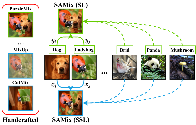
Figure 1: Illustration of SAMix. Labels are required for the mixed samples in green boxes but not for the blue ones. The solid line indicates that the local relationship directly influences the mixed sample, whereas the dashed one denotes that samples of the other classes serve as global constraints on the current mixed data. Compared to handcrafted policies focusing only on local sample pairs, SAMix can exploit local and global information for mixup generation while exerting no dependency on labels.

One of the fundamental problems in machine learning is how to learn a proper low-dimensional representation that captures intrinsic data structures and facilitates downstream tasks in an efficient manner [1, 2, 3, 4]. Data mixing, as a means of generating symmetric mixed data and labels, has largely improved the efficiency of deep neural networks (DNNs) in learning discriminative representation across various scenarios [5, 6, 7], especially for Vision Transformers (ViTs) [8, 9]. Despite its general application, the policy of sample generation process in data mixing requires an explicit design (e.g. linear interpolation or random local patch replacement). Differ from that, the optimizable data mixing algorithms utilize labels to localize task-relevant targets (e.g., gradCAM [10]) and thereby generate semantic mixed samples such as offline maximizing saliency information of related samples [6, 11, 12]. These handcrafted mixing policies are shown in the red box of Figure 1. Additionally, [13] learns a mixup generator by supervised adversarial training.

Most current works combine mixup with contrastive learning, which directly transfers linear mixup methods into contrastive learning [7, 14, 15]. The recently proposed AutoMix [16] provides a novel perspective to make mixup policy parameterized and can be trained online. Although these optimizable methods have attained significant gains in supervised learning (SL) tasks, they still do not exploit the underlying structure of the whole observed data manifold, resulting in trivial solutions without the guidance of labels, which makes them fail to apply in self-supervised learning (SSL) scenarios (discussed in Section 2). The question then naturally arises as to whether it is possible to design a more generalized and trained mixup policy that can be applied to both SL and SSL scenarios. To achieve this goal, there are two remaining open challenges to be solved: (i) how to solve the problem of trivial solutions in online training approaches; (ii) how to design a proper generation objective to make the algorithm generalizable for both SL and SSL.

In this paper, we propose Scenario-Agnostic Mixup (SAMix), a framework shown in Figure 1 that employs $\eta$-balanced mixup loss (Section 3.1) for treating mixup generation and classification differently from a local and global perspective. At the same time, specially designed Mixer (Section 3.2) generate mixed samples adaptively either at instance-level or cluster-level to tackle the trivial solutions effectively. Furthermore, in order to eliminate the drawback of poor versatility and computational overhead in SAMix optimization, we propose a pre-trained setting, SAMix^P, which employs a pre-trained Mixer to generate high-quality mixed samples balancing performance and speed for various downstream applications. Noticed that SAMix^P can achieve competitive or slightly higher performances than SAMix in classification tasks. Comprehensive experiments demonstrate the effectiveness and transferring abilities of SAMix. Our contributions are summarized as follows:

• We decompose mixup learning objectives into local and global terms and further analyze the corresponding properties (local smoothness and global discrimination) of mixup generation, then design $\eta$-balanced loss to targetedly boost mixup generation performance.

• We build a label-free mixup generator, Mixer, with mixing attention and non-linear content modeling which effectively tackles the trivial solution problem in existing learnable methods and thus makes it more adaptive and transferable for varied scenarios.

• Combining the above $\eta$-balanced loss and specially tailored label-free Mixer, a unified scenario-agnostic mixup training framework, SAMix, is proposed that supports online and pre-trained pipelines for both SL and SSL tasks.

• Built on SAMix framework, a pre-trained version named SAMix^P is provided, which brings SAMix more favorable performance-efficiency trade-offs and generalizability across multifarious visual downstream tasks.

2 Preliminaries

Given a finite set of i.i.d samples, $X=[x_{i}]_{i=1}^{n}\in\mathbb{R}^{D\times n}$, each data $x_{i}\in\mathbb{R}^{D}$ is drawn from a mixture of, say $C$, distributions $\mathcal{D}=\{\mathcal{D}_{c}\}_{c=1}^{C}$. Our basic assumption for discriminative representations is that the each component distribution $\mathcal{D}_{c}$ has relatively low-dimensional intrinsic structures, i.e., the distribution $\mathcal{D}_{c}$ is constrained on a sub-manifold, say $\mathcal{M}_{c}$ with dimension $d_{c}\ll D$. The distribution $\mathcal{D}$ of $X$ is consisted of sub-manifolds, $\mathcal{M}=\cup_{c=1}^{C}\mathcal{M}_{c}$. We seek a low-dimensional representation $z_{i}\in\mathcal{M}$ of $x_{i}$ by learning a continuous mapping by a network encoder, $f_{\theta}(x):x\longmapsto z$ with the parameter $\theta\in\Theta$, which captures intrinsic structures of $\mathcal{M}$ and facilitates the discriminative tasks.

2.1 Discriminative Representation Learning

Parametric training with class supervision. Some supervised class information is available to ease the discriminative tasks in practical scenarios. Here, we assume that a one-hot label $y_{i}\in\mathbb{R}^{C}$ of each sample $x_{i}$ can be somehow obtained, $Y=[y_{1},y_{2},...,y_{n}]\in\mathbb{R}^{C\times n}$. We denote the labels generated during training as pseudo labels (PL), while the fixed as ground truth labels (L). Notice that each component $\mathcal{D}_{c}$ is considered separated according to $Y$ in this scenario. Then, a parametric classifier, $g_{\omega}(z):z\longmapsto p$ with the parameter $\omega\in\Omega$, can be learned to map the representation $z_{i}$ of each sample to its class label $y_{i}$ by predicting the probability of $p_{i}$ being assigned to the $c$-th class using the softmax criterion, $p_{c|i}=\frac{\exp(w_{c}^{T}z_{i})}{\sum_{j=1}^{C}\exp(w_{j}^{T}z_{i})}$, where $w_{c}$ is a weight vector for the class $c$, and $w_{c}^{T}z_{i}$ measures how similar between $z_{i}$ and the class $c$. The learning objective is to minimize the cross-entropy loss (CE) between $y_{i}$ and $p_{i}$,

$$\vspace{-1pt}\ell^{\,CE}(y_{i},p_{i})=-y_{i}\log p_{i}.\vspace{-1pt}$$ (1)

Non-parametric training as instance discrimination. Complementary to the above parametric settings, non-parametric approaches are usually adopted in unsupervised scenarios. Due to the lack of class information, an instance discriminative task can be designed based on an assumption of local compactness. We mainly discuss contrastive learning (CL) and take MoCo [17] as an example. Consider a pair of augmented image $(x_{i}^{\tau_{q}},x_{i}^{\tau_{k}})$ from the same instance $x_{i}\in\mathbb{R}^{C\times H\times W}$, the local compactness is introduced by alignment of the encoded representation pair $(z_{i}^{\tau_{q}},z_{i}^{\tau_{k}})$ from $f_{\theta,q}$ and the momentum $f_{\theta,k}$, and constrained to the global uniformity by contrasting $z_{i}^{\tau_{q}}$ to a dictionary of encoded keys from other images, $\{z_{j}^{\tau_{k}}\}_{j=1}^{K}$, where $K$ denotes the length of the dictionary. It can be achieved by the popular non-parametric CL loss with temperature $t$, called infoNCE [18]:

$$\vspace{-3pt}\ell^{\,NCE}(z_{i}^{\tau_{q}},z_{i}^{\tau_{k}})=-\log\frac{\exp(z_{i}^{\tau_{q}}z_{i}^{\tau_{k}}/t)}{\sum^{K}_{j=1}\exp(z_{i}^{\tau_{q}}z_{j}^{\tau_{k}}/t)}.\vspace{-4pt}$$ (2)

2.2 Mixup for Discriminative Representation

We further consider mixup as a generation task into discriminative representation learning to form a closed-loop framework. Then we have two mutually benefited sub-tasks: (a) mixed data generation and (b) classification. As for the sub-task (a), we define two functions, $h(\cdot)$ and $v(\cdot)$, to generate mixed samples and labels with a mixing ratio $\lambda\sim Beta(\alpha,\alpha)$. Given the mixed data, (b) defines a mixup training objective to optimize the representation space between instances or classes.

Mixup classification as the main task. Since we aim to seek a good representation to facilitate discriminative tasks, thus the mixed samples should be diverse and well-characterized. The mixed samples with semantic information can be easily obtained by parametric learning, while it becomes a challenge without supervision. Therefore, two types of the mixup classification objective $\mathcal{L}_{\theta,\omega}$ can be defined for class-level and instance-level mixup training. As for parametric training, given two randomly selected data pairs, $(x_{i},y_{i})$ and $(x_{j},y_{j})$, the mixed data is generated as $x_{m}=h(x_{i},x_{j},\lambda)$ and $y_{m}=v(y_{i},y_{j},\lambda)$. The objective of class-level mixup is similar to Eq. 1 as,

$$\ell^{\,CE}(y_{m},p_{m})=\lambda\ell^{\,CE}(y_{m},p_{m})+(1-\lambda)\ell^{\,CE}(y_{m},p_{m}).$$ (3)

Notice that we fix $v(\cdot)$ as the linear interpolation in our discussions, i.e., $v(y_{i},y_{j},\lambda)\triangleq\lambda y_{i}+(1-\lambda)y_{j}$. Symmetrically, we denote $h(\cdot)$ as a pixel-wise mixing policy with element-wise product $\odot$ for most input mixup methods [5, 19, 6], i.e., $x_{m}=s_{i}\odot x_{i}+s_{j}\odot x_{j}$, where $s_{i}\in\mathbb{R}^{H\times W}$ is a pixel-wise mask and $s_{j}=1-s_{i}$. Notice that each coordinate $s_{w,h}\in[0,1]$. We can generate $x_{m}$ with a pair of randomly selected samples $(x_{i},x_{j})$ and formulate mixup infoNCE loss for instance-level mixup:

$$\ell^{NCE}(z_{m})=\lambda\ell^{NCE}(z_{m},z_{i})+(1-\lambda)\ell^{NCE}(z_{m},z_{j}),$$ (4)

where $z_{m}$, $z_{i}$ and $z_{j}$ denote the corresponding representations. The major difference with Eq. 3 is that the augmentation view that generates $z_{m}$ is not from the same view, i.e., $z_{i}$ and $z_{j}$, as the objective function, which is effective in retaining task-relevant information, details in A.5.1.

Mixup generation as the auxiliary task. Unlike the learning object on the unmixed data $X$ in Sec. 2.1, the performance of (b) mixup classification mainly depends on the quality of (a) mixup generation. We thus regard (a) as an auxiliary task to (b) and model $h(\cdot)$ as a sub-network $\mathcal{M}_{\phi}$ with the parameter $\phi\in\Phi$, called Mixer. Specifically, (a) aims to generate a pixel-wise mask $s\in\mathbb{R}^{H\times W}$ for mixing sample pairs. The mixup mask $s_{i}$ should directly related to $\lambda$ and the contents of $(x_{i},x_{j})$. Practically, our $\mathcal{M}_{\phi}$ takes $l$-th layer feature maps $z^{l}\in\mathbb{R}^{C_{l}\times H_{l}\times W_{l}}$ and $\lambda$ value as the input, $\mathcal{M}_{\phi}:x_{i},x_{j},z_{i}^{l},z_{j}^{l},\lambda\longmapsto x_{m}$. The generation process of $\mathcal{M}_{\phi}$ can be trained by a mixup generation loss as $\mathcal{L}_{\phi}^{gen}$, and a mask loss designed for generated mask $s_{i}$ denoted as $\mathcal{L}_{\phi}^{mask}$. Formally, we have the mixup generation loss as $\mathcal{L}_{\phi}=\mathcal{L}_{\phi}^{cls}+\mathcal{L}_{\phi}^{mask}$, and the final learning objective is,

$$\mathop{\min}\limits_{\theta,\omega,\phi}\mathcal{L}_{\theta,\omega}+\mathcal{L}_{\phi}.$$ (5)

Both $\mathcal{L}_{\theta,\omega}$ and $\mathcal{L}_{\phi}$ can be optimized alternatively in a unified framework using a momentum pipeline with the stop-gradient operation [20, 16], as shown in Figure 5 (left). However, in SSL, this framework can easily make the generator fall into a trivial solution. To solve this problem, we propose a novel mixup loss function and a generator architecture, Mixer. Combining the two can fully exploit the ability of mixup in learning discriminative features.

3 SAMix for Discriminative Representations

3.1 Learning Objective for Mixup Generation

Typically the objective function $\mathcal{L}_{\phi}$ corresponding to the mixup generation is consistent with the classification in parametric training (e.g., $\ell^{CE}$). In this paper, we argue that mixup generation is aimed to optimize the local term subject to the global term. The local term focuses on the classes of sample pairs to be mixed, while the global term introduces the constraints of other classes. For example, $\ell^{CE}$ is the global term whose each class produces an equivalent effect on the final prediction without focusing on the relevant classes of the current sample pair. At the class level, to emphasize the local term, we introduce a parametric binary cross-entropy (pBCE) loss for the generation task. Formally, assuming $y_{i}$ and $y_{j}$ belong to the class $a$ and class $b$, pBCE can be summarized as:

$$\ell_{+}^{\,CE}(p_{m})=-\lambda y_{i,a}\log p_{m}-(1-\lambda)y_{j,b}\log p_{m},$$ (6)

where $y_{i,a}=1$ and $y_{i,b}=1$ denote the one-hot label for the class $a$ and $b$. Notice that we use $\ell_{+}$ and $\ell_{-}$ to represent the local and global terms, and $\ell_{-}$ for the parametric loss refers to $\ell^{\,CE}$. Symmetrically, we have non-parametric binary cross-entropy mixup loss (BCE) for CL:

$$\ell_{+}^{NCE}(z_{m})=-\lambda\log p_{m,i}-(1-\lambda)\log p_{m,j},$$ (7)

where $p_{m,i}=\frac{\exp(z_{m}z_{i}/t)}{\exp(z_{m}z_{i}/t)+\exp(z_{m}z_{j}/t)}$ and its $\ell_{-}$ refers to $\ell^{NCE}$.

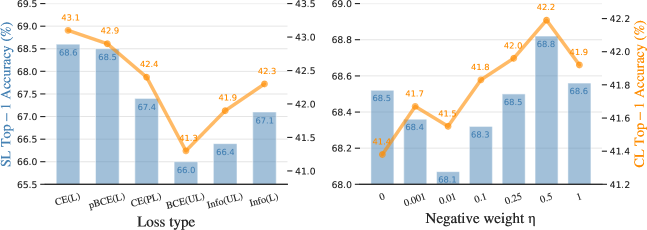
Figure 2: Analysis of the learning objective of Mixer on Tiny ImageNet with ResNet-18. The left figure shows the results of various losses on the SL task (left y axis) and the CL task (right y axis). The right one shows the effect of using various negative weights $\eta$.

Balancing local and global terms. Since both the local and global terms contribute to mixup generation, we analyze the importance of each term in both the SL and SSL tasks to design a balanced learning objective. We first analyze the properties of both terms with two hypothesizes: (i) the local term $\ell_{+}$ determines the generation performance, (ii) the global term $\ell_{-}$ improves global discrimination but is sensitive to class information. To verify these properties, we design an empirical experiment based on the proposed Mixer on Tiny (see A.5). The main difference between the mixup CE and infoNCE is whether to adopt parametric class centroids. Therefore, we compare the intensity of class information among unlabeled (UL), pseudo labels (PL), and ground truth labels (L). Notice that PL is generated by ODC [21] with the cluster number $C$. The class supervision can be imported to mixup infoNCE loss by filtering out negative samples with PL or L as [22] denoted as infoNCE (L) and infoNCE (PL). As shown in Figure 2 (left), our hypothesizes are verified in the SL task (as the performance decreases from CE(L) to pBCE(L) and CE(PL) losses), but the opposite result appears in the CL task. The performance increases from InfoNCE(UL) to InfoNCE(L) as the false negative samples are removed [23, 22] while trivial solutions occur using BCE(UL) (in Figure 6). Therefore, we propose it is better to explicitly import class information as PL for instance-level mixup to generate "strong" inter-class mixed samples while preserving intra-class compactness.

SAMix with $\eta$-balanced generation objectives. Practically, we provide two versions of the learning objective: the mixup CE loss with PL as the class-level version (SAMix-C), and the mixup infoNCE loss as the instance-level version (SAMix-I). Then, we hypothesize that the best performing mixed samples will be close to the sweet spot: achieving $\lambda$ smoothness locally between two classes or neighborhood systems while globally discriminating from other classes or instances. We propose an $\eta$-balanced mixup loss as the objective of mixup generation,

$$\ell_{\eta}=\ell_{+}+\eta\ell_{-},\ \eta\in[0,1].$$ (8)

We analyze the performance of using various $\eta$ in Eq. 8 on Tiny, as shown in Figure 2 (right), and find that using $\eta=0.5$ performs best on both the SL and CL tasks. In the end, we provide the learning objective, $\mathcal{L}_{\phi}^{cls}\triangleq\ell^{\,CE}_{+}+\eta\ell^{\,CE}_{-}$, with L for class-level mixup and with PL for SAMix-C, $\mathcal{L}_{\phi}^{cls}\triangleq\ell^{NCE}_{+}+\eta\ell^{NCE}_{-}$ for SAMix-I (details in A.2).

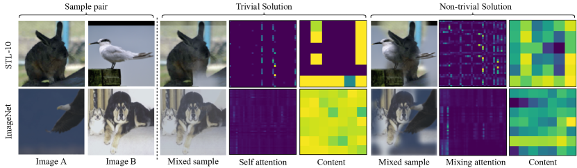
Figure 3: Visualization of trivial (using linear $\mathcal{C}$ and self-attention) and non-trivial solutions (using the proposed non-linear $\mathcal{C}_{NC}$ and mixing attention) for SAMix-I on STL-10 and IN-1k.

3.2 De Novo Mixer for Mixup Generation

Although AutoMix proposes the MixBlock that learns adaptive mixup generation policies online, there are three drawbacks in practice: (a) fail to encode the mixing ratio $\lambda$ on small datasets; (b) fall into trivial solutions when performing CL tasks; (c) the online training pipeline leads to double or more computational costs than MixUp. Our Mixer $\mathcal{M}_{\phi}$ solves these problems individually.

Adaptive $\lambda$ encoding and mixing attention. Since a randomly sampled $\lambda$ should directly guide mixup generation, the predicted mask $s$ should be semantically proportional to $\lambda$. The previous typical design regards $\lambda$ as the prior knowledge and concatenates $\lambda$ to input feature maps, which might be unable to encode $\lambda$ properly (the analysis in A.6.1). We propose an adaptive $\lambda$ encoding as,

$$z^{l}_{i,\lambda}=(1+\gamma\lambda)z_{i}^{l},$$ (9)

where $\gamma$ is a learnable scalar that constrained to $[0,1]$. Notice that $\gamma$ is initialized to $0$ during training. As shown in Figure 4, we compute the mixing relationship between two samples using a new mixing attention: we concatenate $(z^{l}_{i,\lambda},z^{l}_{j,1-\lambda})$ as the input, $\tilde{z}^{l}={\rm{concat}}(z^{l}_{i,\lambda},z^{l}_{j,1-\lambda})$, and compute the attention matrix as,

$$P_{i,j}={\psi}(\frac{(W_{P}\tilde{z}^{l})^{T}\otimes W_{P}\tilde{z}^{l}}{\mathcal{N}(\tilde{z}^{l})}),$$ (10)

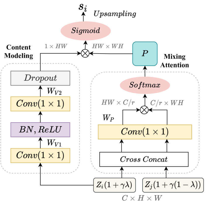
Figure 4: The network architecture of the proposed Mixer for mixup generation.

where $\psi(\cdot)$ is the softmax function, $\mathcal{N}(\tilde{z}^{l})$ denotes a normalization factor, and $\otimes$ is matrix multiplication. Notice that the mixing attention provides both the cross-attention between $z^{l}_{i,\lambda}$ and $z^{l}_{j,\lambda}$ and the self-attention of each feature itself.

Non-linear content modeling. In vanilla self-attention mechanism, the content sub-module $\mathcal{C}$ is a linear projection, $C_{i}=W_{z}\tilde{z}^{l}$, where $W_{z}$ denotes a $1\times 1$ convolution. However, we find the training process of this structure is unstable when performing CL tasks with the linear $\mathcal{C}$ in the early period and sometimes trapped in trivial solutions, such as all coordinates on $s_{i}$ predicted as a constant. As shown in Figure 3, we visualize $C_{i}$ and $P_{i,j}$ of trivial and non-trivial results, and find that the trivial $s_{i}$ is usually caused by a constant $C_{i}$. We hypothesize that trivial solutions happen earlier in the linear $\mathcal{C}$ than in $P_{i,j}$, because it might be unstable to project high-dimensional features to $1$-dim linearly. Hence, we design a non-linear content modeling sub-module $\mathcal{C}_{NC}$ that contains two $1\times 1$ convolution layers with a batch normalization layer and a ReLU layer in between, as shown in Figure 4. To increase the robustness and randomness of mixup training, we add a Dropout layer with a dropout ratio of $0.1$ in $\mathcal{C}_{NC}$. Formally, Mixer $\mathcal{M}_{\phi}$ can be written as,

$$s_{i}=U\bigg{(}\sigma\Big{(}{\psi}\big{(}\frac{(W_{P}\tilde{z}^{l})^{T}\otimes W_{P}\tilde{z}^{l}}{\mathcal{N}(\tilde{z}^{l})}\big{)}\otimes\mathcal{C}_{NC}(z^{l}_{i,\lambda})\Big{)}\bigg{)}.$$ (11)

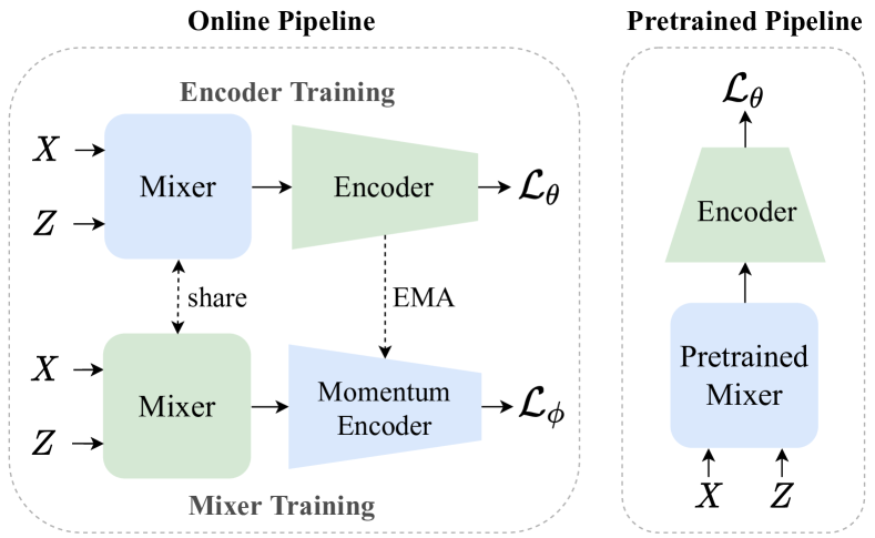
Figure 5: Training framework comparison of the online pipeline (left) in AutoMix and the proposed pre-trained pipeline (right). $X$ and $Z$ denote the input sample and corresponding feature maps from Momentum Encoder. Blue modules are not updated by back-propagation. The online pipeline optimizes Mixer and Encoder alternatively, while the pre-trained pipeline adopts pre-trained Mixer on large datasets.

Pre-trained pipeline v.s. Online pipeline. Even though online-optimized mixup methods [16] outperform their handcrafted counterparts by a substantial margin, their extra computational cost is intolerable especially for large datasets. On large-scale benchmarks, we observe that the mixed samples generated by SAMix in both early and late training periods or with different CNN encoders vary little. Consequently, we hypothesize that, similar to knowledge distillation [24], we can replace the online training Mixer in our SAMix with a pre-trained one. From this perspective, we propose the pre-trained SAMix pipeline, denoted as SAMix^P, in Figure 5. We can conclude: (i) SAMix^P pre-trained on large-scale datasets achieves similar or better performance as its online training version on current or relevant datasets with less computational cost. (ii) SAMix^P with light or median CNN encoders (e.g., ResNet-18) yields better performance than heavy ones (e.g., ResNet-101). (iii) SAMix^P has better transferring abilities than AutoMix^P. (iv) Online training pipeline is still irreplaceable on small datasets (e.g., CIFAR and CUB).

Prior knowledge of mixup. Moreover, we summarize some commonly adopted prior knowledge [6, 24] for mixup as two aspects: (a) adjusting the mean of $s_{i}$ correlated with $\lambda$, and (b) balancing the smoothness of local image patches while maintaining discrimination of $x_{m}$. Based on them, we introduce $\lambda$ adjusting and modifying the mask loss $\mathcal{L}_{\phi}^{mask}$ (details in A.2).

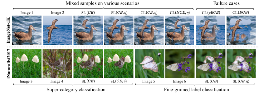
Figure 6: Visualization and comparison of mixed samples from Mixer in various learning scenarios on IN-1k and iNat2017. Note that $\lambda=0.5$ and $\eta=0.5$ if the balance coefficient $\eta$ is included. CL(C) and CL(I) denote using SAMix-C and SAMix-I separately.

3.3 Discussion and Visualization of SAMix

To show the influence of local and global constraints on mixup generation, we visualize mixed samples generated from Mixer on various scenarios in Figure 6. It is clear that SAMix captures robust underlying data structure from both class- and instance-level effectively and thus can avoid trivial solutions and then become more applicable for SSL.

Class-level. In the supervised task, global constraint localizes key features by discriminating to other classes, while the local term is prone to preserve more information related to the current two samples and classes. For example, comparing the mixed results with and without $\eta$-balanced mixup loss, it was found that pixels of the foreground target were of interest to Mixer. When the global constraint is balanced ($\eta=0.5$), the foreground target is retained more completely. Importantly, our designed Mixer remains invariant to the background for the more challenging fine-grained classification and preserves discriminative features.

Table 1: Top-1 Acc (%) of image classification on IN-1k training 100-epoch and 300-epoch using procedures.

	PyTorch 100ep					PyTorch 300ep
Methods	R-18	R-34	R-50	R-101	RX-101	R-18	R-34	R-50	R-101
Vanilla	70.04	73.85	76.83	78.18	78.71	71.83	75.29	77.35	78.91
Mixup	69.98	73.97	77.12	78.97	79.98	71.72	75.73	78.44	80.60
CutMix	68.95	73.58	77.17	78.96	80.42	71.01	75.16	78.69	80.59
ManifoldMix	69.98	73.98	77.01	79.02	79.93	71.73	75.44	78.21	80.64
SaliencyMix	69.16	73.56	77.14	79.32	80.27	70.21	75.01	78.46	80.45
FMix∗	69.96	74.08	77.19	79.09	80.06	70.30	75.12	78.51	80.20
PuzzleMix	70.12	74.26	77.54	79.43	80.63	71.64	75.84	78.86	80.67
ResizeMix∗	69.50	73.88	77.42	79.27	80.55	71.32	75.64	78.91	80.52
AutoMix	70.50	74.52	77.91	79.87	80.89	72.05	76.10	79.25	80.98
SAMixP	70.83	74.95	78.06	80.05	80.98	72.27	76.28	79.39	81.10
SAMix	70.85	74.96	78.11	80.02	81.03	72.33	76.35	79.40	81.06

Table 2: Top-1 Acc (%) of image classification on iNat2017/2018 and Places205.

	iNat2017		iNat2018		Places205
Method	R-50	RX-101	R-50	RX-101	R-18	R-50
Vanilla	60.23	63.70	62.53	66.94	59.63	63.10
Mixup	61.22	66.27	62.69	67.56	59.33	63.01
CutMix	62.34	67.59	63.91	69.75	59.21	63.75
ManifoldMix	61.47	66.08	63.46	69.30	59.46	63.23
SaliencyMix	62.51	67.20	64.27	70.01	59.50	63.33
FMix∗	61.90	66.64	63.71	69.46	59.51	63.63
PuzzleMix	62.66	67.72	64.36	70.12	59.62	63.91
ResizeMix∗	62.29	66.82	64.12	69.30	59.66	63.88
AutoMix∗	63.08	68.03	64.73	70.49	59.74	64.06
SAMixP	63.38	68.23	65.16	70.56	59.82	64.35
SAMix	63.32	68.26	64.84	70.54	59.86	64.27

Table 3: Top-1 Acc (%) of supervised image classification on CIFAR-100, Tiny-ImageNet, CUB-200 and Aircraft.

	CIFAR-100			Tiny-ImageNet		CUB-200		FGVC-Aircraft
Method	R-18	RX-50	WRN-28-8	R-18	RX-50	R-18	RX-50	R-18	RX-50
Vanilla	78.04	81.09	81.63	61.68	65.04	77.68	83.01	80.23	85.10
Mixup	79.12	82.10	82.82	63.86	66.36	78.39	84.58	79.52	85.18
CutMix	78.17	81.67	84.45	65.53	66.47	78.40	85.68	78.84	84.55
ManifoldMix	80.35	82.88	83.24	64.15	67.30	79.76	86.38	80.68	86.60
SaliencyMix	79.12	81.53	84.35	64.60	66.55	77.95	83.29	80.02	84.31
FMix∗	79.69	81.90	84.21	63.47	65.08	77.28	84.06	79.36	84.85
PuzzleMix	80.43	82.57	85.02	65.81	66.92	78.63	84.51	80.76	86.23
ResizeMix∗	80.01	81.82	84.87	63.74	65.87	78.50	84.77	78.10	84.08
AutoMix∗	82.04	83.64	85.16	67.33	70.72	79.87	86.56	81.37	86.69
SAMix	82.30	84.42	85.50	68.89	72.18	81.11	86.83	82.15	86.80

Table 4: Top-1 Acc (%) of image classification on IN-1k.

	R-50 (A3)		DeiT-S	Swin-T
Methods	MCE	MBCE	MCE	MCE
Mixup+CutMix	76.49	78.08	79.80	81.20
Mixup	76.01	77.66	79.65	81.01
CutMix	76.47	77.62	79.78	81.23
AttentiveMix	76.78	77.46	80.32	81.29
SaliencyMix	76.85	77.93	79.32	81.37
PuzzleMix	77.27	78.02	79.84	81.47
TransMix‡	-	-	80.70	80.80
TokenMix‡	-	-	80.80	80.60
AutoMix∗	77.45	78.34	80.75	80.80
SAMixP	77.80	78.73	80.87	80.80
SAMix	78.33	78.45	80.94	81.87

Instance-level. Since no label supervision is available for SSL, the global and local terms are transformed from class to instance. Similar results are shown in the top row, and the only difference is that SAMix-C has a more precise target correspondence compared to SAMix-I via introducing class information by PL, which further indicates the importance of the information of classes. If we only focus on local relationships, Mixer can only generate mixed samples with fixed patterns (the last two results in the top row). These failure cases imply the importance of global constraints.

4 Experiments

We first evaluate SAMix for supervised learning (SL) in Sec. 4.1 and self-supervised learning (SSL) in Sec. 4.2, and then perform ablation studies in Sec. 4.3. Nine benchmarks are used for evaluation: CIFAR-100 [25], Tiny-ImageNet (Tiny) [26], ImageNet-1k (IN-1k) [27], STL-10 [28], CUB-200 [29], FGVC-Aircraft (Aircraft) [30], iNaturalist2017/2018 (iNat2017/2018) [31], and Place205 [32]. All experiments are conducted with PyTorch and reported the mean of 3 trials. SAMix uses $\alpha=2$ and the feature layer $l=3$ while SAMix^P is pre-trained 100 epochs with ResNet-18 (SL tasks) or ResNet-50 (SSL tasks) on IN-1k. The median validation top-1 Acc of the last 10 epochs is recorded.

4.1 Evaluation on Supervised Image Classification

CNNs and ViTs are used as backbone networks, including ResNet (R), Wide-ResNet (WRN) [33], ResNeXt-32x4d (RX) [34], DeiT [9], and Swin Transformer [35]. We use PyTorch training procedures [36] by default: an SGD optimizer with cosine scheduler [37]. A special case in Table 4: RSB A3 (using LAMB optimizer [38] for R-50) in timm [39] and DeiT (using AdamW optimizer [40] for DeiT-S and Swin-T) training recipes are fully adopted on IN-1k. MCE and MBCE denote mixup cross-entropy and mixup binary cross-entropy in RSB A3. For a fair comparison, grid search is performed for hyper-parameters $\alpha\in\{0.1,0.2,0.5,1,2,4\}$ of all mixup variants. We follow hyper-parameters in original papers by default. $*$ denotes arXiv preprint works, $\dagger$ and $\ddagger$ denote reproduced results by official codes and originally reported results, the rest are reproduced (see A.3 and A.4).

Comparison and discussion Table 3 shows results on small-scale and fine-grained classification tasks. SAMix consistently improves classification performances over the previous best algorithm, AutoMix, with the improved Mixer. Notice that SAMix significantly improved the performance of CUB-200 and Aircraft by 1.24% and 0.78% based on ResNet-18, and continued to expand its dominance on Tiny by bringing 1.23% and 1.40% improvement on ResNet-18 and ResNeXt-50. As for the large-scale classification task, we benchmark popular mixup methods in Table 1, 2, and 4, SAMix and SAMix^P outperform all existing methods on IN-1k, iNat2017/2018 and Places205. Especially, SAMix^P yields similar or better performances than SAMix with less computational cost.

4.2 Evaluation on Self-supervised Learning

Then, we evaluate SAMix on SSL tasks pre-training on STL-10, Tiny, and IN-1k. We adopt all hyper-parameter configurations from MoCo.V2 unless otherwise stated. We compared SAMix in three dimensions in CL: (i) compare with other mixup variants, based on our proposed cross-view pipeline, and whether the predefined cluster information is given (denotes by C) or not, as shown in Table 5. (ii) longitudinal comparison with CL methods that utilize mixup variants or Mixup+latent space mixup strategies in Table 6, including MoCHi [14], i-Mix [7], Un-Mix [15], and WBSIM [41], where all comparing methods are based on MoCo.V2 except SwAV [42]. (iii) extend SAMix^P and mixup variants to various CL baselines based on ResNet-50 and ViT-S in Table 7 and Table 8, compared with DACL [43] and SDMP [44] (using three mixup augmentations). In these tables, $\star$ denotes our modified methods (PuzzleMix^∗ uses PL and Inter-Intra^∗ combines inter-class CutMix with intra-class Mixup, and $n$-Mix denotes the types of mixup variants used in the SSL method.

Table 5: Top-1 Acc (%) of linear classification pre-trained on STL-10.

		R18		R50
CL method	Method	400ep	800ep	400ep	800ep
MoCo.V2	-	81.50	85.64	84.89	89.68
	Mixup	84.51	87.93	88.24	92.20
	ManifoldMix	84.17	87.70	88.06	91.65
	CutMix	84.28	87.60	87.51	90.81
MoCo.V2	SaliencyMix	84.33	87.27	87.35	90.77
	FMix∗	84.43	87.68	88.14	91.56
	ResizeMix∗	83.88	87.25	86.88	90.83
MoCo.V2	SAMix-I	85.44	88.58	88.87	92.41
SwAV† (C)	-	81.10	85.56	84.35	88.79
MoCo.V2(C)	Inter-Intra⋆	84.89	87.85	88.33	92.24
MoCo.V2(C)	PuzzleMix⋆	84.98	88.07	88.40	91.98
MoCo.V2(C)	SAMix-C	85.60	88.63	88.91	92.45

Table 6: Top-1 Acc (%) of linear classification pre-trained on Tiny-ImageNet and ImageNet-1k.

		Tiny		IN-1k
CL method	Method	R18	R50	R18	R50
MoCo.V2	-	38.29	42.08	52.85	67.66
MoCo.V2	Mixup	41.24	46.61	53.03	68.07
MoCo.V2	CutMix	41.62	46.24	52.98	68.28
MoCo.V2	SaliencyMix	41.14	46.13	53.06	68.31
MoCo.V2(C)	PuzzleMix⋆	41.86	46.72	53.46	68.48
MoCHi†	Mixup+$latent$	41.78	46.55	53.12	68.01
i-Mix†	Mixup+$latent$	41.61	46.57	53.09	68.10
UnMix‡	Mixup+$latent$	-	-	-	68.60
WBSIM‡	Mixup+CutMix	-	-	-	68.40
MoCo.V2	SAMix-I	41.97	47.23	53.75	68.76
MoCo.V2	SAMix-IP	43.57	48.10	53.72	68.82
MoCo.V2(C)	SAMix-C	43.68	47.51	53.93	68.86

Linear Classification Following the linear classification protocol proposed in MoCo, we train a linear classifier on top of frozen backbone features with the supervised train set. We train 100 epochs using SGD with a batch size of 256. The initialized learning rate is set to $0.1$ for Tiny and STL-10 while $30$ for IN-1k, and decay by $0.1$ at epochs 30 and 60. As shown in Table 5, SAMix-I outperforms all the linear mixup methods by a large margin, while SAMix-C surpasses the saliency-based PuzzleMix when PL is available. And SAMix-I has both global and local properties through infoNCE and BCE losses. Meanwhile, Table 6 demonstrates that both SAMix-I and SAMix-C surpass other CL methods combined with the predefined mixup. Overall, SAMix-C yields the best performance in CL tasks, indicating it provides task-relevant information with the help of PL. Table 7 and Table 8 verify the generalizability of SAMix^P variants on popular CL baselines, which achieve comparable performances to recently proposed algorithms that combine $n$-Mix with CL.

Downstream Tasks  Following the protocol in MoCo, we evaluate transferable abilities of the learned representation of comparing methods to object detection task on PASCAL VOC [45] and COCO [46] in Detectron2 [47]. We fine-tune Faster R-CNN [48] with pre-trained models on VOC trainval07+12 and evaluate on the VOC test2007 set. Similarly, Mask R-CNN [49] is fine-tuned (2$\times$ schedule) on the COCO train2017 and evaluated on the COCO val2017. SAMix still achieves comparable performance among state-of-the-art mixup methods for CL. View results in A.5.5.

Table 7: Top-1 Acc (%) of linear classification of ResNet-50 pre-trained with various SSL methods on IN-1k.

Method	SimCLR	MoCo.V1	BYOL	SwAV	SimSiam	MoCo.V3
PT Epoch	200	200	300	200	200	300
-	61.6	61.0	72.3	69.1	70.0	72.8
Mixup	61.6	61.2	72.4	69.2	70.1	72.8
CutMix	61.8	61.5	72.5	69.5	70.3	73.0
i-Mix†(2-Mix)	61.7	61.4	-	69.4	-	72.8
SDMP†(3-Mix)	62.3	61.7	-	-	-	73.5
SAMix-IP	62.2	61.7	72.6	69.8	70.4	73.2
SAMix-CP	62.4	61.9	72.8	69.9	70.5	73.4

Table 8: Top-1 Acc (%) of linear classification of ViT-S pre-trained on IN-1k.

Method	MoCo.V2	BYOL	SwAV	MoCo.V3
PT Epoch	300	300	300	300
-	72.7	71.4	73.5	73.2
CutMix	72.6	71.2	73.6	73.0
i-Mix†(2-Mix)	71.8	-	73.3	72.7
DACL†(1-Mix)	72.5	-	-	72.9
SDMP†(3-Mix)	72.9	-	-	73.8
SAMix-IP	72.8	72.7	73.6	73.4
SAMix-CP	72.9	72.8	73.8	73.6

4.3 Ablation Study

We conduct ablation studies in four aspects: (i) Mixer: Table 10 verifies the effectiveness of each proposed module in both SL and CL tasks on Tiny. The first three modules enable Mixer to model the non-linear mixup relationship, while the next two modules enhance Mixer, especially in CL tasks. (ii) Learning objectives: We analyze the effectiveness of proposed $\ell_{\eta}$ with other losses, as shown in Table 9. Using $\ell_{\eta}$ for the mixup CE and infoNCE consistently improves the performance both for the CL task on STL-10 and Tiny. (iii) Time complexity analysis: Figure 7 (c) shows computational analysis conducted on the SL task on IN-1k using PyTorch 100-epoch settings. It shows that the overall accuracy v.s. time efficiency of SAMix and SAMix^P are superior to other methods. (iv) Hyper-parameters: Figure 7 (a) and (b) show ablation results of the hyper-parameter $\alpha$ and the clustering number $C$ for SAMix-C. We empirically choose $\alpha$=2.0 and $C=200$ as default.

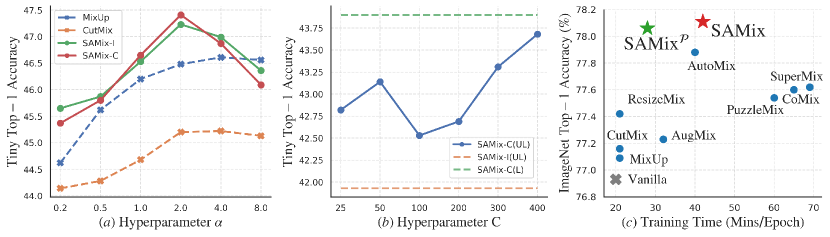
Figure 7: (a) Hyper-parameter $\alpha$ for mixup. (b) The cluster number $C$ for SAMix-C in CL tasks on Tiny. (c) Top-1 accuracy v.s. training time on IN-1k based on ResNet-50 with 100 epochs.

Table 9: Ablation of the learning objectives in the SSL tasks on STL-10 and Tiny-ImageNet.

method	STL-10	Tiny
BCE	85.25	41.28
infoNCE	85.36	41.85
infoNCE ($\eta=0.5$)	85.44	41.97
CE (PL)	85.56	42.36
CE (PL)+infoNCE	85.41	42.12
CE (PL, $\eta=0.5$)	85.60	42.53

Table 10: Ablation of proposed modules in Mixer and the $\eta$-balanced loss on Tiny.

module	SL	CL
Mixing attention	67.17	40.58
+Adaptive $\lambda$	67.95	41.82
+Non-linear content	68.46	42.45
+$\mathcal{L}_{mask}$	68.57	42.68
+$\lambda$ adjusting	68.61	43.14
+$\ell_{\eta}$ ($\eta=0.5$)	68.82	43.68

5 Related Work

Class-level Mixup for SL There are four types sample mixing policies for class-level mixup: linear mixup of input space [5, 19, 50, 51, 52] and latent space [53, 54], saliency-based [12, 6, 11], generation-based [13, 55], and learning mixup generation and classification end-to-end [16, 24]. More recently, mixup designed for ViTs optimizes mixing policies with self-attention maps [56, 57]. SAMix belongs to the fourth type and learns both class- and instance-level mixup relationships and its pre-trained SAMix^P eliminates high time-consuming problems of this type of method. Additionally, some researchers [58, 56, 59] improve class mixing policies upon linear mixup. See A.7 for details.

Instance-level Mixup for SSL A complementary method to learn better instance-level representation is to apply mixup in SSL scenarios [7]. However, most approaches are limited to using linear mixup variants, such as applying MixUp and CutMix in the input or latent space mixup [14, 41, 43, 44] for SSL without ground-truth labels. SAMix improves SSL tasks by learning mixup policies online.

6 Limitations and Conlusions

In this work, we first study and decompose objectives for mixup generation as local-emphasized and global-constrained terms in order to learn adaptive mixup policy at both class- and instance-level. SAMix provides a unified mixup framework with both online and pre-trained pipelines to boost discriminative representation learning based on improved $\eta$-balanced loss and Mixer. Moreover, a more applicable pre-trained SAMix^P is provided. As a limitation, the Mixer only takes two samples as input and conflicts when the task-relevant information is overlapping. In future works, we suppose that k-mixup (k$\geq$2) or conflict-aware Mixer can be another promising avenue to improve mixup.

Appendix A Appendix

We first introduce dataset information in A.1 and provide implementation details for supervised (SL) and self-supervised learning (SSL) tasks in A.2, A.3, and A.4. Then, we provide settings and results of analysis experiments for Sec. 3 in A.5. Moreover, we visualize mixed samples in A.6, and provide detailed related work in A.7.

A.1 Basic Settings

Reproduction details.

We use OpenMixup [60] implemented in PyTorch [36] as our code-base for both supervised image classification and contrastive learning (CL) tasks. Except results marked by ${\dagger}$ and $\ddagger$, we reproduce most experiment results of compared methods, including Mixup [5], CutMix [19], ManifoldMix [53], SaliencyMix [12], FMix [51], and ResizeMix [52].

Dataset information.

We briefly introduce image datasets used in Sec. 4: (1) CIFAR-100 [25] contains 50k training images and 10K test images of 100 classes. (2) ImageNet-1k (IN-1k) [61] contains 1.28 million training images and 50k validation images of 1000 classes. (3) Tiny-ImageNet (Tiny) [26] is a rescaled version of ImageNet-1k, which has 100k training images and 10k validation images of 200 classes. (4) STL-10 [28] benchmark is designed for semi- or unsupervised learning, which consists of 5k labeled training images for 10 classes 100K unlabelled training images, and a test set of 8k images. (5) CUB-200-2011 (CUB) [29] contains over 11.8k images from 200 wild bird species for fine-grained classification. (6) FGVC-Aircraft (Aircraft) [30] contains 10k images of 100 classes of aircraft. (7) iNaturalist2017 (iNat2017) [31] is a large-scale fine-grained classification benchmark consisting of 579.2k images for training and 96k images for validation from over 5k different wild species. (8) PASCAL VOC [45] is a classical objection detection and segmentation dataset containing 16.5k images for 20 classes. (9) COCO [46] is an objection detection and segmentation benchmark containing 118k scenic images with many objects for 80 classes.

A.2 Implementation of SAMix

Online training pipeline.

We provide the detailed implementation of SAMix in SL tasks. As shown in Figure 5 (left), we adopt the momentum pipeline [20, 16] to optimize $\mathcal{L}_{\theta,\omega}$ for mixup classification and $\mathcal{L}_{\phi}$ for mixup generation in Eq. 5 in an end-to-end manner:

$$\theta_{q}^{t},\omega_{q}^{t} \leftarrow\mathop{{\rm argmin}}\limits_{\theta,\omega}\mathcal{L}_{\theta_{q}^{t-1},\omega_{q}^{t-1}},$$ (12)

$$\phi^{t} \leftarrow\mathop{{\rm argmin}}\limits_{\phi}\mathcal{L}_{\theta_{k}^{t},\omega_{k}^{t}}+\mathcal{L}_{\phi^{t-1}},$$ (13)

where $t$ is the iteration step, $\theta_{q},\omega_{q}$ and $\theta_{k},\omega_{k}$ denote the parameters of online and momentum networks, respectively. The parameters in the momentum networks are an exponential moving average of the online networks with a momentum decay coefficient $m$, taking $\theta_{k}$ as an example,

$$\theta_{k}^{t}\leftarrow m\theta_{k}^{t-1}+(1-m)\theta_{q}^{t}.$$ (14)

The training process of SAMix is summarized as four steps: (1) using the momentum encoder to generate the feature maps $Z^{l}$ for Mixer $\mathcal{M}_{\phi}$; (2) generating $X_{mix}^{q}$ and $X_{mix}^{k}$ by Mixer for the online networks and Mixer; (3) training the online networks by Eq. 12 and the Mixer by Eq. 13 separately; (4) updating the momentum networks by Eq. 14.

Prior knowledge of mixup.

As we discussed in Sec. 3.2, we introduce some prior knowledge to the Mixer from two aspects: (a) To adjust the mean of $s_{i}$ correlated with $\lambda$, we introduce a mask loss that aligns the mean of $s_{i}$ to $\lambda$, $\ell_{\mu}=\beta\max(|\lambda-\mu_{i}|-\epsilon,0)$, where $\mu_{i}=\frac{1}{HW}\sum_{h,w}s_{i,h,w}$ is the mean and $\epsilon=0.1$ as a margin. Meanwhile, we propose a test time $\lambda$ adjusting method. Assuming $\mu_{i}<\lambda$, we adjust each coordinate on $s_{i}$ as $\hat{s}_{i}=\frac{\mu_{i}}{\lambda}s_{i}$, and $\hat{s}_{j}=1-\hat{s}_{i}$. (b) To balance the smoothness of local image patches and the discrimination (e.g., variance) of $x_{m}$, we adopt a bilinear upsampling as $U(\cdot)$ for smoother masks and propose a variance loss to encourage the sparsity of learned masks, $\ell_{\sigma}=\frac{1}{WH}\sum_{w,h}(\mu_{i}-s_{w,h})^{2}$. We summarize the mask loss as, $\mathcal{L}_{\phi}^{mask}=\beta(\ell_{\mu}+\ell_{\sigma})$, where $\beta$ is a balancing weight. $\beta$ is initialized to $0.1$ and linearly decreases to 0 during training.

A.3 Supervised Image Classification

Hyper-parameter settings.

As for hyper-parameters of SAMix, we follow the basic setting in AutoMix for both SL and SSL tasks: SAMix adopts $\alpha=2$, the feature layer $l=3$, the bilinear upsampling, and the weight $\beta=0.1$ which linearly decays to $0$. We use $\eta=0.5$ for small-scale datasets (CIFAR-100, Tiny, CUB and Aircraft) and $\eta=0.1$ for large-scale datasets (IN-1k and iNat2017). As for other methods, PuzzleMix [6], Co-Mixup [11], and AugMix [50] are reproduced by their official implementations with $\alpha=1,2,1$ for all datasets. As for mixup methods reproduced by us, we provide dataset-specific hyper-parameter settings as follows. For CIFAR-100, Mixup and ResizeMix use $\alpha=1$, and CutMix, FMix and SaliencyMix use $\alpha=0.2$, and ManifoldMix uses $\alpha=2$. For Tiny, IN-1k, and iNat2017 datasets, ManifoldMix uses $\alpha=0.2$, and the rest methods adopt $\alpha=1$ for median and large backbones (e.g., ResNet-50). Specially, all these methods use $\alpha=0.2$ (only) for ResNet-18. For small-scale fine-grained datasets (CUB-200 and Aircraft), SaliencyMix and FMix use $\alpha=0.2$, and ManifoldMix uses $\alpha=0.5$, while the rest use $\alpha=1$.

A.4 Contrastive Learning

Implementation of SAMix-C and SAMix-I.

As for SSL tasks, we adopt the cross-view objective, $\ell^{NCE}(z_{i}^{\tau_{q}},z_{i}^{\tau_{k}})+\ell^{NCE}(z_{m})$, where $z_{i}=z_{i}^{\tau_{k}}$ and $z_{j}=z_{j}^{\tau_{k}}$, for instance-level mixup classification in all methods (except for ${\dagger}$ and $\ddagger$ marked methods). We provide two variants, SAMix-C and SAMix-I, which use different learning objectives of mixup classification. The basic network structures (an encoder $f_{\theta}$ and a projector $g_{\omega}$) are adopted as MoCo.V2 [62]. Similar to SAMix in SL tasks, SAMix-C employs a parametric cluster classification head $g_{\psi}^{C}$ for online clustering [63, 21] to provide pseudo labels (PL) to calculate $\mathcal{L}_{\phi}^{cls}$. It takes feature vectors from the momentum encoder as the input (optimized by Eq. 13) and has no impact on the mixup classification objective for the online networks. Meanwhile, SAMix-I employs the instance-level classification loss for both $\mathcal{L}_{\theta,\omega}$ and $\mathcal{L}_{\phi}^{cls}$. Moreover, we use the proposed $\eta$-balanced mixup loss $\mathcal{L}_{\phi}^{cls}$ for both SAMix-C and SAMix-I with $\eta=0.5$ and the objective $\mathcal{L}_{\phi}$ for Mixer.

Hyper-parameter settings.

As for Table 5 and Table 6, all compared CL methods use MoCo.V2 pre-training settings except for SwAV [42], which adopts ResNet-50 [64] as the encoder $f_{\theta}$ with two-layer MLP projector $g_{\omega}$ and is optimized by SGD optimizer and Cosine scheduler with the initial learning rate of $0.03$ and the batch size of $256$. The length of the momentum dictionary is 65536 for IN-1k and 16384 for STL-10 and Tiny datasets. The data augmentation strategy is based on IN-1k in MoCo.v2 as follows: Geometric augmentation is RandomResizedCrop with the scale in $[0.2,1.0]$ and RandomHorizontalFlip. Color augmentation is ColorJitter with {brightness, contrast, saturation, hue} strength of $\{0.4,0.4,0.4,0.1\}$ with a probability of $0.8$, and RandomGrayscale with a probability of $0.2$. Blurring augmentation uses a square Gaussian kernel of size $23\times 23$ with a std uniformly sampled in $[0.1,2.0]$. We use 224$\times$224 resolutions for IN-1k and 96$\times$96 resolutions for STL-10 and Tiny datasets. As for Table 7 and Table 8, we follow the original setups of these CL baselines (SimCLR [4], MoCo.V1 [65], MoCo.V2 [62], BYOL [20], SwAV [42], SimSiam [66], and MoCo.V3 [67]) using OpenMixup [60] implementations. Notice that MoCo.V3 is specially designed for vision Transformers [8] while other CL baselines are originally proposed with CNN architecture. Meanwhile, we employ the contrastive learning objectives with mixing augmentations for BYOL and SimSiam proposed in BSIM [41] because these CL baselines adopt the MSE loss between positive sample pairs instead of the infoNCE loss (Eq. 2).

CL methods with Mixup augmentations.

In Sec. 4.2, we compare the proposed SAMix variants with general Mixup approaches proposed in SL and well-designed CL methods with Mixups. As for the general Mixup variants implemented with CL baselines, Mixup [5], ManifoldMix [53], CutMix [19], SaliencyMix [12], FMix [51], ResizeMix [52], PuzzleMix [6], and out proposed SAMix only use the single Mixup augmentation. As for the CL methods applying Mixup augmentations, DACL [43] employs the vanilla Mixup, MoCHi [14], i-Mix [7], UnMix [15], WBSIM [41] use two types of Mixup strategies in the input image and the latent space of the encoder, SDMP [44] randomly applies three types of input space Mixups (Mixup, CutMix, and ResizeMix). Therefore, SDMP can achieve competitive performances as SAMix variants in Table 7 and Table 8.

Evaluation protocols.

We evaluate the SSL representation with a linear classification protocol proposed in MoCo [17] and MoCo.V3 [67] for ResNet and ViT variants, which trains a linear classifier on top of the frozen representation on the training set. For ResNet variants, the linear classifier is trained 100 epochs by an SGD optimizer with the SGD momentum of $0.9$ and the weight decay of $0$. We set the initial learning rate of $30$ for IN-1k as MoCo, and $0.1$ for STL-10 and Tiny with a batch size of 256. The learning rate decays by $0.1$ at epochs 60 and 80. For ViT-S, the linear classifier is trained 90 epochs by the SGD optimizer with a batch size of 1024 and a basic learning rate of 12. Moreover, we adopt object detection task to evaluate transfer learning abilities following MoCo, which uses the $4$-th layer feature maps of ResNet (ResNet-C4) to fine-tune Faster R-CNN [48] with 24k iterations on the trainval07+12 set and Mask R-CNN [49] with 2$\times$ training schedule (24-epoch) on the train2017 set.

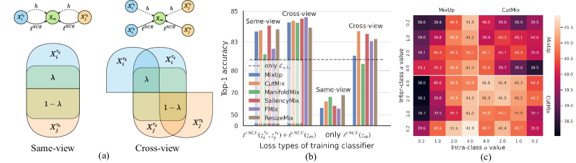
Figure 8: (a) Graphical models and information diagrams of same-view and cross-view training pipeline for instance-level mixup. Taking the cross-view as an example, $x_{m}=h(x_{i}^{\tau_{2}},x_{j}^{\tau_{2}},\lambda)$, the $\lambda$ region denotes the corresponding information partition for $\lambda I(z_{m}^{\tau_{q}},z_{i}^{\tau_{k}})$ and the $1-\lambda$ region for $(1-\lambda)I(z_{m}^{\tau_{q}},z_{j}^{\tau_{k}})$. (b) Linear evaluation (top-1 accuracy on STL-10) of whether to use the cross-view pipeline and to combine the original infoNCE loss with the mixup infoNCE loss. (c) A heat map of linear evaluation (top-1 accuracy on Tiny) represents the effects of using MixUp and CutMix as the inter-class (y-axis) and intra-class mixup (x-axis) using various $\alpha$.

A.5 Empirical Experiments

A.5.1 Cross-view Training Pipeline for Instance-level Mixup

We first analyze the learning objective of instance-level mixup classification for contrastive learning (CL) as discussed in Sec. 2.2. As shown in Figure 8 (a), there are two possible objectives for instance-level mixup defined in Eq. 4: the same-view, $\mathop{\max}\limits_{\theta,\omega}\lambda I(z_{m}^{\tau_{q}},z_{i}^{\tau_{q}})+(1-\lambda)I(z_{m}^{\tau_{q}},z_{j}^{\tau_{q}})$, and cross-view objective, $\mathop{\max}\limits_{\theta,\omega}\lambda I(z_{m}^{\tau_{q}},z_{i}^{\tau_{k}})+(1-\lambda)I(z_{m}^{\tau_{q}},z_{j}^{\tau_{k}})$. We hypothesize that the cross-view objective yields better CL performance than the same-view because the mutual information between two augmented views should be reduced while keeping task-relevant information [68, 69]. To verify this hypothesis, we design an experiment of various mixup methods with $\alpha=1$ on STL-10 with ResNet-18. As shown in Figure 8 (b), we compare using the same-view or cross-view pipelines combined with using $\ell^{NCE}(z_{i}^{\tau_{q}},z_{i}^{\tau_{k}})+\ell^{NCE}(z_{m})$ or only using $\ell^{NCE}(z_{m})$. We can conclude: (i) Degenerated solutions occur when using the same-view pipeline while using the cross-view pipeline outperforms the CL baseline. It is mainly caused by degenerated mixed samples which contain parts of the same view of two source images. Therefore, we propose the cross-view pipeline for the instance-level mixup, where $z_{i}$ and $z_{j}$ in Eq. 4 are representations of $x_{i}^{\tau_{k}}$ and $x_{j}^{\tau_{k}}$. (ii) Combining both the original and mixup infoNCE loss, $\ell^{NCE}(z_{i}^{\tau_{q}},z_{i}^{\tau_{k}})+\ell^{NCE}(z_{m})$, surpasses only using one of them, which indicates that mixup enables $f_{\theta}$ to learn the relationship between local neighborhood systems.

A.5.2 Analysis of Instance-level Mixup

As we discussed in Sec. A.5.1, we propose the cross-view training pipeline for instance-level mixup classification. We then discuss inter- and intra-class proprieties of instance-level mixup. As shown in Figure 8 (c), we adopt inter-cluster and intra-cluster mixup from {Mixup, CutMix} with $\alpha\in\{0.2,1,2,4\}$ to verify that instance-level mixup should treat inter- and intra-class mixup differently. Empirically, mixed samples provided by Mixup preserve global information of both source samples (smoother), while samples generated by CutMix preserve local patches (more discriminative). And we introduce pseudo labels (PL) to indicate different clusters by clustering method ODC [21] with the class (cluster) number $C$. Based on experiment results, we can conclude that inter-class mixup requires discriminative mixed samples with strong intensity while the intra-class needs smooth samples with low intensity. Moreover, we provide two cluster-based instance-level mixup methods in Table 5 and 6 (denoting by $*$): (a) Inter-Intra^∗. We use CutMix with $\alpha\geq 2$ as inter-cluster mixup and Mixup with $\alpha=0.2$ as an intra-cluster mixup. (b) PuzzleMix^∗. We introduce saliency-based mixup methods to SSL tasks by introducing PL and a parametric cluster classifier $g_{\psi}^{C}$ after the encoder. This classifier $g_{\psi}^{C}$ and encoder $f_{\theta}$ are optimized online like AutoMix and SAMix mentioned in A.2. Based on Grad-CAM [10] calculated from the classifier, PuzzleMix can be adopted on SSL tasks.

A.5.3 Analysis of Mixup Generation Objectives

In Sec. 3.1, we design experiments to analyze various losses for mixup generation in Figure 2 (left) and the proposed $\eta$-balanced loss in Figure 2 (right) for both SL and SSL tasks with ResNet-18 on STL-10 and Tiny. Basically, we assume both STL-10 and Tiny datasets have 200 classes on their 100k images. Since STL-10 does not provide ground truth labels (L) for 100k unlabeled data, we introduce PL generated by a supervised pertained classifier on Tiny as the "ground truth" for its 100k training set. Notice that L denotes ground truth labels and PL denotes pseudo labels generated by ODC [21] with $C=200$.

As for the SL task, we use the labeled training set for mixup classification (100k on Tiny v.s. 5k on STL-10). Notice that SL results are worse than using SSL settings on STL-10, since the SL task only trains a randomly initialized classifier on 5k labeled data. Because the infoNCE and BCE loss require cross-view augmentation (or they will produce trivial solutions), we adopt MoCo.V2 augmentation settings for these two losses when performing the SL task. Compared to CE (L), we corrupt the global term in CE as CE (PL) or directly remove them as pBCE (L) to show that pBCE is vital to optimizing mixed samples. Similarly, we show that the global term is used as the global constraint by comparing BCE (UL) with infoNCE (UL), infoNCE (PL), and infoNCE (L).

As for the SSL task, we verify the conclusions drawn from the SL task and conclude that (a) the local term optimizes mixup generation directly, corresponding to the smoothness property, and (b) the global term serves as the global constraint corresponding to the discriminative property. Moreover, we verified that using the $\eta$-balanced loss as $\mathcal{L}_{\phi}^{cls}$ yields the best performance on SL and SSL tasks. Notice that we use $\eta=0.5$ on small-scale datasets and $\eta=0.1$ on large-scale datasets for SL tasks, and use $\eta=0.5$ for all SSL tasks.

Table 11: Transferring to object detection with Faster R-CNN on VOC and Mask R-CNN on COCO.

		Faster R-CNN			Mask R-CNN
CL Method	Methods	AP	AP50	AP75	APb	AP${}_{50}^{b}$	AP${}_{75}^{b}$
MoCo.V2	-	56.9	82.2	63.4	40.6	60.1	44.0
MoCo.V2	Mixup	57.4	82.5	64.0	41.0	60.8	44.3
MoCo.V2	CutMix	57.3	82.7	64.1	41.1	60.8	44.4
MoCo.V2	Inter-Intra⋆	57.5	82.8	64.2	41.2	60.9	44.4
MoCHi†	$input$+$latent$	57.1	82.7	64.1	41.0	60.8	44.5
i-Mix†	$input$+$latent$	57.5	82.7	64.2	-	-	-
UnMix‡	$input$+$latent$	57.7	83.0	64.3	41.2	60.9	44.7
WBSIM‡	$input$	57.4	82.8	64.2	40.7	60.8	44.2
MoCo.V2	SAMix-I	57.5	83.1	64.2	41.2	61.0	44.5
MoCo.V2	SAMix-IP	57.8	83.2	64.3	41.3	61.1	44.6
MoCo.V2	SAMix-C	57.7	83.1	64.4	41.3	61.1	44.7

A.5.4 Analysis of Mutual Information for Mixup

Since mutual information (MI) is usually adopted to analyze contrastive-based augmentations [70, 68], we estimate MI between $x_{m}$ of various methods and $x_{i}$ by MINE [71] with 100k images in 64$\times$64 resolutions on Tiny-ImageNet. We sample $\lambda=$ from 0 to 1 with the step of $0.125$ and plot results in Figure 7 (d). Here we see that SAMix-C and SAMix-I with more MI when $\lambda\approx 0.5$ perform better.

A.5.5 Results of Downstream tasks

In Sec. 4.2, we evaluate transferable abilities of the learned representation of self-supervised methods to object detection task on PASCAL VOC [45] and COCO [46]. In Table 11, the online SAMix-C and the pre-trained SAMix-I^P achieve the best detection performances among the compared methods and significantly improves the baseline MoCo.V2 (e.g., SAMix-C gains 0.9% AP and +0.7% AP^b over MoCo.V2). Notice that MoCHi, i-Mix, and UnMix introduce mixup augmentations in both the input and latent spaces, while our proposed SAMix only generates mixed samples in the input space.

A.6 Visualization of SAMix

A.6.1 Mixing Attention and Content in Mixer

In Sec. 3.2, we discuss the trivial solutions of Mixer, which are usually occurred in SSL tasks. Given the sample pair $(x_{i},x_{j})$ and $\lambda=0.5$, we visualize the content $C_{i}$ and $P_{i,j}$ to compare the trivial and non-trivial results in the SSL task on STL-10, as shown in Figure 3. As we can see, both $C_{i}$ and $P_{i,j}$ from the trivial solution has extremely large or small scale values while $C_{i}$ generated by $C_{NCL}$ containing more balanced values. Since the attention weight $P_{i,j}$ is normalized by softmax, we hypothesize that $C_{i}$ more likely causes trivial solutions. To verify our hypothesis, we freeze $W_{P}$ in the original MB and compare the original linear content projection $W_{z}$ with the non-linear content modeling. The results confirm that the non-linear module can prevent large-scale values on $C_{i}$ and eliminate the trivial solutions.

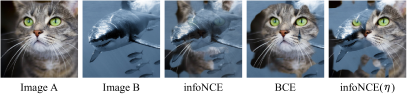
Figure 9: Visualization of loss effect. Both infoNCE and BCE loss have different emphases: infoNCE shows a similar effect of supervised fine-grained classification, focusing on fragmented and essential features, while BCE focuses on object completeness.

A.6.2 Effects of Mixup Generation Loss

In addition to Sec.3.3, we further provide visualization of mixed samples using the infoNCE (Eq. 4), BCE (Eq. 7), and $\eta$-balanced infoNCE loss (Eq. 8) for Mixer. As shown in Figure 9, we find that mixed samples using infoNCE mixup loss prefer instance-specific and fine-grained features. On the contrary, mixed samples of the BCE loss seem only to consider discrimination between two corresponding neighborhood systems. It is more inclined to maintain the continuity of the whole object relative to infoNCE. Thus, combining both the characteristics, the $\eta$-balanced infoNCE loss yields mixed samples that retain both instance-specific features and global discrimination.

A.6.3 Visualization of Mixed Samples in SAMix

SAMix in various scenarios.

In addition to Sec. 3.3, we visualize the mixed samples of SAMix in various scenarios to show the relationship between mixed samples and class (cluster) information. Since IN-1k contains some samples in CUB and Aircraft, we choose the overlapped samples to visualize SAMix trained for the fine-grained SL task (CUB and Aircraft) and SSL tasks (SAMix-I and SAMix-C). As shown in Figure 10, mixed samples reflect the granularity of class information adopted in mixup training. Specifically, we find that mixed samples using infoNCE mixup loss (Eq.4) is more closely to the fine-grained SL because they both have many fine-grained centroids.

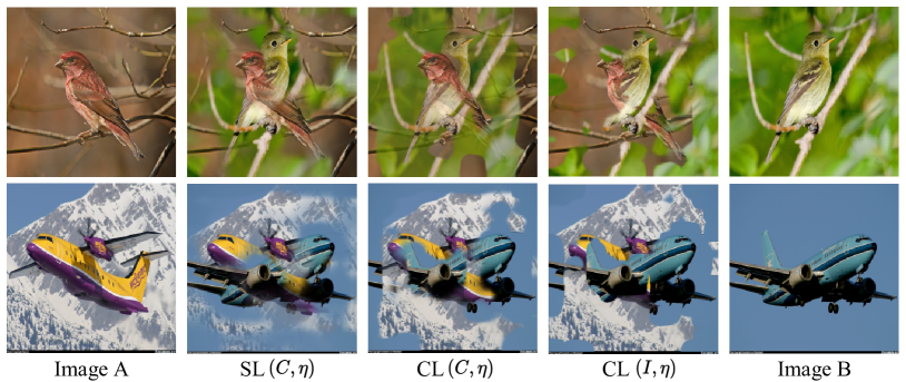
Figure 10: Visualization of SAMix in various scenarios on CUB and Aircraft. Given images A and B, the middle three mixed samples are generated by SAMix with $\lambda=0.5$ trained in the fine-grained SL task and the SSL tasks (SAMix-C and SAMix-I).

Comparison with PuzzleMix in SL tasks.

To highlight the accurate mixup relationship modeling in SAMix compared to PuzzleMix (standing for saliency-based methods), we visualize the results of mixed samples from these two methods in the supervised case in Figure 11. There is three main difference: (a) bilinear upsampling strategy in SAMix makes the mixed samples more smooth in local patches. (b) adaptive $\lambda$ encoding and mixing attention enhances the correspondence between mixed samples and $\lambda$ value. (c) $\eta$-balanced mixup loss enables SAMix to balance global discriminative and fine-grained features.

Comparison of SAMix-I and SAMix-C in SSL tasks.

As shown in Figure 12, we provide more mixed samples of SAMix-I and SAMix-C in the SSL tasks to show that introducing class information by PL can help Mixer generate mixed samples that retain both the fine-grained features (instance discrimination) and whole targets.

A.7 Detailed related work

Contrastive Learning.

CL amplifies the potential of SSL by achieving significant improvements on classification [4, 17, 42], which maximizes similarities of positive pairs while minimizing similarities of negative pairs. To provide a global view of CL, MoCo [17] proposes a memory-based framework with a large number of negative samples and model differentiation using the exponential moving average. SimCLR [4] demonstrates a simple memory-free approach with large batch size and strong data augmentations that is also competitive in performance to memory-based methods. BYOL [20] and its variants [66, 67] do not require negative pairs or a large batch size for the proposed pretext task, which tries to estimate latent representations from the same instance. Besides pairwise contrasting, SwAV [42] performs online clustering while enforcing consistency between multi-views of the same image. Barlow Twins [72] avoids the representation collapsing by learning the cross-correlation matrix of distorted views of the same sample. Moreover, MoCo.V3 [67] and DINO [73] are proposed to tackle unstable issues and degenerated performances of CL based on popular Vision Transformers [8].

Mixup.

MixUp [5], convex interpolations of any two samples and their unique one-hot labels were presented as the first mixing-based data augmentation approach for regularising the training of networks. ManifoldMix [53] and PatchUp [54] expand it to the hidden space. CutMix [19] suggests a mixing strategy based on the patch of the image, i.e., randomly replacing a local rectangular section in images. Based on CutMix, ResizeMix [52] inserts a whole image into a local rectangular area of another image after scaling down. FMix [51] converts the image to Fourier space (spectrum domain) to create binary masks. To generate more semantic virtual samples, offline optimization algorithms are introduced for the saliency regions. SaliencyMix [12] obtains the saliency using a universal saliency detector. With optimization transportation, PuzzleMix [6] and Co-Mixup [11] present more precise methods for finding appropriate mixup masks based on saliency statistics. SuperMix [24] combines mixup with knowledge distillation, which learns a pixel-wise sample mixing policy via a teacher-student framework. More recently, TransMix [56] and TokenMix [57] are proposed specially designed Mixup augmentations for Vision Transformers [8]. Differing from previous methods, AutoMix [16] can learn the mixup generation by a sub-network end-to-end, which generates mixed samples via feature maps and the mixing ratio. Orthogonal to the sample mixing strategies, some researchers [58, 56, 59] improve the label mixing policies upon linear mixup.

Mixup for contrastive learning.

A complementary method for better instance-level representation learning is to use mixup on CL [14, 15]. When used in collaboration with CE loss, Mixup and its several variants provide highly efficient data augmentation for SL by establishing a relationship between samples. Most approaches are limited to linear mixup methods without a ground-truth label. For example, Un-mix [15] attempts to use MixUp in the input space for self-supervised learning, whereas the developers of MoChi [14] propose mixing the negative sample in the embedding space to increase the number of hard negatives but at the expense of classification accuracy. i-Mix [7], DACL [43], BSIM [41] and SDMP [44] demonstrated how to regularize contrastive learning by mixing instances in the input or latent spaces. We introduce an automatic mixup for SSL tasks, which adaptively learns the instance relationship based on inter- and intra-cluster properties online.

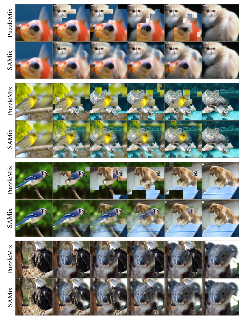
Figure 11: Visualization of PuzzleMix v.s. SAMix for SL tasks on IN-1k. In every four rows, the upper and lower two rows represent mixed samples generated by PuzzleMix and SAMix, respectively. $\lambda$ value changes from left ($\lambda=0$) to right ($\lambda=1$) by an equal step.

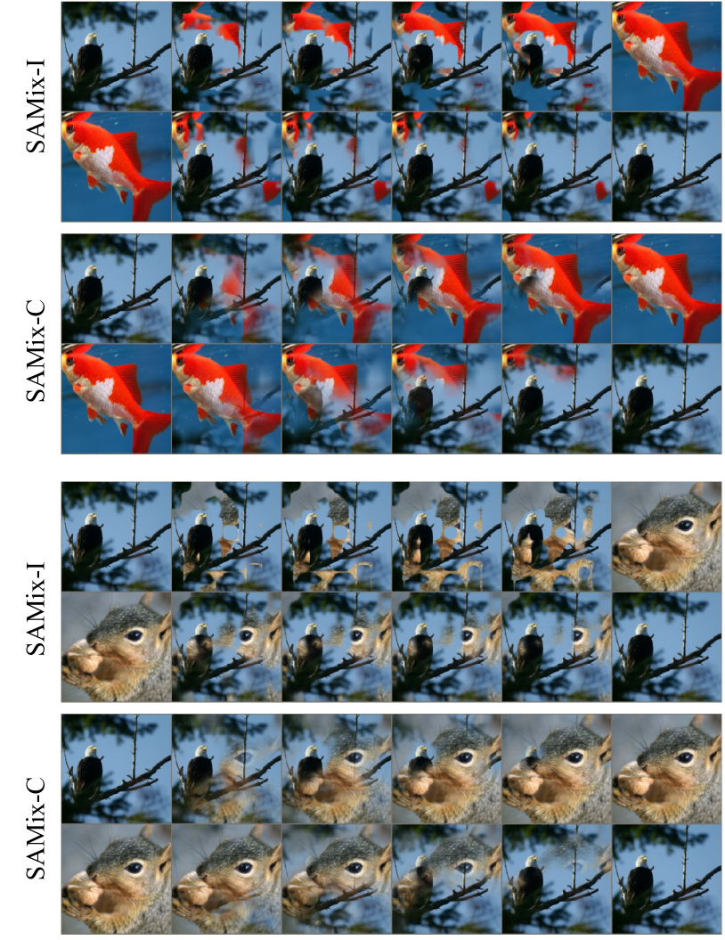
Figure 12: Visualization of SAMix-I v.s. SAMix-C for SSL tasks on IN-1k. In every four rows, the upper and lower two rows represent mixed samples generated by SAMix-I and SAMix-C, respectively. $\lambda$ value changes from left ($\lambda=0$) to right ($\lambda=1$) by an equal step.

References

- [1] Yoshua Bengio, Aaron Courville, and Pascal Vincent. Representation learning: A review and new perspectives. IEEE transactions on pattern analysis and machine intelligence, 35(8):1798–1828, 2013.
- [2] Jacob Devlin, Ming-Wei Chang, Kenton Lee, and Kristina Toutanova. Bert: Pre-training of deep bidirectional transformers for language understanding. arXiv preprint arXiv:1810.04805, 2018.
- [3] Bruno Korbar, Du Tran, and Lorenzo Torresani. Cooperative learning of audio and video models from self-supervised synchronization. arXiv preprint arXiv:1807.00230, 2018.
- [4] Ting Chen, Simon Kornblith, Mohammad Norouzi, and Geoffrey Hinton. A simple framework for contrastive learning of visual representations. In Proceedings of the International Conference on Machine Learning (ICML), 2020.
- [5] Hongyi Zhang, Moustapha Cisse, Yann N Dauphin, and David Lopez-Paz. mixup: Beyond empirical risk minimization. In International Conference on Learning Representations (ICLR), 2018.
- [6] Jang-Hyun Kim, Wonho Choo, and Hyun Oh Song. Puzzle mix: Exploiting saliency and local statistics for optimal mixup. In International Conference on Machine Learning (ICML), pages 5275–5285. PMLR, 2020.
- [7] Kibok Lee, Yian Zhu, Kihyuk Sohn, Chun-Liang Li, Jinwoo Shin, and Honglak Lee. I-mix: A domain-agnostic strategy for contrastive representation learning. In International Conference on Learning Representations (ICLR), 2021.
- [8] Alexey Dosovitskiy, Lucas Beyer, Alexander Kolesnikov, Dirk Weissenborn, Xiaohua Zhai, Thomas Unterthiner, Mostafa Dehghani, Matthias Minderer, Georg Heigold, Sylvain Gelly, Jakob Uszkoreit, and Neil Houlsby. An image is worth 16x16 words: Transformers for image recognition at scale. In International Conference on Learning Representations (ICLR), 2021.
- [9] Hugo Touvron, M. Cord, M. Douze, F. Massa, Alexandre Sablayrolles, and H. Jégou. Training data-efficient image transformers & distillation through attention. In Proceedings of the International Conference on Machine Learning (ICML), 2021.
- [10] Ramprasaath R. Selvaraju, Michael Cogswell, Abhishek Das, Ramakrishna Vedantam, Devi Parikh, and Dhruv Batra. Grad-cam: Visual explanations from deep networks via gradient-based localization. arXiv preprint arXiv:1610.02391, 2019.
- [11] Jang-Hyun Kim, Wonho Choo, Hosan Jeong, and Hyun Oh Song. Co-mixup: Saliency guided joint mixup with supermodular diversity. In International Conference on Learning Representations (ICLR), 2021.
- [12] AFM Uddin, Mst Monira, Wheemyung Shin, TaeChoong Chung, Sung-Ho Bae, et al. Saliencymix: A saliency guided data augmentation strategy for better regularization. In International Conference on Learning Representations (ICLR), 2021.
- [13] Jianchao Zhu, Liangliang Shi, Junchi Yan, and Hongyuan Zha. Automix: Mixup networks for sample interpolation via cooperative barycenter learning. In European Conference on Computer Vision (ECCV). Springer, 2020.
- [14] Yannis Kalantidis, Mert Bulent Sariyildiz, Noe Pion, Philippe Weinzaepfel, and Diane Larlus. Hard negative mixing for contrastive learning. In Advances in Neural Information Processing Systems (NeurIPS), 2020.
- [15] Zhiqiang Shen, Zechun Liu, Zhuang Liu, Marios Savvides, Trevor Darrell, and Eric Xing. Un-mix: Rethinking image mixtures for unsupervised visual representation learning. In Proceedings of the AAAI Conference on Artificial Intelligence (AAAI), 2021.
- [16] Zicheng Liu, Siyuan Li, Di Wu, Zhiyuan Chen, Lirong Wu, Jianzhu Guo, and Stan Z Li. Automix: Unveiling the power of mixup. In Proceedings of the European Conference on Computer Vision (ECCV). Springer, 2022.
- [17] Kaiming He, Haoqi Fan, Yuxin Wu, Saining Xie, and Ross Girshick. Momentum contrast for unsupervised visual representation learning. In Proceedings of the IEEE/CVF Conference on Computer Vision and Pattern Recognition (CVPR), pages 9729–9738, 2020.
- [18] Aaron van den Oord, Yazhe Li, and Oriol Vinyals. Representation learning with contrastive predictive coding. arXiv preprint arXiv:1807.03748, 2019.
- [19] Sangdoo Yun, Dongyoon Han, Seong Joon Oh, Sanghyuk Chun, Junsuk Choe, and Youngjoon Yoo. Cutmix: Regularization strategy to train strong classifiers with localizable features. In Proceedings of the IEEE/CVF International Conference on Computer Vision (ICCV), pages 6023–6032, 2019.
- [20] Jean-Bastien Grill, Florian Strub, Florent Altché, Corentin Tallec, Pierre H Richemond, Elena Buchatskaya, Carl Doersch, Bernardo Avila Pires, Zhaohan Daniel Guo, Mohammad Gheshlaghi Azar, et al. Bootstrap your own latent: A new approach to self-supervised learning. In Advances in Neural Information Processing Systems (NeurIPS), 2020.
- [21] Xiaohang Zhan, Jiahao Xie, Ziwei Liu, Yew Soon Ong, and Chen Change Loy. Online deep clustering for unsupervised representation learning. In Proceedings of the Conference on Computer Vision and Pattern Recognition (CVPR), 2020.
- [22] Prannay Khosla, Piotr Teterwak, Chen Wang, Aaron Sarna, Yonglong Tian, Phillip Isola, Aaron Maschinot, Ce Liu, and Dilip Krishnan. Supervised contrastive learning. In Advances in Neural Information Processing Systems (NeurIPS), 2020.
- [23] Joshua David Robinson, Ching-Yao Chuang, Suvrit Sra, and Stefanie Jegelka. Contrastive learning with hard negative samples. In International Conference on Learning Representations, 2021.
- [24] Ali Dabouei, Sobhan Soleymani, Fariborz Taherkhani, and Nasser M Nasrabadi. Supermix: Supervising the mixing data augmentation. In Proceedings of the IEEE/CVF Conference on Computer Vision and Pattern Recognition (CVPR), pages 13794–13803, 2021.
- [25] Alex Krizhevsky, Geoffrey Hinton, et al. Learning multiple layers of features from tiny images. 2009.
- [26] Patryk Chrabaszcz, Ilya Loshchilov, and Frank Hutter. A downsampled variant of imagenet as an alternative to the cifar datasets. arXiv preprint arXiv:1707.08819, 2017.
- [27] Olga Russakovsky, Jia Deng, Hao Su, Jonathan Krause, Sanjeev Satheesh, Sean Ma, Zhiheng Huang, Andrej Karpathy, Aditya Khosla, Michael Bernstein, et al. Imagenet large scale visual recognition challenge. International journal of computer vision (IJCV), pages 211–252, 2015.
- [28] Adam Coates, Andrew Ng, and Honglak Lee. An analysis of single-layer networks in unsupervised feature learning. In Proceedings of the fourteenth international conference on artificial intelligence and statistics, pages 215–223. JMLR Workshop and Conference Proceedings, 2011.
- [29] Catherine Wah, Steve Branson, Peter Welinder, Pietro Perona, and Serge Belongie. The caltech-ucsd birds-200-2011 dataset. California Institute of Technology, 2011.
- [30] Subhransu Maji, Esa Rahtu, Juho Kannala, Matthew Blaschko, and Andrea Vedaldi. Fine-grained visual classification of aircraft. arXiv preprint arXiv:1306.5151, 2013.
- [31] Grant Van Horn, Oisin Mac Aodha, Yang Song, Yin Cui, Chen Sun, Alex Shepard, Hartwig Adam, Pietro Perona, and Serge Belongie. The inaturalist species classification and detection dataset. In Proceedings of the Conference on Computer Vision and Pattern Recognition (CVPR), 2018.
- [32] Bolei Zhou, Agata Lapedriza, Jianxiong Xiao, Antonio Torralba, and Aude Oliva. Learning deep features for scene recognition using places database. In Advances in Neural Information Processing Systems (NeurIPS), pages 487–495, 2014.
- [33] Sergey Zagoruyko and Nikos Komodakis. Wide residual networks. In Proceedings of the British Machine Vision Conference (BMVC), 2016.
- [34] Saining Xie, Ross Girshick, Piotr Dollár, Zhuowen Tu, and Kaiming He. Aggregated residual transformations for deep neural networks. In Proceedings of the IEEE conference on computer vision and pattern recognition (CVPR), pages 1492–1500, 2017.
- [35] Ze Liu, Yutong Lin, Yue Cao, Han Hu, Yixuan Wei, Zheng Zhang, Stephen Lin, and Baining Guo. Swin transformer: Hierarchical vision transformer using shifted windows. In IEEE/CVF International Conference on Computer Vision (ICCV), 2021.
- [36] Adam Paszke, Sam Gross, Francisco Massa, Adam Lerer, James Bradbury, Gregory Chanan, Trevor Killeen, Zeming Lin, Natalia Gimelshein, Luca Antiga, Alban Desmaison, Andreas Köpf, Edward Yang, Zach DeVito, Martin Raison, Alykhan Tejani, Sasank Chilamkurthy, Benoit Steiner, Lu Fang, Junjie Bai, and Soumith Chintala. Pytorch: An imperative style, high-performance deep learning library. In Advances in Neural Information Processing Systems (NeurIPS), 2019.
- [37] Ilya Loshchilov and Frank Hutter. Sgdr: Stochastic gradient descent with warm restarts. arXiv preprint arXiv:1608.03983, 2016.
- [38] Yang You, Jing Li, Sashank Reddi, Jonathan Hseu, Sanjiv Kumar, Srinadh Bhojanapalli, Xiaodan Song, James Demmel, Kurt Keutzer, and Cho-Jui Hsieh. Large batch optimization for deep learning: Training BERT in 76 minutes. In International Conference on Learning Representations (ICLR), 2020.
- [39] Ross Wightman, Hugo Touvron, and Hervé Jégou. Resnet strikes back: An improved training procedure in timm. arXiv preprint arXiv:2110.00476, 2021.
- [40] Ilya Loshchilov and Frank Hutter. Decoupled weight decay regularization. In International Conference on Learning Representations (ICLR), 2019.
- [41] Xiangxiang Chu, Xiaohang Zhan, and Xiaolin Wei. A unified mixture-view framework for unsupervised representation learning. In Proceedings of the British Machine Vision Conference (BMVC), 2022.
- [42] Mathilde Caron, Ishan Misra, Julien Mairal, Priya Goyal, Piotr Bojanowski, and Armand Joulin. Unsupervised learning of visual features by contrasting cluster assignments. In Advances in Neural Information Processing Systems (NeurIPS), 2020.
- [43] Vikas Verma, Minh-Thang Luong, Kenji Kawaguchi, Hieu Pham, and Quoc V. Le. Towards domain-agnostic contrastive learning. In International Conference on Machine Learning (ICML), 2021.
- [44] Sucheng Ren, Huiyu Wang, Zhengqi Gao, Shengfeng He, Alan Loddon Yuille, Yuyin Zhou, and Cihang Xie. A simple data mixing prior for improving self-supervised learning. In Proceedings of the Conference on Computer Vision and Pattern Recognition (CVPR), pages 14575–14584, 2022.
- [45] Mark Everingham, Luc Van Gool, Christopher KI Williams, John Winn, and Andrew Zisserman. The pascal visual object classes (voc) challenge. International journal of computer vision (IJCV), 88(2):303–338, 2010.
- [46] Tsung-Yi Lin, Michael Maire, Serge Belongie, James Hays, Pietro Perona, Deva Ramanan, Piotr Dollár, and C Lawrence Zitnick. Microsoft coco: Common objects in context. In Proceedings of the European Conference on Computer Vision (ECCV), 2014.
- [47] Yuxin Wu, Alexander Kirillov, Francisco Massa, Wan-Yen Lo, and Ross Girshick. Detectron2. https://github.com/facebookresearch/detectron2, 2019.
- [48] Shaoqing Ren, Kaiming He, Ross Girshick, and Jian Sun. Faster r-cnn: Towards real-time object detection with region proposal networks. arXiv preprint arXiv:1506.01497, 2015.
- [49] Kaiming He, Georgia Gkioxari, Piotr Dollár, and Ross Girshick. Mask r-cnn. In Proceedings of the International Conference on Computer Vision (ICCV), 2017.
- [50] Dan Hendrycks, Norman Mu, Ekin D Cubuk, Barret Zoph, Justin Gilmer, and Balaji Lakshminarayanan. Augmix: A simple data processing method to improve robustness and uncertainty. In International Conference on Learning Representations (ICLR), 2020.
- [51] Ethan Harris, Antonia Marcu, Matthew Painter, Mahesan Niranjan, and Adam Prügel-Bennett Jonathon Hare. Fmix: Enhancing mixed sample data augmentation. arXiv preprint arXiv:2002.12047, 2(3):4, 2020.
- [52] Jie Qin, Jiemin Fang, Qian Zhang, Wenyu Liu, Xingang Wang, and Xinggang Wang. Resizemix: Mixing data with preserved object information and true labels. arXiv preprint arXiv:2012.11101, 2020.
- [53] Vikas Verma, Alex Lamb, Christopher Beckham, Amir Najafi, Ioannis Mitliagkas, David Lopez-Paz, and Yoshua Bengio. Manifold mixup: Better representations by interpolating hidden states. In International Conference on Machine Learning (ICML), pages 6438–6447. PMLR, 2019.
- [54] Mojtaba Faramarzi, Mohammad Amini, Akilesh Badrinaaraayanan, Vikas Verma, and Sarath Chandar. Patchup: A regularization technique for convolutional neural networks. arXiv preprint arXiv:2006.07794, 2020.
- [55] Shashanka Venkataramanan, Ewa Kijak, Laurent Amsaleg, and Yannis Avrithis. Alignmixup: Improving representations by interpolating aligned features. In IEEE/CVF Conference on Computer Vision and Pattern Recognition (CVPR), 2022.
- [56] Jie-Neng Chen, Shuyang Sun, Ju He, Philip Torr, Alan Yuille, and Song Bai. Transmix: Attend to mix for vision transformers. In Proceedings of the Conference on Computer Vision and Pattern Recognition (CVPR), 2022.
- [57] Jihao Liu, B. Liu, Hang Zhou, Hongsheng Li, and Yu Liu. Tokenmix: Rethinking image mixing for data augmentation in vision transformers. In Proceedings of the European Conference on Computer Vision (ECCV), 2022.
- [58] Joonhyung Park, June Yong Yang, Jinwoo Shin, Sung Ju Hwang, and Eunho Yang. Saliency grafting: Innocuous attribution-guided mixup with calibrated label mixing. In AAAI Conference on Artificial Intelligence (AAAI), 2022.
- [59] Zicheng Liu, Siyuan Li, Ge Wang, Cheng Tan, Lirong Wu, and Stan Z. Li. Decoupled mixup for data-efficient learning, 2022.
- [60] Siyuan Li, Zedong Wang, Zicheng Liu, Di Wu, and Stan Z. Li. Openmixup: Open mixup toolbox and benchmark for visual representation learning. https://github.com/Westlake-AI/openmixup, 2022.
- [61] Alex Krizhevsky, Ilya Sutskever, and Geoffrey E Hinton. Imagenet classification with deep convolutional neural networks. In Advances in Neural Information Processing Systems (NeurIPS), pages 1097–1105, 2012.
- [62] Xinlei Chen, Haoqi Fan, Ross Girshick, and Kaiming He. Improved baselines with momentum contrastive learning. arXiv preprint arXiv:2003.04297, 2020.
- [63] Mathilde Caron, Piotr Bojanowski, Armand Joulin, and Matthijs Douze. Deep clustering for unsupervised learning of visual features. In Proceedings of the European Conference on Computer Vision (ECCV), 2018.
- [64] Kaiming He, Xiangyu Zhang, Shaoqing Ren, and Jian Sun. Deep residual learning for image recognition. In Proceedings of the IEEE conference on computer vision and pattern recognition (CVPR), pages 770–778, 2016.
- [65] Kaiming He, Haoqi Fan, Yuxin Wu, Saining Xie, and Ross Girshick. Momentum contrast for unsupervised visual representation learning. In Proceedings of the IEEE/CVF Conference on Computer Vision and Pattern Recognition (CVPR), pages 9729–9738, 2020.
- [66] Xinlei Chen and Kaiming He. Exploring simple siamese representation learning. In Proceedings of the Conference on Computer Vision and Pattern Recognition (CVPR), 2021.
- [67] Xinlei Chen, Saining Xie, and Kaiming He. An empirical study of training self-supervised vision transformers. In Proceedings of the IEEE/CVF International Conference on Computer Vision (ICCV), pages 9640–9649, 2021.
- [68] Yonglong Tian, Chen Sun, Ben Poole, Dilip Krishnan, Cordelia Schmid, and Phillip Isola. What makes for good views for contrastive learning? In Advances in Neural Information Processing Systems (NeurIPS), 2020.
- [69] Yao-Hung Hubert Tsai, Yue Wu, Ruslan Salakhutdinov, and Louis-Philippe Morency. Self-supervised learning from a multi-view perspective. In International Conference on Learning Representations (ICLR), 2021.
- [70] Yonglong Tian, Dilip Krishnan, and Phillip Isola. Contrastive multiview coding. In Proceedings of the European Conference on Computer Vision (ECCV), 2020.
- [71] Mohamed Ishmael Belghazi, Aristide Baratin, Sai Rajeswar, Sherjil Ozair, Yoshua Bengio, Aaron Courville, and R Devon Hjelm. Mine: Mutual information neural estimation. In Proceedings of the International Conference on Machine Learning (ICML), 2018.
- [72] Jure Zbontar, Li Jing, Ishan Misra, Yann LeCun, and Stéphane Deny. Barlow twins: Self-supervised learning via redundancy reduction. In International Conference on Machine Learning (ICML), pages 12310–12320. PMLR, 2021.
- [73] Mathilde Caron, Hugo Touvron, Ishan Misra, Hervé Jégou, Julien Mairal, Piotr Bojanowski, and Armand Joulin. Emerging properties in self-supervised vision transformers. In Proceedings of the International Conference on Computer Vision (ICCV), 2021.