On the Generalization of Agricultural Drought Classification from Climate Data

Abstract

Climate change is expected to increase the likelihood of drought events, with severe implications for food security. Unlike other natural disasters, droughts have a slow onset and depend on various external factors, making drought detection in climate data difficult. In contrast to existing works that rely on simple relative drought indices as ground-truth data, we build upon soil moisture index (SMI) obtained from a hydrological model. This index is directly related to insufficiently available water to vegetation. Given ERA5-Land climate input data of six months with landuse information from MODIS satellite observation, we compare different models with and without sequential inductive bias in classifying droughts based on SMI. We use PR-AUC as the evaluation measure to account for the class imbalance and obtain promising results despite a challenging time-based split. We further show in an ablation study that the models retain their predictive capabilities given input data of coarser resolutions, as frequently encountered in climate models.

1 Introduction

Drought is one of the most widespread and frequent natural disasters in the world, with profound economic, social, and environmental impacts [10]. Unlike other natural hazards, droughts are a gradual process, often have a long duration, cumulative impacts, and widespread extent [2]. Climate change is expected to increase the area and population affected by soil moisture droughts and also the probability of extreme drought events comparable to the one of 2003 across Europe [24, 23]. Therefore, it is a critical scientific task to understand better possible changes in drought frequency and intensity under varying climate scenarios [11]. Drought is commonly classified into four categories: meteorological, agricultural, socioeconomic, and hydrological. In this study, we focus on agricultural drought since it has a considerable impact on human population evolution [16]. Agricultural droughts can be quantified as a “deficit of soil moisture relative to its seasonal climatology at a location” [26]. A low Soil Moisture Index (SMI) in the root zone is a direct indicator of agricultural drought and inhibits vegetative growth, directly affecting crop yield and therefore food security [10]. The physical processes involved in drought depend on complicated interactions among multiple variables and are spatiotemporally highly variable. This behavior makes droughts hard to predict, classify, and understand [2]. However, recently, machine learning (ML)-based methods have demonstrated their ability to capture hydrological phenomena well, e.g., rainfall-runoff [12] and flood [14]. ML has also been applied to drought detection but relied on relative indices as labels due to the lack of ground truth data [1, 25, 8]. Using such statistically derived labels can lead to unreliable detection of droughts in climate model projections and, accordingly, an inaccurate estimation of the impacts of future climate change [29]. Therefore, we compare several ML algorithms in their ability to classify droughts based on agriculturally highly relevant soil moisture. A future goal is to provide an ML-based drought classification for climate projections under various scenarios. While we do not yet operate on climate model output from the Coupled Model Intercomparison Project (CMIP6) [7], in this work, we nevertheless showcase that drought classification is possible with the variables available in the output of CMIP6 climate projections, and thus it is promising to further pursue the goal.

2 Data Preparation

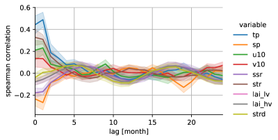
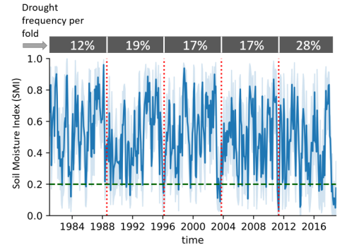
Figure 1: Left: Time-lagged Spearman correlation between the selected ERA5-Land input variables and the target variable SMI over 24 months. Right: Time series of SMI from 1981-2018 from the Helmholtz dataset. The shaded area shows the standard deviation across different locations. Red dotted lines show the split points for the time-based split into $k$ folds, and the green dashed line shows the binarization threshold for drought events. Shown above is the frequency of the positive class (drought events) per fold.

Low soil moisture levels depend on various meteorological input variables and the soil type. Retrieving accurate SMI ground-truth data is therefore complicated: Spatially-continuous soil moisture data on a resolution smaller than 0.25 degree is only available from satellite observations or model simulations. Satellite observations are exclusively available for recent years, include only the top few centimeters of the soil, and have data gaps due to unfavorable data retrieval conditions such as snow or dense vegetation [6]. Therefore, we select modeled SMI data as the ground-truth label. Due to SMI data availability, the selected experiment region is Germany. The data is limited to January 1981 to December 2018 by the availability of an overlapping period from both ERA5-Land and the SMI data. All datasets used in this study are freely available.

The target variable SMI is derived from the German drought monitor uppermost 25cm of soil data as SMI labels [30], which is generated by the hydrological model system based on data from about 2,500 weather stations [22, 13]. Figure 1 shows the SMI distribution over time and the chosen binarization threshold.

We use monthly time-series of 12 selected variables from the ERA5-Land reanalysis, e.g., pressure, precipitation, temperature (see Table A1). We selected ERA5-Land due to its higher resolution compared to ERA5 (9 km vs. 31 km) and its consequently better suitability for land applications [19]. To isolate the causal effects on SMI and avoid short-cut learning, we do not include potential confounding factors such as evaporation, runoff, and skin temperature. We also deliberately restrict the input variables to those commonly available in the latest generation of climate models to enable the transfer of the trained models to data directly obtained from climate model simulations.

Land use and vegetation type data based on the MODIS (MCD12Q1) Land Cover Data is used as an input feature, represented as soil type fractions [9].

Interpolation and Label Derivation Drought is an extreme weather event. Extreme events occur at the tail of variable distributions. Thus, we chose a classification setting with the tail of the SMI distribution as labels instead of a regression setting. The input data is re-gridded to the ERA5-Land regular latitude-longitude grid ($0.1^{\circ}\times 0.1^{\circ}\approx(9km)^{2}$). In this paper, we follow the drought classification from the German and U.S. drought monitors [27, 30] using an SMI threshold of $0.2$.

Dataset Split As seen in Figure 1, the SMI values for the same location exhibit a noticeable but declining correlation for lags up to 6 month. A simple random split over data points could therefore lead to data leakage, where memorizing SMI values from training and simple interpolation can lead to erroneously good results. Thus, we opt for a modified $k$-fold time-series split. First, we evenly determine $k-1$ split times to create $k$ time intervals. For the $k$th split, we train on folds $\{1,\ldots,k\}$, validate on fold $k+1$ and test on $k+2$. This split enables us to better assess parameter stability over time, mimicking increasing climate projection length. We decide to use $k=5$ as a good compromise between a sufficient number of folds for a robust performance estimate and large enough folds with multiple years of data to account for seasonal and interannual effects. Figure 1 shows the resulting folds separated by red dotted lines. Note that the drought sample availability (positive class) varies between folds from 12% to 28%.

3 Methodology

We frame drought classification as a binary classification problem given climate, land use as well as location data. Since the memory-effect [18] is suspected of playing an essential role in the development of droughts, we frame the problem as a sequence classification: The models use a window of the last $k$ months of climate input data for the current location to predict the drought label at the current time step. In addition to the climate variables, we also provide a positional and seasonal encoding as input features: For the positional encoding, we directly use the latitude & longitude grid values. A 2D circular encoding considers the seasonality based on the month of the year (month). $s=\left[\cos\left(2\pi\cdot\frac{\textit{month}}{12}\right);\sin\left(2\pi\cdot\frac{\textit{month}}{12}\right)\right]$, where $[\cdot;\cdot]$ denotes the concatenation. Besides using the location as an input feature, we do not explicitly include inductive biases for spatial correlation. Due to missing values and a non-rectangular shape of the available data area, simple grid-based methods such as a 2D-CNN are not directly applicable. The exploration of methods for irregular spatial data, such as those described in [4], will be a focus of future work.

Addressing Imbalanced Data In the entire dataset, examples for the drought class account for 18% of the total samples. We address this class imbalance by adding class weights proportional to the inverse class frequency during training and using an appropriate metric, PR-AUC, during evaluation.

Input Sequence Length The determination of a suitable sequence length is based on the Spearman correlation of the climate variables and the target SMI variable and the lagged correlation of the SMI variable, as both shown in Figure 1. Cyclical and non-cyclical decaying dependencies are considered, and both are indeed observed. Therefore, we select a window size of six months for our models, which in line with the period commonly used on monthly mean data by other drought indices such as the Standardized Precipitation Index (SPI) [17], and the Standardized Precipitation Evapotranspiration Index (SPEI) [29].

Models We investigate support vector machines (SVMs) (M1) with linear kernels as well as an MLP model which receives the flattened window as a single large vector as input (M2), which we denote by dense. To investigate whether an explicit inductive bias for sequential data is beneficial, we also include two main sequence encoders to obtain a representation of the input sequence for the sequence prediction. The cnn model (M3) applies multiple 1D convolutional layers before aggregating the input sequence to a single vector representation by average pooling. The lstm model (M4) uses multiple LSTM layers and the final hidden state as the sequence representation. For both sequence encoders, the drought classification is obtained by a fully connected layer on top of this representation.

Experimental Setup We use sklearn [21] for the SVM, and implement the other models in tensorflow [28]. To reflect the considerable class imbalance, we choose the area under the precision-recall curve (PR-AUC) as evaluation measure, which does not neglect the model’s performance for the minority/positive class, i.e., droughts. For hyperparameter optimization we use ray tune [15] with random search instead of grid search due to its higher efficiency [3]. The best hyperparameters are selected per fold according to validation PR-AUC on the fold’s validation data, and we report test results of the corresponding model trained across five different random seeds. The climate variables of the dataset are normalized to $[0,1]$.

4 Results and Discussion

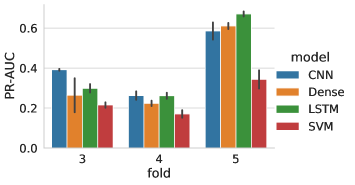
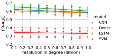
Figure 2: Left: Results on PR-AUC of the different models on the test dataset across five different random seeds for drought classification using a window of six months. Right: Ablation study:Inference on models trained on high resolution given input with decreasing resolution. Evaluation on five different random seeds using a window of six months.

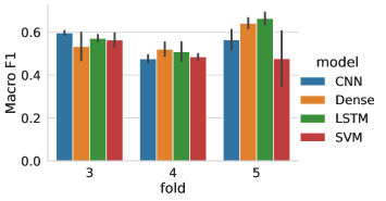
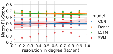
Figure A3: Left: Results on F1 Score of the different models on the test dataset across five different random seeds for drought classification using a window of six months. Right: Ablation study: Inference on models trained on high resolution given input with decreasing resolution. Evaluation on five different random seeds using a window of six months.

Model Comparison The resulting architectures were selected based on the validation PR-AUC on the second fold to account for a large variety of drought causes in the training data. The resulting hyperparameters are listed in Table A3. The results are shown in Figure 2, and Table A4. We observe that the PR-AUC is larger than the class frequency of the positive class indicating that the models indeed learned a non-trivial relation between the input variables and the target. The results for the F1 score can be found in Figure A3 with F1 scores larger than 0.5. Moreover, the performance varies for different folds, highlighting the challenging setting of a time-based split, where distributions can differ between different folds. There is no clear winner between the architectures: all models except the linear SVM perform comparable across folds. In particular, we do not observe a significant difference between models with an explicit inductive bias for sequential data. Since the utilized SMI data describes only the uppermost 25cm of the soil, the suspected memory effect might be more prominent in deeper soil layers. Our initial data analysis supports this, with the correlation of the input variables with the target being strongest close in time, cf. Figure 1.

Ablation: Coarsening the Data Resolution As an important future application of our models is on simulated climate data from climate models, we investigate further how the performance is affected by changing the resolution from the original $0.1^{\circ}$ to a coarser spatial resolution. The horizontal resolution of CMIP6 models varies from around 0.1^∘ to 2^∘ in the atmosphere [5]. Given the regional restriction of our input data, we restrict the ablation study to a range of 0.1^∘-1.0^∘ with 0.1^∘ steps. The architecture performing best on 0.1^∘ is used in inference to calculate the results on the coarser resolutions without re-training.

On the right-hand side of Figure 2 we visualize the results of the resolution ablation. In general, we observe a negative correlation between resolution and performance. The LSTM architecture is most affected by this but also generally shows the noisiest results overall. Overall, the models trained on 0.1^∘ input data show satisfactory performance when applied to coarser input data without dedicated training. This promising result indicates that it is possible to predict drought events under varying future climate scenarios with models trained on fine-grained drought labels.

5 Summary and Outlook

We summarize our contributions as follows: (1) We are the first to compare several ML models in their capability of classifying agricultural drought in a changing climate based on soil moisture index (SMI). We use ground truth data from a hydrological model and intentionally restrict the climate input variables to those available in the newest generation of CMIP6 climate models. We also include land use information. (2) We provide an ablation study regarding a transfer to coarser input data resolution, demonstrating that the model capabilities are transferable to lower resolution when trained in higher resolution.

In future work, we plan to use climate model output as input data for our algorithm to produce drought estimates under varying future scenarios. This will facilitate the transfer from learning on real input data to input data obtained from simulations. Apart from feeding the location information encoded as an additional input feature to the model, we plan to add location-aware models motivated by the strong regional correlation of the input variable as seen in Figure A4. Additionally, we plan to investigate other ground truth labels, e.g., SMAP [20] and expand the study region globally.

Overall, we consider our study as an important step towards machine learning-based agricultural drought detection. With our intentional restriction to variables available in climate models, we pave the way towards application on simulated data, thus facilitating the investigation of agricultural droughts in a changing climate.

Appendix

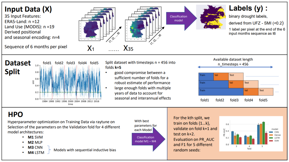
Figure A1: The first row displays the overall approach for classifying agricultural droughts by using a thresholded soil moisture index (SMI) from a hydrological model as ground truth labels per grid cell. Sequential input per location (6 months) are 35 input variables. The middle row shows the data split. We use a modified $k$-fold time-series split. The lower row displays the training and evaluation right and the hyperparameter optimization left as described in Section 3. The best hyperparameters are selected on the validation data. Due to the high imbalance in the dataset, for the evaluation, we use the area under the precision-recall curve (PR-AUC) metric to also focus on the model’s performance in correctly identifying the minority/positive class (drought). The evaluation results are reported on the test part of a split across five different random seeds.

Table A1: Overview of the variables used in this study. Native resolution of SMI: 4x4l, ERA5-Land: 9km, MODIS land use: 500mx500m

source	variable	description	unit
Helmholtz	SMI	soil moisture index topsoil (top25cm) via UFZ Drought Monitor	-
ERA5-Land	u10, v10	wind (u + v component at 10m)	$ms^{-1}$
	tp	total precipitation	$m$
	sp	surface pressure	$Pa$
	t2m	temperature	$K$
	ssrd	surface solar radiation downwards	$Jm^{-2}$
	d2m	dewpoint temperature	$K$
	ssr	surface net solar radiation	$Jm^{-2}$
	str	surface net thermal radiation	$Jm^{-2}$
	lai_lv, lai_hv	leaf area index high + low vegetation	$m^{2}m^{-2}$
	strd	surface thermal radiation downwards	$Jm^{-2}$
MODIS	land use class	water, evergreen needleleaf forest, Evergreen Broadleaf forest, Deciduous Needleleaf forest, Deciduous Broadleaf forest, Mixed forest, Closed shrublands, Open shrublands, Woody savannas, Savannas, Grasslands, Permanent wetlands, Croplands, Urban and built up, Cropland Natural vegetation mosaic, Snow and ice, Barren or sparsely vegetated, Cropland	Fraction
self-derived	positional encoding	latitude longitude grid	degree
self-derived	seasonal encoding	2D circular encoding of the month	degree

Table A2: Soil condition classification based on SMI according to [27, 30].

SMI	soil condition
$(0.2,\phantom{0}0.3\phantom{0}]$	abnormally dry
$(0.1,\phantom{0}0.2\phantom{0}]$	moderate drought
$(0.05,0.1\phantom{0}]$	severe drought
$(0.02,0.05]$	extreme drought
$(0,\phantom{.00}0.02]$	exceptional drought

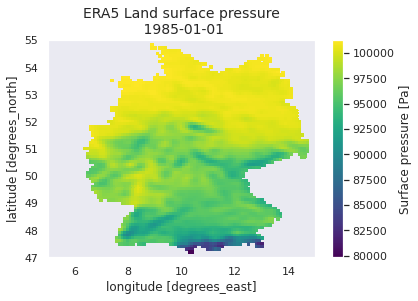
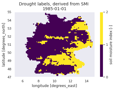
Figure A2: Data examples for 1 month. Left: ERA5 input variable example "pressure" Right: Target variable: Binarized SMI

Table A3: The Hyperparameters resulting from the random search for binary drought classification.

type	HPO fold	hidden	lr	dropout	activation	batchnorm	batch size
LSTM	2	16, 32	$1.18\text{e-}4$	0.1	softplus	False	2208
	3	96, 96	$1.00\text{e-}4$	0.2	relu	False	96
	4	32, 48, 128	$2.15\text{e-}5$	0.0	softplus	True	2592
CNN	2	128, 176, 224, 240	$3.53\text{e-}5$	0.1	softplus	False	32
	3	112, 176	$2.40\text{e-}5$	0.2	softplus	False	64
	4	16, 96, 128	$1.29\text{e-}2$	0.1	ReLu	True	448
Dense	2	32, 48, 96	$3.36\text{e-}2$	0.1	relu	False	769
	3	48, 208, 208, 208	$1.66\text{e-}2$	0.2	softplus	True	192
	4	80, 192	$1.02\text{e-}5$	0.2	ReLu	True	800

Table A4: Results on the test dataset across five different random seeds for drought classification using a window of six months.

		Macro F1		PR-AUC
		mean	std	mean	std
model	test fold
dense	3	0.5340	0.0724	0.2640	0.0950
	4	0.5212	0.0359	0.2234	0.0148
	5	0.6424	0.0272	0.6106	0.0170
lstm	3	0.5722	0.0176	0.2986	0.0236
	4	0.5096	0.0494	0.2614	0.0168
	5	0.6648	0.0311	0.6708	0.0138
cnn	3	0.5976	0.0101	0.3914	0.0050
	4	0.4766	0.0189	0.2624	0.0235
	5	0.5650	0.0520	0.5854	0.0480
SVM	3	0.5642	0.0352	0.2150	0.0150
	4	0.4858	0.0154	0.1704	0.0210
	5	0.4772	0.1437	0.3432	0.0508

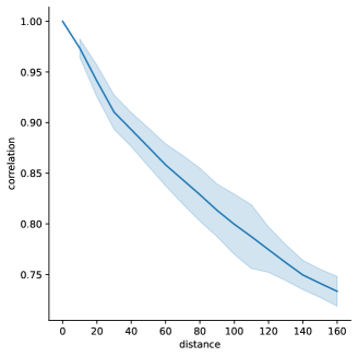
Figure A4: Time-lagged Spearman autocorrelation for the SMI target variable at the same location. The shaded area shows the standard deviation of the Spearman correlation across all analyzed locations.

References

- Belayneh et al. [2016] Belayneh, A., Adamowski, J., Khalil, B., and Quilty, J. Coupling machine learning methods with wavelet transforms and the bootstrap and boosting ensemble approaches for drought prediction. Atmospheric Research, 172-173:37–47, 2016. ISSN 0169-8095. doi: https://doi.org/10.1016/j.atmosres.2015.12.017. URL https://www.sciencedirect.com/science/article/pii/S016980951600003X.
- Below et al. [2007] Below, R., Grover-Kopec, E., and Dilley, M. Documenting drought-related disasters: A global reassessment. The Journal of Environment & Development, 16(3):328–344, 2007.
- Bergstra & Bengio [2012] Bergstra, J. and Bengio, Y. Random search for hyper-parameter optimization. J. Mach. Learn. Res., 13(null):281–305, February 2012.
- Bronstein et al. [2017] Bronstein, M. M., Bruna, J., LeCun, Y., Szlam, A., and Vandergheynst, P. Geometric deep learning: Going beyond euclidean data. IEEE Signal Process. Mag., 34(4):18–42, 2017. doi: 10.1109/MSP.2017.2693418. URL https://doi.org/10.1109/MSP.2017.2693418.
- Cannon [2020] Cannon, A. J. Reductions in daily continental-scale atmospheric circulation biases between generations of global climate models: CMIP5 to CMIP6. Environmental Research Letters, 15(6):064006, May 2020. doi: 10.1088/1748-9326/ab7e4f. URL https://doi.org/10.1088/1748-9326/ab7e4f.
- Dorigo et al. [2017] Dorigo, W., Wagner, W., Albergel, C., Albrecht, F., Balsamo, G., Brocca, L., Chung, D., Ertl, M., Forkel, M., Gruber, A., Haas, E., Hamer, P. D., Hirschi, M., Ikonen, J., de Jeu, R., Kidd, R., Lahoz, W., Liu, Y. Y., Miralles, D., Mistelbauer, T., Nicolai-Shaw, N., Parinussa, R., Pratola, C., Reimer, C., van der Schalie, R., Seneviratne, S. I., Smolander, T., and Lecomte, P. ESA CCI soil moisture for improved earth system understanding: State-of-the art and future directions. Remote Sensing of Environment, 203:185–215, December 2017. doi: 10.1016/j.rse.2017.07.001. URL https://doi.org/10.1016/j.rse.2017.07.001.
- Eyring et al. [2016] Eyring, V., Bony, S., Meehl, G. A., Senior, C. A., Stevens, B., Stouffer, R. J., and Taylor, K. E. Overview of the coupled model intercomparison project phase 6 (CMIP6) experimental design and organization. Geoscientific Model Development, 9(5):1937–1958, May 2016. doi: 10.5194/gmd-9-1937-2016. URL https://doi.org/10.5194/gmd-9-1937-2016.
- Feng et al. [2019] Feng, P., Wang, B., Liu, D. L., and Yu, Q. Machine learning-based integration of remotely-sensed drought factors can improve the estimation of agricultural drought in south-eastern australia. Agricultural Systems, 173:303–316, 2019. ISSN 0308-521X. doi: https://doi.org/10.1016/j.agsy.2019.03.015. URL https://www.sciencedirect.com/science/article/pii/S0308521X18314021.
- Friedl & Sulla-Menashe [2019] Friedl, M. and Sulla-Menashe, D. MCD12Q1 MODIS/Terra+Aqua Land Cover Type Yearly L3 Global 500m SIN Grid V006, 2019. URL https://lpdaac.usgs.gov/products/mcd12q1v006/. type: dataset.
- Keyantash & Dracup [2002] Keyantash, J. and Dracup, J. A. The quantification of drought: an evaluation of drought indices. Bulletin of the American Meteorological Society, 83(8):1167–1180, 2002.
- King et al. [2020] King, A. D., Pitman, A. J., Henley, B. J., Ukkola, A. M., and Brown, J. R. The role of climate variability in australian drought. Nature Climate Change, 10(3):177–179, February 2020. doi: 10.1038/s41558-020-0718-z. URL https://doi.org/10.1038/s41558-020-0718-z.
- Kratzert et al. [2018] Kratzert, F., Klotz, D., Brenner, C., Schulz, K., and Herrnegger, M. Rainfall–runoff modelling using long short-term memory (lstm) networks. Hydrology and Earth System Sciences, 22(11):6005–6022, 2018.
- Kumar et al. [2013] Kumar, R., Samaniego, L., and Attinger, S. Implications of distributed hydrologic model parameterization on water fluxes at multiple scales and locations. Water Resources Research, 49(1):360–379, January 2013. doi: 10.1029/2012wr012195. URL https://doi.org/10.1029/2012wr012195.
- Le et al. [2019] Le, X.-H., Ho, H. V., Lee, G., and Jung, S. Application of long short-term memory (lstm) neural network for flood forecasting. Water, 11(7):1387, 2019.
- Liaw et al. [2018] Liaw, R., Liang, E., Nishihara, R., Moritz, P., Gonzalez, J. E., and Stoica, I. Tune: A research platform for distributed model selection and training. arXiv preprint arXiv:1807.05118, 2018.
- Lloyd-Hughes [2013] Lloyd-Hughes, B. The impracticality of a universal drought definition. Theoretical and Applied Climatology, 117(3-4):607–611, October 2013. doi: 10.1007/s00704-013-1025-7. URL https://doi.org/10.1007/s00704-013-1025-7.
- McKee et al. [1993] McKee, T. B., Doesken, N. J., Kleist, J., et al. The relationship of drought frequency and duration to time scales. In Proceedings of the 8th Conference on Applied Climatology, volume 17, pp. 179–183. Boston, 1993.
- Mo [2011] Mo, K. C. Drought onset and recovery over the united states. Journal of Geophysical Research: Atmospheres, 116(D20), 2011. doi: https://doi.org/10.1029/2011JD016168. URL https://agupubs.onlinelibrary.wiley.com/doi/abs/10.1029/2011JD016168.
- Muñoz-Sabater et al. [2021] Muñoz-Sabater, J., Dutra, E., Agustí-Panareda, A., Albergel, C., Arduini, G., Balsamo, G., Boussetta, S., Choulga, M., Harrigan, S., Hersbach, H., Martens, B., Miralles, D. G., Piles, M., Rodríguez-Fernández, N. J., Zsoter, E., Buontempo, C., and Thépaut, J.-N. ERA5-land: A state-of-the-art global reanalysis dataset for land applications. March 2021. doi: 10.5194/essd-2021-82. URL https://doi.org/10.5194/essd-2021-82.
- ONeill et al. [2020] ONeill, P. E., Chan, S., Njoku, E. G., Jackson, T., Bindlish, R., and Chaubell, M. J. Smap enhanced l3 radiometer global daily 9 km ease-grid soil moisture, version 4, 2020. URL https://nsidc.org/data/SPL3SMP_E/versions/4.
- Pedregosa et al. [2011] Pedregosa, F., Varoquaux, G., Gramfort, A., Michel, V., Thirion, B., Grisel, O., Blondel, M., Prettenhofer, P., Weiss, R., Dubourg, V., et al. Scikit-learn: Machine learning in python. Journal of machine learning research, 12(Oct):2825–2830, 2011.
- Samaniego et al. [2010] Samaniego, L., Kumar, R., and Attinger, S. Multiscale parameter regionalization of a grid-based hydrologic model at the mesoscale. Water Resources Research, 46(5), May 2010. doi: 10.1029/2008wr007327. URL https://doi.org/10.1029/2008wr007327.
- Samaniego et al. [2018] Samaniego, L., Thober, S., Kumar, R., Wanders, N., Rakovec, O., Pan, M., Zink, M., Sheffield, J., Wood, E. F., and Marx, A. Anthropogenic warming exacerbates european soil moisture droughts. Nature Climate Change, 8(5):421–426, April 2018. doi: 10.1038/s41558-018-0138-5. URL https://doi.org/10.1038/s41558-018-0138-5.
- Seneviratne et al. [2021] Seneviratne, S. I., X. Zhang, M., Adnan, W. B., Dereczynski, C., Luca, A. D., Ghosh, S., Iskandar, I., Kossin, J., Lewis, S., F. Otto, I., Pinto, M. S., Vicente-Serrano, S. M., and Zhou, M. W. B. Weather and climate extreme events in a changing climate. Climate Change 2021: The Physical Science Basis. Contribution of Working Group I to the Sixth Assessment Report of the Intergovernmental Panel on Climate Change, 2021.
- Shamshirband et al. [2020] Shamshirband, S., Hashemi, S., Salimi, H., Samadianfard, S., Asadi, E., Shadkani, S., Kargar, K., Mosavi, A., Nabipour, N., and Chau, K.-W. Predicting standardized streamflow index for hydrological drought using machine learning models. Engineering Applications of Computational Fluid Mechanics, 14(1):339–350, January 2020. doi: 10.1080/19942060.2020.1715844. URL https://doi.org/10.1080/19942060.2020.1715844.
- Sheffield & Wood [2007] Sheffield, J. and Wood, E. F. Characteristics of global and regional drought, 1950–2000: Analysis of soil moisture data from off-line simulation of the terrestrial hydrologic cycle. Journal of Geophysical Research: Atmospheres, 112(D17), 2007.
- Svoboda et al. [2002] Svoboda, M., LeComte, D., Hayes, M., Heim, R., Gleason, K., Angel, J., Rippey, B., Tinker, R., Palecki, M., Stooksbury, D., et al. The drought monitor. Bulletin of the American Meteorological Society, 83(8):1181–1190, 2002.
- TensorFlow Developers [2021] TensorFlow Developers. Tensorflow, 2021. URL https://zenodo.org/record/4758419.
- Vicente-Serrano et al. [2010] Vicente-Serrano, S. M., Beguería, S., and López-Moreno, J. I. A multiscalar drought index sensitive to global warming: The standardized precipitation evapotranspiration index. Journal of Climate, 23(7):1696–1718, April 2010. doi: 10.1175/2009jcli2909.1. URL https://doi.org/10.1175/2009jcli2909.1.
- Zink et al. [2016] Zink, M., Samaniego, L., Kumar, R., Thober, S., Mai, J., Schäfer, D., and Marx, A. The german drought monitor. Environmental Research Letters, 11(7):074002, 2016.