A structure preserving front tracking finite element method for the Mullins–Sekerka problem

Abstract

We introduce and analyse a fully discrete approximation for a mathematical model for the solidification and liquidation of materials of negligible specific heat. The model is a two-sided Mullins–Sekerka problem. The discretization uses finite elements in space and an independent parameterization of the moving free boundary. We prove unconditional stability and exact volume conservation for the introduced scheme. Several numerical simulations, including for nearly crystalline surface energies, demonstrate the practicality and accuracy of the presented numerical method.

Key words. Mullins–Sekerka, Hele–Shaw, anisotropy, parametric finite element method, unconditional stability, volume preservation

AMS subject classifications. 35K55, 35R35, 65M12, 65M50, 65M60, 74E10, 74E15, 80A22

1 Introduction

In this paper we propose and analyse a novel numerical approximation of the following moving boundary problem. Let $\Omega\subset{\mathbb{R}}^{d}$, $d\geq 2$, be a domain with a Lipschitz boundary $\partial\Omega$ and outer unit normal $\vec{\nu}_{\Omega}$. Given the hypersurface $\Gamma(0)\subset\Omega$, find $u:\Omega\times[0,T]\to{\mathbb{R}}$ and the evolving hypersurface $(\Gamma(t))_{t\in[0,T]}$ such that for all $t\in(0,T]$ the following conditions hold:

$$-\Delta u =0\quad \text{in }\Omega\setminus\Gamma(t),$$ (1.1a)

$$u =\varkappa\quad \text{on }\Gamma(t),$$ (1.1b)

$$\left[\frac{\partial u}{\partial{\vec{\nu}}}\right]_{\Gamma(t)} =-\mathcal{V}\quad \text{on }\Gamma(t),$$ (1.1c)

$$\frac{\partial u}{\partial{\vec{\nu}_{\Omega}}} =0\quad \text{on }\partial\Omega,$$ (1.1d)

where $\vec{\nu}$ is the outer unit normal of $\Gamma(t)$, $\varkappa$ is its mean curvature, $[\cdot]_{\Gamma(t)}$ denotes the jump of a quantity across the interface $\Gamma(t)$ and $\mathcal{V}$ is the normal velocity of $(\Gamma(t))_{t\in[0,T]}$. Here our sign convention is such that the unit sphere has mean curvature $\varkappa=1-d<0$.

The problem (1.1) is usually called the Mullins–Sekerka problem, or the two-sided Mullins–Sekerka flow, and geometrically it can be viewed as a prototype for a curvature driven interface evolution that involves quantities defined in the bulk regions surrounding the interface. Alternative names for (1.1) in the literature are Hele–Shaw flow with surface tension, or quasi-static Stefan problem. For theoretical results on the existence of strong and weak solutions to (1.1) we refer to [19, 20, 26] and the references therein. Physically, the system (1.1) was derived as a model for solidification and liquidation of materials of negligible specific heat, [33]. In addition, the Mullins–Sekerka problem arises as the sharp interface limit of the non-degenerate Cahn–Hilliard equation, as was proved in [1]. Here we recall that the Cahn–Hilliard equation models the process of phase separation and coarsening in melted alloys, [16].

As regards the numerical approximation of the Mullins–Sekerka problem (1.1), several different approaches are available from the literature. Approximations based on a boundary integral formulation can be found in e.g. [14, 37, 32], while a front-tracking method based on parametric finite elements has been proposed in [7]. For a finite difference approximation of a levelset formulation we refer to [18], while finite element approximations of phasefield models have been considered in [28, 27, 9, 10]. In this paper we will consider a front-tracking method, where the numerical approximation of the interface $\Gamma(t)$ is completely independent of the finite element mesh for the bulk equation (1.1a). In fact, we will propose an improvement for the unfitted finite element approximation that was introduced by the author together with John W. Barrett and Harald Garcke in [7]. Here we will put particular emphasis on the conservation of physically relevant properties on the discrete level.

By way of motivation, we observe that it is not difficult to prove that a solution to the Mullins–Sekerka problem (1.1) reduces the surface area $|\Gamma(t)|$, while it maintains the volume of the enclosed domain $\Omega_{-}(t)$. In particular, it holds that

$$\frac{\rm d}{{\rm d}t}|\Gamma(t)|=\frac{\rm d}{{\rm d}t}\int_{\Gamma(t)}1\;{\rm d}{\mathcal{H}}^{d-1}=-\int_{\Gamma(t)}\varkappa\mathcal{V}\;{\rm d}{\mathcal{H}}^{d-1}=-\int_{\Omega}|\nabla u|^{2}\;{\rm d}{\mathcal{L}}^{d}\leq 0$$ (1.2)

and

$$\frac{\rm d}{{\rm d}t}\operatorname{vol}(\Omega_{-}(t))=\int_{\Gamma(t)}\mathcal{V}\;{\rm d}{\mathcal{H}}^{d-1}=0,$$ (1.3)

see e.g. Remark 105 in [13]. We remark that these properties motivate the interpretation of (1.1) as a volume preserving gradient flow of the surface area. Examples for volume preserving gradient flows of the surface area that only depend on geometric properties of the interface are the conserved mean curvature flow and surface diffusion, [17, 35]. In contrast, the flow (1.1) also depends on the field $u$ that is defined in the bulk. A detailed description of the gradient flow structure for (1.1) can be found in [7, Appendix A]. Clearly, for a numerical approximation of (1.1) it would be highly desirable to have a discrete analogue of the energy dissipation law (1.2) and the volume conservation property (1.3). The fully discrete method from [7] satisfies a discrete analogue of (1.2), in particular it is unconditionally stable. But a discrete version of (1.3) does not hold. That means that for large time steps, and in certain situations, a significant loss of mass can be observed in computations. On utilizing very recent ideas from [30, 3], we will appropriately adapt the fully discrete scheme from [7] to obtain a new method for (1.1) that satisfies discrete analogues of both (1.2) and (1.3). We believe this is the first such fully discrete approximation of (1.1) in the literature.

In many physical applications, e.g. when considering the solidification or liquidation of materials, the density of the interfacial energy is directionally dependent. A typical example for such an anisotropic surface energy is

$$|\Gamma(t)|_{\gamma}=\int_{\Gamma(t)}\gamma(\vec{\nu})\;{\rm d}{\mathcal{H}}^{d-1},$$ (1.4)

where $\gamma$ is a given anisotropy function. We refer to [36, 15, 23, 29] for more details on anisotropic surface energies. On defining the anisotropic mean curvature $\varkappa_{\gamma}$ as the first variation of (1.4), so that e.g. $\frac{\rm d}{{\rm d}t}|\Gamma(t)|_{\gamma}=-\int_{\Gamma(t)}\varkappa_{\gamma}\mathcal{V}\;{\rm d}{\mathcal{H}}^{d-1}$, we can introduce the anisotropic Mullins–Sekerka problem by replacing $\varkappa$ with $\varkappa_{\gamma}$ in (1.1). Then the energy dissipation (1.2) and volume conservation (1.3) hold as before, where of course in the former we need to replace $|\Gamma(t)|$ with $|\Gamma(t)|_{\gamma}$ and $\varkappa$ with $\varkappa_{\gamma}$. The numerical method we discuss in this paper, by virtue of being derived from the scheme in [7], can deal with the anisotropic Mullins–Sekerka problem as well. In addition, for a class of anisotropies that was first proposed in [4, 6], the anisotropic scheme will still be structure preserving, in the sense that discrete analogues of the anisotropic (1.2) and (1.3) will hold.

In summary, the novel fully practical and fully discrete numerical method proposed in this paper has the following properties:

• The method is unconditionally stable, i.e. it mimics (1.2) on the discrete level.

• The volume of the two phases, i.e. the interior and the exterior of the interface, is conserved exactly, as a fully discrete analogue to (1.3).

• The polyhedral interface approximation maintains a nice mesh property, leading to asymptotically equidistributed polygonal curves in the case $d=2$ for an isotropic surface energy.

• The method is unfitted, meaning mesh deformations of the bulk mesh are avoided, and no remeshings of the bulk triangulation are necessary.

• The method can take an anisotropic surface energy into account, meaning that a discrete analogue of the anisotropic generalization of (1.2) still holds on the fully discrete level.

The remainder of the paper is organized as follows. In Section 2 we introduce a weak formulation for the Mullins–Sekerka problem (1.1) on which our finite element method is going be based. We also state a semidiscrete continuous-in-time approximation and briefly analyse its properties. Our novel fully discrete finite element approximation is presented and analysed in Section 3, where in order to focus on the structure preserving aspect of the method, we at first concentrate on the isotropic case. Subsequently, in Section 4, we discuss the extension of the weak formulation and the finite element scheme to the anisotropic case. Finally, in Section 5 we consider several numerical simulations for the introduced numerical method, including some convergence experiments.

2 Weak formulation and semidiscrete approximation

Our parametric finite element method will be based on a suitable weak formulation of (1.1), which we introduce in this section. Here we follow the notation and presentation from the recent review article [13].

Let

$${\mathcal{G}_{T}}=\bigcup_{t\in[0,T]}(\Gamma(t)\times\{t\})$$

be a smooth evolving hypersurface, such that for every $t\in[0,T]$ the closed hypersurface $\Gamma(t)\subset\Omega$ partitions the domain $\Omega$ into two phases: the interior $\Omega_{-}(t)$ and the exterior $\Omega_{+}(t)=\Omega\setminus\overline{\Omega_{-}(t)}$, so that $\partial\Omega_{-}(t)=\Gamma(t)$. In what follows, we will often not distinguish between $\Gamma(t)\times\{t\}$ and $\Gamma(t)$. Moreover, as we are interested in a parametric formulation of the evolving interface, we assume that $\vec{x}:\Upsilon\times[0,T]\to{\mathbb{R}}^{d}$ is a global parameterization of $(\Gamma(t))_{t\in[0,T]}$, where $\Upsilon\subset{\mathbb{R}}^{d}$ is a smooth reference manifold. We recall that the induced full velocity of $\Gamma(t)$ is defined by

$$\vec{\mathcal{V}}(\vec{x}(\vec{q},t),t)=(\partial_{t}\vec{x})(\vec{q},t)\quad\forall\ (\vec{q},t)\in\Upsilon\times[0,T],$$

and satisfies $\vec{\mathcal{V}}\cdot\vec{\nu}=\mathcal{V}$. Multiplying (1.1a) with a test function $\phi\in H^{1}(\Omega)$, integrating over $\Omega$ and performing integration by parts yields

$$0=\int_{\Omega_{-}(t)\cup\Omega_{+}(t)}\phi\Delta u\;{\rm d}{\mathcal{L}}^{d}=\int_{\partial\Omega}\phi\frac{\partial u}{\partial\vec{\nu}_{\Omega}}\;{\rm d}{\mathcal{H}}^{d-1}-\int_{\Gamma(t)}\phi\left[\frac{\partial u}{\partial\vec{\nu}}\right]_{\Gamma(t)}\;{\rm d}{\mathcal{H}}^{d-1}-\int_{\Omega}\nabla u\cdot\nabla\phi\;{\rm d}{\mathcal{L}}^{d},$$

which in view of the conditions (1.1c) and (1.1d) reduces to

$$0=\int_{\Gamma(t)}\phi\mathcal{V}\;{\rm d}{\mathcal{H}}^{d-1}-\int_{\Omega}\nabla u\cdot\nabla\phi\;{\rm d}{\mathcal{L}}^{d}.$$

The only other ingredient needed for the weak formulation is the well-known variational formulation of mean curvature, given by

$$\int_{\Gamma(t)}\varkappa\vec{\eta}\cdot\vec{\nu}+\nabla_{\!s}\vec{\rm id}:\nabla_{\!s}\vec{\eta}\;{\rm d}{\mathcal{H}}^{d-1}=0\qquad\vec{\eta}\in[H^{1}(\Gamma(t))]^{d},$$ (2.1)

where $\vec{\rm id}$ denotes the identity function in ${\mathbb{R}}^{d}$ and $\nabla_{\!s}$ is the surface gradient on $\Gamma(t)$, see e.g. Remark 22 in [13]. Hence, on denoting the $L^{2}$–inner products over $\Omega$ and $\Gamma(t)$ by $(\cdot,\cdot)$ and $\langle\cdot,\cdot\rangle_{\Gamma(t)}$, respectively, we can state the weak formulation as follows.

Given a closed hypersurface $\Gamma(0)\subset\Omega$, we seek an evolving hypersurface $(\Gamma(t))_{t\in[0,T]}$ that separates $\Omega$ into $\Omega_{-}(t)$ and $\Omega_{+}(t)$, with a global parameterization and induced velocity field $\vec{\mathcal{V}}$, and $\varkappa:L^{2}({\mathcal{G}_{T}})$ as well as $u:\Omega\times[0,T]\to{\mathbb{R}}$, such that for almost all $t\in(0,T)$ it holds for $(u(\cdot,t),\vec{\mathcal{V}}(\cdot,t),\varkappa(\cdot,t))\in H^{1}(\Omega)\times[L^{2}(\Gamma(t))]^{d}\times L^{2}(\Gamma(t))$ that

$$\left(\nabla u,\nabla\phi\right)-\left\langle\vec{\mathcal{V}},\phi\vec{\nu}\right\rangle_{\Gamma(t)} =0\qquad\forall\ \phi\in H^{1}(\Omega),$$ (2.2a)

$$\left\langle u-\varkappa,\chi\right\rangle_{\Gamma(t)} =0\qquad\forall\ \chi\in L^{2}(\Gamma(t)),$$ (2.2b)

$$\left\langle\varkappa\vec{\nu},\vec{\eta}\right\rangle_{\Gamma(t)}+\left\langle\nabla_{\!s}\vec{\rm id},\nabla_{\!s}\vec{\eta}\right\rangle_{\Gamma(t)} =0\qquad\forall\ \vec{\eta}\in[H^{1}(\Gamma(t))]^{d}.$$ (2.2c)

Clearly, choosing $\phi=u$ in (2.2a) and $\chi=\mathcal{V}=\vec{\mathcal{V}}\cdot\vec{\nu}$ in (2.2b) yields the energy dissipation law (1.2), while choosing $\phi=1$ in (2.2a) leads to the volume conservation property (1.3). Mimicking these testing procedures on the discrete level will be crucial to prove the structure preserving aspect of our finite element approximations.

For the numerical approximation of (2.2) we first introduce the necessary finite element space in the bulk. To this end, we assume that $\Omega$ is a polyhedral domain. Then let $\mathcal{T}^{h}$ be a regular partitioning of $\Omega$ into disjoint open simplices, so that $\overline{\Omega}=\cup_{o\in\mathcal{T}^{h}}\overline{o}$, see [21]. Associated with $\mathcal{T}^{h}$ is the finite element space

$$S^{h}=\left\{\chi\in C^{0}(\overline{\Omega}):\chi_{\mid_{o}}\text{ is affine }\forall\ o\in\mathcal{T}^{h}\right\}\subset H^{1}(\Omega).$$ (2.3)

In addition we need appropriate parametric finite element spaces. Let a polyhedral hypersurface $\Gamma^{h}\subset{\mathbb{R}}^{d}$ be given by

$$\Gamma^{h}=\bigcup_{j=1}^{J}\overline{\sigma_{j}},$$ (2.4)

where $\{\sigma_{j}\}_{j=1}^{J}$ is a family of disjoint, (relatively) open $(d-1)$-simplices, such that $\overline{\sigma_{i}}\cap\overline{\sigma_{j}}$ for $i\not=j$ is either empty or a common $k$-simplex of $\overline{\sigma_{i}}$ and $\overline{\sigma_{j}}$, $0\leq k<d$. We denote the vertices of $\Gamma^{h}$ by $\{\vec{q}_{k}\}_{k=1}^{K}$, and assume that the vertices of $\sigma_{j}$ are given by $\{\vec{q}_{j,k}\}_{k=1}^{d}$, $j=1,\ldots,J$. Here the numbering of the local vertices is assumed to be such that

$$\vec{\nu}^{h}=\frac{(\vec{q}_{j,2}-\vec{q}_{j,1})\land\cdots\land(\vec{q}_{j,d}-\vec{q}_{j,1})}{|(\vec{q}_{j,2}-\vec{q}_{j,1})\land\cdots\land(\vec{q}_{j,d}-\vec{q}_{j,1})|}\qquad\text{on }\sigma_{j},\quad j=1,\ldots,J,$$ (2.5)

defines the outer normal $\vec{\nu}^{h}\in[L^{\infty}(\Gamma^{h})]^{d}$ to the interior $\Omega^{h}_{-}$ of $\Gamma^{h}=\partial\Omega^{h}_{-}$. Here we recall the definition of the wedge product from [13, Definition 45], i.e. for $\vec{v}_{1},\ldots,\vec{v}_{d-1}\in{\mathbb{R}}^{d}$, the wedge product is the unique vector such that $\vec{b}\cdot(\vec{v}_{1}\land\cdots\land\vec{v}_{d-1})=\det(\vec{v}_{1},\ldots,\vec{v}_{d-1},\vec{b})$ for all $\vec{b}\in{\mathbb{R}}^{d}$. It follows that it is the usual cross product of two vectors in ${\mathbb{R}}^{3}$, and the anti-clockwise rotation through $\frac{\pi}{2}$ of a vector in ${\mathbb{R}}^{2}$. We note also that

$$|\sigma_{j}|=\frac{1}{d-1}|(\vec{q}_{j,2}-\vec{q}_{j,1})\land\cdots\land(\vec{q}_{j,d}-\vec{q}_{j,1})|.$$ (2.6)

We define the finite element spaces of continuous piecewise linear functions on $\Gamma^{h}$ via

$$V(\Gamma^{h})=\{\chi\in C^{0}(\Gamma^{h}):\chi_{\mid_{\sigma_{j}}}\text{ is affine for $j=1,\ldots,J$}\}\quad\text{and}\quad\underline{V}(\Gamma^{h})=[V(\Gamma^{h})]^{d}.$$

We let $\{\phi^{\Gamma^{h}}_{k}\}_{k=1}^{K}$ denote the standard basis of $V(\Gamma^{h})$, i.e.

$$\phi^{\Gamma^{h}}_{i}(\vec{q}_{j})=\delta_{ij},\qquad i,j=1,\ldots,K.$$

Moreover, we let $\pi_{\Gamma^{h}}:C^{0}(\Gamma^{h})\to V(\Gamma^{h})$ be the standard interpolation operator, and let $\left\langle\cdot,\cdot\right\rangle_{\Gamma^{h}}$ denote the $L^{2}$–inner product on $\Gamma^{h}$. For two piecewise continuous functions $u,v\in L^{\infty}(\Gamma^{h})$, with possible jumps across the edges of $\{\sigma_{j}\}_{j=1}^{J}$, we introduce the mass lumped inner product $\left\langle\cdot,\cdot\right\rangle^{h}_{\Gamma^{h}}$ as

$$\left\langle u,v\right\rangle^{h}_{\Gamma^{h}}=\frac{1}{d}\sum_{j=1}^{J}|\sigma_{j}|\sum_{k=1}^{d}(uv)((\vec{q}_{j,k})^{-}),$$ (2.7)

where $u((\vec{q})^{-})=\underset{\sigma_{j}\ni\vec{p}\to\vec{q}}{\lim}u(\vec{p})$. The definition (2.7) is naturally extended to vector- and tensor-valued functions. On recalling (2.5), we define the vertex normal vector $\vec{\omega}^{h}\in\underline{V}(\Gamma^{h})$ to be the mass-lumped $L^{2}$–projection of $\vec{\nu}^{h}$ onto $\underline{V}(\Gamma^{h})$, i.e.

$$\left\langle\vec{\omega}^{h},\vec{\varphi}\right\rangle_{\Gamma^{h}}^{h}=\left\langle\vec{\nu}^{h},\vec{\varphi}\right\rangle_{\Gamma^{h}}\quad\forall\ \vec{\varphi}\in\underline{V}(\Gamma^{h}).$$ (2.8)

From now on, we let

$${\mathcal{G}^{h}_{T}}=\bigcup_{t\in[0,T]}(\Gamma^{h}(t)\times\{t\})$$

be an evolving polyhedral hypersurface, so that $\Gamma^{h}(t)$, for each $t\in[0,T]$, is a polyhedral surface of the form (2.4) for fixed $J$ and $K$. That is, $\Gamma^{h}(t)$ is defined through its elements $\{\sigma^{h}_{j}(t)\}_{j=1}^{J}$ and its vertices $\{\vec{q}^{h}_{k}(t)\}_{k=1}^{K}$. We will often not distinguish between ${\mathcal{G}^{h}_{T}}$ and $(\Gamma^{h}(t))_{t\in[0,T]}$. Then the full velocity of $\Gamma^{h}(t)$ is defined by

$$\vec{\mathcal{V}}^{h}(\vec{z},t)=\sum_{k=1}^{K}\left[\frac{\rm d}{{\rm d}t}\vec{q}_{k}(t)\right]\phi^{\Gamma^{h}(t)}_{k}(\vec{z})\quad\forall\ (\vec{z},t)\in{\mathcal{G}^{h}_{T}}.$$ (2.9)

We also define the finite element spaces

$$V({\mathcal{G}^{h}_{T}})=\{\chi\in C^{0}({\mathcal{G}^{h}_{T}}):\chi(\cdot,t)\in V(\Gamma^{h}(t))\quad\forall\ t\in[0,T]\}\quad\text{and}\quad\underline{V}({\mathcal{G}^{h}_{T}})=[V({\mathcal{G}^{h}_{T}})]^{d}.$$

Our unfitted semidiscrete finite element approximation of (2.2) can then be formulated as follows. Given the closed polyhedral hypersurface $\Gamma^{h}(0)$, find an evolving polyhedral hypersurface $(\Gamma^{h}(t))_{t\in[0,T]}$, that separates $\Omega$ into $\Omega^{h}_{-}(t)$ and $\Omega^{h}_{+}(t)$, with induced velocity $\vec{\mathcal{V}}^{h}\in\underline{V}({\mathcal{G}^{h}_{T}})$, and $\kappa^{h}\in V({\mathcal{G}^{h}_{T}})$ as well as $u^{h}\in S^{h}\times(0,T]$, such that for all $t\in(0,T]$ it holds for $(u^{h}(\cdot,t),\vec{\mathcal{V}}^{h}(\cdot,t),\kappa^{h}(\cdot,t))\in S^{h}\times\underline{V}(\Gamma^{h}(t))\times V(\Gamma^{h}(t))$ that

$$\left(\nabla u^{h},\nabla\phi\right)-\left\langle\pi_{\Gamma^{h}(t)}\left[\vec{\mathcal{V}}^{h}\cdot\vec{\omega}^{h}\right],\phi\right\rangle_{\Gamma^{h}(t)}^{(h)} =0\qquad\forall\ \phi\in S^{h},$$ (2.10a)

$$\left\langle u^{h},\chi\right\rangle_{\Gamma^{h}(t)}^{(h)}-\left\langle\kappa^{h},\chi\right\rangle_{\Gamma^{h}(t)}^{h} =0\qquad\forall\ \chi\in V(\Gamma^{h}(t)),$$ (2.10b)

$$\left\langle\kappa^{h}\vec{\omega}^{h},\vec{\eta}\right\rangle_{\Gamma^{h}(t)}^{h}+\left\langle\nabla_{\!s}\vec{\rm id},\nabla_{\!s}\vec{\eta}\right\rangle_{\Gamma^{h}(t)} =0\qquad\forall\ \vec{\eta}\in\underline{V}(\Gamma^{h}(t)),$$ (2.10c)

where the surface gradients $\nabla_{\!s}$ in (2.10c) are defined piecewise on the polyhedral surface $\Gamma^{h}(t)$. Here and throughout, the notation $\cdot^{(h)}$ means an expression with or without the superscript $h$. That is, the scheme (2.10)^h employs numerical integration in the two relevant terms in (2.10a) and (2.10b), while the scheme (2.10) uses true integration in these two terms. We also remark that thanks to (2.8) and the piecewise constant nature of $\vec{\nu}^{h}$, the first term in (2.10c) is equivalent to $\langle\kappa^{h}\vec{\nu}^{h},\vec{\eta}\rangle_{\Gamma^{h}(t)}^{h}$. We prefer to write it in terms of $\vec{\omega}^{h}$ to make the testing procedure in the analysis easier to follow. Before we present a proof for the structure preserving properties of (2.10)^(h), we recall the following fundamental results from [13].

Lemma. 2.1.

Let $(\Gamma^{h}(t))_{t\in[0,T]}$ be an evolving polyhedral hypersurface. Then it holds that

$$\frac{\rm d}{{\rm d}t}\left|\Gamma^{h}(t)\right|=\left\langle\nabla_{\!s}\vec{\rm id},\nabla_{\!s}\vec{\mathcal{V}}^{h}\right\rangle_{\Gamma^{h}(t)}$$ (2.11)

and

$$\frac{\rm d}{{\rm d}t}\operatorname{vol}(\Omega^{h}_{-}(t))=\left\langle\vec{\mathcal{V}}^{h},\vec{\nu}^{h}\right\rangle_{\Gamma^{h}(t)}.$$ (2.12)

Proof. The result (2.11) directly follows from Theorem 70 and Lemma 9 in [13], while a proof for (2.12) is given in Theorem 71 in [13].      

We are now in a position to prove energy decay, volume conservation and good mesh quality properties for a solution of (2.10)^(h). Here for the definition of a conformal polyhedral surface we recall Definition 60 from [13]:

Definition. 2.2.

A closed polyhedral hypersurface $\Gamma^{h}$, with unit normal $\vec{\nu}^{h}$, is called a conformal polyhedral hypersurface, if there exists a $\kappa^{h}\in V(\Gamma^{h})$ such that

$$\left\langle\kappa^{h}\,\vec{\nu}^{h},\vec{\eta}\right\rangle^{h}_{\Gamma^{h}}=-\left\langle\nabla_{\!s}\,\vec{\rm id},\nabla_{\!s}\,\vec{\eta}\right\rangle_{\Gamma^{h}}\quad\forall\ \vec{\eta}\in\underline{V}(\Gamma^{h})\,.$$ (2.13)

The discussion in [5, §4.1] indicates that for $d=3$ surfaces satisfying Definition 2.2 are characterized by a good mesh quality, and this is confirmed by a large body of numerical evidence in e.g. [5, 8, 11, 12]. On the other hand, for $d=2$ it is shown in [13, Theorem 62] that any conformal polygonal curve is weakly equidistributed.

Theorem. 2.3.

Let $(u^{h},{\mathcal{G}^{h}_{T}},\kappa^{h})$ be a solution of (2.10)^(h). Then it holds that

$$\frac{\rm d}{{\rm d}t}\left|\Gamma^{h}(t)\right|+\left(\nabla u^{h},\nabla u^{h}\right)=0.$$ (2.14)

Moreover we have that

$$\frac{\rm d}{{\rm d}t}\operatorname{vol}(\Omega^{h}_{-}(t))=0.$$ (2.15)

Finally, for any $t\in(0,T]$, it holds that $\Gamma^{h}(t)$ is a conformal polyhedral surface. In particular, for $d=2$, any two neighbouring elements of the curve $\Gamma^{h}(t)$ either have equal length, or they are parallel.

Proof. Choosing $\phi=u^{h}(\cdot,t)\in S^{h}$ in (2.10a), $\chi=\pi_{\Gamma^{h}(t)}[\vec{\mathcal{V}}^{h}\cdot\vec{\omega}^{h}]\in V(\Gamma^{h}(t))$ in (2.10b) and $\vec{\eta}=\vec{\mathcal{V}}^{h}(\cdot,t)\in\underline{V}(\Gamma^{h}(t))$ in (2.10c) gives, on recalling (2.11), that

$$\frac{\rm d}{{\rm d}t}\left|\Gamma^{h}(t)\right| =\left\langle\nabla_{\!s}\vec{\rm id},\nabla_{\!s}\vec{\mathcal{V}}^{h}\right\rangle_{\Gamma^{h}(t)}=-\left\langle\kappa^{h}\vec{\omega}^{h},\vec{\mathcal{V}}^{h}\right\rangle_{\Gamma^{h}(t)}^{h}=-\left\langle\kappa^{h},\pi_{\Gamma^{h}(t)}\left[\vec{\mathcal{V}}^{h}\cdot\vec{\omega}^{h}\right]\right\rangle_{\Gamma^{h}(t)}^{h}$$

$$=-\left\langle\pi_{\Gamma^{h}(t)}\left[\vec{\mathcal{V}}^{h}\cdot\vec{\omega}^{h}\right],u^{h}\right\rangle_{\Gamma^{h}(t)}^{(h)}=-\left(\nabla u^{h},\nabla u^{h}\right),$$

which implies (2.14). Moreover, choosing $\phi=1$ in (2.10a) and noting (2.8), on recalling (2.12), yields that

$$\frac{\rm d}{{\rm d}t}\operatorname{vol}(\Omega^{h}_{-}(t))=\left\langle\vec{\mathcal{V}}^{h},\vec{\nu}^{h}\right\rangle_{\Gamma^{h}(t)}=\left\langle\vec{\mathcal{V}}^{h},\vec{\omega}^{h}\right\rangle_{\Gamma^{h}(t)}^{h}=\left\langle\pi_{\Gamma^{h}(t)}\left[\vec{\mathcal{V}}^{h}\cdot\vec{\omega}^{h}\right],1\right\rangle_{\Gamma^{h}(t)}^{(h)}=\left(\nabla u,\nabla 1\right)=0,$$

which is (2.15). Finally, the mesh properties for $\Gamma^{h}(t)$ follow directly from the side condition (2.10c), thanks to Definition 2.2 and Theorem 62 in [13], on noting that $\langle\kappa^{h}\vec{\omega}^{h},\vec{\eta}\rangle_{\Gamma^{h}(t)}^{h}=\langle\kappa^{h}\vec{\nu}^{h},\vec{\eta}\rangle_{\Gamma^{h}(t)}^{h}$.      

The motivation for the choices of numerical quadrature in (2.10) is apparent now. We employ mass lumping for the first term in (2.10c) to ensure the good mesh properties. This in turn enforces the use of mass lumping in the second term in (2.10b), in order to guarantee stability. Finally, for the two bulk-interface integrals we allow a choice between true integration and mass lumping, the latter being considerably easier to implement; see the beginning of Section 5 below.

3 Fully discrete approximation

The aim of this section is to introduce a fully practical fully discrete approximation of (2.10)^(h) that maintains the structure preserving properties from Theorem 2.3.

Let $0=t_{0}<t_{1}<\ldots<t_{M}=T$ form a partition of the time interval $[0,T]$ with time steps $\Delta t_{m}=t_{m+1}-t_{m}$, $m=0,\ldots,M-1$. The main idea going back to the seminal paper [25] is now to construct polyhedral hypersurfaces $\Gamma^{m}$, which approximate the true continuous solutions $\Gamma(t_{m})$, in such a way that for $m\geq 0$ we obtain $\Gamma^{m+1}=\vec{X}^{m+1}(\Gamma^{m})$ for a parameterization $\vec{X}^{m+1}\in\underline{V}(\Gamma^{m})$. In addition we consider a sequence of bulk triangulations $\mathcal{T}^{m}$ with associated finite element spaces $S^{m}$, $m=0,\ldots,M-1$, similarly to (2.3). For motivational purposes, we first recall the linear fully discrete approximation of (2.10) from [13].

Let the closed polyhedral hypersurface $\Gamma^{0}$ be an approximation of $\Gamma(0)$. Then, for $m=0,\ldots,M-1$, find $(U^{m+1},\vec{X}^{m+1},\kappa^{m+1})\in S^{m}\times\underline{V}(\Gamma^{m})\times V(\Gamma^{m})$ such that

$$\left(\nabla U^{m+1},\nabla\varphi\right)-\left\langle\pi_{\Gamma^{m}}\left[\frac{\vec{X}^{m+1}-\vec{\rm id}}{\Delta t_{m}}\cdot\vec{\omega}^{m}\right],\varphi\right\rangle_{\Gamma^{m}}^{(h)} =0\qquad\forall\ \varphi\in S^{m},$$ (3.1a)

$$\left\langle U^{m+1},\chi\right\rangle_{\Gamma^{m}}^{(h)}-\left\langle\kappa^{m+1},\chi\right\rangle^{h}_{\Gamma^{m}} =0\qquad\forall\ \chi\in V(\Gamma^{m}),$$ (3.1b)

$$\left\langle\kappa^{m+1}\vec{\omega}^{m},\vec{\eta}\right\rangle^{h}_{\Gamma^{m}}+\left\langle\nabla_{\!s}\vec{X}^{m+1},\nabla_{\!s}\vec{\eta}\right\rangle_{\Gamma^{m}} =0\qquad\forall\ \vec{\eta}\in\underline{V}(\Gamma^{m})$$ (3.1c)

and set $\Gamma^{m+1}=\vec{X}^{m+1}(\Gamma^{m})$. We observe that (3.1) corresponds to [13, (119)], which was first introduced in [7, (3.5)]. Under mild conditions on $\Gamma^{m}$, existence and uniqueness for the linear system (3.1)^(h) can be shown. Moreover, solutions to (3.1)^(h) are unconditionally stable, see [13, Theorem 109]. However, in general the volume of the interiors $\Omega^{m+1}_{-}$ and $\Omega^{m}_{-}$ of $\Gamma^{m+1}$ and $\Gamma^{m}$, respectively, will differ, meaning that the fully discrete scheme (3.1)^(h) is not volume preserving. The reason for this behaviour is the explicit approximation of $\vec{\omega}^{h}$ from (2.10a) in (3.1a). Following the recent ideas in [3], we now investigate a semi-implicit approximation of $\vec{\omega}^{h}$ which will lead to a volume preserving approximation.

Given a sequence of polyhedral surfaces $(\Gamma^{m})_{m=0}^{M}$, where each $\Gamma^{m}$ is defined through its vertices $\{\vec{q}^{m}_{k}\}_{k=1}^{K}$ and elements $\{\sigma^{m}_{j}\}_{j=1}^{J}$, we define the piecewise-linear-in-time family of polyhedral surfaces $(\widehat{\Gamma}^{h}(t))_{t\in[0,T]}$ via

$$\widehat{\Gamma}^{h}(t)=\frac{t_{m+1}-t}{\Delta t_{m}}\Gamma^{m}+\frac{t-t_{m}}{\Delta t_{m}}\Gamma^{m+1},\qquad t\in[t_{m},t_{m+1}],$$

which means that the polyhedral surface $\widehat{\Gamma}^{h}(t)$ is induced by the vertices

$$\widehat{q}^{h}_{k}(t)=\frac{t_{m+1}-t}{\Delta t_{m}}\vec{q}^{m}_{k}+\frac{t-t_{m}}{\Delta t_{m}}\vec{q}^{m+1}_{k},\qquad t\in[t_{m},t_{m+1}],$$

for $k=1,\ldots,K$. We note that $\widehat{\Gamma}^{h}(t_{m})=\Gamma^{m}$, $m=0,\ldots,M$. Then it immediately follows from (2.9) that

$$\vec{\mathcal{V}}^{h}(\cdot,t)=\frac{1}{\Delta t_{m}}\sum_{k=1}^{K}\left[\vec{q}_{k}^{m+1}-\vec{q}_{k}^{m}\right]\phi^{\widehat{\Gamma}^{h}(t)}_{k}\quad\text{on }\widehat{\Gamma}^{h}(t),\qquad t\in(t_{m},t_{m+1}).$$

On denoting the interior of $\widehat{\Gamma}^{h}(t)$ by $\widehat{\Omega}_{-}^{h}(t)$, with outer unit normal $\widehat{\nu}^{h}(t)$, the fundamental theorem of calculus, together with (2.12), yields that

$$\operatorname{vol}(\Omega_{-}^{m+1})-\operatorname{vol}(\Omega_{-}^{m}) =\operatorname{vol}(\widehat{\Omega}_{-}^{h}(t_{m+1}))-\operatorname{vol}(\widehat{\Omega}_{-}^{h}(t_{m}))=\int_{t_{m}}^{t_{m+1}}\frac{\rm d}{{\rm d}t}\operatorname{vol}(\widehat{\Omega}_{-}^{h}(t))\;{\rm d}t$$

$$=\int_{t_{m}}^{t_{m+1}}\left\langle\vec{\mathcal{V}}^{h},\widehat{\nu}^{h}\right\rangle_{\widehat{\Gamma}^{h}(t)}\;{\rm d}t$$

$$=\int_{t_{m}}^{t_{m+1}}\left\langle\frac{1}{\Delta t_{m}}\sum_{k=1}^{K}\left[\vec{q}_{k}^{m+1}-\vec{q}_{k}^{m}\right]\phi^{\widehat{\Gamma}^{h}(t)}_{k},\widehat{\nu}^{h}\right\rangle_{\widehat{\Gamma}^{h}(t)}\;{\rm d}t$$

$$=\frac{1}{\Delta t_{m}}\sum_{k=1}^{K}\left[\vec{q}_{k}^{m+1}-\vec{q}_{k}^{m}\right]\cdot\int_{t_{m}}^{t_{m+1}}\left(\int_{\widehat{\Gamma}^{h}(t)}\phi^{\widehat{\Gamma}^{h}(t)}_{k}\widehat{\nu}^{h}\;{\rm d}{\mathcal{H}}^{d-1}\right)\;{\rm d}t$$

$$=\frac{1}{\Delta t_{m}}\sum_{k=1}^{K}\left[\vec{q}_{k}^{m+1}-\vec{q}_{k}^{m}\right]\cdot\int_{t_{m}}^{t_{m+1}}\left(\sum_{j=1}^{J}\int_{\widehat{\sigma}^{h}_{j}(t)}\phi^{\widehat{\Gamma}^{h}(t)}_{k}\widehat{\nu}^{h}\;{\rm d}{\mathcal{H}}^{d-1}\right)\;{\rm d}t$$

$$=\frac{1}{\Delta t_{m}}\sum_{k=1}^{K}\left[\vec{q}_{k}^{m+1}-\vec{q}_{k}^{m}\right]\cdot\int_{t_{m}}^{t_{m+1}}\left(\sum_{j=1}^{J}\int_{\sigma^{m}_{j}}\phi^{\Gamma^{m}}_{k}\;{\rm d}{\mathcal{H}}^{d-1}\widehat{\nu}^{h}\!\mid_{\widehat{\sigma}^{h}_{j}(t)}\frac{|\widehat{\sigma}^{h}_{j}(t)|}{|\sigma^{m}_{j}|}\right)\;{\rm d}t$$

$$=\frac{1}{\Delta t_{m}}\int_{t_{m}}^{t_{m+1}}\left(\sum_{j=1}^{J}\int_{\sigma^{m}_{j}}\vec{X}^{m+1}-\vec{\rm id}\;{\rm d}{\mathcal{H}}^{d-1}\cdot\widehat{\nu}^{h}\!\mid_{\widehat{\sigma}^{h}_{j}(t)}\frac{|\widehat{\sigma}^{h}_{j}(t)|}{|\sigma^{m}_{j}|}\right)\;{\rm d}t$$

$$=\sum_{j=1}^{J}\int_{\sigma^{m}_{j}}\vec{X}^{m+1}-\vec{\rm id}\;{\rm d}{\mathcal{H}}^{d-1}\cdot\frac{1}{\Delta t_{m}|\sigma^{m}_{j}|}\int_{t_{m}}^{t_{m+1}}\widehat{\nu}^{h}\!\mid_{\widehat{\sigma}^{h}_{j}(t)}|\widehat{\sigma}^{h}_{j}(t)|\;{\rm d}t,$$ (3.2)

where we have used the previously introduced notation $\vec{X}^{m+1}=\sum_{k=1}^{K}\phi^{\Gamma^{m}}_{k}\vec{q}^{m+1}_{k}\in\underline{V}(\Gamma^{m})$. The calculation in (3) suggests the definition of the piecewise constant vector $\vec{\nu}^{m+\frac{1}{2}}\in[L^{\infty}(\Gamma^{m})]^{d}$ by setting

$$\vec{\nu}^{m+\frac{1}{2}}=\frac{1}{\Delta t_{m}|\sigma^{m}_{j}|}\int_{t_{m}}^{t_{m+1}}\widehat{\nu}^{h}\!\mid_{\widehat{\sigma}^{h}_{j}(t)}|\widehat{\sigma}^{h}_{j}(t)|\;{\rm d}t\qquad\text{on }\sigma_{j}^{m},\quad j=1,\ldots,J.$$ (3.3)

We note that $\vec{\nu}^{m+\frac{1}{2}}$ can be interpreted as an averaged normal vector for the linearly interpolated surfaces between $\Gamma^{m}$ and $\Gamma^{m+1}$. Note also that in general $\vec{\nu}^{m+\frac{1}{2}}$ will not have unit length. Overall we have proven the following result, which generalizes the corresponding results from Theorems 2.1 and 3.1 in [3] to the case $d\geq 2$.

Lemma. 3.1.

It holds that

$$\operatorname{vol}(\Omega_{-}^{m+1})-\operatorname{vol}(\Omega_{-}^{m})=\left\langle\vec{X}^{m+1}-\vec{\rm id},\vec{\nu}^{m+\frac{1}{2}}\right\rangle_{\Gamma^{m}}.$$

Proof. The desired result follows immediately from (3) and the definition (3.3).      

Remark. 3.2.

In practice, given $\Gamma^{m}$ and $\Gamma^{m+1}$, the vector $\vec{\nu}^{m+\frac{1}{2}}$ is remarkably easy to compute, since the integrand in (3.3) is a polynomial of degree $d-1$. In particular, it holds that

$$\vec{\nu}^{m+\frac{1}{2}}\!\mid_{\sigma^{m}_{j}}=\frac{1}{\Delta t_{m}}\int_{t_{m}}^{t_{m+1}}\frac{(\widehat{q}^{h}_{j,2}(t)-\widehat{q}^{h}_{j,1}(t))\land\cdots\land(\widehat{q}^{h}_{j,d}(t)-\widehat{q}^{h}_{j,1}(t))}{|(\vec{q}^{m}_{j,2}-\vec{q}^{m}_{j,1})\land\cdots\land(\vec{q}^{m}_{j,d}-\vec{q}^{m}_{j,1})|}\;{\rm d}t,$$

where we have recalled (2.5) and (2.6). Using suitable quadrature rules then yields in the case $d=2$ that

$$\vec{\nu}^{m+\frac{1}{2}}\!\mid_{\sigma^{m}_{j}}=\frac{1}{2}\frac{(\vec{q}^{m}_{j,2}-\vec{q}^{m}_{j,1}+\vec{q}^{m+1}_{j,2}-\vec{q}^{m+1}_{j,1})^{\perp}}{|\vec{q}^{m}_{j,2}-\vec{q}^{m}_{j,1}|},$$ (3.4)

where $\cdot^{\perp}$ denotes the anti-clockwise rotation through $\frac{\pi}{2}$ of a vector in ${\mathbb{R}}^{2}$, while for $d=3$ we obtain

$$\vec{\nu}^{m+\frac{1}{2}}\!\mid_{\sigma^{m}_{j}} =\frac{1}{6}\frac{(\vec{q}^{m}_{j,2}-\vec{q}^{m}_{j,1})\times(\vec{q}^{m}_{j,3}-\vec{q}^{m}_{j,1})+(\vec{q}^{m+1}_{j,2}-\vec{q}^{m+1}_{j,1})\times(\vec{q}^{m+1}_{j,3}-\vec{q}^{m+1}_{j,1})}{|(\vec{q}^{m}_{j,2}-\vec{q}^{m}_{j,1})\times(\vec{q}^{m}_{j,3}-\vec{q}^{m}_{j,1})|}$$

$$\quad+\frac{1}{6}\frac{(\vec{q}^{m}_{j,2}-\vec{q}^{m}_{j,1}+\vec{q}^{m+1}_{j,2}-\vec{q}^{m+1}_{j,1})\times(\vec{q}^{m}_{j,3}-\vec{q}^{m}_{j,1}+\vec{q}^{m+1}_{j,3}-\vec{q}^{m+1}_{j,1})}{|(\vec{q}^{m}_{j,2}-\vec{q}^{m}_{j,1})\times(\vec{q}^{m}_{j,3}-\vec{q}^{m}_{j,1})|}.$$ (3.5)

Before we can apply the result from Lemma 3.1 to the approximation (3.1)^(h), we need to introduce a vertex based normal corresponding to $\vec{\nu}^{m+\frac{1}{2}}$. Analogously to (2.8) we therefore define $\vec{\omega}^{m+\frac{1}{2}}\in\underline{V}(\Gamma^{m})$ such that

$$\left\langle\vec{\omega}^{m+\frac{1}{2}},\vec{\varphi}\right\rangle_{\Gamma^{m}}^{h}=\left\langle\vec{\nu}^{m+\frac{1}{2}},\vec{\varphi}\right\rangle_{\Gamma^{m}}\quad\forall\ \vec{\varphi}\in\underline{V}(\Gamma^{m}).$$ (3.6)

Now our novel fully discrete approximation of (2.10)^(h) is given as follows.

Let the closed polyhedral hypersurface $\Gamma^{0}$ be an approximation of $\Gamma(0)$. Then, for $m=0,\ldots,M-1$, find $(U^{m+1},\vec{X}^{m+1},\kappa^{m+1})\in S^{m}\times\underline{V}(\Gamma^{m})\times V(\Gamma^{m})$ and $\Gamma^{m+1}=\vec{X}^{m+1}(\Gamma^{m})$ such that

$$\left(\nabla U^{m+1},\nabla\varphi\right)-\left\langle\pi_{\Gamma^{m}}\left[\frac{\vec{X}^{m+1}-\vec{\rm id}}{\Delta t_{m}}\cdot\vec{\omega}^{m+\frac{1}{2}}\right],\varphi\right\rangle_{\Gamma^{m}}^{(h)} =0\qquad\forall\ \varphi\in S^{m},$$ (3.7a)

$$\left\langle U^{m+1},\chi\right\rangle_{\Gamma^{m}}^{(h)}-\left\langle\kappa^{m+1},\chi\right\rangle^{h}_{\Gamma^{m}} =0\qquad\forall\ \chi\in V(\Gamma^{m}),$$ (3.7b)

$$\left\langle\kappa^{m+1}\vec{\omega}^{m+\frac{1}{2}},\vec{\eta}\right\rangle^{h}_{\Gamma^{m}}+\left\langle\nabla_{\!s}\vec{X}^{m+1},\nabla_{\!s}\vec{\eta}\right\rangle_{\Gamma^{m}} =0\qquad\forall\ \vec{\eta}\in\underline{V}(\Gamma^{m}).$$ (3.7c)

We note that in contrast to (3.1)^(h), the scheme (3.7)^(h) leads to a system of nonlinear equations at each time level, because $\vec{\omega}^{m+\frac{1}{2}}$ depends on $\vec{X}^{m+1}$.

The next theorem proves the structure preserving properties of the fully discrete approximation (3.7)^(h).

Theorem. 3.3.

Let $(U^{m+1},\vec{X}^{m+1},\kappa^{m+1})\in S^{m}\times\underline{V}(\Gamma^{m})\times V(\Gamma^{m})$ be a solution to (3.7)^(h). Then the enclosed volume is preserved, i.e.

$$\operatorname{vol}(\Omega_{-}^{m+1})=\operatorname{vol}(\Omega_{-}^{m}).$$ (3.8)

In addition, if $d=2$ or $d=3$, then the solution satisfies the stability estimate

$$|\Gamma^{m+1}|+\Delta t_{m}\left(\nabla U^{m+1},\nabla U^{m+1}\right)\leq|\Gamma^{m}|.$$ (3.9)

Proof. On choosing $\varphi=1$ in (3.7a), it follows from (3.6) and Lemma 3.1 that

$$0 =\left\langle\pi_{\Gamma^{m}}\left[\frac{\vec{X}^{m+1}-\vec{\rm id}}{\Delta t_{m}}\cdot\vec{\omega}^{m+\frac{1}{2}}\right],1\right\rangle_{\Gamma^{m}}^{(h)}=\left\langle\frac{\vec{X}^{m+1}-\vec{\rm id}}{\Delta t_{m}},\vec{\omega}^{m+\frac{1}{2}}\right\rangle_{\Gamma^{m}}^{h}=\left\langle\frac{\vec{X}^{m+1}-\vec{\rm id}}{\Delta t_{m}},\vec{\nu}^{m+\frac{1}{2}}\right\rangle_{\Gamma^{m}}$$

$$=\frac{1}{\Delta t_{m}}\left(\operatorname{vol}(\Omega_{-}^{m+1})-\operatorname{vol}(\Omega_{-}^{m})\right).$$

This proves (3.8). It remains to prove the stability bound. Here we choose $\varphi=U^{m+1}$ in (3.7a), $\chi=\pi_{\Gamma^{m}}[(\vec{X}^{m+1}-\vec{\rm id})\cdot\vec{\omega}^{m+\frac{1}{2}}]$ in (3.7b) and $\vec{\eta}=\vec{X}^{m+1}-\vec{\rm id}_{\mid_{\Gamma^{m}}}$ in (3.7c) in order to obtain

$$\Delta t_{m}\left(\nabla U^{m+1},\nabla U^{m+1}\right)+\left\langle\nabla_{\!s}\vec{X}^{m+1},\nabla_{\!s}(\vec{X}^{m+1}-\vec{\rm id})\right\rangle_{\Gamma^{m}}=0.$$ (3.10)

Now we recall from Lemma 57 in [13] the well-known bound

$$\left\langle\nabla_{\!s}\vec{X}^{m+1},\nabla_{\!s}(\vec{X}^{m+1}-\vec{\rm id})\right\rangle_{\Gamma^{m}}\geq|\Gamma^{m+1}|-|\Gamma^{m}|$$ (3.11)

for the cases $d=2$ and $d=3$. Combining (3.10) and (3.11) yields the desired result (3.9).      

In practice the system of nonlinear equations (3.7)^(h) can be solved with a simple lagged iteration. Given $\Gamma^{m}$, let $\Gamma^{m+1,0}=\Gamma^{m}$. Then for $i\geq 0$ define $\vec{\omega}^{m+\frac{1}{2},i}\in\underline{V}(\Gamma^{m})$ through (3.6) and (3.3), but with $\Gamma^{m+1}$ replaced by $\Gamma^{m+1,i}$, and find $(U^{m+1,i+1},\vec{X}^{m+1,i+1},\kappa^{m+1,i+1})\in S^{m}\times\underline{V}(\Gamma^{m})\times V(\Gamma^{m})$ such that

$$\left(\nabla U^{m+1,i+1},\nabla\varphi\right)-\left\langle\pi_{\Gamma^{m}}\left[\frac{\vec{X}^{m+1,i+1}-\vec{\rm id}}{\Delta t_{m}}\cdot\vec{\omega}^{m+\frac{1}{2},i}\right],\varphi\right\rangle_{\Gamma^{m}}^{(h)} =0\qquad\forall\ \varphi\in S^{m},$$ (3.12a)

$$\left\langle U^{m+1,i+1},\chi\right\rangle_{\Gamma^{m}}^{(h)}-\left\langle\kappa^{m+1,i+1},\chi\right\rangle^{h}_{\Gamma^{m}} =0\qquad\forall\ \chi\in V(\Gamma^{m}),$$ (3.12b)

$$\left\langle\kappa^{m+1,i+1}\vec{\omega}^{m+\frac{1}{2},i},\vec{\eta}\right\rangle^{h}_{\Gamma^{m}}+\left\langle\nabla_{\!s}\vec{X}^{m+1,i+1},\nabla_{\!s}\vec{\eta}\right\rangle_{\Gamma^{m}} =0\qquad\forall\ \vec{\eta}\in\underline{V}(\Gamma^{m})$$ (3.12c)

and set $\Gamma^{m+1,i+1}=\vec{X}^{m+1,i+1}(\Gamma^{m})$. The iteration can be repeated until the stopping criterion

$$\|\vec{X}^{m+1,i+1}-\vec{X}^{m+1,i}\|_{\infty}\leq\text{tol}$$ (3.13)

is satisfied. Note that the existence of a unique solution to the linear system of equations (3.12)^(h), which is of the same form as (3.1)^(h), can be shown under mild assumptions on $\Gamma^{m}$, recall Theorem 109 in [13].

4 Generalization to anisotropic surface energies

In this section we briefly discuss the extension of the finite element approximation (3.7)^(h) to the case of an anisotropic surface energy of the form (1.4), i.e.

$$|\Gamma(t)|_{\gamma}=\int_{\Gamma(t)}\gamma(\vec{\nu})\;{\rm d}{\mathcal{H}}^{d-1}.$$

On defining the anisotropic curvature through

$$\varkappa_{\gamma}=-\nabla_{\!s}\cdot\gamma^{\prime}(\vec{\nu})\quad\text{on }\Gamma(t),$$

where $\gamma^{\prime}$ denotes the spatial gradient of $\gamma:{\mathbb{R}}^{d}\to{\mathbb{R}}$, which itself is defined as a one-homogeneous extension of the originally given density on the unit ball, we introduce the anisotropic analogue of (1.1) via

$$-\Delta u=0\quad\!\!\text{in }\Omega\setminus\Gamma(t),\quad u=\varkappa_{\gamma}\quad\!\!\text{on }\Gamma(t),\quad\left[\frac{\partial u}{\partial{\vec{\nu}}}\right]_{\Gamma(t)}=-\mathcal{V}\quad\!\!\text{on }\Gamma(t),\quad\frac{\partial u}{\partial{\vec{\nu}_{\Omega}}}=0\quad\!\!\text{on }\partial\Omega.$$ (4.1)

From now on we are going to restrict ourselves to a class of anisotropies first proposed in [4, 6]. That is, we assume that the anisotropy can be written as

$$\gamma(\vec{p})=\left(\sum_{\ell=1}^{L}[G_{\ell}\vec{p}\cdot\vec{p}]^{\frac{r}{2}}\right)^{\frac{1}{r}},$$ (4.2)

where $r\in[1,\infty)$ and $G_{\ell}\in{\mathbb{R}}^{d\times d}$, $\ell=1,\ldots,L$, are symmetric and positive definite. We also define ${\widetilde{G}}_{\ell}=[\det G_{\ell}]^{\frac{1}{d-1}}G_{\ell}^{-1}$ for $\ell=1,\ldots,L$. Using a suitable differential calculus, the authors in [6] then derived the following anisotropic analogue of (2.1)

$$\left\langle\varkappa_{\gamma}\vec{\nu},\vec{\eta}\right\rangle_{\Gamma(t)}+\left\langle\nabla_{\!s}^{{\widetilde{G}}}\vec{\rm id},\nabla_{\!s}^{{\widetilde{G}}}\vec{\eta}\right\rangle_{\Gamma(t),\gamma}=0\quad\forall\ \vec{\eta}\in[H^{1}(\Gamma(t))]^{d},$$

see [6] and also [13, (110)] for the precise definitions. Hence the natural anisotropic analogue of (2.2) is given by

$$\left(\nabla u,\nabla\phi\right)-\left\langle\vec{\mathcal{V}},\phi\vec{\nu}\right\rangle_{\Gamma(t)} =0\qquad\forall\ \phi\in H^{1}(\Omega),$$ (4.3a)

$$\left\langle u-\varkappa_{\gamma},\chi\right\rangle_{\Gamma(t)} =0\qquad\forall\ \chi\in L^{2}(\Gamma(t)),$$ (4.3b)

$$\left\langle\varkappa_{\gamma}\vec{\nu},\vec{\eta}\right\rangle_{\Gamma(t)}+\left\langle\nabla_{\!s}^{{\widetilde{G}}}\vec{\rm id},\nabla_{\!s}^{{\widetilde{G}}}\vec{\eta}\right\rangle_{\Gamma(t),\gamma} =0\qquad\forall\ \vec{\eta}\in[H^{1}(\Gamma(t))]^{d}.$$ (4.3c)

The same testing procedure as in the isotropic setting shows that solutions to (4.3) satisfy

$$\frac{\rm d}{{\rm d}t}|\Gamma(t)|_{\gamma}=-\left\langle\varkappa_{\gamma},\mathcal{V}\right\rangle_{\Gamma(t)}=-(\nabla u,\nabla u)\leq 0\quad\text{and}\quad\frac{\rm d}{{\rm d}t}\operatorname{vol}(\Omega_{-}(t))=0,$$ (4.4)

where in the first equation we have noted Lemma 97 from [13].

For the adaptation of (3.7)^(h) to the anisotropic setting we make use of the stable discretization of (4.3c) introduced in [6]. To this end, we define

$$\left\langle\nabla_{\!s}^{{\widetilde{G}}_{\ell}}\vec{X}^{m+1},\nabla_{\!s}^{{\widetilde{G}}_{\ell}}\vec{\eta}\right\rangle_{\Gamma^{m},\gamma}=\sum_{\ell=1}^{L}\int_{\Gamma^{m}}\left[\frac{\gamma_{\ell}(\vec{\nu}^{m+1}\circ\vec{X}^{m+1})}{\gamma(\vec{\nu}^{m+1}\circ\vec{X}^{m+1})}\right]^{r-1}(\nabla_{\!s}^{{\widetilde{G}}_{\ell}}\vec{X}^{m+1},\nabla_{\!s}^{{\widetilde{G}}_{\ell}}\vec{\eta})_{{\widetilde{G}}_{\ell}}\gamma_{\ell}(\vec{\nu}^{m})\;{\rm d}{\mathcal{H}}^{d-1}$$ (4.5)

for $\Gamma^{m+1}=\vec{X}^{m+1}(\Gamma^{m})$ with normal $\vec{\nu}^{m+1}$ and $\vec{X}^{m+1},\vec{\eta}\in\underline{V}(\Gamma^{m})$. Here $\nabla_{\!s}^{{\widetilde{G}}_{\ell}}$ is a surface differential operator weighted by ${\widetilde{G}}_{\ell}$, while $(\cdot,\cdot)_{{\widetilde{G}}_{\ell}}$ denotes the inner product in ${\mathbb{R}}^{d}$ induced by the symmetric positive definite matrix ${\widetilde{G}}_{\ell}$, see (108) and (111) in [13] for details. We note that (4.5) depends linearly on $\vec{X}^{m+1}$ if $r=1$. Then our fully discrete approximation of (4.1) is given as follows.

Let the closed polyhedral hypersurface $\Gamma^{0}$ be an approximation of $\Gamma(0)$. Then, for $m=0,\ldots,M-1$, find $(U^{m+1},\vec{X}^{m+1},\kappa^{m+1}_{\gamma})\in S^{m}\times\underline{V}(\Gamma^{m})\times V(\Gamma^{m})$ and $\Gamma^{m+1}=\vec{X}^{m+1}(\Gamma^{m})$ such that

$$\left(\nabla U^{m+1},\nabla\varphi\right)-\left\langle\pi_{\Gamma^{m}}\left[\frac{\vec{X}^{m+1}-\vec{\rm id}}{\Delta t_{m}}\cdot\vec{\omega}^{m+\frac{1}{2}}\right],\varphi\right\rangle_{\Gamma^{m}}^{(h)} =0\qquad\forall\ \varphi\in S^{m},$$ (4.6a)

$$\left\langle U^{m+1},\chi\right\rangle_{\Gamma^{m}}^{(h)}-\left\langle\kappa^{m+1}_{\gamma},\chi\right\rangle^{h}_{\Gamma^{m}} =0\qquad\forall\ \chi\in V(\Gamma^{m}),$$ (4.6b)

$$\left\langle\kappa^{m+1}_{\gamma}\vec{\omega}^{m+\frac{1}{2}},\vec{\eta}\right\rangle^{h}_{\Gamma^{m}}+\left\langle\nabla_{\!s}^{{\widetilde{G}}_{\ell}}\vec{X}^{m+1},\nabla_{\!s}^{{\widetilde{G}}_{\ell}}\vec{\eta}\right\rangle_{\Gamma^{m},\gamma} =0\qquad\forall\ \vec{\eta}\in\underline{V}(\Gamma^{m}).$$ (4.6c)

Once again, (4.6)^(h) is a structure preserving approximation, in that its solution satisfy discrete analogues of (4.4).

Theorem. 4.1.

Let $(U^{m+1},\vec{X}^{m+1},\kappa^{m+1}_{\gamma})\in S^{m}\times\underline{V}(\Gamma^{m})\times V(\Gamma^{m})$ be a solution to (4.6)^(h). Then the enclosed volume is preserved, i.e. $\operatorname{vol}(\Omega_{-}^{m+1})=\operatorname{vol}(\Omega_{-}^{m})$. In addition, if $d=2$ or $d=3$, then the solution satisfies the stability estimate

$$|\Gamma^{m+1}|_{\gamma}+\Delta t_{m}\left(\nabla U^{m+1},\nabla U^{m+1}\right)\leq|\Gamma^{m}|_{\gamma}.$$ (4.7)

Proof. The volume preservation property follows as in the proof of Theorem 3.3, on choosing $\varphi=1$ in (4.6a). Similarly, for the discrete stability bound we choose $\varphi=U^{m+1}$ in (4.6a), $\chi=\pi_{\Gamma^{m}}[(\vec{X}^{m+1}-\vec{\rm id})\cdot\vec{\omega}^{m+\frac{1}{2}}]$ in (4.6b) and $\vec{\eta}=\vec{X}^{m+1}-\vec{\rm id}_{\mid_{\Gamma^{m}}}$ in (4.6c) in order to obtain

$$\Delta t_{m}\left(\nabla U^{m+1},\nabla U^{m+1}\right)+\left\langle\nabla_{\!s}^{{\widetilde{G}}_{\ell}}\vec{X}^{m+1},\nabla_{\!s}^{{\widetilde{G}}_{\ell}}(\vec{X}^{m+1}-\vec{\rm id})\right\rangle_{\Gamma^{m},\gamma}=0.$$ (4.8)

Now we recall from Lemma 102 in [13] the result

$$\left\langle\nabla_{\!s}^{{\widetilde{G}}_{\ell}}\vec{X}^{m+1},\nabla_{\!s}^{{\widetilde{G}}_{\ell}}(\vec{X}^{m+1}-\vec{\rm id})\right\rangle_{\Gamma^{m},\gamma}\geq|\Gamma^{m+1}|_{\gamma}-|\Gamma^{m}|_{\gamma}$$ (4.9)

for the cases $d=2$ and $d=3$. Combining (4.8) and (4.9) yields the desired result (4.7).      

The adaptation of the iterative solution method (3.12), (3.13) to the anisotropic case is easy in the case $r=1$. For $r>1$ we combine the lagging of the nonlinear term $\vec{\omega}^{m+\frac{1}{2}}$ in (4.6a) and (4.6c) with the lagging of $\vec{\nu}^{m+1}$ in the second term of (4.6c), compare with (4.5). Overall, we use the following iteration in order to find a solution to (4.6)^(h). For $i\geq 0$ find $(U^{m+1,i+1},\vec{X}^{m+1,i+1},\kappa^{m+1,i+1}_{\gamma})\in S^{m}\times\underline{V}(\Gamma^{m})\times V(\Gamma^{m})$ such that

$$\left(\nabla U^{m+1,i+1},\nabla\varphi\right)-\left\langle\pi_{\Gamma^{m}}\left[\frac{\vec{X}^{m+1,i+1}-\vec{\rm id}}{\Delta t_{m}}\cdot\vec{\omega}^{m+\frac{1}{2},i}\right],\varphi\right\rangle_{\Gamma^{m}}^{(h)}=0\qquad\forall\ \varphi\in S^{m},$$ (4.10a)

$$\left\langle U^{m+1,i+1},\chi\right\rangle_{\Gamma^{m}}^{(h)}-\left\langle\kappa^{m+1,i+1}_{\gamma},\chi\right\rangle^{h}_{\Gamma^{m}}=0\qquad\forall\ \chi\in V(\Gamma^{m}),$$ (4.10b)

$$\left\langle\kappa^{m+1,i+1}_{\gamma}\vec{\omega}^{m+\frac{1}{2},i},\vec{\eta}\right\rangle^{h}_{\Gamma^{m}}$$

$$\ +\sum_{\ell=1}^{L}\int_{\Gamma^{m}}\left[\frac{\gamma_{\ell}(\vec{\nu}^{m+1,i}\circ\vec{X}^{m+1,i})}{\gamma(\vec{\nu}^{m+1,i}\circ\vec{X}^{m+1,i})}\right]^{r-1}(\nabla_{\!s}^{{\widetilde{G}}_{\ell}}\vec{X}^{m+1},\nabla_{\!s}^{{\widetilde{G}}_{\ell}}\vec{\eta})_{{\widetilde{G}}_{\ell}}\gamma_{\ell}(\vec{\nu}^{m})\;{\rm d}{\mathcal{H}}^{d-1}=0\qquad\forall\ \vec{\eta}\in\underline{V}(\Gamma^{m})$$ (4.10c)

and set $\Gamma^{m+1,i+1}=\vec{X}^{m+1,i+1}(\Gamma^{m})$. The iteration is stopped when the criterion (3.13) is satisfied. We note that the second term in (4.10c) is a linearization of (4.5). The term will be independent of $\vec{X}^{m+1,i}$ in the case $r=1$.

5 Numerical results

We implemented the fully discrete finite element approximations (3.1)^(h), (3.7)^(h) and (4.6)^(h) within the finite element toolbox ALBERTA, see [34]. The systems of linear equations arising from (3.1)^(h), (3.12)^(h) and (4.10)^(h), in the case $d=2$, are solved with the help of the sparse factorization package UMFPACK, see [22]. For the simulations in 3d, on the other hand, we employ the Schur complement solver described in [7, (4.9)]. For the stopping criterion in (3.13) we use the value $\text{tol}=10^{-10}$.

For the triangulation $\mathcal{T}^{m}$ of the bulk domain $\Omega$, that is used for the bulk finite element space $S^{m}$, we use an adaptive mesh that uses fine elements close to the interface $\Gamma^{m}$ and coarser elements away from it. The precise strategy is as described in [7, §5.1] and for a domain $\Omega=(-H,H)^{d}$ and two integer parameters $N_{c}<N_{f}$ results in elements with maximal diameter approximately equal to $h_{f}=\frac{2H}{N_{f}}$ close to $\Gamma^{m}$ and elements with maximal diameter approximately equal to $h_{c}=\frac{2H}{N_{c}}$ far away from it. For all our computations we use $H=4$. An example adaptive mesh is shown in Figure 1, below.

We stress that due to the unfitted nature of our finite element approximations, special quadrature rules need to be employed in order to assemble terms that feature both bulk and surface finite element functions. An example is the first term in (3.7b). For the schemes using numerical integration, e.g. (3.7)^h, this task boils down to finding for each vertex of $\Gamma^{m}$ the bulk element $o^{m}\in\mathcal{T}^{m}$ it resides in, together with its barycentric coordinates with respect to that bulk element. For the remaining schemes that task is more involved. Then the most challenging aspect of assembling the contributions for e.g. the first term in (3.7b), for the scheme (3.7), is to compute intersections $\sigma^{m}\cap o^{m}$ between an arbitrary surface element $\sigma^{m}\subset\Gamma^{m}$ and an element $o^{m}\in\mathcal{T}^{m}$ of the bulk mesh. An algorithm that describes how these intersections can be calculated is given in [7, p. 6284], see also Figure 4 in [7] for a visualization of possible intersections of the form $\sigma^{m}\cap o^{m}$ in ${\mathbb{R}}^{3}$.

Throughout this section we use (almost) uniform time steps, in that $\Delta t_{m}=\Delta t$ for $m=0,\ldots,M-2$ and $\Delta t_{M-1}=T-t_{m-1}\leq\Delta t$. For many of the presented simulations we will put particular emphasis on the volume preserving aspect, and so we recall that given a polyhedral surface $\Gamma^{m}$, the enclosed volume can be computed by

$$\operatorname{vol}(\Omega^{m}_{-})=\frac{1}{d}\int_{\Gamma^{m}}\vec{\rm id}\cdot\vec{\nu}^{m}\;{\rm d}{\mathcal{H}}^{d-1},$$ (5.1)

where we have used the divergence theorem. We note that the integrand in (5.1) is piecewise constant on $\Gamma^{m}$. For later use we also define the relative volume loss at time $t=t_{m}$ as

$$v_{\Delta}^{m}=\frac{\operatorname{vol}(\Omega^{0}_{-})-\operatorname{vol}(\Omega^{m}_{-})}{\operatorname{vol}(\Omega^{0}_{-})}.$$

5.1 Convergence experiment

We begin with a convergence experiment for the scheme (3.7) for the cases $d=2$ and $d=3$. To this end, we recall from [7, §6.6] the following exact solution to (1.1) consisting of two concentric spheres. Let $(\Gamma(t))_{t\in[0,T]}$ be a solution of (1.1), where $\Gamma(t)=\partial\Omega_{-}(t)$ with $\Omega_{-}(t)=\{\vec{z}\in{\mathbb{R}}^{3}:r_{1}(t)<|\vec{z}|<r_{2}(t)\}$. Then the two radii $r_{1}<r_{2}$ satisfy the following system of nonlinear ODEs: In the case $d=2$ we have

$$[r_{1}]_{t}=-\frac{1}{r_{1}}\frac{\frac{1}{r_{1}}+\frac{1}{r_{2}}}{\ln\frac{r_{2}}{r_{1}}}\quad\mbox{ and }\quad[r_{2}]_{t}=\frac{r_{1}}{r_{2}}[r_{1}]_{t}\qquad\forall\ t\in[0,T_{0}),$$ (5.2a)

while for $$d=3$$ it holds that

$$[r_{1}]_{t}=-\frac{2}{r_{1}^{2}}\frac{r_{1}+r_{2}}{r_{2}-r_{1}}\quad\mbox{ and }\quad[r_{2}]_{t}=\frac{r_{1}^{2}}{r_{2}^{2}}[r_{1}]_{t}\qquad\forall\ t\in[0,T_{0}),$$ (5.2b)

where $T_{0}$ is the extinction time of the smaller sphere, i.e. $\lim_{t\to T_{0}}r_{1}(t)=0$. The corresponding solution $u$ satisfying (1.1) is given by the radially symmetric function

$$u(\vec{z},t)=\begin{cases}-\frac{d-1}{r_{2}(t)}&|\vec{z}|\geq r_{2}(t),\\ \begin{cases}\frac{1}{r_{1}(t)}-\ln\frac{|\vec{z}|}{r_{1}(t)}\dfrac{\frac{1}{r_{1}(t)}+\frac{1}{r_{2}(t)}}{\ln\frac{r_{2}(t)}{r_{1}(t)}}&d=2\\ -\frac{4}{r_{2}(t)-r_{1}(t)}+\frac{2}{|\vec{z}|}\frac{{r_{1}(t)}+{r_{2}(t)}}{r_{2}(t)-r_{1}(t)}&d=3\end{cases}&r_{1}(t)\leq|\vec{z}|\leq r_{2}(t),\\ \frac{d-1}{r_{1}(t)}&|\vec{z}|\leq r_{1}(t).\end{cases}$$ (5.3)

The volume preserving property of the flow implies that $v(t)=r_{2}^{d}(t)-r_{1}^{d}(t)$ is an invariant, so that $r_{2}(t)=(v(0)+r_{1}^{d}(t))^{\frac{1}{d}}$. Hence $r_{1}$ satisfies

$$[r_{1}]_{t}=\begin{cases}-\dfrac{1}{r_{1}}\dfrac{\frac{1}{r_{1}}+(v(0)+r_{1}^{2})^{-\frac{1}{2}}}{\ln\frac{(v(0)+r_{1}^{2})^{\frac{1}{2}}}{r_{1}}}&d=2,\\[14.22636pt] -\dfrac{2}{r_{1}^{2}}\dfrac{r_{1}+(v(0)+r_{1}^{3})^{\frac{1}{3}}}{(v(0)+r_{1}^{3})^{\frac{1}{3}}-r_{1}}&d=3,\end{cases}\qquad\forall\ t\in[0,T_{0}).$$ (5.4)

In order to obtain a higher accuracy for the reference solution in our numerical convergence experiments, rather than integrating (5.4) directly, we rather use a root-finding algorithm for the equation

$$0=t+\begin{cases}\displaystyle\int_{r_{1}(0)}^{r_{1}(t)}r\frac{\ln\frac{(v(0)+r^{2})^{\frac{1}{2}}}{r}}{\frac{1}{r}+(v(0)+r^{2})^{-\frac{1}{2}}}\;{\rm d}r&d=2,\\[14.22636pt] \displaystyle\int_{r_{1}(0)}^{r_{1}(t)}\frac{r^{2}}{2}\frac{(v(0)+r^{3})^{\frac{1}{3}}-r}{r+(v(0)+r^{3})^{\frac{1}{3}}}\;{\rm d}r&d=3,\end{cases}\qquad\forall\ t\in[0,T_{0})$$

in order to find $r_{1}(t)$.

For the initial radii $r_{1}(0)=2.5$, $r_{2}(0)=3$ and the time interval $[0,T]$ with $T=\frac{1}{2}$, so that $r_{1}(T)\approx 1.66$ and $r_{2}(T)\approx 2.35$, we perform a convergence experiment for the true solution (5.2), at first for $d=2$. To this end, for $i=0\to 4$, we set $N_{f}=\frac{1}{2}K=2^{7+i}$, $N_{c}=4^{i}$ and $\tau=4^{3-i}\times 10^{-3}$. We visualize the evolution with the help of the discrete solutions computed with the scheme (3.7) for the run $i=1$ in Figure 1, where we also present a plot of the final bulk mesh $\mathcal{T}^{M}$ in order to show the effect of the adaptive mesh refinement strategy.

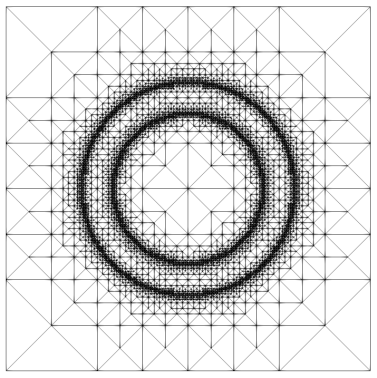
Figure 1: The solution (5.2) at times $t=0$ and $t=\frac{1}{2}$, as well as the adaptive bulk mesh $\mathcal{T}^{M}$.

In Table 1 we display the errors

$$\|\Gamma^{h}-\Gamma\|_{L^{\infty}}=\max_{m=1,\ldots,M}\max_{k=1,\ldots,K}\operatorname{dist}(\vec{q}^{m}_{k},\Gamma(t_{m}))$$

and

$$\|U^{h}-u\|_{L^{\infty}}=\max_{m=1,\ldots,M}\|U^{m}-I^{m}u(\cdot,t_{m})\|_{L^{\infty}(\Omega)},$$

where $I^{m}:C^{0}(\overline{\Omega})\to S^{m}$ denotes the standard interpolation operator. We also let $K_{\Omega}^{m}$ denote the number of degrees of freedom of $S^{m}$, and define $h^{m}_{\Gamma}=\max_{j=1,\ldots,J}\operatorname{diam}(\sigma^{m}_{j})$. As a comparison, we show the same error computations for the linear scheme (3.1) in Table 2. As expected, we observe true volume preservation for the scheme (3.7) in Table 1, up to solver tolerance, while the relative volume loss in Table 2 decreases as $\Delta t$ becomes smaller. Surprisingly, the two error quantities $\|\Gamma^{h}-\Gamma\|_{L^{\infty}}$ and $\|U^{h}-u\|_{L^{\infty}}$ are generally lower in Table 2 compared to Table 1, although the difference becomes smaller with smaller discretization parameters. For completeness, we also present the errors for the same convergence experiment for the two schemes (3.7)^h and (3.1)^h with numerical integration, see Tables 3 and 4.

$h_{f}$	$h^{M}_{\Gamma}$	$\|U^{h}-u\|_{L^{\infty}}$	$\|\Gamma^{h}-\Gamma\|_{L^{\infty}}$	$K^{M}_{\Omega}$	$K$	$|v_{\Delta}^{M}|$
6.2500e-02	1.1400e-01	1.5609e-01	3.4036e-02	2925	256	$<10^{-10}$
3.1250e-02	5.7282e-02	4.5306e-02	1.7416e-02	5101	512	$<10^{-10}$
1.5625e-02	2.8714e-02	1.4406e-02	8.9079e-03	9785	1024	$<10^{-10}$
7.8125e-03	1.4375e-02	5.0773e-03	4.6020e-03	21557	2048	$<10^{-10}$
3.9062e-03	7.1929e-03	2.8734e-03	2.1860e-03	96781	4096	$<10^{-10}$

Table 1: Convergence test for (5.2) over the time interval $[0,\frac{1}{2}]$ for the scheme (3.7).

$h_{f}$	$h^{M}_{\Gamma}$	$\|U^{h}-u\|_{L^{\infty}}$	$\|\Gamma^{h}-\Gamma\|_{L^{\infty}}$	$K^{M}_{\Omega}$	$K$	$|v_{\Delta}^{M}|$
6.2500e-02	1.1497e-01	1.4990e-01	5.1377e-03	2869	256	1.2e-02
3.1250e-02	5.7408e-02	4.3367e-02	7.7591e-03	5097	512	3.2e-03
1.5625e-02	2.8730e-02	1.3917e-02	6.4656e-03	9857	1024	8.3e-04
7.8125e-03	1.4377e-02	4.9546e-03	3.9948e-03	21593	2048	2.1e-04
3.9062e-03	7.1932e-03	2.7345e-03	2.0351e-03	96969	4096	5.1e-05

Table 2: Convergence test for (5.2) over the time interval $[0,\frac{1}{2}]$ for the scheme (3.1).

$h_{f}$	$h^{M}_{\Gamma}$	$\|U^{h}-u\|_{L^{\infty}}$	$\|\Gamma^{h}-\Gamma\|_{L^{\infty}}$	$K^{M}_{\Omega}$	$K$	$|v_{\Delta}^{M}|$
6.2500e-02	1.1433e-01	1.6079e-01	2.4789e-02	2941	256	$<10^{-10}$
3.1250e-02	5.7357e-02	4.9133e-02	1.3107e-02	5077	512	$<10^{-10}$
1.5625e-02	2.8733e-02	1.6422e-02	6.8358e-03	9865	1024	$<10^{-10}$
7.8125e-03	1.4380e-02	6.1040e-03	3.5755e-03	21605	2048	$<10^{-10}$
3.9062e-03	7.1941e-03	2.6860e-03	1.6743e-03	96893	4096	$<10^{-10}$

Table 3: Convergence test for (5.2) over the time interval $[0,\frac{1}{2}]$ for the scheme (3.7)^h.

$h_{f}$	$h^{M}_{\Gamma}$	$\|U^{h}-u\|_{L^{\infty}}$	$\|\Gamma^{h}-\Gamma\|_{L^{\infty}}$	$K^{M}_{\Omega}$	$K$	$|v_{\Delta}^{M}|$
6.2500e-02	1.1530e-01	1.6291e-01	1.3785e-02	2881	256	1.2e-02
3.1250e-02	5.7482e-02	4.7307e-02	4.5358e-03	5185	512	3.2e-03
1.5625e-02	2.8749e-02	1.5926e-02	4.4224e-03	9757	1024	8.2e-04
7.8125e-03	1.4382e-02	5.9809e-03	2.9693e-03	21501	2048	2.1e-04
3.9062e-03	7.1943e-03	2.5431e-03	1.5237e-03	96997	4096	5.1e-05

Table 4: Convergence test for (5.2) over the time interval $[0,\frac{1}{2}]$ for the scheme (3.1)^h.

We also perform a convergence experiment for the true solution (5.2) for $d=3$. To this end, we choose the initial radii $r_{1}(0)=2.5$, $r_{2}(0)=3$ and the time interval $[0,T]$ with $T=0.1$, so that $r_{1}(T)\approx 2.15$ and $r_{2}(T)\approx 2.77$. Moreover, for $i=0\to 3$, we set $N_{f}=2^{5+i}$, $N_{c}=4^{i}$, $\frac{1}{2}K=\widehat{K}(i)$, where $(\widehat{K}(0),\widehat{K}(1),\widehat{K}(2),\widehat{K}(3))=(770,3074,12290,49154)$, and $\tau=4^{3-i}\times 10^{-3}$. The errors $\|U^{h}-u\|_{L^{\infty}}$ and $\|\Gamma^{h}-\Gamma\|_{L^{\infty}}$ for the four schemes (3.7), (3.7)^(h) (3.1) and (3.1)^(h) on the interval $[0,T]$ with $T=0.1$ are displayed in Tables 5, 6, 7 and 8.

$h_{f}$	$h^{M}_{\Gamma}$	$\|U^{h}-u\|_{L^{\infty}}$	$\|\Gamma^{h}-\Gamma\|_{L^{\infty}}$	$K^{M}_{\Omega}$	$K$	$|v_{\Delta}^{M}|$
2.5000e-01	5.6320e-01	7.3514e-01	1.3667e-01	10831	1540	$<10^{-10}$
1.2500e-01	2.8759e-01	2.5135e-01	4.6999e-02	46311	6148	$<10^{-10}$
6.2500e-02	1.4473e-01	9.1052e-02	1.9356e-02	188389	24580	$<10^{-10}$
3.1250e-02	7.2527e-02	3.5851e-02	8.7870e-03	956293	98308	$<10^{-10}$

Table 5: Convergence test for (5.2) over the time interval $[0,0.1]$ for the scheme (3.7).

$h_{f}$	$h^{M}_{\Gamma}$	$\|U^{h}-u\|_{L^{\infty}}$	$\|\Gamma^{h}-\Gamma\|_{L^{\infty}}$	$K^{M}_{\Omega}$	$K$	$|v_{\Delta}^{M}|$
2.5000e-01	5.6594e-01	8.9355e-01	1.3062e-01	10879	1540	$<10^{-10}$
1.2500e-01	2.8815e-01	3.1381e-01	4.3354e-02	46335	6148	$<10^{-10}$
6.2500e-02	1.4484e-01	1.2228e-01	1.7321e-02	188725	24580	$<10^{-10}$
3.1250e-02	7.2548e-02	5.7925e-02	7.6589e-03	970477	98308	$<10^{-10}$

Table 6: Convergence test for (5.2) over the time interval $[0,0.1]$ for the scheme (3.7)^h.

$h_{f}$	$h^{M}_{\Gamma}$	$\|U^{h}-u\|_{L^{\infty}}$	$\|\Gamma^{h}-\Gamma\|_{L^{\infty}}$	$K^{M}_{\Omega}$	$K$	$|v_{\Delta}^{M}|$
2.5000e-01	5.7042e-01	6.5892e-01	6.2158e-02	10879	1540	2.3e-02
1.2500e-01	2.8847e-01	2.3273e-01	3.0705e-02	46375	6148	6.2e-03
6.2500e-02	1.4485e-01	8.6575e-02	1.5551e-02	188725	24580	1.5e-03
3.1250e-02	7.2548e-02	3.4759e-02	7.8760e-03	956293	98308	3.6e-04

Table 7: Convergence test for (5.2) over the time interval $[0,0.1]$ for the scheme (3.1).

$h_{f}$	$h^{M}_{\Gamma}$	$\|U^{h}-u\|_{L^{\infty}}$	$\|\Gamma^{h}-\Gamma\|_{L^{\infty}}$	$K^{M}_{\Omega}$	$K$	$|v_{\Delta}^{M}|$
2.5000e-01	5.7401e-01	7.8420e-01	6.5619e-02	10879	1540	2.2e-02
1.2500e-01	2.8908e-01	2.9887e-01	2.7440e-02	46423	6148	6.0e-03
6.2500e-02	1.4497e-01	1.1943e-01	1.3544e-02	188965	24580	1.5e-03
3.1250e-02	7.2572e-02	5.7009e-02	6.8226e-03	956821	98308	3.6e-04

Table 8: Convergence test for (5.2) over the time interval $[0,0.1]$ for the scheme (3.1)^h.

Similarly to the convergence experiments in 2d, we note that for the schemes (3.1)^(h) the relative volume loss converges to zero as the discretization parameters get smaller, while the schemes (3.7)^(h) preserve the volume exactly in every case. The error quantities $\|U^{h}-u\|_{L^{\infty}}$ and $\|\Gamma^{h}-\Gamma\|_{L^{\infty}}$ behave very similarly for all four schemes.

5.2 Simulations in 2d

In this subsection we consider some numerical experiments for the case $d=2$. In the first computation, we numerically confirm the well-known result shown in [31], which says that the Mullins–Sekerka flow (1.1) does not preserve convexity. To this end, we choose for $\Gamma(0)$ an elongated cigar shape of total dimension $7\times 1$. The discretization parameters for the computation are $N_{f}=128$, $N_{c}=16$, $\Delta t=10^{-3}$, $T=2$ and $K=256$, and the results are shown in Figure 2. We observe that during the evolution the interface becomes nonconvex, before reaching a circular steady state. As expected, the enclosed volume is preserved during the evolution. This is not the case when using the scheme (3.1), as can be seen from Figure 3, where for completeness we show the same simulation for this alternative finite element approximation.

Figure 2: $\Gamma^{m}$ at times $t=0,0.1,\ldots,1,T=2$ for the scheme (3.7). We also show a plot of the discrete energy $|\Gamma^{m}|$ and of the relative volume loss $v_{\Delta}^{m}$ over time.

Figure 3: $\Gamma^{m}$ at times $t=0,0.1,\ldots,1,T=2$ for the scheme (3.1). We also show a plot of the discrete energy $|\Gamma^{m}|$ and of the relative volume loss $v_{\Delta}^{m}$ over time.

Our second simulation is for an anisotropic surface energy. Here we make use of the fact that anisotropies of the form (4.2) can be used to approximate crystalline surface energies, where the isoperimetric minimizers (the so-called Wulff shapes) exhibit flat parts and sharp corners. In particular, we choose the density

$$\gamma_{0}(p)=\tfrac{1}{4}\sum_{\ell=1}^{4}\sqrt{[(R(\tfrac{\pi}{4})^{\ell}]^{T}D(\delta)(R(\tfrac{\pi}{4}))^{\ell}p\cdot p},\quad\delta=10^{-4},$$ (5.5)

where $R(\theta)=\binom{\phantom{-}\cos\theta\ \sin\theta}{-\sin\theta\ \cos\theta}$ and $D(\delta)=\operatorname{diag}(1,\delta^{2})$. Then, inspired by the initial curve from [2, Fig. 0], see also [24, Fig. 7], we perform a computation for our scheme (4.6). We observe that all the facets of the initial data are aligned with the Wulff shape of (5.5) with $\delta=0$, i.e.  regular octagon. For the computations shown in Figure 4 we employed the discretization parameters $N_{f}=256$, $N_{c}=32$, $K=512$ and $\Delta t=10^{-3}$. We note that during the evolution all the facets remain aligned with the facets of the Wulff shape. Some facets grow at the expense of others, leading to some facets vanishing completely. Eventually a scaled Wulff shape is approached as a steady state of the flow. As a comparison, we also show the evolution for the isotropic case for the same initial data, in Figure 5. Here the nonconvex initial data soon evolves to a convex curve, which then converges towards a circle.

Figure 4: $\Gamma^{m}$ at times $t=0,0.1,\ldots,1$, and at time $t=T=3$, for the scheme (4.6). We also show a plot of the discrete energy $|\Gamma^{m}|_{\gamma}$ over time.

Figure 5: $\Gamma^{m}$ at times $t=0,0.1,\ldots,1$, and at time $t=T=3$, for the scheme (3.7). We also show a plot of the discrete energy $|\Gamma^{m}|$ over time.

5.3 Simulations in 3d

We end this section with some numerical simulations for the case $d=3$. All the initial data will always be chosen symmetric with respect to the origin. First we look at the 3d analogue of the experiment in Figure 2, that is we start with an initial interface in the shape of a rounded cylinder with total dimensions $7\times 1\times 1$. The discretization parameters for this computation are $N_{f}=128$, $N_{c}=16$, $\tau=10^{-3}$, $T=2$ and $K=1154$.

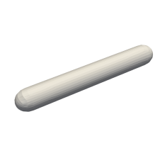
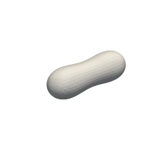
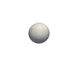
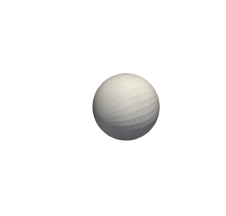
Figure 6: $\Gamma^{m}$ at times $t=0,0.1,0.2,0.5,2$. Below we show a plot of the discrete energy $|\Gamma^{m}|$ and of the relative volume loss $v_{\Delta}^{m}$ over time.

We observe that the initially convex interface loses its convexity during the evolution, which numerically confirms that such evolutions also exist in the case $d=3$. Recall that the corresponding result for $d=2$ has been shown in [31]. For the numerical simulation in Figure 6 we also note that the discrete energy is monotonically decreasing, while the enclosed volume is maintained up to the chosen solver tolerance.

In a second experiment where an initially convex interface loses its convexity, we start the evolution with a rounded cylinder of total dimension $6\times 6\times 1$. We see from the evolution in Figure 7 that the moving interface becomes nonconvex, before it approaches the shape of a sphere. The discretization parameters for this computation are $N_{f}=128$, $N_{c}=16$, $\tau=10^{-3}$, $T=2$ and $K=1538$.

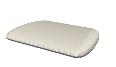
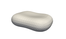
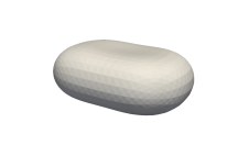
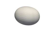
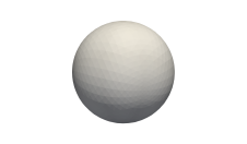
Figure 7: $\Gamma^{m}$ at times $t=0,0.1,0.2,0.5,2$. Below we show a plot of the discrete energy $|\Gamma^{m}|$ and of the relative volume loss $v_{\Delta}^{m}$ over time.

We also present two simulations for an anisotropic surface energy. In the first one, we repeat the simulation in Figure 6, with the same discretization parameters as before, but now for the anisotropy

$$\gamma(\vec{p})=\sum_{i=1}^{3}\left[\delta^{2}|\vec{p}|^{2}+p_{i}^{2}(1-\delta^{2})\right]^{\frac{1}{2}},\quad\delta=0.1,$$

which approximates the $\ell^{1}$–norm of $\vec{p}$. For the computation in Figure 8 it can be observed that, as in the isotropic case, the interface loses its convexity. Eventually it settles down to an approximation of the Wulff shape, which here is a smoothed cube.

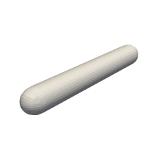
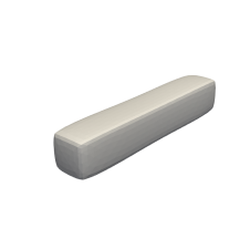
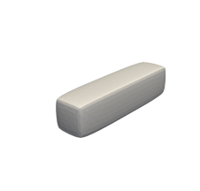
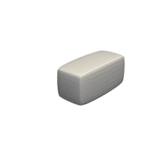
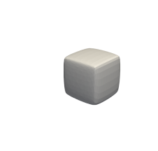
Figure 8: $\Gamma^{m}$ at times $t=0,0.05,0.1,0.2,2$. Below we show a plot of the discrete energy $|\Gamma^{m}|_{\gamma}$ and of the relative volume loss $v_{\Delta}^{m}$ over time.

In the final simulation we use an anisotropic energy of the form (4.2) with $r>1$, so that the iteration (4.10) also has to account for the nonlinearity in the approximation of the anisotropy in (4.6). In particular, we choose

$$\gamma(\vec{p})=\left(\sum_{i=1}^{3}\left[\delta^{2}|\vec{p}|^{2}+p_{i}^{2}(1-\delta^{2})\right]^{\frac{r}{2}}\right)^{\frac{1}{r}},\quad\delta=0.1,\ r=9,$$

in order to model an anisotropy with an octahedral Wulff shape, see e.g. [6, Figs. 4, 15]. For the experiment in Figure 9 we start from the same rounded cylinder of total dimension $6\times 6\times 1$ from Figure 7, and also use the discretization parameters from the earlier simulation. During the interesting evolution the moving interface approaches the Wulff shape, and decreases its anisotropic surface energy as it does so. As expected, the numerical approximation conserves the enclosed volume exactly.

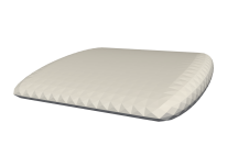
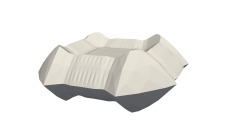
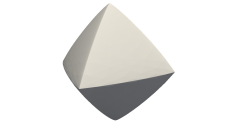
Figure 9: $\Gamma^{m}$ at times $t=0,0.1,0.2,0.5,2$. Below we show a plot of the discrete energy $|\Gamma^{m}|$ and of the relative volume loss $v_{\Delta}^{m}$ over time.

References

[1]N. D. Alikakos, P. W. Bates, and X. Chen, Convergence of the
Cahn–Hilliard equation to the Hele–Shaw model, Arch. Rational
Mech. Anal., 128 (1994), pp. 165–205.
[2]F. Almgren and J. E. Taylor, Flat flow is motion by crystalline
curvature for curves with crystalline energies, J. Differential Geom., 42
(1995), pp. 1–22.
[3]W. Bao and Q. Zhao, A structure-preserving parametric finite element
method for surface diffusion, SIAM J. Numer. Anal., 59 (2021),
pp. 2775–2799.
[4]J. W. Barrett, H. Garcke, and R. Nürnberg, Numerical approximation
of anisotropic geometric evolution equations in the plane, IMA J. Numer.
Anal., 28 (2008), pp. 292–330.
[5], On the parametric
finite element approximation of evolving hypersurfaces in ,
J. Comput. Phys., 227 (2008), pp. 4281–4307.
[6], A variational
formulation of anisotropic geometric evolution equations in higher
dimensions, Numer. Math., 109 (2008), pp. 1–44.
[7], On stable parametric
finite element methods for the Stefan problem and the Mullins–Sekerka
problem with applications to dendritic growth, J. Comput. Phys., 229 (2010),
pp. 6270–6299.
[8], Eliminating spurious
velocities with a stable approximation of viscous incompressible two-phase
Stokes flow, Comput. Methods Appl. Mech. Engrg., 267 (2013), pp. 511–530.
[9], On the stable
discretization of strongly anisotropic phase field models with applications
to crystal growth, ZAMM Z. Angew. Math. Mech., 93 (2013), pp. 719–732.
[10], Stable phase field
approximations of anisotropic solidification, IMA J. Numer. Anal., 34
(2014), pp. 1289–1327.
[11], A stable parametric
finite element discretization of two-phase Navier–Stokes flow, J. Sci.
Comp., 63 (2015), pp. 78–117.
[12], On the stable
numerical approximation of two-phase flow with insoluble surfactant, ESAIM
Math. Model. Numer. Anal., 49 (2015), pp. 421–458.
[13], Parametric finite
element approximations of curvature driven interface evolutions, in Handb.
Numer. Anal., A. Bonito and R. H. Nochetto, eds., vol. 21, Elsevier,
Amsterdam, 2020, pp. 275–423.
[14]P. W. Bates, X. Chen, and X. Deng, A numerical scheme for the two
phase Mullins–Sekerka problem, Electron. J. Differential Equations,
1995 (1995), pp. 1–28.
[15]G. Bellettini, M. Novaga, and M. Paolini, Facet-breaking for
three-dimensional crystals evolving by mean curvature, Interfaces Free
Bound., 1 (1999), pp. 39–55.
[16]J. W. Cahn and J. E. Hilliard, Free energy of a non-uniform system.
I. Interfacial free energy, J. Chem. Phys., 28 (1958), pp. 258–267.
[17]J. W. Cahn and J. E. Taylor, Surface motion by surface diffusion,
Acta Metall. Mater., 42 (1994), pp. 1045–1063.
[18]S. Chen, B. Merriman, S. Osher, and P. Smereka, A simple level set
method for solving Stefan problems, J. Comput. Phys., 135 (1997),
pp. 8–29.
[19]X. Chen, The Hele-Shaw problem and area-preserving
curve-shortening motions, Arch. Rational Mech. Anal., 123 (1993),
pp. 117–151.
[20]X. Chen, J. Hong, and F. Yi, Existence, uniqueness, and regularity
of classical solutions of the Mullins–Sekerka problem, Comm. Partial
Differential Equations, 21 (1996), pp. 1705–1727.
[21]P. G. Ciarlet, The Finite Element Method for Elliptic Problems,
North-Holland Publishing Co., Amsterdam, 1978.
Studies in Mathematics and its Applications, Vol. 4.
[22]T. A. Davis, Algorithm 832: UMFPACK V4.3—an
unsymmetric-pattern multifrontal method, ACM Trans. Math. Software, 30
(2004), pp. 196–199.
[23]K. Deckelnick, G. Dziuk, and C. M. Elliott, Computation of geometric
partial differential equations and mean curvature flow, Acta Numer., 14
(2005), pp. 139–232.
[24]K. Deckelnick and R. Nürnberg, A novel finite element
approximation of anisotropic curve shortening flow.
arXiv:2110.04605, 2021.
[25]G. Dziuk, An algorithm for evolutionary surfaces, Numer. Math., 58
(1991), pp. 603–611.
[26]J. Escher and G. Simonett, Classical solutions for Hele–Shaw
models with surface tension, Adv. Differential Equations, 2 (1997),
pp. 619–642.
[27]X. Feng and A. Prohl, Analysis of a fully discrete finite element
method for the phase field model and approximation of its sharp interface
limits, Math. Comp., 73 (2004), pp. 541–567.
[28], Error analysis of a
mixed finite element method for the Cahn–Hilliard equation, Numer.
Math., 99 (2004), pp. 47–84.
[29]Y. Giga, Surface evolution equations, vol. 99 of Monographs in
Mathematics, Birkhäuser, Basel, 2006.
[30]W. Jiang and B. Li, A perimeter-decreasing and area-conserving
algorithm for surface diffusion flow of curves, J. Comput. Phys., 443
(2021), pp. Paper No. 110531, 11.
[31]U. F. Mayer, Two-sided Mullins–Sekerka flow does not preserve
convexity, in Proceedings of the Third Mississippi State Conference
on Difference Equations and Computational Simulations (Mississippi
State, MS, 1997), vol. 1 of Electron. J. Differ. Equ. Conf., San Marcos,
TX, 1998, Southwest Texas State Univ., pp. 171–179.
[32], A numerical scheme
for moving boundary problems that are gradient flows for the area
functional, European J. Appl. Math., 11 (2000), pp. 61–80.
[33]W. W. Mullins and R. F. Sekerka, Morphological stability of a
particle growing by diffusion or heat flow, J. Appl. Phys., 34 (1963),
pp. 323–329.
[34]A. Schmidt and K. G. Siebert, Design of Adaptive Finite Element
Software: The Finite Element Toolbox ALBERTA, vol. 42 of Lecture Notes in
Computational Science and Engineering, Springer-Verlag, Berlin, 2005.
[35]J. E. Taylor and J. W. Cahn, Linking anisotropic sharp and diffuse
surface motion laws via gradient flows, J. Statist. Phys., 77 (1994),
pp. 183–197.
[36]J. E. Taylor, J. W. Cahn, and C. A. Handwerker, Geometric models of
crystal growth, Acta Metall. Mater., 40 (1992), pp. 1443–1474.
[37]J. Zhu, X. Chen, and T. Y. Hou, An efficient boundary integral
method for the Mullins–Sekerka problem, J. Comput. Phys., 127 (1996),
pp. 246–267.