A Fourier transform for all generalized functions

Abstract.

Using the existence of infinite numbers $k$ in the non-Archimedean ring of Robinson-Colombeau, we define the hyperfinite Fourier transform (HFT) by considering integration extended to $[-k,k]^{n}$ instead of $(-\infty,\infty)^{n}$. In order to realize this idea, the space of generalized functions we consider is that of generalized smooth functions (GSF), an extension of classical distribution theory sharing many nonlinear properties with ordinary smooth functions, like the closure with respect to composition, a good integration theory, and several classical theorems of calculus. Even if the final transform depends on $k$, we obtain a new notion that applies to all GSF, in particular to all Schwartz’s distributions and to all Colombeau generalized functions defined in $[-k,k]^{n}$, without growth restrictions. We prove that this FT generalizes several classical properties of the ordinary FT, and in this way we also overcome the difficulties of FT in Colombeau’s settings. Differences in some formulas, such as in the transform of derivatives, reveal to be meaningful since allow to obtain also non-tempered global solutions of differential equations.

1. Introduction: extending the domain of the Fourier transform

Fourier transform (FT) and generalized functions (GF) are naturally interwoven, since the former naturally leads to suitable spaces of the latter. This already occurs even in trivial cases, such as transforming a simple sound wave $f(t)=A\sin(2\pi\omega_{0}t)$, whose spectrum must be, in some way, concentrated at the frequencies $\pm\omega_{0}$. Even the link between constants and delta-like functions was already conceived by Fourier (see e.g. [42]). Although different theories of generalized functions arise for different motivations, from distribution theory of Sobolev, Schwartz [56, 59] up to Hairer’s regularity structures [32], almost all these theories are usually augmented with a corresponding calculus of FT, which can be applied to an appropriate subspace of generalized functions. Since the beginning of distribution theory, it was hence natural to try to extend the domain of the FT with less or even with no growth restrictions imposed. In fact, e.g., as a consequence of these restrictions, the only solution of the trivial ODE $y^{\prime}=y$ we can achieve using tempered distributions is the trivial one. We can hence cite in [21, 22] the definition of the FT as the limit of a sequence of functions integrated on a finite domain, or [67] for a two-sided Laplace transform defined on a space larger than that of tempered distributions, and similarly in [3] for the directional short-time Fourier transform of exponential-type distributions. In the same direction we can inscribe the works [2, 9, 15, 37, 52, 61, 58, 18, 19] on ultradistributions, hyperfunctions and thick distributions.

On the other hand, problems originating from physics, such as singularities and point-source fields, also suggest us to consider alternative modeling, ranging from non-smooth functions as test functions in the theory of distributions (see e.g. [65] and references therein) to non-Archimedean analysis (i.e. mathematical analysis over a ring extending the real field and containing infinitesimal and/or infinite numbers, see [31, 20]). In the interplay between mathematics and physics, it is well-known that heuristically manipulating non-linear pointwise equalities such as $H^{2}=H$ ($H$ being the Heaviside function) can easily lead to contradictions (see e.g. [8, 31]). This can make particularly difficult to realize the strategy of [44], where the authors search for a metaplectic representation from symplectic maps to symplectic relations. According to A. Weinstein (personal communication, May 2019), this would require an algebra of generalized functions extending the usual algebra of smooth functions and a FT acting on them with the usual inversion formula and transforming the Dirac delta into $1$. As we will see more diffusely in the following sections, this is not possible in the classical approach to Colombeau’s algebra, see [11, 13, 48, 35]. We will only arrive at a partial solution of this problem where equalities are replaced by infinitely closed relations or by limits, see Cor. 67 and Thm. 61, Cor.64.

To overcome this type of problems, we are going to use the category of generalized smooth functions (GSF), see [25, 26, 43, 24, 27]. This theory seems to be a good candidate, since it is an extension of classical distribution theory which allows to model nonlinear singular problems, while at the same time sharing many nonlinear properties with ordinary smooth functions, like the closure with respect to composition (thereby, they form an algebra extending the algebra of smooth functions with pointwise product) and several non trivial classical theorems of the calculus. One could describe GSF as a methodological restoration of Cauchy-Dirac’s original conception of generalized function, see [16, 41, 39]. In essence, the idea of Cauchy and Dirac (but also of Poisson, Kirchhoff, Helmholtz, Kelvin and Heaviside) was to view generalized functions as suitable types of smooth set-theoretical maps obtained from ordinary smooth maps depending on suitable infinitesimal or infinite parameters. For example, the density of a Cauchy-Lorentz distribution with an infinitesimal scale parameter was used by Cauchy to obtain classical properties which nowadays are attributed to the Dirac delta, cf. [39].

The basic idea to define a very general FT in this setting is the following: Since GSF form a non-Archimedean framework, we can consider a positive infinite generalized number $k$ (i.e. $k>r$ for all $r\in\mathbb{R}_{>0}$) and define the FT with the usual formula, but integrating over the $n$-dimensional interval $[-k,k]^{n}$. Although $k$ is an infinite number (hence, $[-k,k]^{n}\supseteq\mathbb{R}^{n}$), this interval behaves like a compact set for GSF, so that, e.g., on these domains we always have an extreme value theorem and integrals always exist. Clearly, this leads to a FT, called hyperfinite FT, that depends on the parameter $k$, but, on the other hand, where we can transform all the GSF defined on this interval and these include all tempered Schwartz distributions, all tempered Colombeau GF, but also a large class of non-tempered GF, such as the exponential functions, or non-linear examples like $\delta^{a}\circ\delta^{b}$, $\delta^{a}\circ H^{b}$, $a$, $b\in\mathbb{N}$, etc. Not all the properties of the classical FT remain unchanged for this more general transform, but the final formalism still retains the useful properties of the FT in dealing with differential equations. Even more, the new formula for the transform of derivatives leads to discover also exponential solutions of the aforementioned ODE $y^{\prime}=y$. Since [14] proves that ultradistributions and periodic hyperfunctions can be embedded in Colombeau type algebra, this give strong hints to conjecture that the hyperfinite FT is very general, and it justifies the title of this article.

The structure of the paper is as follows. We start with an introduction into the setting of GSF and give basic notions concerning GSF and their calculus that are needed for a first study of the hyperfinite FT (Sec. 2). We then define the hyperfinite FT in Sec. 4 and the convolution of compactly supported GSF in Sec. 3. In Sec. 6, we show how the elementary properties of FT change for the hyperfinite FT. In Sec. 7 and Sec. 8, we respectively prove the inversion theorem and that the embedding of a very large class of Sobolev-Schwartz tempered distributions preserves their FT, i.e. that the hyperfinite FT commutes with the embedding of Schwartz functions and tempered distributions. In this section, we also recall the problems of FT in the Colombeau’s setting and how we overcome them. Finally, in Sec. 9 we give several examples which underscore the new possibility to transform any generalized functions. Thanks to the developed formalism, which stresses the similarities with ordinary smooth functions, frequently the proofs we are going to present are very simple and similar to those for smooth functions, but replacing the real field $\mathbb{R}$ with the non-Archimedean ring of Robinson-Colombeau $\mathchoice{{\vphantom{\mathbb{R}}}^{\scalebox{0.6}{$\rho$}}}{{\vphantom{\mathbb{R}}}^{\scalebox{0.56}{$\rho$}}}{{\vphantom{\mathbb{R}}}^{\scalebox{0.47}{$\rho$}}}{{\vphantom{\mathbb{R}}}^{\scalebox{0.35}{$\rho$}}}\widetilde{\mathbb{R}}$.

The paper is self-contained, in the sense that it contains all the statements required for the proofs we are going to present. If proofs of preliminaries are omitted, we clearly give references to where they can be found. Therefore, to understand this paper, only a basic knowledge of distribution theory is needed.

2. Basic notions

2.1. The new ring of scalars

In this work, $I$ denotes the interval $(0,1]\subseteq\mathbb{R}$ and we will always use the variable $\varepsilon$ for elements of $I$; we also denote $\varepsilon$-dependent nets $x\in\mathbb{R}^{I}$ simply by $(x_{\varepsilon})$. By $\mathbb{N}$ we denote the set of natural numbers, including zero.

We start by defining a new simple non-Archimedean ring of scalars that extends the real field $\mathbb{R}$. The entire theory is constructive to a high degree, e.g. neither ultrafilter nor non-standard method are used. For all the proofs of results in this section, see [24, 25, 27, 26].

Definition 1.

Let $\rho=(\rho_{\varepsilon})\in(0,1]^{I}$ be a net such that $(\rho_{\varepsilon})\to 0$ as $\varepsilon\to 0^{+}$ (in the following, such a net will be called a gauge), then

1. $\mathcal{I}(\rho):=\left\{(\rho_{\varepsilon}^{-a})\mid a\in\mathbb{R}_{>0}\right\}$ is called the asymptotic gauge generated by $\rho$.

2. If $\mathcal{P}(\varepsilon)$ is a property of $\varepsilon\in I$, we use the notation $\forall^{0}\varepsilon:\,\mathcal{P}(\varepsilon)$ to denote $\exists\varepsilon_{0}\in I\,\forall\varepsilon\in(0,\varepsilon_{0}]:\,\mathcal{P}(\varepsilon)$. We can read $\forall^{0}\varepsilon$ as for $\varepsilon$ small.

3. We say that a net $(x_{\varepsilon})\in\mathbb{R}^{I}$ is $\rho$-moderate, and we write $(x_{\varepsilon})\in\mathbb{R}_{\rho}$ if

   $$\exists(J_{\varepsilon})\in\mathcal{I}(\rho):\ x_{\varepsilon}=O(J_{\varepsilon})\text{ as }\varepsilon\to 0^{+},$$

   i.e., if

   $$\exists N\in\mathbb{N}\,\forall^{0}\varepsilon:\ |x_{\varepsilon}|\leq\rho_{\varepsilon}^{-N}.$$

4. Let $(x_{\varepsilon})$, $(y_{\varepsilon})\in\mathbb{R}^{I}$, then we say that $(x_{\varepsilon})\sim_{\rho}(y_{\varepsilon})$ if

   $$\forall(J_{\varepsilon})\in\mathcal{I}(\rho):\ x_{\varepsilon}=y_{\varepsilon}+O(J_{\varepsilon}^{-1})\text{ as }\varepsilon\to 0^{+},$$

   that is if

   $$\forall n\in\mathbb{N}\,\forall^{0}\varepsilon:\ |x_{\varepsilon}-y_{\varepsilon}|\leq\rho_{\varepsilon}^{n}.$$ (2.1)

   This is a congruence relation on the ring $\mathbb{R}_{\rho}$ of moderate nets with respect to pointwise operations, and we can hence define

   $$\mathchoice{{\vphantom{\mathbb{R}}}^{\scalebox{0.6}{$\rho$}}}{{\vphantom{\mathbb{R}}}^{\scalebox{0.56}{$\rho$}}}{{\vphantom{\mathbb{R}}}^{\scalebox{0.47}{$\rho$}}}{{\vphantom{\mathbb{R}}}^{\scalebox{0.35}{$\rho$}}}\widetilde{\mathbb{R}}:=\mathbb{R}_{\rho}/\sim_{\rho},$$

   which we call Robinson-Colombeau ring of generalized numbers. This name is justified by [55, 10]: Indeed, in [55] A. Robinson introduced the notion of moderate and negligible nets depending on an arbitrary fixed infinitesimal $\rho$ (in the framework of nonstandard analysis); independently, J.F. Colombeau, cf. e.g. [10] and references therein, studied the same concepts without using nonstandard analysis, but considering only the particular gauge $\rho_{\varepsilon}=\varepsilon$.

We will also use other directed sets instead of $I$: e.g. $J\subseteq I$ such that $0$ is a closure point of $J$, or $I\times\mathbb{N}$. The reader can easily check that all our constructions can be repeated in these cases. We can also define an order relation on $\mathchoice{{\vphantom{\mathbb{R}}}^{\scalebox{0.6}{$\rho$}}}{{\vphantom{\mathbb{R}}}^{\scalebox{0.56}{$\rho$}}}{{\vphantom{\mathbb{R}}}^{\scalebox{0.47}{$\rho$}}}{{\vphantom{\mathbb{R}}}^{\scalebox{0.35}{$\rho$}}}\widetilde{\mathbb{R}}$ by saying that $[x_{\varepsilon}]\leq[y_{\varepsilon}]$ if there exists $(z_{\varepsilon})\in\mathbb{R}^{I}$ such that $(z_{\varepsilon})\sim_{\rho}0$ (we then say that $(z_{\varepsilon})$ is $\rho$-negligible) and $x_{\varepsilon}\leq y_{\varepsilon}+z_{\varepsilon}$ for $\varepsilon$ small. Equivalently, we have that $x\leq y$ if and only if there exist representatives $[x_{\varepsilon}]=x$ and $[y_{\varepsilon}]=y$ such that $x_{\varepsilon}\leq y_{\varepsilon}$ for all $\varepsilon$. Although the order $\leq$ is not total, we still have the possibility to define the infimum $[x_{\varepsilon}]\wedge[y_{\varepsilon}]:=[\min(x_{\varepsilon},y_{\varepsilon})]$, the supremum $[x_{\varepsilon}]\vee[y_{\varepsilon}]:=\left[\max(x_{\varepsilon},y_{\varepsilon})\right]$ of a finite number of generalized numbers. See [47] for a complete study of supremum and infimum in $\mathchoice{{\vphantom{\mathbb{R}}}^{\scalebox{0.6}{$\rho$}}}{{\vphantom{\mathbb{R}}}^{\scalebox{0.56}{$\rho$}}}{{\vphantom{\mathbb{R}}}^{\scalebox{0.47}{$\rho$}}}{{\vphantom{\mathbb{R}}}^{\scalebox{0.35}{$\rho$}}}\widetilde{\mathbb{R}}$. Henceforth, we will also use the customary notation $\mathchoice{{\vphantom{\mathbb{R}}}^{\scalebox{0.6}{$\rho$}}}{{\vphantom{\mathbb{R}}}^{\scalebox{0.56}{$\rho$}}}{{\vphantom{\mathbb{R}}}^{\scalebox{0.47}{$\rho$}}}{{\vphantom{\mathbb{R}}}^{\scalebox{0.35}{$\rho$}}}\widetilde{\mathbb{R}}^{*}$ for the set of invertible generalized numbers, and we write $x<y$ to say that $x\leq y$ and $x-y\in\mathchoice{{\vphantom{\mathbb{R}}}^{\scalebox{0.6}{$\rho$}}}{{\vphantom{\mathbb{R}}}^{\scalebox{0.56}{$\rho$}}}{{\vphantom{\mathbb{R}}}^{\scalebox{0.47}{$\rho$}}}{{\vphantom{\mathbb{R}}}^{\scalebox{0.35}{$\rho$}}}\widetilde{\mathbb{R}}^{*}$. Our notations for intervals are: $[a,b]:=\{x\in\mathchoice{{\vphantom{\mathbb{R}}}^{\scalebox{0.6}{$\rho$}}}{{\vphantom{\mathbb{R}}}^{\scalebox{0.56}{$\rho$}}}{{\vphantom{\mathbb{R}}}^{\scalebox{0.47}{$\rho$}}}{{\vphantom{\mathbb{R}}}^{\scalebox{0.35}{$\rho$}}}\widetilde{\mathbb{R}}\mid a\leq x\leq b\}$, $[a,b]_{\mathbb{R}}:=[a,b]\cap\mathbb{R}$, and analogously for segments $[x,y]:=\left\{x+r\cdot(y-x)\mid r\in[0,1]\right\}\subseteq\mathchoice{{\vphantom{\mathbb{R}}}^{\scalebox{0.6}{$\rho$}}}{{\vphantom{\mathbb{R}}}^{\scalebox{0.56}{$\rho$}}}{{\vphantom{\mathbb{R}}}^{\scalebox{0.47}{$\rho$}}}{{\vphantom{\mathbb{R}}}^{\scalebox{0.35}{$\rho$}}}\widetilde{\mathbb{R}}^{n}$ and $[x,y]_{\mathbb{R}^{n}}=[x,y]\cap\mathbb{R}^{n}$. We also set $\mathbb{C}_{\rho}:=\mathbb{R}_{\rho}+i\cdot\mathbb{R}_{\rho}$ and $\mathchoice{{\vphantom{\mathbb{C}}}^{\scalebox{0.6}{$\rho$}}}{{\vphantom{\mathbb{C}}}^{\scalebox{0.56}{$\rho$}}}{{\vphantom{\mathbb{C}}}^{\scalebox{0.47}{$\rho$}}}{{\vphantom{\mathbb{C}}}^{\scalebox{0.35}{$\rho$}}}\widetilde{\mathbb{C}}:=\mathchoice{{\vphantom{\mathbb{R}}}^{\scalebox{0.6}{$\rho$}}}{{\vphantom{\mathbb{R}}}^{\scalebox{0.56}{$\rho$}}}{{\vphantom{\mathbb{R}}}^{\scalebox{0.47}{$\rho$}}}{{\vphantom{\mathbb{R}}}^{\scalebox{0.35}{$\rho$}}}\widetilde{\mathbb{R}}+i\cdot\mathchoice{{\vphantom{\mathbb{R}}}^{\scalebox{0.6}{$\rho$}}}{{\vphantom{\mathbb{R}}}^{\scalebox{0.56}{$\rho$}}}{{\vphantom{\mathbb{R}}}^{\scalebox{0.47}{$\rho$}}}{{\vphantom{\mathbb{R}}}^{\scalebox{0.35}{$\rho$}}}\widetilde{\mathbb{R}}$, where $i=\sqrt{-1}$. On the $\mathchoice{{\vphantom{\mathbb{R}}}^{\scalebox{0.6}{$\rho$}}}{{\vphantom{\mathbb{R}}}^{\scalebox{0.56}{$\rho$}}}{{\vphantom{\mathbb{R}}}^{\scalebox{0.47}{$\rho$}}}{{\vphantom{\mathbb{R}}}^{\scalebox{0.35}{$\rho$}}}\widetilde{\mathbb{R}}$-module $\mathchoice{{\vphantom{\mathbb{R}}}^{\scalebox{0.6}{$\rho$}}}{{\vphantom{\mathbb{R}}}^{\scalebox{0.56}{$\rho$}}}{{\vphantom{\mathbb{R}}}^{\scalebox{0.47}{$\rho$}}}{{\vphantom{\mathbb{R}}}^{\scalebox{0.35}{$\rho$}}}\widetilde{\mathbb{R}}^{n}$ we can consider the natural extension of the Euclidean norm, i.e. $|[x_{\varepsilon}]|:=[|x_{\varepsilon}|]\in\mathchoice{{\vphantom{\mathbb{R}}}^{\scalebox{0.6}{$\rho$}}}{{\vphantom{\mathbb{R}}}^{\scalebox{0.56}{$\rho$}}}{{\vphantom{\mathbb{R}}}^{\scalebox{0.47}{$\rho$}}}{{\vphantom{\mathbb{R}}}^{\scalebox{0.35}{$\rho$}}}\widetilde{\mathbb{R}}$, where $[x_{\varepsilon}]\in\mathchoice{{\vphantom{\mathbb{R}}}^{\scalebox{0.6}{$\rho$}}}{{\vphantom{\mathbb{R}}}^{\scalebox{0.56}{$\rho$}}}{{\vphantom{\mathbb{R}}}^{\scalebox{0.47}{$\rho$}}}{{\vphantom{\mathbb{R}}}^{\scalebox{0.35}{$\rho$}}}\widetilde{\mathbb{R}}^{n}$.

As in every non-Archimedean ring, we have the following

Definition 2.

Let $x\in\mathchoice{{\vphantom{\mathbb{R}}}^{\scalebox{0.6}{$\rho$}}}{{\vphantom{\mathbb{R}}}^{\scalebox{0.56}{$\rho$}}}{{\vphantom{\mathbb{R}}}^{\scalebox{0.47}{$\rho$}}}{{\vphantom{\mathbb{R}}}^{\scalebox{0.35}{$\rho$}}}\widetilde{\mathbb{R}}^{n}$ be a generalized number, then

1. $x$ is infinitesimal if $|x|\leq r$ for all $r\in\mathbb{R}_{>0}$. If $x=[x_{\varepsilon}]$, this is equivalent to $\lim_{\varepsilon\to 0^{+}}\left|x_{\varepsilon}\right|=0$. We write $x\approx y$ if $x-y$ is infinitesimal.

2. $x$ is finite if $|x|\leq r$ for some $r\in\mathbb{R}_{>0}$.

3. $x$ is infinite if $|x|\geq r$ for all $r\in\mathbb{R}_{>0}$. If $x=[x_{\varepsilon}]$, this is equivalent to $\lim_{\varepsilon\to 0^{+}}\left|x_{\varepsilon}\right|=+\infty$.

For example, setting $\mathchoice{\hbox{\rm d}\rho}{\hbox{\rm d}\rho}{\scalebox{0.75}{$\hbox{\rm d}\rho$}}{\scalebox{0.35}{$\hbox{\rm d}\rho$}}:=[\rho_{\varepsilon}]\in\mathchoice{{\vphantom{\mathbb{R}}}^{\scalebox{0.6}{$\rho$}}}{{\vphantom{\mathbb{R}}}^{\scalebox{0.56}{$\rho$}}}{{\vphantom{\mathbb{R}}}^{\scalebox{0.47}{$\rho$}}}{{\vphantom{\mathbb{R}}}^{\scalebox{0.35}{$\rho$}}}\widetilde{\mathbb{R}}$, we have that $\mathchoice{\hbox{\rm d}\rho}{\hbox{\rm d}\rho}{\scalebox{0.75}{$\hbox{\rm d}\rho$}}{\scalebox{0.35}{$\hbox{\rm d}\rho$}}^{n}\in\mathchoice{{\vphantom{\mathbb{R}}}^{\scalebox{0.6}{$\rho$}}}{{\vphantom{\mathbb{R}}}^{\scalebox{0.56}{$\rho$}}}{{\vphantom{\mathbb{R}}}^{\scalebox{0.47}{$\rho$}}}{{\vphantom{\mathbb{R}}}^{\scalebox{0.35}{$\rho$}}}\widetilde{\mathbb{R}}$, $n\in\mathbb{N}_{>0}$, is an invertible infinitesimal, whose reciprocal is $\mathchoice{\hbox{\rm d}\rho}{\hbox{\rm d}\rho}{\scalebox{0.75}{$\hbox{\rm d}\rho$}}{\scalebox{0.35}{$\hbox{\rm d}\rho$}}^{-n}=[\rho_{\varepsilon}^{-n}]$, which is necessarily a positive infinite number. Of course, in the ring $\mathchoice{{\vphantom{\mathbb{R}}}^{\scalebox{0.6}{$\rho$}}}{{\vphantom{\mathbb{R}}}^{\scalebox{0.56}{$\rho$}}}{{\vphantom{\mathbb{R}}}^{\scalebox{0.47}{$\rho$}}}{{\vphantom{\mathbb{R}}}^{\scalebox{0.35}{$\rho$}}}\widetilde{\mathbb{R}}$ there exist generalized numbers which are not in any of the three classes of Def. 2, like e.g. $x_{\varepsilon}=\frac{1}{\varepsilon}\sin\left(\frac{1}{\varepsilon}\right)$.

Definition 3.

We say that $x$ is a strong infinite number if $|x|\geq\mathchoice{\hbox{\rm d}\rho}{\hbox{\rm d}\rho}{\scalebox{0.75}{$\hbox{\rm d}\rho$}}{\scalebox{0.35}{$\hbox{\rm d}\rho$}}^{-r}$ for some $r\in\mathbb{R}_{>0}$, whereas we say that $x$ is a weak infinite number if $|x|\leq\mathchoice{\hbox{\rm d}\rho}{\hbox{\rm d}\rho}{\scalebox{0.75}{$\hbox{\rm d}\rho$}}{\scalebox{0.35}{$\hbox{\rm d}\rho$}}^{-r}$ for all $r\in\mathbb{R}_{>0}$. For example, $x=-N\log\mathchoice{\hbox{\rm d}\rho}{\hbox{\rm d}\rho}{\scalebox{0.75}{$\hbox{\rm d}\rho$}}{\scalebox{0.35}{$\hbox{\rm d}\rho$}}$, $N\in\mathbb{N},$ is a weak infinite number, whereas if $x_{\varepsilon}=\rho_{\varepsilon}^{-1}$ for $\varepsilon=\frac{1}{k}$, $k\in\mathbb{N}_{>0}$, and $x_{\varepsilon}=-\log\rho_{\varepsilon}$ otherwise, then $x$ is neither a strong nor a weak infinite number.

The following result is useful to deal with positive and invertible generalized numbers. For its proof, see e.g. [31].

Lemma 4.

Let $x\in\mathchoice{{\vphantom{\mathbb{R}}}^{\scalebox{0.6}{$\rho$}}}{{\vphantom{\mathbb{R}}}^{\scalebox{0.56}{$\rho$}}}{{\vphantom{\mathbb{R}}}^{\scalebox{0.47}{$\rho$}}}{{\vphantom{\mathbb{R}}}^{\scalebox{0.35}{$\rho$}}}\widetilde{\mathbb{R}}$. Then the following are equivalent:

1. $x$ is invertible and $x\geq 0$, i.e. $x>0$.

2. For each representative $(x_{\varepsilon})\in\mathbb{R}_{\rho}$ of $x$ we have $\forall^{0}\varepsilon:\ x_{\varepsilon}>0$.

3. For each representative $(x_{\varepsilon})\in\mathbb{R}_{\rho}$ of $x$ we have $\exists m\in\mathbb{N}\,\forall^{0}\varepsilon:\ x_{\varepsilon}>\rho_{\varepsilon}^{m}$.

4. There exists a representative $(x_{\varepsilon})\in\mathbb{R}_{\rho}$ of $x$ such that $\exists m\in\mathbb{N}\,\forall^{0}\varepsilon:\ x_{\varepsilon}>\rho_{\varepsilon}^{m}$.

2.2. Topologies on $\mathchoice{{\vphantom{\mathbb{R}}}^{\scalebox{0.6}{$\rho$}}}{{\vphantom{\mathbb{R}}}^{\scalebox{0.56}{$\rho$}}}{{\vphantom{\mathbb{R}}}^{\scalebox{0.47}{$\rho$}}}{{\vphantom{\mathbb{R}}}^{\scalebox{0.35}{$\rho$}}}\widetilde{\mathbb{R}}^{n}$

As we mentioned above, on the $\mathchoice{{\vphantom{\mathbb{R}}}^{\scalebox{0.6}{$\rho$}}}{{\vphantom{\mathbb{R}}}^{\scalebox{0.56}{$\rho$}}}{{\vphantom{\mathbb{R}}}^{\scalebox{0.47}{$\rho$}}}{{\vphantom{\mathbb{R}}}^{\scalebox{0.35}{$\rho$}}}\widetilde{\mathbb{R}}$-module $\mathchoice{{\vphantom{\mathbb{R}}}^{\scalebox{0.6}{$\rho$}}}{{\vphantom{\mathbb{R}}}^{\scalebox{0.56}{$\rho$}}}{{\vphantom{\mathbb{R}}}^{\scalebox{0.47}{$\rho$}}}{{\vphantom{\mathbb{R}}}^{\scalebox{0.35}{$\rho$}}}\widetilde{\mathbb{R}}^{n}$ we defined $|[x_{\varepsilon}]|:=[|x_{\varepsilon}|]\in\mathchoice{{\vphantom{\mathbb{R}}}^{\scalebox{0.6}{$\rho$}}}{{\vphantom{\mathbb{R}}}^{\scalebox{0.56}{$\rho$}}}{{\vphantom{\mathbb{R}}}^{\scalebox{0.47}{$\rho$}}}{{\vphantom{\mathbb{R}}}^{\scalebox{0.35}{$\rho$}}}\widetilde{\mathbb{R}}$, where $[x_{\varepsilon}]\in\mathchoice{{\vphantom{\mathbb{R}}}^{\scalebox{0.6}{$\rho$}}}{{\vphantom{\mathbb{R}}}^{\scalebox{0.56}{$\rho$}}}{{\vphantom{\mathbb{R}}}^{\scalebox{0.47}{$\rho$}}}{{\vphantom{\mathbb{R}}}^{\scalebox{0.35}{$\rho$}}}\widetilde{\mathbb{R}}^{n}$. Even if this generalized norm takes values in $\mathchoice{{\vphantom{\mathbb{R}}}^{\scalebox{0.6}{$\rho$}}}{{\vphantom{\mathbb{R}}}^{\scalebox{0.56}{$\rho$}}}{{\vphantom{\mathbb{R}}}^{\scalebox{0.47}{$\rho$}}}{{\vphantom{\mathbb{R}}}^{\scalebox{0.35}{$\rho$}}}\widetilde{\mathbb{R}}$, it shares some essential properties with classical norms:

$$|x|=x\vee(-x)$$

$$|x|\geq 0$$

$$|x|=0\Rightarrow x=0$$

$$|y\cdot x|=|y|\cdot|x|$$

$$|x+y|\leq|x|+|y|$$

$$||x|-|y||\leq|x-y|.$$

It is therefore natural to consider on $\mathchoice{{\vphantom{\mathbb{R}}}^{\scalebox{0.6}{$\rho$}}}{{\vphantom{\mathbb{R}}}^{\scalebox{0.56}{$\rho$}}}{{\vphantom{\mathbb{R}}}^{\scalebox{0.47}{$\rho$}}}{{\vphantom{\mathbb{R}}}^{\scalebox{0.35}{$\rho$}}}\widetilde{\mathbb{R}}^{n}$ a topology generated by balls defined by this generalized norm and the set of radii $\mathchoice{{\vphantom{\mathbb{R}}}^{\scalebox{0.6}{$\rho$}}}{{\vphantom{\mathbb{R}}}^{\scalebox{0.56}{$\rho$}}}{{\vphantom{\mathbb{R}}}^{\scalebox{0.47}{$\rho$}}}{{\vphantom{\mathbb{R}}}^{\scalebox{0.35}{$\rho$}}}\widetilde{\mathbb{R}}_{>0}$ of positive invertible numbers:

Definition 5.

Let $c\in\mathchoice{{\vphantom{\mathbb{R}}}^{\scalebox{0.6}{$\rho$}}}{{\vphantom{\mathbb{R}}}^{\scalebox{0.56}{$\rho$}}}{{\vphantom{\mathbb{R}}}^{\scalebox{0.47}{$\rho$}}}{{\vphantom{\mathbb{R}}}^{\scalebox{0.35}{$\rho$}}}\widetilde{\mathbb{R}}^{n}$ then:

1. $B_{r}(c):=\left\{x\in\mathchoice{{\vphantom{\mathbb{R}}}^{\scalebox{0.6}{$\rho$}}}{{\vphantom{\mathbb{R}}}^{\scalebox{0.56}{$\rho$}}}{{\vphantom{\mathbb{R}}}^{\scalebox{0.47}{$\rho$}}}{{\vphantom{\mathbb{R}}}^{\scalebox{0.35}{$\rho$}}}\widetilde{\mathbb{R}}^{n}\mid\left|x-c\right|<r\right\}$ for each $r\in\mathchoice{{\vphantom{\mathbb{R}}}^{\scalebox{0.6}{$\rho$}}}{{\vphantom{\mathbb{R}}}^{\scalebox{0.56}{$\rho$}}}{{\vphantom{\mathbb{R}}}^{\scalebox{0.47}{$\rho$}}}{{\vphantom{\mathbb{R}}}^{\scalebox{0.35}{$\rho$}}}\widetilde{\mathbb{R}}_{>0}$.

2. $B^{{\scriptscriptstyle\text{\rm E}}}_{r}(c):=\{x\in\mathbb{R}^{n}\mid|x-c|<r\}$, for each $r\in\mathbb{R}_{>0}$, denotes an ordinary Euclidean ball in $\mathbb{R}^{n}$ if $c\in\mathbb{R}^{n}$.

The relation $<$ has better topological properties as compared to the usual strict order relation $a\leq b$ and $a\neq b$ (that we will never use) because the set of balls $\left\{B_{r}(c)\mid r\in\mathchoice{{\vphantom{\mathbb{R}}}^{\scalebox{0.6}{$\rho$}}}{{\vphantom{\mathbb{R}}}^{\scalebox{0.56}{$\rho$}}}{{\vphantom{\mathbb{R}}}^{\scalebox{0.47}{$\rho$}}}{{\vphantom{\mathbb{R}}}^{\scalebox{0.35}{$\rho$}}}\widetilde{\mathbb{R}}_{>0},\ c\in\mathchoice{{\vphantom{\mathbb{R}}}^{\scalebox{0.6}{$\rho$}}}{{\vphantom{\mathbb{R}}}^{\scalebox{0.56}{$\rho$}}}{{\vphantom{\mathbb{R}}}^{\scalebox{0.47}{$\rho$}}}{{\vphantom{\mathbb{R}}}^{\scalebox{0.35}{$\rho$}}}\widetilde{\mathbb{R}}^{n}\right\}$ is a base for a topology on $\mathchoice{{\vphantom{\mathbb{R}}}^{\scalebox{0.6}{$\rho$}}}{{\vphantom{\mathbb{R}}}^{\scalebox{0.56}{$\rho$}}}{{\vphantom{\mathbb{R}}}^{\scalebox{0.47}{$\rho$}}}{{\vphantom{\mathbb{R}}}^{\scalebox{0.35}{$\rho$}}}\widetilde{\mathbb{R}}^{n}$ called sharp topology. We will call sharply open set any open set in the sharp topology. The existence of infinitesimal neighborhoods (e.g. $r=\mathchoice{\hbox{\rm d}\rho}{\hbox{\rm d}\rho}{\scalebox{0.75}{$\hbox{\rm d}\rho$}}{\scalebox{0.35}{$\hbox{\rm d}\rho$}}$) implies that the sharp topology induces the discrete topology on $\mathbb{R}$. This is a necessary result when one has to deal with continuous generalized functions which have infinite derivatives. In fact, if $f^{\prime}(x_{0})$ is infinite, we have $f(x)\approx f(x_{0})$ only for $x\approx x_{0}$ , see [24]. Also open intervals are defined using the relation $<$, i.e. $(a,b):=\{x\in\mathchoice{{\vphantom{\mathbb{R}}}^{\scalebox{0.6}{$\rho$}}}{{\vphantom{\mathbb{R}}}^{\scalebox{0.56}{$\rho$}}}{{\vphantom{\mathbb{R}}}^{\scalebox{0.47}{$\rho$}}}{{\vphantom{\mathbb{R}}}^{\scalebox{0.35}{$\rho$}}}\widetilde{\mathbb{R}}\mid a<x<b\}$.

2.3. The language of subpoints

The following simple language allows us to simplify some proofs using steps that recall the classical real field $\mathbb{R}$, see [47]. We first introduce the notion of subpoint:

Definition 6.

For subsets $J$, $K\subseteq I$ we write $K\subseteq_{0}J$ if $0$ is an accumulation point of $K$ and $K\subseteq J$ (we read it as: $K$ is co-final in $J$). Note that for any $J\subseteq_{0}I$, the constructions introduced so far in Def. 1 can be repeated using nets $(x_{\varepsilon})_{\varepsilon\in J}$. We indicate the resulting ring with the symbol $\mathchoice{{\vphantom{\mathbb{R}}}^{\scalebox{0.6}{$\rho$}}}{{\vphantom{\mathbb{R}}}^{\scalebox{0.56}{$\rho$}}}{{\vphantom{\mathbb{R}}}^{\scalebox{0.47}{$\rho$}}}{{\vphantom{\mathbb{R}}}^{\scalebox{0.35}{$\rho$}}}\widetilde{\mathbb{R}}^{n}|_{J}$. More generally, no peculiar property of $I=(0,1]$ will ever be used in the following, and hence all the presented results can be easily generalized considering any other directed set. If $K\subseteq_{0}J$, $x\in\mathchoice{{\vphantom{\mathbb{R}}}^{\scalebox{0.6}{$\rho$}}}{{\vphantom{\mathbb{R}}}^{\scalebox{0.56}{$\rho$}}}{{\vphantom{\mathbb{R}}}^{\scalebox{0.47}{$\rho$}}}{{\vphantom{\mathbb{R}}}^{\scalebox{0.35}{$\rho$}}}\widetilde{\mathbb{R}}^{n}|_{J}$ and $x^{\prime}\in\mathchoice{{\vphantom{\mathbb{R}}}^{\scalebox{0.6}{$\rho$}}}{{\vphantom{\mathbb{R}}}^{\scalebox{0.56}{$\rho$}}}{{\vphantom{\mathbb{R}}}^{\scalebox{0.47}{$\rho$}}}{{\vphantom{\mathbb{R}}}^{\scalebox{0.35}{$\rho$}}}\widetilde{\mathbb{R}}^{n}|_{K}$, then $x^{\prime}$ is called a subpoint of $x$, denoted as $x^{\prime}\subseteq x$, if there exist representatives $(x_{\varepsilon})_{\varepsilon\in J}$, $(x^{\prime}_{\varepsilon})_{\varepsilon\in K}$ of $x$, $x^{\prime}$ such that $x^{\prime}_{\varepsilon}=x_{\varepsilon}$ for all $\varepsilon\in K$. In this case we write $x^{\prime}=x|_{K}$, $\text{dom}(x^{\prime}):=K$, and the restriction $(-)|_{K}:\mathchoice{{\vphantom{\mathbb{R}}}^{\scalebox{0.6}{$\rho$}}}{{\vphantom{\mathbb{R}}}^{\scalebox{0.56}{$\rho$}}}{{\vphantom{\mathbb{R}}}^{\scalebox{0.47}{$\rho$}}}{{\vphantom{\mathbb{R}}}^{\scalebox{0.35}{$\rho$}}}\widetilde{\mathbb{R}}^{n}\longrightarrow\mathchoice{{\vphantom{\mathbb{R}}}^{\scalebox{0.6}{$\rho$}}}{{\vphantom{\mathbb{R}}}^{\scalebox{0.56}{$\rho$}}}{{\vphantom{\mathbb{R}}}^{\scalebox{0.47}{$\rho$}}}{{\vphantom{\mathbb{R}}}^{\scalebox{0.35}{$\rho$}}}\widetilde{\mathbb{R}}^{n}|_{K}$ is a well defined operation. In general, for $X\subseteq\mathchoice{{\vphantom{\mathbb{R}}}^{\scalebox{0.6}{$\rho$}}}{{\vphantom{\mathbb{R}}}^{\scalebox{0.56}{$\rho$}}}{{\vphantom{\mathbb{R}}}^{\scalebox{0.47}{$\rho$}}}{{\vphantom{\mathbb{R}}}^{\scalebox{0.35}{$\rho$}}}\widetilde{\mathbb{R}}^{n}$ we set $X|_{J}:=\{x|_{J}\in\mathchoice{{\vphantom{\mathbb{R}}}^{\scalebox{0.6}{$\rho$}}}{{\vphantom{\mathbb{R}}}^{\scalebox{0.56}{$\rho$}}}{{\vphantom{\mathbb{R}}}^{\scalebox{0.47}{$\rho$}}}{{\vphantom{\mathbb{R}}}^{\scalebox{0.35}{$\rho$}}}\widetilde{\mathbb{R}}^{n}|_{J}\mid x\in X\}$.

In the next definition, we introduce binary relations that hold only on subpoints. Clearly, this idea is inherited from nonstandard analysis, where co-final subsets are always taken in a fixed ultrafilter.

Definition 7.

Let $x$, $y\in\mathchoice{{\vphantom{\mathbb{R}}}^{\scalebox{0.6}{$\rho$}}}{{\vphantom{\mathbb{R}}}^{\scalebox{0.56}{$\rho$}}}{{\vphantom{\mathbb{R}}}^{\scalebox{0.47}{$\rho$}}}{{\vphantom{\mathbb{R}}}^{\scalebox{0.35}{$\rho$}}}\widetilde{\mathbb{R}}$, $L\subseteq_{0}I$, then we say

1. $x<_{L}y\ :\iff\ x|_{L}<y|_{L}$ (the latter inequality has to be meant in the ordered ring $\mathchoice{{\vphantom{\mathbb{R}}}^{\scalebox{0.6}{$\rho$}}}{{\vphantom{\mathbb{R}}}^{\scalebox{0.56}{$\rho$}}}{{\vphantom{\mathbb{R}}}^{\scalebox{0.47}{$\rho$}}}{{\vphantom{\mathbb{R}}}^{\scalebox{0.35}{$\rho$}}}\widetilde{\mathbb{R}}|_{L}$). We read $x<_{L}y$ as “$x$ is less than $y$ on $L$”.

2. $x<_{\text{\rm s}}y\ :\iff\ \exists L\subseteq_{0}I:\ x<_{L}y$. We read $x<_{\text{\rm s}}y$ as “$x$ is less than $y$ on subpoints”.

Analogously, we can define other relations holding only on subpoints such as e.g.: $=_{L}$, $\in_{L}$, $\in_{\text{\rm s}}$, $\leq_{\text{\rm s}}$, $=_{\text{\rm s}}$, $\subseteq_{\text{\rm s}}$, etc.

For example, we have

$$x\leq y\ \iff\ \forall L\subseteq_{0}I:\ x\leq_{L}y$$

$$x<y\ \iff\ \forall L\subseteq_{0}I:\ x<_{L}y,$$

the former following from the definition of $\leq$, whereas the latter following from Lem. 4. Moreover, if $\mathcal{P}\left\{x_{\varepsilon}\right\}$ is an arbitrary property of $x_{\varepsilon}$, then

$$\neg\left(\forall^{0}\varepsilon:\ \mathcal{P}\left\{x_{\varepsilon}\right\}\right)\ \iff\ \exists L\subseteq_{0}I\,\forall\varepsilon\in L:\ \neg\mathcal{P}\left\{x_{\varepsilon}\right\}.$$ (2.2)

Note explicitly that, generally speaking, relations on subpoints, such as $\leq_{\text{\rm s}}$ or $=_{\text{\rm s}}$, do not inherit the same properties of the corresponding relations for points. So, e.g., both $=_{\text{\rm s}}$ and $\leq_{\text{\rm s}}$ are not transitive relations.

The next result clarifies how to equivalently write a negation of an inequality or of an equality using the language of subpoints.

Lemma 8.

Let $x$, $y\in\mathchoice{{\vphantom{\mathbb{R}}}^{\scalebox{0.6}{$\rho$}}}{{\vphantom{\mathbb{R}}}^{\scalebox{0.56}{$\rho$}}}{{\vphantom{\mathbb{R}}}^{\scalebox{0.47}{$\rho$}}}{{\vphantom{\mathbb{R}}}^{\scalebox{0.35}{$\rho$}}}\widetilde{\mathbb{R}}$, then

1. $x\nleq y\quad\Longleftrightarrow\quad x>_{\text{\rm s}}y$

2. $x\not<y\quad\Longleftrightarrow\quad x\geq_{\text{\rm s}}y$

3. $x\neq y\quad\Longleftrightarrow\quad x>_{\text{\rm s}}y$ or $x<_{\text{\rm s}}y$

Using the language of subpoints, we can write different forms of dichotomy or trichotomy laws for inequality.

Lemma 9.

Let $x$, $y\in\mathchoice{{\vphantom{\mathbb{R}}}^{\scalebox{0.6}{$\rho$}}}{{\vphantom{\mathbb{R}}}^{\scalebox{0.56}{$\rho$}}}{{\vphantom{\mathbb{R}}}^{\scalebox{0.47}{$\rho$}}}{{\vphantom{\mathbb{R}}}^{\scalebox{0.35}{$\rho$}}}\widetilde{\mathbb{R}}$, then

1. $x\leq y$ or $x>_{\text{\rm s}}y$

2. $\neg(x>_{\text{\rm s}}y$ and $x\leq y)$

3. $x=y$ or $x<_{\text{\rm s}}y$ or $x>_{\text{\rm s}}y$

4. $x\leq y\ \Rightarrow\ x<_{\text{\rm s}}y$ or $x=y$

5. $x\leq_{\text{\rm s}}y\ \Longleftrightarrow\ x<_{\text{\rm s}}y$ or $x=_{\text{\rm s}}y$.

As usual, we note that these results can also be trivially repeated for the ring $\mathchoice{{\vphantom{\mathbb{R}}}^{\scalebox{0.6}{$\rho$}}}{{\vphantom{\mathbb{R}}}^{\scalebox{0.56}{$\rho$}}}{{\vphantom{\mathbb{R}}}^{\scalebox{0.47}{$\rho$}}}{{\vphantom{\mathbb{R}}}^{\scalebox{0.35}{$\rho$}}}\widetilde{\mathbb{R}}|_{L}$. So, e.g., we have $x\not\leq_{L}y$ if and only if $\exists J\subseteq_{0}L:\ x>_{J}y$, which is the analog of Lem. 8.(i) for the ring $\mathchoice{{\vphantom{\mathbb{R}}}^{\scalebox{0.6}{$\rho$}}}{{\vphantom{\mathbb{R}}}^{\scalebox{0.56}{$\rho$}}}{{\vphantom{\mathbb{R}}}^{\scalebox{0.47}{$\rho$}}}{{\vphantom{\mathbb{R}}}^{\scalebox{0.35}{$\rho$}}}\widetilde{\mathbb{R}}|_{L}$.

2.4. Open, closed and bounded sets generated by nets

A natural way to obtain sharply open, closed and bounded sets in $\mathchoice{{\vphantom{\mathbb{R}}}^{\scalebox{0.6}{$\rho$}}}{{\vphantom{\mathbb{R}}}^{\scalebox{0.56}{$\rho$}}}{{\vphantom{\mathbb{R}}}^{\scalebox{0.47}{$\rho$}}}{{\vphantom{\mathbb{R}}}^{\scalebox{0.35}{$\rho$}}}\widetilde{\mathbb{R}}^{n}$ is by using a net $(A_{\varepsilon})$ of subsets $A_{\varepsilon}\subseteq\mathbb{R}^{n}$. We have two ways of extending the membership relation $x_{\varepsilon}\in A_{\varepsilon}$ to generalized points $[x_{\varepsilon}]\in\mathchoice{{\vphantom{\mathbb{R}}}^{\scalebox{0.6}{$\rho$}}}{{\vphantom{\mathbb{R}}}^{\scalebox{0.56}{$\rho$}}}{{\vphantom{\mathbb{R}}}^{\scalebox{0.47}{$\rho$}}}{{\vphantom{\mathbb{R}}}^{\scalebox{0.35}{$\rho$}}}\widetilde{\mathbb{R}}^{n}$ (cf. [51, 25]).

Definition 10.

Let $(A_{\varepsilon})$ be a net of subsets of $\mathbb{R}^{n}$, then

1. $[A_{\varepsilon}]:=\left\{[x_{\varepsilon}]\in\mathchoice{{\vphantom{\mathbb{R}}}^{\scalebox{0.6}{$\rho$}}}{{\vphantom{\mathbb{R}}}^{\scalebox{0.56}{$\rho$}}}{{\vphantom{\mathbb{R}}}^{\scalebox{0.47}{$\rho$}}}{{\vphantom{\mathbb{R}}}^{\scalebox{0.35}{$\rho$}}}\widetilde{\mathbb{R}}^{n}\mid\forall^{0}\varepsilon:\,x_{\varepsilon}\in A_{\varepsilon}\right\}$ is called the internal set generated by the net $(A_{\varepsilon})$.

2. Let $(x_{\varepsilon})$ be a net of points of $\mathbb{R}^{n}$, then we say that $x_{\varepsilon}\in_{\varepsilon}A_{\varepsilon}$, and we read it as $(x_{\varepsilon})$ strongly belongs to $(A_{\varepsilon})$, if

   1. $\forall^{0}\varepsilon:\ x_{\varepsilon}\in A_{\varepsilon}$.

   2. If $(x^{\prime}_{\varepsilon})\sim_{\rho}(x_{\varepsilon})$, then also $x^{\prime}_{\varepsilon}\in A_{\varepsilon}$ for $\varepsilon$ small.

   Moreover, we set $\langle A_{\varepsilon}\rangle:=\left\{[x_{\varepsilon}]\in\mathchoice{{\vphantom{\mathbb{R}}}^{\scalebox{0.6}{$\rho$}}}{{\vphantom{\mathbb{R}}}^{\scalebox{0.56}{$\rho$}}}{{\vphantom{\mathbb{R}}}^{\scalebox{0.47}{$\rho$}}}{{\vphantom{\mathbb{R}}}^{\scalebox{0.35}{$\rho$}}}\widetilde{\mathbb{R}}^{n}\mid x_{\varepsilon}\in_{\varepsilon}A_{\varepsilon}\right\}$, and we call it the strongly internal set generated by the net $(A_{\varepsilon})$.

3. We say that the internal set $K=[A_{\varepsilon}]$ is sharply bounded if there exists $M\in\mathchoice{{\vphantom{\mathbb{R}}}^{\scalebox{0.6}{$\rho$}}}{{\vphantom{\mathbb{R}}}^{\scalebox{0.56}{$\rho$}}}{{\vphantom{\mathbb{R}}}^{\scalebox{0.47}{$\rho$}}}{{\vphantom{\mathbb{R}}}^{\scalebox{0.35}{$\rho$}}}\widetilde{\mathbb{R}}_{>0}$ such that $K\subseteq B_{M}(0)$.

4. Finally, we say that the $(A_{\varepsilon})$ is a sharply bounded net if there exists $N\in\mathbb{R}_{>0}$ such that $\forall^{0}\varepsilon\,\forall x\in A_{\varepsilon}:\ |x|\leq\rho_{\varepsilon}^{-N}$.

Therefore, $x\in[A_{\varepsilon}]$ if there exists a representative $[x_{\varepsilon}]=x$ such that $x_{\varepsilon}\in A_{\varepsilon}$ for $\varepsilon$ small, whereas this membership is independent from the chosen representative in case of strongly internal sets. An internal set generated by a constant net $A_{\varepsilon}=A\subseteq\mathbb{R}^{n}$ will simply be denoted by $[A]$.

The following theorem (cf. [51, 25, 27]) shows that internal and strongly internal sets have dual topological properties:

Theorem 11.

For $\varepsilon\in I$, let $A_{\varepsilon}\subseteq\mathbb{R}^{n}$ and let $x_{\varepsilon}\in\mathbb{R}^{n}$. Then we have

1. $[x_{\varepsilon}]\in[A_{\varepsilon}]$ if and only if $\forall q\in\mathbb{R}_{>0}\,\forall^{0}\varepsilon:\ d(x_{\varepsilon},A_{\varepsilon})\leq\rho_{\varepsilon}^{q}$. Therefore $[x_{\varepsilon}]\in[A_{\varepsilon}]$ if and only if $[d(x_{\varepsilon},A_{\varepsilon})]=0\in\mathchoice{{\vphantom{\mathbb{R}}}^{\scalebox{0.6}{$\rho$}}}{{\vphantom{\mathbb{R}}}^{\scalebox{0.56}{$\rho$}}}{{\vphantom{\mathbb{R}}}^{\scalebox{0.47}{$\rho$}}}{{\vphantom{\mathbb{R}}}^{\scalebox{0.35}{$\rho$}}}\widetilde{\mathbb{R}}$.

2. $[x_{\varepsilon}]\in\langle A_{\varepsilon}\rangle$ if and only if $\exists q\in\mathbb{R}_{>0}\,\forall^{0}\varepsilon:\ d(x_{\varepsilon},A_{\varepsilon}^{\text{c}})>\rho_{\varepsilon}^{q}$, where $A_{\varepsilon}^{\text{c}}:=\mathbb{R}^{n}\setminus A_{\varepsilon}$. Therefore, if $(d(x_{\varepsilon},A_{\varepsilon}^{\text{c}}))\in\mathbb{R}_{\rho}$, then $[x_{\varepsilon}]\in\langle A_{\varepsilon}\rangle$ if and only if $[d(x_{\varepsilon},A_{\varepsilon}^{\text{c}})]>0$.

3. $[A_{\varepsilon}]$ is sharply closed.

4. $\langle A_{\varepsilon}\rangle$ is sharply open.

5. $[A_{\varepsilon}]=\left[\text{\emph{cl}}\left(A_{\varepsilon}\right)\right]$, where $\text{\emph{cl}}\left(S\right)$ is the closure of $S\subseteq\mathbb{R}^{n}$.

6. $\langle A_{\varepsilon}\rangle=\langle\text{\emph{int}$\left(A_{\varepsilon}\right)$}\rangle$, where $\emph{int}\left(S\right)$ is the interior of $S\subseteq\mathbb{R}^{n}$.

For example, it is not hard to show that the closure in the sharp topology of a ball of center $c=[c_{\varepsilon}]$ and radius $r=[r_{\varepsilon}]>0$ is

$$\overline{B_{r}(c)}=\left\{x\in\mathchoice{{\vphantom{\mathbb{R}}}^{\scalebox{0.6}{$\rho$}}}{{\vphantom{\mathbb{R}}}^{\scalebox{0.56}{$\rho$}}}{{\vphantom{\mathbb{R}}}^{\scalebox{0.47}{$\rho$}}}{{\vphantom{\mathbb{R}}}^{\scalebox{0.35}{$\rho$}}}\widetilde{\mathbb{R}}^{d}\mid\left|x-c\right|\leq r\right\}=\left[\overline{B^{{\scriptscriptstyle\text{\rm E}}}_{r_{\varepsilon}}(c_{\varepsilon})}\right],$$ (2.3)

whereas

$$B_{r}(c)=\left\{x\in\mathchoice{{\vphantom{\mathbb{R}}}^{\scalebox{0.6}{$\rho$}}}{{\vphantom{\mathbb{R}}}^{\scalebox{0.56}{$\rho$}}}{{\vphantom{\mathbb{R}}}^{\scalebox{0.47}{$\rho$}}}{{\vphantom{\mathbb{R}}}^{\scalebox{0.35}{$\rho$}}}\widetilde{\mathbb{R}}^{d}\mid\left|x-c\right|<r\right\}=\langle B^{{\scriptscriptstyle\text{\rm E}}}_{r_{\varepsilon}}(c_{\varepsilon})\rangle.$$

2.5. Generalized smooth functions and their calculus

Using the ring $\mathchoice{{\vphantom{\mathbb{R}}}^{\scalebox{0.6}{$\rho$}}}{{\vphantom{\mathbb{R}}}^{\scalebox{0.56}{$\rho$}}}{{\vphantom{\mathbb{R}}}^{\scalebox{0.47}{$\rho$}}}{{\vphantom{\mathbb{R}}}^{\scalebox{0.35}{$\rho$}}}\widetilde{\mathbb{R}}$, it is easy to consider a Gaussian with an infinitesimal standard deviation. If we denote this probability density by $f(x,\sigma)$, and if we set $\sigma=[\sigma_{\varepsilon}]\in\mathchoice{{\vphantom{\mathbb{R}}}^{\scalebox{0.6}{$\rho$}}}{{\vphantom{\mathbb{R}}}^{\scalebox{0.56}{$\rho$}}}{{\vphantom{\mathbb{R}}}^{\scalebox{0.47}{$\rho$}}}{{\vphantom{\mathbb{R}}}^{\scalebox{0.35}{$\rho$}}}\widetilde{\mathbb{R}}_{>0}$, where $\sigma\approx 0$, we obtain the net of smooth functions $(f(-,\sigma_{\varepsilon}))_{\varepsilon\in I}$. This is the basic idea we are going to develop in the following

Definition 12.

Let $\left(\Omega_{\varepsilon}\right)$ be a net of open subsets of $\mathbb{R}^{n}$. Let $X\subseteq\mathchoice{{\vphantom{\mathbb{R}}}^{\scalebox{0.6}{$\rho$}}}{{\vphantom{\mathbb{R}}}^{\scalebox{0.56}{$\rho$}}}{{\vphantom{\mathbb{R}}}^{\scalebox{0.47}{$\rho$}}}{{\vphantom{\mathbb{R}}}^{\scalebox{0.35}{$\rho$}}}\widetilde{\mathbb{R}}^{n}$ and $Y\subseteq\mathchoice{{\vphantom{\mathbb{R}}}^{\scalebox{0.6}{$\rho$}}}{{\vphantom{\mathbb{R}}}^{\scalebox{0.56}{$\rho$}}}{{\vphantom{\mathbb{R}}}^{\scalebox{0.47}{$\rho$}}}{{\vphantom{\mathbb{R}}}^{\scalebox{0.35}{$\rho$}}}\widetilde{\mathbb{R}}^{d}$ be arbitrary subsets of generalized points. Then we say that

$$f:X\longrightarrow Y\text{ is a \emph{generalized smooth function}}$$

if there exists a net $f_{\varepsilon}\in\mathcal{C}^{\infty}(\Omega_{\varepsilon},\mathbb{R}^{d})$ defining the map $f:X\longrightarrow Y$ in the sense that

1. $X\subseteq\langle\Omega_{\varepsilon}\rangle$,

2. $f([x_{\varepsilon}])=[f_{\varepsilon}(x_{\varepsilon})]\in Y$ for all $x=[x_{\varepsilon}]\in X$,

3. $(\partial^{\alpha}f_{\varepsilon}(x_{\varepsilon}))\in\mathbb{R}_{{\scriptscriptstyle\rho}}^{d}$ for all $x=[x_{\varepsilon}]\in X$ and all $\alpha\in\mathbb{N}^{n}$.

The space of generalized smooth functions (GSF) from $X$ to $Y$ is denoted by $\mathchoice{{\vphantom{\mathcal{G}}}^{\scalebox{0.6}{$\rho$}}}{{\vphantom{\mathcal{G}}}^{\scalebox{0.56}{$\rho$}}}{{\vphantom{\mathcal{G}}}^{\scalebox{0.47}{$\rho$}}}{{\vphantom{\mathcal{G}}}^{\scalebox{0.35}{$\rho$}}}\mathcal{GC}^{\infty}(X,Y)$.

Let us note explicitly that this definition states minimal logical conditions to obtain a set-theoretical map from $X$ into $Y$ and defined by a net of smooth functions of which we can take arbitrary derivatives still remaining in the space of $\rho$-moderate nets. In particular, the following Thm. 13 states that the equality $f([x_{\varepsilon}])=[f_{\varepsilon}(x_{\varepsilon})]$ is meaningful, i.e. that we have independence from the representatives for all derivatives $[x_{\varepsilon}]\in X\mapsto[\partial^{\alpha}f_{\varepsilon}(x_{\varepsilon})]\in\mathchoice{{\vphantom{\mathbb{R}}}^{\scalebox{0.6}{$\rho$}}}{{\vphantom{\mathbb{R}}}^{\scalebox{0.56}{$\rho$}}}{{\vphantom{\mathbb{R}}}^{\scalebox{0.47}{$\rho$}}}{{\vphantom{\mathbb{R}}}^{\scalebox{0.35}{$\rho$}}}\widetilde{\mathbb{R}}^{d}$, $\alpha\in\mathbb{N}^{n}$.

Theorem 13.

Let $X\subseteq\mathchoice{{\vphantom{\mathbb{R}}}^{\scalebox{0.6}{$\rho$}}}{{\vphantom{\mathbb{R}}}^{\scalebox{0.56}{$\rho$}}}{{\vphantom{\mathbb{R}}}^{\scalebox{0.47}{$\rho$}}}{{\vphantom{\mathbb{R}}}^{\scalebox{0.35}{$\rho$}}}\widetilde{\mathbb{R}}^{n}$ and $Y\subseteq\mathchoice{{\vphantom{\mathbb{R}}}^{\scalebox{0.6}{$\rho$}}}{{\vphantom{\mathbb{R}}}^{\scalebox{0.56}{$\rho$}}}{{\vphantom{\mathbb{R}}}^{\scalebox{0.47}{$\rho$}}}{{\vphantom{\mathbb{R}}}^{\scalebox{0.35}{$\rho$}}}\widetilde{\mathbb{R}}^{d}$ be arbitrary subsets of generalized points. Let $f_{\varepsilon}\in\mathcal{C}^{\infty}(\Omega_{\varepsilon},\mathbb{R}^{d})$ be a net of smooth functions that defines a generalized smooth map of the type $X\longrightarrow Y$, then

1. $\forall\alpha\in\mathbb{N}^{n}\,\forall(x_{\varepsilon}),(x^{\prime}_{\varepsilon})\in\mathbb{R}_{\rho}^{n}:\ [x_{\varepsilon}]=[x^{\prime}_{\varepsilon}]\in X\ \Rightarrow\ (\partial^{\alpha}f_{\varepsilon}(x_{\varepsilon}))\sim_{\rho}(\partial^{\alpha}f_{\varepsilon}(x^{\prime}_{\varepsilon}))$.

2. Each $f\in\mathchoice{{\vphantom{\mathcal{G}}}^{\scalebox{0.6}{$\rho$}}}{{\vphantom{\mathcal{G}}}^{\scalebox{0.56}{$\rho$}}}{{\vphantom{\mathcal{G}}}^{\scalebox{0.47}{$\rho$}}}{{\vphantom{\mathcal{G}}}^{\scalebox{0.35}{$\rho$}}}\mathcal{GC}^{\infty}(X,Y)$ is continuous with respect to the sharp topologies induced on $X$, $Y$.

3. $f:X\longrightarrow Y$ is a GSF if and only if there exists a net $v_{\varepsilon}\in\mathcal{C}^{\infty}(\mathbb{R}^{n},\mathbb{R}^{d})$ defining a generalized smooth map of type $X\longrightarrow Y$ such that $f=[v_{\varepsilon}(-)]|_{X}$.

4. GSF are closed with respect to composition, i.e. subsets $S\subseteq\mathchoice{{\vphantom{\mathbb{R}}}^{\scalebox{0.6}{$\rho$}}}{{\vphantom{\mathbb{R}}}^{\scalebox{0.56}{$\rho$}}}{{\vphantom{\mathbb{R}}}^{\scalebox{0.47}{$\rho$}}}{{\vphantom{\mathbb{R}}}^{\scalebox{0.35}{$\rho$}}}\widetilde{\mathbb{R}}^{s}$ with the trace of the sharp topology, and GSF as arrows form a subcategory of the category of topological spaces. We will call this category $\mathchoice{{\vphantom{\mathcal{G}}}^{\scalebox{0.6}{$\rho$}}}{{\vphantom{\mathcal{G}}}^{\scalebox{0.56}{$\rho$}}}{{\vphantom{\mathcal{G}}}^{\scalebox{0.47}{$\rho$}}}{{\vphantom{\mathcal{G}}}^{\scalebox{0.35}{$\rho$}}}\mathcal{GC}^{\infty}$, the category of GSF. Therefore, with pointwise sum and product, any space $\mathchoice{{\vphantom{\mathcal{G}}}^{\scalebox{0.6}{$\rho$}}}{{\vphantom{\mathcal{G}}}^{\scalebox{0.56}{$\rho$}}}{{\vphantom{\mathcal{G}}}^{\scalebox{0.47}{$\rho$}}}{{\vphantom{\mathcal{G}}}^{\scalebox{0.35}{$\rho$}}}\mathcal{GC}^{\infty}(X,\mathchoice{{\vphantom{\mathbb{R}}}^{\scalebox{0.6}{$\rho$}}}{{\vphantom{\mathbb{R}}}^{\scalebox{0.56}{$\rho$}}}{{\vphantom{\mathbb{R}}}^{\scalebox{0.47}{$\rho$}}}{{\vphantom{\mathbb{R}}}^{\scalebox{0.35}{$\rho$}}}\widetilde{\mathbb{R}})$ is an algebra.

The differential calculus for GSF can be introduced by showing existence and uniqueness of another GSF serving as incremental ratio (sometimes this is called derivative á la Carathéodory, see e.g. [40]).

Theorem 14 (Fermat-Reyes theorem for GSF).

Let $U\subseteq\mathchoice{{\vphantom{\mathbb{R}}}^{\scalebox{0.6}{$\rho$}}}{{\vphantom{\mathbb{R}}}^{\scalebox{0.56}{$\rho$}}}{{\vphantom{\mathbb{R}}}^{\scalebox{0.47}{$\rho$}}}{{\vphantom{\mathbb{R}}}^{\scalebox{0.35}{$\rho$}}}\widetilde{\mathbb{R}}^{n}$ be a sharply open set, let $v=[v_{\varepsilon}]\in\mathchoice{{\vphantom{\mathbb{R}}}^{\scalebox{0.6}{$\rho$}}}{{\vphantom{\mathbb{R}}}^{\scalebox{0.56}{$\rho$}}}{{\vphantom{\mathbb{R}}}^{\scalebox{0.47}{$\rho$}}}{{\vphantom{\mathbb{R}}}^{\scalebox{0.35}{$\rho$}}}\widetilde{\mathbb{R}}^{n}$, and let $f\in\mathchoice{{\vphantom{\mathcal{G}}}^{\scalebox{0.6}{$\rho$}}}{{\vphantom{\mathcal{G}}}^{\scalebox{0.56}{$\rho$}}}{{\vphantom{\mathcal{G}}}^{\scalebox{0.47}{$\rho$}}}{{\vphantom{\mathcal{G}}}^{\scalebox{0.35}{$\rho$}}}\mathcal{GC}^{\infty}(U,\mathchoice{{\vphantom{\mathbb{R}}}^{\scalebox{0.6}{$\rho$}}}{{\vphantom{\mathbb{R}}}^{\scalebox{0.56}{$\rho$}}}{{\vphantom{\mathbb{R}}}^{\scalebox{0.47}{$\rho$}}}{{\vphantom{\mathbb{R}}}^{\scalebox{0.35}{$\rho$}}}\widetilde{\mathbb{R}})$ be a GSF generated by the net of smooth functions $f_{\varepsilon}\in\mathcal{C}^{\infty}(\Omega_{\varepsilon},\mathbb{R})$. Then

1. There exists a sharp neighborhood $T$ of $U\times\{0\}$ and a generalized smooth map $r\in\mathchoice{{\vphantom{\mathcal{G}}}^{\scalebox{0.6}{$\rho$}}}{{\vphantom{\mathcal{G}}}^{\scalebox{0.56}{$\rho$}}}{{\vphantom{\mathcal{G}}}^{\scalebox{0.47}{$\rho$}}}{{\vphantom{\mathcal{G}}}^{\scalebox{0.35}{$\rho$}}}\mathcal{GC}^{\infty}(T,\mathchoice{{\vphantom{\mathbb{R}}}^{\scalebox{0.6}{$\rho$}}}{{\vphantom{\mathbb{R}}}^{\scalebox{0.56}{$\rho$}}}{{\vphantom{\mathbb{R}}}^{\scalebox{0.47}{$\rho$}}}{{\vphantom{\mathbb{R}}}^{\scalebox{0.35}{$\rho$}}}\widetilde{\mathbb{R}})$, called the generalized incremental ratio of $f$ along $v$, such that

   $$\forall(x,h)\in T:\ f(x+hv)=f(x)+h\cdot r(x,h).$$

2. Any two generalized incremental ratios coincide on a sharp neighborhood of $U\times\{0\}$, so that we can use the notation $\frac{\partial f}{\partial v}[x;h]:=r(x,h)$ if $(x,h)$ are sufficiently small.

3. We have $\frac{\partial f}{\partial v}[x;0]=\left[\frac{\partial f_{\varepsilon}}{\partial v_{\varepsilon}}(x_{\varepsilon})\right]$ for every $x\in U$ and we can thus define $\mathchoice{\hbox{\rm d}f}{\hbox{\rm d}f}{\scalebox{0.75}{$\hbox{\rm d}f$}}{\scalebox{0.35}{$\hbox{\rm d}f$}}(x)\cdot v:=\frac{\partial f}{\partial v}(x):=\frac{\partial f}{\partial v}[x;0]=\left[\frac{\partial f_{\varepsilon}}{\partial v_{\varepsilon}}(x_{\varepsilon})\right][x;0]$, so that $\frac{\partial f}{\partial v}\in\mathchoice{{\vphantom{\mathcal{G}}}^{\scalebox{0.6}{$\rho$}}}{{\vphantom{\mathcal{G}}}^{\scalebox{0.56}{$\rho$}}}{{\vphantom{\mathcal{G}}}^{\scalebox{0.47}{$\rho$}}}{{\vphantom{\mathcal{G}}}^{\scalebox{0.35}{$\rho$}}}\mathcal{GC}^{\infty}(U,\mathchoice{{\vphantom{\mathbb{R}}}^{\scalebox{0.6}{$\rho$}}}{{\vphantom{\mathbb{R}}}^{\scalebox{0.56}{$\rho$}}}{{\vphantom{\mathbb{R}}}^{\scalebox{0.47}{$\rho$}}}{{\vphantom{\mathbb{R}}}^{\scalebox{0.35}{$\rho$}}}\widetilde{\mathbb{R}})$.

Note that this result permits us to consider the partial derivative of $f$ with respect to an arbitrary generalized vector $v\in\mathchoice{{\vphantom{\mathbb{R}}}^{\scalebox{0.6}{$\rho$}}}{{\vphantom{\mathbb{R}}}^{\scalebox{0.56}{$\rho$}}}{{\vphantom{\mathbb{R}}}^{\scalebox{0.47}{$\rho$}}}{{\vphantom{\mathbb{R}}}^{\scalebox{0.35}{$\rho$}}}\widetilde{\mathbb{R}}^{n}$ which can be, e.g., infinitesimal or infinite. Using recursively this result, we can also define subsequent differentials $\mathchoice{\hbox{\rm d}^{j}}{\hbox{\rm d}^{j}}{\scalebox{0.75}{$\hbox{\rm d}^{j}$}}{\scalebox{0.35}{$\hbox{\rm d}^{j}$}}f(x)$ as $j-$multilinear maps, and we set $\mathchoice{\hbox{\rm d}^{j}}{\hbox{\rm d}^{j}}{\scalebox{0.75}{$\hbox{\rm d}^{j}$}}{\scalebox{0.35}{$\hbox{\rm d}^{j}$}}f(x)\cdot h^{j}:=\mathchoice{\hbox{\rm d}^{j}}{\hbox{\rm d}^{j}}{\scalebox{0.75}{$\hbox{\rm d}^{j}$}}{\scalebox{0.35}{$\hbox{\rm d}^{j}$}}f(x)(h,\displaystyle\mathop{\ldots\ldots\,}^{j},h)$. The set of all the $j-$multilinear maps $\left(\mathchoice{{\vphantom{\mathbb{R}}}^{\scalebox{0.6}{$\rho$}}}{{\vphantom{\mathbb{R}}}^{\scalebox{0.56}{$\rho$}}}{{\vphantom{\mathbb{R}}}^{\scalebox{0.47}{$\rho$}}}{{\vphantom{\mathbb{R}}}^{\scalebox{0.35}{$\rho$}}}\widetilde{\mathbb{R}}^{n}\right)^{j}\longrightarrow\mathchoice{{\vphantom{\mathbb{R}}}^{\scalebox{0.6}{$\rho$}}}{{\vphantom{\mathbb{R}}}^{\scalebox{0.56}{$\rho$}}}{{\vphantom{\mathbb{R}}}^{\scalebox{0.47}{$\rho$}}}{{\vphantom{\mathbb{R}}}^{\scalebox{0.35}{$\rho$}}}\widetilde{\mathbb{R}}^{d}$ over the ring $\mathchoice{{\vphantom{\mathbb{R}}}^{\scalebox{0.6}{$\rho$}}}{{\vphantom{\mathbb{R}}}^{\scalebox{0.56}{$\rho$}}}{{\vphantom{\mathbb{R}}}^{\scalebox{0.47}{$\rho$}}}{{\vphantom{\mathbb{R}}}^{\scalebox{0.35}{$\rho$}}}\widetilde{\mathbb{R}}$ will be denoted by $L^{j}(\mathchoice{{\vphantom{\mathbb{R}}}^{\scalebox{0.6}{$\rho$}}}{{\vphantom{\mathbb{R}}}^{\scalebox{0.56}{$\rho$}}}{{\vphantom{\mathbb{R}}}^{\scalebox{0.47}{$\rho$}}}{{\vphantom{\mathbb{R}}}^{\scalebox{0.35}{$\rho$}}}\widetilde{\mathbb{R}}^{n},\mathchoice{{\vphantom{\mathbb{R}}}^{\scalebox{0.6}{$\rho$}}}{{\vphantom{\mathbb{R}}}^{\scalebox{0.56}{$\rho$}}}{{\vphantom{\mathbb{R}}}^{\scalebox{0.47}{$\rho$}}}{{\vphantom{\mathbb{R}}}^{\scalebox{0.35}{$\rho$}}}\widetilde{\mathbb{R}}^{d})$. For $A=[A_{\varepsilon}(-)]\in L^{j}(\mathchoice{{\vphantom{\mathbb{R}}}^{\scalebox{0.6}{$\rho$}}}{{\vphantom{\mathbb{R}}}^{\scalebox{0.56}{$\rho$}}}{{\vphantom{\mathbb{R}}}^{\scalebox{0.47}{$\rho$}}}{{\vphantom{\mathbb{R}}}^{\scalebox{0.35}{$\rho$}}}\widetilde{\mathbb{R}}^{n},\mathchoice{{\vphantom{\mathbb{R}}}^{\scalebox{0.6}{$\rho$}}}{{\vphantom{\mathbb{R}}}^{\scalebox{0.56}{$\rho$}}}{{\vphantom{\mathbb{R}}}^{\scalebox{0.47}{$\rho$}}}{{\vphantom{\mathbb{R}}}^{\scalebox{0.35}{$\rho$}}}\widetilde{\mathbb{R}}^{d})$, we set $\|{A}\|:=[|{A_{\varepsilon}}|]$, the generalized number defined by the operator norms of the multilinear maps $A_{\varepsilon}\in L^{j}(\mathbb{R}^{n},\mathbb{R}^{d})$.

The following result follows from the analogous properties for the nets of smooth functions defining $f$ and $g$.

Theorem 15.

Let $U\subseteq\mathchoice{{\vphantom{\mathbb{R}}}^{\scalebox{0.6}{$\rho$}}}{{\vphantom{\mathbb{R}}}^{\scalebox{0.56}{$\rho$}}}{{\vphantom{\mathbb{R}}}^{\scalebox{0.47}{$\rho$}}}{{\vphantom{\mathbb{R}}}^{\scalebox{0.35}{$\rho$}}}\widetilde{\mathbb{R}}^{n}$ be an open subset in the sharp topology, let $v\in\mathchoice{{\vphantom{\mathbb{R}}}^{\scalebox{0.6}{$\rho$}}}{{\vphantom{\mathbb{R}}}^{\scalebox{0.56}{$\rho$}}}{{\vphantom{\mathbb{R}}}^{\scalebox{0.47}{$\rho$}}}{{\vphantom{\mathbb{R}}}^{\scalebox{0.35}{$\rho$}}}\widetilde{\mathbb{R}}^{n}$ and $f$, $g:U\longrightarrow\mathchoice{{\vphantom{\mathbb{R}}}^{\scalebox{0.6}{$\rho$}}}{{\vphantom{\mathbb{R}}}^{\scalebox{0.56}{$\rho$}}}{{\vphantom{\mathbb{R}}}^{\scalebox{0.47}{$\rho$}}}{{\vphantom{\mathbb{R}}}^{\scalebox{0.35}{$\rho$}}}\widetilde{\mathbb{R}}$ be generalized smooth maps. Then

1. $\frac{\partial(f+g)}{\partial v}=\frac{\partial f}{\partial v}+\frac{\partial g}{\partial v}$

2. $\frac{\partial(r\cdot f)}{\partial v}=r\cdot\frac{\partial f}{\partial v}\quad\forall r\in\mathchoice{{\vphantom{\mathbb{R}}}^{\scalebox{0.6}{$\rho$}}}{{\vphantom{\mathbb{R}}}^{\scalebox{0.56}{$\rho$}}}{{\vphantom{\mathbb{R}}}^{\scalebox{0.47}{$\rho$}}}{{\vphantom{\mathbb{R}}}^{\scalebox{0.35}{$\rho$}}}\widetilde{\mathbb{R}}$

3. $\frac{\partial(f\cdot g)}{\partial v}=\frac{\partial f}{\partial v}\cdot g+f\cdot\frac{\partial g}{\partial v}$

4. For each $x\in U$, the map $\mathchoice{\hbox{\rm d}f}{\hbox{\rm d}f}{\scalebox{0.75}{$\hbox{\rm d}f$}}{\scalebox{0.35}{$\hbox{\rm d}f$}}(x).v:=\frac{\partial f}{\partial v}(x)\in\mathchoice{{\vphantom{\mathbb{R}}}^{\scalebox{0.6}{$\rho$}}}{{\vphantom{\mathbb{R}}}^{\scalebox{0.56}{$\rho$}}}{{\vphantom{\mathbb{R}}}^{\scalebox{0.47}{$\rho$}}}{{\vphantom{\mathbb{R}}}^{\scalebox{0.35}{$\rho$}}}\widetilde{\mathbb{R}}$ is $\mathchoice{{\vphantom{\mathbb{R}}}^{\scalebox{0.6}{$\rho$}}}{{\vphantom{\mathbb{R}}}^{\scalebox{0.56}{$\rho$}}}{{\vphantom{\mathbb{R}}}^{\scalebox{0.47}{$\rho$}}}{{\vphantom{\mathbb{R}}}^{\scalebox{0.35}{$\rho$}}}\widetilde{\mathbb{R}}$-linear in $v\in\mathchoice{{\vphantom{\mathbb{R}}}^{\scalebox{0.6}{$\rho$}}}{{\vphantom{\mathbb{R}}}^{\scalebox{0.56}{$\rho$}}}{{\vphantom{\mathbb{R}}}^{\scalebox{0.47}{$\rho$}}}{{\vphantom{\mathbb{R}}}^{\scalebox{0.35}{$\rho$}}}\widetilde{\mathbb{R}}^{n}$

5. Let $U\subseteq\mathchoice{{\vphantom{\mathbb{R}}}^{\scalebox{0.6}{$\rho$}}}{{\vphantom{\mathbb{R}}}^{\scalebox{0.56}{$\rho$}}}{{\vphantom{\mathbb{R}}}^{\scalebox{0.47}{$\rho$}}}{{\vphantom{\mathbb{R}}}^{\scalebox{0.35}{$\rho$}}}\widetilde{\mathbb{R}}^{n}$ and $V\subseteq\mathchoice{{\vphantom{\mathbb{R}}}^{\scalebox{0.6}{$\rho$}}}{{\vphantom{\mathbb{R}}}^{\scalebox{0.56}{$\rho$}}}{{\vphantom{\mathbb{R}}}^{\scalebox{0.47}{$\rho$}}}{{\vphantom{\mathbb{R}}}^{\scalebox{0.35}{$\rho$}}}\widetilde{\mathbb{R}}^{d}$ be open subsets in the sharp topology and $g\in{}^{\rho}\mathcal{G}\mathcal{C}^{\infty}(V,U)$, $f\in{}^{\rho}\mathcal{G}\mathcal{C}^{\infty}(U,\mathchoice{{\vphantom{\mathbb{R}}}^{\scalebox{0.6}{$\rho$}}}{{\vphantom{\mathbb{R}}}^{\scalebox{0.56}{$\rho$}}}{{\vphantom{\mathbb{R}}}^{\scalebox{0.47}{$\rho$}}}{{\vphantom{\mathbb{R}}}^{\scalebox{0.35}{$\rho$}}}\widetilde{\mathbb{R}})$ be generalized smooth maps. Then for all $x\in V$ and all $v\in\mathchoice{{\vphantom{\mathbb{R}}}^{\scalebox{0.6}{$\rho$}}}{{\vphantom{\mathbb{R}}}^{\scalebox{0.56}{$\rho$}}}{{\vphantom{\mathbb{R}}}^{\scalebox{0.47}{$\rho$}}}{{\vphantom{\mathbb{R}}}^{\scalebox{0.35}{$\rho$}}}\widetilde{\mathbb{R}}^{d}$, we have $\frac{\partial\left(f\circ g\right)}{\partial v}(x)=\mathchoice{\hbox{\rm d}f}{\hbox{\rm d}f}{\scalebox{0.75}{$\hbox{\rm d}f$}}{\scalebox{0.35}{$\hbox{\rm d}f$}}\left(g(x)\right).\frac{\partial g}{\partial v}(x)$.

One dimensional integral calculus of GSF is based on the following

Theorem 16.

Let $f\in{}^{\rho}\mathcal{G}\mathcal{C}^{\infty}([a,b],\mathchoice{{\vphantom{\mathbb{R}}}^{\scalebox{0.6}{$\rho$}}}{{\vphantom{\mathbb{R}}}^{\scalebox{0.56}{$\rho$}}}{{\vphantom{\mathbb{R}}}^{\scalebox{0.47}{$\rho$}}}{{\vphantom{\mathbb{R}}}^{\scalebox{0.35}{$\rho$}}}\widetilde{\mathbb{R}})$ be a GSF defined in the interval $[a,b]\subseteq\mathchoice{{\vphantom{\mathbb{R}}}^{\scalebox{0.6}{$\rho$}}}{{\vphantom{\mathbb{R}}}^{\scalebox{0.56}{$\rho$}}}{{\vphantom{\mathbb{R}}}^{\scalebox{0.47}{$\rho$}}}{{\vphantom{\mathbb{R}}}^{\scalebox{0.35}{$\rho$}}}\widetilde{\mathbb{R}}$, where $a<b$. Let $c\in[a,b]$. Then, there exists one and only one GSF $F\in{}^{\rho}\mathcal{G}\mathcal{C}^{\infty}([a,b],\mathchoice{{\vphantom{\mathbb{R}}}^{\scalebox{0.6}{$\rho$}}}{{\vphantom{\mathbb{R}}}^{\scalebox{0.56}{$\rho$}}}{{\vphantom{\mathbb{R}}}^{\scalebox{0.47}{$\rho$}}}{{\vphantom{\mathbb{R}}}^{\scalebox{0.35}{$\rho$}}}\widetilde{\mathbb{R}})$ such that $F(c)=0$ and $F^{\prime}(x)=f(x)$ for all $x\in[a,b]$. Moreover, if $f$ is defined by the net $f_{\varepsilon}\in\mbox{$\mathcal{C}$}^{\infty}(\mathbb{R},\mathbb{R})$ and $c=[c_{\varepsilon}]$, then $F(x)=\left[\int_{c_{\varepsilon}}^{x_{\varepsilon}}f_{\varepsilon}(s)\mathchoice{\hbox{\rm d}s}{\hbox{\rm d}s}{\scalebox{0.75}{$\hbox{\rm d}s$}}{\scalebox{0.35}{$\hbox{\rm d}s$}}\right]$ for all $x=[x_{\varepsilon}]\in[a,b]$.

We can thus define

Definition 17.

Under the assumptions of Theorem 16, we denote by $\int_{c}^{(-)}f:=\int_{c}^{(-)}f(s)\,\mathchoice{\hbox{\rm d}s}{\hbox{\rm d}s}{\scalebox{0.75}{$\hbox{\rm d}s$}}{\scalebox{0.35}{$\hbox{\rm d}s$}}\in{}^{\rho}\mathcal{G}\mathcal{C}^{\infty}([a,b],\mathchoice{{\vphantom{\mathbb{R}}}^{\scalebox{0.6}{$\rho$}}}{{\vphantom{\mathbb{R}}}^{\scalebox{0.56}{$\rho$}}}{{\vphantom{\mathbb{R}}}^{\scalebox{0.47}{$\rho$}}}{{\vphantom{\mathbb{R}}}^{\scalebox{0.35}{$\rho$}}}\widetilde{\mathbb{R}})$ the unique GSF such that:

1. $\int_{c}^{c}f=0$

2. $\left(\int_{u}^{(-)}f\right)^{\prime}(x)=\frac{\mathchoice{\hbox{\rm d}}{\hbox{\rm d}}{\scalebox{0.75}{$\hbox{\rm d}$}}{\scalebox{0.35}{$\hbox{\rm d}$}}}{\mathchoice{\hbox{\rm d}x}{\hbox{\rm d}x}{\scalebox{0.75}{$\hbox{\rm d}x$}}{\scalebox{0.35}{$\hbox{\rm d}x$}}}\int_{u}^{x}f(s)\,\mathchoice{\hbox{\rm d}s}{\hbox{\rm d}s}{\scalebox{0.75}{$\hbox{\rm d}s$}}{\scalebox{0.35}{$\hbox{\rm d}s$}}=f(x)$ for all $x\in[a,b]$.

All the classical rules of integral calculus hold in this setting:

Theorem 18.

Let $f\in{}^{\rho}\mathcal{G}\mathcal{C}^{\infty}(U,\mathchoice{{\vphantom{\mathbb{R}}}^{\scalebox{0.6}{$\rho$}}}{{\vphantom{\mathbb{R}}}^{\scalebox{0.56}{$\rho$}}}{{\vphantom{\mathbb{R}}}^{\scalebox{0.47}{$\rho$}}}{{\vphantom{\mathbb{R}}}^{\scalebox{0.35}{$\rho$}}}\widetilde{\mathbb{R}})$ and $g\in{}^{\rho}\mathcal{G}\mathcal{C}^{\infty}(V,\mathchoice{{\vphantom{\mathbb{R}}}^{\scalebox{0.6}{$\rho$}}}{{\vphantom{\mathbb{R}}}^{\scalebox{0.56}{$\rho$}}}{{\vphantom{\mathbb{R}}}^{\scalebox{0.47}{$\rho$}}}{{\vphantom{\mathbb{R}}}^{\scalebox{0.35}{$\rho$}}}\widetilde{\mathbb{R}})$ be two GSF defined on sharply open domains in $\mathchoice{{\vphantom{\mathbb{R}}}^{\scalebox{0.6}{$\rho$}}}{{\vphantom{\mathbb{R}}}^{\scalebox{0.56}{$\rho$}}}{{\vphantom{\mathbb{R}}}^{\scalebox{0.47}{$\rho$}}}{{\vphantom{\mathbb{R}}}^{\scalebox{0.35}{$\rho$}}}\widetilde{\mathbb{R}}$. Let $a$, $b\in\mathchoice{{\vphantom{\mathbb{R}}}^{\scalebox{0.6}{$\rho$}}}{{\vphantom{\mathbb{R}}}^{\scalebox{0.56}{$\rho$}}}{{\vphantom{\mathbb{R}}}^{\scalebox{0.47}{$\rho$}}}{{\vphantom{\mathbb{R}}}^{\scalebox{0.35}{$\rho$}}}\widetilde{\mathbb{R}}$ with $a<b$ and $c$, $d\in[a,b]\subseteq U\cap V$, then

1. $\int_{c}^{d}\left(f+g\right)=\int_{c}^{d}f+\int_{c}^{d}g$

2. $\int_{c}^{d}\lambda f=\lambda\int_{c}^{d}f\quad\forall\lambda\in\mathchoice{{\vphantom{\mathbb{R}}}^{\scalebox{0.6}{$\rho$}}}{{\vphantom{\mathbb{R}}}^{\scalebox{0.56}{$\rho$}}}{{\vphantom{\mathbb{R}}}^{\scalebox{0.47}{$\rho$}}}{{\vphantom{\mathbb{R}}}^{\scalebox{0.35}{$\rho$}}}\widetilde{\mathbb{R}}$

3. $\int_{c}^{d}f=\int_{c}^{e}f+\int_{e}^{d}f$ for all $e\in[a,b]$

4. $\int_{c}^{d}f=-\int_{d}^{c}f$

5. $\int_{c}^{d}f^{\prime}=f(d)-f(c)$

6. $\int_{c}^{d}f^{\prime}\cdot g=\left[f\cdot g\right]_{c}^{d}-\int_{c}^{d}f\cdot g^{\prime}$

7. If $f(x)\leq g(x)$ for all $x\in[a,b]$, then $\int_{a}^{b}f\leq\int_{a}^{b}g$.

8. Let $a$, $b$, $c$, $d\in\mathchoice{{\vphantom{\mathbb{R}}}^{\scalebox{0.6}{$\rho$}}}{{\vphantom{\mathbb{R}}}^{\scalebox{0.56}{$\rho$}}}{{\vphantom{\mathbb{R}}}^{\scalebox{0.47}{$\rho$}}}{{\vphantom{\mathbb{R}}}^{\scalebox{0.35}{$\rho$}}}\widetilde{\mathbb{R}}$, with $a<b$ and $c<d$, and $f\in\mathchoice{{\vphantom{\mathcal{G}}}^{\scalebox{0.6}{$\rho$}}}{{\vphantom{\mathcal{G}}}^{\scalebox{0.56}{$\rho$}}}{{\vphantom{\mathcal{G}}}^{\scalebox{0.47}{$\rho$}}}{{\vphantom{\mathcal{G}}}^{\scalebox{0.35}{$\rho$}}}\mathcal{GC}^{\infty}([a,b]\times[c,d],\mathchoice{{\vphantom{\mathbb{R}}}^{\scalebox{0.6}{$\rho$}}}{{\vphantom{\mathbb{R}}}^{\scalebox{0.56}{$\rho$}}}{{\vphantom{\mathbb{R}}}^{\scalebox{0.47}{$\rho$}}}{{\vphantom{\mathbb{R}}}^{\scalebox{0.35}{$\rho$}}}\widetilde{\mathbb{R}}^{d})$, then

   $$\frac{\mathchoice{\hbox{\rm d}}{\hbox{\rm d}}{\scalebox{0.75}{$\hbox{\rm d}$}}{\scalebox{0.35}{$\hbox{\rm d}$}}}{\mathchoice{\hbox{\rm d}s}{\hbox{\rm d}s}{\scalebox{0.75}{$\hbox{\rm d}s$}}{\scalebox{0.35}{$\hbox{\rm d}s$}}}\int_{a}^{b}f(\tau,s)\,\mathchoice{\hbox{\rm d}\tau}{\hbox{\rm d}\tau}{\scalebox{0.75}{$\hbox{\rm d}\tau$}}{\scalebox{0.35}{$\hbox{\rm d}\tau$}}=\int_{a}^{b}\frac{\partial}{\partial s}f(\tau,s)\,\mathchoice{\hbox{\rm d}\tau}{\hbox{\rm d}\tau}{\scalebox{0.75}{$\hbox{\rm d}\tau$}}{\scalebox{0.35}{$\hbox{\rm d}\tau$}}\quad\forall s\in[c,d].$$

Theorem 19.

Let $f\in{}^{\rho}\mathcal{G}\mathcal{C}^{\infty}(U,\mathchoice{{\vphantom{\mathbb{R}}}^{\scalebox{0.6}{$\rho$}}}{{\vphantom{\mathbb{R}}}^{\scalebox{0.56}{$\rho$}}}{{\vphantom{\mathbb{R}}}^{\scalebox{0.47}{$\rho$}}}{{\vphantom{\mathbb{R}}}^{\scalebox{0.35}{$\rho$}}}\widetilde{\mathbb{R}})$ and $\varphi\in{}^{\rho}\mathcal{G}\mathcal{C}^{\infty}(V,U)$ be GSF defined on sharply open domains in $\mathchoice{{\vphantom{\mathbb{R}}}^{\scalebox{0.6}{$\rho$}}}{{\vphantom{\mathbb{R}}}^{\scalebox{0.56}{$\rho$}}}{{\vphantom{\mathbb{R}}}^{\scalebox{0.47}{$\rho$}}}{{\vphantom{\mathbb{R}}}^{\scalebox{0.35}{$\rho$}}}\widetilde{\mathbb{R}}$. Let $a$, $b\in\mathchoice{{\vphantom{\mathbb{R}}}^{\scalebox{0.6}{$\rho$}}}{{\vphantom{\mathbb{R}}}^{\scalebox{0.56}{$\rho$}}}{{\vphantom{\mathbb{R}}}^{\scalebox{0.47}{$\rho$}}}{{\vphantom{\mathbb{R}}}^{\scalebox{0.35}{$\rho$}}}\widetilde{\mathbb{R}}$, with $a<b$, such that $[a,b]\subseteq V$, $\varphi(a)<\varphi(b)$, $[\varphi(a),\varphi(b)]\subseteq U$. Finally, assume that $\varphi([a,b])\subseteq[\varphi(a),\varphi(b)]$. Then

$$\int_{\varphi(a)}^{\varphi(b)}f(t)\mathchoice{\hbox{\rm d}t}{\hbox{\rm d}t}{\scalebox{0.75}{$\hbox{\rm d}t$}}{\scalebox{0.35}{$\hbox{\rm d}t$}}=\int_{a}^{b}f\left[\varphi(s)\right]\cdot\varphi^{\prime}(s)\mathchoice{\hbox{\rm d}s}{\hbox{\rm d}s}{\scalebox{0.75}{$\hbox{\rm d}s$}}{\scalebox{0.35}{$\hbox{\rm d}s$}}.$$

We also have a generalization of Taylor formula:

Theorem 20.

Let $f\in\mathchoice{{\vphantom{\mathcal{G}}}^{\scalebox{0.6}{$\rho$}}}{{\vphantom{\mathcal{G}}}^{\scalebox{0.56}{$\rho$}}}{{\vphantom{\mathcal{G}}}^{\scalebox{0.47}{$\rho$}}}{{\vphantom{\mathcal{G}}}^{\scalebox{0.35}{$\rho$}}}\mathcal{GC}^{\infty}(U,\mathchoice{{\vphantom{\mathbb{R}}}^{\scalebox{0.6}{$\rho$}}}{{\vphantom{\mathbb{R}}}^{\scalebox{0.56}{$\rho$}}}{{\vphantom{\mathbb{R}}}^{\scalebox{0.47}{$\rho$}}}{{\vphantom{\mathbb{R}}}^{\scalebox{0.35}{$\rho$}}}\widetilde{\mathbb{R}})$ be a generalized smooth function defined in the sharply open set $U\subseteq\mathchoice{{\vphantom{\mathbb{R}}}^{\scalebox{0.6}{$\rho$}}}{{\vphantom{\mathbb{R}}}^{\scalebox{0.56}{$\rho$}}}{{\vphantom{\mathbb{R}}}^{\scalebox{0.47}{$\rho$}}}{{\vphantom{\mathbb{R}}}^{\scalebox{0.35}{$\rho$}}}\widetilde{\mathbb{R}}^{d}$. Let $a$, $b\in\mathchoice{{\vphantom{\mathbb{R}}}^{\scalebox{0.6}{$\rho$}}}{{\vphantom{\mathbb{R}}}^{\scalebox{0.56}{$\rho$}}}{{\vphantom{\mathbb{R}}}^{\scalebox{0.47}{$\rho$}}}{{\vphantom{\mathbb{R}}}^{\scalebox{0.35}{$\rho$}}}\widetilde{\mathbb{R}}^{d}$ such that the line segment $[a,b]\subseteq U$, and set $h:=b-a$. Then, for all $n\in\mathbb{N}$ we have

1. $\exists\xi\in[a,b]:\ f(a+h)=\sum_{j=0}^{n}\frac{\mathchoice{\hbox{\rm d}^{j}f}{\hbox{\rm d}^{j}f}{\scalebox{0.75}{$\hbox{\rm d}^{j}f$}}{\scalebox{0.35}{$\hbox{\rm d}^{j}f$}}(a)}{j!}\cdot h^{j}+\frac{\mathchoice{\hbox{\rm d}^{n+1}f}{\hbox{\rm d}^{n+1}f}{\scalebox{0.75}{$\hbox{\rm d}^{n+1}f$}}{\scalebox{0.35}{$\hbox{\rm d}^{n+1}f$}}(\xi)}{(n+1)!}\cdot h^{n+1}.$

2. $f(a+h)=\sum_{j=0}^{n}\frac{\mathchoice{\hbox{\rm d}^{j}f}{\hbox{\rm d}^{j}f}{\scalebox{0.75}{$\hbox{\rm d}^{j}f$}}{\scalebox{0.35}{$\hbox{\rm d}^{j}f$}}(a)}{j!}\cdot h^{j}+\frac{1}{n!}\cdot\int_{0}^{1}(1-t)^{n}\,\mathchoice{\hbox{\rm d}^{n+1}f}{\hbox{\rm d}^{n+1}f}{\scalebox{0.75}{$\hbox{\rm d}^{n+1}f$}}{\scalebox{0.35}{$\hbox{\rm d}^{n+1}f$}}(a+th)\cdot h^{n+1}\,\mathchoice{\hbox{\rm d}t}{\hbox{\rm d}t}{\scalebox{0.75}{$\hbox{\rm d}t$}}{\scalebox{0.35}{$\hbox{\rm d}t$}}.$

Moreover, there exists some $R\in\mathchoice{{\vphantom{\mathbb{R}}}^{\scalebox{0.6}{$\rho$}}}{{\vphantom{\mathbb{R}}}^{\scalebox{0.56}{$\rho$}}}{{\vphantom{\mathbb{R}}}^{\scalebox{0.47}{$\rho$}}}{{\vphantom{\mathbb{R}}}^{\scalebox{0.35}{$\rho$}}}\widetilde{\mathbb{R}}_{>0}$ such that

$$\forall k\in B_{R}(0)\,\exists\xi\in[a,a+k]:\ f(a+k)=\sum_{j=0}^{n}\frac{\mathchoice{\hbox{\rm d}^{j}f}{\hbox{\rm d}^{j}f}{\scalebox{0.75}{$\hbox{\rm d}^{j}f$}}{\scalebox{0.35}{$\hbox{\rm d}^{j}f$}}(a)}{j!}\cdot k^{j}+\frac{\mathchoice{\hbox{\rm d}^{n+1}f}{\hbox{\rm d}^{n+1}f}{\scalebox{0.75}{$\hbox{\rm d}^{n+1}f$}}{\scalebox{0.35}{$\hbox{\rm d}^{n+1}f$}}(\xi)}{(n+1)!}\cdot k^{n+1}$$ (2.4)

$$\frac{\mathchoice{\hbox{\rm d}^{n+1}f}{\hbox{\rm d}^{n+1}f}{\scalebox{0.75}{$\hbox{\rm d}^{n+1}f$}}{\scalebox{0.35}{$\hbox{\rm d}^{n+1}f$}}(\xi)}{(n+1)!}\cdot k^{n+1}=\frac{1}{n!}\cdot\int_{0}^{1}(1-t)^{n}\,\mathchoice{\hbox{\rm d}^{n+1}f}{\hbox{\rm d}^{n+1}f}{\scalebox{0.75}{$\hbox{\rm d}^{n+1}f$}}{\scalebox{0.35}{$\hbox{\rm d}^{n+1}f$}}(a+tk)\cdot k^{n+1}\,\mathchoice{\hbox{\rm d}t}{\hbox{\rm d}t}{\scalebox{0.75}{$\hbox{\rm d}t$}}{\scalebox{0.35}{$\hbox{\rm d}t$}}\approx 0.$$ (2.5)

Formulas (i) and (ii) correspond to a plain generalization of Taylor’s theorem for ordinary smooth functions with Lagrange and integral remainder, respectively. Dealing with generalized functions, it is important to note that this direct statement also includes the possibility that the differential $\mathchoice{\hbox{\rm d}^{n+1}f}{\hbox{\rm d}^{n+1}f}{\scalebox{0.75}{$\hbox{\rm d}^{n+1}f$}}{\scalebox{0.35}{$\hbox{\rm d}^{n+1}f$}}(\xi)$ may be an infinite number at some point. For this reason, in (2.4) and (2.5), considering a sufficiently small increment $k$, we get more classical infinitesimal remainders $\mathchoice{\hbox{\rm d}^{n+1}f}{\hbox{\rm d}^{n+1}f}{\scalebox{0.75}{$\hbox{\rm d}^{n+1}f$}}{\scalebox{0.35}{$\hbox{\rm d}^{n+1}f$}}(\xi)\cdot k^{n+1}\approx 0$. We can also define right and left derivatives as e.g. $f^{\prime}(a):=f^{\prime}_{+}(a):=\lim_{\begin{subarray}{c}t\to a\\ a<t\end{subarray}}f^{\prime}(t)$, which always exist if $f\in\mathchoice{{\vphantom{\mathcal{G}}}^{\scalebox{0.6}{$\rho$}}}{{\vphantom{\mathcal{G}}}^{\scalebox{0.56}{$\rho$}}}{{\vphantom{\mathcal{G}}}^{\scalebox{0.47}{$\rho$}}}{{\vphantom{\mathcal{G}}}^{\scalebox{0.35}{$\rho$}}}\mathcal{GC}^{\infty}([a,b],\mathchoice{{\vphantom{\mathbb{R}}}^{\scalebox{0.6}{$\rho$}}}{{\vphantom{\mathbb{R}}}^{\scalebox{0.56}{$\rho$}}}{{\vphantom{\mathbb{R}}}^{\scalebox{0.47}{$\rho$}}}{{\vphantom{\mathbb{R}}}^{\scalebox{0.35}{$\rho$}}}\widetilde{\mathbb{R}}^{d})$.

2.6. Embedding of Sobolev-Schwartz distributions and Colombeau functions

We finally recall two results that give a certain flexibility in constructing embeddings of Schwartz distributions. Note that both the infinitesimal $\rho$ and the embedding of Schwartz distributions have to be chosen depending on the problem we aim to solve. A trivial example in this direction is the ODE $y^{\prime}=y/\mathchoice{\hbox{\rm d}\varepsilon}{\hbox{\rm d}\varepsilon}{\scalebox{0.75}{$\hbox{\rm d}\varepsilon$}}{\scalebox{0.35}{$\hbox{\rm d}\varepsilon$}}$, which cannot be solved for $\rho=(\varepsilon)$ (in a finite interval), but it has a solution for $t\leq N\left[e^{-1/\varepsilon}\frac{1}{\varepsilon}\right]$ if $\rho=(e^{-1/\varepsilon})$. As another simple example, if we need the property $H(0)=1/2$, where $H$ is the Heaviside function, then we have to choose the embedding of distributions accordingly. In other words, both the gauges and the particular embedding we choose have to be thought of as elements of the mathematical structure we are considering to deal with the particular problem we want to solve. See also [28, 46] for further details in this direction.
If $\varphi\in\mathcal{D}(\mathbb{R}^{n})$, $r\in\mathbb{R}_{>0}$ and $x\in\mathbb{R}^{n}$, we use the notations $r\odot\varphi$ for the function $x\in\mathbb{R}^{n}\mapsto\frac{1}{r^{n}}\cdot\varphi\left(\frac{x}{r}\right)\in\mathbb{R}$ and $x\oplus\varphi$ for the function $y\in\mathbb{R}^{n}\mapsto\varphi(y-x)\in\mathbb{R}$. These notations permit us to highlight that $\odot$ is a free action of the multiplicative group $(\mathbb{R}_{>0},\cdot,1)$ on $\mathcal{D}(\mathbb{R}^{n})$ and $\oplus$ is a free action of the additive group $(\mathbb{R}_{>0},+,0)$ on $\mathcal{D}(\mathbb{R}^{n})$. We also have the distributive property $r\odot(x\oplus\varphi)=rx\oplus r\odot\varphi$.

Lemma 21.

Let $b\in\mathchoice{{\vphantom{\mathbb{R}}}^{\scalebox{0.6}{$\rho$}}}{{\vphantom{\mathbb{R}}}^{\scalebox{0.56}{$\rho$}}}{{\vphantom{\mathbb{R}}}^{\scalebox{0.47}{$\rho$}}}{{\vphantom{\mathbb{R}}}^{\scalebox{0.35}{$\rho$}}}\widetilde{\mathbb{R}}$ be a net such that $\lim_{\varepsilon\to 0^{+}}b_{\varepsilon}=+\infty$. Let $d\in(0,1)_{\mathbb{R}}$, there exists a net $\left(\psi_{\varepsilon}\right)_{\varepsilon\in I}$ of $\mathcal{D}(\mathbb{R}^{n})$ with the properties:

1. $supp(\psi_{\varepsilon})\subseteq B_{1}(0)$ and $\psi_{\varepsilon}$ is even for all $\varepsilon\in I$.

2. Let $\omega_{n}$ denote the surface area of $S^{n-1}$ and set $c_{n}:=\frac{2n}{\omega_{n}}$ for $n>1$ and $c_{1}:=1$, then $\psi_{\varepsilon}(0)=c_{n}$ for all $\varepsilon\in I$.

3. $\int\psi_{\varepsilon}=1$ for all $\varepsilon\in I$.

4. $\forall\alpha\in\mathbb{N}^{n}\exists p\in\mathbb{N}:\ \sup_{x\in\mathbb{R}^{n}}\left|\partial^{\alpha}\psi_{\varepsilon}(x)\right|=O(b_{\varepsilon}^{p})$ as $\varepsilon\to 0^{+}$.

5. $\forall j\in\mathbb{N}\,\forall^{0}\varepsilon:\ 1\leq|\alpha|\leq j\Rightarrow\int x^{\alpha}\cdot\psi_{\varepsilon}(x)\,\mathchoice{\hbox{\rm d}x}{\hbox{\rm d}x}{\scalebox{0.75}{$\hbox{\rm d}x$}}{\scalebox{0.35}{$\hbox{\rm d}x$}}=0$.

6. $\forall\eta\in\mathbb{R}_{>0}\,\forall^{0}\varepsilon:\ \int\left|\psi_{\varepsilon}\right|\leq 1+\eta$.

7. If $n=1$, then the net $(\psi_{\varepsilon})_{\varepsilon\in I}$ can be chosen so that $\int_{-\infty}^{0}\psi_{\varepsilon}=d$.

In particular $\psi_{\varepsilon}^{b}:=b_{\varepsilon}^{-1}\odot\psi_{\varepsilon}$ satisfies (iii) - (vi). For example, for $n=1$, the net $\left(\psi_{\varepsilon}\right)_{\varepsilon\in I}$ can even be taken independently from $\varepsilon$ by setting $\psi:=\mathcal{F}^{-1}(\beta)$, where $\beta\in\mbox{$\mathcal{C}$}^{\infty}(\mathbb{R})$ is supported e.g. in $[-1,1]$ and identically equals $1$ in a neighborhood of $0$.

Concerning embeddings of Schwartz distributions, we have the following result, where ${\text{\rm c}}({\Omega}):=\{[x_{\varepsilon}]\in[\Omega]\mid\exists K\Subset\Omega\,\forall^{0}\varepsilon:\ x_{\varepsilon}\in K\}$ is called the set of compactly supported points in $\Omega\subseteq\mathbb{R}^{n}$. Note that ${\text{\rm c}}({\Omega})=\left\{x\in[\Omega]\mid x\text{ is finite}\right\}$ (see Def. 2).

Theorem 22.

Under the assumptions of Lemma 21, let $\Omega\subseteq\mathbb{R}^{n}$ be an open set and let $(\psi_{\varepsilon}^{b})$ be the net defined in 21. Then the mapping

$$\iota_{\Omega}^{b}:T\in\mathcal{E}^{\prime}(\Omega)\mapsto\left[\left(T\ast\psi_{\varepsilon}^{b}\right)(-)\right]\in\mathchoice{{\vphantom{\mathcal{G}}}^{\scalebox{0.6}{$\rho$}}}{{\vphantom{\mathcal{G}}}^{\scalebox{0.56}{$\rho$}}}{{\vphantom{\mathcal{G}}}^{\scalebox{0.47}{$\rho$}}}{{\vphantom{\mathcal{G}}}^{\scalebox{0.35}{$\rho$}}}\mathcal{GC}^{\infty}({\text{\rm c}}({\Omega}),\mathchoice{{\vphantom{\mathbb{R}}}^{\scalebox{0.6}{$\rho$}}}{{\vphantom{\mathbb{R}}}^{\scalebox{0.56}{$\rho$}}}{{\vphantom{\mathbb{R}}}^{\scalebox{0.47}{$\rho$}}}{{\vphantom{\mathbb{R}}}^{\scalebox{0.35}{$\rho$}}}\widetilde{\mathbb{R}})$$ (2.6)

uniquely extends to a sheaf morphism of real vector spaces

$$\iota^{b}:\mathcal{D}^{\prime}\longrightarrow\mathchoice{{\vphantom{\mathcal{G}}}^{\scalebox{0.6}{$\rho$}}}{{\vphantom{\mathcal{G}}}^{\scalebox{0.56}{$\rho$}}}{{\vphantom{\mathcal{G}}}^{\scalebox{0.47}{$\rho$}}}{{\vphantom{\mathcal{G}}}^{\scalebox{0.35}{$\rho$}}}\mathcal{GC}^{\infty}({\text{\rm c}}({-}),\mathchoice{{\vphantom{\mathbb{R}}}^{\scalebox{0.6}{$\rho$}}}{{\vphantom{\mathbb{R}}}^{\scalebox{0.56}{$\rho$}}}{{\vphantom{\mathbb{R}}}^{\scalebox{0.47}{$\rho$}}}{{\vphantom{\mathbb{R}}}^{\scalebox{0.35}{$\rho$}}}\widetilde{\mathbb{R}}),$$

and satisfies the following properties:

1. If $b\in\mathchoice{{\vphantom{\mathbb{R}}}^{\scalebox{0.6}{$\rho$}}}{{\vphantom{\mathbb{R}}}^{\scalebox{0.56}{$\rho$}}}{{\vphantom{\mathbb{R}}}^{\scalebox{0.47}{$\rho$}}}{{\vphantom{\mathbb{R}}}^{\scalebox{0.35}{$\rho$}}}\widetilde{\mathbb{R}}_{>0}$ is a strong infinite number, then $\iota^{b}|_{\mbox{$\mathcal{C}$}^{\infty}(-)}:\mbox{$\mathcal{C}$}^{\infty}(-)\longrightarrow\mathchoice{{\vphantom{\mathcal{G}}}^{\scalebox{0.6}{$\rho$}}}{{\vphantom{\mathcal{G}}}^{\scalebox{0.56}{$\rho$}}}{{\vphantom{\mathcal{G}}}^{\scalebox{0.47}{$\rho$}}}{{\vphantom{\mathcal{G}}}^{\scalebox{0.35}{$\rho$}}}\mathcal{GC}^{\infty}({\text{\rm c}}({-}),\mathchoice{{\vphantom{\mathbb{R}}}^{\scalebox{0.6}{$\rho$}}}{{\vphantom{\mathbb{R}}}^{\scalebox{0.56}{$\rho$}}}{{\vphantom{\mathbb{R}}}^{\scalebox{0.47}{$\rho$}}}{{\vphantom{\mathbb{R}}}^{\scalebox{0.35}{$\rho$}}}\widetilde{\mathbb{R}})$ is a sheaf morphism of algebras and $\iota_{\Omega}^{b}(f)(x)=f(x)$ for all smooth functions $f\in\mbox{$\mathcal{C}$}^{\infty}(\Omega)$ and all $x\in\Omega$;

2. If $T\in\mathcal{E}^{\prime}(\Omega)$ then $\text{\text{\emph{supp}}}(T)=\text{\emph{\text{stsupp}}}(\iota_{\Omega}^{b}(T))$, where

   $$\text{\emph{stsupp}}(f):=\left(\bigcup\left\{\Omega^{\prime}\subseteq\Omega\mid\Omega^{\prime}\text{ open},\ f|_{\Omega^{\prime}}=0\right\}\right)^{\text{c}}$$ (2.7)

   for all $f\in\mathchoice{{\vphantom{\mathcal{G}}}^{\scalebox{0.6}{$\rho$}}}{{\vphantom{\mathcal{G}}}^{\scalebox{0.56}{$\rho$}}}{{\vphantom{\mathcal{G}}}^{\scalebox{0.47}{$\rho$}}}{{\vphantom{\mathcal{G}}}^{\scalebox{0.35}{$\rho$}}}\mathcal{GC}^{\infty}({\text{\rm c}}({\Omega}),\mathchoice{{\vphantom{\mathbb{R}}}^{\scalebox{0.6}{$\rho$}}}{{\vphantom{\mathbb{R}}}^{\scalebox{0.56}{$\rho$}}}{{\vphantom{\mathbb{R}}}^{\scalebox{0.47}{$\rho$}}}{{\vphantom{\mathbb{R}}}^{\scalebox{0.35}{$\rho$}}}\widetilde{\mathbb{R}})$.

3. Let $b\in\mathchoice{{\vphantom{\mathbb{R}}}^{\scalebox{0.6}{$\rho$}}}{{\vphantom{\mathbb{R}}}^{\scalebox{0.56}{$\rho$}}}{{\vphantom{\mathbb{R}}}^{\scalebox{0.47}{$\rho$}}}{{\vphantom{\mathbb{R}}}^{\scalebox{0.35}{$\rho$}}}\widetilde{\mathbb{R}}_{>0}$ be a strong infinite number. Then $\big{[}\int_{\Omega}\iota_{\Omega}^{b}(T)_{\varepsilon}(x)\cdot\varphi(x)\,\mathchoice{\hbox{\rm d}x}{\hbox{\rm d}x}{\scalebox{0.75}{$\hbox{\rm d}x$}}{\scalebox{0.35}{$\hbox{\rm d}x$}}\big{]}=\langle T,\varphi\rangle$ for all $\varphi\in\mathcal{D}(\Omega)$ and all $T\in\mathcal{D}^{\prime}(\Omega)$;

4. $\iota^{b}$ commutes with partial derivatives, i.e. $\partial^{\alpha}\left(\iota_{\Omega}^{b}(T)\right)=\iota_{\Omega}^{b}\left(\partial^{\alpha}T\right)$ for each $T\in\mathcal{D}^{\prime}(\Omega)$ and $\alpha\in\mathbb{N}$.

5. Similar results also hold for the embedding of tempered distributions: setting

   $$\mathcal{S}^{\prime}(\Omega):=\left\{T\in\mathcal{D}^{\prime}(\Omega)\mid\exists\tilde{T}\in\mathcal{S}^{\prime}(\mathbb{R}):\ \tilde{T}|_{\Omega}=T\text{ in }\mathcal{D}^{\prime}(\Omega)\right\},$$

   we have

   $$\iota_{\Omega}^{b}:T\in\mathcal{S}^{\prime}(\Omega)\mapsto\left[\left(\tilde{T}\ast\psi_{\varepsilon}^{b}\right)|_{\Omega}(-)\right]\in\mathchoice{{\vphantom{\mathcal{G}}}^{\scalebox{0.6}{$\rho$}}}{{\vphantom{\mathcal{G}}}^{\scalebox{0.56}{$\rho$}}}{{\vphantom{\mathcal{G}}}^{\scalebox{0.47}{$\rho$}}}{{\vphantom{\mathcal{G}}}^{\scalebox{0.35}{$\rho$}}}\mathcal{GC}^{\infty}({\text{\rm c}}({\Omega}),\mathchoice{{\vphantom{\mathbb{R}}}^{\scalebox{0.6}{$\rho$}}}{{\vphantom{\mathbb{R}}}^{\scalebox{0.56}{$\rho$}}}{{\vphantom{\mathbb{R}}}^{\scalebox{0.47}{$\rho$}}}{{\vphantom{\mathbb{R}}}^{\scalebox{0.35}{$\rho$}}}\widetilde{\mathbb{R}}),$$

   where $\tilde{T}\in\mathcal{S}^{\prime}(\mathbb{R})$, $\tilde{T}|_{\Omega}=T$ in $\mathcal{D}^{\prime}(\Omega)$, is any extension of $T$.

Concerning the embedding of Colombeau generalized functions (CGF), we recall that the special Colombeau algebra on $\Omega$ is defined as the quotient $\mathcal{G}^{s}(\Omega):=\mathcal{E}_{M}(\Omega)/\mathcal{N}^{s}(\Omega)$ of moderate nets over negligible nets, where the former is

$$\mathcal{E}_{M}(\Omega):=\{(u_{\varepsilon})\in\mathcal{C}^{\infty}(\Omega)^{I}\mid\forall K\Subset\Omega\,\forall\alpha\in\mathbb{N}^{n}\,\exists N\in\mathbb{N}:\sup_{x\in K}|\partial^{\alpha}u_{\varepsilon}(x)|=O(\varepsilon^{-N})\}$$

and the latter is

$$\mathcal{N}^{s}(\Omega):=\{(u_{\varepsilon})\in\mathcal{C}^{\infty}(\Omega)^{I}\mid\forall K\Subset\Omega\,\forall\alpha\in\mathbb{N}^{n}\,\forall m\in\mathbb{N}:\sup_{x\in K}|\partial^{\alpha}u_{\varepsilon}(x)|=O(\varepsilon^{m})\}.$$

Using $\rho=(\varepsilon)$, we have the following compatibility result:

Theorem 23.

A Colombeau generalized function $u=(u_{\varepsilon})+\mathcal{N}^{s}(\Omega)^{d}\in\mathcal{G}^{s}(\Omega)^{d}$ defines a GSF $u:[x_{\varepsilon}]\in{\text{\rm c}}({\Omega})\longrightarrow[u_{\varepsilon}(x_{\varepsilon})]\in\widetilde{\mathbb{R}}^{d}$. This assignment provides a bijection of $\mathcal{G}^{s}(\Omega)^{d}$ onto $\mathchoice{{\vphantom{\mathcal{G}}}^{\scalebox{0.6}{$\rho$}}}{{\vphantom{\mathcal{G}}}^{\scalebox{0.56}{$\rho$}}}{{\vphantom{\mathcal{G}}}^{\scalebox{0.47}{$\rho$}}}{{\vphantom{\mathcal{G}}}^{\scalebox{0.35}{$\rho$}}}\mathcal{GC}^{\infty}({\text{\rm c}}({\Omega}),\mathchoice{{\vphantom{\mathbb{R}}}^{\scalebox{0.6}{$\rho$}}}{{\vphantom{\mathbb{R}}}^{\scalebox{0.56}{$\rho$}}}{{\vphantom{\mathbb{R}}}^{\scalebox{0.47}{$\rho$}}}{{\vphantom{\mathbb{R}}}^{\scalebox{0.35}{$\rho$}}}\widetilde{\mathbb{R}}^{d})$ for every open set $\Omega\subseteq\mathbb{R}^{n}$.

Example 24.

1. Let $\delta\in\mathchoice{{\vphantom{\mathcal{G}}}^{\scalebox{0.6}{$\rho$}}}{{\vphantom{\mathcal{G}}}^{\scalebox{0.56}{$\rho$}}}{{\vphantom{\mathcal{G}}}^{\scalebox{0.47}{$\rho$}}}{{\vphantom{\mathcal{G}}}^{\scalebox{0.35}{$\rho$}}}\mathcal{GC}^{\infty}({\text{\rm c}}({\mathbb{R}^{n}}),\mathchoice{{\vphantom{\mathbb{R}}}^{\scalebox{0.6}{$\rho$}}}{{\vphantom{\mathbb{R}}}^{\scalebox{0.56}{$\rho$}}}{{\vphantom{\mathbb{R}}}^{\scalebox{0.47}{$\rho$}}}{{\vphantom{\mathbb{R}}}^{\scalebox{0.35}{$\rho$}}}\widetilde{\mathbb{R}})$ and $H\in\mathchoice{{\vphantom{\mathcal{G}}}^{\scalebox{0.6}{$\rho$}}}{{\vphantom{\mathcal{G}}}^{\scalebox{0.56}{$\rho$}}}{{\vphantom{\mathcal{G}}}^{\scalebox{0.47}{$\rho$}}}{{\vphantom{\mathcal{G}}}^{\scalebox{0.35}{$\rho$}}}\mathcal{GC}^{\infty}({\text{\rm c}}({\mathbb{R}}),\mathchoice{{\vphantom{\mathbb{R}}}^{\scalebox{0.6}{$\rho$}}}{{\vphantom{\mathbb{R}}}^{\scalebox{0.56}{$\rho$}}}{{\vphantom{\mathbb{R}}}^{\scalebox{0.47}{$\rho$}}}{{\vphantom{\mathbb{R}}}^{\scalebox{0.35}{$\rho$}}}\widetilde{\mathbb{R}})$ be the $\iota^{b}$-embeddings of the Dirac delta and of the Heaviside function. Then $\delta(x)=b^{n}\cdot\psi(b\cdot x)$, where $\psi(x):=[\psi_{\varepsilon}(x_{\varepsilon})]$ is called $n$-dimensional Colombeau mollifier. Note that $\delta$ is an even function because of Lem. 21.(i). We have that $\delta(0)=c_{n}b^{n}$ is a strong infinite number and $\delta(x)=0$ if $|x|>r$ for some $r\in\mathbb{R}_{>0}$ because of Lem. 21.(i) (see Lem. 21.(ii) for the definition of $c_{n}\in\mathbb{R}_{>0}$). If $n=1$, by the intermediate value theorem (see [27]), $\delta$ takes any value in the interval $[0,b]\subseteq\mathchoice{{\vphantom{\mathbb{R}}}^{\scalebox{0.6}{$\rho$}}}{{\vphantom{\mathbb{R}}}^{\scalebox{0.56}{$\rho$}}}{{\vphantom{\mathbb{R}}}^{\scalebox{0.47}{$\rho$}}}{{\vphantom{\mathbb{R}}}^{\scalebox{0.35}{$\rho$}}}\widetilde{\mathbb{R}}$. Similar properties can be stated e.g. for $\delta^{2}(x)=b^{2}\cdot\psi(b\cdot x)^{2}$. Using these formulas, we can simply consider $\delta\in\mathchoice{{\vphantom{\mathcal{G}}}^{\scalebox{0.6}{$\rho$}}}{{\vphantom{\mathcal{G}}}^{\scalebox{0.56}{$\rho$}}}{{\vphantom{\mathcal{G}}}^{\scalebox{0.47}{$\rho$}}}{{\vphantom{\mathcal{G}}}^{\scalebox{0.35}{$\rho$}}}\mathcal{GC}^{\infty}(\mathchoice{{\vphantom{\mathbb{R}}}^{\scalebox{0.6}{$\rho$}}}{{\vphantom{\mathbb{R}}}^{\scalebox{0.56}{$\rho$}}}{{\vphantom{\mathbb{R}}}^{\scalebox{0.47}{$\rho$}}}{{\vphantom{\mathbb{R}}}^{\scalebox{0.35}{$\rho$}}}\widetilde{\mathbb{R}}^{n},\mathchoice{{\vphantom{\mathbb{R}}}^{\scalebox{0.6}{$\rho$}}}{{\vphantom{\mathbb{R}}}^{\scalebox{0.56}{$\rho$}}}{{\vphantom{\mathbb{R}}}^{\scalebox{0.47}{$\rho$}}}{{\vphantom{\mathbb{R}}}^{\scalebox{0.35}{$\rho$}}}\widetilde{\mathbb{R}})$ and $H\in\mathchoice{{\vphantom{\mathcal{G}}}^{\scalebox{0.6}{$\rho$}}}{{\vphantom{\mathcal{G}}}^{\scalebox{0.56}{$\rho$}}}{{\vphantom{\mathcal{G}}}^{\scalebox{0.47}{$\rho$}}}{{\vphantom{\mathcal{G}}}^{\scalebox{0.35}{$\rho$}}}\mathcal{GC}^{\infty}(\mathchoice{{\vphantom{\mathbb{R}}}^{\scalebox{0.6}{$\rho$}}}{{\vphantom{\mathbb{R}}}^{\scalebox{0.56}{$\rho$}}}{{\vphantom{\mathbb{R}}}^{\scalebox{0.47}{$\rho$}}}{{\vphantom{\mathbb{R}}}^{\scalebox{0.35}{$\rho$}}}\widetilde{\mathbb{R}},\mathchoice{{\vphantom{\mathbb{R}}}^{\scalebox{0.6}{$\rho$}}}{{\vphantom{\mathbb{R}}}^{\scalebox{0.56}{$\rho$}}}{{\vphantom{\mathbb{R}}}^{\scalebox{0.47}{$\rho$}}}{{\vphantom{\mathbb{R}}}^{\scalebox{0.35}{$\rho$}}}\widetilde{\mathbb{R}})$.

2. Analogously, we have $H(x)=1$ if $x>r$ for some $r\in\mathbb{R}_{>0}$; $H(x)=0$ if $x<-r$ for some $r\in\mathbb{R}_{>0}$, and finally $H(0)=\frac{1}{2}$ because of Lem. 21.(i). By the intermediate value theorem, $H$ takes any value in the interval $[0,1]\subseteq\mathchoice{{\vphantom{\mathbb{R}}}^{\scalebox{0.6}{$\rho$}}}{{\vphantom{\mathbb{R}}}^{\scalebox{0.56}{$\rho$}}}{{\vphantom{\mathbb{R}}}^{\scalebox{0.47}{$\rho$}}}{{\vphantom{\mathbb{R}}}^{\scalebox{0.35}{$\rho$}}}\widetilde{\mathbb{R}}$.

3. If $n=1$, The composition $\delta\circ\delta\in\mathchoice{{\vphantom{\mathcal{G}}}^{\scalebox{0.6}{$\rho$}}}{{\vphantom{\mathcal{G}}}^{\scalebox{0.56}{$\rho$}}}{{\vphantom{\mathcal{G}}}^{\scalebox{0.47}{$\rho$}}}{{\vphantom{\mathcal{G}}}^{\scalebox{0.35}{$\rho$}}}\mathcal{GC}^{\infty}(\mathchoice{{\vphantom{\mathbb{R}}}^{\scalebox{0.6}{$\rho$}}}{{\vphantom{\mathbb{R}}}^{\scalebox{0.56}{$\rho$}}}{{\vphantom{\mathbb{R}}}^{\scalebox{0.47}{$\rho$}}}{{\vphantom{\mathbb{R}}}^{\scalebox{0.35}{$\rho$}}}\widetilde{\mathbb{R}},\mathchoice{{\vphantom{\mathbb{R}}}^{\scalebox{0.6}{$\rho$}}}{{\vphantom{\mathbb{R}}}^{\scalebox{0.56}{$\rho$}}}{{\vphantom{\mathbb{R}}}^{\scalebox{0.47}{$\rho$}}}{{\vphantom{\mathbb{R}}}^{\scalebox{0.35}{$\rho$}}}\widetilde{\mathbb{R}})$ is given by $(\delta\circ\delta)(x)=b\psi\left(b^{2}\psi(bx)\right)$ and is an even function. If $|x|>r$ for some $r\in\mathbb{R}_{>0}$, then $(\delta\circ\delta)(x)=b$. Since $(\delta\circ\delta)(0)=0$, again using the intermediate value theorem, we have that $\delta\circ\delta$ takes any value in the interval $[0,b]\subseteq\mathchoice{{\vphantom{\mathbb{R}}}^{\scalebox{0.6}{$\rho$}}}{{\vphantom{\mathbb{R}}}^{\scalebox{0.56}{$\rho$}}}{{\vphantom{\mathbb{R}}}^{\scalebox{0.47}{$\rho$}}}{{\vphantom{\mathbb{R}}}^{\scalebox{0.35}{$\rho$}}}\widetilde{\mathbb{R}}$. Suitably choosing the net $(\psi_{\varepsilon})$ it is possible to have that if $0\leq x\leq\frac{1}{kb}$ for some $k\in\mathbb{N}_{>1}$ (hence $x$ is infinitesimal), then $(\delta\circ\delta)(x)=0$. If $x=\frac{k}{b}$ for some $k\in\mathbb{N}_{>0}$, then $x$ is still infinitesimal but $(\delta\circ\delta)(x)=b$. Analogously, one can deal with compositions such as $H\circ\delta$ and $\delta\circ H$.

See Fig. 2.1 for a graphical representations of $\delta$ and $H$. The infinitesimal oscillations shown in this figure can be proved to actually occur as a consequence of Lem. 21.(v) which is a necessary property to prove Thm. 22.(i), see [27, 28]. It is well-known that the latter property is one of the core ideas to bypass the Schwartz’s impossibility theorem, see e.g. [31].

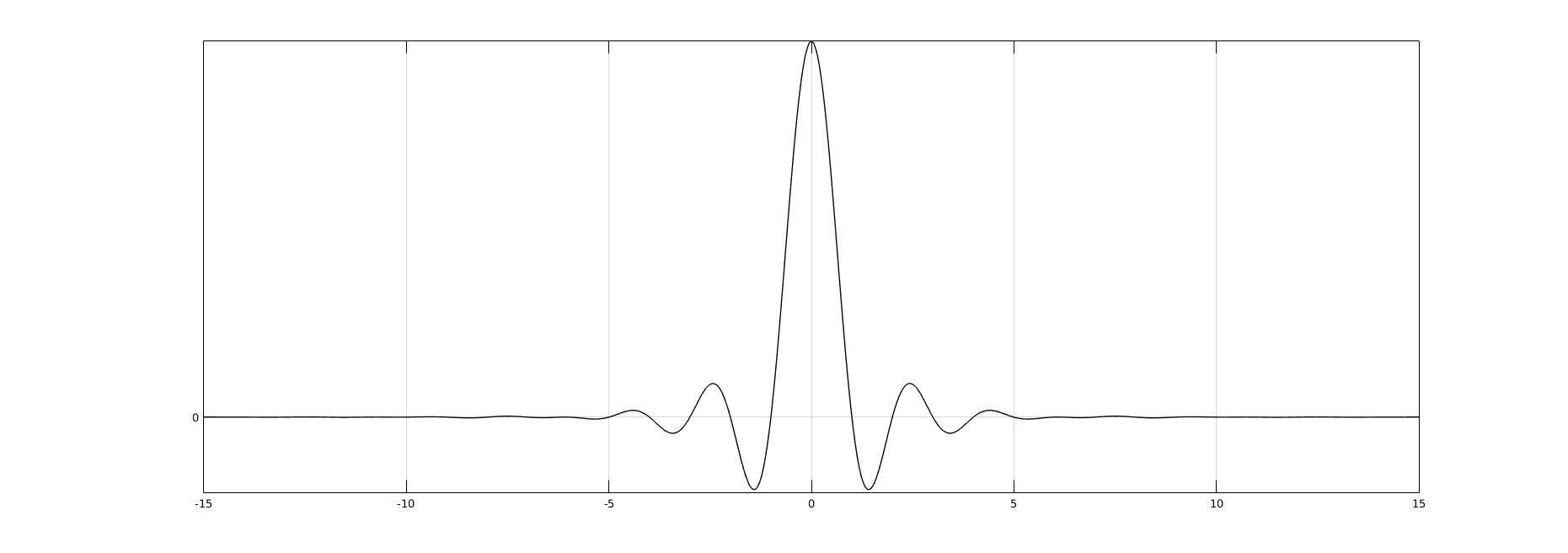
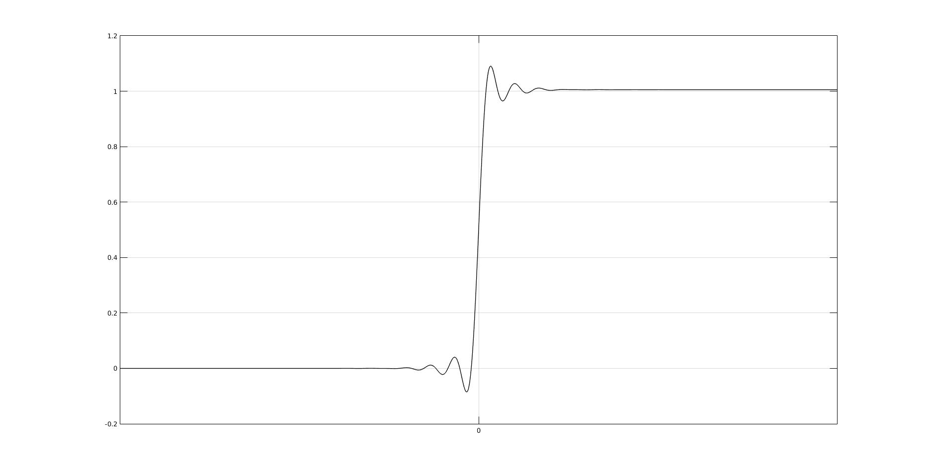
Figure 2.1. Representations of Dirac delta and Heaviside function

2.7. Functionally compact sets and multidimensional integration

2.7.1. Extreme value theorem and functionally compact sets

For GSF, suitable generalizations of many classical theorems of differential and integral calculus hold: intermediate value theorem, mean value theorems, suitable sheaf properties, local and global inverse function theorems, Banach fixed point theorem and a corresponding Picard-Lindelöf theorem both for ODE and PDE, see [25, 26, 27, 46, 28].

Even though the intervals $[a,b]\subseteq\mathchoice{{\vphantom{\mathbb{R}}}^{\scalebox{0.6}{$\rho$}}}{{\vphantom{\mathbb{R}}}^{\scalebox{0.56}{$\rho$}}}{{\vphantom{\mathbb{R}}}^{\scalebox{0.47}{$\rho$}}}{{\vphantom{\mathbb{R}}}^{\scalebox{0.35}{$\rho$}}}\widetilde{\mathbb{R}}$, $a$, $b\in\mathbb{R}$, are not compact in the sharp topology (see [24]), analogously to the case of smooth functions, a GSF satisfies an extreme value theorem on such sets. In fact, we have:

Theorem 25.

Let $f\in\mathcal{G}\mathcal{C}^{\infty}(X,\mathchoice{{\vphantom{\mathbb{R}}}^{\scalebox{0.6}{$\rho$}}}{{\vphantom{\mathbb{R}}}^{\scalebox{0.56}{$\rho$}}}{{\vphantom{\mathbb{R}}}^{\scalebox{0.47}{$\rho$}}}{{\vphantom{\mathbb{R}}}^{\scalebox{0.35}{$\rho$}}}\widetilde{\mathbb{R}})$ be a GSF defined on the subset $X$ of $\mathchoice{{\vphantom{\mathbb{R}}}^{\scalebox{0.6}{$\rho$}}}{{\vphantom{\mathbb{R}}}^{\scalebox{0.56}{$\rho$}}}{{\vphantom{\mathbb{R}}}^{\scalebox{0.47}{$\rho$}}}{{\vphantom{\mathbb{R}}}^{\scalebox{0.35}{$\rho$}}}\widetilde{\mathbb{R}}^{n}$. Let $\emptyset\neq K=[K_{\varepsilon}]\subseteq X$ be an internal set generated by a sharply bounded net $(K_{\varepsilon})$ of compact sets $K_{\varepsilon}\Subset\mathbb{R}^{n}$ , then

$$\exists m,M\in K\,\forall x\in K:\ f(m)\leq f(x)\leq f(M).$$ (2.8)

We shall use the assumptions on $K$ and $(K_{\varepsilon})$ given in this theorem to introduce a notion of “compact subset” which behaves better than the usual classical notion of compactness in the sharp topology.

Definition 26.

A subset $K$ of $\mathchoice{{\vphantom{\mathbb{R}}}^{\scalebox{0.6}{$\rho$}}}{{\vphantom{\mathbb{R}}}^{\scalebox{0.56}{$\rho$}}}{{\vphantom{\mathbb{R}}}^{\scalebox{0.47}{$\rho$}}}{{\vphantom{\mathbb{R}}}^{\scalebox{0.35}{$\rho$}}}\widetilde{\mathbb{R}}^{n}$ is called functionally compact, denoted by $K\Subset_{\text{\rm f}}\mathchoice{{\vphantom{\mathbb{R}}}^{\scalebox{0.6}{$\rho$}}}{{\vphantom{\mathbb{R}}}^{\scalebox{0.56}{$\rho$}}}{{\vphantom{\mathbb{R}}}^{\scalebox{0.47}{$\rho$}}}{{\vphantom{\mathbb{R}}}^{\scalebox{0.35}{$\rho$}}}\widetilde{\mathbb{R}}^{n}$, if there exists a net $(K_{\varepsilon})$ such that

1. $K=[K_{\varepsilon}]\subseteq\mathchoice{{\vphantom{\mathbb{R}}}^{\scalebox{0.6}{$\rho$}}}{{\vphantom{\mathbb{R}}}^{\scalebox{0.56}{$\rho$}}}{{\vphantom{\mathbb{R}}}^{\scalebox{0.47}{$\rho$}}}{{\vphantom{\mathbb{R}}}^{\scalebox{0.35}{$\rho$}}}\widetilde{\mathbb{R}}^{n}$.

2. $\exists R\in\mathchoice{{\vphantom{\mathbb{R}}}^{\scalebox{0.6}{$\rho$}}}{{\vphantom{\mathbb{R}}}^{\scalebox{0.56}{$\rho$}}}{{\vphantom{\mathbb{R}}}^{\scalebox{0.47}{$\rho$}}}{{\vphantom{\mathbb{R}}}^{\scalebox{0.35}{$\rho$}}}\widetilde{\mathbb{R}}_{>0}:\ K\subseteq B_{R}(0)$, i.e. $K$ is sharply bounded.

3. $\forall\varepsilon\in I:\ K_{\varepsilon}\Subset\mathbb{R}^{n}$.

If, in addition, $K\subseteq U\subseteq\mathchoice{{\vphantom{\mathbb{R}}}^{\scalebox{0.6}{$\rho$}}}{{\vphantom{\mathbb{R}}}^{\scalebox{0.56}{$\rho$}}}{{\vphantom{\mathbb{R}}}^{\scalebox{0.47}{$\rho$}}}{{\vphantom{\mathbb{R}}}^{\scalebox{0.35}{$\rho$}}}\widetilde{\mathbb{R}}^{n}$ then we write $K\Subset_{\text{\rm f}}U$. Finally, we write $[K_{\varepsilon}]\Subset_{\text{\rm f}}U$ if (ii), (iii) and $[K_{\varepsilon}]\subseteq U$ hold. Any net $(K_{\varepsilon})$ such that $[K_{\varepsilon}]=K$ is called a representative of $K$.

We motivate the name functionally compact subset by noting that on this type of subsets, GSF have properties very similar to those that ordinary smooth functions have on standard compact sets.

Remark 27.

1. By Thm. 11.(iii), any internal set $K=[K_{\varepsilon}]$ is closed in the sharp topology and hence functionally compact sets are always closed. In particular, the open interval $(0,1)\subseteq\mathchoice{{\vphantom{\mathbb{R}}}^{\scalebox{0.6}{$\rho$}}}{{\vphantom{\mathbb{R}}}^{\scalebox{0.56}{$\rho$}}}{{\vphantom{\mathbb{R}}}^{\scalebox{0.47}{$\rho$}}}{{\vphantom{\mathbb{R}}}^{\scalebox{0.35}{$\rho$}}}\widetilde{\mathbb{R}}$ is not functionally compact since it is not closed.

2. If $H\Subset\mathbb{R}^{n}$ is a non-empty ordinary compact set, then the internal set $[H]$ is functionally compact. In particular, $[0,1]=\left[[0,1]_{\mathbb{R}}\right]$ is functionally compact.

3. The empty set $\emptyset=\widetilde{\emptyset}\Subset_{\text{\rm f}}\mathchoice{{\vphantom{\mathbb{R}}}^{\scalebox{0.6}{$\rho$}}}{{\vphantom{\mathbb{R}}}^{\scalebox{0.56}{$\rho$}}}{{\vphantom{\mathbb{R}}}^{\scalebox{0.47}{$\rho$}}}{{\vphantom{\mathbb{R}}}^{\scalebox{0.35}{$\rho$}}}\widetilde{\mathbb{R}}$.

4. $\mathchoice{{\vphantom{\mathbb{R}}}^{\scalebox{0.6}{$\rho$}}}{{\vphantom{\mathbb{R}}}^{\scalebox{0.56}{$\rho$}}}{{\vphantom{\mathbb{R}}}^{\scalebox{0.47}{$\rho$}}}{{\vphantom{\mathbb{R}}}^{\scalebox{0.35}{$\rho$}}}\widetilde{\mathbb{R}}^{n}$ is not functionally compact since it is not sharply bounded.

5. The set of compactly supported points ${\text{\rm c}}({\mathbb{R}})$ is not functionally compact because the GSF $f(x)=x$ does not satisfy the conclusion (2.8) of Thm. 25.

In the present paper, we need the following properties of functionally compact sets.

Theorem 28.

1. Let $K\subseteq X\subseteq\mathchoice{{\vphantom{\mathbb{R}}}^{\scalebox{0.6}{$\rho$}}}{{\vphantom{\mathbb{R}}}^{\scalebox{0.56}{$\rho$}}}{{\vphantom{\mathbb{R}}}^{\scalebox{0.47}{$\rho$}}}{{\vphantom{\mathbb{R}}}^{\scalebox{0.35}{$\rho$}}}\widetilde{\mathbb{R}}^{n}$, $f\in\mathcal{G}\mathcal{C}^{\infty}(X,\mathchoice{{\vphantom{\mathbb{R}}}^{\scalebox{0.6}{$\rho$}}}{{\vphantom{\mathbb{R}}}^{\scalebox{0.56}{$\rho$}}}{{\vphantom{\mathbb{R}}}^{\scalebox{0.47}{$\rho$}}}{{\vphantom{\mathbb{R}}}^{\scalebox{0.35}{$\rho$}}}\widetilde{\mathbb{R}}^{d})$. Then $K\Subset_{\text{\rm f}}\mathchoice{{\vphantom{\mathbb{R}}}^{\scalebox{0.6}{$\rho$}}}{{\vphantom{\mathbb{R}}}^{\scalebox{0.56}{$\rho$}}}{{\vphantom{\mathbb{R}}}^{\scalebox{0.47}{$\rho$}}}{{\vphantom{\mathbb{R}}}^{\scalebox{0.35}{$\rho$}}}\widetilde{\mathbb{R}}^{n}$ implies $f(K)\Subset_{\text{\rm f}}\mathchoice{{\vphantom{\mathbb{R}}}^{\scalebox{0.6}{$\rho$}}}{{\vphantom{\mathbb{R}}}^{\scalebox{0.56}{$\rho$}}}{{\vphantom{\mathbb{R}}}^{\scalebox{0.47}{$\rho$}}}{{\vphantom{\mathbb{R}}}^{\scalebox{0.35}{$\rho$}}}\widetilde{\mathbb{R}}^{d}$.

2. Let $K$, $H\Subset_{\text{\rm f}}\mathchoice{{\vphantom{\mathbb{R}}}^{\scalebox{0.6}{$\rho$}}}{{\vphantom{\mathbb{R}}}^{\scalebox{0.56}{$\rho$}}}{{\vphantom{\mathbb{R}}}^{\scalebox{0.47}{$\rho$}}}{{\vphantom{\mathbb{R}}}^{\scalebox{0.35}{$\rho$}}}\widetilde{\mathbb{R}}^{n}$. If $K\cup H$ is an internal set, then it is a functionally compact set. If $K\cap H$ is an internal set, then it is a functionally compact set.

3. Let $H\subseteq K\Subset_{\text{\rm f}}\mathchoice{{\vphantom{\mathbb{R}}}^{\scalebox{0.6}{$\rho$}}}{{\vphantom{\mathbb{R}}}^{\scalebox{0.56}{$\rho$}}}{{\vphantom{\mathbb{R}}}^{\scalebox{0.47}{$\rho$}}}{{\vphantom{\mathbb{R}}}^{\scalebox{0.35}{$\rho$}}}\widetilde{\mathbb{R}}^{n}$, then if $H$ is an internal set, then $H\Subset_{\text{\rm f}}\mathchoice{{\vphantom{\mathbb{R}}}^{\scalebox{0.6}{$\rho$}}}{{\vphantom{\mathbb{R}}}^{\scalebox{0.56}{$\rho$}}}{{\vphantom{\mathbb{R}}}^{\scalebox{0.47}{$\rho$}}}{{\vphantom{\mathbb{R}}}^{\scalebox{0.35}{$\rho$}}}\widetilde{\mathbb{R}}^{n}$.

As a corollary of this theorem and Rem. (27).(ii) we get

Corollary 29.

If $a$, $b\in\mathchoice{{\vphantom{\mathbb{R}}}^{\scalebox{0.6}{$\rho$}}}{{\vphantom{\mathbb{R}}}^{\scalebox{0.56}{$\rho$}}}{{\vphantom{\mathbb{R}}}^{\scalebox{0.47}{$\rho$}}}{{\vphantom{\mathbb{R}}}^{\scalebox{0.35}{$\rho$}}}\widetilde{\mathbb{R}}$ and $a\leq b$, then $[a,b]\Subset_{\text{\rm f}}\mathchoice{{\vphantom{\mathbb{R}}}^{\scalebox{0.6}{$\rho$}}}{{\vphantom{\mathbb{R}}}^{\scalebox{0.56}{$\rho$}}}{{\vphantom{\mathbb{R}}}^{\scalebox{0.47}{$\rho$}}}{{\vphantom{\mathbb{R}}}^{\scalebox{0.35}{$\rho$}}}\widetilde{\mathbb{R}}$.

Let us note that $a$, $b\in\mathchoice{{\vphantom{\mathbb{R}}}^{\scalebox{0.6}{$\rho$}}}{{\vphantom{\mathbb{R}}}^{\scalebox{0.56}{$\rho$}}}{{\vphantom{\mathbb{R}}}^{\scalebox{0.47}{$\rho$}}}{{\vphantom{\mathbb{R}}}^{\scalebox{0.35}{$\rho$}}}\widetilde{\mathbb{R}}$ can also be infinite numbers, e.g. $a=\mathchoice{\hbox{\rm d}\rho}{\hbox{\rm d}\rho}{\scalebox{0.75}{$\hbox{\rm d}\rho$}}{\scalebox{0.35}{$\hbox{\rm d}\rho$}}^{-N}$, $b=\mathchoice{\hbox{\rm d}\rho}{\hbox{\rm d}\rho}{\scalebox{0.75}{$\hbox{\rm d}\rho$}}{\scalebox{0.35}{$\hbox{\rm d}\rho$}}^{-M}$ or $a=-\mathchoice{\hbox{\rm d}\rho}{\hbox{\rm d}\rho}{\scalebox{0.75}{$\hbox{\rm d}\rho$}}{\scalebox{0.35}{$\hbox{\rm d}\rho$}}^{-N}$, $b=\mathchoice{\hbox{\rm d}\rho}{\hbox{\rm d}\rho}{\scalebox{0.75}{$\hbox{\rm d}\rho$}}{\scalebox{0.35}{$\hbox{\rm d}\rho$}}^{-M}$ with $M>N$, so that e.g. $[-\mathchoice{\hbox{\rm d}\rho}{\hbox{\rm d}\rho}{\scalebox{0.75}{$\hbox{\rm d}\rho$}}{\scalebox{0.35}{$\hbox{\rm d}\rho$}}^{-N},\mathchoice{\hbox{\rm d}\rho}{\hbox{\rm d}\rho}{\scalebox{0.75}{$\hbox{\rm d}\rho$}}{\scalebox{0.35}{$\hbox{\rm d}\rho$}}^{-M}]\supseteq\mathbb{R}$. Finally, in the following result we consider the product of functionally compact sets:

Theorem 30.

Let $K\Subset_{\text{\rm f}}\mathchoice{{\vphantom{\mathbb{R}}}^{\scalebox{0.6}{$\rho$}}}{{\vphantom{\mathbb{R}}}^{\scalebox{0.56}{$\rho$}}}{{\vphantom{\mathbb{R}}}^{\scalebox{0.47}{$\rho$}}}{{\vphantom{\mathbb{R}}}^{\scalebox{0.35}{$\rho$}}}\widetilde{\mathbb{R}}^{n}$ and $H\Subset_{\text{\rm f}}\mathchoice{{\vphantom{\mathbb{R}}}^{\scalebox{0.6}{$\rho$}}}{{\vphantom{\mathbb{R}}}^{\scalebox{0.56}{$\rho$}}}{{\vphantom{\mathbb{R}}}^{\scalebox{0.47}{$\rho$}}}{{\vphantom{\mathbb{R}}}^{\scalebox{0.35}{$\rho$}}}\widetilde{\mathbb{R}}^{d}$, then $K\times H\Subset_{\text{\rm f}}\mathchoice{{\vphantom{\mathbb{R}}}^{\scalebox{0.6}{$\rho$}}}{{\vphantom{\mathbb{R}}}^{\scalebox{0.56}{$\rho$}}}{{\vphantom{\mathbb{R}}}^{\scalebox{0.47}{$\rho$}}}{{\vphantom{\mathbb{R}}}^{\scalebox{0.35}{$\rho$}}}\widetilde{\mathbb{R}}^{n+d}$. In particular, if $a_{i}\leq b_{i}$ for $i=1,\ldots,n$, then $\prod_{i=1}^{n}[a_{i},b_{i}]\Subset_{\text{\rm f}}\mathchoice{{\vphantom{\mathbb{R}}}^{\scalebox{0.6}{$\rho$}}}{{\vphantom{\mathbb{R}}}^{\scalebox{0.56}{$\rho$}}}{{\vphantom{\mathbb{R}}}^{\scalebox{0.47}{$\rho$}}}{{\vphantom{\mathbb{R}}}^{\scalebox{0.35}{$\rho$}}}\widetilde{\mathbb{R}}^{n}$.

Applying the extreme value theorem Thm. 25 to the first derivative, we also have the following

Theorem 31.

Let $a$, $b\in\mathchoice{{\vphantom{\mathbb{R}}}^{\scalebox{0.6}{$\rho$}}}{{\vphantom{\mathbb{R}}}^{\scalebox{0.56}{$\rho$}}}{{\vphantom{\mathbb{R}}}^{\scalebox{0.47}{$\rho$}}}{{\vphantom{\mathbb{R}}}^{\scalebox{0.35}{$\rho$}}}\widetilde{\mathbb{R}}^{n}$, $a<b$, $f\in{}^{\rho}\mathcal{G}\mathcal{C}^{\infty}([a,b],\mathchoice{{\vphantom{\mathbb{R}}}^{\scalebox{0.6}{$\rho$}}}{{\vphantom{\mathbb{R}}}^{\scalebox{0.56}{$\rho$}}}{{\vphantom{\mathbb{R}}}^{\scalebox{0.47}{$\rho$}}}{{\vphantom{\mathbb{R}}}^{\scalebox{0.35}{$\rho$}}}\widetilde{\mathbb{R}})$ be a GSF. Then

1. $\exists c\in[a,b]:\ f(b)-f(a)=(b-a)\cdot f^{\prime}(c)$.

2. Setting $M:=\max_{c\in[a,b]}\left|f^{\prime}(c)\right|\in\mathchoice{{\vphantom{\mathbb{R}}}^{\scalebox{0.6}{$\rho$}}}{{\vphantom{\mathbb{R}}}^{\scalebox{0.56}{$\rho$}}}{{\vphantom{\mathbb{R}}}^{\scalebox{0.47}{$\rho$}}}{{\vphantom{\mathbb{R}}}^{\scalebox{0.35}{$\rho$}}}\widetilde{\mathbb{R}}$, we hence have $\forall x,y\in[a,b]:\ \left|f(x)-f(y)\right|\leq M\cdot\left|x-y\right|$.

A theory of compactly supported GSF has been developed in [24], and it closely resembles the classical theory of LF-spaces of compactly supported smooth functions.

2.7.2. Multidimensional integration

Finally, to define FT of multivariable GSF we have to introduce multidimensional integration on suitable subsets of $\mathchoice{{\vphantom{\mathbb{R}}}^{\scalebox{0.6}{$\rho$}}}{{\vphantom{\mathbb{R}}}^{\scalebox{0.56}{$\rho$}}}{{\vphantom{\mathbb{R}}}^{\scalebox{0.47}{$\rho$}}}{{\vphantom{\mathbb{R}}}^{\scalebox{0.35}{$\rho$}}}\widetilde{\mathbb{R}}^{n}$ (see [27]).

Definition 32.

Let $\mu$ be a measure on $\mathbb{R}^{n}$ and let $K$ be a functionally compact subset of $\mathchoice{{\vphantom{\mathbb{R}}}^{\scalebox{0.6}{$\rho$}}}{{\vphantom{\mathbb{R}}}^{\scalebox{0.56}{$\rho$}}}{{\vphantom{\mathbb{R}}}^{\scalebox{0.47}{$\rho$}}}{{\vphantom{\mathbb{R}}}^{\scalebox{0.35}{$\rho$}}}\widetilde{\mathbb{R}}^{n}$. Then, we call $K$ $\mu$-measurable if the limit

$$\mu(K):=\lim_{m\to\infty}[\mu(\overline{B^{{\scriptscriptstyle\text{\rm E}}}}_{\rho_{\varepsilon}^{m}}(K_{\varepsilon}))]$$ (2.9)

exists for some representative $(K_{\varepsilon})$ of $K$. Here $m\in\mathbb{N}$, the limit is taken in the sharp topology on $\mathchoice{{\vphantom{\mathbb{R}}}^{\scalebox{0.6}{$\rho$}}}{{\vphantom{\mathbb{R}}}^{\scalebox{0.56}{$\rho$}}}{{\vphantom{\mathbb{R}}}^{\scalebox{0.47}{$\rho$}}}{{\vphantom{\mathbb{R}}}^{\scalebox{0.35}{$\rho$}}}\widetilde{\mathbb{R}}$, and $\overline{B^{{\scriptscriptstyle\text{\rm E}}}}_{r}(A):=\{x\in\mathbb{R}^{n}:d(x,A)\leq r\}$.

Let $K\Subset_{\text{\rm f}}\mathchoice{{\vphantom{\mathbb{R}}}^{\scalebox{0.6}{$\rho$}}}{{\vphantom{\mathbb{R}}}^{\scalebox{0.56}{$\rho$}}}{{\vphantom{\mathbb{R}}}^{\scalebox{0.47}{$\rho$}}}{{\vphantom{\mathbb{R}}}^{\scalebox{0.35}{$\rho$}}}\widetilde{\mathbb{R}}^{n}$. Let $(\Omega_{\varepsilon})$ be a net of open subsets of $\mathbb{R}^{n}$, and $(f_{\varepsilon})$ be a net of continuous maps $f_{\varepsilon}$: $\Omega_{\varepsilon}\longrightarrow\mathbb{R}$. Then we say that

$$(f_{\varepsilon})\textit{ defines a generalized integrable map}:K\longrightarrow\mathchoice{{\vphantom{\mathbb{R}}}^{\scalebox{0.6}{$\rho$}}}{{\vphantom{\mathbb{R}}}^{\scalebox{0.56}{$\rho$}}}{{\vphantom{\mathbb{R}}}^{\scalebox{0.47}{$\rho$}}}{{\vphantom{\mathbb{R}}}^{\scalebox{0.35}{$\rho$}}}\widetilde{\mathbb{R}}$$

if

1. $K\subseteq\langle\Omega_{\varepsilon}\rangle$ and $[f_{\varepsilon}(x_{\varepsilon})]\in\mathchoice{{\vphantom{\mathbb{R}}}^{\scalebox{0.6}{$\rho$}}}{{\vphantom{\mathbb{R}}}^{\scalebox{0.56}{$\rho$}}}{{\vphantom{\mathbb{R}}}^{\scalebox{0.47}{$\rho$}}}{{\vphantom{\mathbb{R}}}^{\scalebox{0.35}{$\rho$}}}\widetilde{\mathbb{R}}$ for all $[x_{\varepsilon}]\in K$.

2. $\forall(x_{\varepsilon}),(x^{\prime}_{\varepsilon})\in\mathbb{R}_{\rho}^{n}:\ [x_{\varepsilon}]=[x^{\prime}_{\varepsilon}]\in K\ \Rightarrow\ (f_{\varepsilon}(x_{\varepsilon}))\sim_{\rho}(f_{\varepsilon}(x^{\prime}_{\varepsilon}))$.

If $f\in\operatorname{{\bf Set}}(K,\mathchoice{{\vphantom{\mathbb{R}}}^{\scalebox{0.6}{$\rho$}}}{{\vphantom{\mathbb{R}}}^{\scalebox{0.56}{$\rho$}}}{{\vphantom{\mathbb{R}}}^{\scalebox{0.47}{$\rho$}}}{{\vphantom{\mathbb{R}}}^{\scalebox{0.35}{$\rho$}}}\widetilde{\mathbb{R}})$ is such that

$$\forall[x_{\varepsilon}]\in K:\ f\left([x_{\varepsilon}]\right)=\left[f_{\varepsilon}(x_{\varepsilon})\right]$$ (2.10)

we say that $f:K\longrightarrow\mathchoice{{\vphantom{\mathbb{R}}}^{\scalebox{0.6}{$\rho$}}}{{\vphantom{\mathbb{R}}}^{\scalebox{0.56}{$\rho$}}}{{\vphantom{\mathbb{R}}}^{\scalebox{0.47}{$\rho$}}}{{\vphantom{\mathbb{R}}}^{\scalebox{0.35}{$\rho$}}}\widetilde{\mathbb{R}}$ is a generalized integrable function.

We will again say that $f$ is defined by the net $(f_{\varepsilon})$ or that the net $(f_{\varepsilon})$ represents $f$. The set of all these generalized integrable functions will be denoted by $\mathchoice{{\vphantom{\mathcal{G}}}^{\scalebox{0.6}{$\rho$}}}{{\vphantom{\mathcal{G}}}^{\scalebox{0.56}{$\rho$}}}{{\vphantom{\mathcal{G}}}^{\scalebox{0.47}{$\rho$}}}{{\vphantom{\mathcal{G}}}^{\scalebox{0.35}{$\rho$}}}\mathcal{GI}(K,\mathchoice{{\vphantom{\mathbb{R}}}^{\scalebox{0.6}{$\rho$}}}{{\vphantom{\mathbb{R}}}^{\scalebox{0.56}{$\rho$}}}{{\vphantom{\mathbb{R}}}^{\scalebox{0.47}{$\rho$}}}{{\vphantom{\mathbb{R}}}^{\scalebox{0.35}{$\rho$}}}\widetilde{\mathbb{R}})$.

E.g., if $f=[f_{\varepsilon}(-)]|_{K}\in\mathchoice{{\vphantom{\mathcal{G}}}^{\scalebox{0.6}{$\rho$}}}{{\vphantom{\mathcal{G}}}^{\scalebox{0.56}{$\rho$}}}{{\vphantom{\mathcal{G}}}^{\scalebox{0.47}{$\rho$}}}{{\vphantom{\mathcal{G}}}^{\scalebox{0.35}{$\rho$}}}\mathcal{GC}^{\infty}(K,\mathchoice{{\vphantom{\mathbb{R}}}^{\scalebox{0.6}{$\rho$}}}{{\vphantom{\mathbb{R}}}^{\scalebox{0.56}{$\rho$}}}{{\vphantom{\mathbb{R}}}^{\scalebox{0.47}{$\rho$}}}{{\vphantom{\mathbb{R}}}^{\scalebox{0.35}{$\rho$}}}\widetilde{\mathbb{R}})$, then both $f$ and $|f|=[|f_{\varepsilon}(-)|]|_{K}$ are integrable on $K$ (but note that, in general, $|f|$ is not a GSF).

In the following result, we show that this definition generates a correct notion of multidimensional integration for GSF.

Theorem 33.

Let $K\subseteq\mathchoice{{\vphantom{\mathbb{R}}}^{\scalebox{0.6}{$\rho$}}}{{\vphantom{\mathbb{R}}}^{\scalebox{0.56}{$\rho$}}}{{\vphantom{\mathbb{R}}}^{\scalebox{0.47}{$\rho$}}}{{\vphantom{\mathbb{R}}}^{\scalebox{0.35}{$\rho$}}}\widetilde{\mathbb{R}}^{n}$ be $\mu$-measurable.

1. The definition of $\mu(K)$ is independent of the representative $(K_{\varepsilon})$.

2. There exists a representative $(K_{\varepsilon})$ of $K$ such that $\mu(K)=[\mu(K_{\varepsilon})]$.

3. Let $(K_{\varepsilon})$ be any representative of $K$ and let $f=[f_{\varepsilon}(-)]|_{K}\in\mathchoice{{\vphantom{\mathcal{G}}}^{\scalebox{0.6}{$\rho$}}}{{\vphantom{\mathcal{G}}}^{\scalebox{0.56}{$\rho$}}}{{\vphantom{\mathcal{G}}}^{\scalebox{0.47}{$\rho$}}}{{\vphantom{\mathcal{G}}}^{\scalebox{0.35}{$\rho$}}}\mathcal{GI}(K,\mathchoice{{\vphantom{\mathbb{R}}}^{\scalebox{0.6}{$\rho$}}}{{\vphantom{\mathbb{R}}}^{\scalebox{0.56}{$\rho$}}}{{\vphantom{\mathbb{R}}}^{\scalebox{0.47}{$\rho$}}}{{\vphantom{\mathbb{R}}}^{\scalebox{0.35}{$\rho$}}}\widetilde{\mathbb{R}})$. Then

   $$\int_{K}f\,\mathchoice{\hbox{\rm d}\mu}{\hbox{\rm d}\mu}{\scalebox{0.75}{$\hbox{\rm d}\mu$}}{\scalebox{0.35}{$\hbox{\rm d}\mu$}}:=\lim_{m\to\infty}\biggl{[}\int_{\overline{B^{{\scriptscriptstyle\text{\rm E}}}}_{\rho_{\varepsilon}^{m}}(K_{\varepsilon})}f_{\varepsilon}\,\mathchoice{\hbox{\rm d}\mu}{\hbox{\rm d}\mu}{\scalebox{0.75}{$\hbox{\rm d}\mu$}}{\scalebox{0.35}{$\hbox{\rm d}\mu$}}\biggr{]}\in\mathchoice{{\vphantom{\mathbb{R}}}^{\scalebox{0.6}{$\rho$}}}{{\vphantom{\mathbb{R}}}^{\scalebox{0.56}{$\rho$}}}{{\vphantom{\mathbb{R}}}^{\scalebox{0.47}{$\rho$}}}{{\vphantom{\mathbb{R}}}^{\scalebox{0.35}{$\rho$}}}\widetilde{\mathbb{R}}$$

   exists and its value is independent of the representative $(K_{\varepsilon})$.

4. There exists a representative $(K_{\varepsilon})$ of $K$ such that

   $$\int_{K}f\,\mathchoice{\hbox{\rm d}\mu}{\hbox{\rm d}\mu}{\scalebox{0.75}{$\hbox{\rm d}\mu$}}{\scalebox{0.35}{$\hbox{\rm d}\mu$}}=\biggl{[}\int_{K_{\varepsilon}}f_{\varepsilon}\,\mathchoice{\hbox{\rm d}\mu}{\hbox{\rm d}\mu}{\scalebox{0.75}{$\hbox{\rm d}\mu$}}{\scalebox{0.35}{$\hbox{\rm d}\mu$}}\biggr{]}\in\mathchoice{{\vphantom{\mathbb{R}}}^{\scalebox{0.6}{$\rho$}}}{{\vphantom{\mathbb{R}}}^{\scalebox{0.56}{$\rho$}}}{{\vphantom{\mathbb{R}}}^{\scalebox{0.47}{$\rho$}}}{{\vphantom{\mathbb{R}}}^{\scalebox{0.35}{$\rho$}}}\widetilde{\mathbb{R}}$$ (2.11)

   for each $f=[f_{\varepsilon}(-)]|_{K}\in\mathchoice{{\vphantom{\mathcal{G}}}^{\scalebox{0.6}{$\rho$}}}{{\vphantom{\mathcal{G}}}^{\scalebox{0.56}{$\rho$}}}{{\vphantom{\mathcal{G}}}^{\scalebox{0.47}{$\rho$}}}{{\vphantom{\mathcal{G}}}^{\scalebox{0.35}{$\rho$}}}\mathcal{GI}(K,\mathchoice{{\vphantom{\mathbb{R}}}^{\scalebox{0.6}{$\rho$}}}{{\vphantom{\mathbb{R}}}^{\scalebox{0.56}{$\rho$}}}{{\vphantom{\mathbb{R}}}^{\scalebox{0.47}{$\rho$}}}{{\vphantom{\mathbb{R}}}^{\scalebox{0.35}{$\rho$}}}\widetilde{\mathbb{R}})$. From (2.11), it also follows that $\left|\int_{K}f\,\mathchoice{\hbox{\rm d}\mu}{\hbox{\rm d}\mu}{\scalebox{0.75}{$\hbox{\rm d}\mu$}}{\scalebox{0.35}{$\hbox{\rm d}\mu$}}\right|\leq\int_{K}\left|f\right|\,\mathchoice{\hbox{\rm d}\mu}{\hbox{\rm d}\mu}{\scalebox{0.75}{$\hbox{\rm d}\mu$}}{\scalebox{0.35}{$\hbox{\rm d}\mu$}}$.

5. If $K=\prod_{i=1}^{n}[a_{i},b_{i}]$, then $K$ is $\lambda$-measurable ($\lambda$ being the Lebesgue measure on $\mathbb{R}^{n}$) and for all for each $f=[f_{\varepsilon}(-)]|_{K}\in\mathchoice{{\vphantom{\mathcal{G}}}^{\scalebox{0.6}{$\rho$}}}{{\vphantom{\mathcal{G}}}^{\scalebox{0.56}{$\rho$}}}{{\vphantom{\mathcal{G}}}^{\scalebox{0.47}{$\rho$}}}{{\vphantom{\mathcal{G}}}^{\scalebox{0.35}{$\rho$}}}\mathcal{GI}(K,\mathchoice{{\vphantom{\mathbb{R}}}^{\scalebox{0.6}{$\rho$}}}{{\vphantom{\mathbb{R}}}^{\scalebox{0.56}{$\rho$}}}{{\vphantom{\mathbb{R}}}^{\scalebox{0.47}{$\rho$}}}{{\vphantom{\mathbb{R}}}^{\scalebox{0.35}{$\rho$}}}\widetilde{\mathbb{R}})$ we have

   $$\int_{K}f\,\mathchoice{\hbox{\rm d}\lambda}{\hbox{\rm d}\lambda}{\scalebox{0.75}{$\hbox{\rm d}\lambda$}}{\scalebox{0.35}{$\hbox{\rm d}\lambda$}}=\left[\int_{a_{1,\varepsilon}}^{b_{1,\varepsilon}}\,dx_{1}\dots\int_{a_{n,\varepsilon}}^{b_{n,\varepsilon}}f_{\varepsilon}(x_{1},\dots,x_{n})\,\mathchoice{\hbox{\rm d}x_{n}}{\hbox{\rm d}x_{n}}{\scalebox{0.75}{$\hbox{\rm d}x_{n}$}}{\scalebox{0.35}{$\hbox{\rm d}x_{n}$}}\right]\in\mathchoice{{\vphantom{\mathbb{R}}}^{\scalebox{0.6}{$\rho$}}}{{\vphantom{\mathbb{R}}}^{\scalebox{0.56}{$\rho$}}}{{\vphantom{\mathbb{R}}}^{\scalebox{0.47}{$\rho$}}}{{\vphantom{\mathbb{R}}}^{\scalebox{0.35}{$\rho$}}}\widetilde{\mathbb{R}}$$ (2.12)

   for any representatives $(a_{i,\varepsilon})$, $(b_{i,\varepsilon})$ of $a_{i}$ and $b_{i}$ respectively. Therefore, if $n=1$, this notion of integral coincides with that of Thm. 16 and Def. 17. Note that (2.12) also directly implies Fubini’s theorem for this type of integrals.

6. Let $K\subseteq\mathchoice{{\vphantom{\mathbb{R}}}^{\scalebox{0.6}{$\rho$}}}{{\vphantom{\mathbb{R}}}^{\scalebox{0.56}{$\rho$}}}{{\vphantom{\mathbb{R}}}^{\scalebox{0.47}{$\rho$}}}{{\vphantom{\mathbb{R}}}^{\scalebox{0.35}{$\rho$}}}\widetilde{\mathbb{R}}^{n}$ be $\lambda$-measurable, where $\lambda$ is the Lebesgue measure, and let $\varphi\in\mathchoice{{\vphantom{\mathcal{G}}}^{\scalebox{0.6}{$\rho$}}}{{\vphantom{\mathcal{G}}}^{\scalebox{0.56}{$\rho$}}}{{\vphantom{\mathcal{G}}}^{\scalebox{0.47}{$\rho$}}}{{\vphantom{\mathcal{G}}}^{\scalebox{0.35}{$\rho$}}}\mathcal{GC}^{\infty}(K,\mathchoice{{\vphantom{\mathbb{R}}}^{\scalebox{0.6}{$\rho$}}}{{\vphantom{\mathbb{R}}}^{\scalebox{0.56}{$\rho$}}}{{\vphantom{\mathbb{R}}}^{\scalebox{0.47}{$\rho$}}}{{\vphantom{\mathbb{R}}}^{\scalebox{0.35}{$\rho$}}}\widetilde{\mathbb{R}}^{d})$ be such that $\varphi^{-1}\in\mathchoice{{\vphantom{\mathcal{G}}}^{\scalebox{0.6}{$\rho$}}}{{\vphantom{\mathcal{G}}}^{\scalebox{0.56}{$\rho$}}}{{\vphantom{\mathcal{G}}}^{\scalebox{0.47}{$\rho$}}}{{\vphantom{\mathcal{G}}}^{\scalebox{0.35}{$\rho$}}}\mathcal{GC}^{\infty}(\varphi(K),\mathchoice{{\vphantom{\mathbb{R}}}^{\scalebox{0.6}{$\rho$}}}{{\vphantom{\mathbb{R}}}^{\scalebox{0.56}{$\rho$}}}{{\vphantom{\mathbb{R}}}^{\scalebox{0.47}{$\rho$}}}{{\vphantom{\mathbb{R}}}^{\scalebox{0.35}{$\rho$}}}\widetilde{\mathbb{R}}^{n})$. Then $\varphi(K)$ is $\lambda$-measurable and

   $$\int_{\varphi(K)}f\,\mathchoice{\hbox{\rm d}\lambda}{\hbox{\rm d}\lambda}{\scalebox{0.75}{$\hbox{\rm d}\lambda$}}{\scalebox{0.35}{$\hbox{\rm d}\lambda$}}=\int_{K}(f\circ\varphi)\left|\det(\mathchoice{\hbox{\rm d}\varphi}{\hbox{\rm d}\varphi}{\scalebox{0.75}{$\hbox{\rm d}\varphi$}}{\scalebox{0.35}{$\hbox{\rm d}\varphi$}})\right|\,\mathchoice{\hbox{\rm d}\lambda}{\hbox{\rm d}\lambda}{\scalebox{0.75}{$\hbox{\rm d}\lambda$}}{\scalebox{0.35}{$\hbox{\rm d}\lambda$}}$$

   for each $f\in\mathchoice{{\vphantom{\mathcal{G}}}^{\scalebox{0.6}{$\rho$}}}{{\vphantom{\mathcal{G}}}^{\scalebox{0.56}{$\rho$}}}{{\vphantom{\mathcal{G}}}^{\scalebox{0.47}{$\rho$}}}{{\vphantom{\mathcal{G}}}^{\scalebox{0.35}{$\rho$}}}\mathcal{GI}(\varphi(K),\mathchoice{{\vphantom{\mathbb{R}}}^{\scalebox{0.6}{$\rho$}}}{{\vphantom{\mathbb{R}}}^{\scalebox{0.56}{$\rho$}}}{{\vphantom{\mathbb{R}}}^{\scalebox{0.47}{$\rho$}}}{{\vphantom{\mathbb{R}}}^{\scalebox{0.35}{$\rho$}}}\widetilde{\mathbb{R}})$.

In order to state a continuity property for this notion of integration, we have to introduce hypernatural numbers and hyperlimits as follows

Definition 34.

1. $\mathchoice{{\vphantom{\mathbb{N}}}^{\scalebox{0.6}{$\rho$}}}{{\vphantom{\mathbb{N}}}^{\scalebox{0.56}{$\rho$}}}{{\vphantom{\mathbb{N}}}^{\scalebox{0.47}{$\rho$}}}{{\vphantom{\mathbb{N}}}^{\scalebox{0.35}{$\rho$}}}\widetilde{\mathbb{N}}:=\left\{[n_{\varepsilon}]\in\mathchoice{{\vphantom{\mathbb{R}}}^{\scalebox{0.6}{$\rho$}}}{{\vphantom{\mathbb{R}}}^{\scalebox{0.56}{$\rho$}}}{{\vphantom{\mathbb{R}}}^{\scalebox{0.47}{$\rho$}}}{{\vphantom{\mathbb{R}}}^{\scalebox{0.35}{$\rho$}}}\widetilde{\mathbb{R}}\mid n_{\varepsilon}\in\mathbb{N}\ \forall\varepsilon\right\}$. Elements of $\mathchoice{{\vphantom{\mathbb{N}}}^{\scalebox{0.6}{$\rho$}}}{{\vphantom{\mathbb{N}}}^{\scalebox{0.56}{$\rho$}}}{{\vphantom{\mathbb{N}}}^{\scalebox{0.47}{$\rho$}}}{{\vphantom{\mathbb{N}}}^{\scalebox{0.35}{$\rho$}}}\widetilde{\mathbb{N}}$ are called hypernatural numbers or hyperfinite numbers. We clearly have $\mathbb{N}\subseteq\mathchoice{{\vphantom{\mathbb{N}}}^{\scalebox{0.6}{$\rho$}}}{{\vphantom{\mathbb{N}}}^{\scalebox{0.56}{$\rho$}}}{{\vphantom{\mathbb{N}}}^{\scalebox{0.47}{$\rho$}}}{{\vphantom{\mathbb{N}}}^{\scalebox{0.35}{$\rho$}}}\widetilde{\mathbb{N}}$, but among hypernatural numbers we also have infinite numbers.

2. $\mathbb{N}_{\rho}:=\left\{(n_{\varepsilon})\in\mathbb{R}_{\rho}\mid n_{\varepsilon}\in\mathbb{N}\ \forall\varepsilon\right\}$.

3. A map $x:\mathchoice{{\vphantom{\mathbb{N}}}^{\scalebox{0.6}{$\sigma$}}}{{\vphantom{\mathbb{N}}}^{\scalebox{0.56}{$\sigma$}}}{{\vphantom{\mathbb{N}}}^{\scalebox{0.47}{$\sigma$}}}{{\vphantom{\mathbb{N}}}^{\scalebox{0.35}{$\sigma$}}}\widetilde{\mathbb{N}}\longrightarrow\mathchoice{{\vphantom{\mathbb{R}}}^{\scalebox{0.6}{$\rho$}}}{{\vphantom{\mathbb{R}}}^{\scalebox{0.56}{$\rho$}}}{{\vphantom{\mathbb{R}}}^{\scalebox{0.47}{$\rho$}}}{{\vphantom{\mathbb{R}}}^{\scalebox{0.35}{$\rho$}}}\widetilde{\mathbb{R}}$, whose domain is the set of hyperfinite numbers $\mathchoice{{\vphantom{\mathbb{N}}}^{\scalebox{0.6}{$\sigma$}}}{{\vphantom{\mathbb{N}}}^{\scalebox{0.56}{$\sigma$}}}{{\vphantom{\mathbb{N}}}^{\scalebox{0.47}{$\sigma$}}}{{\vphantom{\mathbb{N}}}^{\scalebox{0.35}{$\sigma$}}}\widetilde{\mathbb{N}}$ is called a ($\sigma-$) hypersequence (of elements of $\mathchoice{{\vphantom{\mathbb{R}}}^{\scalebox{0.6}{$\rho$}}}{{\vphantom{\mathbb{R}}}^{\scalebox{0.56}{$\rho$}}}{{\vphantom{\mathbb{R}}}^{\scalebox{0.47}{$\rho$}}}{{\vphantom{\mathbb{R}}}^{\scalebox{0.35}{$\rho$}}}\widetilde{\mathbb{R}}$) and denoted by $(x_{n})_{n\in\mathchoice{{\vphantom{\mathbb{N}}}^{\scalebox{0.6}{$\sigma$}}}{{\vphantom{\mathbb{N}}}^{\scalebox{0.56}{$\sigma$}}}{{\vphantom{\mathbb{N}}}^{\scalebox{0.47}{$\sigma$}}}{{\vphantom{\mathbb{N}}}^{\scalebox{0.35}{$\sigma$}}}\widetilde{\mathbb{N}}}$, or simply $(x_{n})_{n}$ if the gauge on the domain is clear from the context. Let $\sigma$, $\rho$ be two gauges, $x:\mathchoice{{\vphantom{\mathbb{N}}}^{\scalebox{0.6}{$\sigma$}}}{{\vphantom{\mathbb{N}}}^{\scalebox{0.56}{$\sigma$}}}{{\vphantom{\mathbb{N}}}^{\scalebox{0.47}{$\sigma$}}}{{\vphantom{\mathbb{N}}}^{\scalebox{0.35}{$\sigma$}}}\widetilde{\mathbb{N}}\longrightarrow\mathchoice{{\vphantom{\mathbb{R}}}^{\scalebox{0.6}{$\rho$}}}{{\vphantom{\mathbb{R}}}^{\scalebox{0.56}{$\rho$}}}{{\vphantom{\mathbb{R}}}^{\scalebox{0.47}{$\rho$}}}{{\vphantom{\mathbb{R}}}^{\scalebox{0.35}{$\rho$}}}\widetilde{\mathbb{R}}$ be a hypersequence and $l\in\mathchoice{{\vphantom{\mathbb{R}}}^{\scalebox{0.6}{$\rho$}}}{{\vphantom{\mathbb{R}}}^{\scalebox{0.56}{$\rho$}}}{{\vphantom{\mathbb{R}}}^{\scalebox{0.47}{$\rho$}}}{{\vphantom{\mathbb{R}}}^{\scalebox{0.35}{$\rho$}}}\widetilde{\mathbb{R}}$. We say that $l$ is the hyperlimit of $(x_{n})_{n}$ as $n$$\rightarrow\infty$ and $n$$\in\mathchoice{{\vphantom{\mathbb{N}}}^{\scalebox{0.6}{$\sigma$}}}{{\vphantom{\mathbb{N}}}^{\scalebox{0.56}{$\sigma$}}}{{\vphantom{\mathbb{N}}}^{\scalebox{0.47}{$\sigma$}}}{{\vphantom{\mathbb{N}}}^{\scalebox{0.35}{$\sigma$}}}\widetilde{\mathbb{N}}$, if

   $$\forall q\in N\,\exists M\in\mathchoice{{\vphantom{\mathbb{N}}}^{\scalebox{0.6}{$\sigma$}}}{{\vphantom{\mathbb{N}}}^{\scalebox{0.56}{$\sigma$}}}{{\vphantom{\mathbb{N}}}^{\scalebox{0.47}{$\sigma$}}}{{\vphantom{\mathbb{N}}}^{\scalebox{0.35}{$\sigma$}}}\widetilde{\mathbb{N}}\,\forall n\in\mathchoice{{\vphantom{\mathbb{N}}}^{\scalebox{0.6}{$\sigma$}}}{{\vphantom{\mathbb{N}}}^{\scalebox{0.56}{$\sigma$}}}{{\vphantom{\mathbb{N}}}^{\scalebox{0.47}{$\sigma$}}}{{\vphantom{\mathbb{N}}}^{\scalebox{0.35}{$\sigma$}}}\widetilde{\mathbb{N}}_{\geq M}:\ |x_{n}-l|<\mathchoice{\hbox{\rm d}\rho}{\hbox{\rm d}\rho}{\scalebox{0.75}{$\hbox{\rm d}\rho$}}{\scalebox{0.35}{$\hbox{\rm d}\rho$}}^{q}.$$

   It can be easily proved that there exists at most one hyperlimit, and in this case it is denoted by $\mathchoice{\mathchoice{{\vphantom{\lim}}^{\scalebox{0.6}{$\raisebox{-0.35002pt}{$\rho$}$}}}{{\vphantom{\lim}}^{\scalebox{0.56}{$\raisebox{-0.35002pt}{$\rho$}$}}}{{\vphantom{\lim}}^{\scalebox{0.47}{$\raisebox{-0.35002pt}{$\rho$}$}}}{{\vphantom{\lim}}^{\scalebox{0.35}{$\raisebox{-0.35002pt}{$\rho$}$}}}\lim_{n\in\mathchoice{{\vphantom{\mathbb{N}}}^{\scalebox{0.6}{$\sigma$}}}{{\vphantom{\mathbb{N}}}^{\scalebox{0.56}{$\sigma$}}}{{\vphantom{\mathbb{N}}}^{\scalebox{0.47}{$\sigma$}}}{{\vphantom{\mathbb{N}}}^{\scalebox{0.35}{$\sigma$}}}\widetilde{\mathbb{N}}\,}}{\mathchoice{{\vphantom{\lim}}^{\scalebox{0.6}{$\rho$}}}{{\vphantom{\lim}}^{\scalebox{0.56}{$\rho$}}}{{\vphantom{\lim}}^{\scalebox{0.47}{$\rho$}}}{{\vphantom{\lim}}^{\scalebox{0.35}{$\rho$}}}\lim_{n\in\mathchoice{{\vphantom{\mathbb{N}}}^{\scalebox{0.6}{$\sigma$}}}{{\vphantom{\mathbb{N}}}^{\scalebox{0.56}{$\sigma$}}}{{\vphantom{\mathbb{N}}}^{\scalebox{0.47}{$\sigma$}}}{{\vphantom{\mathbb{N}}}^{\scalebox{0.35}{$\sigma$}}}\widetilde{\mathbb{N}}\,}}{\mathchoice{{\vphantom{\lim}}^{\scalebox{0.6}{$\rho$}}}{{\vphantom{\lim}}^{\scalebox{0.56}{$\rho$}}}{{\vphantom{\lim}}^{\scalebox{0.47}{$\rho$}}}{{\vphantom{\lim}}^{\scalebox{0.35}{$\rho$}}}\lim_{n\in\mathchoice{{\vphantom{\mathbb{N}}}^{\scalebox{0.6}{$\sigma$}}}{{\vphantom{\mathbb{N}}}^{\scalebox{0.56}{$\sigma$}}}{{\vphantom{\mathbb{N}}}^{\scalebox{0.47}{$\sigma$}}}{{\vphantom{\mathbb{N}}}^{\scalebox{0.35}{$\sigma$}}}\widetilde{\mathbb{N}}\,}}{\mathchoice{{\vphantom{\lim}}^{\scalebox{0.6}{$\rho$}}}{{\vphantom{\lim}}^{\scalebox{0.56}{$\rho$}}}{{\vphantom{\lim}}^{\scalebox{0.47}{$\rho$}}}{{\vphantom{\lim}}^{\scalebox{0.35}{$\rho$}}}\lim_{n\in\mathchoice{{\vphantom{\mathbb{N}}}^{\scalebox{0.6}{$\sigma$}}}{{\vphantom{\mathbb{N}}}^{\scalebox{0.56}{$\sigma$}}}{{\vphantom{\mathbb{N}}}^{\scalebox{0.47}{$\sigma$}}}{{\vphantom{\mathbb{N}}}^{\scalebox{0.35}{$\sigma$}}}\widetilde{\mathbb{N}}\,}}x_{n}=l$. Note that $\mathchoice{\hbox{\rm d}\rho}{\hbox{\rm d}\rho}{\scalebox{0.75}{$\hbox{\rm d}\rho$}}{\scalebox{0.35}{$\hbox{\rm d}\rho$}}<\frac{1}{n}$ if $n\in\mathbb{N}_{>0}$ so that $\frac{1}{n}\not\to 0$ in the sharp topology. On the contrary $\mathchoice{\mathchoice{{\vphantom{\lim}}^{\scalebox{0.6}{$\raisebox{-0.35002pt}{$\rho$}$}}}{{\vphantom{\lim}}^{\scalebox{0.56}{$\raisebox{-0.35002pt}{$\rho$}$}}}{{\vphantom{\lim}}^{\scalebox{0.47}{$\raisebox{-0.35002pt}{$\rho$}$}}}{{\vphantom{\lim}}^{\scalebox{0.35}{$\raisebox{-0.35002pt}{$\rho$}$}}}\lim_{n\in\mathchoice{{\vphantom{\mathbb{N}}}^{\scalebox{0.6}{$\rho$}}}{{\vphantom{\mathbb{N}}}^{\scalebox{0.56}{$\rho$}}}{{\vphantom{\mathbb{N}}}^{\scalebox{0.47}{$\rho$}}}{{\vphantom{\mathbb{N}}}^{\scalebox{0.35}{$\rho$}}}\widetilde{\mathbb{N}}\,}}{\mathchoice{{\vphantom{\lim}}^{\scalebox{0.6}{$\rho$}}}{{\vphantom{\lim}}^{\scalebox{0.56}{$\rho$}}}{{\vphantom{\lim}}^{\scalebox{0.47}{$\rho$}}}{{\vphantom{\lim}}^{\scalebox{0.35}{$\rho$}}}\lim_{n\in\mathchoice{{\vphantom{\mathbb{N}}}^{\scalebox{0.6}{$\rho$}}}{{\vphantom{\mathbb{N}}}^{\scalebox{0.56}{$\rho$}}}{{\vphantom{\mathbb{N}}}^{\scalebox{0.47}{$\rho$}}}{{\vphantom{\mathbb{N}}}^{\scalebox{0.35}{$\rho$}}}\widetilde{\mathbb{N}}\,}}{\mathchoice{{\vphantom{\lim}}^{\scalebox{0.6}{$\rho$}}}{{\vphantom{\lim}}^{\scalebox{0.56}{$\rho$}}}{{\vphantom{\lim}}^{\scalebox{0.47}{$\rho$}}}{{\vphantom{\lim}}^{\scalebox{0.35}{$\rho$}}}\lim_{n\in\mathchoice{{\vphantom{\mathbb{N}}}^{\scalebox{0.6}{$\rho$}}}{{\vphantom{\mathbb{N}}}^{\scalebox{0.56}{$\rho$}}}{{\vphantom{\mathbb{N}}}^{\scalebox{0.47}{$\rho$}}}{{\vphantom{\mathbb{N}}}^{\scalebox{0.35}{$\rho$}}}\widetilde{\mathbb{N}}\,}}{\mathchoice{{\vphantom{\lim}}^{\scalebox{0.6}{$\rho$}}}{{\vphantom{\lim}}^{\scalebox{0.56}{$\rho$}}}{{\vphantom{\lim}}^{\scalebox{0.47}{$\rho$}}}{{\vphantom{\lim}}^{\scalebox{0.35}{$\rho$}}}\lim_{n\in\mathchoice{{\vphantom{\mathbb{N}}}^{\scalebox{0.6}{$\rho$}}}{{\vphantom{\mathbb{N}}}^{\scalebox{0.56}{$\rho$}}}{{\vphantom{\mathbb{N}}}^{\scalebox{0.47}{$\rho$}}}{{\vphantom{\mathbb{N}}}^{\scalebox{0.35}{$\rho$}}}\widetilde{\mathbb{N}}\,}}\frac{1}{n}=0$ because $\mathchoice{{\vphantom{\mathbb{N}}}^{\scalebox{0.6}{$\rho$}}}{{\vphantom{\mathbb{N}}}^{\scalebox{0.56}{$\rho$}}}{{\vphantom{\mathbb{N}}}^{\scalebox{0.47}{$\rho$}}}{{\vphantom{\mathbb{N}}}^{\scalebox{0.35}{$\rho$}}}\widetilde{\mathbb{N}}$ contains arbitrarily large infinite hypernatural numbers.

The following continuity result once again underscores that functionally compact sets (even if they can be unbounded from a classical point of view) behaves as compact sets for GSF.

Theorem 35.

Let $K\subseteq\mathchoice{{\vphantom{\mathbb{R}}}^{\scalebox{0.6}{$\rho$}}}{{\vphantom{\mathbb{R}}}^{\scalebox{0.56}{$\rho$}}}{{\vphantom{\mathbb{R}}}^{\scalebox{0.47}{$\rho$}}}{{\vphantom{\mathbb{R}}}^{\scalebox{0.35}{$\rho$}}}\widetilde{\mathbb{R}}^{n}$ be a $\mu$-measurable functionally compact set and $f_{n}\in\mathchoice{{\vphantom{\mathcal{G}}}^{\scalebox{0.6}{$\rho$}}}{{\vphantom{\mathcal{G}}}^{\scalebox{0.56}{$\rho$}}}{{\vphantom{\mathcal{G}}}^{\scalebox{0.47}{$\rho$}}}{{\vphantom{\mathcal{G}}}^{\scalebox{0.35}{$\rho$}}}\mathcal{GC}^{\infty}(K,\mathchoice{{\vphantom{\mathbb{R}}}^{\scalebox{0.6}{$\rho$}}}{{\vphantom{\mathbb{R}}}^{\scalebox{0.56}{$\rho$}}}{{\vphantom{\mathbb{R}}}^{\scalebox{0.47}{$\rho$}}}{{\vphantom{\mathbb{R}}}^{\scalebox{0.35}{$\rho$}}}\widetilde{\mathbb{R}}^{d})$ for all $n\in\mathchoice{{\vphantom{\mathbb{N}}}^{\scalebox{0.6}{$\sigma$}}}{{\vphantom{\mathbb{N}}}^{\scalebox{0.56}{$\sigma$}}}{{\vphantom{\mathbb{N}}}^{\scalebox{0.47}{$\sigma$}}}{{\vphantom{\mathbb{N}}}^{\scalebox{0.35}{$\sigma$}}}\widetilde{\mathbb{N}}$. Then, if the hyperlimit $\mathchoice{\mathchoice{{\vphantom{\lim}}^{\scalebox{0.6}{$\raisebox{-0.35002pt}{$\rho$}$}}}{{\vphantom{\lim}}^{\scalebox{0.56}{$\raisebox{-0.35002pt}{$\rho$}$}}}{{\vphantom{\lim}}^{\scalebox{0.47}{$\raisebox{-0.35002pt}{$\rho$}$}}}{{\vphantom{\lim}}^{\scalebox{0.35}{$\raisebox{-0.35002pt}{$\rho$}$}}}\lim_{n\in\mathchoice{{\vphantom{\mathbb{N}}}^{\scalebox{0.6}{$\sigma$}}}{{\vphantom{\mathbb{N}}}^{\scalebox{0.56}{$\sigma$}}}{{\vphantom{\mathbb{N}}}^{\scalebox{0.47}{$\sigma$}}}{{\vphantom{\mathbb{N}}}^{\scalebox{0.35}{$\sigma$}}}\widetilde{\mathbb{N}}\,}}{\mathchoice{{\vphantom{\lim}}^{\scalebox{0.6}{$\rho$}}}{{\vphantom{\lim}}^{\scalebox{0.56}{$\rho$}}}{{\vphantom{\lim}}^{\scalebox{0.47}{$\rho$}}}{{\vphantom{\lim}}^{\scalebox{0.35}{$\rho$}}}\lim_{n\in\mathchoice{{\vphantom{\mathbb{N}}}^{\scalebox{0.6}{$\sigma$}}}{{\vphantom{\mathbb{N}}}^{\scalebox{0.56}{$\sigma$}}}{{\vphantom{\mathbb{N}}}^{\scalebox{0.47}{$\sigma$}}}{{\vphantom{\mathbb{N}}}^{\scalebox{0.35}{$\sigma$}}}\widetilde{\mathbb{N}}\,}}{\mathchoice{{\vphantom{\lim}}^{\scalebox{0.6}{$\rho$}}}{{\vphantom{\lim}}^{\scalebox{0.56}{$\rho$}}}{{\vphantom{\lim}}^{\scalebox{0.47}{$\rho$}}}{{\vphantom{\lim}}^{\scalebox{0.35}{$\rho$}}}\lim_{n\in\mathchoice{{\vphantom{\mathbb{N}}}^{\scalebox{0.6}{$\sigma$}}}{{\vphantom{\mathbb{N}}}^{\scalebox{0.56}{$\sigma$}}}{{\vphantom{\mathbb{N}}}^{\scalebox{0.47}{$\sigma$}}}{{\vphantom{\mathbb{N}}}^{\scalebox{0.35}{$\sigma$}}}\widetilde{\mathbb{N}}\,}}{\mathchoice{{\vphantom{\lim}}^{\scalebox{0.6}{$\rho$}}}{{\vphantom{\lim}}^{\scalebox{0.56}{$\rho$}}}{{\vphantom{\lim}}^{\scalebox{0.47}{$\rho$}}}{{\vphantom{\lim}}^{\scalebox{0.35}{$\rho$}}}\lim_{n\in\mathchoice{{\vphantom{\mathbb{N}}}^{\scalebox{0.6}{$\sigma$}}}{{\vphantom{\mathbb{N}}}^{\scalebox{0.56}{$\sigma$}}}{{\vphantom{\mathbb{N}}}^{\scalebox{0.47}{$\sigma$}}}{{\vphantom{\mathbb{N}}}^{\scalebox{0.35}{$\sigma$}}}\widetilde{\mathbb{N}}\,}}f_{n}(x)$ exists for each $x\in K$, then the convergence is uniform on $K$ and $\mathchoice{\mathchoice{{\vphantom{\lim}}^{\scalebox{0.6}{$\raisebox{-0.35002pt}{$\rho$}$}}}{{\vphantom{\lim}}^{\scalebox{0.56}{$\raisebox{-0.35002pt}{$\rho$}$}}}{{\vphantom{\lim}}^{\scalebox{0.47}{$\raisebox{-0.35002pt}{$\rho$}$}}}{{\vphantom{\lim}}^{\scalebox{0.35}{$\raisebox{-0.35002pt}{$\rho$}$}}}\lim_{n\in\mathchoice{{\vphantom{\mathbb{N}}}^{\scalebox{0.6}{$\sigma$}}}{{\vphantom{\mathbb{N}}}^{\scalebox{0.56}{$\sigma$}}}{{\vphantom{\mathbb{N}}}^{\scalebox{0.47}{$\sigma$}}}{{\vphantom{\mathbb{N}}}^{\scalebox{0.35}{$\sigma$}}}\widetilde{\mathbb{N}}\,}}{\mathchoice{{\vphantom{\lim}}^{\scalebox{0.6}{$\rho$}}}{{\vphantom{\lim}}^{\scalebox{0.56}{$\rho$}}}{{\vphantom{\lim}}^{\scalebox{0.47}{$\rho$}}}{{\vphantom{\lim}}^{\scalebox{0.35}{$\rho$}}}\lim_{n\in\mathchoice{{\vphantom{\mathbb{N}}}^{\scalebox{0.6}{$\sigma$}}}{{\vphantom{\mathbb{N}}}^{\scalebox{0.56}{$\sigma$}}}{{\vphantom{\mathbb{N}}}^{\scalebox{0.47}{$\sigma$}}}{{\vphantom{\mathbb{N}}}^{\scalebox{0.35}{$\sigma$}}}\widetilde{\mathbb{N}}\,}}{\mathchoice{{\vphantom{\lim}}^{\scalebox{0.6}{$\rho$}}}{{\vphantom{\lim}}^{\scalebox{0.56}{$\rho$}}}{{\vphantom{\lim}}^{\scalebox{0.47}{$\rho$}}}{{\vphantom{\lim}}^{\scalebox{0.35}{$\rho$}}}\lim_{n\in\mathchoice{{\vphantom{\mathbb{N}}}^{\scalebox{0.6}{$\sigma$}}}{{\vphantom{\mathbb{N}}}^{\scalebox{0.56}{$\sigma$}}}{{\vphantom{\mathbb{N}}}^{\scalebox{0.47}{$\sigma$}}}{{\vphantom{\mathbb{N}}}^{\scalebox{0.35}{$\sigma$}}}\widetilde{\mathbb{N}}\,}}{\mathchoice{{\vphantom{\lim}}^{\scalebox{0.6}{$\rho$}}}{{\vphantom{\lim}}^{\scalebox{0.56}{$\rho$}}}{{\vphantom{\lim}}^{\scalebox{0.47}{$\rho$}}}{{\vphantom{\lim}}^{\scalebox{0.35}{$\rho$}}}\lim_{n\in\mathchoice{{\vphantom{\mathbb{N}}}^{\scalebox{0.6}{$\sigma$}}}{{\vphantom{\mathbb{N}}}^{\scalebox{0.56}{$\sigma$}}}{{\vphantom{\mathbb{N}}}^{\scalebox{0.47}{$\sigma$}}}{{\vphantom{\mathbb{N}}}^{\scalebox{0.35}{$\sigma$}}}\widetilde{\mathbb{N}}\,}}f_{n}\in\mathchoice{{\vphantom{\mathcal{G}}}^{\scalebox{0.6}{$\rho$}}}{{\vphantom{\mathcal{G}}}^{\scalebox{0.56}{$\rho$}}}{{\vphantom{\mathcal{G}}}^{\scalebox{0.47}{$\rho$}}}{{\vphantom{\mathcal{G}}}^{\scalebox{0.35}{$\rho$}}}\mathcal{GC}^{\infty}(K,\mathchoice{{\vphantom{\mathbb{R}}}^{\scalebox{0.6}{$\rho$}}}{{\vphantom{\mathbb{R}}}^{\scalebox{0.56}{$\rho$}}}{{\vphantom{\mathbb{R}}}^{\scalebox{0.47}{$\rho$}}}{{\vphantom{\mathbb{R}}}^{\scalebox{0.35}{$\rho$}}}\widetilde{\mathbb{R}}^{d})$. Finally

$$\mathchoice{\mathchoice{{\vphantom{\lim}}^{\scalebox{0.6}{$\raisebox{-0.35002pt}{$\rho$}$}}}{{\vphantom{\lim}}^{\scalebox{0.56}{$\raisebox{-0.35002pt}{$\rho$}$}}}{{\vphantom{\lim}}^{\scalebox{0.47}{$\raisebox{-0.35002pt}{$\rho$}$}}}{{\vphantom{\lim}}^{\scalebox{0.35}{$\raisebox{-0.35002pt}{$\rho$}$}}}\lim_{n\in\mathchoice{{\vphantom{\mathbb{N}}}^{\scalebox{0.6}{$\sigma$}}}{{\vphantom{\mathbb{N}}}^{\scalebox{0.56}{$\sigma$}}}{{\vphantom{\mathbb{N}}}^{\scalebox{0.47}{$\sigma$}}}{{\vphantom{\mathbb{N}}}^{\scalebox{0.35}{$\sigma$}}}\widetilde{\mathbb{N}}\,}}{\mathchoice{{\vphantom{\lim}}^{\scalebox{0.6}{$\rho$}}}{{\vphantom{\lim}}^{\scalebox{0.56}{$\rho$}}}{{\vphantom{\lim}}^{\scalebox{0.47}{$\rho$}}}{{\vphantom{\lim}}^{\scalebox{0.35}{$\rho$}}}\lim_{n\in\mathchoice{{\vphantom{\mathbb{N}}}^{\scalebox{0.6}{$\sigma$}}}{{\vphantom{\mathbb{N}}}^{\scalebox{0.56}{$\sigma$}}}{{\vphantom{\mathbb{N}}}^{\scalebox{0.47}{$\sigma$}}}{{\vphantom{\mathbb{N}}}^{\scalebox{0.35}{$\sigma$}}}\widetilde{\mathbb{N}}\,}}{\mathchoice{{\vphantom{\lim}}^{\scalebox{0.6}{$\rho$}}}{{\vphantom{\lim}}^{\scalebox{0.56}{$\rho$}}}{{\vphantom{\lim}}^{\scalebox{0.47}{$\rho$}}}{{\vphantom{\lim}}^{\scalebox{0.35}{$\rho$}}}\lim_{n\in\mathchoice{{\vphantom{\mathbb{N}}}^{\scalebox{0.6}{$\sigma$}}}{{\vphantom{\mathbb{N}}}^{\scalebox{0.56}{$\sigma$}}}{{\vphantom{\mathbb{N}}}^{\scalebox{0.47}{$\sigma$}}}{{\vphantom{\mathbb{N}}}^{\scalebox{0.35}{$\sigma$}}}\widetilde{\mathbb{N}}\,}}{\mathchoice{{\vphantom{\lim}}^{\scalebox{0.6}{$\rho$}}}{{\vphantom{\lim}}^{\scalebox{0.56}{$\rho$}}}{{\vphantom{\lim}}^{\scalebox{0.47}{$\rho$}}}{{\vphantom{\lim}}^{\scalebox{0.35}{$\rho$}}}\lim_{n\in\mathchoice{{\vphantom{\mathbb{N}}}^{\scalebox{0.6}{$\sigma$}}}{{\vphantom{\mathbb{N}}}^{\scalebox{0.56}{$\sigma$}}}{{\vphantom{\mathbb{N}}}^{\scalebox{0.47}{$\sigma$}}}{{\vphantom{\mathbb{N}}}^{\scalebox{0.35}{$\sigma$}}}\widetilde{\mathbb{N}}\,}}\int_{K}f_{n}\,\mathchoice{\hbox{\rm d}x_{n}}{\hbox{\rm d}x_{n}}{\scalebox{0.75}{$\hbox{\rm d}x_{n}$}}{\scalebox{0.35}{$\hbox{\rm d}x_{n}$}}=\int_{K}\mathchoice{\mathchoice{{\vphantom{\lim}}^{\scalebox{0.6}{$\raisebox{-0.35002pt}{$\rho$}$}}}{{\vphantom{\lim}}^{\scalebox{0.56}{$\raisebox{-0.35002pt}{$\rho$}$}}}{{\vphantom{\lim}}^{\scalebox{0.47}{$\raisebox{-0.35002pt}{$\rho$}$}}}{{\vphantom{\lim}}^{\scalebox{0.35}{$\raisebox{-0.35002pt}{$\rho$}$}}}\lim_{n\in\mathchoice{{\vphantom{\mathbb{N}}}^{\scalebox{0.6}{$\sigma$}}}{{\vphantom{\mathbb{N}}}^{\scalebox{0.56}{$\sigma$}}}{{\vphantom{\mathbb{N}}}^{\scalebox{0.47}{$\sigma$}}}{{\vphantom{\mathbb{N}}}^{\scalebox{0.35}{$\sigma$}}}\widetilde{\mathbb{N}}\,}}{\mathchoice{{\vphantom{\lim}}^{\scalebox{0.6}{$\rho$}}}{{\vphantom{\lim}}^{\scalebox{0.56}{$\rho$}}}{{\vphantom{\lim}}^{\scalebox{0.47}{$\rho$}}}{{\vphantom{\lim}}^{\scalebox{0.35}{$\rho$}}}\lim_{n\in\mathchoice{{\vphantom{\mathbb{N}}}^{\scalebox{0.6}{$\sigma$}}}{{\vphantom{\mathbb{N}}}^{\scalebox{0.56}{$\sigma$}}}{{\vphantom{\mathbb{N}}}^{\scalebox{0.47}{$\sigma$}}}{{\vphantom{\mathbb{N}}}^{\scalebox{0.35}{$\sigma$}}}\widetilde{\mathbb{N}}\,}}{\mathchoice{{\vphantom{\lim}}^{\scalebox{0.6}{$\rho$}}}{{\vphantom{\lim}}^{\scalebox{0.56}{$\rho$}}}{{\vphantom{\lim}}^{\scalebox{0.47}{$\rho$}}}{{\vphantom{\lim}}^{\scalebox{0.35}{$\rho$}}}\lim_{n\in\mathchoice{{\vphantom{\mathbb{N}}}^{\scalebox{0.6}{$\sigma$}}}{{\vphantom{\mathbb{N}}}^{\scalebox{0.56}{$\sigma$}}}{{\vphantom{\mathbb{N}}}^{\scalebox{0.47}{$\sigma$}}}{{\vphantom{\mathbb{N}}}^{\scalebox{0.35}{$\sigma$}}}\widetilde{\mathbb{N}}\,}}{\mathchoice{{\vphantom{\lim}}^{\scalebox{0.6}{$\rho$}}}{{\vphantom{\lim}}^{\scalebox{0.56}{$\rho$}}}{{\vphantom{\lim}}^{\scalebox{0.47}{$\rho$}}}{{\vphantom{\lim}}^{\scalebox{0.35}{$\rho$}}}\lim_{n\in\mathchoice{{\vphantom{\mathbb{N}}}^{\scalebox{0.6}{$\sigma$}}}{{\vphantom{\mathbb{N}}}^{\scalebox{0.56}{$\sigma$}}}{{\vphantom{\mathbb{N}}}^{\scalebox{0.47}{$\sigma$}}}{{\vphantom{\mathbb{N}}}^{\scalebox{0.35}{$\sigma$}}}\widetilde{\mathbb{N}}\,}}f_{n}\,\mathchoice{\hbox{\rm d}x_{n}}{\hbox{\rm d}x_{n}}{\scalebox{0.75}{$\hbox{\rm d}x_{n}$}}{\scalebox{0.35}{$\hbox{\rm d}x_{n}$}}.$$ (2.13)

For the proof of this theorem see [27], and for the notion of hyperlimit see [47].

3. Convolution on $\mathchoice{{\vphantom{\mathbb{R}}}^{\scalebox{0.6}{$\rho$}}}{{\vphantom{\mathbb{R}}}^{\scalebox{0.56}{$\rho$}}}{{\vphantom{\mathbb{R}}}^{\scalebox{0.47}{$\rho$}}}{{\vphantom{\mathbb{R}}}^{\scalebox{0.35}{$\rho$}}}\widetilde{\mathbb{R}}^{n}$

In this section, we define and study convolution $f*g$ of two GSF, where $f$ or $g$ is compactly supported. Compactly supported GSF were introduced in [24] for the gauge $\rho_{\varepsilon}=\varepsilon$. For an arbitrary gauge, we here define and study the notions needed for the HFT as well as for the study of convolution of GSF.

Definition 36.

Assume that $X\subseteq\mathchoice{{\vphantom{\mathbb{R}}}^{\scalebox{0.6}{$\rho$}}}{{\vphantom{\mathbb{R}}}^{\scalebox{0.56}{$\rho$}}}{{\vphantom{\mathbb{R}}}^{\scalebox{0.47}{$\rho$}}}{{\vphantom{\mathbb{R}}}^{\scalebox{0.35}{$\rho$}}}\widetilde{\mathbb{R}}^{n}$, $Y\subseteq\mathchoice{{\vphantom{\mathbb{R}}}^{\scalebox{0.6}{$\rho$}}}{{\vphantom{\mathbb{R}}}^{\scalebox{0.56}{$\rho$}}}{{\vphantom{\mathbb{R}}}^{\scalebox{0.47}{$\rho$}}}{{\vphantom{\mathbb{R}}}^{\scalebox{0.35}{$\rho$}}}\widetilde{\mathbb{R}}^{d}$ and $f\in\mathchoice{{\vphantom{\mathcal{G}}}^{\scalebox{0.6}{$\rho$}}}{{\vphantom{\mathcal{G}}}^{\scalebox{0.56}{$\rho$}}}{{\vphantom{\mathcal{G}}}^{\scalebox{0.47}{$\rho$}}}{{\vphantom{\mathcal{G}}}^{\scalebox{0.35}{$\rho$}}}\mathcal{GC}^{\infty}\left(X,Y\right)$, then

1. $\text{supp}\left(f\right):=\overline{\left\{x\in X\mid\left|f\left(x\right)\right|>0\right\}}$, where $\overline{\left(\cdot\right)}$ denotes the relative closure in $X$ with respect to the sharp topology, is called the support of $f$. We recall (see just after Def. 1 and Lem. 4) that $x>0$ means that $x\in\mathchoice{{\vphantom{\mathbb{R}}}^{\scalebox{0.6}{$\rho$}}}{{\vphantom{\mathbb{R}}}^{\scalebox{0.56}{$\rho$}}}{{\vphantom{\mathbb{R}}}^{\scalebox{0.47}{$\rho$}}}{{\vphantom{\mathbb{R}}}^{\scalebox{0.35}{$\rho$}}}\widetilde{\mathbb{R}}_{\geq 0}$ is positive and invertible.

2. For $A\subseteq\mathchoice{{\vphantom{\mathbb{R}}}^{\scalebox{0.6}{$\rho$}}}{{\vphantom{\mathbb{R}}}^{\scalebox{0.56}{$\rho$}}}{{\vphantom{\mathbb{R}}}^{\scalebox{0.47}{$\rho$}}}{{\vphantom{\mathbb{R}}}^{\scalebox{0.35}{$\rho$}}}\widetilde{\mathbb{R}}$ we call the set $\text{ext}\left(A\right):=\left\{x\in\mathchoice{{\vphantom{\mathbb{R}}}^{\scalebox{0.6}{$\rho$}}}{{\vphantom{\mathbb{R}}}^{\scalebox{0.56}{$\rho$}}}{{\vphantom{\mathbb{R}}}^{\scalebox{0.47}{$\rho$}}}{{\vphantom{\mathbb{R}}}^{\scalebox{0.35}{$\rho$}}}\widetilde{\mathbb{R}}\mid\forall a\in A:\ \left|x-a\right|>0\right\}$ the strong exterior of $A$. Recalling Lem. 4, if $x\in\text{ext}(A)$, then $|x-a|\geq\mathchoice{\hbox{\rm d}\rho}{\hbox{\rm d}\rho}{\scalebox{0.75}{$\hbox{\rm d}\rho$}}{\scalebox{0.35}{$\hbox{\rm d}\rho$}}^{q}$ for all $a\in A$ and for some $q=q(a)\in\mathbb{N}$.

3. Let $H\Subset_{\text{\rm f}}\mathchoice{{\vphantom{\mathbb{R}}}^{\scalebox{0.6}{$\rho$}}}{{\vphantom{\mathbb{R}}}^{\scalebox{0.56}{$\rho$}}}{{\vphantom{\mathbb{R}}}^{\scalebox{0.47}{$\rho$}}}{{\vphantom{\mathbb{R}}}^{\scalebox{0.35}{$\rho$}}}\widetilde{\mathbb{R}}^{n}$, we say that $f\in\mathchoice{{\vphantom{\mathcal{D}}}^{\scalebox{0.6}{$\rho$}}}{{\vphantom{\mathcal{D}}}^{\scalebox{0.56}{$\rho$}}}{{\vphantom{\mathcal{D}}}^{\scalebox{0.47}{$\rho$}}}{{\vphantom{\mathcal{D}}}^{\scalebox{0.35}{$\rho$}}}\mathcal{GD}\left(H,Y\right)$ if $f\in\mathchoice{{\vphantom{\mathcal{G}}}^{\scalebox{0.6}{$\rho$}}}{{\vphantom{\mathcal{G}}}^{\scalebox{0.56}{$\rho$}}}{{\vphantom{\mathcal{G}}}^{\scalebox{0.47}{$\rho$}}}{{\vphantom{\mathcal{G}}}^{\scalebox{0.35}{$\rho$}}}\mathcal{GC}^{\infty}(\mathchoice{{\vphantom{\mathbb{R}}}^{\scalebox{0.6}{$\rho$}}}{{\vphantom{\mathbb{R}}}^{\scalebox{0.56}{$\rho$}}}{{\vphantom{\mathbb{R}}}^{\scalebox{0.47}{$\rho$}}}{{\vphantom{\mathbb{R}}}^{\scalebox{0.35}{$\rho$}}}\widetilde{\mathbb{R}}^{n},Y)$ and $\text{supp}\left(f\right)\subseteq H$. We say that $f\in\mathchoice{{\vphantom{\mathcal{D}}}^{\scalebox{0.6}{$\rho$}}}{{\vphantom{\mathcal{D}}}^{\scalebox{0.56}{$\rho$}}}{{\vphantom{\mathcal{D}}}^{\scalebox{0.47}{$\rho$}}}{{\vphantom{\mathcal{D}}}^{\scalebox{0.35}{$\rho$}}}\mathcal{GD}(\mathchoice{{\vphantom{\mathbb{R}}}^{\scalebox{0.6}{$\rho$}}}{{\vphantom{\mathbb{R}}}^{\scalebox{0.56}{$\rho$}}}{{\vphantom{\mathbb{R}}}^{\scalebox{0.47}{$\rho$}}}{{\vphantom{\mathbb{R}}}^{\scalebox{0.35}{$\rho$}}}\widetilde{\mathbb{R}}^{n},Y)$ if $f\in\mathchoice{{\vphantom{\mathcal{D}}}^{\scalebox{0.6}{$\rho$}}}{{\vphantom{\mathcal{D}}}^{\scalebox{0.56}{$\rho$}}}{{\vphantom{\mathcal{D}}}^{\scalebox{0.47}{$\rho$}}}{{\vphantom{\mathcal{D}}}^{\scalebox{0.35}{$\rho$}}}\mathcal{GD}\left(H,Y\right)$ for some $H\Subset_{\text{\rm f}}\mathchoice{{\vphantom{\mathbb{R}}}^{\scalebox{0.6}{$\rho$}}}{{\vphantom{\mathbb{R}}}^{\scalebox{0.56}{$\rho$}}}{{\vphantom{\mathbb{R}}}^{\scalebox{0.47}{$\rho$}}}{{\vphantom{\mathbb{R}}}^{\scalebox{0.35}{$\rho$}}}\widetilde{\mathbb{R}}^{n}$. Such an $f$ is called compactly supported; for simplicity we set $\mathchoice{{\vphantom{\mathcal{D}}}^{\scalebox{0.6}{$\rho$}}}{{\vphantom{\mathcal{D}}}^{\scalebox{0.56}{$\rho$}}}{{\vphantom{\mathcal{D}}}^{\scalebox{0.47}{$\rho$}}}{{\vphantom{\mathcal{D}}}^{\scalebox{0.35}{$\rho$}}}\mathcal{GD}(H):=\mathchoice{{\vphantom{\mathcal{D}}}^{\scalebox{0.6}{$\rho$}}}{{\vphantom{\mathcal{D}}}^{\scalebox{0.56}{$\rho$}}}{{\vphantom{\mathcal{D}}}^{\scalebox{0.47}{$\rho$}}}{{\vphantom{\mathcal{D}}}^{\scalebox{0.35}{$\rho$}}}\mathcal{GD}(H,\mathchoice{{\vphantom{\mathbb{C}}}^{\scalebox{0.6}{$\rho$}}}{{\vphantom{\mathbb{C}}}^{\scalebox{0.56}{$\rho$}}}{{\vphantom{\mathbb{C}}}^{\scalebox{0.47}{$\rho$}}}{{\vphantom{\mathbb{C}}}^{\scalebox{0.35}{$\rho$}}}\widetilde{\mathbb{C}})$. Note that $\text{supp}(f)$ is clearly always closed, and if $f\in\mathchoice{{\vphantom{\mathcal{D}}}^{\scalebox{0.6}{$\rho$}}}{{\vphantom{\mathcal{D}}}^{\scalebox{0.56}{$\rho$}}}{{\vphantom{\mathcal{D}}}^{\scalebox{0.47}{$\rho$}}}{{\vphantom{\mathcal{D}}}^{\scalebox{0.35}{$\rho$}}}\mathcal{GD}\left(H,Y\right)$ then it is also sharply bounded. However, in general it is not an internal set so it is not a functionally compact set. Accordingly, the theory of multidimensional integration of Sec. 2.7.2 does not allow us to consider $\int_{\text{supp}(f)}f$ even if $f$ is compactly supported.

Remark 37.

1. Note that the notion of standard support $\text{stsupp}\left(f\right)$ as defined in Thm. 22 and the present notion $\text{supp}\left(f\right)$ of support, as defined above, are different. The main distinction is that $\text{stsupp}\left(f\right)\subseteq\mathbb{R}^{n}$ while $\text{supp}\left(f\right)\subseteq\mathchoice{{\vphantom{\mathbb{R}}}^{\scalebox{0.6}{$\rho$}}}{{\vphantom{\mathbb{R}}}^{\scalebox{0.56}{$\rho$}}}{{\vphantom{\mathbb{R}}}^{\scalebox{0.47}{$\rho$}}}{{\vphantom{\mathbb{R}}}^{\scalebox{0.35}{$\rho$}}}\widetilde{\mathbb{R}}^{n}$. Moreover if we consider a CGF $f\in\mathchoice{{\vphantom{\mathcal{G}}}^{\scalebox{0.6}{$\rho$}}}{{\vphantom{\mathcal{G}}}^{\scalebox{0.56}{$\rho$}}}{{\vphantom{\mathcal{G}}}^{\scalebox{0.47}{$\rho$}}}{{\vphantom{\mathcal{G}}}^{\scalebox{0.35}{$\rho$}}}\mathcal{GC}^{\infty}({\text{\rm c}}({\Omega}),\mathchoice{{\vphantom{\mathbb{R}}}^{\scalebox{0.6}{$\rho$}}}{{\vphantom{\mathbb{R}}}^{\scalebox{0.56}{$\rho$}}}{{\vphantom{\mathbb{R}}}^{\scalebox{0.47}{$\rho$}}}{{\vphantom{\mathbb{R}}}^{\scalebox{0.35}{$\rho$}}}\widetilde{\mathbb{R}}^{d})$, then $\text{supp}\left(f\right)\cap\Omega\subseteq\text{stsupp}\left(f\right)$.

2. Since $\delta\left(0\right)>0$ then $\delta|_{B_{r}\left(0\right)}>0$ for some $r\in\mathchoice{{\vphantom{\mathbb{R}}}^{\scalebox{0.6}{$\rho$}}}{{\vphantom{\mathbb{R}}}^{\scalebox{0.56}{$\rho$}}}{{\vphantom{\mathbb{R}}}^{\scalebox{0.47}{$\rho$}}}{{\vphantom{\mathbb{R}}}^{\scalebox{0.35}{$\rho$}}}\widetilde{\mathbb{R}}_{>0}$ by the sharp continuity of $\delta$, i.e. Thm. 13.(ii), hence $B_{r}\left(0\right)\subseteq\text{supp}\left(\delta\right)$, whereas $\text{stsupp}\left(\delta\right)=\left\{0\right\}$. Example 24.(i) also yields that $\text{supp}(\delta)\subseteq[-r,r]^{n}$ for all $r\in\mathbb{R}_{>0}$.

3. Any rapidly decreasing function $f\in\mathcal{S}(\mathbb{R}^{n})$ satisfies the inequality $0\leq f\left(x\right)\leq\left|x\right|^{-q}$, $\forall q\in\mathbb{N}$, for $\left|x\right|$ finite sufficiently large. Therefore, for all strongly infinite $x$, we have $f\left(x\right)=0$ i.e., $f\in\mathchoice{{\vphantom{\mathcal{D}}}^{\scalebox{0.6}{$\rho$}}}{{\vphantom{\mathcal{D}}}^{\scalebox{0.56}{$\rho$}}}{{\vphantom{\mathcal{D}}}^{\scalebox{0.47}{$\rho$}}}{{\vphantom{\mathcal{D}}}^{\scalebox{0.35}{$\rho$}}}\mathcal{GD}\left(\mathchoice{{\vphantom{\mathbb{R}}}^{\scalebox{0.6}{$\rho$}}}{{\vphantom{\mathbb{R}}}^{\scalebox{0.56}{$\rho$}}}{{\vphantom{\mathbb{R}}}^{\scalebox{0.47}{$\rho$}}}{{\vphantom{\mathbb{R}}}^{\scalebox{0.35}{$\rho$}}}\widetilde{\mathbb{R}}^{n}\right)$.

Lemma 38.

Let $\emptyset\neq H\Subset_{f}\mathchoice{{\vphantom{\mathbb{R}}}^{\scalebox{0.6}{$\rho$}}}{{\vphantom{\mathbb{R}}}^{\scalebox{0.56}{$\rho$}}}{{\vphantom{\mathbb{R}}}^{\scalebox{0.47}{$\rho$}}}{{\vphantom{\mathbb{R}}}^{\scalebox{0.35}{$\rho$}}}\widetilde{\mathbb{R}}^{n}$. Then $\text{\emph{ext}}\left(H\right)$ is sharply open.

Proof.

If $x=\left[x_{\varepsilon}\right]\in\text{ext}\left(H\right)$, we set $d_{\varepsilon}:=d\left(x_{\varepsilon},H_{\varepsilon}\right)$ where $H=\left[H_{\varepsilon}\right]$ and $\emptyset\neq H_{\varepsilon}\Subset\mathbb{R}^{n}$ for all $\varepsilon$ (because $H\neq\emptyset$). Then $\exists h_{\varepsilon}\in H_{\varepsilon}:\ d:=d\left(x_{\varepsilon},h_{\varepsilon}\right)$, we set $h:=\left[h_{\varepsilon}\right]\in H$ and $\left|x-h\right|=\left[d_{\varepsilon}\right]=:d>0$ because $x\in\text{ext}(H)$ and $h\in H$. Now, by taking $r:=\frac{d}{2}>0$, we prove that $B_{r}\left(x\right)\subseteq\text{ext}\left(H\right)$. Pick $y\in B_{r}\left(x\right)$, then for all $a\in H$, we have $\left|y-a\right|\geq|x-a|-|y-x|\geq d-\frac{d}{2}>0$. ∎

Theorem 39.

Let $H\Subset_{\text{\rm f}}\mathchoice{{\vphantom{\mathbb{R}}}^{\scalebox{0.6}{$\rho$}}}{{\vphantom{\mathbb{R}}}^{\scalebox{0.56}{$\rho$}}}{{\vphantom{\mathbb{R}}}^{\scalebox{0.47}{$\rho$}}}{{\vphantom{\mathbb{R}}}^{\scalebox{0.35}{$\rho$}}}\widetilde{\mathbb{R}}^{n}$ and $f\in\mathchoice{{\vphantom{\mathcal{G}}}^{\scalebox{0.6}{$\rho$}}}{{\vphantom{\mathcal{G}}}^{\scalebox{0.56}{$\rho$}}}{{\vphantom{\mathcal{G}}}^{\scalebox{0.47}{$\rho$}}}{{\vphantom{\mathcal{G}}}^{\scalebox{0.35}{$\rho$}}}\mathcal{GC}^{\infty}(\mathchoice{{\vphantom{\mathbb{R}}}^{\scalebox{0.6}{$\rho$}}}{{\vphantom{\mathbb{R}}}^{\scalebox{0.56}{$\rho$}}}{{\vphantom{\mathbb{R}}}^{\scalebox{0.47}{$\rho$}}}{{\vphantom{\mathbb{R}}}^{\scalebox{0.35}{$\rho$}}}\widetilde{\mathbb{R}}^{n},\mathchoice{{\vphantom{\mathbb{C}}}^{\scalebox{0.6}{$\rho$}}}{{\vphantom{\mathbb{C}}}^{\scalebox{0.56}{$\rho$}}}{{\vphantom{\mathbb{C}}}^{\scalebox{0.47}{$\rho$}}}{{\vphantom{\mathbb{C}}}^{\scalebox{0.35}{$\rho$}}}\widetilde{\mathbb{C}})$, then the following properties hold:

1. $f\in\mathchoice{{\vphantom{\mathcal{D}}}^{\scalebox{0.6}{$\rho$}}}{{\vphantom{\mathcal{D}}}^{\scalebox{0.56}{$\rho$}}}{{\vphantom{\mathcal{D}}}^{\scalebox{0.47}{$\rho$}}}{{\vphantom{\mathcal{D}}}^{\scalebox{0.35}{$\rho$}}}\mathcal{GD}\left(H\right)$ if and only if $f|_{\text{\emph{ext}}(H)}=0$.

If $f\in\mathchoice{{\vphantom{\mathcal{D}}}^{\scalebox{0.6}{$\rho$}}}{{\vphantom{\mathcal{D}}}^{\scalebox{0.56}{$\rho$}}}{{\vphantom{\mathcal{D}}}^{\scalebox{0.47}{$\rho$}}}{{\vphantom{\mathcal{D}}}^{\scalebox{0.35}{$\rho$}}}\mathcal{GD}\left(H\right)$, $x\in\mathchoice{{\vphantom{\mathbb{R}}}^{\scalebox{0.6}{$\rho$}}}{{\vphantom{\mathbb{R}}}^{\scalebox{0.56}{$\rho$}}}{{\vphantom{\mathbb{R}}}^{\scalebox{0.47}{$\rho$}}}{{\vphantom{\mathbb{R}}}^{\scalebox{0.35}{$\rho$}}}\widetilde{\mathbb{R}}^{n}$ and $\alpha\in\mathbb{N}^{n}$, then:

1. $\partial^{\alpha}f\left(x\right)=0$ for all $x\in\text{\emph{ext}}(H)$.

2. If $H\subseteq[-h,h]^{n}$ then $\partial^{\alpha}f(x)=0$ whenever $x_{p}\geq h$ or $x_{p}\leq-h$ for some $p=1,\ldots,n$.

3. If $H\subseteq[-h,h]^{n}\subseteq\prod_{p=1}^{n}[a_{p},b_{p}]$, then

   $$\intop_{a_{1}}^{b_{1}}\,\mathchoice{\hbox{\rm d}x_{1}}{\hbox{\rm d}x_{1}}{\scalebox{0.75}{$\hbox{\rm d}x_{1}$}}{\scalebox{0.35}{$\hbox{\rm d}x_{1}$}}\ldots\intop_{a_{n}}^{b_{n}}f\left(x\right)\,\mathchoice{\hbox{\rm d}x_{n}}{\hbox{\rm d}x_{n}}{\scalebox{0.75}{$\hbox{\rm d}x_{n}$}}{\scalebox{0.35}{$\hbox{\rm d}x_{n}$}}=\intop_{-h}^{h}\,\mathchoice{\hbox{\rm d}x_{1}}{\hbox{\rm d}x_{1}}{\scalebox{0.75}{$\hbox{\rm d}x_{1}$}}{\scalebox{0.35}{$\hbox{\rm d}x_{1}$}}\ldots\intop_{-h}^{h}f\left(x\right)\,\mathchoice{\hbox{\rm d}x_{n}}{\hbox{\rm d}x_{n}}{\scalebox{0.75}{$\hbox{\rm d}x_{n}$}}{\scalebox{0.35}{$\hbox{\rm d}x_{n}$}}$$

Proof.

(i): Assume that $\text{supp}(f)\subseteq H$ and $x=[x_{\varepsilon}]\in\text{ext}(H)$, but $f(x)\neq 0$. This implies that $|f(x)|\not\leq 0$ because always $|f(x)|\geq 0$. Thereby, Lem. 8 yields $|f(x)|>_{L}0$ for some $L\subseteq_{0}I$. Applying Lem. 4 for the ring $\mathchoice{{\vphantom{\mathbb{R}}}^{\scalebox{0.6}{$\rho$}}}{{\vphantom{\mathbb{R}}}^{\scalebox{0.56}{$\rho$}}}{{\vphantom{\mathbb{R}}}^{\scalebox{0.47}{$\rho$}}}{{\vphantom{\mathbb{R}}}^{\scalebox{0.35}{$\rho$}}}\widetilde{\mathbb{R}}|_{L}$ we get $|f(x)|>_{L}\mathchoice{\hbox{\rm d}\rho}{\hbox{\rm d}\rho}{\scalebox{0.75}{$\hbox{\rm d}\rho$}}{\scalebox{0.35}{$\hbox{\rm d}\rho$}}^{q}$ for some $q\in\mathbb{R}_{>0}$, i.e. $\left|f_{\varepsilon}(x_{\varepsilon})\right|>\rho_{\varepsilon}^{q}$ for all $\varepsilon\in L_{\leq\varepsilon_{0}}$. Define $\bar{x}_{\varepsilon}:=x_{\varepsilon}$ for all $\varepsilon\in L$ and $\bar{x}_{\varepsilon}:=x_{\varepsilon_{0}}$ otherwise, so that $\bar{x}:=[\bar{x}_{\varepsilon}]\in\mathchoice{{\vphantom{\mathbb{R}}}^{\scalebox{0.6}{$\rho$}}}{{\vphantom{\mathbb{R}}}^{\scalebox{0.56}{$\rho$}}}{{\vphantom{\mathbb{R}}}^{\scalebox{0.47}{$\rho$}}}{{\vphantom{\mathbb{R}}}^{\scalebox{0.35}{$\rho$}}}\widetilde{\mathbb{R}}^{n}$ and $|f(\bar{x})|>\mathchoice{\hbox{\rm d}\rho}{\hbox{\rm d}\rho}{\scalebox{0.75}{$\hbox{\rm d}\rho$}}{\scalebox{0.35}{$\hbox{\rm d}\rho$}}^{q}$. This yields $\bar{x}\in\text{supp}(f)\subseteq H$, and hence $|x-\bar{x}|>0$, which is impossible by construction because $\bar{x}|_{L}=x|_{L}$ and because of Lem. 4.

Vice versa, assume that $f|_{\text{ext}(H)}=0$ and take $x=[x_{\varepsilon}]\in\text{supp}(f)\setminus H$. The property

$$\forall q\in\mathbb{R}_{>0}\,\forall^{0}\varepsilon:\ d(x_{\varepsilon},H_{\varepsilon})\leq\rho_{\varepsilon}^{q}$$

cannot hold, because for $q\to+\infty$ Thm. 11.(i) would imply $x\in H=[H_{\varepsilon}]$. Therefore, for some $q\in\mathbb{R}_{>0}$ and some $L\subseteq_{0}I$, we have $d(x_{\varepsilon},H_{\varepsilon})\geq\rho_{\varepsilon}^{q}$ for all $\varepsilon\in L$. Thereby, if $a=[a_{\varepsilon}]\in H$ where $a_{\varepsilon}\in H_{\varepsilon}$ for all $\varepsilon$, we get $d(x_{\varepsilon},a_{\varepsilon})\geq d(x_{\varepsilon},H_{\varepsilon})\geq\rho_{\varepsilon}^{q}$ for all $\varepsilon\in L$, i.e. $x|_{L}\in\text{ext}(H)|_{L}$. Applying Lem. 38 for the ring $\mathchoice{{\vphantom{\mathbb{R}}}^{\scalebox{0.6}{$\rho$}}}{{\vphantom{\mathbb{R}}}^{\scalebox{0.56}{$\rho$}}}{{\vphantom{\mathbb{R}}}^{\scalebox{0.47}{$\rho$}}}{{\vphantom{\mathbb{R}}}^{\scalebox{0.35}{$\rho$}}}\widetilde{\mathbb{R}}|_{L}$ we get

$$B_{r}(x)|_{L}\subseteq\text{ext}(H)|_{L}$$ (3.1)

for some $r\in\mathchoice{{\vphantom{\mathbb{R}}}^{\scalebox{0.6}{$\rho$}}}{{\vphantom{\mathbb{R}}}^{\scalebox{0.56}{$\rho$}}}{{\vphantom{\mathbb{R}}}^{\scalebox{0.47}{$\rho$}}}{{\vphantom{\mathbb{R}}}^{\scalebox{0.35}{$\rho$}}}\widetilde{\mathbb{R}}_{>0}$. From $x\in\text{supp}(f)$, we get the existence of a sequence $(x_{p})_{p\in\mathbb{N}}$ of points of $\left\{x\in\mathchoice{{\vphantom{\mathbb{R}}}^{\scalebox{0.6}{$\rho$}}}{{\vphantom{\mathbb{R}}}^{\scalebox{0.56}{$\rho$}}}{{\vphantom{\mathbb{R}}}^{\scalebox{0.47}{$\rho$}}}{{\vphantom{\mathbb{R}}}^{\scalebox{0.35}{$\rho$}}}\widetilde{\mathbb{R}}^{n}\mid|f(x)|>0\right\}$ such that $x_{p}\to x$ as $p\to+\infty$ in the sharp topology. Therefore, $x_{p}\in B_{r}(x)$ for $p\in\mathbb{N}$ sufficiently large. Thereby, $x_{p}|_{L}\in\text{ext}(H)|_{L}$ from (3.1) and hence $f(x_{p})|_{L}=\left[\left(f_{\varepsilon}(x_{p\varepsilon})\right)_{\varepsilon\in L}\right]=0$, which contradicts $|f(x_{p})|>0$.

Property (ii) follows by induction on $|\alpha|\in\mathbb{N}$ using Thm. 14. We prove property (iii) for the case $x_{p}\geq h$, the other case being similar. We consider

$$\bar{x}_{q}:=(x_{1},\displaystyle\mathop{\ldots\ldots\,}^{p-1},x_{p-1},x_{p}+\mathchoice{\hbox{\rm d}\rho}{\hbox{\rm d}\rho}{\scalebox{0.75}{$\hbox{\rm d}\rho$}}{\scalebox{0.35}{$\hbox{\rm d}\rho$}}^{q},x_{p+1},\ldots,x_{n})\quad\forall q\in\mathbb{N}.$$

Then $|\bar{x}_{q}-a|\geq|x_{p}+\mathchoice{\hbox{\rm d}\rho}{\hbox{\rm d}\rho}{\scalebox{0.75}{$\hbox{\rm d}\rho$}}{\scalebox{0.35}{$\hbox{\rm d}\rho$}}^{q}-a_{p}|\geq\mathchoice{\hbox{\rm d}\rho}{\hbox{\rm d}\rho}{\scalebox{0.75}{$\hbox{\rm d}\rho$}}{\scalebox{0.35}{$\hbox{\rm d}\rho$}}^{q}$ for all $a\in[-h,h]^{n}\supseteq H$ because $x_{p}\geq h\geq a_{p}$. Therefore, $\bar{x}_{q}\in\text{ext}(H)$ and hence $\partial^{\alpha}f(\bar{x}_{q})=0$ from the previous (ii). The conclusion now follows from the sharp continuity of the GSF $\partial^{\alpha}f$ (Thm. 13.(ii)).

(iv): The inclusion $\pm(h,\ldots,h)\in[-h,h]^{n}\subseteq\prod_{p=1}^{n}[a_{p},b_{p}]$ implies $a_{p}\leq-h$ and $b_{p}\geq h$ for all $p=1,\ldots,n$. Using Thm. 33.(v), we can write

$$\intop_{a_{1}}^{b_{1}}\,\mathchoice{\hbox{\rm d}x_{1}}{\hbox{\rm d}x_{1}}{\scalebox{0.75}{$\hbox{\rm d}x_{1}$}}{\scalebox{0.35}{$\hbox{\rm d}x_{1}$}}\ldots\intop_{a_{n}}^{b_{n}}f\left(x\right)\,\mathchoice{\hbox{\rm d}x_{n}}{\hbox{\rm d}x_{n}}{\scalebox{0.75}{$\hbox{\rm d}x_{n}$}}{\scalebox{0.35}{$\hbox{\rm d}x_{n}$}} =\intop_{a_{1}}^{b_{1}}\,\mathchoice{\hbox{\rm d}x_{1}}{\hbox{\rm d}x_{1}}{\scalebox{0.75}{$\hbox{\rm d}x_{1}$}}{\scalebox{0.35}{$\hbox{\rm d}x_{1}$}}\ldots\intop_{a_{n-1}}^{b_{n-1}}\,\mathchoice{\hbox{\rm d}x_{n-1}}{\hbox{\rm d}x_{n-1}}{\scalebox{0.75}{$\hbox{\rm d}x_{n-1}$}}{\scalebox{0.35}{$\hbox{\rm d}x_{n-1}$}}\intop_{a_{n}}^{-h}f\left(x\right)\,\mathchoice{\hbox{\rm d}x_{n}}{\hbox{\rm d}x_{n}}{\scalebox{0.75}{$\hbox{\rm d}x_{n}$}}{\scalebox{0.35}{$\hbox{\rm d}x_{n}$}}+$$

$$\phantom{=}\intop_{a_{1}}^{b_{1}}\,\mathchoice{\hbox{\rm d}x_{1}}{\hbox{\rm d}x_{1}}{\scalebox{0.75}{$\hbox{\rm d}x_{1}$}}{\scalebox{0.35}{$\hbox{\rm d}x_{1}$}}\ldots\intop_{a_{n-1}}^{b_{n-1}}\,\mathchoice{\hbox{\rm d}x_{n-1}}{\hbox{\rm d}x_{n-1}}{\scalebox{0.75}{$\hbox{\rm d}x_{n-1}$}}{\scalebox{0.35}{$\hbox{\rm d}x_{n-1}$}}\intop_{-h}^{+h}f\left(x\right)\,\mathchoice{\hbox{\rm d}x_{n}}{\hbox{\rm d}x_{n}}{\scalebox{0.75}{$\hbox{\rm d}x_{n}$}}{\scalebox{0.35}{$\hbox{\rm d}x_{n}$}}+$$

$$\phantom{=}\intop_{a_{1}}^{b_{1}}\,\mathchoice{\hbox{\rm d}x_{1}}{\hbox{\rm d}x_{1}}{\scalebox{0.75}{$\hbox{\rm d}x_{1}$}}{\scalebox{0.35}{$\hbox{\rm d}x_{1}$}}\ldots\intop_{a_{n-1}}^{b_{n-1}}\,\mathchoice{\hbox{\rm d}x_{n-1}}{\hbox{\rm d}x_{n-1}}{\scalebox{0.75}{$\hbox{\rm d}x_{n-1}$}}{\scalebox{0.35}{$\hbox{\rm d}x_{n-1}$}}\intop_{h}^{b_{n}}f\left(x\right)\,\mathchoice{\hbox{\rm d}x_{n}}{\hbox{\rm d}x_{n}}{\scalebox{0.75}{$\hbox{\rm d}x_{n}$}}{\scalebox{0.35}{$\hbox{\rm d}x_{n}$}}.$$

But if $x_{n}\in[a_{n},-h]$ or $x_{n}\in[h,b_{n}]$, then property (iii) yields $f(x)=0$ and we obtain

$$\intop_{a_{1}}^{b_{1}}\,\mathchoice{\hbox{\rm d}x_{1}}{\hbox{\rm d}x_{1}}{\scalebox{0.75}{$\hbox{\rm d}x_{1}$}}{\scalebox{0.35}{$\hbox{\rm d}x_{1}$}}\ldots\intop_{a_{n}}^{b_{n}}f\left(x\right)\,\mathchoice{\hbox{\rm d}x_{n}}{\hbox{\rm d}x_{n}}{\scalebox{0.75}{$\hbox{\rm d}x_{n}$}}{\scalebox{0.35}{$\hbox{\rm d}x_{n}$}}=\intop_{a_{1}}^{b_{1}}\,\mathchoice{\hbox{\rm d}x_{1}}{\hbox{\rm d}x_{1}}{\scalebox{0.75}{$\hbox{\rm d}x_{1}$}}{\scalebox{0.35}{$\hbox{\rm d}x_{1}$}}\ldots\intop_{a_{n-1}}^{b_{n-1}}\,\mathchoice{\hbox{\rm d}x_{n-1}}{\hbox{\rm d}x_{n-1}}{\scalebox{0.75}{$\hbox{\rm d}x_{n-1}$}}{\scalebox{0.35}{$\hbox{\rm d}x_{n-1}$}}\intop_{-h}^{h}f\left(x\right)\,\mathchoice{\hbox{\rm d}x_{n}}{\hbox{\rm d}x_{n}}{\scalebox{0.75}{$\hbox{\rm d}x_{n}$}}{\scalebox{0.35}{$\hbox{\rm d}x_{n}$}}.$$

Proceeding in the same way with all the other integrals we get the claim. ∎

In particular, if $T\in\mathcal{E}^{\prime}(\Omega)$, then Thm. 39.(i) implies that $\iota_{\Omega}^{b}(T)\in\mathchoice{{\vphantom{\mathcal{D}}}^{\scalebox{0.6}{$\rho$}}}{{\vphantom{\mathcal{D}}}^{\scalebox{0.56}{$\rho$}}}{{\vphantom{\mathcal{D}}}^{\scalebox{0.47}{$\rho$}}}{{\vphantom{\mathcal{D}}}^{\scalebox{0.35}{$\rho$}}}\mathcal{GD}\left(\mathchoice{{\vphantom{\mathbb{R}}}^{\scalebox{0.6}{$\rho$}}}{{\vphantom{\mathbb{R}}}^{\scalebox{0.56}{$\rho$}}}{{\vphantom{\mathbb{R}}}^{\scalebox{0.47}{$\rho$}}}{{\vphantom{\mathbb{R}}}^{\scalebox{0.35}{$\rho$}}}\widetilde{\mathbb{R}}^{n}\right)$. Also observe that $f(x)=e^{-x^{2}}$, $x\in\left\{x\in\mathchoice{{\vphantom{\mathbb{R}}}^{\scalebox{0.6}{$\rho$}}}{{\vphantom{\mathbb{R}}}^{\scalebox{0.56}{$\rho$}}}{{\vphantom{\mathbb{R}}}^{\scalebox{0.47}{$\rho$}}}{{\vphantom{\mathbb{R}}}^{\scalebox{0.35}{$\rho$}}}\widetilde{\mathbb{R}}\mid\exists N\in\mathbb{N}:\ x^{2}\geq N\log\mathchoice{\hbox{\rm d}\rho}{\hbox{\rm d}\rho}{\scalebox{0.75}{$\hbox{\rm d}\rho$}}{\scalebox{0.35}{$\hbox{\rm d}\rho$}}\right\}$, satisfies $f(x)\leq x^{-q}$ for all infinite $x$ and all $q\in\mathbb{N}$. Therefore

$$\forall Q\in\mathbb{N}:\ f\in\mathchoice{{\vphantom{\mathcal{D}}}^{\scalebox{0.6}{$\rho$}}}{{\vphantom{\mathcal{D}}}^{\scalebox{0.56}{$\rho$}}}{{\vphantom{\mathcal{D}}}^{\scalebox{0.47}{$\rho$}}}{{\vphantom{\mathcal{D}}}^{\scalebox{0.35}{$\rho$}}}\mathcal{GD}\left([-\mathchoice{\hbox{\rm d}\rho}{\hbox{\rm d}\rho}{\scalebox{0.75}{$\hbox{\rm d}\rho$}}{\scalebox{0.35}{$\hbox{\rm d}\rho$}}^{-Q},\mathchoice{\hbox{\rm d}\rho}{\hbox{\rm d}\rho}{\scalebox{0.75}{$\hbox{\rm d}\rho$}}{\scalebox{0.35}{$\hbox{\rm d}\rho$}}^{-Q}]\right).$$

Based on these results, we can define

Definition 40.

Let $f\in\mathchoice{{\vphantom{\mathcal{D}}}^{\scalebox{0.6}{$\rho$}}}{{\vphantom{\mathcal{D}}}^{\scalebox{0.56}{$\rho$}}}{{\vphantom{\mathcal{D}}}^{\scalebox{0.47}{$\rho$}}}{{\vphantom{\mathcal{D}}}^{\scalebox{0.35}{$\rho$}}}\mathcal{GD}(\mathchoice{{\vphantom{\mathbb{R}}}^{\scalebox{0.6}{$\rho$}}}{{\vphantom{\mathbb{R}}}^{\scalebox{0.56}{$\rho$}}}{{\vphantom{\mathbb{R}}}^{\scalebox{0.47}{$\rho$}}}{{\vphantom{\mathbb{R}}}^{\scalebox{0.35}{$\rho$}}}\widetilde{\mathbb{R}}^{n})$, then

$$\int f:=\int_{\mathchoice{{\vphantom{\mathbb{R}}}^{\scalebox{0.6}{$\rho$}}}{{\vphantom{\mathbb{R}}}^{\scalebox{0.56}{$\rho$}}}{{\vphantom{\mathbb{R}}}^{\scalebox{0.47}{$\rho$}}}{{\vphantom{\mathbb{R}}}^{\scalebox{0.35}{$\rho$}}}\widetilde{\mathbb{R}}^{n}}f:=\intop_{a_{1}}^{b_{1}}\,\mathchoice{\hbox{\rm d}x_{1}}{\hbox{\rm d}x_{1}}{\scalebox{0.75}{$\hbox{\rm d}x_{1}$}}{\scalebox{0.35}{$\hbox{\rm d}x_{1}$}}\ldots\intop_{a_{n}}^{b_{n}}f\left(x\right)\,\mathchoice{\hbox{\rm d}x_{n}}{\hbox{\rm d}x_{n}}{\scalebox{0.75}{$\hbox{\rm d}x_{n}$}}{\scalebox{0.35}{$\hbox{\rm d}x_{n}$}}$$ (3.2)

where $\text{supp}(f)\subseteq\prod_{p=1}^{n}[a_{p},b_{p}]$. This equality does not depend on $a_{p}$, $b_{p}$ because of Thm. 39.(iv).

Note that we can also write (3.2) as

$$\int f=\lim_{\begin{subarray}{c}a_{p}\to-\infty\\ b_{p}\to+\infty\\ p=1,\ldots,n\end{subarray}}\ \intop_{a_{1}}^{b_{1}}\,\mathchoice{\hbox{\rm d}x_{1}}{\hbox{\rm d}x_{1}}{\scalebox{0.75}{$\hbox{\rm d}x_{1}$}}{\scalebox{0.35}{$\hbox{\rm d}x_{1}$}}\ldots\intop_{a_{n}}^{b_{n}}f\left(x\right)\,\mathchoice{\hbox{\rm d}x_{n}}{\hbox{\rm d}x_{n}}{\scalebox{0.75}{$\hbox{\rm d}x_{n}$}}{\scalebox{0.35}{$\hbox{\rm d}x_{n}$}}=\lim_{h\to+\infty}\intop_{-h}^{h}\,\mathchoice{\hbox{\rm d}x_{1}}{\hbox{\rm d}x_{1}}{\scalebox{0.75}{$\hbox{\rm d}x_{1}$}}{\scalebox{0.35}{$\hbox{\rm d}x_{1}$}}\ldots\intop_{-h}^{h}f\left(x\right)\,\mathchoice{\hbox{\rm d}x_{n}}{\hbox{\rm d}x_{n}}{\scalebox{0.75}{$\hbox{\rm d}x_{n}$}}{\scalebox{0.35}{$\hbox{\rm d}x_{n}$}}$$ (3.3)

even if we are actually considering limits of eventually constant functions. Using this notion of integral of a compactly supported GSF, we can also write the value of a distribution $\langle T,\varphi\rangle$ as an integral: let $b\in\mathchoice{{\vphantom{\mathbb{R}}}^{\scalebox{0.6}{$\rho$}}}{{\vphantom{\mathbb{R}}}^{\scalebox{0.56}{$\rho$}}}{{\vphantom{\mathbb{R}}}^{\scalebox{0.47}{$\rho$}}}{{\vphantom{\mathbb{R}}}^{\scalebox{0.35}{$\rho$}}}\widetilde{\mathbb{R}}_{>0}$ be a strong infinite number, $\Omega\subseteq\mathbb{R}^{n}$ be an open set, $T\in\mathcal{D}^{\prime}(\Omega)$ and $\varphi\in\mathcal{D}(\Omega$), with $\text{supp}(\varphi)\subseteq\prod_{i=1}^{n}[a_{i},b_{i}]_{\mathbb{R}}=:J$. Then from Thm. 22.(iii) and Thm. 33.(v) we get

$$\langle T,\varphi\rangle=\int_{[J]}\iota_{\Omega}^{b}(T)(x)\cdot\varphi(x)\,\mathchoice{\hbox{\rm d}x}{\hbox{\rm d}x}{\scalebox{0.75}{$\hbox{\rm d}x$}}{\scalebox{0.35}{$\hbox{\rm d}x$}}=\int\iota_{\Omega}^{b}(T)(x)\cdot\varphi(x)\,\mathchoice{\hbox{\rm d}x}{\hbox{\rm d}x}{\scalebox{0.75}{$\hbox{\rm d}x$}}{\scalebox{0.35}{$\hbox{\rm d}x$}},$$ (3.4)

where the equalities are in $\mathchoice{{\vphantom{\mathbb{R}}}^{\scalebox{0.6}{$\rho$}}}{{\vphantom{\mathbb{R}}}^{\scalebox{0.56}{$\rho$}}}{{\vphantom{\mathbb{R}}}^{\scalebox{0.47}{$\rho$}}}{{\vphantom{\mathbb{R}}}^{\scalebox{0.35}{$\rho$}}}\widetilde{\mathbb{R}}$.

Definition 41.

Let $f$, $g\in\mathchoice{{\vphantom{\mathcal{G}}}^{\scalebox{0.6}{$\rho$}}}{{\vphantom{\mathcal{G}}}^{\scalebox{0.56}{$\rho$}}}{{\vphantom{\mathcal{G}}}^{\scalebox{0.47}{$\rho$}}}{{\vphantom{\mathcal{G}}}^{\scalebox{0.35}{$\rho$}}}\mathcal{GC}^{\infty}(\mathchoice{{\vphantom{\mathbb{R}}}^{\scalebox{0.6}{$\rho$}}}{{\vphantom{\mathbb{R}}}^{\scalebox{0.56}{$\rho$}}}{{\vphantom{\mathbb{R}}}^{\scalebox{0.47}{$\rho$}}}{{\vphantom{\mathbb{R}}}^{\scalebox{0.35}{$\rho$}}}\widetilde{\mathbb{R}}^{n})$, with $f\in\mathchoice{{\vphantom{\mathcal{D}}}^{\scalebox{0.6}{$\rho$}}}{{\vphantom{\mathcal{D}}}^{\scalebox{0.56}{$\rho$}}}{{\vphantom{\mathcal{D}}}^{\scalebox{0.47}{$\rho$}}}{{\vphantom{\mathcal{D}}}^{\scalebox{0.35}{$\rho$}}}\mathcal{GD}(\mathchoice{{\vphantom{\mathbb{R}}}^{\scalebox{0.6}{$\rho$}}}{{\vphantom{\mathbb{R}}}^{\scalebox{0.56}{$\rho$}}}{{\vphantom{\mathbb{R}}}^{\scalebox{0.47}{$\rho$}}}{{\vphantom{\mathbb{R}}}^{\scalebox{0.35}{$\rho$}}}\widetilde{\mathbb{R}}^{n})$ or $g\in\mathchoice{{\vphantom{\mathcal{D}}}^{\scalebox{0.6}{$\rho$}}}{{\vphantom{\mathcal{D}}}^{\scalebox{0.56}{$\rho$}}}{{\vphantom{\mathcal{D}}}^{\scalebox{0.47}{$\rho$}}}{{\vphantom{\mathcal{D}}}^{\scalebox{0.35}{$\rho$}}}\mathcal{GD}(\mathchoice{{\vphantom{\mathbb{R}}}^{\scalebox{0.6}{$\rho$}}}{{\vphantom{\mathbb{R}}}^{\scalebox{0.56}{$\rho$}}}{{\vphantom{\mathbb{R}}}^{\scalebox{0.47}{$\rho$}}}{{\vphantom{\mathbb{R}}}^{\scalebox{0.35}{$\rho$}}}\widetilde{\mathbb{R}}^{n})$. In the former case, by Thm. 13.(iv) and Thm. 39.(i), for all $x\in\mathchoice{{\vphantom{\mathbb{R}}}^{\scalebox{0.6}{$\rho$}}}{{\vphantom{\mathbb{R}}}^{\scalebox{0.56}{$\rho$}}}{{\vphantom{\mathbb{R}}}^{\scalebox{0.47}{$\rho$}}}{{\vphantom{\mathbb{R}}}^{\scalebox{0.35}{$\rho$}}}\widetilde{\mathbb{R}}^{n}$, $f\cdot g(x-\cdot)\in\mathchoice{{\vphantom{\mathcal{D}}}^{\scalebox{0.6}{$\rho$}}}{{\vphantom{\mathcal{D}}}^{\scalebox{0.56}{$\rho$}}}{{\vphantom{\mathcal{D}}}^{\scalebox{0.47}{$\rho$}}}{{\vphantom{\mathcal{D}}}^{\scalebox{0.35}{$\rho$}}}\mathcal{GD}(\mathchoice{{\vphantom{\mathbb{R}}}^{\scalebox{0.6}{$\rho$}}}{{\vphantom{\mathbb{R}}}^{\scalebox{0.56}{$\rho$}}}{{\vphantom{\mathbb{R}}}^{\scalebox{0.47}{$\rho$}}}{{\vphantom{\mathbb{R}}}^{\scalebox{0.35}{$\rho$}}}\widetilde{\mathbb{R}}^{n})$ with $\text{supp}\left(f\cdot g(x-\cdot)\right)\subseteq\text{supp}(f)\Subset_{\text{\rm f}}\mathchoice{{\vphantom{\mathbb{R}}}^{\scalebox{0.6}{$\rho$}}}{{\vphantom{\mathbb{R}}}^{\scalebox{0.56}{$\rho$}}}{{\vphantom{\mathbb{R}}}^{\scalebox{0.47}{$\rho$}}}{{\vphantom{\mathbb{R}}}^{\scalebox{0.35}{$\rho$}}}\widetilde{\mathbb{R}}^{n}$. Moreover, $\text{supp}\left(f(x-\cdot)\cdot g\right)\subseteq x-\text{supp}(f)\Subset_{\text{\rm f}}\mathchoice{{\vphantom{\mathbb{R}}}^{\scalebox{0.6}{$\rho$}}}{{\vphantom{\mathbb{R}}}^{\scalebox{0.56}{$\rho$}}}{{\vphantom{\mathbb{R}}}^{\scalebox{0.47}{$\rho$}}}{{\vphantom{\mathbb{R}}}^{\scalebox{0.35}{$\rho$}}}\widetilde{\mathbb{R}}^{n}$. Similarly, we can argue in the latter case, and we can hence define

$$\left(f\ast g\right)\left(x\right):=\intop f\left(y\right)g\left(x-y\right)\,\mathchoice{\hbox{\rm d}y}{\hbox{\rm d}y}{\scalebox{0.75}{$\hbox{\rm d}y$}}{\scalebox{0.35}{$\hbox{\rm d}y$}}=\intop f\left(x-y\right)g\left(y\right)\,\mathchoice{\hbox{\rm d}y}{\hbox{\rm d}y}{\scalebox{0.75}{$\hbox{\rm d}y$}}{\scalebox{0.35}{$\hbox{\rm d}y$}}\quad\forall x\in\mathchoice{{\vphantom{\mathbb{R}}}^{\scalebox{0.6}{$\rho$}}}{{\vphantom{\mathbb{R}}}^{\scalebox{0.56}{$\rho$}}}{{\vphantom{\mathbb{R}}}^{\scalebox{0.47}{$\rho$}}}{{\vphantom{\mathbb{R}}}^{\scalebox{0.35}{$\rho$}}}\widetilde{\mathbb{R}}^{n}.$$ (3.5)

Note that directly from Thm. 16 and Def. 40, it follows that $f*g\in\mathchoice{{\vphantom{\mathcal{G}}}^{\scalebox{0.6}{$\rho$}}}{{\vphantom{\mathcal{G}}}^{\scalebox{0.56}{$\rho$}}}{{\vphantom{\mathcal{G}}}^{\scalebox{0.47}{$\rho$}}}{{\vphantom{\mathcal{G}}}^{\scalebox{0.35}{$\rho$}}}\mathcal{GC}^{\infty}(\mathchoice{{\vphantom{\mathbb{R}}}^{\scalebox{0.6}{$\rho$}}}{{\vphantom{\mathbb{R}}}^{\scalebox{0.56}{$\rho$}}}{{\vphantom{\mathbb{R}}}^{\scalebox{0.47}{$\rho$}}}{{\vphantom{\mathbb{R}}}^{\scalebox{0.35}{$\rho$}}}\widetilde{\mathbb{R}}^{n})$. The next theorems provide the usual basic properties of convolution suitably formulated in our framework. We start by studying how the convolution is in relation to the supports of its factors:

Theorem 42.

Let $f$, $g$, $h\in\mathchoice{{\vphantom{\mathcal{D}}}^{\scalebox{0.6}{$\rho$}}}{{\vphantom{\mathcal{D}}}^{\scalebox{0.56}{$\rho$}}}{{\vphantom{\mathcal{D}}}^{\scalebox{0.47}{$\rho$}}}{{\vphantom{\mathcal{D}}}^{\scalebox{0.35}{$\rho$}}}\mathcal{GD}(\mathchoice{{\vphantom{\mathbb{R}}}^{\scalebox{0.6}{$\rho$}}}{{\vphantom{\mathbb{R}}}^{\scalebox{0.56}{$\rho$}}}{{\vphantom{\mathbb{R}}}^{\scalebox{0.47}{$\rho$}}}{{\vphantom{\mathbb{R}}}^{\scalebox{0.35}{$\rho$}}}\widetilde{\mathbb{R}}^{n})$. Then the following properties hold:

1. Let $\text{\emph{supp}}(f)\subseteq[-a,a]^{n}$, $\text{\emph{supp}}(g)\subseteq[-b,b]^{n}$, $a$, $b\in\mathchoice{{\vphantom{\mathbb{R}}}^{\scalebox{0.6}{$\rho$}}}{{\vphantom{\mathbb{R}}}^{\scalebox{0.56}{$\rho$}}}{{\vphantom{\mathbb{R}}}^{\scalebox{0.47}{$\rho$}}}{{\vphantom{\mathbb{R}}}^{\scalebox{0.35}{$\rho$}}}\widetilde{\mathbb{R}}_{>0}$, and $x\in\mathchoice{{\vphantom{\mathbb{R}}}^{\scalebox{0.6}{$\rho$}}}{{\vphantom{\mathbb{R}}}^{\scalebox{0.56}{$\rho$}}}{{\vphantom{\mathbb{R}}}^{\scalebox{0.47}{$\rho$}}}{{\vphantom{\mathbb{R}}}^{\scalebox{0.35}{$\rho$}}}\widetilde{\mathbb{R}}^{n}$. Set $L_{x}:=[-a,a]^{n}\cap\left(x-[-b,b]^{n}\right)$, then

   $$\text{\emph{supp}}\left(f\cdot g(x-\cdot)\right) \subseteq L_{x}=\prod_{p=1}^{n}[\max(-a,x_{p}-b),\min(a,x_{p}+b)]$$ (3.6)

   $$\left(f\ast g\right)\left(x\right) =\intop_{L_{x}}f\left(y\right)g\left(x-y\right)\,\mathchoice{\hbox{\rm d}y}{\hbox{\rm d}y}{\scalebox{0.75}{$\hbox{\rm d}y$}}{\scalebox{0.35}{$\hbox{\rm d}y$}}.$$ (3.7)

2. $\text{\emph{supp}}(f*g)\subseteq\overline{\text{\emph{supp}}(f)+\text{\emph{supp}}(g)}$, therefore $f*g\in\mathchoice{{\vphantom{\mathcal{D}}}^{\scalebox{0.6}{$\rho$}}}{{\vphantom{\mathcal{D}}}^{\scalebox{0.56}{$\rho$}}}{{\vphantom{\mathcal{D}}}^{\scalebox{0.47}{$\rho$}}}{{\vphantom{\mathcal{D}}}^{\scalebox{0.35}{$\rho$}}}\mathcal{GD}(\mathchoice{{\vphantom{\mathbb{R}}}^{\scalebox{0.6}{$\rho$}}}{{\vphantom{\mathbb{R}}}^{\scalebox{0.56}{$\rho$}}}{{\vphantom{\mathbb{R}}}^{\scalebox{0.47}{$\rho$}}}{{\vphantom{\mathbb{R}}}^{\scalebox{0.35}{$\rho$}}}\widetilde{\mathbb{R}}^{n})$.

Proof.

(i): If $|f(t)g(x-t)|>0$, then $t\in\text{supp}(f)$ and $x-t\in\text{supp}(g)$. Therefore, $\text{supp}\left(f\cdot g(x-\cdot)\right)\subseteq[-a,a]^{n}\cap\left(x-[-b,b]^{n}\right)$. As in the case of real numbers, we can say that if $t\in[-a,a]^{n}\cap\left(x-[-b,b]^{n}\right)$, then $-a\leq t_{p}\leq a$ and $-b\leq x_{p}-t_{p}\leq b$ for all $p=1,\ldots,n$. Therefore, $t_{p}\in[\max(-a,x_{p}-b),\min(a,x_{p}+b)]$. Similarly, we can prove that also $L_{x}\subseteq[-a,a]^{n}\cap\left(x-[-b,b]^{n}\right)$. The conclusion (3.6) now follows from Def. 40. For completeness, recall that in general $\text{supp}(f)$ and $\text{supp}(g)$ are not functionally compact sets and our integration theory allows to integrate only over the latter kind of sets. This justifies our formulation of the present property using intervals.

(ii): Since $f$ and $g$ are compactly supported, we have $\text{supp}(f)\subseteq H$ and $\text{supp}(g)\subseteq L$ for some $H$, $L\Subset_{\text{\rm f}}\mathchoice{{\vphantom{\mathbb{R}}}^{\scalebox{0.6}{$\rho$}}}{{\vphantom{\mathbb{R}}}^{\scalebox{0.56}{$\rho$}}}{{\vphantom{\mathbb{R}}}^{\scalebox{0.47}{$\rho$}}}{{\vphantom{\mathbb{R}}}^{\scalebox{0.35}{$\rho$}}}\widetilde{\mathbb{R}}^{n}$. Assume that $\left|(f*g)(x)\right|>0$. Then, by Thm. 18.(vii), Thm. 33.(v) and the extreme value Thm. 25, we get

$$0<\left|(f*g)(x)\right|\leq\lambda(H)\cdot\max_{y\in H}|f(y)g(x-y)|,$$

where $\lambda$ is the extension of the Lebesgue measure given by Def. 32. Therefore, there exists $y\in H$ such that $0<\lambda(H)\cdot\left|f(y)g(x-y)\right|$. This implies that $y\in\text{supp}(f)$ and $x-y\in\text{supp}(g)$. Thereby, $x=y+(x-y)\in\text{supp}(f)+\text{supp}(g)$. Taking the sharp closure we get the conclusion. Finally, $\overline{\text{supp}(f)+\text{supp}(g)}\subseteq\overline{H+L}=H+L$ and $H+L\Subset_{\text{\rm f}}\mathchoice{{\vphantom{\mathbb{R}}}^{\scalebox{0.6}{$\rho$}}}{{\vphantom{\mathbb{R}}}^{\scalebox{0.56}{$\rho$}}}{{\vphantom{\mathbb{R}}}^{\scalebox{0.47}{$\rho$}}}{{\vphantom{\mathbb{R}}}^{\scalebox{0.35}{$\rho$}}}\widetilde{\mathbb{R}}^{n}$ because it is the image under the sum $+$ of $H\times L$ (see Thm. 30 and Thm. 28). ∎

Now, we consider algebraic properties of convolution and its relations with derivations and integration:

Theorem 43.

Let $f$, $g$, $h\in\mathchoice{{\vphantom{\mathcal{G}}}^{\scalebox{0.6}{$\rho$}}}{{\vphantom{\mathcal{G}}}^{\scalebox{0.56}{$\rho$}}}{{\vphantom{\mathcal{G}}}^{\scalebox{0.47}{$\rho$}}}{{\vphantom{\mathcal{G}}}^{\scalebox{0.35}{$\rho$}}}\mathcal{GC}^{\infty}(\mathchoice{{\vphantom{\mathbb{R}}}^{\scalebox{0.6}{$\rho$}}}{{\vphantom{\mathbb{R}}}^{\scalebox{0.56}{$\rho$}}}{{\vphantom{\mathbb{R}}}^{\scalebox{0.47}{$\rho$}}}{{\vphantom{\mathbb{R}}}^{\scalebox{0.35}{$\rho$}}}\widetilde{\mathbb{R}}^{n})$ and assume that at least two of them are compactly supported. Then the following properties hold:

1. $f\ast g=g*f$.

2. $\left(f\ast g\right)\ast h=f\ast\left(g\ast h\right)$.

3. $f\ast\left(h+g\right)=f\ast h+f\ast g$.

4. $\overline{f*g}=\overline{f}*\overline{g}$

5. ${\displaystyle t\oplus\left(f*g\right)=\left(t\oplus f\right)*g=f*\left(t\oplus g\right)}$ where $t\oplus f$ is the translation of the function $f$ by $t$ defined by $\left(t\oplus f\right)\left(x\right)=f\left(x-t\right)$ (see Sec. 2.6).

6. $\frac{\partial}{\partial x_{p}}\left(f*g\right)=\frac{\partial f}{\partial x_{p}}*g=f*\frac{\partial g}{\partial x_{p}}$ for all $p=1,\ldots,n$.

7. If both $f$ and $g$ are compactly supported, then

   $$\intop\left(f\ast g\right)\left(x\right)\,\mathchoice{\hbox{\rm d}x}{\hbox{\rm d}x}{\scalebox{0.75}{$\hbox{\rm d}x$}}{\scalebox{0.35}{$\hbox{\rm d}x$}}=\left(\intop f\left(x\right)\,\mathchoice{\hbox{\rm d}x}{\hbox{\rm d}x}{\scalebox{0.75}{$\hbox{\rm d}x$}}{\scalebox{0.35}{$\hbox{\rm d}x$}}\right)\left(\intop g\left(x\right)\,\mathchoice{\hbox{\rm d}x}{\hbox{\rm d}x}{\scalebox{0.75}{$\hbox{\rm d}x$}}{\scalebox{0.35}{$\hbox{\rm d}x$}}\right).$$

Proof.

(i): We assume, e.g., that $f\in\mathchoice{{\vphantom{\mathcal{D}}}^{\scalebox{0.6}{$\rho$}}}{{\vphantom{\mathcal{D}}}^{\scalebox{0.56}{$\rho$}}}{{\vphantom{\mathcal{D}}}^{\scalebox{0.47}{$\rho$}}}{{\vphantom{\mathcal{D}}}^{\scalebox{0.35}{$\rho$}}}\mathcal{GD}(\mathchoice{{\vphantom{\mathbb{R}}}^{\scalebox{0.6}{$\rho$}}}{{\vphantom{\mathbb{R}}}^{\scalebox{0.56}{$\rho$}}}{{\vphantom{\mathbb{R}}}^{\scalebox{0.47}{$\rho$}}}{{\vphantom{\mathbb{R}}}^{\scalebox{0.35}{$\rho$}}}\widetilde{\mathbb{R}}^{n})$. Take $h\in\mathchoice{{\vphantom{\mathbb{R}}}^{\scalebox{0.6}{$\rho$}}}{{\vphantom{\mathbb{R}}}^{\scalebox{0.56}{$\rho$}}}{{\vphantom{\mathbb{R}}}^{\scalebox{0.47}{$\rho$}}}{{\vphantom{\mathbb{R}}}^{\scalebox{0.35}{$\rho$}}}\widetilde{\mathbb{R}}_{>0}$ such that $\text{supp}(f)\subseteq[-h,h]^{n}$. By (3.7) and Def. 40, we can write

$$\left(f\ast g\right)\left(x\right)=\intop_{-h}^{h}\,\mathchoice{\hbox{\rm d}y_{1}}{\hbox{\rm d}y_{1}}{\scalebox{0.75}{$\hbox{\rm d}y_{1}$}}{\scalebox{0.35}{$\hbox{\rm d}y_{1}$}}\ldots\intop_{-h}^{h}f\left(y\right)g\left(x-y\right)\,\mathchoice{\hbox{\rm d}y_{n}}{\hbox{\rm d}y_{n}}{\scalebox{0.75}{$\hbox{\rm d}y_{n}$}}{\scalebox{0.35}{$\hbox{\rm d}y_{n}$}}.$$

We can now proceed as in the classical case, i.e. considering the change of variable $z=x-y$ (Thm. 19). We get

$$\left(f\ast g\right)\left(x\right)=\intop_{x_{1}-h}^{x_{1}+h}\,\mathchoice{\hbox{\rm d}z_{1}}{\hbox{\rm d}z_{1}}{\scalebox{0.75}{$\hbox{\rm d}z_{1}$}}{\scalebox{0.35}{$\hbox{\rm d}z_{1}$}}\ldots\intop_{x_{n}-h}^{x_{n}+h}f\left(x-z\right)g\left(z\right)\,\mathchoice{\hbox{\rm d}z_{n}}{\hbox{\rm d}z_{n}}{\scalebox{0.75}{$\hbox{\rm d}z_{n}$}}{\scalebox{0.35}{$\hbox{\rm d}z_{n}$}}.$$

Taking the limit $h\to+\infty$ (see (3.3)), we obtain the desired equality. Similarly, we can also prove (ii) and (iii).

As usual, (iv) is a straightforward consequence of the definition of complex conjugate.

(v): The usual proof applies, in fact

$$t\oplus\left(f*g\right)\left(x\right) =\left(f*g\right)\left(x-t\right)=\intop f\left(y\right)g\left(x-t-y\right)\,\mathrm{d}y=$$

$$=\intop f\left(y\right)\left(t\oplus g\right)\left(x-y\right)\,\mathrm{d}y=\left(f\ast\left(t\oplus g\right)\right)\left(x\right).$$ (3.8)

Finally, the commutativity property (i) yields $\left(t\oplus f\right)*g=g*(t\oplus f)$ and applying (3.8) $g*(t\oplus f)=t\oplus\left(g*f\right)=t\oplus\left(f*g\right)$.

(vi): Set $h:=f*g$ and take $x\in\mathchoice{{\vphantom{\mathbb{R}}}^{\scalebox{0.6}{$\rho$}}}{{\vphantom{\mathbb{R}}}^{\scalebox{0.56}{$\rho$}}}{{\vphantom{\mathbb{R}}}^{\scalebox{0.47}{$\rho$}}}{{\vphantom{\mathbb{R}}}^{\scalebox{0.35}{$\rho$}}}\widetilde{\mathbb{R}}^{n}$. Using differentiation under the integral sign (Thm. 18.(viii)) and Def. 40 we get

$$\frac{\partial}{\partial x_{p}}h\left(x\right)=\intop_{\mathchoice{{\vphantom{\mathbb{R}}}^{\scalebox{0.6}{$\rho$}}}{{\vphantom{\mathbb{R}}}^{\scalebox{0.56}{$\rho$}}}{{\vphantom{\mathbb{R}}}^{\scalebox{0.47}{$\rho$}}}{{\vphantom{\mathbb{R}}}^{\scalebox{0.35}{$\rho$}}}\widetilde{\mathbb{R}}^{n}}f\left(y\right)\frac{\partial g}{\partial x_{p}}\left(x-y\right)\,\mathchoice{\hbox{\rm d}y}{\hbox{\rm d}y}{\scalebox{0.75}{$\hbox{\rm d}y$}}{\scalebox{0.35}{$\hbox{\rm d}y$}}=\left(f\ast\frac{\partial g}{\partial x_{p}}\right)\left(x\right).$$

Using (i), we also have $\frac{\partial}{\partial x_{p}}h=\frac{\partial f}{\partial x_{p}}\ast g$.

To prove (vii) we show the case $n=1$, even if the general one is similar. Let $a$, $b\in\mathchoice{{\vphantom{\mathbb{R}}}^{\scalebox{0.6}{$\rho$}}}{{\vphantom{\mathbb{R}}}^{\scalebox{0.56}{$\rho$}}}{{\vphantom{\mathbb{R}}}^{\scalebox{0.47}{$\rho$}}}{{\vphantom{\mathbb{R}}}^{\scalebox{0.35}{$\rho$}}}\widetilde{\mathbb{R}}_{>0}$ be such that $\text{supp}(f*g)\subseteq[-a,a]$ (Thm. 42) and $\text{supp}(f)\subseteq[-b,b]$. Then

$$\int(f*g)(x)\,\mathchoice{\hbox{\rm d}x}{\hbox{\rm d}x}{\scalebox{0.75}{$\hbox{\rm d}x$}}{\scalebox{0.35}{$\hbox{\rm d}x$}}=\int_{-a}^{a}\mathchoice{\hbox{\rm d}x}{\hbox{\rm d}x}{\scalebox{0.75}{$\hbox{\rm d}x$}}{\scalebox{0.35}{$\hbox{\rm d}x$}}\int_{-b}^{b}f(y)g(x-y)\,\mathchoice{\hbox{\rm d}y}{\hbox{\rm d}y}{\scalebox{0.75}{$\hbox{\rm d}y$}}{\scalebox{0.35}{$\hbox{\rm d}y$}}.$$

Using Fubini’s Thm. 33.(v), we can write

$$\int(f*g)(x)\,\mathchoice{\hbox{\rm d}x}{\hbox{\rm d}x}{\scalebox{0.75}{$\hbox{\rm d}x$}}{\scalebox{0.35}{$\hbox{\rm d}x$}} =\int_{-b}^{b}f(y)\int_{-a}^{a}g(x-y)\,\mathchoice{\hbox{\rm d}x}{\hbox{\rm d}x}{\scalebox{0.75}{$\hbox{\rm d}x$}}{\scalebox{0.35}{$\hbox{\rm d}x$}}\,\mathchoice{\hbox{\rm d}y}{\hbox{\rm d}y}{\scalebox{0.75}{$\hbox{\rm d}y$}}{\scalebox{0.35}{$\hbox{\rm d}y$}}=$$

$$=\int_{-b}^{b}f(y)\int_{-a-y}^{a-y}g(z)\,\mathchoice{\hbox{\rm d}z}{\hbox{\rm d}z}{\scalebox{0.75}{$\hbox{\rm d}z$}}{\scalebox{0.35}{$\hbox{\rm d}z$}}\,\mathchoice{\hbox{\rm d}y}{\hbox{\rm d}y}{\scalebox{0.75}{$\hbox{\rm d}y$}}{\scalebox{0.35}{$\hbox{\rm d}y$}}=$$

$$=\int_{-b}^{b}f(y)\,\mathchoice{\hbox{\rm d}y}{\hbox{\rm d}y}{\scalebox{0.75}{$\hbox{\rm d}y$}}{\scalebox{0.35}{$\hbox{\rm d}y$}}\int_{-c}^{c}g(z)\,\mathchoice{\hbox{\rm d}z}{\hbox{\rm d}z}{\scalebox{0.75}{$\hbox{\rm d}z$}}{\scalebox{0.35}{$\hbox{\rm d}z$}},$$

where we have taken $a\to+\infty$ or equivalently, considered any $c\geq a+b$. ∎

Young’s inequality for convolution is based on the generalized Hölder’s inequality, on the inequality $\left|\int_{K}f\,\mathchoice{\hbox{\rm d}\mu}{\hbox{\rm d}\mu}{\scalebox{0.75}{$\hbox{\rm d}\mu$}}{\scalebox{0.35}{$\hbox{\rm d}\mu$}}\right|\leq\int_{K}\left|f\right|\,\mathchoice{\hbox{\rm d}\mu}{\hbox{\rm d}\mu}{\scalebox{0.75}{$\hbox{\rm d}\mu$}}{\scalebox{0.35}{$\hbox{\rm d}\mu$}}$ (see Thm. 33.(iv)), monotonicity of integral (see Thm. 18.(vii)) and Fubini’s theorem (see Thm. 33.(v)). Therefore, the usual proofs can be repeated in our setting if we take sufficient care of terms such as $|f(x)|^{p}$ if $p\in\mathchoice{{\vphantom{\mathbb{R}}}^{\scalebox{0.6}{$\rho$}}}{{\vphantom{\mathbb{R}}}^{\scalebox{0.56}{$\rho$}}}{{\vphantom{\mathbb{R}}}^{\scalebox{0.47}{$\rho$}}}{{\vphantom{\mathbb{R}}}^{\scalebox{0.35}{$\rho$}}}\widetilde{\mathbb{R}}_{\geq 1}$:

Definition 44.

Let $f\in\mathchoice{{\vphantom{\mathcal{D}}}^{\scalebox{0.6}{$\rho$}}}{{\vphantom{\mathcal{D}}}^{\scalebox{0.56}{$\rho$}}}{{\vphantom{\mathcal{D}}}^{\scalebox{0.47}{$\rho$}}}{{\vphantom{\mathcal{D}}}^{\scalebox{0.35}{$\rho$}}}\mathcal{GD}(\mathchoice{{\vphantom{\mathbb{R}}}^{\scalebox{0.6}{$\rho$}}}{{\vphantom{\mathbb{R}}}^{\scalebox{0.56}{$\rho$}}}{{\vphantom{\mathbb{R}}}^{\scalebox{0.47}{$\rho$}}}{{\vphantom{\mathbb{R}}}^{\scalebox{0.35}{$\rho$}}}\widetilde{\mathbb{R}}^{n})$ and $p\in\mathchoice{{\vphantom{\mathbb{R}}}^{\scalebox{0.6}{$\rho$}}}{{\vphantom{\mathbb{R}}}^{\scalebox{0.56}{$\rho$}}}{{\vphantom{\mathbb{R}}}^{\scalebox{0.47}{$\rho$}}}{{\vphantom{\mathbb{R}}}^{\scalebox{0.35}{$\rho$}}}\widetilde{\mathbb{R}}_{\geq 1}$ be a finite number. Then, we set

$$\|f\|_{p}:=\left(\int|f(x)|^{p}\,\mathchoice{\hbox{\rm d}x}{\hbox{\rm d}x}{\scalebox{0.75}{$\hbox{\rm d}x$}}{\scalebox{0.35}{$\hbox{\rm d}x$}}\right)^{1/p}\in\mathchoice{{\vphantom{\mathbb{R}}}^{\scalebox{0.6}{$\rho$}}}{{\vphantom{\mathbb{R}}}^{\scalebox{0.56}{$\rho$}}}{{\vphantom{\mathbb{R}}}^{\scalebox{0.47}{$\rho$}}}{{\vphantom{\mathbb{R}}}^{\scalebox{0.35}{$\rho$}}}\widetilde{\mathbb{R}}_{\geq 0}.$$

Note that $|f|^{p}$ is a generalized integrable function (Def. 32) because $p$ is a finite number (in general the power $x^{y}$ is not well-defined, e.g. $\left(\frac{1}{\rho_{\varepsilon}}\right)^{1/\rho_{\varepsilon}}=\rho_{\varepsilon}^{-1/\rho_{\varepsilon}}$ is not $\rho$-moderate).

On the other hand, Hölder’s inequality, if $\|f\|_{p}>0$ and $\|g\|_{q}>0$, is simply based on monotonicity of integral, Fubini’s theorem and Young’s inequality for products. The latter holds also in $\mathchoice{{\vphantom{\mathbb{R}}}^{\scalebox{0.6}{$\rho$}}}{{\vphantom{\mathbb{R}}}^{\scalebox{0.56}{$\rho$}}}{{\vphantom{\mathbb{R}}}^{\scalebox{0.47}{$\rho$}}}{{\vphantom{\mathbb{R}}}^{\scalebox{0.35}{$\rho$}}}\widetilde{\mathbb{R}}_{\geq 0}$ because it holds in the entire $\mathbb{R}_{\geq 0}$, see e.g. [57].

Theorem 45 (Hölder).

Let $f_{k}\in\mathchoice{{\vphantom{\mathcal{D}}}^{\scalebox{0.6}{$\rho$}}}{{\vphantom{\mathcal{D}}}^{\scalebox{0.56}{$\rho$}}}{{\vphantom{\mathcal{D}}}^{\scalebox{0.47}{$\rho$}}}{{\vphantom{\mathcal{D}}}^{\scalebox{0.35}{$\rho$}}}\mathcal{GD}(\mathchoice{{\vphantom{\mathbb{R}}}^{\scalebox{0.6}{$\rho$}}}{{\vphantom{\mathbb{R}}}^{\scalebox{0.56}{$\rho$}}}{{\vphantom{\mathbb{R}}}^{\scalebox{0.47}{$\rho$}}}{{\vphantom{\mathbb{R}}}^{\scalebox{0.35}{$\rho$}}}\widetilde{\mathbb{R}}^{n})$ and $p_{k}\in\mathchoice{{\vphantom{\mathbb{R}}}^{\scalebox{0.6}{$\rho$}}}{{\vphantom{\mathbb{R}}}^{\scalebox{0.56}{$\rho$}}}{{\vphantom{\mathbb{R}}}^{\scalebox{0.47}{$\rho$}}}{{\vphantom{\mathbb{R}}}^{\scalebox{0.35}{$\rho$}}}\widetilde{\mathbb{R}}_{\geq 1}$ for all $k=1,\ldots,m$ be such that $\sum_{k=1}^{m}\frac{1}{p_{k}}=1$ and $\|f_{k}\|_{p_{k}}>0$. Then

$$\left\|\prod_{k=1}^{m}f_{k}\right\|_{1}\leq\prod_{k=1}^{m}\|f_{k}\|_{p_{k}}.$$

Theorem 46 (Young).

Let $f$, $g\in\mathchoice{{\vphantom{\mathcal{D}}}^{\scalebox{0.6}{$\rho$}}}{{\vphantom{\mathcal{D}}}^{\scalebox{0.56}{$\rho$}}}{{\vphantom{\mathcal{D}}}^{\scalebox{0.47}{$\rho$}}}{{\vphantom{\mathcal{D}}}^{\scalebox{0.35}{$\rho$}}}\mathcal{GD}(\mathchoice{{\vphantom{\mathbb{R}}}^{\scalebox{0.6}{$\rho$}}}{{\vphantom{\mathbb{R}}}^{\scalebox{0.56}{$\rho$}}}{{\vphantom{\mathbb{R}}}^{\scalebox{0.47}{$\rho$}}}{{\vphantom{\mathbb{R}}}^{\scalebox{0.35}{$\rho$}}}\widetilde{\mathbb{R}}^{n})$ and $p$, $q$, $r\in\mathchoice{{\vphantom{\mathbb{R}}}^{\scalebox{0.6}{$\rho$}}}{{\vphantom{\mathbb{R}}}^{\scalebox{0.56}{$\rho$}}}{{\vphantom{\mathbb{R}}}^{\scalebox{0.47}{$\rho$}}}{{\vphantom{\mathbb{R}}}^{\scalebox{0.35}{$\rho$}}}\widetilde{\mathbb{R}}_{\geq 1}$ be such that ${\displaystyle{\textstyle{\frac{1}{p}}+{\frac{1}{q}}=1+{\frac{1}{r}}}}$ and $\|f\|_{p}$, $\|g\|_{q}>0$, then $\|f*g\|_{r}\leq\|f\|_{p}\cdot\|g\|_{q}$.

In the following theorem, we consider when the equality $\left(\delta*f\right)(x)=f(x)$ holds. As we will see later in Sec. 5, as a consequence of the Riemann-Lebesgue lemma we necessarily have a limitation concerning the validity of this equality.

Theorem 47.

Let $\delta$ be the $\iota_{\mathbb{R}^{n}}^{b}$-embedding of the $n$-dimensional Dirac delta (see Thm. 22). Assume that $f\in\mathchoice{{\vphantom{\mathcal{G}}}^{\scalebox{0.6}{$\rho$}}}{{\vphantom{\mathcal{G}}}^{\scalebox{0.56}{$\rho$}}}{{\vphantom{\mathcal{G}}}^{\scalebox{0.47}{$\rho$}}}{{\vphantom{\mathcal{G}}}^{\scalebox{0.35}{$\rho$}}}\mathcal{GC}^{\infty}\left(\mathchoice{{\vphantom{\mathbb{R}}}^{\scalebox{0.6}{$\rho$}}}{{\vphantom{\mathbb{R}}}^{\scalebox{0.56}{$\rho$}}}{{\vphantom{\mathbb{R}}}^{\scalebox{0.47}{$\rho$}}}{{\vphantom{\mathbb{R}}}^{\scalebox{0.35}{$\rho$}}}\widetilde{\mathbb{R}}^{n}\right)$ satisfies, at the point $x\in\mathchoice{{\vphantom{\mathbb{R}}}^{\scalebox{0.6}{$\rho$}}}{{\vphantom{\mathbb{R}}}^{\scalebox{0.56}{$\rho$}}}{{\vphantom{\mathbb{R}}}^{\scalebox{0.47}{$\rho$}}}{{\vphantom{\mathbb{R}}}^{\scalebox{0.35}{$\rho$}}}\widetilde{\mathbb{R}}^{n}$, the condition

$$\exists r\in\mathbb{R}_{>0}\,\exists M,c\in\mathchoice{{\vphantom{\mathbb{R}}}^{\scalebox{0.6}{$\rho$}}}{{\vphantom{\mathbb{R}}}^{\scalebox{0.56}{$\rho$}}}{{\vphantom{\mathbb{R}}}^{\scalebox{0.47}{$\rho$}}}{{\vphantom{\mathbb{R}}}^{\scalebox{0.35}{$\rho$}}}\widetilde{\mathbb{R}}\,\forall y\in\overline{B}_{r}(x)\,\forall j\in\mathbb{N}:\ \left|\mathchoice{\hbox{\rm d}}{\hbox{\rm d}}{\scalebox{0.75}{$\hbox{\rm d}$}}{\scalebox{0.35}{$\hbox{\rm d}$}}^{j}f\left(y\right)\right|\leq Mc^{j},$$ (3.9)

$$\frac{b}{c}\text{ is a large infinite number}$$

i.e. in a finite neighborhood of $x$ all its differentials $\mathchoice{\hbox{\rm d}^{j}}{\hbox{\rm d}^{j}}{\scalebox{0.75}{$\hbox{\rm d}^{j}$}}{\scalebox{0.35}{$\hbox{\rm d}^{j}$}}f(y)$ are bounded by a suitably small polynomial $Mc^{j}$ (such a function $f$ will be called bounded by a tame polynomial at $x$). Then $\left(\delta\ast f\right)(x)=f(x)$.

Proof.

Considering that $\delta(y)=b^{n}\psi(by)$, where $\psi$ is the considered $n$-dimensional Colombeau mollifier and $b$ is a strong infinite number. (see Example 24.(i)), we have:

$$\left(\delta\ast f\right)\left(x\right)-f\left(x\right) =\int f\left(x-y\right)\delta\left(y\right)\,\mathchoice{\hbox{\rm d}y}{\hbox{\rm d}y}{\scalebox{0.75}{$\hbox{\rm d}y$}}{\scalebox{0.35}{$\hbox{\rm d}y$}}-f\left(x\right)\int\delta\left(y\right)\,\mathchoice{\hbox{\rm d}y}{\hbox{\rm d}y}{\scalebox{0.75}{$\hbox{\rm d}y$}}{\scalebox{0.35}{$\hbox{\rm d}y$}}=$$

$$=\int\left(f\left(x-y\right)-f\left(x\right)\right)\delta\left(y\right)\,\mathchoice{\hbox{\rm d}y}{\hbox{\rm d}y}{\scalebox{0.75}{$\hbox{\rm d}y$}}{\scalebox{0.35}{$\hbox{\rm d}y$}}=$$

$$=\int_{\left[-\frac{r}{\sqrt{n}},\frac{r}{\sqrt{n}}\right]^{n}}\left(f\left(x-y\right)-f\left(x\right)\right)\delta\left(y\right)\,\mathchoice{\hbox{\rm d}y}{\hbox{\rm d}y}{\scalebox{0.75}{$\hbox{\rm d}y$}}{\scalebox{0.35}{$\hbox{\rm d}y$}}=$$

$$=\int_{\left[-\frac{r}{\sqrt{n}},\frac{r}{\sqrt{n}}\right]^{n}}\left(f\left(x-y\right)-f\left(x\right)\right)b^{n}\psi\left(by\right)\,\mathchoice{\hbox{\rm d}y}{\hbox{\rm d}y}{\scalebox{0.75}{$\hbox{\rm d}y$}}{\scalebox{0.35}{$\hbox{\rm d}y$}},$$

where $r\in\mathchoice{{\vphantom{\mathbb{R}}}^{\scalebox{0.6}{$\rho$}}}{{\vphantom{\mathbb{R}}}^{\scalebox{0.56}{$\rho$}}}{{\vphantom{\mathbb{R}}}^{\scalebox{0.47}{$\rho$}}}{{\vphantom{\mathbb{R}}}^{\scalebox{0.35}{$\rho$}}}\widetilde{\mathbb{R}}_{>0}$ is the radius from (3.9), so that $\text{supp}(\delta)\subseteq\left[-\frac{r}{\sqrt{n}},\frac{r}{\sqrt{n}}\right]^{n}$ since $r\in\mathbb{R}_{>0}$. By changing the variable $by=t$, and setting $H:=\left[-\frac{br}{\sqrt{n}},\frac{br}{\sqrt{n}}\right]^{n}$we have

$$\left(f\ast\delta\right)\left(x\right)-f\left(x\right)=\int_{H}\left(f\left(x-\frac{t}{b}\right)-f\left(x\right)\right)\psi\left(t\right)\,\mathchoice{\hbox{\rm d}t}{\hbox{\rm d}t}{\scalebox{0.75}{$\hbox{\rm d}t$}}{\scalebox{0.35}{$\hbox{\rm d}t$}}.$$

Using Taylor’s formula (Thm. 20.(ii)) up to an arbitrary order $q\in\mathbb{N}$, we get

$$\int_{H}\left(f\left(x-\frac{t}{b}\right)-f\left(x\right)\right)\psi\left(t\right)\,\mathchoice{\hbox{\rm d}t}{\hbox{\rm d}t}{\scalebox{0.75}{$\hbox{\rm d}t$}}{\scalebox{0.35}{$\hbox{\rm d}t$}}=\int_{H}\sum_{0<\left|\alpha\right|\leq q}\frac{1}{\alpha!}\left(-\frac{t}{b}\right)^{\alpha}\partial^{\alpha}f\left(x\right)\psi\left(t\right)\,\mathchoice{\hbox{\rm d}t}{\hbox{\rm d}t}{\scalebox{0.75}{$\hbox{\rm d}t$}}{\scalebox{0.35}{$\hbox{\rm d}t$}}+\\ +\int_{H}\frac{1}{(q+1)!}\int_{0}^{1}\left(1-z\right)^{q}\mathchoice{\hbox{\rm d}^{q+1}f}{\hbox{\rm d}^{q+1}f}{\scalebox{0.75}{$\hbox{\rm d}^{q+1}f$}}{\scalebox{0.35}{$\hbox{\rm d}^{q+1}f$}}\left(x-z\frac{t}{b}\right)\left(-\frac{t}{b}\right)^{q+1}\psi\left(t\right)\,\mathchoice{\hbox{\rm d}z}{\hbox{\rm d}z}{\scalebox{0.75}{$\hbox{\rm d}z$}}{\scalebox{0.35}{$\hbox{\rm d}z$}}\,\mathchoice{\hbox{\rm d}t}{\hbox{\rm d}t}{\scalebox{0.75}{$\hbox{\rm d}t$}}{\scalebox{0.35}{$\hbox{\rm d}t$}}.$$ (3.10)

But (i) and (v) of Lem. 21 yield:

$$\int_{H}t^{\alpha}\psi(t)\,\mathchoice{\hbox{\rm d}t}{\hbox{\rm d}t}{\scalebox{0.75}{$\hbox{\rm d}t$}}{\scalebox{0.35}{$\hbox{\rm d}t$}}=\left[\int_{\left[-\frac{b_{\varepsilon}r}{\sqrt{n}},\frac{b_{\varepsilon}r}{\sqrt{n}}\right]^{n}}t^{\alpha}\psi_{\varepsilon}(t)\,\mathchoice{\hbox{\rm d}t}{\hbox{\rm d}t}{\scalebox{0.75}{$\hbox{\rm d}t$}}{\scalebox{0.35}{$\hbox{\rm d}t$}}\right]=\left[\int t^{\alpha}\psi_{\varepsilon}(t)\,\mathchoice{\hbox{\rm d}t}{\hbox{\rm d}t}{\scalebox{0.75}{$\hbox{\rm d}t$}}{\scalebox{0.35}{$\hbox{\rm d}t$}}\right]=0\quad\forall|\alpha|\leq q,$$

where we also used that $\frac{b_{\varepsilon}r}{\sqrt{n}}>1$ for $\varepsilon$ sufficiently small because $b>0$ is an infinite number and $r\in\mathbb{R}_{>0}$. Thereby, in (3.10) we only have to consider the remainder

$$R_{q}\left(x\right):=\int_{H}\frac{1}{(q+1)!}\int_{0}^{1}\left(1-z\right)^{q}\mathchoice{\hbox{\rm d}^{q+1}f}{\hbox{\rm d}^{q+1}f}{\scalebox{0.75}{$\hbox{\rm d}^{q+1}f$}}{\scalebox{0.35}{$\hbox{\rm d}^{q+1}f$}}\left(x-z\frac{t}{b}\right)\left(-\frac{t}{b}\right)^{q+1}\psi\left(t\right)\,\mathchoice{\hbox{\rm d}z}{\hbox{\rm d}z}{\scalebox{0.75}{$\hbox{\rm d}z$}}{\scalebox{0.35}{$\hbox{\rm d}z$}}\,\mathchoice{\hbox{\rm d}t}{\hbox{\rm d}t}{\scalebox{0.75}{$\hbox{\rm d}t$}}{\scalebox{0.35}{$\hbox{\rm d}t$}}=\\ =\frac{(-1)^{q+1}}{b^{q+1}(q+1)!}\int_{H}\int_{0}^{1}\left(1-z\right)^{q}\mathchoice{\hbox{\rm d}^{q+1}f}{\hbox{\rm d}^{q+1}f}{\scalebox{0.75}{$\hbox{\rm d}^{q+1}f$}}{\scalebox{0.35}{$\hbox{\rm d}^{q+1}f$}}\left(x-z\frac{t}{b}\right)t^{q+1}\psi\left(t\right)\,\mathchoice{\hbox{\rm d}z}{\hbox{\rm d}z}{\scalebox{0.75}{$\hbox{\rm d}z$}}{\scalebox{0.35}{$\hbox{\rm d}z$}}\,\mathchoice{\hbox{\rm d}t}{\hbox{\rm d}t}{\scalebox{0.75}{$\hbox{\rm d}t$}}{\scalebox{0.35}{$\hbox{\rm d}t$}}.$$

For all $z\in(0,1)$ and $t\in H=\left[-\frac{r}{\sqrt{n}},\frac{r}{\sqrt{n}}\right]^{n}$, we have $\left|\frac{zt}{b}\right|\leq\left|\frac{t}{b}\right|\leq\frac{\sqrt{n}|t|_{\infty}}{b}\leq\frac{rb}{b}=r$ and hence $x-z\frac{t}{b}\in\overline{B}_{r}(x)$. Thereby, assumption (3.9) yields $\mathchoice{\hbox{\rm d}^{q+1}f}{\hbox{\rm d}^{q+1}f}{\scalebox{0.75}{$\hbox{\rm d}^{q+1}f$}}{\scalebox{0.35}{$\hbox{\rm d}^{q+1}f$}}\left(x-z\frac{t}{b}\right)\leq Mc^{q+1}$, and hence

$$\left|R_{q}\left(x\right)\right| \leq b^{-q-1}\frac{Mc^{q+1}}{(q+1)!}\intop_{H}\left|t^{q+1}\psi\left(t\right)\right|\,\mathchoice{\hbox{\rm d}t}{\hbox{\rm d}t}{\scalebox{0.75}{$\hbox{\rm d}t$}}{\scalebox{0.35}{$\hbox{\rm d}t$}}=$$

$$=\left(\frac{b}{c}\right)^{-q-1}\frac{M}{(q+1)!}\intop_{[-1,1]^{n}}\left|t^{q+1}\psi\left(t\right)\right|\,\mathchoice{\hbox{\rm d}t}{\hbox{\rm d}t}{\scalebox{0.75}{$\hbox{\rm d}t$}}{\scalebox{0.35}{$\hbox{\rm d}t$}}\leq$$

$$\leq\left(\frac{b}{c}\right)^{-q-1}\frac{M}{(q+1)!}\intop_{[-1,1]^{n}}\left|\psi\left(t\right)\right|\,\mathchoice{\hbox{\rm d}t}{\hbox{\rm d}t}{\scalebox{0.75}{$\hbox{\rm d}t$}}{\scalebox{0.35}{$\hbox{\rm d}t$}}\leq$$

$$\leq\left(\frac{b}{c}\right)^{-q-1}\frac{2M}{(q+1)!},$$

where we used (i) and (vi) of Lem. 21 and $\frac{br}{\sqrt{n}}>1$. We can now let $q\rightarrow+\infty$ considering that $\frac{b}{c}>\mathchoice{\hbox{\rm d}\rho}{\hbox{\rm d}\rho}{\scalebox{0.75}{$\hbox{\rm d}\rho$}}{\scalebox{0.35}{$\hbox{\rm d}\rho$}}^{-s}$ for some $s\in\mathbb{R}_{>0}$, so that $\left|R_{q}\left(x\right)\right|\rightarrow 0$ and hence $\left(\delta*f\right)(x)=f(x)$. ∎

Example 48.

1. If $f_{\omega}(x)=e^{-ix\omega}$, $b\geq\mathchoice{\hbox{\rm d}\rho}{\hbox{\rm d}\rho}{\scalebox{0.75}{$\hbox{\rm d}\rho$}}{\scalebox{0.35}{$\hbox{\rm d}\rho$}}^{-r}$ and $\omega\in\mathchoice{{\vphantom{\mathbb{R}}}^{\scalebox{0.6}{$\rho$}}}{{\vphantom{\mathbb{R}}}^{\scalebox{0.56}{$\rho$}}}{{\vphantom{\mathbb{R}}}^{\scalebox{0.47}{$\rho$}}}{{\vphantom{\mathbb{R}}}^{\scalebox{0.35}{$\rho$}}}\widetilde{\mathbb{R}}$ satisfies $|\omega|\leq\mathchoice{\hbox{\rm d}\rho}{\hbox{\rm d}\rho}{\scalebox{0.75}{$\hbox{\rm d}\rho$}}{\scalebox{0.35}{$\hbox{\rm d}\rho$}}^{-s}$ with $s<r$ (e.g. if $\omega$ is a weak infinite number, see Def. 3), then $\frac{b}{|\omega|}\geq\mathchoice{\hbox{\rm d}\rho}{\hbox{\rm d}\rho}{\scalebox{0.75}{$\hbox{\rm d}\rho$}}{\scalebox{0.35}{$\hbox{\rm d}\rho$}}^{-(r-s)}$ and $f_{\omega}$ is bounded by a tame polynomial at each point $x\in\mathchoice{{\vphantom{\mathbb{R}}}^{\scalebox{0.6}{$\rho$}}}{{\vphantom{\mathbb{R}}}^{\scalebox{0.56}{$\rho$}}}{{\vphantom{\mathbb{R}}}^{\scalebox{0.47}{$\rho$}}}{{\vphantom{\mathbb{R}}}^{\scalebox{0.35}{$\rho$}}}\widetilde{\mathbb{R}}$. On the contrary, e.g. if $b=\mathchoice{\hbox{\rm d}\rho}{\hbox{\rm d}\rho}{\scalebox{0.75}{$\hbox{\rm d}\rho$}}{\scalebox{0.35}{$\hbox{\rm d}\rho$}}^{-r}$ and $\left|\omega\right|\geq\mathchoice{\hbox{\rm d}\rho}{\hbox{\rm d}\rho}{\scalebox{0.75}{$\hbox{\rm d}\rho$}}{\scalebox{0.35}{$\hbox{\rm d}\rho$}}^{-r}$, then $\frac{b}{|\omega|}\leq 1$ and $f_{\omega}$ is not bounded by a tame polynomial at any $x\in\mathchoice{{\vphantom{\mathbb{R}}}^{\scalebox{0.6}{$\rho$}}}{{\vphantom{\mathbb{R}}}^{\scalebox{0.56}{$\rho$}}}{{\vphantom{\mathbb{R}}}^{\scalebox{0.47}{$\rho$}}}{{\vphantom{\mathbb{R}}}^{\scalebox{0.35}{$\rho$}}}\widetilde{\mathbb{R}}$.

2. If $f\in\mathchoice{{\vphantom{\mathcal{G}}}^{\scalebox{0.6}{$\rho$}}}{{\vphantom{\mathcal{G}}}^{\scalebox{0.56}{$\rho$}}}{{\vphantom{\mathcal{G}}}^{\scalebox{0.47}{$\rho$}}}{{\vphantom{\mathcal{G}}}^{\scalebox{0.35}{$\rho$}}}\mathcal{GC}^{\infty}(\mathchoice{{\vphantom{\mathbb{R}}}^{\scalebox{0.6}{$\rho$}}}{{\vphantom{\mathbb{R}}}^{\scalebox{0.56}{$\rho$}}}{{\vphantom{\mathbb{R}}}^{\scalebox{0.47}{$\rho$}}}{{\vphantom{\mathbb{R}}}^{\scalebox{0.35}{$\rho$}}}\widetilde{\mathbb{R}}^{n})$ has always finite derivatives at a finite point $x\in\mathchoice{{\vphantom{\mathbb{R}}}^{\scalebox{0.6}{$\rho$}}}{{\vphantom{\mathbb{R}}}^{\scalebox{0.56}{$\rho$}}}{{\vphantom{\mathbb{R}}}^{\scalebox{0.47}{$\rho$}}}{{\vphantom{\mathbb{R}}}^{\scalebox{0.35}{$\rho$}}}\widetilde{\mathbb{R}}^{n}$ (e.g. it originates from the embedding of an ordinary smooth function), then it suffices to take $c=\mathchoice{\hbox{\rm d}\rho}{\hbox{\rm d}\rho}{\scalebox{0.75}{$\hbox{\rm d}\rho$}}{\scalebox{0.35}{$\hbox{\rm d}\rho$}}^{-r-1}$ to prove that $f$ is bounded by a tame polynomial at $x$. Similarly, we can argue if $f$ is polynomially bounded for $x\to\infty$ and $x\in\mathchoice{{\vphantom{\mathbb{R}}}^{\scalebox{0.6}{$\rho$}}}{{\vphantom{\mathbb{R}}}^{\scalebox{0.56}{$\rho$}}}{{\vphantom{\mathbb{R}}}^{\scalebox{0.47}{$\rho$}}}{{\vphantom{\mathbb{R}}}^{\scalebox{0.35}{$\rho$}}}\widetilde{\mathbb{R}}^{n}$ is not finite.

3. The Dirac delta $\delta(x)=b^{n}\psi(bx)$ is not bounded by a tame polynomial at $x=0$. This also shows that, generally speaking, the embedding of a compactly supported distribution is not bounded by a tame polynomial. Below we will show that indeed $\delta*\delta\neq\delta$, even if we clearly have $\left(\delta*\delta\right)(x)=\delta(x)=0$ for all $x\in\mathchoice{{\vphantom{\mathbb{R}}}^{\scalebox{0.6}{$\rho$}}}{{\vphantom{\mathbb{R}}}^{\scalebox{0.56}{$\rho$}}}{{\vphantom{\mathbb{R}}}^{\scalebox{0.47}{$\rho$}}}{{\vphantom{\mathbb{R}}}^{\scalebox{0.35}{$\rho$}}}\widetilde{\mathbb{R}}^{n}$ such that $|x|\geq r\in\mathbb{R}_{>0}$.

4. If $f\in\mathchoice{{\vphantom{\mathcal{G}}}^{\scalebox{0.6}{$\rho$}}}{{\vphantom{\mathcal{G}}}^{\scalebox{0.56}{$\rho$}}}{{\vphantom{\mathcal{G}}}^{\scalebox{0.47}{$\rho$}}}{{\vphantom{\mathcal{G}}}^{\scalebox{0.35}{$\rho$}}}\mathcal{GC}^{\infty}\left(\mathchoice{{\vphantom{\mathbb{R}}}^{\scalebox{0.6}{$\rho$}}}{{\vphantom{\mathbb{R}}}^{\scalebox{0.56}{$\rho$}}}{{\vphantom{\mathbb{R}}}^{\scalebox{0.47}{$\rho$}}}{{\vphantom{\mathbb{R}}}^{\scalebox{0.35}{$\rho$}}}\widetilde{\mathbb{R}}^{n}\right)$ is bounded by a tame polynomial at $0$, then since $\delta$ is an even function (see Example 24.(i)), we have:

   $$\int\delta(x)\cdot f(x)\,\mathchoice{\hbox{\rm d}x}{\hbox{\rm d}x}{\scalebox{0.75}{$\hbox{\rm d}x$}}{\scalebox{0.35}{$\hbox{\rm d}x$}}=\int\delta(0-x)\cdot f(x)\,\mathchoice{\hbox{\rm d}x}{\hbox{\rm d}x}{\scalebox{0.75}{$\hbox{\rm d}x$}}{\scalebox{0.35}{$\hbox{\rm d}x$}}=\left(f*\delta\right)(0)=f(0).$$ (3.11)

Finally, the following theorem considers the relations between convolution of distributions and their embedding as GSF:

Theorem 49.

Let $S\in\mathcal{E}^{\prime}(\mathbb{R}^{n})$, $T\in\mathcal{D}^{\prime}(\mathbb{R}^{n})$ and $b\in\mathchoice{{\vphantom{\mathbb{R}}}^{\scalebox{0.6}{$\rho$}}}{{\vphantom{\mathbb{R}}}^{\scalebox{0.56}{$\rho$}}}{{\vphantom{\mathbb{R}}}^{\scalebox{0.47}{$\rho$}}}{{\vphantom{\mathbb{R}}}^{\scalebox{0.35}{$\rho$}}}\widetilde{\mathbb{R}}_{>0}$ be a strong positive infinite number, then for all $\varphi\in\mathcal{D}(\mathbb{R}^{n})$:

1. $\langle S*T,\varphi\rangle=\int\iota_{\mathbb{R}^{n}}^{b}(S)(x)\cdot\iota_{\mathbb{R}^{n}}^{b}(T)(y)\cdot\varphi(x+y)\,\mathchoice{\hbox{\rm d}x}{\hbox{\rm d}x}{\scalebox{0.75}{$\hbox{\rm d}x$}}{\scalebox{0.35}{$\hbox{\rm d}x$}}\,\mathchoice{\hbox{\rm d}y}{\hbox{\rm d}y}{\scalebox{0.75}{$\hbox{\rm d}y$}}{\scalebox{0.35}{$\hbox{\rm d}y$}}=\int\left(\iota_{\mathbb{R}^{n}}^{b}(S)*\iota_{\mathbb{R}^{n}}^{b}(T)\right)(z)\cdot\varphi(z)\,\mathchoice{\hbox{\rm d}z}{\hbox{\rm d}z}{\scalebox{0.75}{$\hbox{\rm d}z$}}{\scalebox{0.35}{$\hbox{\rm d}z$}}.$

2. $T*\varphi=\iota_{\mathbb{R}^{n}}^{b}(T)*\varphi$.

Proof.

(i): Using (3.4), we have

$$\langle S*T,\varphi\rangle =\langle S(x),\langle T(y),\varphi(x+y)\rangle\rangle=\langle S(x),\int\iota_{\mathbb{R}^{n}}^{b}(T)(y)\varphi(x+y)\,\mathchoice{\hbox{\rm d}y}{\hbox{\rm d}y}{\scalebox{0.75}{$\hbox{\rm d}y$}}{\scalebox{0.35}{$\hbox{\rm d}y$}}\rangle=$$

$$=\int\iota_{\mathbb{R}^{n}}^{b}(S)(x)\int\iota_{\mathbb{R}^{n}}^{b}(T)(y)\varphi(x+y)\,\mathchoice{\hbox{\rm d}y}{\hbox{\rm d}y}{\scalebox{0.75}{$\hbox{\rm d}y$}}{\scalebox{0.35}{$\hbox{\rm d}y$}}\,\mathchoice{\hbox{\rm d}x}{\hbox{\rm d}x}{\scalebox{0.75}{$\hbox{\rm d}x$}}{\scalebox{0.35}{$\hbox{\rm d}x$}}=$$

$$=\int\left(\iota_{\mathbb{R}^{n}}^{b}(S)*\iota_{\mathbb{R}^{n}}^{b}(T)\right)(z)\varphi(z)\,\mathchoice{\hbox{\rm d}z}{\hbox{\rm d}z}{\scalebox{0.75}{$\hbox{\rm d}z$}}{\scalebox{0.35}{$\hbox{\rm d}z$}},$$

where, in the last step, we used the change of variables $x=z-y$ and Fubini’s theorem.

(ii): For all $x\in{\text{\rm c}}({\mathbb{R}^{n}})$, using again (3.4), we have $\left(T*\varphi\right)(x)=\langle T(y),\varphi(x-y)\rangle=\int\iota_{\mathbb{R}^{n}}^{b}(T)(y)\varphi(x-y)\,\mathchoice{\hbox{\rm d}y}{\hbox{\rm d}y}{\scalebox{0.75}{$\hbox{\rm d}y$}}{\scalebox{0.35}{$\hbox{\rm d}y$}}=\left(\iota_{\mathbb{R}^{n}}^{b}(T)*\varphi\right)(x)$. ∎

We note that an equality of the type $\iota_{\mathbb{R}^{n}}^{b}(S*T)=\iota_{\mathbb{R}^{n}}^{b}(S)*\iota_{\mathbb{R}^{n}}^{b}(T)$ cannot hold because from Thm. 43.(ii) it would imply $1*(\delta^{\prime}*H)=(1*\delta^{\prime})*H$ as distributions. Considering their embeddings, we have $\iota_{\mathbb{R}^{n}}^{b}(1)*\left(\iota_{\mathbb{R}^{n}}^{b}(\delta^{\prime})*\iota_{\mathbb{R}^{n}}^{b}(H)\right)=\iota_{\mathbb{R}^{n}}^{b}(1)*\left(\iota_{\mathbb{R}^{n}}^{b}(\delta)*\iota_{\mathbb{R}^{n}}^{b}(\delta)\right)=\left(\iota_{\mathbb{R}^{n}}^{b}(1)*\iota_{\mathbb{R}^{n}}^{b}(\delta^{\prime})\right)*\iota_{\mathbb{R}^{n}}^{b}(H)=\left(\iota_{\mathbb{R}^{n}}^{b}(1^{\prime})*\iota_{\mathbb{R}^{n}}^{b}(\delta)\right)*\iota_{\mathbb{R}^{n}}^{b}(H)=0$. In particular, at the term $\iota_{\mathbb{R}^{n}}^{b}(\delta)*\iota_{\mathbb{R}^{n}}^{b}(\delta)$ we cannot apply Thm. 47 because $\delta^{(j)}(x)=b^{j+1}\psi^{(j)}(bx)$. This also implies that $\iota_{\mathbb{R}^{n}}^{b}(\delta)*\iota_{\mathbb{R}^{n}}^{b}(\delta)\neq\iota_{\mathbb{R}^{n}}^{b}(\delta)$ because otherwise we would have $0=\iota_{\mathbb{R}^{n}}^{b}(1)*\left(\iota_{\mathbb{R}^{n}}^{b}(\delta)*\iota_{\mathbb{R}^{n}}^{b}(\delta)\right)=\iota_{\mathbb{R}^{n}}^{b}(1)*\iota_{\mathbb{R}^{n}}^{b}(\delta)=\int\delta=1$.

4. Hyperfinite Fourier transform

Definition 50.

Let $k\in\mathchoice{{\vphantom{\mathbb{R}}}^{\scalebox{0.6}{$\rho$}}}{{\vphantom{\mathbb{R}}}^{\scalebox{0.56}{$\rho$}}}{{\vphantom{\mathbb{R}}}^{\scalebox{0.47}{$\rho$}}}{{\vphantom{\mathbb{R}}}^{\scalebox{0.35}{$\rho$}}}\widetilde{\mathbb{R}}_{>0}$ be a positive infinite number. Let $f\in\mathchoice{{\vphantom{\mathcal{G}}}^{\scalebox{0.6}{$\rho$}}}{{\vphantom{\mathcal{G}}}^{\scalebox{0.56}{$\rho$}}}{{\vphantom{\mathcal{G}}}^{\scalebox{0.47}{$\rho$}}}{{\vphantom{\mathcal{G}}}^{\scalebox{0.35}{$\rho$}}}\mathcal{GC}^{\infty}(K,\mathchoice{{\vphantom{\mathbb{C}}}^{\scalebox{0.6}{$\rho$}}}{{\vphantom{\mathbb{C}}}^{\scalebox{0.56}{$\rho$}}}{{\vphantom{\mathbb{C}}}^{\scalebox{0.47}{$\rho$}}}{{\vphantom{\mathbb{C}}}^{\scalebox{0.35}{$\rho$}}}\widetilde{\mathbb{C}})$, we define the $n$-dimensional hyperfinite Fourier transform (HFT) $\mathcal{F}_{k}(f)$ of $f$ on $K:=\left[-k,k\right]^{n}$ as follows:

$$\mathcal{F}_{k}\left(f\right)\left(\omega\right):=\intop_{K}f\left(x\right)e^{-ix\cdotp\omega}\,\mathchoice{\hbox{\rm d}x}{\hbox{\rm d}x}{\scalebox{0.75}{$\hbox{\rm d}x$}}{\scalebox{0.35}{$\hbox{\rm d}x$}}=\intop_{-k}^{k}\,\mathchoice{\hbox{\rm d}x_{1}}{\hbox{\rm d}x_{1}}{\scalebox{0.75}{$\hbox{\rm d}x_{1}$}}{\scalebox{0.35}{$\hbox{\rm d}x_{1}$}}\ldots\intop_{-k}^{k}f\left(x_{1},\ldots,x_{n}\right)e^{-ix\cdotp\omega}\,\mathchoice{\hbox{\rm d}x_{n}}{\hbox{\rm d}x_{n}}{\scalebox{0.75}{$\hbox{\rm d}x_{n}$}}{\scalebox{0.35}{$\hbox{\rm d}x_{n}$}},$$ (4.1)

where $x=\left(x_{1}\ldots x_{n}\right)\in K$ and $\omega=\left(\omega_{1}\ldots\omega_{n}\right)\in\mathchoice{{\vphantom{\mathbb{R}}}^{\scalebox{0.6}{$\rho$}}}{{\vphantom{\mathbb{R}}}^{\scalebox{0.56}{$\rho$}}}{{\vphantom{\mathbb{R}}}^{\scalebox{0.47}{$\rho$}}}{{\vphantom{\mathbb{R}}}^{\scalebox{0.35}{$\rho$}}}\widetilde{\mathbb{R}}^{n}$. As usual, the product $x\cdotp\omega$ on $\mathchoice{{\vphantom{\mathbb{R}}}^{\scalebox{0.6}{$\rho$}}}{{\vphantom{\mathbb{R}}}^{\scalebox{0.56}{$\rho$}}}{{\vphantom{\mathbb{R}}}^{\scalebox{0.47}{$\rho$}}}{{\vphantom{\mathbb{R}}}^{\scalebox{0.35}{$\rho$}}}\widetilde{\mathbb{R}}^{n}$ denotes the dot product $x\cdotp\omega=\sum_{j=1}^{n}x_{j}\omega_{j}\in\mathchoice{{\vphantom{\mathbb{R}}}^{\scalebox{0.6}{$\rho$}}}{{\vphantom{\mathbb{R}}}^{\scalebox{0.56}{$\rho$}}}{{\vphantom{\mathbb{R}}}^{\scalebox{0.47}{$\rho$}}}{{\vphantom{\mathbb{R}}}^{\scalebox{0.35}{$\rho$}}}\widetilde{\mathbb{R}}$. For simplicity, in the following we will also use the notation $\mathchoice{{\vphantom{\mathcal{G}}}^{\scalebox{0.6}{$\rho$}}}{{\vphantom{\mathcal{G}}}^{\scalebox{0.56}{$\rho$}}}{{\vphantom{\mathcal{G}}}^{\scalebox{0.47}{$\rho$}}}{{\vphantom{\mathcal{G}}}^{\scalebox{0.35}{$\rho$}}}\mathcal{GC}^{\infty}(X):=\mathchoice{{\vphantom{\mathcal{G}}}^{\scalebox{0.6}{$\rho$}}}{{\vphantom{\mathcal{G}}}^{\scalebox{0.56}{$\rho$}}}{{\vphantom{\mathcal{G}}}^{\scalebox{0.47}{$\rho$}}}{{\vphantom{\mathcal{G}}}^{\scalebox{0.35}{$\rho$}}}\mathcal{GC}^{\infty}(X,\mathchoice{{\vphantom{\mathbb{C}}}^{\scalebox{0.6}{$\rho$}}}{{\vphantom{\mathbb{C}}}^{\scalebox{0.56}{$\rho$}}}{{\vphantom{\mathbb{C}}}^{\scalebox{0.47}{$\rho$}}}{{\vphantom{\mathbb{C}}}^{\scalebox{0.35}{$\rho$}}}\widetilde{\mathbb{C}})$. If $f\in\mathchoice{{\vphantom{\mathcal{D}}}^{\scalebox{0.6}{$\rho$}}}{{\vphantom{\mathcal{D}}}^{\scalebox{0.56}{$\rho$}}}{{\vphantom{\mathcal{D}}}^{\scalebox{0.47}{$\rho$}}}{{\vphantom{\mathcal{D}}}^{\scalebox{0.35}{$\rho$}}}\mathcal{GD}(X)$ and $\text{supp}(f)\subseteq K=[-k,k]^{n}$, based on Def. 40, we can use the simplified notation $\mathcal{F}(f):=\mathcal{F}_{k}(f)$.

In the following, $k=[k_{\varepsilon}]\in\mathchoice{{\vphantom{\mathbb{R}}}^{\scalebox{0.6}{$\rho$}}}{{\vphantom{\mathbb{R}}}^{\scalebox{0.56}{$\rho$}}}{{\vphantom{\mathbb{R}}}^{\scalebox{0.47}{$\rho$}}}{{\vphantom{\mathbb{R}}}^{\scalebox{0.35}{$\rho$}}}\widetilde{\mathbb{R}}_{>0}$ will always denote a positive infinite number, and we set $K:=\left[-k,k\right]^{n}\Subset_{\text{\rm f}}\mathchoice{{\vphantom{\mathbb{R}}}^{\scalebox{0.6}{$\rho$}}}{{\vphantom{\mathbb{R}}}^{\scalebox{0.56}{$\rho$}}}{{\vphantom{\mathbb{R}}}^{\scalebox{0.47}{$\rho$}}}{{\vphantom{\mathbb{R}}}^{\scalebox{0.35}{$\rho$}}}\widetilde{\mathbb{R}}^{n}$.

The adjective hyperfinite can be motivated as follows: on the one hand, $k\in\mathchoice{{\vphantom{\mathbb{R}}}^{\scalebox{0.6}{$\rho$}}}{{\vphantom{\mathbb{R}}}^{\scalebox{0.56}{$\rho$}}}{{\vphantom{\mathbb{R}}}^{\scalebox{0.47}{$\rho$}}}{{\vphantom{\mathbb{R}}}^{\scalebox{0.35}{$\rho$}}}\widetilde{\mathbb{R}}$ is an infinite number, but on the other hand we already mentioned that GSF behave on a functionally compact set like $K$ as if it were a compact set. Similarly to the case of hyperfinite numbers $\mathchoice{{\vphantom{\mathbb{N}}}^{\scalebox{0.6}{$\rho$}}}{{\vphantom{\mathbb{N}}}^{\scalebox{0.56}{$\rho$}}}{{\vphantom{\mathbb{N}}}^{\scalebox{0.47}{$\rho$}}}{{\vphantom{\mathbb{N}}}^{\scalebox{0.35}{$\rho$}}}\widetilde{\mathbb{N}}$ (see Def. 34), the adjective hyperfinite is frequently used to denote mathematical objects which are in some sense infinite but behave, from several points of view, as bounded ones.

Theorem 51.

Let $f\in\mathchoice{{\vphantom{\mathcal{G}}}^{\scalebox{0.6}{$\rho$}}}{{\vphantom{\mathcal{G}}}^{\scalebox{0.56}{$\rho$}}}{{\vphantom{\mathcal{G}}}^{\scalebox{0.47}{$\rho$}}}{{\vphantom{\mathcal{G}}}^{\scalebox{0.35}{$\rho$}}}\mathcal{GC}^{\infty}\left(K\right)$, then the following properties hold:

1. Let $\omega=[\omega_{\varepsilon}]\in\mathchoice{{\vphantom{\mathbb{R}}}^{\scalebox{0.6}{$\rho$}}}{{\vphantom{\mathbb{R}}}^{\scalebox{0.56}{$\rho$}}}{{\vphantom{\mathbb{R}}}^{\scalebox{0.47}{$\rho$}}}{{\vphantom{\mathbb{R}}}^{\scalebox{0.35}{$\rho$}}}\widetilde{\mathbb{R}}^{n}$ and let $f$ be defined by the net $(f_{\varepsilon})$. Then we have:

   $$\mathcal{F}_{k}\left(f\right)\left(\omega\right)=\left[\intop_{-k_{\varepsilon}}^{k_{\varepsilon}}\,\mathchoice{\hbox{\rm d}x_{1}}{\hbox{\rm d}x_{1}}{\scalebox{0.75}{$\hbox{\rm d}x_{1}$}}{\scalebox{0.35}{$\hbox{\rm d}x_{1}$}}\ldots\intop_{-k_{\varepsilon}}^{k_{\varepsilon}}f_{\varepsilon}\left(x_{1},\ldots,x_{n}\right)e^{-ix\cdotp\omega_{\varepsilon}}\,\mathchoice{\hbox{\rm d}x_{n}}{\hbox{\rm d}x_{n}}{\scalebox{0.75}{$\hbox{\rm d}x_{n}$}}{\scalebox{0.35}{$\hbox{\rm d}x_{n}$}}\right]=\left[\hat{\mathcal{F}}(\chi_{K_{\varepsilon}}f_{\varepsilon})(\omega_{\varepsilon})\right]\in\mathchoice{{\vphantom{\mathbb{C}}}^{\scalebox{0.6}{$\rho$}}}{{\vphantom{\mathbb{C}}}^{\scalebox{0.56}{$\rho$}}}{{\vphantom{\mathbb{C}}}^{\scalebox{0.47}{$\rho$}}}{{\vphantom{\mathbb{C}}}^{\scalebox{0.35}{$\rho$}}}\widetilde{\mathbb{C}},$$

   where $\hat{\mathcal{F}}:\mathcal{S}(\mathbb{R}^{n})\longrightarrow\mathcal{S}(\mathbb{R}^{n})$ is the classical FT, and $\chi_{K_{\varepsilon}}$ is the characteristic function of $K_{\varepsilon}$.

2. $\forall\omega\in\mathchoice{{\vphantom{\mathbb{R}}}^{\scalebox{0.6}{$\rho$}}}{{\vphantom{\mathbb{R}}}^{\scalebox{0.56}{$\rho$}}}{{\vphantom{\mathbb{R}}}^{\scalebox{0.47}{$\rho$}}}{{\vphantom{\mathbb{R}}}^{\scalebox{0.35}{$\rho$}}}\widetilde{\mathbb{R}}^{n}:\ \left|\mathcal{F}_{k}(f)(\omega)\right|\leq\int_{K}\left|f(x)\right|\,\mathchoice{\hbox{\rm d}x}{\hbox{\rm d}x}{\scalebox{0.75}{$\hbox{\rm d}x$}}{\scalebox{0.35}{$\hbox{\rm d}x$}}=\|f\|_{1}$, so that the HFT is always sharply bounded.

3. $\mathcal{F}_{k}:\mathchoice{{\vphantom{\mathcal{G}}}^{\scalebox{0.6}{$\rho$}}}{{\vphantom{\mathcal{G}}}^{\scalebox{0.56}{$\rho$}}}{{\vphantom{\mathcal{G}}}^{\scalebox{0.47}{$\rho$}}}{{\vphantom{\mathcal{G}}}^{\scalebox{0.35}{$\rho$}}}\mathcal{GC}^{\infty}\left(K\right)\longrightarrow\mathchoice{{\vphantom{\mathcal{G}}}^{\scalebox{0.6}{$\rho$}}}{{\vphantom{\mathcal{G}}}^{\scalebox{0.56}{$\rho$}}}{{\vphantom{\mathcal{G}}}^{\scalebox{0.47}{$\rho$}}}{{\vphantom{\mathcal{G}}}^{\scalebox{0.35}{$\rho$}}}\mathcal{GC}^{\infty}\left(\mathchoice{{\vphantom{\mathbb{R}}}^{\scalebox{0.6}{$\rho$}}}{{\vphantom{\mathbb{R}}}^{\scalebox{0.56}{$\rho$}}}{{\vphantom{\mathbb{R}}}^{\scalebox{0.47}{$\rho$}}}{{\vphantom{\mathbb{R}}}^{\scalebox{0.35}{$\rho$}}}\widetilde{\mathbb{R}}^{n}\right)$.

Proof.

(i): For all $\omega\in\mathchoice{{\vphantom{\mathbb{R}}}^{\scalebox{0.6}{$\rho$}}}{{\vphantom{\mathbb{R}}}^{\scalebox{0.56}{$\rho$}}}{{\vphantom{\mathbb{R}}}^{\scalebox{0.47}{$\rho$}}}{{\vphantom{\mathbb{R}}}^{\scalebox{0.35}{$\rho$}}}\widetilde{\mathbb{R}}^{n}$ fixed, the map $x\in K\mapsto f\left(x\right)e^{-ix\cdotp\omega}$ is a GSF by the closure with respect to composition, i.e. Thm. 13.(iv). Therefore, we can apply Thm. 33.(v).

To prove (iii), we have to show that $\mathcal{F}_{k}(f):\mathchoice{{\vphantom{\mathbb{R}}}^{\scalebox{0.6}{$\rho$}}}{{\vphantom{\mathbb{R}}}^{\scalebox{0.56}{$\rho$}}}{{\vphantom{\mathbb{R}}}^{\scalebox{0.47}{$\rho$}}}{{\vphantom{\mathbb{R}}}^{\scalebox{0.35}{$\rho$}}}\widetilde{\mathbb{R}}^{n}\longrightarrow\mathchoice{{\vphantom{\mathbb{C}}}^{\scalebox{0.6}{$\rho$}}}{{\vphantom{\mathbb{C}}}^{\scalebox{0.56}{$\rho$}}}{{\vphantom{\mathbb{C}}}^{\scalebox{0.47}{$\rho$}}}{{\vphantom{\mathbb{C}}}^{\scalebox{0.35}{$\rho$}}}\widetilde{\mathbb{C}}$ is defined by a net $\left(\mathcal{F}_{k}\right)_{\varepsilon}\in\mathcal{C}^{\infty}\left(\mathbb{R}^{n},\mathbb{C}\right)$ (see Def. 12). We can naturally define such a net as

$$\left(\mathcal{F}_{k}\right)_{\varepsilon}\left(y\right):=\intop_{-k_{\varepsilon}}^{k_{\varepsilon}}\,\mathchoice{\hbox{\rm d}x_{1}}{\hbox{\rm d}x_{1}}{\scalebox{0.75}{$\hbox{\rm d}x_{1}$}}{\scalebox{0.35}{$\hbox{\rm d}x_{1}$}}\ldots\intop_{-k_{\varepsilon}}^{k_{\varepsilon}}f_{\varepsilon}\left(x_{1},\ldots,x_{n}\right)e^{-ix\cdotp y}\,\mathchoice{\hbox{\rm d}x_{n}}{\hbox{\rm d}x_{n}}{\scalebox{0.75}{$\hbox{\rm d}x_{n}$}}{\scalebox{0.35}{$\hbox{\rm d}x_{n}$}}\quad\forall y\in\mathbb{R}^{n},$$

and we claim it satisfies the following properties:

1. $\left[\left(\mathcal{F}_{k}\right)_{\varepsilon}\left(\omega_{\varepsilon}\right)\right]\in\mathchoice{{\vphantom{\mathbb{C}}}^{\scalebox{0.6}{$\rho$}}}{{\vphantom{\mathbb{C}}}^{\scalebox{0.56}{$\rho$}}}{{\vphantom{\mathbb{C}}}^{\scalebox{0.47}{$\rho$}}}{{\vphantom{\mathbb{C}}}^{\scalebox{0.35}{$\rho$}}}\widetilde{\mathbb{C}}$, $\forall\left[\omega_{\varepsilon}\right]\in\mathchoice{{\vphantom{\mathbb{R}}}^{\scalebox{0.6}{$\rho$}}}{{\vphantom{\mathbb{R}}}^{\scalebox{0.56}{$\rho$}}}{{\vphantom{\mathbb{R}}}^{\scalebox{0.47}{$\rho$}}}{{\vphantom{\mathbb{R}}}^{\scalebox{0.35}{$\rho$}}}\widetilde{\mathbb{R}}^{n}$.

2. $\forall\left[\omega_{\varepsilon}\right]\in\mathchoice{{\vphantom{\mathbb{R}}}^{\scalebox{0.6}{$\rho$}}}{{\vphantom{\mathbb{R}}}^{\scalebox{0.56}{$\rho$}}}{{\vphantom{\mathbb{R}}}^{\scalebox{0.47}{$\rho$}}}{{\vphantom{\mathbb{R}}}^{\scalebox{0.35}{$\rho$}}}\widetilde{\mathbb{R}}^{n}\,\forall\alpha\in\mathbb{N}^{n}:\ \left(\partial^{\alpha}\left(\mathcal{F}_{k}\right)_{\varepsilon}\left(\omega_{\varepsilon}\right)\right)\in\mathbb{C}_{\rho}$.

Claim (a) is justified by (i) above. From (i) it directly follows (ii). In order to prove (b), we use the standard derivation under the integral sign to have

$$\partial^{\alpha}\left(\mathcal{F}_{k}\right)_{\varepsilon}\left(\omega_{\varepsilon}\right)=\intop_{-k_{\varepsilon}}^{k_{\varepsilon}}\,\mathchoice{\hbox{\rm d}x_{1}}{\hbox{\rm d}x_{1}}{\scalebox{0.75}{$\hbox{\rm d}x_{1}$}}{\scalebox{0.35}{$\hbox{\rm d}x_{1}$}}\ldots\intop_{-k_{\varepsilon}}^{k_{\varepsilon}}f_{\varepsilon}\left(x_{1},\ldots,x_{n}\right)e^{-ix\cdotp\omega_{\varepsilon}}(-ix^{\alpha})\,\mathchoice{\hbox{\rm d}x_{n}}{\hbox{\rm d}x_{n}}{\scalebox{0.75}{$\hbox{\rm d}x_{n}$}}{\scalebox{0.35}{$\hbox{\rm d}x_{n}$}}.$$

We can now proceed as above to prove (b) and hence the claim (iii). ∎

4.1. The heuristic motivation of the FT in a non-Archimedean setting

Frequently, the formula for the definition of the FT (e.g. for rapidly decreasing functions) is informally motivated using its relations with Fourier series. In order to replicate a similar argument for GSF, we need the notion of hyperseries. In fact, exactly as the ordinary limit $\lim_{n\in\mathbb{N}}a_{n}$ is not well suited for the sharp topology (because of its infinitesimal neighbourhoods) and we have to consider hyperlimits $\mathchoice{\mathchoice{{\vphantom{\lim}}^{\scalebox{0.6}{$\raisebox{-0.35002pt}{$\rho$}$}}}{{\vphantom{\lim}}^{\scalebox{0.56}{$\raisebox{-0.35002pt}{$\rho$}$}}}{{\vphantom{\lim}}^{\scalebox{0.47}{$\raisebox{-0.35002pt}{$\rho$}$}}}{{\vphantom{\lim}}^{\scalebox{0.35}{$\raisebox{-0.35002pt}{$\rho$}$}}}\lim_{n\in\mathchoice{{\vphantom{\mathbb{N}}}^{\scalebox{0.6}{$\sigma$}}}{{\vphantom{\mathbb{N}}}^{\scalebox{0.56}{$\sigma$}}}{{\vphantom{\mathbb{N}}}^{\scalebox{0.47}{$\sigma$}}}{{\vphantom{\mathbb{N}}}^{\scalebox{0.35}{$\sigma$}}}\widetilde{\mathbb{N}}\,}}{\mathchoice{{\vphantom{\lim}}^{\scalebox{0.6}{$\rho$}}}{{\vphantom{\lim}}^{\scalebox{0.56}{$\rho$}}}{{\vphantom{\lim}}^{\scalebox{0.47}{$\rho$}}}{{\vphantom{\lim}}^{\scalebox{0.35}{$\rho$}}}\lim_{n\in\mathchoice{{\vphantom{\mathbb{N}}}^{\scalebox{0.6}{$\sigma$}}}{{\vphantom{\mathbb{N}}}^{\scalebox{0.56}{$\sigma$}}}{{\vphantom{\mathbb{N}}}^{\scalebox{0.47}{$\sigma$}}}{{\vphantom{\mathbb{N}}}^{\scalebox{0.35}{$\sigma$}}}\widetilde{\mathbb{N}}\,}}{\mathchoice{{\vphantom{\lim}}^{\scalebox{0.6}{$\rho$}}}{{\vphantom{\lim}}^{\scalebox{0.56}{$\rho$}}}{{\vphantom{\lim}}^{\scalebox{0.47}{$\rho$}}}{{\vphantom{\lim}}^{\scalebox{0.35}{$\rho$}}}\lim_{n\in\mathchoice{{\vphantom{\mathbb{N}}}^{\scalebox{0.6}{$\sigma$}}}{{\vphantom{\mathbb{N}}}^{\scalebox{0.56}{$\sigma$}}}{{\vphantom{\mathbb{N}}}^{\scalebox{0.47}{$\sigma$}}}{{\vphantom{\mathbb{N}}}^{\scalebox{0.35}{$\sigma$}}}\widetilde{\mathbb{N}}\,}}{\mathchoice{{\vphantom{\lim}}^{\scalebox{0.6}{$\rho$}}}{{\vphantom{\lim}}^{\scalebox{0.56}{$\rho$}}}{{\vphantom{\lim}}^{\scalebox{0.47}{$\rho$}}}{{\vphantom{\lim}}^{\scalebox{0.35}{$\rho$}}}\lim_{n\in\mathchoice{{\vphantom{\mathbb{N}}}^{\scalebox{0.6}{$\sigma$}}}{{\vphantom{\mathbb{N}}}^{\scalebox{0.56}{$\sigma$}}}{{\vphantom{\mathbb{N}}}^{\scalebox{0.47}{$\sigma$}}}{{\vphantom{\mathbb{N}}}^{\scalebox{0.35}{$\sigma$}}}\widetilde{\mathbb{N}}\,}}a_{n}$ (see Def. 34.(iii)), likewise to study series of $a_{n}\in\mathchoice{{\vphantom{\mathbb{C}}}^{\scalebox{0.6}{$\rho$}}}{{\vphantom{\mathbb{C}}}^{\scalebox{0.56}{$\rho$}}}{{\vphantom{\mathbb{C}}}^{\scalebox{0.47}{$\rho$}}}{{\vphantom{\mathbb{C}}}^{\scalebox{0.35}{$\rho$}}}\widetilde{\mathbb{C}}$, $n\in\mathbb{N}$, we have to consider

$$\mathchoice{\mathchoice{{\vphantom{\sum}}^{\scalebox{0.6}{$\raisebox{-1.39998pt}{$\rho$}$}}}{{\vphantom{\sum}}^{\scalebox{0.56}{$\raisebox{-1.39998pt}{$\rho$}$}}}{{\vphantom{\sum}}^{\scalebox{0.47}{$\raisebox{-1.39998pt}{$\rho$}$}}}{{\vphantom{\sum}}^{\scalebox{0.35}{$\raisebox{-1.39998pt}{$\rho$}$}}}\sum_{n\in\mathchoice{{\vphantom{\mathbb{N}}}^{\scalebox{0.6}{$\sigma$}}}{{\vphantom{\mathbb{N}}}^{\scalebox{0.56}{$\sigma$}}}{{\vphantom{\mathbb{N}}}^{\scalebox{0.47}{$\sigma$}}}{{\vphantom{\mathbb{N}}}^{\scalebox{0.35}{$\sigma$}}}\widetilde{\mathbb{N}}\,}}{\mathchoice{{\vphantom{\sum}}^{\scalebox{0.6}{$\rho$}}}{{\vphantom{\sum}}^{\scalebox{0.56}{$\rho$}}}{{\vphantom{\sum}}^{\scalebox{0.47}{$\rho$}}}{{\vphantom{\sum}}^{\scalebox{0.35}{$\rho$}}}\sum_{n\in\mathchoice{{\vphantom{\mathbb{N}}}^{\scalebox{0.6}{$\sigma$}}}{{\vphantom{\mathbb{N}}}^{\scalebox{0.56}{$\sigma$}}}{{\vphantom{\mathbb{N}}}^{\scalebox{0.47}{$\sigma$}}}{{\vphantom{\mathbb{N}}}^{\scalebox{0.35}{$\sigma$}}}\widetilde{\mathbb{N}}\,}}{\mathchoice{{\vphantom{\sum}}^{\scalebox{0.6}{$\rho$}}}{{\vphantom{\sum}}^{\scalebox{0.56}{$\rho$}}}{{\vphantom{\sum}}^{\scalebox{0.47}{$\rho$}}}{{\vphantom{\sum}}^{\scalebox{0.35}{$\rho$}}}\sum_{n\in\mathchoice{{\vphantom{\mathbb{N}}}^{\scalebox{0.6}{$\sigma$}}}{{\vphantom{\mathbb{N}}}^{\scalebox{0.56}{$\sigma$}}}{{\vphantom{\mathbb{N}}}^{\scalebox{0.47}{$\sigma$}}}{{\vphantom{\mathbb{N}}}^{\scalebox{0.35}{$\sigma$}}}\widetilde{\mathbb{N}}\,}}{\mathchoice{{\vphantom{\sum}}^{\scalebox{0.6}{$\rho$}}}{{\vphantom{\sum}}^{\scalebox{0.56}{$\rho$}}}{{\vphantom{\sum}}^{\scalebox{0.47}{$\rho$}}}{{\vphantom{\sum}}^{\scalebox{0.35}{$\rho$}}}\sum_{n\in\mathchoice{{\vphantom{\mathbb{N}}}^{\scalebox{0.6}{$\sigma$}}}{{\vphantom{\mathbb{N}}}^{\scalebox{0.56}{$\sigma$}}}{{\vphantom{\mathbb{N}}}^{\scalebox{0.47}{$\sigma$}}}{{\vphantom{\mathbb{N}}}^{\scalebox{0.35}{$\sigma$}}}\widetilde{\mathbb{N}}\,}}a_{n} :=\mathchoice{\mathchoice{{\vphantom{\lim}}^{\scalebox{0.6}{$\raisebox{-0.35002pt}{$\rho$}$}}}{{\vphantom{\lim}}^{\scalebox{0.56}{$\raisebox{-0.35002pt}{$\rho$}$}}}{{\vphantom{\lim}}^{\scalebox{0.47}{$\raisebox{-0.35002pt}{$\rho$}$}}}{{\vphantom{\lim}}^{\scalebox{0.35}{$\raisebox{-0.35002pt}{$\rho$}$}}}\lim_{N\in\mathchoice{{\vphantom{\mathbb{N}}}^{\scalebox{0.6}{$\sigma$}}}{{\vphantom{\mathbb{N}}}^{\scalebox{0.56}{$\sigma$}}}{{\vphantom{\mathbb{N}}}^{\scalebox{0.47}{$\sigma$}}}{{\vphantom{\mathbb{N}}}^{\scalebox{0.35}{$\sigma$}}}\widetilde{\mathbb{N}}\,}}{\mathchoice{{\vphantom{\lim}}^{\scalebox{0.6}{$\rho$}}}{{\vphantom{\lim}}^{\scalebox{0.56}{$\rho$}}}{{\vphantom{\lim}}^{\scalebox{0.47}{$\rho$}}}{{\vphantom{\lim}}^{\scalebox{0.35}{$\rho$}}}\lim_{N\in\mathchoice{{\vphantom{\mathbb{N}}}^{\scalebox{0.6}{$\sigma$}}}{{\vphantom{\mathbb{N}}}^{\scalebox{0.56}{$\sigma$}}}{{\vphantom{\mathbb{N}}}^{\scalebox{0.47}{$\sigma$}}}{{\vphantom{\mathbb{N}}}^{\scalebox{0.35}{$\sigma$}}}\widetilde{\mathbb{N}}\,}}{\mathchoice{{\vphantom{\lim}}^{\scalebox{0.6}{$\rho$}}}{{\vphantom{\lim}}^{\scalebox{0.56}{$\rho$}}}{{\vphantom{\lim}}^{\scalebox{0.47}{$\rho$}}}{{\vphantom{\lim}}^{\scalebox{0.35}{$\rho$}}}\lim_{N\in\mathchoice{{\vphantom{\mathbb{N}}}^{\scalebox{0.6}{$\sigma$}}}{{\vphantom{\mathbb{N}}}^{\scalebox{0.56}{$\sigma$}}}{{\vphantom{\mathbb{N}}}^{\scalebox{0.47}{$\sigma$}}}{{\vphantom{\mathbb{N}}}^{\scalebox{0.35}{$\sigma$}}}\widetilde{\mathbb{N}}\,}}{\mathchoice{{\vphantom{\lim}}^{\scalebox{0.6}{$\rho$}}}{{\vphantom{\lim}}^{\scalebox{0.56}{$\rho$}}}{{\vphantom{\lim}}^{\scalebox{0.47}{$\rho$}}}{{\vphantom{\lim}}^{\scalebox{0.35}{$\rho$}}}\lim_{N\in\mathchoice{{\vphantom{\mathbb{N}}}^{\scalebox{0.6}{$\sigma$}}}{{\vphantom{\mathbb{N}}}^{\scalebox{0.56}{$\sigma$}}}{{\vphantom{\mathbb{N}}}^{\scalebox{0.47}{$\sigma$}}}{{\vphantom{\mathbb{N}}}^{\scalebox{0.35}{$\sigma$}}}\widetilde{\mathbb{N}}\,}}\sum_{n=0}^{N}a_{n}\in\mathchoice{{\vphantom{\mathbb{C}}}^{\scalebox{0.6}{$\rho$}}}{{\vphantom{\mathbb{C}}}^{\scalebox{0.56}{$\rho$}}}{{\vphantom{\mathbb{C}}}^{\scalebox{0.47}{$\rho$}}}{{\vphantom{\mathbb{C}}}^{\scalebox{0.35}{$\rho$}}}\widetilde{\mathbb{C}},$$

$$\mathchoice{\mathchoice{{\vphantom{\sum}}^{\scalebox{0.6}{$\raisebox{-1.39998pt}{$\rho$}$}}}{{\vphantom{\sum}}^{\scalebox{0.56}{$\raisebox{-1.39998pt}{$\rho$}$}}}{{\vphantom{\sum}}^{\scalebox{0.47}{$\raisebox{-1.39998pt}{$\rho$}$}}}{{\vphantom{\sum}}^{\scalebox{0.35}{$\raisebox{-1.39998pt}{$\rho$}$}}}\sum_{n\in\mathchoice{{\vphantom{\mathbb{N}}}^{\scalebox{0.6}{$\sigma$}}}{{\vphantom{\mathbb{N}}}^{\scalebox{0.56}{$\sigma$}}}{{\vphantom{\mathbb{N}}}^{\scalebox{0.47}{$\sigma$}}}{{\vphantom{\mathbb{N}}}^{\scalebox{0.35}{$\sigma$}}}\widetilde{\mathbb{Z}}\,}}{\mathchoice{{\vphantom{\sum}}^{\scalebox{0.6}{$\rho$}}}{{\vphantom{\sum}}^{\scalebox{0.56}{$\rho$}}}{{\vphantom{\sum}}^{\scalebox{0.47}{$\rho$}}}{{\vphantom{\sum}}^{\scalebox{0.35}{$\rho$}}}\sum_{n\in\mathchoice{{\vphantom{\mathbb{N}}}^{\scalebox{0.6}{$\sigma$}}}{{\vphantom{\mathbb{N}}}^{\scalebox{0.56}{$\sigma$}}}{{\vphantom{\mathbb{N}}}^{\scalebox{0.47}{$\sigma$}}}{{\vphantom{\mathbb{N}}}^{\scalebox{0.35}{$\sigma$}}}\widetilde{\mathbb{Z}}\,}}{\mathchoice{{\vphantom{\sum}}^{\scalebox{0.6}{$\rho$}}}{{\vphantom{\sum}}^{\scalebox{0.56}{$\rho$}}}{{\vphantom{\sum}}^{\scalebox{0.47}{$\rho$}}}{{\vphantom{\sum}}^{\scalebox{0.35}{$\rho$}}}\sum_{n\in\mathchoice{{\vphantom{\mathbb{N}}}^{\scalebox{0.6}{$\sigma$}}}{{\vphantom{\mathbb{N}}}^{\scalebox{0.56}{$\sigma$}}}{{\vphantom{\mathbb{N}}}^{\scalebox{0.47}{$\sigma$}}}{{\vphantom{\mathbb{N}}}^{\scalebox{0.35}{$\sigma$}}}\widetilde{\mathbb{Z}}\,}}{\mathchoice{{\vphantom{\sum}}^{\scalebox{0.6}{$\rho$}}}{{\vphantom{\sum}}^{\scalebox{0.56}{$\rho$}}}{{\vphantom{\sum}}^{\scalebox{0.47}{$\rho$}}}{{\vphantom{\sum}}^{\scalebox{0.35}{$\rho$}}}\sum_{n\in\mathchoice{{\vphantom{\mathbb{N}}}^{\scalebox{0.6}{$\sigma$}}}{{\vphantom{\mathbb{N}}}^{\scalebox{0.56}{$\sigma$}}}{{\vphantom{\mathbb{N}}}^{\scalebox{0.47}{$\sigma$}}}{{\vphantom{\mathbb{N}}}^{\scalebox{0.35}{$\sigma$}}}\widetilde{\mathbb{Z}}\,}}a_{n} :=\mathchoice{\mathchoice{{\vphantom{\lim}}^{\scalebox{0.6}{$\raisebox{-0.35002pt}{$\rho$}$}}}{{\vphantom{\lim}}^{\scalebox{0.56}{$\raisebox{-0.35002pt}{$\rho$}$}}}{{\vphantom{\lim}}^{\scalebox{0.47}{$\raisebox{-0.35002pt}{$\rho$}$}}}{{\vphantom{\lim}}^{\scalebox{0.35}{$\raisebox{-0.35002pt}{$\rho$}$}}}\lim_{N\in\mathchoice{{\vphantom{\mathbb{N}}}^{\scalebox{0.6}{$\sigma$}}}{{\vphantom{\mathbb{N}}}^{\scalebox{0.56}{$\sigma$}}}{{\vphantom{\mathbb{N}}}^{\scalebox{0.47}{$\sigma$}}}{{\vphantom{\mathbb{N}}}^{\scalebox{0.35}{$\sigma$}}}\widetilde{\mathbb{N}}\,}}{\mathchoice{{\vphantom{\lim}}^{\scalebox{0.6}{$\rho$}}}{{\vphantom{\lim}}^{\scalebox{0.56}{$\rho$}}}{{\vphantom{\lim}}^{\scalebox{0.47}{$\rho$}}}{{\vphantom{\lim}}^{\scalebox{0.35}{$\rho$}}}\lim_{N\in\mathchoice{{\vphantom{\mathbb{N}}}^{\scalebox{0.6}{$\sigma$}}}{{\vphantom{\mathbb{N}}}^{\scalebox{0.56}{$\sigma$}}}{{\vphantom{\mathbb{N}}}^{\scalebox{0.47}{$\sigma$}}}{{\vphantom{\mathbb{N}}}^{\scalebox{0.35}{$\sigma$}}}\widetilde{\mathbb{N}}\,}}{\mathchoice{{\vphantom{\lim}}^{\scalebox{0.6}{$\rho$}}}{{\vphantom{\lim}}^{\scalebox{0.56}{$\rho$}}}{{\vphantom{\lim}}^{\scalebox{0.47}{$\rho$}}}{{\vphantom{\lim}}^{\scalebox{0.35}{$\rho$}}}\lim_{N\in\mathchoice{{\vphantom{\mathbb{N}}}^{\scalebox{0.6}{$\sigma$}}}{{\vphantom{\mathbb{N}}}^{\scalebox{0.56}{$\sigma$}}}{{\vphantom{\mathbb{N}}}^{\scalebox{0.47}{$\sigma$}}}{{\vphantom{\mathbb{N}}}^{\scalebox{0.35}{$\sigma$}}}\widetilde{\mathbb{N}}\,}}{\mathchoice{{\vphantom{\lim}}^{\scalebox{0.6}{$\rho$}}}{{\vphantom{\lim}}^{\scalebox{0.56}{$\rho$}}}{{\vphantom{\lim}}^{\scalebox{0.47}{$\rho$}}}{{\vphantom{\lim}}^{\scalebox{0.35}{$\rho$}}}\lim_{N\in\mathchoice{{\vphantom{\mathbb{N}}}^{\scalebox{0.6}{$\sigma$}}}{{\vphantom{\mathbb{N}}}^{\scalebox{0.56}{$\sigma$}}}{{\vphantom{\mathbb{N}}}^{\scalebox{0.47}{$\sigma$}}}{{\vphantom{\mathbb{N}}}^{\scalebox{0.35}{$\sigma$}}}\widetilde{\mathbb{N}}\,}}\sum_{n=-N}^{N}a_{n}\in\mathchoice{{\vphantom{\mathbb{C}}}^{\scalebox{0.6}{$\rho$}}}{{\vphantom{\mathbb{C}}}^{\scalebox{0.56}{$\rho$}}}{{\vphantom{\mathbb{C}}}^{\scalebox{0.47}{$\rho$}}}{{\vphantom{\mathbb{C}}}^{\scalebox{0.35}{$\rho$}}}\widetilde{\mathbb{C}},$$

where $\mathchoice{{\vphantom{\mathbb{N}}}^{\scalebox{0.6}{$\sigma$}}}{{\vphantom{\mathbb{N}}}^{\scalebox{0.56}{$\sigma$}}}{{\vphantom{\mathbb{N}}}^{\scalebox{0.47}{$\sigma$}}}{{\vphantom{\mathbb{N}}}^{\scalebox{0.35}{$\sigma$}}}\widetilde{\mathbb{Z}}:=\mathchoice{{\vphantom{\mathbb{N}}}^{\scalebox{0.6}{$\sigma$}}}{{\vphantom{\mathbb{N}}}^{\scalebox{0.56}{$\sigma$}}}{{\vphantom{\mathbb{N}}}^{\scalebox{0.47}{$\sigma$}}}{{\vphantom{\mathbb{N}}}^{\scalebox{0.35}{$\sigma$}}}\widetilde{\mathbb{N}}\cup\left(-\mathchoice{{\vphantom{\mathbb{N}}}^{\scalebox{0.6}{$\sigma$}}}{{\vphantom{\mathbb{N}}}^{\scalebox{0.56}{$\sigma$}}}{{\vphantom{\mathbb{N}}}^{\scalebox{0.47}{$\sigma$}}}{{\vphantom{\mathbb{N}}}^{\scalebox{0.35}{$\sigma$}}}\widetilde{\mathbb{N}}\right)\subseteq\mathchoice{{\vphantom{\mathbb{R}}}^{\scalebox{0.6}{$\sigma$}}}{{\vphantom{\mathbb{R}}}^{\scalebox{0.56}{$\sigma$}}}{{\vphantom{\mathbb{R}}}^{\scalebox{0.47}{$\sigma$}}}{{\vphantom{\mathbb{R}}}^{\scalebox{0.35}{$\sigma$}}}\widetilde{\mathbb{R}}$. The main problem in this definition is how to define the hyperfinite sums $\sum_{n=M}^{N}a_{n}\in\mathchoice{{\vphantom{\mathbb{C}}}^{\scalebox{0.6}{$\rho$}}}{{\vphantom{\mathbb{C}}}^{\scalebox{0.56}{$\rho$}}}{{\vphantom{\mathbb{C}}}^{\scalebox{0.47}{$\rho$}}}{{\vphantom{\mathbb{C}}}^{\scalebox{0.35}{$\rho$}}}\widetilde{\mathbb{C}}$ for arbitrary hypernatural numbers $N$, $M\in\mathchoice{{\vphantom{\mathbb{N}}}^{\scalebox{0.6}{$\sigma$}}}{{\vphantom{\mathbb{N}}}^{\scalebox{0.56}{$\sigma$}}}{{\vphantom{\mathbb{N}}}^{\scalebox{0.47}{$\sigma$}}}{{\vphantom{\mathbb{N}}}^{\scalebox{0.35}{$\sigma$}}}\widetilde{\mathbb{N}}$ and starting from suitable ordinary sequences $\left(a_{n}\right)_{n\in\mathbb{N}}$ of $\mathchoice{{\vphantom{\mathbb{C}}}^{\scalebox{0.6}{$\rho$}}}{{\vphantom{\mathbb{C}}}^{\scalebox{0.56}{$\rho$}}}{{\vphantom{\mathbb{C}}}^{\scalebox{0.47}{$\rho$}}}{{\vphantom{\mathbb{C}}}^{\scalebox{0.35}{$\rho$}}}\widetilde{\mathbb{C}}$. However, this can be done, and the resulting notion extends several classical theorems, see [62].

Only for this section, we hence assume that $f\in\mathchoice{{\vphantom{\mathcal{D}}}^{\scalebox{0.6}{$\rho$}}}{{\vphantom{\mathcal{D}}}^{\scalebox{0.56}{$\rho$}}}{{\vphantom{\mathcal{D}}}^{\scalebox{0.47}{$\rho$}}}{{\vphantom{\mathcal{D}}}^{\scalebox{0.35}{$\rho$}}}\mathcal{GD}([-T,T])$, $T\in\mathchoice{{\vphantom{\mathbb{R}}}^{\scalebox{0.6}{$\rho$}}}{{\vphantom{\mathbb{R}}}^{\scalebox{0.56}{$\rho$}}}{{\vphantom{\mathbb{R}}}^{\scalebox{0.47}{$\rho$}}}{{\vphantom{\mathbb{R}}}^{\scalebox{0.35}{$\rho$}}}\widetilde{\mathbb{R}}_{>0}$, can be written as a Fourier hyperseries

$$f(t)=\mathchoice{\mathchoice{{\vphantom{\sum}}^{\scalebox{0.6}{$\raisebox{-1.39998pt}{$\rho$}$}}}{{\vphantom{\sum}}^{\scalebox{0.56}{$\raisebox{-1.39998pt}{$\rho$}$}}}{{\vphantom{\sum}}^{\scalebox{0.47}{$\raisebox{-1.39998pt}{$\rho$}$}}}{{\vphantom{\sum}}^{\scalebox{0.35}{$\raisebox{-1.39998pt}{$\rho$}$}}}\sum_{n\in\mathchoice{{\vphantom{\mathbb{N}}}^{\scalebox{0.6}{$\sigma$}}}{{\vphantom{\mathbb{N}}}^{\scalebox{0.56}{$\sigma$}}}{{\vphantom{\mathbb{N}}}^{\scalebox{0.47}{$\sigma$}}}{{\vphantom{\mathbb{N}}}^{\scalebox{0.35}{$\sigma$}}}\widetilde{\mathbb{Z}}\,}}{\mathchoice{{\vphantom{\sum}}^{\scalebox{0.6}{$\rho$}}}{{\vphantom{\sum}}^{\scalebox{0.56}{$\rho$}}}{{\vphantom{\sum}}^{\scalebox{0.47}{$\rho$}}}{{\vphantom{\sum}}^{\scalebox{0.35}{$\rho$}}}\sum_{n\in\mathchoice{{\vphantom{\mathbb{N}}}^{\scalebox{0.6}{$\sigma$}}}{{\vphantom{\mathbb{N}}}^{\scalebox{0.56}{$\sigma$}}}{{\vphantom{\mathbb{N}}}^{\scalebox{0.47}{$\sigma$}}}{{\vphantom{\mathbb{N}}}^{\scalebox{0.35}{$\sigma$}}}\widetilde{\mathbb{Z}}\,}}{\mathchoice{{\vphantom{\sum}}^{\scalebox{0.6}{$\rho$}}}{{\vphantom{\sum}}^{\scalebox{0.56}{$\rho$}}}{{\vphantom{\sum}}^{\scalebox{0.47}{$\rho$}}}{{\vphantom{\sum}}^{\scalebox{0.35}{$\rho$}}}\sum_{n\in\mathchoice{{\vphantom{\mathbb{N}}}^{\scalebox{0.6}{$\sigma$}}}{{\vphantom{\mathbb{N}}}^{\scalebox{0.56}{$\sigma$}}}{{\vphantom{\mathbb{N}}}^{\scalebox{0.47}{$\sigma$}}}{{\vphantom{\mathbb{N}}}^{\scalebox{0.35}{$\sigma$}}}\widetilde{\mathbb{Z}}\,}}{\mathchoice{{\vphantom{\sum}}^{\scalebox{0.6}{$\rho$}}}{{\vphantom{\sum}}^{\scalebox{0.56}{$\rho$}}}{{\vphantom{\sum}}^{\scalebox{0.47}{$\rho$}}}{{\vphantom{\sum}}^{\scalebox{0.35}{$\rho$}}}\sum_{n\in\mathchoice{{\vphantom{\mathbb{N}}}^{\scalebox{0.6}{$\sigma$}}}{{\vphantom{\mathbb{N}}}^{\scalebox{0.56}{$\sigma$}}}{{\vphantom{\mathbb{N}}}^{\scalebox{0.47}{$\sigma$}}}{{\vphantom{\mathbb{N}}}^{\scalebox{0.35}{$\sigma$}}}\widetilde{\mathbb{Z}}\,}}c_{n}e^{2\pi i\frac{n}{T}t}\quad\forall t\in(-T,T),$$

where $\sigma$ is another gauge such that $\sigma_{\varepsilon}\leq\rho_{\varepsilon}^{q}$ for all $q\in\mathbb{N}$ and for $\varepsilon$ small (so that $\mathbb{R}_{\rho}\subseteq\mathbb{R}_{\sigma}$, see Def. 1). Using Thm. 35 to exchange hyperseries and integration, for each $h\in\mathchoice{{\vphantom{\mathbb{N}}}^{\scalebox{0.6}{$\sigma$}}}{{\vphantom{\mathbb{N}}}^{\scalebox{0.56}{$\sigma$}}}{{\vphantom{\mathbb{N}}}^{\scalebox{0.47}{$\sigma$}}}{{\vphantom{\mathbb{N}}}^{\scalebox{0.35}{$\sigma$}}}\widetilde{\mathbb{Z}}$, we have

$$\int_{-T}^{T}f(t)e^{-2\pi i\frac{h}{T}t}\,\mathchoice{\hbox{\rm d}t}{\hbox{\rm d}t}{\scalebox{0.75}{$\hbox{\rm d}t$}}{\scalebox{0.35}{$\hbox{\rm d}t$}}=\mathchoice{\mathchoice{{\vphantom{\sum}}^{\scalebox{0.6}{$\raisebox{-1.39998pt}{$\rho$}$}}}{{\vphantom{\sum}}^{\scalebox{0.56}{$\raisebox{-1.39998pt}{$\rho$}$}}}{{\vphantom{\sum}}^{\scalebox{0.47}{$\raisebox{-1.39998pt}{$\rho$}$}}}{{\vphantom{\sum}}^{\scalebox{0.35}{$\raisebox{-1.39998pt}{$\rho$}$}}}\sum_{n\in\mathchoice{{\vphantom{\mathbb{N}}}^{\scalebox{0.6}{$\sigma$}}}{{\vphantom{\mathbb{N}}}^{\scalebox{0.56}{$\sigma$}}}{{\vphantom{\mathbb{N}}}^{\scalebox{0.47}{$\sigma$}}}{{\vphantom{\mathbb{N}}}^{\scalebox{0.35}{$\sigma$}}}\widetilde{\mathbb{Z}}\,}}{\mathchoice{{\vphantom{\sum}}^{\scalebox{0.6}{$\rho$}}}{{\vphantom{\sum}}^{\scalebox{0.56}{$\rho$}}}{{\vphantom{\sum}}^{\scalebox{0.47}{$\rho$}}}{{\vphantom{\sum}}^{\scalebox{0.35}{$\rho$}}}\sum_{n\in\mathchoice{{\vphantom{\mathbb{N}}}^{\scalebox{0.6}{$\sigma$}}}{{\vphantom{\mathbb{N}}}^{\scalebox{0.56}{$\sigma$}}}{{\vphantom{\mathbb{N}}}^{\scalebox{0.47}{$\sigma$}}}{{\vphantom{\mathbb{N}}}^{\scalebox{0.35}{$\sigma$}}}\widetilde{\mathbb{Z}}\,}}{\mathchoice{{\vphantom{\sum}}^{\scalebox{0.6}{$\rho$}}}{{\vphantom{\sum}}^{\scalebox{0.56}{$\rho$}}}{{\vphantom{\sum}}^{\scalebox{0.47}{$\rho$}}}{{\vphantom{\sum}}^{\scalebox{0.35}{$\rho$}}}\sum_{n\in\mathchoice{{\vphantom{\mathbb{N}}}^{\scalebox{0.6}{$\sigma$}}}{{\vphantom{\mathbb{N}}}^{\scalebox{0.56}{$\sigma$}}}{{\vphantom{\mathbb{N}}}^{\scalebox{0.47}{$\sigma$}}}{{\vphantom{\mathbb{N}}}^{\scalebox{0.35}{$\sigma$}}}\widetilde{\mathbb{Z}}\,}}{\mathchoice{{\vphantom{\sum}}^{\scalebox{0.6}{$\rho$}}}{{\vphantom{\sum}}^{\scalebox{0.56}{$\rho$}}}{{\vphantom{\sum}}^{\scalebox{0.47}{$\rho$}}}{{\vphantom{\sum}}^{\scalebox{0.35}{$\rho$}}}\sum_{n\in\mathchoice{{\vphantom{\mathbb{N}}}^{\scalebox{0.6}{$\sigma$}}}{{\vphantom{\mathbb{N}}}^{\scalebox{0.56}{$\sigma$}}}{{\vphantom{\mathbb{N}}}^{\scalebox{0.47}{$\sigma$}}}{{\vphantom{\mathbb{N}}}^{\scalebox{0.35}{$\sigma$}}}\widetilde{\mathbb{Z}}\,}}c_{n}\int_{-T}^{T}e^{2\pi i\frac{t}{T}(n-h)}\,\mathchoice{\hbox{\rm d}t}{\hbox{\rm d}t}{\scalebox{0.75}{$\hbox{\rm d}t$}}{\scalebox{0.35}{$\hbox{\rm d}t$}}=2T\cdot c_{h}.$$

That is $c_{h}=\frac{1}{2T}\mathcal{F}(f)\left(2\pi\frac{h}{T}\right)$.

It is also well-known that, informally, if $T$ is “sufficiently large”, then the Fourier coefficients $c_{n}$ “approximate” the FT scaled by $\frac{1}{2T}$ and dilated by $2\pi$. Using our non-Archimedean language, this can be formalized as follows: Let $\omega=[\omega_{\varepsilon}]\in\mathchoice{{\vphantom{\mathbb{R}}}^{\scalebox{0.6}{$\rho$}}}{{\vphantom{\mathbb{R}}}^{\scalebox{0.56}{$\rho$}}}{{\vphantom{\mathbb{R}}}^{\scalebox{0.47}{$\rho$}}}{{\vphantom{\mathbb{R}}}^{\scalebox{0.35}{$\rho$}}}\widetilde{\mathbb{R}}$, and assume that $T=[T_{\varepsilon}]$ is an infinite number, then setting $h_{\omega}:=\left[\text{int}\left(\omega_{\varepsilon}\cdot T_{\varepsilon}\right)\right]\in\mathchoice{{\vphantom{\mathbb{N}}}^{\scalebox{0.6}{$\rho$}}}{{\vphantom{\mathbb{N}}}^{\scalebox{0.56}{$\rho$}}}{{\vphantom{\mathbb{N}}}^{\scalebox{0.47}{$\rho$}}}{{\vphantom{\mathbb{N}}}^{\scalebox{0.35}{$\rho$}}}\widetilde{\mathbb{Z}}$ (here we use $\mathbb{R}_{\rho}\subseteq\mathbb{R}_{\sigma}$), we have $\omega_{\varepsilon}\leq\frac{h_{\omega\varepsilon}}{T_{\varepsilon}}\leq\omega_{\varepsilon}+\frac{1}{T_{\varepsilon}}$, so that $\frac{h_{\omega}}{T}\approx\omega$ because $T$ is an infinite number. By Thm. 51, $\mathcal{F}(f)$ is a GSF. Let $a$, $b$, $c$, $d\in$$\mathchoice{{\vphantom{\mathbb{R}}}^{\scalebox{0.6}{$\rho$}}}{{\vphantom{\mathbb{R}}}^{\scalebox{0.56}{$\rho$}}}{{\vphantom{\mathbb{R}}}^{\scalebox{0.47}{$\rho$}}}{{\vphantom{\mathbb{R}}}^{\scalebox{0.35}{$\rho$}}}\widetilde{\mathbb{R}}$, with $a<c<d<b$, and set $M:=\max_{\omega\in[2\pi a,2\pi b]}\mathcal{F}(f)^{\prime}(\omega)$. Using Lem. 4, we can find $q\in\mathbb{N}$ such that $c-a\geq\mathchoice{\hbox{\rm d}\rho}{\hbox{\rm d}\rho}{\scalebox{0.75}{$\hbox{\rm d}\rho$}}{\scalebox{0.35}{$\hbox{\rm d}\rho$}}^{q}$ and $b-d\geq\mathchoice{\hbox{\rm d}\rho}{\hbox{\rm d}\rho}{\scalebox{0.75}{$\hbox{\rm d}\rho$}}{\scalebox{0.35}{$\hbox{\rm d}\rho$}}^{q}$. Assume that $T$ is sufficiently large so that the following conditions hold

$$\frac{1}{T}\leq\mathchoice{\hbox{\rm d}\rho}{\hbox{\rm d}\rho}{\scalebox{0.75}{$\hbox{\rm d}\rho$}}{\scalebox{0.35}{$\hbox{\rm d}\rho$}}^{q},\quad\frac{M}{T}\approx 0.$$

Then, for all $\omega\in[c,d]$, we have $\frac{h_{\omega}}{T}\leq\omega+\frac{1}{T}\leq d+\mathchoice{\hbox{\rm d}\rho}{\hbox{\rm d}\rho}{\scalebox{0.75}{$\hbox{\rm d}\rho$}}{\scalebox{0.35}{$\hbox{\rm d}\rho$}}^{q}\leq b$, and $\frac{h_{\omega}}{T}\geq\omega\geq c>a$, so that $\frac{h_{\omega}}{T}$, $\omega\in[a,b]$. From the mean value theorem Thm. 31, we hence have

$$\left|\mathcal{F}(f)\left(2\pi\frac{h_{\omega}}{T}\right)-\mathcal{F}(f)\left(2\pi\omega\right)\right|\leq 2\pi M\left|\frac{h_{\omega}}{T}-\omega\right|\leq 2\pi\frac{M}{T}\approx 0.$$

We hence proved that

$$\exists Q\in\mathbb{N}\,\forall T\geq\mathchoice{\hbox{\rm d}\rho}{\hbox{\rm d}\rho}{\scalebox{0.75}{$\hbox{\rm d}\rho$}}{\scalebox{0.35}{$\hbox{\rm d}\rho$}}^{-Q}:\ c_{h_{\omega}}\approx\frac{1}{2T}\mathcal{F}(f)(2\pi\omega).$$

Finally, note that since $T$ is an infinite number, if $h_{\omega}\in\mathbb{Z}$, then necessarily $\omega$ must be infinitesimal; on the contrary, if $\omega\geq r\in\mathbb{R}_{\neq 0}$, then necessarily $h_{\omega}\in\mathchoice{{\vphantom{\mathbb{N}}}^{\scalebox{0.6}{$\sigma$}}}{{\vphantom{\mathbb{N}}}^{\scalebox{0.56}{$\sigma$}}}{{\vphantom{\mathbb{N}}}^{\scalebox{0.47}{$\sigma$}}}{{\vphantom{\mathbb{N}}}^{\scalebox{0.35}{$\sigma$}}}\widetilde{\mathbb{Z}}\setminus\mathbb{Z}$ is an infinite integer number.

Therefore, with the precise meaning given above, the heuristic relations between Fourier coefficients and HFT holds also for GSF.

5. The Riemann-Lebesgue lemma in a non-linear setting

The following result represents the Riemann-Lebesgue lemma in our framework. It immediately highlights an important difference with respect to the classical approach since it states that the HFT of a very large class of compactly supported GSF is still compactly supported (see also Thm. 69 for a classical formulation of the uncertainty inequality for GSF).

Lemma 52.

Let $H\Subset_{\text{\rm f}}\mathchoice{{\vphantom{\mathbb{R}}}^{\scalebox{0.6}{$\rho$}}}{{\vphantom{\mathbb{R}}}^{\scalebox{0.56}{$\rho$}}}{{\vphantom{\mathbb{R}}}^{\scalebox{0.47}{$\rho$}}}{{\vphantom{\mathbb{R}}}^{\scalebox{0.35}{$\rho$}}}\widetilde{\mathbb{R}}^{n}$ and $f\in\mathchoice{{\vphantom{\mathcal{D}}}^{\scalebox{0.6}{$\rho$}}}{{\vphantom{\mathcal{D}}}^{\scalebox{0.56}{$\rho$}}}{{\vphantom{\mathcal{D}}}^{\scalebox{0.47}{$\rho$}}}{{\vphantom{\mathcal{D}}}^{\scalebox{0.35}{$\rho$}}}\mathcal{GD}\left(H\right)$ be a compactly supported GSF. Assume that

$$\exists C,b\in\mathchoice{{\vphantom{\mathbb{R}}}^{\scalebox{0.6}{$\rho$}}}{{\vphantom{\mathbb{R}}}^{\scalebox{0.56}{$\rho$}}}{{\vphantom{\mathbb{R}}}^{\scalebox{0.47}{$\rho$}}}{{\vphantom{\mathbb{R}}}^{\scalebox{0.35}{$\rho$}}}\widetilde{\mathbb{R}}_{>0}\,\forall x\in H\,\forall j\in\mathbb{N}:\ \left|\mathchoice{\hbox{\rm d}^{j}}{\hbox{\rm d}^{j}}{\scalebox{0.75}{$\hbox{\rm d}^{j}$}}{\scalebox{0.35}{$\hbox{\rm d}^{j}$}}f(x)\right|\leq C\cdot b^{j}.$$ (5.1)

For all $N_{1},\ldots,N_{n}\in\mathbb{N}$ and $\omega\in\mathchoice{{\vphantom{\mathbb{R}}}^{\scalebox{0.6}{$\rho$}}}{{\vphantom{\mathbb{R}}}^{\scalebox{0.56}{$\rho$}}}{{\vphantom{\mathbb{R}}}^{\scalebox{0.47}{$\rho$}}}{{\vphantom{\mathbb{R}}}^{\scalebox{0.35}{$\rho$}}}\widetilde{\mathbb{R}}^{n}$, if $\omega_{1}^{N_{1}}\cdot\ldots\cdot\omega_{n}^{N_{n}}$ is invertible, then

$$\left|\mathcal{F}(f)(\omega)\right|\leq\frac{1}{\left|\omega_{1}^{N_{1}}\cdot\ldots\cdot\omega_{n}^{N_{n}}\right|}\cdot\int_{H}\left|\partial_{1}^{N_{1}}\ldots\partial_{n}^{N_{n}}f(x)\right|\,\mathchoice{\hbox{\rm d}x}{\hbox{\rm d}x}{\scalebox{0.75}{$\hbox{\rm d}x$}}{\scalebox{0.35}{$\hbox{\rm d}x$}}.$$ (5.2)

Therefore

$$\lim_{\omega\to\infty}\left|\mathcal{F}(f)(\omega)\right|=0.$$ (5.3)

Actually, (5.2) yields the stronger result:

$$\exists Q\in\mathbb{N}:\ \mathcal{F}(f)\in\mathchoice{{\vphantom{\mathcal{D}}}^{\scalebox{0.6}{$\rho$}}}{{\vphantom{\mathcal{D}}}^{\scalebox{0.56}{$\rho$}}}{{\vphantom{\mathcal{D}}}^{\scalebox{0.47}{$\rho$}}}{{\vphantom{\mathcal{D}}}^{\scalebox{0.35}{$\rho$}}}\mathcal{GD}\left(\overline{B_{\mathchoice{\hbox{\rm d}\rho}{\hbox{\rm d}\rho}{\scalebox{0.75}{$\hbox{\rm d}\rho$}}{\scalebox{0.35}{$\hbox{\rm d}\rho$}}^{-Q}}(0)}\right).$$ (5.4)

Proof.

Let us apply integration by parts Thm. 18.(vi) at the $p$-th integral in (4.1) (assuming that $N_{p}>0$):

$$\intop_{-k}^{k}f\left(x\right)e^{-i\omega\cdot x}\,\mathchoice{\hbox{\rm d}x_{p}}{\hbox{\rm d}x_{p}}{\scalebox{0.75}{$\hbox{\rm d}x_{p}$}}{\scalebox{0.35}{$\hbox{\rm d}x_{p}$}} =\left.-\frac{f\left(x\right)}{i\omega_{p}}e^{-i\omega\cdot x}\right|_{x_{p}=-k}^{x_{p}=k}+\frac{1}{i\omega_{p}}\intop_{-k}^{k}\partial_{p}f\left(x\right)e^{-i\omega\cdot x}\,\mathchoice{\hbox{\rm d}x_{p}}{\hbox{\rm d}x_{p}}{\scalebox{0.75}{$\hbox{\rm d}x_{p}$}}{\scalebox{0.35}{$\hbox{\rm d}x_{p}$}}=$$

$$=\frac{1}{i\omega_{p}}\intop_{-k}^{k}\partial_{p}f\left(x\right)e^{-i\omega\cdot x}\,\mathchoice{\hbox{\rm d}x_{p}}{\hbox{\rm d}x_{p}}{\scalebox{0.75}{$\hbox{\rm d}x_{p}$}}{\scalebox{0.35}{$\hbox{\rm d}x_{p}$}}.$$

because Thm. 39.(iii) yields $f(x)=0$ if $x_{p}=\pm k$. Applying the same idea with $N_{p}\in\mathbb{N}$ repeated integrations by parts for each integral in (4.1), and using Thm. 39.(iii), we obtain

$$\mathcal{F}(f)(\omega)=\frac{1}{\omega_{1}^{N_{1}}\cdot\ldots\cdot\omega_{n}^{N_{n}}i^{N_{1}+\ldots+N_{n}}}\int_{K}\partial_{1}^{N_{1}}\ldots\partial_{n}^{N_{n}}f(x)e^{-ix\cdot\omega}\,\mathchoice{\hbox{\rm d}\rho}{\hbox{\rm d}\rho}{\scalebox{0.75}{$\hbox{\rm d}\rho$}}{\scalebox{0.35}{$\hbox{\rm d}\rho$}}.$$

Claims (5.2) and (5.3) both follows from Thm. 33.(iv) and from the closure of GSF with respect to differentiation, i.e. Thm. 14.

To prove (5.4), we first recall (2.3), so that $\overline{B_{\mathchoice{\hbox{\rm d}\rho}{\hbox{\rm d}\rho}{\scalebox{0.75}{$\hbox{\rm d}\rho$}}{\scalebox{0.35}{$\hbox{\rm d}\rho$}}^{-Q}}(0)}\Subset_{\text{\rm f}}\mathchoice{{\vphantom{\mathbb{R}}}^{\scalebox{0.6}{$\rho$}}}{{\vphantom{\mathbb{R}}}^{\scalebox{0.56}{$\rho$}}}{{\vphantom{\mathbb{R}}}^{\scalebox{0.47}{$\rho$}}}{{\vphantom{\mathbb{R}}}^{\scalebox{0.35}{$\rho$}}}\widetilde{\mathbb{R}}^{n}$. Let $C$, $b\in\mathchoice{{\vphantom{\mathbb{R}}}^{\scalebox{0.6}{$\rho$}}}{{\vphantom{\mathbb{R}}}^{\scalebox{0.56}{$\rho$}}}{{\vphantom{\mathbb{R}}}^{\scalebox{0.47}{$\rho$}}}{{\vphantom{\mathbb{R}}}^{\scalebox{0.35}{$\rho$}}}\widetilde{\mathbb{R}}_{>0}$ from (5.1) and $\lambda(H)\in\mathchoice{{\vphantom{\mathbb{R}}}^{\scalebox{0.6}{$\rho$}}}{{\vphantom{\mathbb{R}}}^{\scalebox{0.56}{$\rho$}}}{{\vphantom{\mathbb{R}}}^{\scalebox{0.47}{$\rho$}}}{{\vphantom{\mathbb{R}}}^{\scalebox{0.35}{$\rho$}}}\widetilde{\mathbb{R}}$, where $\lambda$ is the Lebesgue measure. Therefore, $b\leq\mathchoice{\hbox{\rm d}\rho}{\hbox{\rm d}\rho}{\scalebox{0.75}{$\hbox{\rm d}\rho$}}{\scalebox{0.35}{$\hbox{\rm d}\rho$}}^{-R}$ for some $R\in\mathbb{N}$, and we can set $Q:=R+1$. We want to prove the claim using Thm. 39.(i), so that we take $\omega=(\omega_{1},\ldots,\omega_{n})\in\text{ext}\left(\overline{B_{\mathchoice{\hbox{\rm d}\rho}{\hbox{\rm d}\rho}{\scalebox{0.75}{$\hbox{\rm d}\rho$}}{\scalebox{0.35}{$\hbox{\rm d}\rho$}}^{-Q}}(0)}\right)$. It cannot be $|\omega|<_{\text{\rm s}}\mathchoice{\hbox{\rm d}\rho}{\hbox{\rm d}\rho}{\scalebox{0.75}{$\hbox{\rm d}\rho$}}{\scalebox{0.35}{$\hbox{\rm d}\rho$}}^{-Q}$ because this would yield $|\omega-a|=_{\text{\rm s}}0$ for some $a\in\overline{B_{\mathchoice{\hbox{\rm d}\rho}{\hbox{\rm d}\rho}{\scalebox{0.75}{$\hbox{\rm d}\rho$}}{\scalebox{0.35}{$\hbox{\rm d}\rho$}}^{-Q}}(0)}$; thereby, $|\omega|\geq\mathchoice{\hbox{\rm d}\rho}{\hbox{\rm d}\rho}{\scalebox{0.75}{$\hbox{\rm d}\rho$}}{\scalebox{0.35}{$\hbox{\rm d}\rho$}}^{-Q}$ by Lem. 9. It always holds $\max_{l=1,\ldots,n}|\omega_{l}|\geq\frac{1}{n}|\omega|$, i.e. $\left[\max_{l=1,\ldots,n}|\omega_{l\varepsilon}|\right]\geq\frac{1}{n}\left[|\omega_{\varepsilon}|\right]$, where $\omega_{l}=[\omega_{l\varepsilon}]$ and $\omega_{\varepsilon}:=\left|(\omega_{1\varepsilon},\ldots,\omega_{n\varepsilon})\right|$. In general, we cannot say that $|\omega_{p}|=\max_{l=1,\ldots,n}|\omega_{l}|$ for some $p=1,\ldots,n$ because at most this equality holds only for subpoints. In fact, set $L_{p}:=\left\{\varepsilon\in I\mid\max_{l=1,\ldots,n}|\omega_{l\varepsilon}|=\left|\omega_{p\varepsilon}\right|\right\}$ and let $P\subseteq\{1,\ldots,n\}$ be the non empty set of all the indices $p=1,\ldots,n$ such that $L_{p}\subseteq_{0}I$. We hence have $|\omega_{p}|=_{L_{p}}\max_{l=1,\ldots,n}|\omega_{l}|\geq\frac{1}{n}|\omega|\geq\frac{1}{n}\mathchoice{\hbox{\rm d}\rho}{\hbox{\rm d}\rho}{\scalebox{0.75}{$\hbox{\rm d}\rho$}}{\scalebox{0.35}{$\hbox{\rm d}\rho$}}^{-Q}$ for all $p\in P$, and

$$\forall^{0}\varepsilon\,\exists p\in P:\ \varepsilon\in L_{p}.$$ (5.5)

We apply assumption (5.1) and inequality (5.2) with an arbitrary $N_{p}=N\in\mathbb{N}$, $p\in P$, and with $N_{j}=0$ for all $j\neq p$ to get

$$\left|\mathcal{F}(f)(\omega)\right| \leq\frac{1}{|\omega_{p}|^{N}}\cdot\int_{H}\left|\partial_{p}^{N}f(x)\right|\,\mathchoice{\hbox{\rm d}x}{\hbox{\rm d}x}{\scalebox{0.75}{$\hbox{\rm d}x$}}{\scalebox{0.35}{$\hbox{\rm d}x$}}\leq_{L_{p}}n^{N}\cdot\mathchoice{\hbox{\rm d}\rho}{\hbox{\rm d}\rho}{\scalebox{0.75}{$\hbox{\rm d}\rho$}}{\scalebox{0.35}{$\hbox{\rm d}\rho$}}^{NQ}Cb^{N}\lambda(H)\leq$$

$$\leq\mathchoice{\hbox{\rm d}\rho}{\hbox{\rm d}\rho}{\scalebox{0.75}{$\hbox{\rm d}\rho$}}{\scalebox{0.35}{$\hbox{\rm d}\rho$}}^{-1}\cdot\mathchoice{\hbox{\rm d}\rho}{\hbox{\rm d}\rho}{\scalebox{0.75}{$\hbox{\rm d}\rho$}}{\scalebox{0.35}{$\hbox{\rm d}\rho$}}^{N(Q-R)}C\lambda(H)=\mathchoice{\hbox{\rm d}\rho}{\hbox{\rm d}\rho}{\scalebox{0.75}{$\hbox{\rm d}\rho$}}{\scalebox{0.35}{$\hbox{\rm d}\rho$}}^{N-1}C\lambda(H).$$

For $N\to+\infty$ (in the ring $\mathchoice{{\vphantom{\mathbb{R}}}^{\scalebox{0.6}{$\rho$}}}{{\vphantom{\mathbb{R}}}^{\scalebox{0.56}{$\rho$}}}{{\vphantom{\mathbb{R}}}^{\scalebox{0.47}{$\rho$}}}{{\vphantom{\mathbb{R}}}^{\scalebox{0.35}{$\rho$}}}\widetilde{\mathbb{R}}|_{L_{p}})$, we hence have that $\mathcal{F}(f)(\omega)=_{L_{p}}0$. From (5.5) we hence finally get $\mathcal{F}(f)(\omega)=0$. ∎

Remark 53.

1. Considering that $\delta(t)=b^{n}\psi(bt)$ and that $\psi$ is an even function (Lem. 21.(i)), we have

   $$\mathcal{F}(\delta)(\omega)=\int\delta(t)e^{-it\omega}\,\mathchoice{\hbox{\rm d}t}{\hbox{\rm d}t}{\scalebox{0.75}{$\hbox{\rm d}t$}}{\scalebox{0.35}{$\hbox{\rm d}t$}}=\int\delta(0-t)e^{-it\omega}\,\mathchoice{\hbox{\rm d}t}{\hbox{\rm d}t}{\scalebox{0.75}{$\hbox{\rm d}t$}}{\scalebox{0.35}{$\hbox{\rm d}t$}}=\left(\delta*e^{-i(-)\omega}\right)(0).$$ (5.6)

   We already know that if $b/|\omega|$ is a strong infinite number, then the function $f_{\omega}(t)=e^{-it\omega}$ is bounded by a tame polynomial. Thereby, using Thm. 47, we have $\mathcal{F}(\delta)(\omega)=f_{\omega}(0)=1$; in particular, $\mathcal{F}(\delta)|_{\mathbb{R}}=1$.

2. On the other hand (taking for simplicity $\psi:=\mathcal{F}^{-1}(\beta)$, where $\beta\in\mbox{$\mathcal{C}$}^{\infty}(\mathbb{R})$ is supported e.g. in $[-1,1]$ and identically equals $1$ in a neighborhood of $0$, see Thm. 22), $\delta^{(j)}(t)=b^{j+1}\psi^{(j)}(bt)$ if $n=1$, and hence for all $t\in\mathchoice{{\vphantom{\mathbb{R}}}^{\scalebox{0.6}{$\rho$}}}{{\vphantom{\mathbb{R}}}^{\scalebox{0.56}{$\rho$}}}{{\vphantom{\mathbb{R}}}^{\scalebox{0.47}{$\rho$}}}{{\vphantom{\mathbb{R}}}^{\scalebox{0.35}{$\rho$}}}\widetilde{\mathbb{R}}$, we have

   $$\delta^{(j)}(t) =b^{j+1}\psi^{(j)}(bt)=b^{j+1}\cdot\left[\frac{\mathchoice{\hbox{\rm d}}{\hbox{\rm d}}{\scalebox{0.75}{$\hbox{\rm d}$}}{\scalebox{0.35}{$\hbox{\rm d}$}}^{j}}{\mathchoice{\hbox{\rm d}t^{j}}{\hbox{\rm d}t^{j}}{\scalebox{0.75}{$\hbox{\rm d}t^{j}$}}{\scalebox{0.35}{$\hbox{\rm d}t^{j}$}}}\left(\frac{1}{2\pi}\int\beta(x)e^{ib_{\varepsilon}tx}\,\mathchoice{\hbox{\rm d}x}{\hbox{\rm d}x}{\scalebox{0.75}{$\hbox{\rm d}x$}}{\scalebox{0.35}{$\hbox{\rm d}x$}}\right)\right]=$$

   $$=\frac{b^{j+1}}{2\pi}\left[\int(ib_{\varepsilon}x)^{j}\beta(x)e^{ib_{\varepsilon}tx}\ \mathchoice{\hbox{\rm d}x}{\hbox{\rm d}x}{\scalebox{0.75}{$\hbox{\rm d}x$}}{\scalebox{0.35}{$\hbox{\rm d}x$}}\right]$$

   $$\left|\delta^{(j)}(t)\right| \leq\frac{b^{2j+1}}{2\pi}\int_{-1}^{1}|x|^{j}\beta(x)\,\mathchoice{\hbox{\rm d}x}{\hbox{\rm d}x}{\scalebox{0.75}{$\hbox{\rm d}x$}}{\scalebox{0.35}{$\hbox{\rm d}x$}}=:C(b^{2})^{j}.$$

   Thus, Dirac’s delta satisfies condition (5.1) and hence

   $$\exists Q\in\mathbb{N}:\ \mathcal{F}(\delta)\in\mathchoice{{\vphantom{\mathcal{D}}}^{\scalebox{0.6}{$\rho$}}}{{\vphantom{\mathcal{D}}}^{\scalebox{0.56}{$\rho$}}}{{\vphantom{\mathcal{D}}}^{\scalebox{0.47}{$\rho$}}}{{\vphantom{\mathcal{D}}}^{\scalebox{0.35}{$\rho$}}}\mathcal{GD}(\overline{B_{\mathchoice{\hbox{\rm d}\rho}{\hbox{\rm d}\rho}{\scalebox{0.75}{$\hbox{\rm d}\rho$}}{\scalebox{0.35}{$\hbox{\rm d}\rho$}}^{-Q}}(0)}).$$ (5.7)

   In the following, we will use the notation $\mathbb{1}:=\mathcal{F}(\delta)$.

3. The previous result also yields that $f*\delta=f$ cannot hold in general since otherwise, we can argue as in (5.6) to prove that $\mathcal{F}(\delta)(\omega)=1$ for all $\omega\in\mathchoice{{\vphantom{\mathbb{R}}}^{\scalebox{0.6}{$\rho$}}}{{\vphantom{\mathbb{R}}}^{\scalebox{0.56}{$\rho$}}}{{\vphantom{\mathbb{R}}}^{\scalebox{0.47}{$\rho$}}}{{\vphantom{\mathbb{R}}}^{\scalebox{0.35}{$\rho$}}}\widetilde{\mathbb{R}}$, in contradiction with (5.7).

Inequality (5.2) can also be stated as a general impossibility theorem (where we intuitively think $n=1$).

Theorem 54.

Let $(R,\leq)$ be an ordered ring and $G$ be an $R$-module. Assume that we have the following maps (for which we use notations aiming to draw the interpretation where $G$ is a space of GF)

$$(-)^{\prime} :G\longrightarrow G$$

$$\int :G\longrightarrow R$$

$$(-)\cdot\exp_{\omega} :G\longrightarrow G\quad\forall\omega\in R$$

$$|-| :R\longrightarrow R.$$

These maps satisfy the following integration by parts formula

$$\int f\cdot\exp_{\omega}=\frac{1}{\omega}\int f^{\prime}\cdot\exp_{\omega}$$ (5.8)

for all invertible $\omega\in R^{*}$, $f\in G$, and

$$|rs|=|r||s|\quad\forall r,s\in R$$ (5.9)

$$\forall f\in G\,\exists C\in R\,\forall\omega\in R^{*}:\ \left|\int f\cdot\exp_{\omega}\right|\leq C.$$ (5.10)

Then for all $f\in G$ and all $N\in\mathbb{N}_{>0}$ there exists $C=C(f,N)\in R$ such that

$$\forall\omega\in R^{*}:\left|\int f\cdot\exp_{\omega}\right|\leq\frac{C}{|\omega|^{N}}.$$ (5.11)

Therefore, if $\delta\in G$ satisfies $\frac{C(\delta,N)}{|\omega|^{N}}<1$ for some $\omega\in R$ and some $N\in\mathbb{N}$, then

$$\left|\int\delta\cdot\exp_{\omega}\right|<1.$$

Proof.

For $f\in G$, in the usual way we recursively define $f^{(p)}\in G$ using the map $(-)^{\prime}:G\longrightarrow G$. Taking formula (5.8) for $N\in\mathbb{N}_{>0}$ times we get $\int f\cdot\exp_{\omega}=\frac{1}{\omega^{N}}\int f^{(N)}\cdot\exp_{\omega}$. Applying $|-|$ and using (5.9) and (5.10) we get the conclusion (5.11). ∎

Note that we can take $R=\left\{i\cdot r\mid r\in\mathchoice{{\vphantom{\mathbb{C}}}^{\scalebox{0.6}{$\rho$}}}{{\vphantom{\mathbb{C}}}^{\scalebox{0.56}{$\rho$}}}{{\vphantom{\mathbb{C}}}^{\scalebox{0.47}{$\rho$}}}{{\vphantom{\mathbb{C}}}^{\scalebox{0.35}{$\rho$}}}\widetilde{\mathbb{C}}\right\}$ to apply this abstract result to the case of Lem. 52. This result also underscore that in the case $G=\mathcal{D}^{\prime}(\mathbb{R})$, $R=\mathbb{R}$ we cannot have an integration by parts formula such as (5.8). Once more, it also underscores that, since (5.8) holds in our setting, we cannot have $f*\delta=f$ without limitations because this would imply $\mathcal{F}(\delta)(\omega)=1$ for all $\omega\in\mathchoice{{\vphantom{\mathbb{R}}}^{\scalebox{0.6}{$\rho$}}}{{\vphantom{\mathbb{R}}}^{\scalebox{0.56}{$\rho$}}}{{\vphantom{\mathbb{R}}}^{\scalebox{0.47}{$\rho$}}}{{\vphantom{\mathbb{R}}}^{\scalebox{0.35}{$\rho$}}}\widetilde{\mathbb{R}}$.

Example 55.

Let $f\left(x\right)=e^{x}$ for all $\left|x\right|\leq k$, where $k:=-\log\left(\mathchoice{\hbox{\rm d}\rho}{\hbox{\rm d}\rho}{\scalebox{0.75}{$\hbox{\rm d}\rho$}}{\scalebox{0.35}{$\hbox{\rm d}\rho$}}\right)$. The hyperfinite Fourier transform $\mathcal{F}_{k}$ of $f$ is

$$\mathcal{F}_{k}\left(f\right)\left(\omega\right) =\frac{e^{k\left(1-i\omega\right)}-e^{-k\left(1-i\omega\right)}}{1-i\omega}=\frac{\mathchoice{\hbox{\rm d}\rho^{\left(i\omega-1\right)}}{\hbox{\rm d}\rho^{\left(i\omega-1\right)}}{\scalebox{0.75}{$\hbox{\rm d}\rho^{\left(i\omega-1\right)}$}}{\scalebox{0.35}{$\hbox{\rm d}\rho^{\left(i\omega-1\right)}$}}-\mathchoice{\hbox{\rm d}\rho^{\left(1-i\omega\right)}}{\hbox{\rm d}\rho^{\left(1-i\omega\right)}}{\scalebox{0.75}{$\hbox{\rm d}\rho^{\left(1-i\omega\right)}$}}{\scalebox{0.35}{$\hbox{\rm d}\rho^{\left(1-i\omega\right)}$}}}{1-i\omega}=$$

$$=\frac{1}{1-i\omega}\left(\frac{\mathchoice{\hbox{\rm d}\rho}{\hbox{\rm d}\rho}{\scalebox{0.75}{$\hbox{\rm d}\rho$}}{\scalebox{0.35}{$\hbox{\rm d}\rho$}}^{i\omega}}{\mathchoice{\hbox{\rm d}\rho}{\hbox{\rm d}\rho}{\scalebox{0.75}{$\hbox{\rm d}\rho$}}{\scalebox{0.35}{$\hbox{\rm d}\rho$}}}-\frac{\mathchoice{\hbox{\rm d}\rho}{\hbox{\rm d}\rho}{\scalebox{0.75}{$\hbox{\rm d}\rho$}}{\scalebox{0.35}{$\hbox{\rm d}\rho$}}}{\mathchoice{\hbox{\rm d}\rho}{\hbox{\rm d}\rho}{\scalebox{0.75}{$\hbox{\rm d}\rho$}}{\scalebox{0.35}{$\hbox{\rm d}\rho$}}^{i\omega}}\right)\quad\forall\omega\in\mathchoice{{\vphantom{\mathbb{R}}}^{\scalebox{0.6}{$\rho$}}}{{\vphantom{\mathbb{R}}}^{\scalebox{0.56}{$\rho$}}}{{\vphantom{\mathbb{R}}}^{\scalebox{0.47}{$\rho$}}}{{\vphantom{\mathbb{R}}}^{\scalebox{0.35}{$\rho$}}}\widetilde{\mathbb{R}}.$$

Note that $1-i\omega$, $\omega\in\mathchoice{{\vphantom{\mathbb{R}}}^{\scalebox{0.6}{$\rho$}}}{{\vphantom{\mathbb{R}}}^{\scalebox{0.56}{$\rho$}}}{{\vphantom{\mathbb{R}}}^{\scalebox{0.47}{$\rho$}}}{{\vphantom{\mathbb{R}}}^{\scalebox{0.35}{$\rho$}}}\widetilde{\mathbb{R}}$, is always invertible with the usual inverse $\frac{1+i\omega}{1+\omega^{2}}$, moreover, $\mathchoice{\hbox{\rm d}\rho}{\hbox{\rm d}\rho}{\scalebox{0.75}{$\hbox{\rm d}\rho$}}{\scalebox{0.35}{$\hbox{\rm d}\rho$}}^{i\omega}=e^{i\omega\log\mathchoice{\hbox{\rm d}\rho}{\hbox{\rm d}\rho}{\scalebox{0.75}{$\hbox{\rm d}\rho$}}{\scalebox{0.35}{$\hbox{\rm d}\rho$}}}$ and hence $|\mathchoice{\hbox{\rm d}\rho}{\hbox{\rm d}\rho}{\scalebox{0.75}{$\hbox{\rm d}\rho$}}{\scalebox{0.35}{$\hbox{\rm d}\rho$}}^{i\omega}|=1$. Therefore, $\mathcal{F}_{k}(f)(\omega)$ is always an infinite complex number for all finite numbers $\omega$. If $\omega\geq\mathchoice{\hbox{\rm d}\rho}{\hbox{\rm d}\rho}{\scalebox{0.75}{$\hbox{\rm d}\rho$}}{\scalebox{0.35}{$\hbox{\rm d}\rho$}}^{-1-r}$, $r\in\mathbb{R}_{>0}$, then $\mathcal{F}_{k}(f)(\omega)$ is infinitesimal but not zero. Clearly, $f\notin\mathchoice{{\vphantom{\mathcal{D}}}^{\scalebox{0.6}{$\rho$}}}{{\vphantom{\mathcal{D}}}^{\scalebox{0.56}{$\rho$}}}{{\vphantom{\mathcal{D}}}^{\scalebox{0.47}{$\rho$}}}{{\vphantom{\mathcal{D}}}^{\scalebox{0.35}{$\rho$}}}\mathcal{GD}(K)$.

considering Robinson-Colombeau generalized numbers, the Gaussian is compactly supported:

Lemma 56.

Let $f\left(x\right)=e^{-\frac{\left|x\right|^{2}}{2}}$ for all $x\in\mathchoice{{\vphantom{\mathbb{R}}}^{\scalebox{0.6}{$\rho$}}}{{\vphantom{\mathbb{R}}}^{\scalebox{0.56}{$\rho$}}}{{\vphantom{\mathbb{R}}}^{\scalebox{0.47}{$\rho$}}}{{\vphantom{\mathbb{R}}}^{\scalebox{0.35}{$\rho$}}}\widetilde{\mathbb{R}}^{n}$. Then $f\in\mathchoice{{\vphantom{\mathcal{D}}}^{\scalebox{0.6}{$\rho$}}}{{\vphantom{\mathcal{D}}}^{\scalebox{0.56}{$\rho$}}}{{\vphantom{\mathcal{D}}}^{\scalebox{0.47}{$\rho$}}}{{\vphantom{\mathcal{D}}}^{\scalebox{0.35}{$\rho$}}}\mathcal{GD}\left(\overline{B_{h}(0)}\right)$ for all strong infinite number $h\in\mathchoice{{\vphantom{\mathbb{R}}}^{\scalebox{0.6}{$\rho$}}}{{\vphantom{\mathbb{R}}}^{\scalebox{0.56}{$\rho$}}}{{\vphantom{\mathbb{R}}}^{\scalebox{0.47}{$\rho$}}}{{\vphantom{\mathbb{R}}}^{\scalebox{0.35}{$\rho$}}}\widetilde{\mathbb{R}}_{>0}$. Moreover, $\mathcal{F}\left(f\right)=\left(2\pi\right)^{\frac{n}{2}}f$.

Proof.

The function $f$ satisfies the inequality $0\leq f\left(x\right)\leq\left|x\right|^{-q}$, $\forall q\in\mathbb{N}$, for $\left|x\right|$ finite sufficiently large. Therefore, for all strongly infinite $x$, we have $f\left(x\right)=0$ i.e., $f\in\mathchoice{{\vphantom{\mathcal{D}}}^{\scalebox{0.6}{$\rho$}}}{{\vphantom{\mathcal{D}}}^{\scalebox{0.56}{$\rho$}}}{{\vphantom{\mathcal{D}}}^{\scalebox{0.47}{$\rho$}}}{{\vphantom{\mathcal{D}}}^{\scalebox{0.35}{$\rho$}}}\mathcal{GD}\left(\mathchoice{{\vphantom{\mathbb{R}}}^{\scalebox{0.6}{$\rho$}}}{{\vphantom{\mathbb{R}}}^{\scalebox{0.56}{$\rho$}}}{{\vphantom{\mathbb{R}}}^{\scalebox{0.47}{$\rho$}}}{{\vphantom{\mathbb{R}}}^{\scalebox{0.35}{$\rho$}}}\widetilde{\mathbb{R}}^{n}\right)$. We first prove the second claim in dimension $n=1$; denoting by $\hat{\mathcal{F}}$ the classical Fourier we have

$$\mathcal{F}(f)(\omega) =\mathcal{F}_{\mathchoice{\hbox{\rm d}\rho}{\hbox{\rm d}\rho}{\scalebox{0.75}{$\hbox{\rm d}\rho$}}{\scalebox{0.35}{$\hbox{\rm d}\rho$}}^{-1}}(f)(\omega)=\int_{-\mathchoice{\hbox{\rm d}\rho}{\hbox{\rm d}\rho}{\scalebox{0.75}{$\hbox{\rm d}\rho$}}{\scalebox{0.35}{$\hbox{\rm d}\rho$}}^{-1}}^{\mathchoice{\hbox{\rm d}\rho}{\hbox{\rm d}\rho}{\scalebox{0.75}{$\hbox{\rm d}\rho$}}{\scalebox{0.35}{$\hbox{\rm d}\rho$}}^{-1}}e^{-x^{2}/2}e^{-i\omega x}\,\mathchoice{\hbox{\rm d}x}{\hbox{\rm d}x}{\scalebox{0.75}{$\hbox{\rm d}x$}}{\scalebox{0.35}{$\hbox{\rm d}x$}}=$$

$$=\left[\int_{-\rho_{\varepsilon}^{-1}}^{\rho_{\varepsilon}^{-1}}e^{-x^{2}/2}e^{-i\omega_{\varepsilon}x}\,\mathchoice{\hbox{\rm d}x}{\hbox{\rm d}x}{\scalebox{0.75}{$\hbox{\rm d}x$}}{\scalebox{0.35}{$\hbox{\rm d}x$}}\right]$$

$$=\left[\int_{-\rho_{\varepsilon}^{-1}}^{-\infty}e^{-x^{2}/2}e^{-i\omega_{\varepsilon}x}\,\mathchoice{\hbox{\rm d}x}{\hbox{\rm d}x}{\scalebox{0.75}{$\hbox{\rm d}x$}}{\scalebox{0.35}{$\hbox{\rm d}x$}}+\hat{\mathcal{F}}\left(e^{-x^{2}/2}\right)(\omega_{\varepsilon})+\int_{+\infty}^{\rho_{\varepsilon}^{-1}}e^{-x^{2}/2}e^{-i\omega_{\varepsilon}x}\,\mathchoice{\hbox{\rm d}x}{\hbox{\rm d}x}{\scalebox{0.75}{$\hbox{\rm d}x$}}{\scalebox{0.35}{$\hbox{\rm d}x$}}\right]$$

$$=\left[\sqrt{2\pi}e^{-\omega_{\varepsilon}^{2}/2}-2\int_{\rho_{\varepsilon}^{-1}}^{+\infty}e^{-x^{2}/2}e^{-i\omega_{\varepsilon}x}\,\mathchoice{\hbox{\rm d}x}{\hbox{\rm d}x}{\scalebox{0.75}{$\hbox{\rm d}x$}}{\scalebox{0.35}{$\hbox{\rm d}x$}}\right]$$

$$=\sqrt{2\pi}f(\omega)-2\cdot\left[\int_{\rho_{\varepsilon}^{-1}}^{+\infty}e^{-x^{2}/2}e^{-i\omega_{\varepsilon}x}\,\mathchoice{\hbox{\rm d}x}{\hbox{\rm d}x}{\scalebox{0.75}{$\hbox{\rm d}x$}}{\scalebox{0.35}{$\hbox{\rm d}x$}}\right].$$

Using L’Hôpital rule we can prove that $\lim_{y\to 0^{+}}\frac{\intop_{1/y}^{\pm\infty}e^{-\frac{x^{2}}{2}}\,\mathchoice{\hbox{\rm d}x}{\hbox{\rm d}x}{\scalebox{0.75}{$\hbox{\rm d}x$}}{\scalebox{0.35}{$\hbox{\rm d}x$}}}{y^{q}}=0$ for all $q\in\mathbb{N}$, thereby $\left[\int_{\rho_{\varepsilon}^{-1}}^{+\infty}e^{-x^{2}/2}e^{-i\omega_{\varepsilon}x}\,\mathchoice{\hbox{\rm d}x}{\hbox{\rm d}x}{\scalebox{0.75}{$\hbox{\rm d}x$}}{\scalebox{0.35}{$\hbox{\rm d}x$}}\right]=0$ in $\mathchoice{{\vphantom{\mathbb{R}}}^{\scalebox{0.6}{$\rho$}}}{{\vphantom{\mathbb{R}}}^{\scalebox{0.56}{$\rho$}}}{{\vphantom{\mathbb{R}}}^{\scalebox{0.47}{$\rho$}}}{{\vphantom{\mathbb{R}}}^{\scalebox{0.35}{$\rho$}}}\widetilde{\mathbb{R}}$. In dimension $n>1$, we directly calculate using Fubini’s theorem:

$$\mathcal{F}\left(e^{-\frac{\left|x\right|^{2}}{2}}\right)\left(\omega\right) =\prod_{j=1}^{n}\intop e^{-ix_{j}\cdot\omega_{j}}e^{-\frac{x_{j}^{2}}{2}}\,\mathchoice{\hbox{\rm d}x_{j}}{\hbox{\rm d}x_{j}}{\scalebox{0.75}{$\hbox{\rm d}x_{j}$}}{\scalebox{0.35}{$\hbox{\rm d}x_{j}$}}$$

$$=\prod_{j=1}^{n}\mathcal{F}\left(e^{-\frac{x_{j}^{2}}{2}}\right)\left(\omega_{j}\right)=\prod_{j=1}^{n}\left(2\pi\right)^{\frac{1}{2}}e^{-\frac{\omega_{j}^{2}}{2}}=\left(2\pi\right)^{\frac{n}{2}}e^{-\frac{\left|\omega\right|^{2}}{2}}.$$

∎

6. Elementary properties of the hyperfinite Fourier transform

In this section, we list and prove elementary properties of the HFT.

Theorem 57.

(see Sec. 2.6 for the notations $\odot$ and $\oplus$) Let $f\in\mathchoice{{\vphantom{\mathcal{G}}}^{\scalebox{0.6}{$\rho$}}}{{\vphantom{\mathcal{G}}}^{\scalebox{0.56}{$\rho$}}}{{\vphantom{\mathcal{G}}}^{\scalebox{0.47}{$\rho$}}}{{\vphantom{\mathcal{G}}}^{\scalebox{0.35}{$\rho$}}}\mathcal{GC}^{\infty}\left(K\right)$ and $g:\mathchoice{{\vphantom{\mathbb{R}}}^{\scalebox{0.6}{$\rho$}}}{{\vphantom{\mathbb{R}}}^{\scalebox{0.56}{$\rho$}}}{{\vphantom{\mathbb{R}}}^{\scalebox{0.47}{$\rho$}}}{{\vphantom{\mathbb{R}}}^{\scalebox{0.35}{$\rho$}}}\widetilde{\mathbb{R}}^{n}\longrightarrow\mathchoice{{\vphantom{\mathbb{C}}}^{\scalebox{0.6}{$\rho$}}}{{\vphantom{\mathbb{C}}}^{\scalebox{0.56}{$\rho$}}}{{\vphantom{\mathbb{C}}}^{\scalebox{0.47}{$\rho$}}}{{\vphantom{\mathbb{C}}}^{\scalebox{0.35}{$\rho$}}}\widetilde{\mathbb{C}}$, then

1. $\mathcal{F}_{k}\left(f+g\right)=\mathcal{F}_{k}\left(f\right)+\mathcal{F}_{k}\left(g\right)$ if $g\in\mathchoice{{\vphantom{\mathcal{G}}}^{\scalebox{0.6}{$\rho$}}}{{\vphantom{\mathcal{G}}}^{\scalebox{0.56}{$\rho$}}}{{\vphantom{\mathcal{G}}}^{\scalebox{0.47}{$\rho$}}}{{\vphantom{\mathcal{G}}}^{\scalebox{0.35}{$\rho$}}}\mathcal{GC}^{\infty}(K)$.

2. $\mathcal{F}_{k}\left(bf\right)=b\mathcal{F}_{k}\left(f\right)$ for all $b\in\mathchoice{{\vphantom{\mathbb{C}}}^{\scalebox{0.6}{$\rho$}}}{{\vphantom{\mathbb{C}}}^{\scalebox{0.56}{$\rho$}}}{{\vphantom{\mathbb{C}}}^{\scalebox{0.47}{$\rho$}}}{{\vphantom{\mathbb{C}}}^{\scalebox{0.35}{$\rho$}}}\widetilde{\mathbb{C}}$.

3. $\mathcal{F}_{k}\left(\overline{f}\right)=\overline{-1\diamond\mathcal{F}_{k}(f)}$, where $-1\diamond f$ is the reflection of $f$, i.e. $\left(-1\diamond f\right)\left(x\right):=f\left(-x\right)$.

4. $\mathcal{F}_{k}\left(-1\diamond f\right)=-1\diamond\mathcal{F}_{k}(f)$

5. $\mathcal{F}_{k}\left(t\diamond g\right)=t\odot\mathcal{F}_{tk}\left(g\right)$ for all $t\in\mathchoice{{\vphantom{\mathbb{R}}}^{\scalebox{0.6}{$\rho$}}}{{\vphantom{\mathbb{R}}}^{\scalebox{0.56}{$\rho$}}}{{\vphantom{\mathbb{R}}}^{\scalebox{0.47}{$\rho$}}}{{\vphantom{\mathbb{R}}}^{\scalebox{0.35}{$\rho$}}}\widetilde{\mathbb{R}}_{>0}$ such that $tk$ is still infinite and $g|_{K}\in\mathchoice{{\vphantom{\mathcal{G}}}^{\scalebox{0.6}{$\rho$}}}{{\vphantom{\mathcal{G}}}^{\scalebox{0.56}{$\rho$}}}{{\vphantom{\mathcal{G}}}^{\scalebox{0.47}{$\rho$}}}{{\vphantom{\mathcal{G}}}^{\scalebox{0.35}{$\rho$}}}\mathcal{GC}^{\infty}(K)$, $g|_{tK}\in\mathchoice{{\vphantom{\mathcal{G}}}^{\scalebox{0.6}{$\rho$}}}{{\vphantom{\mathcal{G}}}^{\scalebox{0.56}{$\rho$}}}{{\vphantom{\mathcal{G}}}^{\scalebox{0.47}{$\rho$}}}{{\vphantom{\mathcal{G}}}^{\scalebox{0.35}{$\rho$}}}\mathcal{GC}^{\infty}(tK)$. Here, $t\diamond g$ is the dilation of $f,$ i.e. $\left(t\diamond g\right)\left(x\right):=g\left(tx\right)$.

6. Let $k>h>0$ be infinite numbers, $s\in[-(k-h),k-h]^{n}$, $f\in\mathchoice{{\vphantom{\mathcal{D}}}^{\scalebox{0.6}{$\rho$}}}{{\vphantom{\mathcal{D}}}^{\scalebox{0.56}{$\rho$}}}{{\vphantom{\mathcal{D}}}^{\scalebox{0.47}{$\rho$}}}{{\vphantom{\mathcal{D}}}^{\scalebox{0.35}{$\rho$}}}\mathcal{GD}([-h,h]^{n})$. Then

   $$\mathcal{F}_{k}\left(s\oplus f\right)=e^{-is\cdot\left(-\right)}\mathcal{F}_{k}\left(f\right)=e^{-is\cdot\left(-\right)}\mathcal{F}_{h}\left(f\right)=e^{-is\cdot\left(-\right)}\mathcal{F}\left(f\right).$$

   In particular, if $h\geq\mathchoice{\hbox{\rm d}\rho}{\hbox{\rm d}\rho}{\scalebox{0.75}{$\hbox{\rm d}\rho$}}{\scalebox{0.35}{$\hbox{\rm d}\rho$}}^{-p}$, $k\geq\mathchoice{\hbox{\rm d}\rho}{\hbox{\rm d}\rho}{\scalebox{0.75}{$\hbox{\rm d}\rho$}}{\scalebox{0.35}{$\hbox{\rm d}\rho$}}^{-q}$, $p$, $q\in\mathbb{R}_{>0}$, $q>p$, and $s\in{\text{\rm c}}({\mathbb{R}^{n}})$, then $s\in[-(k-h),k-h]^{n}$. In particular, $\mathbb{R}^{n}\subseteq[-(k-h),k-h]^{n}$.

7. $\mathcal{F}_{k}\left(e^{is\cdot\left(-\right)}f\right)=s\oplus\mathcal{F}_{k}\left(f\right)$ for all $s\in\mathchoice{{\vphantom{\mathbb{R}}}^{\scalebox{0.6}{$\rho$}}}{{\vphantom{\mathbb{R}}}^{\scalebox{0.56}{$\rho$}}}{{\vphantom{\mathbb{R}}}^{\scalebox{0.47}{$\rho$}}}{{\vphantom{\mathbb{R}}}^{\scalebox{0.35}{$\rho$}}}\widetilde{\mathbb{R}}^{n}$.

8. Let $\omega\in\mathchoice{{\vphantom{\mathbb{R}}}^{\scalebox{0.6}{$\rho$}}}{{\vphantom{\mathbb{R}}}^{\scalebox{0.56}{$\rho$}}}{{\vphantom{\mathbb{R}}}^{\scalebox{0.47}{$\rho$}}}{{\vphantom{\mathbb{R}}}^{\scalebox{0.35}{$\rho$}}}\widetilde{\mathbb{R}}^{n}$ and $\alpha\in\mathbb{N}^{n}\setminus\{0\}$. For $p=1,\ldots,|\alpha|$, define $\beta_{p}=\left(\beta_{p,q}\right)_{q=1,\ldots,n}\in\mathbb{N}^{n}$ with

   $$\beta_{0} :=\alpha$$

   $$\beta_{p+1} :=(0,\displaystyle\mathop{\ldots\ldots\,}^{j_{p}-1},0,\beta_{p,j_{p}}-1,\beta_{p,j_{p}+1},\ldots,\beta_{p,n})\text{ if }j_{p}:=\min\left\{q\mid\beta_{p,q}>0\right\}.$$

   Finally, for all $\bar{f}\in\mathchoice{{\vphantom{\mathcal{G}}}^{\scalebox{0.6}{$\rho$}}}{{\vphantom{\mathcal{G}}}^{\scalebox{0.56}{$\rho$}}}{{\vphantom{\mathcal{G}}}^{\scalebox{0.47}{$\rho$}}}{{\vphantom{\mathcal{G}}}^{\scalebox{0.35}{$\rho$}}}\mathcal{GC}^{\infty}(K)$ and $j=1,\ldots,n$, set

   $$\Delta_{1k}\bar{f}(\omega):= \left[\bar{f}(x)e^{-ix\cdot\omega}\right]_{x_{1}=-k}^{x_{1}=k}$$

   $$\Delta_{jk}\bar{f}(\omega):= \intop_{-k}^{k}\,\mathchoice{\hbox{\rm d}x_{1}}{\hbox{\rm d}x_{1}}{\scalebox{0.75}{$\hbox{\rm d}x_{1}$}}{\scalebox{0.35}{$\hbox{\rm d}x_{1}$}}\ldots\intop_{-k}^{k}\,\mathchoice{\hbox{\rm d}x_{j-1}}{\hbox{\rm d}x_{j-1}}{\scalebox{0.75}{$\hbox{\rm d}x_{j-1}$}}{\scalebox{0.35}{$\hbox{\rm d}x_{j-1}$}}\intop_{-k}^{k}\,\mathchoice{\hbox{\rm d}x_{j+1}}{\hbox{\rm d}x_{j+1}}{\scalebox{0.75}{$\hbox{\rm d}x_{j+1}$}}{\scalebox{0.35}{$\hbox{\rm d}x_{j+1}$}}\ldots\intop_{-k}^{k}\left[\bar{f}(x)e^{-ix\cdot\omega}\right]_{x_{j}=-k}^{x_{j}=k}\,\mathchoice{\hbox{\rm d}x_{n}}{\hbox{\rm d}x_{n}}{\scalebox{0.75}{$\hbox{\rm d}x_{n}$}}{\scalebox{0.35}{$\hbox{\rm d}x_{n}$}}.$$

   Then, we have

   $$\mathcal{F}_{k}\left(\partial_{j}f\right) =i\omega_{j}\mathcal{F}_{k}\left(f\right)+\Delta_{jk}f\quad\forall j=1,\ldots,n$$ (6.1)

   $$\mathcal{F}_{k}\left(\partial^{\alpha}f\right) =\left(i\omega\right)^{\alpha}\mathcal{F}_{k}\left(f\right)+\sum_{p=0}^{|\alpha|-1}(i\omega)^{\alpha-\beta_{p}}\Delta_{j_{p}k}(\partial^{\beta_{p+1}}f).$$ (6.2)

   In particular, if

   $$f\left(x_{1},\ldots,x_{j-1},k,x_{j+1}\right)=f\left(x_{1},\ldots,x_{j-1},-k,x_{j+1}\right)=0\quad\forall x\in K,$$ (6.3)

   then

   $$\mathcal{F}_{k}\left(\partial_{j}f\right)=i\omega_{j}\mathcal{F}_{k}\left(f\right).$$

9. $\frac{\partial}{\partial\omega_{j}}\mathcal{F}_{k}\left(f\right)=-i\mathcal{F}_{k}\left(x_{j}f\right)$ for all $j=1,\ldots,n$.

10. If $f\in\mathchoice{{\vphantom{\mathcal{D}}}^{\scalebox{0.6}{$\rho$}}}{{\vphantom{\mathcal{D}}}^{\scalebox{0.56}{$\rho$}}}{{\vphantom{\mathcal{D}}}^{\scalebox{0.47}{$\rho$}}}{{\vphantom{\mathcal{D}}}^{\scalebox{0.35}{$\rho$}}}\mathcal{GD}(K)$ or $g\in\mathchoice{{\vphantom{\mathcal{D}}}^{\scalebox{0.6}{$\rho$}}}{{\vphantom{\mathcal{D}}}^{\scalebox{0.56}{$\rho$}}}{{\vphantom{\mathcal{D}}}^{\scalebox{0.47}{$\rho$}}}{{\vphantom{\mathcal{D}}}^{\scalebox{0.35}{$\rho$}}}\mathcal{GD}(K)$, then $\mathcal{F}_{k}\left(f\ast g\right)=\mathcal{F}_{k}\left(f\right)\mathcal{F}_{k}\left(g\right)$. Therefore, if $f\in\mathchoice{{\vphantom{\mathcal{D}}}^{\scalebox{0.6}{$\rho$}}}{{\vphantom{\mathcal{D}}}^{\scalebox{0.56}{$\rho$}}}{{\vphantom{\mathcal{D}}}^{\scalebox{0.47}{$\rho$}}}{{\vphantom{\mathcal{D}}}^{\scalebox{0.35}{$\rho$}}}\mathcal{GD}(\mathchoice{{\vphantom{\mathbb{R}}}^{\scalebox{0.6}{$\rho$}}}{{\vphantom{\mathbb{R}}}^{\scalebox{0.56}{$\rho$}}}{{\vphantom{\mathbb{R}}}^{\scalebox{0.47}{$\rho$}}}{{\vphantom{\mathbb{R}}}^{\scalebox{0.35}{$\rho$}}}\widetilde{\mathbb{R}}^{n})$ and $g\in\mathchoice{{\vphantom{\mathcal{D}}}^{\scalebox{0.6}{$\rho$}}}{{\vphantom{\mathcal{D}}}^{\scalebox{0.56}{$\rho$}}}{{\vphantom{\mathcal{D}}}^{\scalebox{0.47}{$\rho$}}}{{\vphantom{\mathcal{D}}}^{\scalebox{0.35}{$\rho$}}}\mathcal{GD}(\mathchoice{{\vphantom{\mathbb{R}}}^{\scalebox{0.6}{$\rho$}}}{{\vphantom{\mathbb{R}}}^{\scalebox{0.56}{$\rho$}}}{{\vphantom{\mathbb{R}}}^{\scalebox{0.47}{$\rho$}}}{{\vphantom{\mathbb{R}}}^{\scalebox{0.35}{$\rho$}}}\widetilde{\mathbb{R}}^{n})$, then $\mathcal{F}\left(f\ast g\right)=\mathcal{F}\left(f\right)\mathcal{F}\left(g\right)$.

11. $\mathcal{F}_{k}\left(s\odot g\right)=s\diamond\mathcal{F}_{\frac{k}{s}}\left(g\right)$ for all invertible $s\in\mathchoice{{\vphantom{\mathbb{R}}}^{\scalebox{0.6}{$\rho$}}}{{\vphantom{\mathbb{R}}}^{\scalebox{0.56}{$\rho$}}}{{\vphantom{\mathbb{R}}}^{\scalebox{0.47}{$\rho$}}}{{\vphantom{\mathbb{R}}}^{\scalebox{0.35}{$\rho$}}}\widetilde{\mathbb{R}}_{>0}$ such that $\frac{k}{s}$ is infinite, $g|_{K}\in\mathchoice{{\vphantom{\mathcal{G}}}^{\scalebox{0.6}{$\rho$}}}{{\vphantom{\mathcal{G}}}^{\scalebox{0.56}{$\rho$}}}{{\vphantom{\mathcal{G}}}^{\scalebox{0.47}{$\rho$}}}{{\vphantom{\mathcal{G}}}^{\scalebox{0.35}{$\rho$}}}\mathcal{GC}^{\infty}(K)$ and $g|_{K/s}\in\mathchoice{{\vphantom{\mathcal{G}}}^{\scalebox{0.6}{$\rho$}}}{{\vphantom{\mathcal{G}}}^{\scalebox{0.56}{$\rho$}}}{{\vphantom{\mathcal{G}}}^{\scalebox{0.47}{$\rho$}}}{{\vphantom{\mathcal{G}}}^{\scalebox{0.35}{$\rho$}}}\mathcal{GC}^{\infty}(K/s)$.

Proof.

Properties (i)-(v) can be proved like in the case of rapidly decreasing smooth functions. For (vi), we have

$$\mathcal{F}_{k}\left(s\oplus f\right)\left(\omega\right) =\mathcal{F}_{k}\left(f\left(x-s\right)\right)\left(\omega\right)=\intop_{K}f\left(x-s\right)e^{-ix\cdot\omega}\,\mathchoice{\hbox{\rm d}x}{\hbox{\rm d}x}{\scalebox{0.75}{$\hbox{\rm d}x$}}{\scalebox{0.35}{$\hbox{\rm d}x$}}=$$

$$=\intop_{-k}^{k}\,\mathchoice{\hbox{\rm d}x_{1}}{\hbox{\rm d}x_{1}}{\scalebox{0.75}{$\hbox{\rm d}x_{1}$}}{\scalebox{0.35}{$\hbox{\rm d}x_{1}$}}\ldots\intop_{-k}^{k}f\left(x-s\right)e^{-ix\cdotp\omega}\,\mathchoice{\hbox{\rm d}x_{n}}{\hbox{\rm d}x_{n}}{\scalebox{0.75}{$\hbox{\rm d}x_{n}$}}{\scalebox{0.35}{$\hbox{\rm d}x_{n}$}}.$$

Considering the change of variable $x-s=u$ we have

$$\mathcal{F}_{k}\left(s\oplus f\right)\left(\omega\right)=e^{-is\cdot\omega}\intop_{-k-s_{1}}^{k-s_{1}}\,\mathchoice{\hbox{\rm d}u_{1}}{\hbox{\rm d}u_{1}}{\scalebox{0.75}{$\hbox{\rm d}u_{1}$}}{\scalebox{0.35}{$\hbox{\rm d}u_{1}$}}\ldots\intop_{-k-s_{n}}^{k-s_{n}}f\left(u\right)e^{-iu\cdotp\omega}\,\mathchoice{\hbox{\rm d}u_{n}}{\hbox{\rm d}u_{n}}{\scalebox{0.75}{$\hbox{\rm d}u_{n}$}}{\scalebox{0.35}{$\hbox{\rm d}u_{n}$}}.$$

Finally, considering that $k>h$ and $s\in[-k+h,k-h]^{n}$ we have $k-s_{i}\geq h$, $-h\geq-k-s_{i}$ and $k+s_{i}\geq h$ for all $i=1,\ldots,n$, so that

$$\intop_{-k-s_{1}}^{k-s_{1}}\,\mathchoice{\hbox{\rm d}u_{1}}{\hbox{\rm d}u_{1}}{\scalebox{0.75}{$\hbox{\rm d}u_{1}$}}{\scalebox{0.35}{$\hbox{\rm d}u_{1}$}}\ldots\intop_{-k-s_{n}}^{k-s_{n}}f\left(u\right)e^{-iu\cdotp\omega}\,\mathchoice{\hbox{\rm d}u_{n}}{\hbox{\rm d}u_{n}}{\scalebox{0.75}{$\hbox{\rm d}u_{n}$}}{\scalebox{0.35}{$\hbox{\rm d}u_{n}$}} =\intop_{-h}^{h}\,\mathchoice{\hbox{\rm d}u_{1}}{\hbox{\rm d}u_{1}}{\scalebox{0.75}{$\hbox{\rm d}u_{1}$}}{\scalebox{0.35}{$\hbox{\rm d}u_{1}$}}\ldots\intop_{-h}^{h}f\left(u\right)e^{-iu\cdotp\omega}\,\mathchoice{\hbox{\rm d}u_{n}}{\hbox{\rm d}u_{n}}{\scalebox{0.75}{$\hbox{\rm d}u_{n}$}}{\scalebox{0.35}{$\hbox{\rm d}u_{n}$}}=$$

$$=\intop_{-k}^{k}\,\mathchoice{\hbox{\rm d}u_{1}}{\hbox{\rm d}u_{1}}{\scalebox{0.75}{$\hbox{\rm d}u_{1}$}}{\scalebox{0.35}{$\hbox{\rm d}u_{1}$}}\ldots\intop_{-k}^{k}f\left(u\right)e^{-iu\cdotp\omega}\,\mathchoice{\hbox{\rm d}u_{n}}{\hbox{\rm d}u_{n}}{\scalebox{0.75}{$\hbox{\rm d}u_{n}$}}{\scalebox{0.35}{$\hbox{\rm d}u_{n}$}}$$

from Def. 40 since $f\in\mathchoice{{\vphantom{\mathcal{D}}}^{\scalebox{0.6}{$\rho$}}}{{\vphantom{\mathcal{D}}}^{\scalebox{0.56}{$\rho$}}}{{\vphantom{\mathcal{D}}}^{\scalebox{0.47}{$\rho$}}}{{\vphantom{\mathcal{D}}}^{\scalebox{0.35}{$\rho$}}}\mathcal{GD}([-h,h]^{n})$.

(vii) is immediate from the Def. 50.

To prove (viii), using integration by parts formula, we have

$$\mathcal{F}_{k}\left(\partial_{j}f\right)\left(\omega\right) =\intop_{K}\partial_{j}f\left(x\right)e^{-ix\cdot\omega}\,\mathchoice{\hbox{\rm d}x}{\hbox{\rm d}x}{\scalebox{0.75}{$\hbox{\rm d}x$}}{\scalebox{0.35}{$\hbox{\rm d}x$}}=\intop_{-k}^{k}\,\mathchoice{\hbox{\rm d}x_{1}}{\hbox{\rm d}x_{1}}{\scalebox{0.75}{$\hbox{\rm d}x_{1}$}}{\scalebox{0.35}{$\hbox{\rm d}x_{1}$}}\ldots\intop_{-k}^{k}\partial_{j}f\left(x\right)e^{-ix\cdotp\omega}\,\mathchoice{\hbox{\rm d}x_{n}}{\hbox{\rm d}x_{n}}{\scalebox{0.75}{$\hbox{\rm d}x_{n}$}}{\scalebox{0.35}{$\hbox{\rm d}x_{n}$}}=$$

$$=-\intop_{-k}^{k}\,\mathchoice{\hbox{\rm d}x_{1}}{\hbox{\rm d}x_{1}}{\scalebox{0.75}{$\hbox{\rm d}x_{1}$}}{\scalebox{0.35}{$\hbox{\rm d}x_{1}$}}\ldots\intop_{-k}^{k}f\left(x\right)\left(-i\omega_{j}\right)e^{-ix\cdotp\omega}\,\mathchoice{\hbox{\rm d}x_{n}}{\hbox{\rm d}x_{n}}{\scalebox{0.75}{$\hbox{\rm d}x_{n}$}}{\scalebox{0.35}{$\hbox{\rm d}x_{n}$}}+$$

$$\phantom{=}+\intop_{-k}^{k}\,\mathchoice{\hbox{\rm d}x_{1}}{\hbox{\rm d}x_{1}}{\scalebox{0.75}{$\hbox{\rm d}x_{1}$}}{\scalebox{0.35}{$\hbox{\rm d}x_{1}$}}\ldots\intop_{-k}^{k}\,\mathchoice{\hbox{\rm d}x_{j-1}}{\hbox{\rm d}x_{j-1}}{\scalebox{0.75}{$\hbox{\rm d}x_{j-1}$}}{\scalebox{0.35}{$\hbox{\rm d}x_{j-1}$}}\intop_{-k}^{k}\,\mathchoice{\hbox{\rm d}x_{j+1}}{\hbox{\rm d}x_{j+1}}{\scalebox{0.75}{$\hbox{\rm d}x_{j+1}$}}{\scalebox{0.35}{$\hbox{\rm d}x_{j+1}$}}\ldots\intop_{-k}^{k}\left[f(x)e^{-ix\cdot\omega}\right]_{x_{j}=-k}^{x_{j}=k}\,\mathchoice{\hbox{\rm d}x_{n}}{\hbox{\rm d}x_{n}}{\scalebox{0.75}{$\hbox{\rm d}x_{n}$}}{\scalebox{0.35}{$\hbox{\rm d}x_{n}$}}=$$

$$=i\omega_{j}\mathcal{F}_{k}\left(f\right)\left(\omega\right)+\Delta_{jk}f(\omega).$$

Therefore, by applying this formula with $\partial_{p}f$ instead of $f$, we obtain

$$\mathcal{F}_{k}\left(\partial_{j}\partial_{p}f\right)(\omega)=-\omega_{j}\omega_{p}\mathcal{F}_{k}(f)(\omega)+i\omega_{j}\Delta_{pk}\left(f\right)(\omega)+\Delta_{jk}\left(\partial_{p}f\right)(\omega).$$

Proceeding similarly by induction on $|\alpha|$, we can prove the general claim.

To prove (ix), we use Thm. 18.(viii), i.e. derivation under the integral sign:

$$\frac{\partial}{\partial\omega_{j}}\mathcal{F}_{k}\left(f\right)\left(\omega\right) =\frac{\partial}{\partial\omega_{j}}\left(\intop_{-k}^{k}\,\mathchoice{\hbox{\rm d}x_{1}}{\hbox{\rm d}x_{1}}{\scalebox{0.75}{$\hbox{\rm d}x_{1}$}}{\scalebox{0.35}{$\hbox{\rm d}x_{1}$}}\ldots\intop_{-k}^{k}f\left(x\right)e^{-ix\cdotp\omega}\,\mathchoice{\hbox{\rm d}x_{n}}{\hbox{\rm d}x_{n}}{\scalebox{0.75}{$\hbox{\rm d}x_{n}$}}{\scalebox{0.35}{$\hbox{\rm d}x_{n}$}}\right)=$$

$$=\intop_{-k}^{k}\,\mathchoice{\hbox{\rm d}x_{1}}{\hbox{\rm d}x_{1}}{\scalebox{0.75}{$\hbox{\rm d}x_{1}$}}{\scalebox{0.35}{$\hbox{\rm d}x_{1}$}}\ldots\intop_{-k}^{k}\frac{\partial}{\partial\omega_{j}}\left(f\left(x\right)e^{-ix\cdotp\omega}\right)\,\mathchoice{\hbox{\rm d}x_{n}}{\hbox{\rm d}x_{n}}{\scalebox{0.75}{$\hbox{\rm d}x_{n}$}}{\scalebox{0.35}{$\hbox{\rm d}x_{n}$}}=$$

$$=\intop_{-k}^{k}\,\mathchoice{\hbox{\rm d}x_{1}}{\hbox{\rm d}x_{1}}{\scalebox{0.75}{$\hbox{\rm d}x_{1}$}}{\scalebox{0.35}{$\hbox{\rm d}x_{1}$}}\ldots\intop_{-k}^{k}-ix_{j}f\left(x\right)e^{-ix\cdotp\omega}\,\mathchoice{\hbox{\rm d}x_{n}}{\hbox{\rm d}x_{n}}{\scalebox{0.75}{$\hbox{\rm d}x_{n}$}}{\scalebox{0.35}{$\hbox{\rm d}x_{n}$}}=$$

$$=-i\mathcal{F}_{k}\left(x_{j}f\right)\left(\omega\right).$$

(x):

$$\mathcal{F}_{k}\left(\left(f\ast g\right)\right)\left(\omega\right) =\intop_{K}e^{-ix\omega}\left(f\ast g\right)\left(x\right)\,\mathchoice{\hbox{\rm d}x}{\hbox{\rm d}x}{\scalebox{0.75}{$\hbox{\rm d}x$}}{\scalebox{0.35}{$\hbox{\rm d}x$}}=$$

$$=\intop_{K}e^{-ix\omega}\intop_{K}f\left(y\right)g\left(x-y\right)\,\mathchoice{\hbox{\rm d}y}{\hbox{\rm d}y}{\scalebox{0.75}{$\hbox{\rm d}y$}}{\scalebox{0.35}{$\hbox{\rm d}y$}}\,\mathchoice{\hbox{\rm d}x}{\hbox{\rm d}x}{\scalebox{0.75}{$\hbox{\rm d}x$}}{\scalebox{0.35}{$\hbox{\rm d}x$}}.$$

Considering the change of variable $x-y=t$ and using Fubini’s theorem, we have

$$\intop_{K}e^{-i\left(t+y\right)\omega}\intop_{K}f\left(y\right)g\left(t\right)\,\mathchoice{\hbox{\rm d}y}{\hbox{\rm d}y}{\scalebox{0.75}{$\hbox{\rm d}y$}}{\scalebox{0.35}{$\hbox{\rm d}y$}}\,\mathchoice{\hbox{\rm d}t}{\hbox{\rm d}t}{\scalebox{0.75}{$\hbox{\rm d}t$}}{\scalebox{0.35}{$\hbox{\rm d}t$}} =\intop_{K}e^{-iy\omega}f\left(y\right)\,\mathchoice{\hbox{\rm d}y}{\hbox{\rm d}y}{\scalebox{0.75}{$\hbox{\rm d}y$}}{\scalebox{0.35}{$\hbox{\rm d}y$}}\intop_{K}e^{-it\omega}g\left(t\right)\,\mathchoice{\hbox{\rm d}t}{\hbox{\rm d}t}{\scalebox{0.75}{$\hbox{\rm d}t$}}{\scalebox{0.35}{$\hbox{\rm d}t$}}=$$

$$=\mathcal{F}_{k}\left(f\right)\left(\omega\right)\mathcal{F}_{k}\left(g\right)\left(\omega\right).$$

Finally, we prove (xi):

$$\mathcal{F}_{k}\left(s\odot g\right)\left(\omega\right)=\mathcal{F}_{k}\left(\frac{1}{s^{n}}g\left(\frac{x}{s}\right)\right)\left(\omega\right)=\intop_{K}e^{-ix\cdot\omega}g\left(\frac{x}{s}\right)\,\frac{\mathchoice{\hbox{\rm d}x}{\hbox{\rm d}x}{\scalebox{0.75}{$\hbox{\rm d}x$}}{\scalebox{0.35}{$\hbox{\rm d}x$}}}{s^{n}}.$$

Considering the change of variable $\frac{x}{s}=y$ we have

$$\intop_{K}e^{-ix\cdot\omega}g\left(\frac{x}{s}\right)\,\frac{\mathchoice{\hbox{\rm d}x}{\hbox{\rm d}x}{\scalebox{0.75}{$\hbox{\rm d}x$}}{\scalebox{0.35}{$\hbox{\rm d}x$}}}{s^{n}} =\intop_{-k/s}^{k/s}\,\mathchoice{\hbox{\rm d}y_{1}}{\hbox{\rm d}y_{1}}{\scalebox{0.75}{$\hbox{\rm d}y_{1}$}}{\scalebox{0.35}{$\hbox{\rm d}y_{1}$}}\ldots\intop_{-k/s}^{k/s}g\left(y\right)e^{-isy\cdotp\omega}\,\mathchoice{\hbox{\rm d}y_{n}}{\hbox{\rm d}y_{n}}{\scalebox{0.75}{$\hbox{\rm d}y_{n}$}}{\scalebox{0.35}{$\hbox{\rm d}y_{n}$}}=$$

$$=\intop_{K/s}g\left(y\right)e^{-iy\cdotp s\omega}\,\mathchoice{\hbox{\rm d}y}{\hbox{\rm d}y}{\scalebox{0.75}{$\hbox{\rm d}y$}}{\scalebox{0.35}{$\hbox{\rm d}y$}}=\mathcal{F}_{k/s}\left(g\right)\left(s\omega\right)=$$

$$=\left[s\diamond\mathcal{F}_{k/s}\left(g\right)\right](\omega).$$

∎

We will see in Sec. 9 that the additional term in (6.2) plays an important role in finding non tempered solutions of differential equations (like the exponentials of the trivial ODE $y^{\prime}=y$). We also note that condition (6.3) is clearly weaker than asking $f$ compactly supported. For example, setting

$$l_{j}(x):=\frac{1}{2k}\left[f\left(x\right)|_{x_{j}=k}-f\left(x\right)|_{x_{j}=-k}\right]\cdot(x_{j}+k)+f\left(x\right)|_{x_{j}=-k},$$

then $\bar{f}:=f-l_{j}$ satisfies (6.3).

7. The inverse hyperfinite Fourier transform

We naturally define the inverse HFT as follows:

Definition 58.

Let $f\in\mathchoice{{\vphantom{\mathcal{G}}}^{\scalebox{0.6}{$\rho$}}}{{\vphantom{\mathcal{G}}}^{\scalebox{0.56}{$\rho$}}}{{\vphantom{\mathcal{G}}}^{\scalebox{0.47}{$\rho$}}}{{\vphantom{\mathcal{G}}}^{\scalebox{0.35}{$\rho$}}}\mathcal{GC}^{\infty}\left(K\right)$, the inverse HFT is

$$\mathcal{F}_{k}^{-1}\left(f\right)(x):=\frac{1}{\left(2\pi\right)^{n}}\intop_{K}f\left(\omega\right)e^{ix\cdot\omega}\,\mathchoice{\hbox{\rm d}\omega}{\hbox{\rm d}\omega}{\scalebox{0.75}{$\hbox{\rm d}\omega$}}{\scalebox{0.35}{$\hbox{\rm d}\omega$}}$$ (7.1)

for all $x\in\mathchoice{{\vphantom{\mathbb{R}}}^{\scalebox{0.6}{$\rho$}}}{{\vphantom{\mathbb{R}}}^{\scalebox{0.56}{$\rho$}}}{{\vphantom{\mathbb{R}}}^{\scalebox{0.47}{$\rho$}}}{{\vphantom{\mathbb{R}}}^{\scalebox{0.35}{$\rho$}}}\widetilde{\mathbb{R}}$. As we proved in Thm. 51, we have $\mathcal{F}_{k}^{-1}:\mathchoice{{\vphantom{\mathcal{G}}}^{\scalebox{0.6}{$\rho$}}}{{\vphantom{\mathcal{G}}}^{\scalebox{0.56}{$\rho$}}}{{\vphantom{\mathcal{G}}}^{\scalebox{0.47}{$\rho$}}}{{\vphantom{\mathcal{G}}}^{\scalebox{0.35}{$\rho$}}}\mathcal{GC}^{\infty}\left(K\right)\longrightarrow\mathchoice{{\vphantom{\mathcal{G}}}^{\scalebox{0.6}{$\rho$}}}{{\vphantom{\mathcal{G}}}^{\scalebox{0.56}{$\rho$}}}{{\vphantom{\mathcal{G}}}^{\scalebox{0.47}{$\rho$}}}{{\vphantom{\mathcal{G}}}^{\scalebox{0.35}{$\rho$}}}\mathcal{GC}^{\infty}\left(\mathchoice{{\vphantom{\mathbb{R}}}^{\scalebox{0.6}{$\rho$}}}{{\vphantom{\mathbb{R}}}^{\scalebox{0.56}{$\rho$}}}{{\vphantom{\mathbb{R}}}^{\scalebox{0.47}{$\rho$}}}{{\vphantom{\mathbb{R}}}^{\scalebox{0.35}{$\rho$}}}\widetilde{\mathbb{R}}^{n}\right)$. We immediately note that the notation of the inverse function $\mathcal{F}_{k}^{-1}$ is an abuse of language because the codomain of $\mathcal{F}_{k}$ is larger than the domain of $\mathcal{F}_{k}^{-1}$ (and vice versa). When dealing with inversion properties, it is hence better to think at

$$\mathcal{F}_{k}|_{K} :=(-)|_{K}\circ\mathcal{F}_{k}:\mathchoice{{\vphantom{\mathcal{G}}}^{\scalebox{0.6}{$\rho$}}}{{\vphantom{\mathcal{G}}}^{\scalebox{0.56}{$\rho$}}}{{\vphantom{\mathcal{G}}}^{\scalebox{0.47}{$\rho$}}}{{\vphantom{\mathcal{G}}}^{\scalebox{0.35}{$\rho$}}}\mathcal{GC}^{\infty}\left(K\right)\longrightarrow\mathchoice{{\vphantom{\mathcal{G}}}^{\scalebox{0.6}{$\rho$}}}{{\vphantom{\mathcal{G}}}^{\scalebox{0.56}{$\rho$}}}{{\vphantom{\mathcal{G}}}^{\scalebox{0.47}{$\rho$}}}{{\vphantom{\mathcal{G}}}^{\scalebox{0.35}{$\rho$}}}\mathcal{GC}^{\infty}\left(K\right)$$

$$\mathcal{F}_{k}^{-1}|_{K} :=(-)|_{K}\circ\mathcal{F}_{k}^{-1}:\mathchoice{{\vphantom{\mathcal{G}}}^{\scalebox{0.6}{$\rho$}}}{{\vphantom{\mathcal{G}}}^{\scalebox{0.56}{$\rho$}}}{{\vphantom{\mathcal{G}}}^{\scalebox{0.47}{$\rho$}}}{{\vphantom{\mathcal{G}}}^{\scalebox{0.35}{$\rho$}}}\mathcal{GC}^{\infty}\left(K\right)\longrightarrow\mathchoice{{\vphantom{\mathcal{G}}}^{\scalebox{0.6}{$\rho$}}}{{\vphantom{\mathcal{G}}}^{\scalebox{0.56}{$\rho$}}}{{\vphantom{\mathcal{G}}}^{\scalebox{0.47}{$\rho$}}}{{\vphantom{\mathcal{G}}}^{\scalebox{0.35}{$\rho$}}}\mathcal{GC}^{\infty}\left(K\right).$$

We will see in Sec. 9 that lacking this precision can easily lead to inconsistencies.

Note that

$$\left(2\pi\right)^{n}\mathcal{F}_{k}^{-1}(f)=\mathcal{F}_{k}\left(-1\diamond f\right)=-1\diamond\mathcal{F}_{k}(f),$$ (7.2)

where $-1\diamond$ denotes the reflection $\left(-1\diamond g\right)(x):=g(-x)$.

7.1. The Fourier inversion theorem

Our main goal is clearly to investigate the relationship between HFT and its inverse HFT, i.e. to prove the Fourier inversion theorem for the HFT. Three important results used in the classical proof of the Fourier inversion theorem are: the application of approximate identities for convolution defined by Gaussian like functions (see [43, Lem. 4.3] for a similar result), Lebesgue dominated converge theorem (we can replace it with Thm. 35), and the translation property of FT. In our setting, the last property corresponds to Thm. 57.(vi), which works only for compactly supported GSF. A first idea could hence to avoid proving the inversion theorem firstly at the origin and then employing the translation property, but to prove it directly at an arbitrary interior point $y\in\mathring{K}$ using approximate identities obtained by mollification of a Gaussian function. Unfortunately, this idea does not work: in fact, if $g(z):=(2\pi)^{-n/2}e^{-\frac{z^{2}}{2}}$, then our approximate identity would be the mollification $G_{p}:=\frac{1}{p}\odot g$, where we think $p\in\mathchoice{{\vphantom{\mathbb{N}}}^{\scalebox{0.6}{$\rho$}}}{{\vphantom{\mathbb{N}}}^{\scalebox{0.56}{$\rho$}}}{{\vphantom{\mathbb{N}}}^{\scalebox{0.47}{$\rho$}}}{{\vphantom{\mathbb{N}}}^{\scalebox{0.35}{$\rho$}}}\widetilde{\mathbb{N}}$, $p\to+\infty$. We would also need a function $g_{p}$ such that $\mathcal{F}\left[g_{p}(-,y)\right](x)=(2\pi)^{n/2}G_{p}(y-x)$, i.e. $g_{p}(-,y):=e^{iy\cdot\left(-\right)}\cdot\left(t_{p}\diamond g\right)$. The first problem is that $\text{supp}\left(g_{p}(-,y)\right)\subseteq\overline{B_{p\mathchoice{\hbox{\rm d}\rho}{\hbox{\rm d}\rho}{\scalebox{0.75}{$\hbox{\rm d}\rho$}}{\scalebox{0.35}{$\hbox{\rm d}\rho$}}^{-1}}(0)}\uparrow\mathchoice{{\vphantom{\mathbb{R}}}^{\scalebox{0.6}{$\rho$}}}{{\vphantom{\mathbb{R}}}^{\scalebox{0.56}{$\rho$}}}{{\vphantom{\mathbb{R}}}^{\scalebox{0.47}{$\rho$}}}{{\vphantom{\mathbb{R}}}^{\scalebox{0.35}{$\rho$}}}\widetilde{\mathbb{R}}$ as $p\to+\infty$. In an integral of the type $\int_{K}\mathcal{F}_{k}(f)(\omega)g_{p}(\omega,y)\,\mathchoice{\hbox{\rm d}\omega}{\hbox{\rm d}\omega}{\scalebox{0.75}{$\hbox{\rm d}\omega$}}{\scalebox{0.35}{$\hbox{\rm d}\omega$}}$ we would therefore need $k$ non $\rho$-moderate (see below, Def. 62) to contain all the support of $g_{p}(-,y)$. On the other hand, we would also need $\mathchoice{\mathchoice{{\vphantom{\lim}}^{\scalebox{0.6}{$\raisebox{-0.35002pt}{$\rho$}$}}}{{\vphantom{\lim}}^{\scalebox{0.56}{$\raisebox{-0.35002pt}{$\rho$}$}}}{{\vphantom{\lim}}^{\scalebox{0.47}{$\raisebox{-0.35002pt}{$\rho$}$}}}{{\vphantom{\lim}}^{\scalebox{0.35}{$\raisebox{-0.35002pt}{$\rho$}$}}}\lim_{p\in\mathchoice{{\vphantom{\mathbb{N}}}^{\scalebox{0.6}{$\rho$}}}{{\vphantom{\mathbb{N}}}^{\scalebox{0.56}{$\rho$}}}{{\vphantom{\mathbb{N}}}^{\scalebox{0.47}{$\rho$}}}{{\vphantom{\mathbb{N}}}^{\scalebox{0.35}{$\rho$}}}\widetilde{\mathbb{N}}\,}}{\mathchoice{{\vphantom{\lim}}^{\scalebox{0.6}{$\rho$}}}{{\vphantom{\lim}}^{\scalebox{0.56}{$\rho$}}}{{\vphantom{\lim}}^{\scalebox{0.47}{$\rho$}}}{{\vphantom{\lim}}^{\scalebox{0.35}{$\rho$}}}\lim_{p\in\mathchoice{{\vphantom{\mathbb{N}}}^{\scalebox{0.6}{$\rho$}}}{{\vphantom{\mathbb{N}}}^{\scalebox{0.56}{$\rho$}}}{{\vphantom{\mathbb{N}}}^{\scalebox{0.47}{$\rho$}}}{{\vphantom{\mathbb{N}}}^{\scalebox{0.35}{$\rho$}}}\widetilde{\mathbb{N}}\,}}{\mathchoice{{\vphantom{\lim}}^{\scalebox{0.6}{$\rho$}}}{{\vphantom{\lim}}^{\scalebox{0.56}{$\rho$}}}{{\vphantom{\lim}}^{\scalebox{0.47}{$\rho$}}}{{\vphantom{\lim}}^{\scalebox{0.35}{$\rho$}}}\lim_{p\in\mathchoice{{\vphantom{\mathbb{N}}}^{\scalebox{0.6}{$\rho$}}}{{\vphantom{\mathbb{N}}}^{\scalebox{0.56}{$\rho$}}}{{\vphantom{\mathbb{N}}}^{\scalebox{0.47}{$\rho$}}}{{\vphantom{\mathbb{N}}}^{\scalebox{0.35}{$\rho$}}}\widetilde{\mathbb{N}}\,}}{\mathchoice{{\vphantom{\lim}}^{\scalebox{0.6}{$\rho$}}}{{\vphantom{\lim}}^{\scalebox{0.56}{$\rho$}}}{{\vphantom{\lim}}^{\scalebox{0.47}{$\rho$}}}{{\vphantom{\lim}}^{\scalebox{0.35}{$\rho$}}}\lim_{p\in\mathchoice{{\vphantom{\mathbb{N}}}^{\scalebox{0.6}{$\rho$}}}{{\vphantom{\mathbb{N}}}^{\scalebox{0.56}{$\rho$}}}{{\vphantom{\mathbb{N}}}^{\scalebox{0.47}{$\rho$}}}{{\vphantom{\mathbb{N}}}^{\scalebox{0.35}{$\rho$}}}\widetilde{\mathbb{N}}\,}}g_{p}(\omega,y)=\frac{1}{(2\pi)^{n}}e^{iy\cdot\omega}$ , and it is not hard to prove that $\left|g_{p}(\omega,y)-\frac{1}{(2\pi)^{n}}e^{iy\cdot\omega}\right|\leq\mathchoice{\hbox{\rm d}\rho}{\hbox{\rm d}\rho}{\scalebox{0.75}{$\hbox{\rm d}\rho$}}{\scalebox{0.35}{$\hbox{\rm d}\rho$}}^{q}$ if $p\geq C_{2}k\mathchoice{\hbox{\rm d}\rho}{\hbox{\rm d}\rho}{\scalebox{0.75}{$\hbox{\rm d}\rho$}}{\scalebox{0.35}{$\hbox{\rm d}\rho$}}^{-q/2}$ for some $C_{2}\in\mathbb{R}_{>0}$, and this implies that $k$ must be $\rho$-moderate.

The idea for a different proof starts from the following calculations (for $n=1$):

$$\mathcal{F}_{k}(f)(\omega) =\int_{K}f(x)e^{-ix\omega}\,\mathchoice{\hbox{\rm d}x}{\hbox{\rm d}x}{\scalebox{0.75}{$\hbox{\rm d}x$}}{\scalebox{0.35}{$\hbox{\rm d}x$}}=\left[\int_{K_{\varepsilon}}f_{\varepsilon}(x)e^{-ix\omega_{\varepsilon}}\,\mathchoice{\hbox{\rm d}x}{\hbox{\rm d}x}{\scalebox{0.75}{$\hbox{\rm d}x$}}{\scalebox{0.35}{$\hbox{\rm d}x$}}\right]$$

$$=\left[\int_{\mathbb{R}}\chi_{K_{\varepsilon}}(x)f_{\varepsilon}(x)e^{-ix\omega_{\varepsilon}}\,\mathchoice{\hbox{\rm d}x}{\hbox{\rm d}x}{\scalebox{0.75}{$\hbox{\rm d}x$}}{\scalebox{0.35}{$\hbox{\rm d}x$}}\right]=\left[\hat{\mathcal{F}}\left(\chi_{K_{\varepsilon}}f_{\varepsilon}\right)(\omega_{\varepsilon})\right],$$

where $\chi_{K_{\varepsilon}}$ is the characteristic function of $K_{\varepsilon}:=[-k_{\varepsilon},k_{\varepsilon}]$, and $\hat{\mathcal{F}}$ is the classical Fourier transform. Thereby, if we take another positive infinite number $h=[h_{\varepsilon}]\in\mathchoice{{\vphantom{\mathbb{R}}}^{\scalebox{0.6}{$\rho$}}}{{\vphantom{\mathbb{R}}}^{\scalebox{0.56}{$\rho$}}}{{\vphantom{\mathbb{R}}}^{\scalebox{0.47}{$\rho$}}}{{\vphantom{\mathbb{R}}}^{\scalebox{0.35}{$\rho$}}}\widetilde{\mathbb{R}}$ and set $H:=[-h,h]$, $H_{\varepsilon}:=[-h_{\varepsilon},h_{\varepsilon}]$, then

$$\mathcal{F}_{h}^{-1}\left(\mathcal{F}_{k}(f)\right)(y) =\frac{1}{2\pi}\int_{H}e^{iy\omega}\left[\hat{\mathcal{F}}\left(\chi_{K_{\varepsilon}}f_{\varepsilon}\right)(\omega)\right]\,\mathchoice{\hbox{\rm d}\omega}{\hbox{\rm d}\omega}{\scalebox{0.75}{$\hbox{\rm d}\omega$}}{\scalebox{0.35}{$\hbox{\rm d}\omega$}}$$

$$=\frac{1}{2\pi}\left[\int_{\mathbb{R}}e^{iy_{\varepsilon}\omega}\chi_{H_{\varepsilon}}(\omega)\hat{\mathcal{F}}\left(\chi_{K_{\varepsilon}}f_{\varepsilon}\right)(\omega)\right]$$

$$=\left[\hat{\mathcal{F}}^{-1}\left(\chi_{H_{\varepsilon}}\cdot\hat{\mathcal{F}}\left(\chi_{K_{\varepsilon}}f_{\varepsilon}\right)\right)(y_{\varepsilon})\right]$$

$$=\left[\left(\hat{\mathcal{F}}^{-1}(\chi_{H_{\varepsilon}})*\chi_{K_{\varepsilon}}f_{\varepsilon}\right)(y_{\varepsilon})\right].$$

We now compute

$$\hat{\mathcal{F}}^{-1}(\chi_{H_{\varepsilon}})(z) =\frac{1}{2\pi}\int_{\mathbb{R}}e^{iz\omega}\chi_{H_{\varepsilon}}(\omega)\,\mathchoice{\hbox{\rm d}\omega}{\hbox{\rm d}\omega}{\scalebox{0.75}{$\hbox{\rm d}\omega$}}{\scalebox{0.35}{$\hbox{\rm d}\omega$}}=\frac{1}{2\pi}\int_{-h_{\varepsilon}}^{h_{\varepsilon}}e^{iz\omega}\,\mathchoice{\hbox{\rm d}\omega}{\hbox{\rm d}\omega}{\scalebox{0.75}{$\hbox{\rm d}\omega$}}{\scalebox{0.35}{$\hbox{\rm d}\omega$}}=\frac{1}{\pi}h_{\varepsilon}S(h_{\varepsilon}z),$$

where $S(x)=\frac{1}{2}\int_{-1}^{1}\cos(xt)\,\mathchoice{\hbox{\rm d}t}{\hbox{\rm d}t}{\scalebox{0.75}{$\hbox{\rm d}t$}}{\scalebox{0.35}{$\hbox{\rm d}t$}}$ is the smooth extension of $\frac{\sin(x)}{x}$ at $x=0$. Therefore, we can write

$$\mathcal{F}_{h}^{-1}\left(\mathcal{F}_{k}(f)\right)(y)=\int_{K}\frac{h}{\pi}S(h(y-x))f(x)\,\mathchoice{\hbox{\rm d}x}{\hbox{\rm d}x}{\scalebox{0.75}{$\hbox{\rm d}x$}}{\scalebox{0.35}{$\hbox{\rm d}x$}}.$$ (7.3)

For $n\geq 1$, we similarly have

$$\hat{\mathcal{F}}^{-1}(\chi_{H_{\varepsilon}})(z)=\frac{1}{\pi^{n}}h_{1\varepsilon}S(z_{1}h_{1\varepsilon})\cdot\displaystyle\mathop{\ldots\ldots\,}^{n}\cdot h_{n\varepsilon}S(z_{n}h_{n\varepsilon})=:\delta_{h_{\varepsilon}}^{n}(z),$$ (7.4)

and

$$\mathcal{F}_{h}^{-1}\left(\mathcal{F}_{k}(f)\right)(y)=\int_{K}\delta_{h}^{n}(y-x)\cdot f(x)\,\mathchoice{\hbox{\rm d}x}{\hbox{\rm d}x}{\scalebox{0.75}{$\hbox{\rm d}x$}}{\scalebox{0.35}{$\hbox{\rm d}x$}}.$$ (7.5)

We call the GSF ($h$ is an infinite number) $\delta_{h}^{n}$ Dirichlet delta function (recall that the delta sequence $\left(\delta_{n}^{n}\right)_{h\in\mathbb{N}}$ converges to $\delta$ in $\mathcal{D}^{\prime}$, see e.g. [6]). In fact, these calculations lead us to consider the so-called Dirichlet sifting theorem

$$\lim_{h\to+\infty}\int_{-\infty}^{+\infty}\delta_{h}^{1}(x)f(x)=f(0),$$ (7.6)

which holds for $f\in\mathcal{C}^{1}(\mathbb{R})$ such that $f^{\prime}$ is bounded (see e.g. [38, 6]). Formula (7.6) also justifies why we considered another infinite number $h$; moreover, in the following proof, we will see that the use of the functionally compact set $K$ instead of $\int_{-\infty}^{+\infty}$ allows us to avoid any limitation on the GSF $f$.

We first need the following results:

Lemma 59.

For all sharply interior point $y\in\mathring{K}$, we have

$$\lim_{h\to+\infty}\int_{K}\delta_{h}^{n}(y-x)\,\mathchoice{\hbox{\rm d}x}{\hbox{\rm d}x}{\scalebox{0.75}{$\hbox{\rm d}x$}}{\scalebox{0.35}{$\hbox{\rm d}x$}}=1.$$

Here, the limit is in the sharp topology, i.e.

$$\forall q\in\mathbb{N}\,\exists\bar{h}\in\mathchoice{{\vphantom{\mathbb{R}}}^{\scalebox{0.6}{$\rho$}}}{{\vphantom{\mathbb{R}}}^{\scalebox{0.56}{$\rho$}}}{{\vphantom{\mathbb{R}}}^{\scalebox{0.47}{$\rho$}}}{{\vphantom{\mathbb{R}}}^{\scalebox{0.35}{$\rho$}}}\widetilde{\mathbb{R}}\,\forall h\in\mathchoice{{\vphantom{\mathbb{R}}}^{\scalebox{0.6}{$\rho$}}}{{\vphantom{\mathbb{R}}}^{\scalebox{0.56}{$\rho$}}}{{\vphantom{\mathbb{R}}}^{\scalebox{0.47}{$\rho$}}}{{\vphantom{\mathbb{R}}}^{\scalebox{0.35}{$\rho$}}}\widetilde{\mathbb{R}}_{\geq\bar{h}}:\ \left|\int_{K}\delta_{h}^{n}(y-x)\,\mathchoice{\hbox{\rm d}x}{\hbox{\rm d}x}{\scalebox{0.75}{$\hbox{\rm d}x$}}{\scalebox{0.35}{$\hbox{\rm d}x$}}-1\right|\leq\mathchoice{\hbox{\rm d}\rho}{\hbox{\rm d}\rho}{\scalebox{0.75}{$\hbox{\rm d}\rho$}}{\scalebox{0.35}{$\hbox{\rm d}\rho$}}^{q}.$$

Proof.

We actually prove the case $n=1$, since $n>1$ is similar. From $y=[y_{\varepsilon}]\in\mathring{K}=(-k,k)$, we can take the representative $(y_{\varepsilon})$ so that $-k_{\varepsilon}<y_{\varepsilon}<k_{\varepsilon}$ for all $\varepsilon$. We have $\int_{K}\delta_{h}^{1}(y-x)\,\mathchoice{\hbox{\rm d}x}{\hbox{\rm d}x}{\scalebox{0.75}{$\hbox{\rm d}x$}}{\scalebox{0.35}{$\hbox{\rm d}x$}}=\left[\frac{h_{\varepsilon}}{\pi}\int_{-k_{\varepsilon}}^{k_{\varepsilon}}S\left(h_{\varepsilon}(y_{\varepsilon}-x)\right)\,\mathchoice{\hbox{\rm d}x}{\hbox{\rm d}x}{\scalebox{0.75}{$\hbox{\rm d}x$}}{\scalebox{0.35}{$\hbox{\rm d}x$}}\right]$. With the change of variables $x^{\prime}=h_{\varepsilon}(y_{\varepsilon}-x)$, we get

$$\frac{h_{\varepsilon}}{\pi}\int_{-k_{\varepsilon}}^{k_{\varepsilon}}S\left(h_{\varepsilon}(y_{\varepsilon}-x)\right)\,\mathchoice{\hbox{\rm d}x}{\hbox{\rm d}x}{\scalebox{0.75}{$\hbox{\rm d}x$}}{\scalebox{0.35}{$\hbox{\rm d}x$}} =\frac{1}{\pi}\int_{h_{\varepsilon}y_{\varepsilon}-h_{\varepsilon}k_{\varepsilon}}^{h_{\varepsilon}y_{\varepsilon}+h_{\varepsilon}k_{\varepsilon}}S$$

$$=\frac{1}{\pi}\left(\int_{h_{\varepsilon}y_{\varepsilon}-h_{\varepsilon}k_{\varepsilon}}^{-\infty}S+\int_{-\infty}^{+\infty}S+\int_{+\infty}^{h_{\varepsilon}y_{\varepsilon}+h_{\varepsilon}k_{\varepsilon}}S\right)$$

$$=\frac{1}{\pi}\left(\int_{h_{\varepsilon}y_{\varepsilon}-h_{\varepsilon}k_{\varepsilon}}^{-\infty}S+\pi+\int_{+\infty}^{h_{\varepsilon}y_{\varepsilon}+h_{\varepsilon}k_{\varepsilon}}S\right).$$

Note that $h_{\varepsilon}y_{\varepsilon}+h_{\varepsilon}k_{\varepsilon}\geq 0$ and $h_{\varepsilon}y_{\varepsilon}-h_{\varepsilon}k_{\varepsilon}\leq 0$ because $-k_{\varepsilon}\leq y_{\varepsilon}\leq k_{\varepsilon}$. In general, if $0<a\leq b$ or $a\leq b<0$, we have

$$\left|\int_{a}^{b}S\right| =\left|\int_{a}^{b}\frac{\sin x}{x}\,\mathchoice{\hbox{\rm d}x}{\hbox{\rm d}x}{\scalebox{0.75}{$\hbox{\rm d}x$}}{\scalebox{0.35}{$\hbox{\rm d}x$}}\right|=\left|-\frac{\cos y}{y}\right|_{a}^{b}+\left.\int_{a}^{b}\frac{\cos y}{y^{2}}\,\mathchoice{\hbox{\rm d}y}{\hbox{\rm d}y}{\scalebox{0.75}{$\hbox{\rm d}y$}}{\scalebox{0.35}{$\hbox{\rm d}y$}}\right|$$

$$\leq\frac{1}{|b|}+\frac{1}{|a|}+\int_{a}^{b}\frac{\mathchoice{\hbox{\rm d}y}{\hbox{\rm d}y}{\scalebox{0.75}{$\hbox{\rm d}y$}}{\scalebox{0.35}{$\hbox{\rm d}y$}}}{y^{2}}=\frac{2}{|a|}+\frac{2}{|b|}.$$

In our cases, this yields

$$\left|\int_{h_{\varepsilon}y_{\varepsilon}+h_{\varepsilon}k_{\varepsilon}}^{+\infty}S\right| \leq\frac{2}{\left|h_{\varepsilon}y_{\varepsilon}+h_{\varepsilon}k_{\varepsilon}\right|}$$

$$\left|\int_{-\infty}^{h_{\varepsilon}y_{\varepsilon}-h_{\varepsilon}k_{\varepsilon}}S\right| \leq\frac{2}{\left|h_{\varepsilon}y_{\varepsilon}-h_{\varepsilon}k_{\varepsilon}\right|}$$

(recall that $-k_{\varepsilon}\leq y_{\varepsilon}\leq k_{\varepsilon}$). Therefore

$$\left|\int_{K}\delta_{h}^{1}(y-x)\,\mathchoice{\hbox{\rm d}x}{\hbox{\rm d}x}{\scalebox{0.75}{$\hbox{\rm d}x$}}{\scalebox{0.35}{$\hbox{\rm d}x$}}\right|\leq 1+\frac{2}{\left|hy+hk\right|}+\frac{2}{\left|hy-hk\right|}\to 1$$

as $h\to+\infty$ because $-k<y<k$. ∎

Now, we have to deal with estimations of the convolution (7.5) on the “tails”, i.e. arbitrarily near $y$:

Lemma 60.

Let $K\subseteq X\subseteq\mathchoice{{\vphantom{\mathbb{R}}}^{\scalebox{0.6}{$\rho$}}}{{\vphantom{\mathbb{R}}}^{\scalebox{0.56}{$\rho$}}}{{\vphantom{\mathbb{R}}}^{\scalebox{0.47}{$\rho$}}}{{\vphantom{\mathbb{R}}}^{\scalebox{0.35}{$\rho$}}}\widetilde{\mathbb{R}}^{n}$ and $f\in\mathchoice{{\vphantom{\mathcal{G}}}^{\scalebox{0.6}{$\rho$}}}{{\vphantom{\mathcal{G}}}^{\scalebox{0.56}{$\rho$}}}{{\vphantom{\mathcal{G}}}^{\scalebox{0.47}{$\rho$}}}{{\vphantom{\mathcal{G}}}^{\scalebox{0.35}{$\rho$}}}\mathcal{GC}^{\infty}(X).$Then for all $\delta\in\mathchoice{{\vphantom{\mathbb{R}}}^{\scalebox{0.6}{$\rho$}}}{{\vphantom{\mathbb{R}}}^{\scalebox{0.56}{$\rho$}}}{{\vphantom{\mathbb{R}}}^{\scalebox{0.47}{$\rho$}}}{{\vphantom{\mathbb{R}}}^{\scalebox{0.35}{$\rho$}}}\widetilde{\mathbb{R}}_{>0}$ such that $B_{\delta}(y)\subseteq K$, we have:

1. $\lim_{h\to+\infty}\int_{-k}^{y-\delta}\delta_{h}^{n}(y-x)\cdot f(x)\,\mathchoice{\hbox{\rm d}x}{\hbox{\rm d}x}{\scalebox{0.75}{$\hbox{\rm d}x$}}{\scalebox{0.35}{$\hbox{\rm d}x$}}=0=\lim_{h\to+\infty}\int_{y+\delta}^{k}\delta_{h}^{n}(y-x)\cdot f(x)\,\mathchoice{\hbox{\rm d}x}{\hbox{\rm d}x}{\scalebox{0.75}{$\hbox{\rm d}x$}}{\scalebox{0.35}{$\hbox{\rm d}x$}}$.

2. $\lim_{h\to+\infty}\left(\mathcal{F}_{h}^{-1}\left(\mathcal{F}_{k}(f)\right)(y)-\int_{y-\delta}^{y+\delta}\delta_{h}^{n}(y-x)\cdot f(x)\,\mathchoice{\hbox{\rm d}x}{\hbox{\rm d}x}{\scalebox{0.75}{$\hbox{\rm d}x$}}{\scalebox{0.35}{$\hbox{\rm d}x$}}\right)=0$.

As above, the limits are in the sharp topology.

Proof.

For $y<a\leq b\leq k$ or $-k\leq a\leq b<y$, we first consider

$$\int_{a}^{b}\delta_{h}^{1}(y -x)f(x)\,\mathchoice{\hbox{\rm d}x}{\hbox{\rm d}x}{\scalebox{0.75}{$\hbox{\rm d}x$}}{\scalebox{0.35}{$\hbox{\rm d}x$}}=\int_{a}^{b}\frac{1}{\pi}\frac{\sin(h(y-x))}{y-x}f(x)\,\mathchoice{\hbox{\rm d}x}{\hbox{\rm d}x}{\scalebox{0.75}{$\hbox{\rm d}x$}}{\scalebox{0.35}{$\hbox{\rm d}x$}}=$$

$$=-\int_{hy-ha}^{hy-hb}\frac{1}{\pi}\frac{\sin z}{z}f\left(y-\frac{z}{h}\right)\,\mathchoice{\hbox{\rm d}z}{\hbox{\rm d}z}{\scalebox{0.75}{$\hbox{\rm d}z$}}{\scalebox{0.35}{$\hbox{\rm d}z$}}=$$

$$=\frac{1}{\pi}\left(\left[-\frac{\cos z}{z}f\left(y-\frac{z}{h}\right)\right]_{hy-hb}^{hy-ha}+\int_{hy-hb}^{hy-ha}\cos(z)\frac{\mathchoice{\hbox{\rm d}}{\hbox{\rm d}}{\scalebox{0.75}{$\hbox{\rm d}$}}{\scalebox{0.35}{$\hbox{\rm d}$}}}{\mathchoice{\hbox{\rm d}z}{\hbox{\rm d}z}{\scalebox{0.75}{$\hbox{\rm d}z$}}{\scalebox{0.35}{$\hbox{\rm d}z$}}}\left[\frac{f\left(y-\frac{z}{h}\right)}{z}\right]\,\mathchoice{\hbox{\rm d}z}{\hbox{\rm d}z}{\scalebox{0.75}{$\hbox{\rm d}z$}}{\scalebox{0.35}{$\hbox{\rm d}z$}}\right).$$ (7.7)

The first summand in (7.7) yields

$$\left|\left[-\frac{\cos z}{z}f\left(y-\frac{z}{h}\right)\right]_{hy-hb}^{hy-ha}\right| =\left|-\cos(hy-ha)\frac{f(a)}{hy-ha}+\cos(hy-hb)\frac{f(b)}{hy-hb}\right|\leq$$

$$\leq\frac{|f(a)|}{h}\cdot\frac{1}{|y-a|}+\frac{|f(b)|}{h}\cdot\frac{1}{|y-b|}$$ (7.8)

The second summand in (7.7) yields

$$\int_{hy-hb}^{hy-ha}\cos(z)\frac{\mathchoice{\hbox{\rm d}}{\hbox{\rm d}}{\scalebox{0.75}{$\hbox{\rm d}$}}{\scalebox{0.35}{$\hbox{\rm d}$}}}{\mathchoice{\hbox{\rm d}z}{\hbox{\rm d}z}{\scalebox{0.75}{$\hbox{\rm d}z$}}{\scalebox{0.35}{$\hbox{\rm d}z$}}}\left[\frac{f\left(y-\frac{z}{h}\right)}{z}\right]\,\mathchoice{\hbox{\rm d}z}{\hbox{\rm d}z}{\scalebox{0.75}{$\hbox{\rm d}z$}}{\scalebox{0.35}{$\hbox{\rm d}z$}} =-\int_{hy-hb}^{hy-ha}\cos(z)\frac{f^{\prime}\left(y-\frac{z}{h}\right)}{hz}\ \mathchoice{\hbox{\rm d}z}{\hbox{\rm d}z}{\scalebox{0.75}{$\hbox{\rm d}z$}}{\scalebox{0.35}{$\hbox{\rm d}z$}}$$ (7.9)

$$\phantom{=}-\int_{hy-hb}^{hy-ha}\cos(z)\frac{f\left(y-\frac{z}{h}\right)}{z^{2}}\ \mathchoice{\hbox{\rm d}z}{\hbox{\rm d}z}{\scalebox{0.75}{$\hbox{\rm d}z$}}{\scalebox{0.35}{$\hbox{\rm d}z$}}.$$ (7.10)

If $hy-hb\leq z\leq hy-ha$, then $-k\leq a\leq y-\frac{z}{h}\leq b\leq k$, so that $\left|f^{\prime}\left(y-\frac{z}{h}\right)\right|\leq\max_{x\in K}\left|f^{\prime}(x)\right|=:M_{1}\in\mathchoice{{\vphantom{\mathbb{R}}}^{\scalebox{0.6}{$\rho$}}}{{\vphantom{\mathbb{R}}}^{\scalebox{0.56}{$\rho$}}}{{\vphantom{\mathbb{R}}}^{\scalebox{0.47}{$\rho$}}}{{\vphantom{\mathbb{R}}}^{\scalebox{0.35}{$\rho$}}}\widetilde{\mathbb{R}}$ (note that this step would not be so trivial if we had to let $k\to+\infty$). Thereby, from the mean value theorem applied to (7.9)

$$\left|\int_{hy-hb}^{hy-ha}\cos(z)\frac{f^{\prime}\left(y-\frac{z}{h}\right)}{hz}\ \mathchoice{\hbox{\rm d}z}{\hbox{\rm d}z}{\scalebox{0.75}{$\hbox{\rm d}z$}}{\scalebox{0.35}{$\hbox{\rm d}z$}}\right|\leq(b-a)\cdot\frac{M_{1}}{\left|\zeta\right|}$$

for some $\zeta\in[hy-hb,hy-ha]$ (note that $a\leq b$ implies $hy-ha\geq hy-hb$). In the first case we assumed, i.e. $y<a\leq b\leq k$, we have $hy-ha<0$, so that $|\zeta|=-\zeta\geq ha-hy$, and hence $(b-a)\cdot\frac{M_{1}}{\left|\zeta\right|}\leq(b-a)\cdot\frac{M_{1}}{ha-hy}$. In the second case $-k\leq a\leq b<y$, we have $|\zeta|=\zeta\geq hy-hb$, and hence $(b-a)\cdot\frac{M_{1}}{\left|\zeta\right|}\leq(b-a)\cdot\frac{M_{1}}{hy-hb}$. The last term in (7.10) can be estimated as

$$\left|\int_{hy-hb}^{hy-ha}\cos(z)\frac{f\left(y-\frac{z}{h}\right)}{z^{2}}\ \mathchoice{\hbox{\rm d}z}{\hbox{\rm d}z}{\scalebox{0.75}{$\hbox{\rm d}z$}}{\scalebox{0.35}{$\hbox{\rm d}z$}}\right|\leq M_{0}\int_{hy-hb}^{hy-ha}\frac{\mathchoice{\hbox{\rm d}z}{\hbox{\rm d}z}{\scalebox{0.75}{$\hbox{\rm d}z$}}{\scalebox{0.35}{$\hbox{\rm d}z$}}}{z^{2}}=M_{0}\left(\frac{1}{hy-hb}-\frac{1}{hy-ha}\right),$$

where $M_{0}:=\max_{x\in K}\left|f(x)\right|\in\mathchoice{{\vphantom{\mathbb{R}}}^{\scalebox{0.6}{$\rho$}}}{{\vphantom{\mathbb{R}}}^{\scalebox{0.56}{$\rho$}}}{{\vphantom{\mathbb{R}}}^{\scalebox{0.47}{$\rho$}}}{{\vphantom{\mathbb{R}}}^{\scalebox{0.35}{$\rho$}}}\widetilde{\mathbb{R}}$. Applying these estimates with $a=-k$ and $b=y-\delta$ (so that the second case holds), we get

$$\left|\int_{-k}^{y-\delta}\delta_{h}^{n}(y-x)\cdot f(x)\,\mathchoice{\hbox{\rm d}x}{\hbox{\rm d}x}{\scalebox{0.75}{$\hbox{\rm d}x$}}{\scalebox{0.35}{$\hbox{\rm d}x$}}\right| \leq\frac{|f(-k)|}{h}\cdot\frac{1}{|y+k|}+\frac{|f(y-\delta)|}{h}\cdot\frac{1}{\delta}+\frac{(y-\delta+k)M_{1}}{h\delta}+$$

$$\phantom{\leq}+\frac{M_{0}}{h}\left(\frac{1}{y+k}-\frac{1}{\delta}\right)\leq$$

$$\leq 2\frac{M_{0}}{h}\frac{1}{|y+k|}+\frac{(y-\delta+k)M_{1}}{h\delta}.$$

For $h\to+\infty$, this proves the first part of (i). Once again, note that if $h=k\to+\infty$, in general the term $\frac{|f(-k)|}{k}\not\to 0$; it is hence important that $k$ is fixed and only $h\to+\infty$. Similarly, we can estimate the other integral in (i) for $a=y+\delta$ and $b=k$ (the first case holds) obtaining

$$\left|\int_{y+\delta}^{k}\delta_{h}^{n}(y-x)\cdot f(x)\,\mathchoice{\hbox{\rm d}x}{\hbox{\rm d}x}{\scalebox{0.75}{$\hbox{\rm d}x$}}{\scalebox{0.35}{$\hbox{\rm d}x$}}\right|\leq 2\frac{M_{0}}{h}\frac{1}{|y-k|}+\frac{(k-y-\delta)M_{1}}{h\delta}\to 0$$

as $h\to+\infty$.

The claim (ii) is proved considering (7.5) and (i). ∎

Finally, we have the Fourier inversion theorem:

Theorem 61.

Let $K\subseteq X\subseteq\mathchoice{{\vphantom{\mathbb{R}}}^{\scalebox{0.6}{$\rho$}}}{{\vphantom{\mathbb{R}}}^{\scalebox{0.56}{$\rho$}}}{{\vphantom{\mathbb{R}}}^{\scalebox{0.47}{$\rho$}}}{{\vphantom{\mathbb{R}}}^{\scalebox{0.35}{$\rho$}}}\widetilde{\mathbb{R}}^{n}$ and $f\in\mathchoice{{\vphantom{\mathcal{G}}}^{\scalebox{0.6}{$\rho$}}}{{\vphantom{\mathcal{G}}}^{\scalebox{0.56}{$\rho$}}}{{\vphantom{\mathcal{G}}}^{\scalebox{0.47}{$\rho$}}}{{\vphantom{\mathcal{G}}}^{\scalebox{0.35}{$\rho$}}}\mathcal{GC}^{\infty}(X)$. Then for all sharply interior $y\in\mathring{K}$, we have

$$\lim_{h\to+\infty}\mathcal{F}_{h}^{-1}\left(\mathcal{F}_{k}(f)\right)(y)=\lim_{h\to+\infty}\mathcal{F}_{h}\left(\mathcal{F}_{k}^{-1}(f)\right)(y)=f(y).$$ (7.11)

Proof.

To link the integrals of the previous Lem. 60 with $f(y)$, we use the Fermat-Reyes Thm. 14: for any $\delta\in\mathchoice{{\vphantom{\mathbb{R}}}^{\scalebox{0.6}{$\rho$}}}{{\vphantom{\mathbb{R}}}^{\scalebox{0.56}{$\rho$}}}{{\vphantom{\mathbb{R}}}^{\scalebox{0.47}{$\rho$}}}{{\vphantom{\mathbb{R}}}^{\scalebox{0.35}{$\rho$}}}\widetilde{\mathbb{R}}_{>0}$ sufficiently small such that $B_{\delta}(y)\subseteq K\subseteq X$, we can write $f(x)=f(y)+(y-x)f^{\prime}[y;y-x]$ for all $x\in[y-\delta,y+\delta]$. Therefore

$$\int_{y-\delta}^{y+\delta}\delta_{h}^{1}(y-x)\cdot f(x)\,\mathchoice{\hbox{\rm d}x}{\hbox{\rm d}x}{\scalebox{0.75}{$\hbox{\rm d}x$}}{\scalebox{0.35}{$\hbox{\rm d}x$}}=\int_{y-\delta}^{y+\delta}\delta_{h}^{1}(y-x)\cdot\left(f(y)+(y-x)f^{\prime}[y;y-x]\right)\,\mathchoice{\hbox{\rm d}x}{\hbox{\rm d}x}{\scalebox{0.75}{$\hbox{\rm d}x$}}{\scalebox{0.35}{$\hbox{\rm d}x$}}\\ =f(y)\int_{y-\delta}^{y+\delta}\delta_{h}^{1}(y-x)\,\mathchoice{\hbox{\rm d}x}{\hbox{\rm d}x}{\scalebox{0.75}{$\hbox{\rm d}x$}}{\scalebox{0.35}{$\hbox{\rm d}x$}}+\frac{1}{\pi}\int_{y-\delta}^{y+\delta}\sin(h(y-x))f^{\prime}[y;y-x]\,\mathchoice{\hbox{\rm d}x}{\hbox{\rm d}x}{\scalebox{0.75}{$\hbox{\rm d}x$}}{\scalebox{0.35}{$\hbox{\rm d}x$}}.$$

Thereby

$$\left|\int_{y-\delta}^{y+\delta}\delta_{h}^{1}(y-x)\cdot f(x)\,\mathchoice{\hbox{\rm d}x}{\hbox{\rm d}x}{\scalebox{0.75}{$\hbox{\rm d}x$}}{\scalebox{0.35}{$\hbox{\rm d}x$}}-f(y)\int_{y-\delta}^{y+\delta}\delta_{h}^{1}(y-x)\,\mathchoice{\hbox{\rm d}x}{\hbox{\rm d}x}{\scalebox{0.75}{$\hbox{\rm d}x$}}{\scalebox{0.35}{$\hbox{\rm d}x$}}\right|\leq\frac{1}{\pi}2\delta M_{1\delta},$$

where $M_{1\delta}:=\max_{x\in[y-\delta,y+\delta]}|f^{\prime}[x;y-x]|\in\mathchoice{{\vphantom{\mathbb{R}}}^{\scalebox{0.6}{$\rho$}}}{{\vphantom{\mathbb{R}}}^{\scalebox{0.56}{$\rho$}}}{{\vphantom{\mathbb{R}}}^{\scalebox{0.47}{$\rho$}}}{{\vphantom{\mathbb{R}}}^{\scalebox{0.35}{$\rho$}}}\widetilde{\mathbb{R}}$. Considering (7.5), we have

$$\left|\mathcal{F}_{h}^{-1}\left(\mathcal{F}_{k}(f)\right)(y)-f(y)\right. \left.\int_{-k}^{k}\delta_{h}^{1}(y-x)\,\mathchoice{\hbox{\rm d}x}{\hbox{\rm d}x}{\scalebox{0.75}{$\hbox{\rm d}x$}}{\scalebox{0.35}{$\hbox{\rm d}x$}}\right|\leq\frac{1}{\pi}2\delta M_{1\delta}+$$

$$\left|\int_{-k}^{y-\delta}\delta_{h}^{1}(y-x)\cdot f(x)\,\mathchoice{\hbox{\rm d}x}{\hbox{\rm d}x}{\scalebox{0.75}{$\hbox{\rm d}x$}}{\scalebox{0.35}{$\hbox{\rm d}x$}}+\int_{y+\delta}^{k}\delta_{h}^{1}(y-x)\cdot f(x)\,\mathchoice{\hbox{\rm d}x}{\hbox{\rm d}x}{\scalebox{0.75}{$\hbox{\rm d}x$}}{\scalebox{0.35}{$\hbox{\rm d}x$}}\right.$$

$$-\left.f(y)\int_{-k}^{y-\delta}\delta_{h}^{1}(y-x)\,\mathchoice{\hbox{\rm d}x}{\hbox{\rm d}x}{\scalebox{0.75}{$\hbox{\rm d}x$}}{\scalebox{0.35}{$\hbox{\rm d}x$}}-f(y)\int_{y+\delta}^{k}\delta_{h}^{1}(y-x)\,\mathchoice{\hbox{\rm d}x}{\hbox{\rm d}x}{\scalebox{0.75}{$\hbox{\rm d}x$}}{\scalebox{0.35}{$\hbox{\rm d}x$}}\right|.$$

Take the limit both for $h\to+\infty$ and for $\delta\to 0^{+}$ in this inequality, considering that the left hand side does not depend on $\delta$. Using Lem. 60, we obtain

$$\lim_{h\to+\infty}\left|\mathcal{F}_{h}^{-1}\left(\mathcal{F}_{k}(f)\right)(y)-f(y)\int_{-k}^{k}\delta_{h}^{1}(y-x)\,\mathchoice{\hbox{\rm d}x}{\hbox{\rm d}x}{\scalebox{0.75}{$\hbox{\rm d}x$}}{\scalebox{0.35}{$\hbox{\rm d}x$}}\right|=0.$$

Finally, Lem. 59 yields $\lim_{h\to+\infty}f(y)\int_{-k}^{k}\delta_{h}^{1}(y-x)\,\mathchoice{\hbox{\rm d}x}{\hbox{\rm d}x}{\scalebox{0.75}{$\hbox{\rm d}x$}}{\scalebox{0.35}{$\hbox{\rm d}x$}}=f(y)$ and this proves the first part of the claim. To prove the second equality in (7.11), we use the general equalities

$$(2\pi)^{n}\mathcal{F}_{h}^{-1}(g) =\mathcal{F}_{h}(-1\diamond g)\qquad\forall g\in\mathchoice{{\vphantom{\mathcal{G}}}^{\scalebox{0.6}{$\rho$}}}{{\vphantom{\mathcal{G}}}^{\scalebox{0.56}{$\rho$}}}{{\vphantom{\mathcal{G}}}^{\scalebox{0.47}{$\rho$}}}{{\vphantom{\mathcal{G}}}^{\scalebox{0.35}{$\rho$}}}\mathcal{GC}^{\infty}(H)$$ (7.12)

$$(2\pi)^{n}\mathcal{F}_{h}^{-1}(f) =-1\diamond\mathcal{F}_{k}(f)\qquad\forall f\in\mathchoice{{\vphantom{\mathcal{G}}}^{\scalebox{0.6}{$\rho$}}}{{\vphantom{\mathcal{G}}}^{\scalebox{0.56}{$\rho$}}}{{\vphantom{\mathcal{G}}}^{\scalebox{0.47}{$\rho$}}}{{\vphantom{\mathcal{G}}}^{\scalebox{0.35}{$\rho$}}}\mathcal{GC}^{\infty}(K).$$ (7.13)

Applying (7.12) with $g=\mathcal{F}_{k}(f)|_{H}$, we get

$$(2\pi)^{n}\mathcal{F}_{h}^{-1}(\mathcal{F}_{k}(f))=\mathcal{F}_{h}(-1\diamond\mathcal{F}_{k}(f)).$$ (7.14)

Thereby, using (7.13) and (7.14), we get $(2\pi)^{n}\mathcal{F}_{h}(\mathcal{F}_{k}^{-1}(f))=\mathcal{F}_{h}((2\pi)^{n}\mathcal{F}_{k}^{-1}(f))=\mathcal{F}_{h}(-1\diamond\mathcal{F}_{k}(f))=(2\pi)^{n}\mathcal{F}_{h}^{-1}(\mathcal{F}_{k}(f))$. ∎

One way to summarize the meaning of this version of the Fourier inversion theorem is as follows: If for a smooth function $g\in\mathcal{C}^{\infty}(\mathbb{R})$, we want to define

$$\int_{-\infty}^{+\infty}g(\omega)e^{ix\omega}\,\mathchoice{\hbox{\rm d}\omega}{\hbox{\rm d}\omega}{\scalebox{0.75}{$\hbox{\rm d}\omega$}}{\scalebox{0.35}{$\hbox{\rm d}\omega$}}:=\lim_{h\to+\infty}\int_{-h}^{h}g(\omega)e^{ix\omega}\,\mathchoice{\hbox{\rm d}\omega}{\hbox{\rm d}\omega}{\scalebox{0.75}{$\hbox{\rm d}\omega$}}{\scalebox{0.35}{$\hbox{\rm d}\omega$}},$$

we can assume some sufficiently strong behavior of $g$ at $\pm\infty$, e.g. that $g$ is rapidly decreasing. On the one hand, this is only a sufficient condition deeply linked to the limitations of the Lebesgue integral, as the function $g(x)=\frac{\sin(x)}{x}$ shows. On the other hand, (7.11) shows that this type of limit exists (in the sharp topology) for all the GSF of the form $g=\mathcal{F}_{k}(f)$, where $f$ is an arbitrary GSF and $k\in\mathchoice{{\vphantom{\mathbb{R}}}^{\scalebox{0.6}{$\rho$}}}{{\vphantom{\mathbb{R}}}^{\scalebox{0.56}{$\rho$}}}{{\vphantom{\mathbb{R}}}^{\scalebox{0.47}{$\rho$}}}{{\vphantom{\mathbb{R}}}^{\scalebox{0.35}{$\rho$}}}\widetilde{\mathbb{R}}$ is any fixed infinite number. Indeed, Thm. 61 is strongly related to the Dirichlet delta, as (7.5) already shows. In other words, a key idea of the present work is to consider the HFT $\mathcal{F}_{h}^{-1}(f)$ for arbitrary $f\in\mathchoice{{\vphantom{\mathcal{G}}}^{\scalebox{0.6}{$\rho$}}}{{\vphantom{\mathcal{G}}}^{\scalebox{0.56}{$\rho$}}}{{\vphantom{\mathcal{G}}}^{\scalebox{0.47}{$\rho$}}}{{\vphantom{\mathcal{G}}}^{\scalebox{0.35}{$\rho$}}}\mathcal{GC}^{\infty}(H)$, and to take the limit for $h\to+\infty$ only in the Fourier inversion theorem.

We can also state the Fourier inversion theorem using a strong equivalence relation instead of a limit. For this aim, we need the following notions:

Definition 62.

If $\sigma$ is a gauge smaller than $\rho$, and we write $\sigma\leq\rho^{*}$, i.e. if

$$\exists R\in\mathbb{R}_{>0}\,\forall^{0}\varepsilon:\ \sigma_{\varepsilon}\leq\rho_{\varepsilon}^{R},$$

then we have $\mathbb{R}_{\rho}\subseteq\mathbb{R}_{\sigma}$ and we can hence consider the set of $\rho$-moderate numbers in $\mathchoice{{\vphantom{\mathbb{R}}}^{\scalebox{0.6}{$\sigma$}}}{{\vphantom{\mathbb{R}}}^{\scalebox{0.56}{$\sigma$}}}{{\vphantom{\mathbb{R}}}^{\scalebox{0.47}{$\sigma$}}}{{\vphantom{\mathbb{R}}}^{\scalebox{0.35}{$\sigma$}}}\widetilde{\mathbb{R}}$:

$$\mathchoice{{\vphantom{\mathbb{R}}}^{\scalebox{0.6}{$\rho$}}_{\scalebox{0.6}{$\sigma$}}}{{\vphantom{\mathbb{R}}}^{\scalebox{0.56}{$\rho$}}_{\scalebox{0.56}{$\sigma$}}}{{\vphantom{\mathbb{R}}}^{\scalebox{0.47}{$\rho$}}_{\scalebox{0.47}{$\sigma$}}}{{\vphantom{\mathbb{R}}}^{\scalebox{0.35}{$\rho$}}_{\scalebox{0.35}{$\sigma$}}}\widetilde{\mathbb{R}}:=\left\{[x_{\varepsilon}]\in\mathchoice{{\vphantom{\mathbb{R}}}^{\scalebox{0.6}{$\sigma$}}}{{\vphantom{\mathbb{R}}}^{\scalebox{0.56}{$\sigma$}}}{{\vphantom{\mathbb{R}}}^{\scalebox{0.47}{$\sigma$}}}{{\vphantom{\mathbb{R}}}^{\scalebox{0.35}{$\sigma$}}}\widetilde{\mathbb{R}}\mid(x_{\varepsilon})\in\mathbb{R}_{\rho}\right\}.$$

Let $\partial\rho:=[\rho_{\varepsilon}]\in\mathchoice{{\vphantom{\mathbb{R}}}^{\scalebox{0.6}{$\sigma$}}}{{\vphantom{\mathbb{R}}}^{\scalebox{0.56}{$\sigma$}}}{{\vphantom{\mathbb{R}}}^{\scalebox{0.47}{$\sigma$}}}{{\vphantom{\mathbb{R}}}^{\scalebox{0.35}{$\sigma$}}}\widetilde{\mathbb{R}}$ denotes the generalized number in $\mathchoice{{\vphantom{\mathbb{R}}}^{\scalebox{0.6}{$\sigma$}}}{{\vphantom{\mathbb{R}}}^{\scalebox{0.56}{$\sigma$}}}{{\vphantom{\mathbb{R}}}^{\scalebox{0.47}{$\sigma$}}}{{\vphantom{\mathbb{R}}}^{\scalebox{0.35}{$\sigma$}}}\widetilde{\mathbb{R}}$ defined by the net $(\rho_{\varepsilon})$. If $x$, $y\in\mathchoice{{\vphantom{\mathbb{R}}}^{\scalebox{0.6}{$\sigma$}}}{{\vphantom{\mathbb{R}}}^{\scalebox{0.56}{$\sigma$}}}{{\vphantom{\mathbb{R}}}^{\scalebox{0.47}{$\sigma$}}}{{\vphantom{\mathbb{R}}}^{\scalebox{0.35}{$\sigma$}}}\widetilde{\mathbb{R}}$, we say that $x$ is equal up to $\rho$ to $y$, and we write $x=_{\rho}y$, if

$$\forall q\in\mathbb{N}:\ |x-y|\leq\partial\rho^{q}.$$

We say that $\sigma$ is an auxiliary gauge of $\rho$, and we write $\sigma\ll\rho$, if

$$\exists Q\in\mathbb{N}\,\forall q\in\mathbb{N}\,\forall^{0}\varepsilon:\ \sigma_{\varepsilon}^{Q}\leq\rho_{\varepsilon}^{q}.$$ (7.15)

Finally, we say that $k\in\mathchoice{{\vphantom{\mathbb{R}}}^{\scalebox{0.6}{$\sigma$}}}{{\vphantom{\mathbb{R}}}^{\scalebox{0.56}{$\sigma$}}}{{\vphantom{\mathbb{R}}}^{\scalebox{0.47}{$\sigma$}}}{{\vphantom{\mathbb{R}}}^{\scalebox{0.35}{$\sigma$}}}\widetilde{\mathbb{R}}$ is $\rho$-immoderate, and we write $k\gg\partial\rho^{-*}$ if

$$\forall Q\in\mathbb{N}:\ k\geq\partial\rho^{-Q}.$$

Remark 63.

1. Clearly, $\mathchoice{{\vphantom{\mathbb{R}}}^{\scalebox{0.6}{$\rho$}}_{\scalebox{0.6}{$\sigma$}}}{{\vphantom{\mathbb{R}}}^{\scalebox{0.56}{$\rho$}}_{\scalebox{0.56}{$\sigma$}}}{{\vphantom{\mathbb{R}}}^{\scalebox{0.47}{$\rho$}}_{\scalebox{0.47}{$\sigma$}}}{{\vphantom{\mathbb{R}}}^{\scalebox{0.35}{$\rho$}}_{\scalebox{0.35}{$\sigma$}}}\widetilde{\mathbb{R}}$ is a subring of $\mathchoice{{\vphantom{\mathbb{R}}}^{\scalebox{0.6}{$\sigma$}}}{{\vphantom{\mathbb{R}}}^{\scalebox{0.56}{$\sigma$}}}{{\vphantom{\mathbb{R}}}^{\scalebox{0.47}{$\sigma$}}}{{\vphantom{\mathbb{R}}}^{\scalebox{0.35}{$\sigma$}}}\widetilde{\mathbb{R}}$, but in general it is not isomorphic to $\mathchoice{{\vphantom{\mathbb{R}}}^{\scalebox{0.6}{$\rho$}}}{{\vphantom{\mathbb{R}}}^{\scalebox{0.56}{$\rho$}}}{{\vphantom{\mathbb{R}}}^{\scalebox{0.47}{$\rho$}}}{{\vphantom{\mathbb{R}}}^{\scalebox{0.35}{$\rho$}}}\widetilde{\mathbb{R}}$ because the notion of equality $\sim_{\sigma}$ in $\mathchoice{{\vphantom{\mathbb{R}}}^{\scalebox{0.6}{$\sigma$}}}{{\vphantom{\mathbb{R}}}^{\scalebox{0.56}{$\sigma$}}}{{\vphantom{\mathbb{R}}}^{\scalebox{0.47}{$\sigma$}}}{{\vphantom{\mathbb{R}}}^{\scalebox{0.35}{$\sigma$}}}\widetilde{\mathbb{R}}$ is generally stronger than the one $\sim_{\rho}$ in $\mathchoice{{\vphantom{\mathbb{R}}}^{\scalebox{0.6}{$\rho$}}}{{\vphantom{\mathbb{R}}}^{\scalebox{0.56}{$\rho$}}}{{\vphantom{\mathbb{R}}}^{\scalebox{0.47}{$\rho$}}}{{\vphantom{\mathbb{R}}}^{\scalebox{0.35}{$\rho$}}}\widetilde{\mathbb{R}}$. However, if $[x_{\varepsilon}]_{\sigma}\in\mathchoice{{\vphantom{\mathbb{R}}}^{\scalebox{0.6}{$\sigma$}}}{{\vphantom{\mathbb{R}}}^{\scalebox{0.56}{$\sigma$}}}{{\vphantom{\mathbb{R}}}^{\scalebox{0.47}{$\sigma$}}}{{\vphantom{\mathbb{R}}}^{\scalebox{0.35}{$\sigma$}}}\widetilde{\mathbb{R}}$ and $[x_{\varepsilon}]_{\rho}\in\mathchoice{{\vphantom{\mathbb{R}}}^{\scalebox{0.6}{$\rho$}}}{{\vphantom{\mathbb{R}}}^{\scalebox{0.56}{$\rho$}}}{{\vphantom{\mathbb{R}}}^{\scalebox{0.47}{$\rho$}}}{{\vphantom{\mathbb{R}}}^{\scalebox{0.35}{$\rho$}}}\widetilde{\mathbb{R}}$ denotes the equivalence classes generated by the net $(x_{\varepsilon})\in\mathbb{R}_{\rho}$, then the map

   $$\iota:[x_{\varepsilon}]_{\sigma}\in\mathchoice{{\vphantom{\mathbb{R}}}^{\scalebox{0.6}{$\rho$}}_{\scalebox{0.6}{$\sigma$}}}{{\vphantom{\mathbb{R}}}^{\scalebox{0.56}{$\rho$}}_{\scalebox{0.56}{$\sigma$}}}{{\vphantom{\mathbb{R}}}^{\scalebox{0.47}{$\rho$}}_{\scalebox{0.47}{$\sigma$}}}{{\vphantom{\mathbb{R}}}^{\scalebox{0.35}{$\rho$}}_{\scalebox{0.35}{$\sigma$}}}\widetilde{\mathbb{R}}\mapsto[x_{\varepsilon}]\in\mathchoice{{\vphantom{\mathbb{R}}}^{\scalebox{0.6}{$\rho$}}}{{\vphantom{\mathbb{R}}}^{\scalebox{0.56}{$\rho$}}}{{\vphantom{\mathbb{R}}}^{\scalebox{0.47}{$\rho$}}}{{\vphantom{\mathbb{R}}}^{\scalebox{0.35}{$\rho$}}}\widetilde{\mathbb{R}}$$

   is surjective and “injective up to $\rho$”, i.e. $\iota(x)=\iota(y)$ implies $x=_{\rho}y$. Similarly, we can define

   $$f\in\mathchoice{{\vphantom{\mathcal{G}}}^{\scalebox{0.6}{$\rho$}}_{\scalebox{0.6}{$\sigma$}}}{{\vphantom{\mathcal{G}}}^{\scalebox{0.56}{$\rho$}}_{\scalebox{0.56}{$\sigma$}}}{{\vphantom{\mathcal{G}}}^{\scalebox{0.47}{$\rho$}}_{\scalebox{0.47}{$\sigma$}}}{{\vphantom{\mathcal{G}}}^{\scalebox{0.35}{$\rho$}}_{\scalebox{0.35}{$\sigma$}}}\mathcal{GC}^{\infty}(X,Y):\Leftrightarrow X\subseteq\mathchoice{{\vphantom{\mathbb{R}}}^{\scalebox{0.6}{$\rho$}}_{\scalebox{0.6}{$\sigma$}}}{{\vphantom{\mathbb{R}}}^{\scalebox{0.56}{$\rho$}}_{\scalebox{0.56}{$\sigma$}}}{{\vphantom{\mathbb{R}}}^{\scalebox{0.47}{$\rho$}}_{\scalebox{0.47}{$\sigma$}}}{{\vphantom{\mathbb{R}}}^{\scalebox{0.35}{$\rho$}}_{\scalebox{0.35}{$\sigma$}}}\widetilde{\mathbb{R}},\ Y\subseteq\mathchoice{{\vphantom{\mathbb{R}}}^{\scalebox{0.6}{$\rho$}}_{\scalebox{0.6}{$\sigma$}}}{{\vphantom{\mathbb{R}}}^{\scalebox{0.56}{$\rho$}}_{\scalebox{0.56}{$\sigma$}}}{{\vphantom{\mathbb{R}}}^{\scalebox{0.47}{$\rho$}}_{\scalebox{0.47}{$\sigma$}}}{{\vphantom{\mathbb{R}}}^{\scalebox{0.35}{$\rho$}}_{\scalebox{0.35}{$\sigma$}}}\widetilde{\mathbb{R}},\ \forall x\in X\,\forall\alpha\in\mathbb{N}^{n}:\ \partial^{\alpha}f\left(x\right)\in\mathchoice{{\vphantom{\mathbb{R}}}^{\scalebox{0.6}{$\rho$}}_{\scalebox{0.6}{$\sigma$}}}{{\vphantom{\mathbb{R}}}^{\scalebox{0.56}{$\rho$}}_{\scalebox{0.56}{$\sigma$}}}{{\vphantom{\mathbb{R}}}^{\scalebox{0.47}{$\rho$}}_{\scalebox{0.47}{$\sigma$}}}{{\vphantom{\mathbb{R}}}^{\scalebox{0.35}{$\rho$}}_{\scalebox{0.35}{$\sigma$}}}\widetilde{\mathbb{R}},$$

   and the map $j:\mathchoice{{\vphantom{\mathcal{G}}}^{\scalebox{0.6}{$\rho$}}_{\scalebox{0.6}{$\sigma$}}}{{\vphantom{\mathcal{G}}}^{\scalebox{0.56}{$\rho$}}_{\scalebox{0.56}{$\sigma$}}}{{\vphantom{\mathcal{G}}}^{\scalebox{0.47}{$\rho$}}_{\scalebox{0.47}{$\sigma$}}}{{\vphantom{\mathcal{G}}}^{\scalebox{0.35}{$\rho$}}_{\scalebox{0.35}{$\sigma$}}}\mathcal{GC}^{\infty}(X,Y)\longrightarrow\mathchoice{{\vphantom{\mathcal{G}}}^{\scalebox{0.6}{$\rho$}}}{{\vphantom{\mathcal{G}}}^{\scalebox{0.56}{$\rho$}}}{{\vphantom{\mathcal{G}}}^{\scalebox{0.47}{$\rho$}}}{{\vphantom{\mathcal{G}}}^{\scalebox{0.35}{$\rho$}}}\mathcal{GC}^{\infty}(\iota(X),\iota(Y))$ defined by $j(f)(\iota(x)):=\iota(f(x))$ is surjective and satisfies $j(f)=j(g)$ if and only if $f(x)=_{\rho}g(x)$ for all $x\in X$.

2. $\sigma_{1\varepsilon}:=\rho_{\varepsilon}^{1/\varepsilon}$, $\sigma_{2\varepsilon}:=\exp\left(-\frac{1}{\rho_{\varepsilon}}\right)$ and $\sigma_{3\varepsilon}:=\exp\left(-\rho_{\varepsilon}^{-1/\varepsilon}\right)$ are all auxiliary gauges of $\rho$, $k_{j}:=\sigma_{j}^{-1}$ and $-\log k_{3}$ are $\rho$-immoderate numbers. On the other hand, if $\sigma$ is an arbitrary gauge, and $\rho_{\varepsilon}:=-\log(\sigma_{\varepsilon})^{-1}$, then $\sigma\ll\rho$.

Corollary 64.

Let $\sigma\ll\rho$ and $k\gg\partial\rho^{-*}$. Let $f\in\mathchoice{{\vphantom{\mathcal{G}}}^{\scalebox{0.6}{$\sigma$}}}{{\vphantom{\mathcal{G}}}^{\scalebox{0.56}{$\sigma$}}}{{\vphantom{\mathcal{G}}}^{\scalebox{0.47}{$\sigma$}}}{{\vphantom{\mathcal{G}}}^{\scalebox{0.35}{$\sigma$}}}\mathcal{GC}^{\infty}(X)$, with $K\subseteq X$. Then for all $h\in\mathchoice{{\vphantom{\mathbb{R}}}^{\scalebox{0.6}{$\sigma$}}}{{\vphantom{\mathbb{R}}}^{\scalebox{0.56}{$\sigma$}}}{{\vphantom{\mathbb{R}}}^{\scalebox{0.47}{$\sigma$}}}{{\vphantom{\mathbb{R}}}^{\scalebox{0.35}{$\sigma$}}}\widetilde{\mathbb{R}}$ sufficiently large, we have

$$\mathcal{F}_{h}^{-1}\left(\mathcal{F}_{k}(f)\right)(y)=_{\rho}\mathcal{F}_{h}\left(\mathcal{F}_{k}^{-1}(f)\right)(y)=_{\rho}f(y)$$

for all $y\in K\cap\mathchoice{{\vphantom{\mathbb{R}}}^{\scalebox{0.6}{$\rho$}}_{\scalebox{0.6}{$\sigma$}}}{{\vphantom{\mathbb{R}}}^{\scalebox{0.56}{$\rho$}}_{\scalebox{0.56}{$\sigma$}}}{{\vphantom{\mathbb{R}}}^{\scalebox{0.47}{$\rho$}}_{\scalebox{0.47}{$\sigma$}}}{{\vphantom{\mathbb{R}}}^{\scalebox{0.35}{$\rho$}}_{\scalebox{0.35}{$\sigma$}}}\widetilde{\mathbb{R}}$.

Proof.

From Thm. 61 (with $\sigma$ in the play of $\rho$), we have that for all $h\in\mathchoice{{\vphantom{\mathbb{R}}}^{\scalebox{0.6}{$\sigma$}}}{{\vphantom{\mathbb{R}}}^{\scalebox{0.56}{$\sigma$}}}{{\vphantom{\mathbb{R}}}^{\scalebox{0.47}{$\sigma$}}}{{\vphantom{\mathbb{R}}}^{\scalebox{0.35}{$\sigma$}}}\widetilde{\mathbb{R}}$ sufficiently large

$$\left|\mathcal{F}_{h}^{-1}\left(\mathcal{F}_{k}(f)\right)(y)-f(y)\right|\leq\mathchoice{\hbox{\rm d}\sigma}{\hbox{\rm d}\sigma}{\scalebox{0.75}{$\hbox{\rm d}\sigma$}}{\scalebox{0.35}{$\hbox{\rm d}\sigma$}}^{Q}\leq\partial\rho^{q}$$

for all $q\in\mathbb{N}$ from (7.15). Note that $y\in K\cap\mathchoice{{\vphantom{\mathbb{R}}}^{\scalebox{0.6}{$\rho$}}_{\scalebox{0.6}{$\sigma$}}}{{\vphantom{\mathbb{R}}}^{\scalebox{0.56}{$\rho$}}_{\scalebox{0.56}{$\sigma$}}}{{\vphantom{\mathbb{R}}}^{\scalebox{0.47}{$\rho$}}_{\scalebox{0.47}{$\sigma$}}}{{\vphantom{\mathbb{R}}}^{\scalebox{0.35}{$\rho$}}_{\scalebox{0.35}{$\sigma$}}}\widetilde{\mathbb{R}}$ and $k\gg\partial\rho^{-*}$ imply $y\in\mathring{K}$ (in the $\sigma$-sharp topology). ∎

The following results allows one to have independence from $k$ or both $k$ and $h$.

Corollary 65.

If $f\in\mathchoice{{\vphantom{\mathcal{D}}}^{\scalebox{0.6}{$\rho$}}}{{\vphantom{\mathcal{D}}}^{\scalebox{0.56}{$\rho$}}}{{\vphantom{\mathcal{D}}}^{\scalebox{0.47}{$\rho$}}}{{\vphantom{\mathcal{D}}}^{\scalebox{0.35}{$\rho$}}}\mathcal{GD}(\mathchoice{{\vphantom{\mathbb{R}}}^{\scalebox{0.6}{$\rho$}}}{{\vphantom{\mathbb{R}}}^{\scalebox{0.56}{$\rho$}}}{{\vphantom{\mathbb{R}}}^{\scalebox{0.47}{$\rho$}}}{{\vphantom{\mathbb{R}}}^{\scalebox{0.35}{$\rho$}}}\widetilde{\mathbb{R}})$, there exists $k\in\mathchoice{{\vphantom{\mathbb{R}}}^{\scalebox{0.6}{$\rho$}}}{{\vphantom{\mathbb{R}}}^{\scalebox{0.56}{$\rho$}}}{{\vphantom{\mathbb{R}}}^{\scalebox{0.47}{$\rho$}}}{{\vphantom{\mathbb{R}}}^{\scalebox{0.35}{$\rho$}}}\widetilde{\mathbb{R}}_{>0}$ infinite such that

$$\lim_{h\to+\infty}\mathcal{F}_{h}^{-1}\left(\mathcal{F}(f)\right)(y)=\lim_{h\to+\infty}\mathcal{F}_{h}\left(\mathcal{F}^{-1}(f)\right)(y)=f(y)$$

for all $y\in\mathring{K}$.

Corollary 66.

Let $H\Subset_{\text{\rm f}}\mathchoice{{\vphantom{\mathbb{R}}}^{\scalebox{0.6}{$\rho$}}}{{\vphantom{\mathbb{R}}}^{\scalebox{0.56}{$\rho$}}}{{\vphantom{\mathbb{R}}}^{\scalebox{0.47}{$\rho$}}}{{\vphantom{\mathbb{R}}}^{\scalebox{0.35}{$\rho$}}}\widetilde{\mathbb{R}}^{n}$ and $f\in\mathchoice{{\vphantom{\mathcal{D}}}^{\scalebox{0.6}{$\rho$}}}{{\vphantom{\mathcal{D}}}^{\scalebox{0.56}{$\rho$}}}{{\vphantom{\mathcal{D}}}^{\scalebox{0.47}{$\rho$}}}{{\vphantom{\mathcal{D}}}^{\scalebox{0.35}{$\rho$}}}\mathcal{GD}(H)$. Assume that

$$\exists C,b\in\mathchoice{{\vphantom{\mathbb{R}}}^{\scalebox{0.6}{$\rho$}}}{{\vphantom{\mathbb{R}}}^{\scalebox{0.56}{$\rho$}}}{{\vphantom{\mathbb{R}}}^{\scalebox{0.47}{$\rho$}}}{{\vphantom{\mathbb{R}}}^{\scalebox{0.35}{$\rho$}}}\widetilde{\mathbb{R}}_{>0}\,\forall x\in H\,\forall j\in\mathbb{N}:\ \left|\mathchoice{\hbox{\rm d}^{j}f}{\hbox{\rm d}^{j}f}{\scalebox{0.75}{$\hbox{\rm d}^{j}f$}}{\scalebox{0.35}{$\hbox{\rm d}^{j}f$}}(x)\right|\leq C\cdot b^{j}.$$

Then

$$\mathcal{F}^{-1}\left(\mathcal{F}(f)\right)(y)=\mathcal{F}\left(\mathcal{F}^{-1}(f)\right)(y)=f(y)\qquad\forall y\in H.$$

Proof.

See the Riemann-Lebesgue Lem. 52, which guarantees that also $\mathcal{F}(f)$ is compactly supported. ∎

In the following result, we summarize some properties of Dirichlet delta function:

Corollary 67.

Let $K\subseteq X\subseteq\mathchoice{{\vphantom{\mathbb{R}}}^{\scalebox{0.6}{$\rho$}}}{{\vphantom{\mathbb{R}}}^{\scalebox{0.56}{$\rho$}}}{{\vphantom{\mathbb{R}}}^{\scalebox{0.47}{$\rho$}}}{{\vphantom{\mathbb{R}}}^{\scalebox{0.35}{$\rho$}}}\widetilde{\mathbb{R}}^{n}$, $f\in\mathchoice{{\vphantom{\mathcal{G}}}^{\scalebox{0.6}{$\rho$}}}{{\vphantom{\mathcal{G}}}^{\scalebox{0.56}{$\rho$}}}{{\vphantom{\mathcal{G}}}^{\scalebox{0.47}{$\rho$}}}{{\vphantom{\mathcal{G}}}^{\scalebox{0.35}{$\rho$}}}\mathcal{GC}^{\infty}(X)$, $h\in\mathchoice{{\vphantom{\mathbb{R}}}^{\scalebox{0.6}{$\rho$}}}{{\vphantom{\mathbb{R}}}^{\scalebox{0.56}{$\rho$}}}{{\vphantom{\mathbb{R}}}^{\scalebox{0.47}{$\rho$}}}{{\vphantom{\mathbb{R}}}^{\scalebox{0.35}{$\rho$}}}\widetilde{\mathbb{R}}$ be a positive infinite number, and $\delta\in(0,1]$. Then, the following properties hold:

1. $\delta_{h}^{n}=\delta_{n}^{1}\cdot\ldots\cdot\delta_{n}^{1}$;

2. $\lim_{h\to+\infty}\int_{-k}^{k}\delta_{h}^{n}(x)\,\mathchoice{\hbox{\rm d}x}{\hbox{\rm d}x}{\scalebox{0.75}{$\hbox{\rm d}x$}}{\scalebox{0.35}{$\hbox{\rm d}x$}}=1$;

3. $\lim_{h\to+\infty}\int_{-k}^{-\delta}\delta_{h}^{n}(x)\,\mathchoice{\hbox{\rm d}x}{\hbox{\rm d}x}{\scalebox{0.75}{$\hbox{\rm d}x$}}{\scalebox{0.35}{$\hbox{\rm d}x$}}=\lim_{h\to+\infty}\int_{\delta}^{k}\delta_{h}^{n}(x)\,\mathchoice{\hbox{\rm d}x}{\hbox{\rm d}x}{\scalebox{0.75}{$\hbox{\rm d}x$}}{\scalebox{0.35}{$\hbox{\rm d}x$}}=0$;

4. $\lim_{h\to+\infty}\int_{-k}^{k}\delta_{h}^{n}(x)f(x)\,\mathchoice{\hbox{\rm d}x}{\hbox{\rm d}x}{\scalebox{0.75}{$\hbox{\rm d}x$}}{\scalebox{0.35}{$\hbox{\rm d}x$}}=f(0)$ if $0\in\mathring{K}$;

5. $\lim_{h\to+\infty}\int_{-k}^{k}\delta_{h}^{n}(y-x)f(x)=:\left(\delta_{h}^{n}*_{k}f\right)(y)=f(y)$ for all $y\in\mathring{K}$;

6. $\lim_{h\to+\infty}\mathcal{F}_{k}\left(\delta_{h}^{n}\right)=1$ and $\mathcal{F}_{h}^{-1}(1)=\delta_{h}^{n}$;

7. $\mathcal{F}_{h}^{-1}\left(\mathcal{F}_{k}(f)\right)=\mathcal{F}_{h}\left(\mathcal{F}_{k}^{-1}(f)\right)=\delta_{h}^{n}*_{k}f$

If $\sigma\ll\rho$, and $k\in\mathchoice{{\vphantom{\mathbb{R}}}^{\scalebox{0.6}{$\sigma$}}}{{\vphantom{\mathbb{R}}}^{\scalebox{0.56}{$\sigma$}}}{{\vphantom{\mathbb{R}}}^{\scalebox{0.47}{$\sigma$}}}{{\vphantom{\mathbb{R}}}^{\scalebox{0.35}{$\sigma$}}}\widetilde{\mathbb{R}}$, $k\gg\partial\rho^{-*}$, then in the previous properties we can replace the limits with $=_{\rho}$ and with $h\in\mathchoice{{\vphantom{\mathbb{R}}}^{\scalebox{0.6}{$\sigma$}}}{{\vphantom{\mathbb{R}}}^{\scalebox{0.56}{$\sigma$}}}{{\vphantom{\mathbb{R}}}^{\scalebox{0.47}{$\sigma$}}}{{\vphantom{\mathbb{R}}}^{\scalebox{0.35}{$\sigma$}}}\widetilde{\mathbb{R}}$ sufficiently large.

Proof.

For (i), see (7.4). For (ii), see Lem. 59. For (iii), see Lem. 60. Property (iv) is exactly Thm. 61 with $y=0$ and considering (7.3); the same for (v). To prove the first equality of (vi), use (v) with $f(x)=e^{-i\omega x}$; for the second one, simply compute $\mathcal{F}_{h}^{-1}(1)$ and use (7.4) for $n=1$. Finally, (vii) can be proved as in (7.5). ∎

7.2. Parseval’s relation, Plancherel’s identity and the uncertainty principle

Theorem 68.

Let $h\in\mathchoice{{\vphantom{\mathbb{R}}}^{\scalebox{0.6}{$\rho$}}}{{\vphantom{\mathbb{R}}}^{\scalebox{0.56}{$\rho$}}}{{\vphantom{\mathbb{R}}}^{\scalebox{0.47}{$\rho$}}}{{\vphantom{\mathbb{R}}}^{\scalebox{0.35}{$\rho$}}}\widetilde{\mathbb{R}}_{>0}$ be an infinite number and set $H:=\left[-h,h\right]^{n}$. Let $f\in\mathchoice{{\vphantom{\mathcal{G}}}^{\scalebox{0.6}{$\rho$}}}{{\vphantom{\mathcal{G}}}^{\scalebox{0.56}{$\rho$}}}{{\vphantom{\mathcal{G}}}^{\scalebox{0.47}{$\rho$}}}{{\vphantom{\mathcal{G}}}^{\scalebox{0.35}{$\rho$}}}\mathcal{GC}^{\infty}\left(K\right)$ and $g\in\mathchoice{{\vphantom{\mathcal{G}}}^{\scalebox{0.6}{$\rho$}}}{{\vphantom{\mathcal{G}}}^{\scalebox{0.56}{$\rho$}}}{{\vphantom{\mathcal{G}}}^{\scalebox{0.47}{$\rho$}}}{{\vphantom{\mathcal{G}}}^{\scalebox{0.35}{$\rho$}}}\mathcal{GC}^{\infty}\left(H\right)$. Then

1. $\intop_{H}\mathcal{F}_{k}\left(f\right)\left(\omega\right)g\left(\omega\right)\,\mathchoice{\hbox{\rm d}\omega}{\hbox{\rm d}\omega}{\scalebox{0.75}{$\hbox{\rm d}\omega$}}{\scalebox{0.35}{$\hbox{\rm d}\omega$}}=\intop_{K}f\left(x\right)\mathcal{F}_{h}\left(g\right)\left(x\right)\,\mathchoice{\hbox{\rm d}x}{\hbox{\rm d}x}{\scalebox{0.75}{$\hbox{\rm d}x$}}{\scalebox{0.35}{$\hbox{\rm d}x$}}$.

2. $\mathcal{F}_{k}|_{K}:\mathchoice{{\vphantom{\mathcal{G}}}^{\scalebox{0.6}{$\rho$}}}{{\vphantom{\mathcal{G}}}^{\scalebox{0.56}{$\rho$}}}{{\vphantom{\mathcal{G}}}^{\scalebox{0.47}{$\rho$}}}{{\vphantom{\mathcal{G}}}^{\scalebox{0.35}{$\rho$}}}\mathcal{GC}^{\infty}(K)\longrightarrow\mathchoice{{\vphantom{\mathcal{G}}}^{\scalebox{0.6}{$\rho$}}}{{\vphantom{\mathcal{G}}}^{\scalebox{0.56}{$\rho$}}}{{\vphantom{\mathcal{G}}}^{\scalebox{0.47}{$\rho$}}}{{\vphantom{\mathcal{G}}}^{\scalebox{0.35}{$\rho$}}}\mathcal{GC}^{\infty}(K)$ is an injective homeomorphism such that

   $$\forall f\in\mathchoice{{\vphantom{\mathcal{G}}}^{\scalebox{0.6}{$\rho$}}}{{\vphantom{\mathcal{G}}}^{\scalebox{0.56}{$\rho$}}}{{\vphantom{\mathcal{G}}}^{\scalebox{0.47}{$\rho$}}}{{\vphantom{\mathcal{G}}}^{\scalebox{0.35}{$\rho$}}}\mathcal{GC}^{\infty}(K)\,\exists g\in\mathchoice{{\vphantom{\mathcal{G}}}^{\scalebox{0.6}{$\rho$}}}{{\vphantom{\mathcal{G}}}^{\scalebox{0.56}{$\rho$}}}{{\vphantom{\mathcal{G}}}^{\scalebox{0.47}{$\rho$}}}{{\vphantom{\mathcal{G}}}^{\scalebox{0.35}{$\rho$}}}\mathcal{GC}^{\infty}(K):\ \lim_{h\to+\infty}\mathcal{F}_{h}(g)=f.$$ (7.16)

3. $\lim_{h\to+\infty}\mathcal{F}_{h}|_{H}(\mathcal{F}_{k}|_{K}(f))=(2\pi)^{n}\left(-1\diamond f\right)$ and $\lim_{h\to+\infty}\mathcal{F}_{h}^{-1}|_{H}(\mathcal{F}_{k}^{-1}|_{K}(f))=(2\pi)^{-n}\left(-1\diamond f\right)$, where we recall that $-1\diamond f$ is the reflection of $f$.

If $H=K$, then

1. (Parseval’s relation) $(2\pi)^{n}\intop_{K}f\overline{g}=\lim_{h\to+\infty}\intop_{K}\mathcal{F}_{h}\left(f\right)\overline{\mathcal{F}_{k}\left(g\right)}$.

2. (Plancherel’s identity) $(2\pi)^{n}\intop_{K}\left|f\right|^{2}=\lim_{h\to+\infty}\intop_{K}\left|\mathcal{F}_{h}\left(f\right)\right|^{2}$.

3. $\intop_{K}fg=\lim_{h\to+\infty}\intop_{K}\mathcal{F}_{h}\left(f\right)\mathcal{F}_{k}^{-1}\left(g\right)$.

In the assumptions of Cor. 64, we can also write all the relations involving $\lim_{h\to+\infty}$ using $=_{\rho}$ instead. Finally, using Thm. 35, we can also take the limit under the integral sign.

Proof.

(i) follows from Def. 50 and Fubini’s theorem.

In order to prove (ii), we assume $\mathcal{F}_{k}(f)=\mathcal{F}_{k}(g)$, so that $\mathcal{F}_{h}^{-1}\left(\mathcal{F}_{k}(f)\right)=\mathcal{F}_{h}^{-1}\left(\mathcal{F}_{k}(g)\right)$ and hence $f=g$ on $\mathring{K}$ by the inversion Thm. 61. The equality on the entire $K$ follows by sharp continuity. If $f\in\mathchoice{{\vphantom{\mathcal{G}}}^{\scalebox{0.6}{$\rho$}}}{{\vphantom{\mathcal{G}}}^{\scalebox{0.56}{$\rho$}}}{{\vphantom{\mathcal{G}}}^{\scalebox{0.47}{$\rho$}}}{{\vphantom{\mathcal{G}}}^{\scalebox{0.35}{$\rho$}}}\mathcal{GC}^{\infty}(K)$, set $g:=\mathcal{F}_{k}^{-1}(f)|_{K}\in\mathchoice{{\vphantom{\mathcal{G}}}^{\scalebox{0.6}{$\rho$}}}{{\vphantom{\mathcal{G}}}^{\scalebox{0.56}{$\rho$}}}{{\vphantom{\mathcal{G}}}^{\scalebox{0.47}{$\rho$}}}{{\vphantom{\mathcal{G}}}^{\scalebox{0.35}{$\rho$}}}\mathcal{GC}^{\infty}(K)$, then (7.16) follows again from the Fourier inversion theorem.

To prove (iii), using (7.2) we have $\mathcal{F}_{h}\left(\mathcal{F}_{k}(f)\right)=\mathcal{F}_{h}\left(\mathcal{F}_{k}(-1\diamond(-1\diamond f))\right)=\mathcal{F}_{h}\left(-1\diamond\mathcal{F}_{k}(-1\diamond f)\right)=(2\pi)^{n}\mathcal{F}_{h}\left(\mathcal{F}_{k}^{-1}(-1\diamond f)\right)\to(2\pi)^{n}(-1\diamond f)$as $h\to+\infty$.

To prove (iv), use (i) with $\overline{\mathcal{F}_{k}\left(g\right)}$ instead of $g$, then Thm. 57.(iii), and finally (iii).

Plancherel’s identity (v) is a trivial consequence of (iv).

Finally, (vi) follows from (i) and the inversion Thm. 61. ∎

We close this section with a proof of the uncertainty principle:

Theorem 69.

If $\psi\in\mathchoice{{\vphantom{\mathcal{D}}}^{\scalebox{0.6}{$\rho$}}}{{\vphantom{\mathcal{D}}}^{\scalebox{0.56}{$\rho$}}}{{\vphantom{\mathcal{D}}}^{\scalebox{0.47}{$\rho$}}}{{\vphantom{\mathcal{D}}}^{\scalebox{0.35}{$\rho$}}}\mathcal{GD}(\mathchoice{{\vphantom{\mathbb{R}}}^{\scalebox{0.6}{$\rho$}}}{{\vphantom{\mathbb{R}}}^{\scalebox{0.56}{$\rho$}}}{{\vphantom{\mathbb{R}}}^{\scalebox{0.47}{$\rho$}}}{{\vphantom{\mathbb{R}}}^{\scalebox{0.35}{$\rho$}}}\widetilde{\mathbb{R}})$, then

1. If $\psi\in\mathchoice{{\vphantom{\mathcal{D}}}^{\scalebox{0.6}{$\rho$}}}{{\vphantom{\mathcal{D}}}^{\scalebox{0.56}{$\rho$}}}{{\vphantom{\mathcal{D}}}^{\scalebox{0.47}{$\rho$}}}{{\vphantom{\mathcal{D}}}^{\scalebox{0.35}{$\rho$}}}\mathcal{GD}(H)\cap\mathchoice{{\vphantom{\mathcal{D}}}^{\scalebox{0.6}{$\rho$}}}{{\vphantom{\mathcal{D}}}^{\scalebox{0.56}{$\rho$}}}{{\vphantom{\mathcal{D}}}^{\scalebox{0.47}{$\rho$}}}{{\vphantom{\mathcal{D}}}^{\scalebox{0.35}{$\rho$}}}\mathcal{GD}(K)$, then

   $$\intop_{H}\omega^{2}\left|\mathcal{F}\left(\psi\right)\left(\omega\right)\right|^{2}\,\mathchoice{\hbox{\rm d}\omega}{\hbox{\rm d}\omega}{\scalebox{0.75}{$\hbox{\rm d}\omega$}}{\scalebox{0.35}{$\hbox{\rm d}\omega$}}=\intop_{K}\omega^{2}\left|\mathcal{F}\left(\psi\right)\left(\omega\right)\right|^{2}\,\mathchoice{\hbox{\rm d}\omega}{\hbox{\rm d}\omega}{\scalebox{0.75}{$\hbox{\rm d}\omega$}}{\scalebox{0.35}{$\hbox{\rm d}\omega$}}=:\intop\omega^{2}\left|\mathcal{F}\left(\psi\right)\left(\omega\right)\right|^{2}\,\mathchoice{\hbox{\rm d}\omega}{\hbox{\rm d}\omega}{\scalebox{0.75}{$\hbox{\rm d}\omega$}}{\scalebox{0.35}{$\hbox{\rm d}\omega$}}$$

2. $\left(\intop x^{2}\left|\psi\left(x\right)\right|^{2}\,\mathchoice{\hbox{\rm d}x}{\hbox{\rm d}x}{\scalebox{0.75}{$\hbox{\rm d}x$}}{\scalebox{0.35}{$\hbox{\rm d}x$}}\right)\left(\intop\omega^{2}\left|\mathcal{F}\left(\psi\right)\left(\omega\right)\right|^{2}\,\mathchoice{\hbox{\rm d}\omega}{\hbox{\rm d}\omega}{\scalebox{0.75}{$\hbox{\rm d}\omega$}}{\scalebox{0.35}{$\hbox{\rm d}\omega$}}\right)\geq\frac{1}{4}\|\psi\|_{2}\|\mathcal{F}(\psi)\|_{2}$.

Proof.

Properties (ii) and (i) of Thm. 39 imply that also $\psi^{\prime}\in\mathchoice{{\vphantom{\mathcal{D}}}^{\scalebox{0.6}{$\rho$}}}{{\vphantom{\mathcal{D}}}^{\scalebox{0.56}{$\rho$}}}{{\vphantom{\mathcal{D}}}^{\scalebox{0.47}{$\rho$}}}{{\vphantom{\mathcal{D}}}^{\scalebox{0.35}{$\rho$}}}\mathcal{GD}(H)$. Therefore, Plancherel’s identity Thm. 68.(v) yields

$$\int_{H}\left|\psi^{\prime}\right|^{2}=\frac{1}{2\pi}\int_{H}\left|\mathcal{F}(\psi^{\prime})\right|^{2}.$$

But $\left|\mathcal{F}(\psi^{\prime})\right|^{2}=\omega^{2}\left|\mathcal{F}(\psi)\right|^{2}$ from Thm. 57.(viii) because $\psi$ is compactly supported and hence $\Delta_{1k}\psi=0$. Therefore

$$\int_{H}\left|\psi^{\prime}\right|^{2}=\frac{1}{2\pi}\int_{H}\omega^{2}\left|\mathcal{F}(\psi)(\omega)\right|^{2}\,\mathchoice{\hbox{\rm d}\omega}{\hbox{\rm d}\omega}{\scalebox{0.75}{$\hbox{\rm d}\omega$}}{\scalebox{0.35}{$\hbox{\rm d}\omega$}}.$$ (7.17)

At the same result we arrive considering $K$ instead of $H$. Finally, we apply Def. 40 of integral of a compactly supported GSF, which yields independence from the functionally compact integration domain.

To prove inequality (ii), we assume that $\psi\in\mathchoice{{\vphantom{\mathcal{D}}}^{\scalebox{0.6}{$\rho$}}}{{\vphantom{\mathcal{D}}}^{\scalebox{0.56}{$\rho$}}}{{\vphantom{\mathcal{D}}}^{\scalebox{0.47}{$\rho$}}}{{\vphantom{\mathcal{D}}}^{\scalebox{0.35}{$\rho$}}}\mathcal{GD}(K)$; using integration by parts, we get:

$$\int x\overline{\psi(x)}\psi^{\prime}(x)\,\mathchoice{\hbox{\rm d}x}{\hbox{\rm d}x}{\scalebox{0.75}{$\hbox{\rm d}x$}}{\scalebox{0.35}{$\hbox{\rm d}x$}} =\int_{-k}^{k}x\overline{\psi(x)}\psi^{\prime}(x)\,\mathchoice{\hbox{\rm d}x}{\hbox{\rm d}x}{\scalebox{0.75}{$\hbox{\rm d}x$}}{\scalebox{0.35}{$\hbox{\rm d}x$}}=$$

$$=\left[x\overline{\psi(x)}\psi(x)\right]_{x=-k}^{x=k}-\int\psi(x)\left(\overline{\psi(x)}+x\overline{\psi^{\prime}(x)}\right)\,\mathchoice{\hbox{\rm d}x}{\hbox{\rm d}x}{\scalebox{0.75}{$\hbox{\rm d}x$}}{\scalebox{0.35}{$\hbox{\rm d}x$}}=$$

$$=-\int\left[\left|\psi(x)\right|^{2}+x\psi(x)\overline{\psi^{\prime}(x)}\right]\,\mathchoice{\hbox{\rm d}x}{\hbox{\rm d}x}{\scalebox{0.75}{$\hbox{\rm d}x$}}{\scalebox{0.35}{$\hbox{\rm d}x$}}.$$

Thereby

$$\int\left|\psi(x)\right|^{2}\,\mathchoice{\hbox{\rm d}x}{\hbox{\rm d}x}{\scalebox{0.75}{$\hbox{\rm d}x$}}{\scalebox{0.35}{$\hbox{\rm d}x$}} =-2\text{Re}\left(\int x\psi(x)\overline{\psi^{\prime}(x)}\,\mathchoice{\hbox{\rm d}x}{\hbox{\rm d}x}{\scalebox{0.75}{$\hbox{\rm d}x$}}{\scalebox{0.35}{$\hbox{\rm d}x$}}\right)\leq$$

$$\leq 2\left|\text{Re}\left(\int x\psi(x)\overline{\psi^{\prime}(x)}\,\mathchoice{\hbox{\rm d}x}{\hbox{\rm d}x}{\scalebox{0.75}{$\hbox{\rm d}x$}}{\scalebox{0.35}{$\hbox{\rm d}x$}}\right)\right|\leq$$

$$\leq 2\int\left|x\psi(x)\overline{\psi^{\prime}(x)}\right|\,\mathchoice{\hbox{\rm d}x}{\hbox{\rm d}x}{\scalebox{0.75}{$\hbox{\rm d}x$}}{\scalebox{0.35}{$\hbox{\rm d}x$}}.$$

Where we used the triangle inequality for integrals (see Thm. 33.(iv)). Using Cauchy-Schwarz inequality (see Thm. 45), we hence obtain

$$\left(\int\left|\psi(x)\right|^{2}\,\mathchoice{\hbox{\rm d}x}{\hbox{\rm d}x}{\scalebox{0.75}{$\hbox{\rm d}x$}}{\scalebox{0.35}{$\hbox{\rm d}x$}}\right)^{2} \leq 4\left(\int\left|x\psi(x)\overline{\psi^{\prime}(x)}\right|\,\mathchoice{\hbox{\rm d}x}{\hbox{\rm d}x}{\scalebox{0.75}{$\hbox{\rm d}x$}}{\scalebox{0.35}{$\hbox{\rm d}x$}}\right)^{2}\leq$$

$$\leq 4\left(\int x^{2}\left|\psi(x)\right|^{2}\,\mathchoice{\hbox{\rm d}x}{\hbox{\rm d}x}{\scalebox{0.75}{$\hbox{\rm d}x$}}{\scalebox{0.35}{$\hbox{\rm d}x$}}\right)\left(\int\left|\psi^{\prime}(x)\right|^{2}\,\mathchoice{\hbox{\rm d}x}{\hbox{\rm d}x}{\scalebox{0.75}{$\hbox{\rm d}x$}}{\scalebox{0.35}{$\hbox{\rm d}x$}}\right).$$

From this, thanks to (7.17) and Plancherel’s equality, the claim follows. ∎

Note that if $\|\psi\|_{2}\in\mathchoice{{\vphantom{\mathbb{R}}}^{\scalebox{0.6}{$\rho$}}}{{\vphantom{\mathbb{R}}}^{\scalebox{0.56}{$\rho$}}}{{\vphantom{\mathbb{R}}}^{\scalebox{0.47}{$\rho$}}}{{\vphantom{\mathbb{R}}}^{\scalebox{0.35}{$\rho$}}}\widetilde{\mathbb{R}}$ is invertible, then also $\|\mathcal{F}(\psi)\|_{2}$ is invertible by Plancherel’s equality, and we can hence write the uncertainty principle in the usual normalized form.

Example 70.

On the contrary with respect the classical formulation in $L^{2}(\mathbb{R})$ of the uncertainty principle, in Thm. 69 we can e.g. consider $\psi=\delta\in\mathchoice{{\vphantom{\mathcal{D}}}^{\scalebox{0.6}{$\rho$}}}{{\vphantom{\mathcal{D}}}^{\scalebox{0.56}{$\rho$}}}{{\vphantom{\mathcal{D}}}^{\scalebox{0.47}{$\rho$}}}{{\vphantom{\mathcal{D}}}^{\scalebox{0.35}{$\rho$}}}\mathcal{GD}(\mathchoice{{\vphantom{\mathbb{R}}}^{\scalebox{0.6}{$\rho$}}}{{\vphantom{\mathbb{R}}}^{\scalebox{0.56}{$\rho$}}}{{\vphantom{\mathbb{R}}}^{\scalebox{0.47}{$\rho$}}}{{\vphantom{\mathbb{R}}}^{\scalebox{0.35}{$\rho$}}}\widetilde{\mathbb{R}})$, and we have

$$\int x^{2}\delta(x)^{2}\,\mathchoice{\hbox{\rm d}x}{\hbox{\rm d}x}{\scalebox{0.75}{$\hbox{\rm d}x$}}{\scalebox{0.35}{$\hbox{\rm d}x$}}=\left[\int_{-1}^{1}x^{2}b_{\varepsilon}^{2}\psi_{\varepsilon}(b_{\varepsilon}x)^{2}\,\mathchoice{\hbox{\rm d}x}{\hbox{\rm d}x}{\scalebox{0.75}{$\hbox{\rm d}x$}}{\scalebox{0.35}{$\hbox{\rm d}x$}}\right]$$

where $\psi(x)=[\psi_{\varepsilon}(x_{\varepsilon})]$ is a Colombeau mollifier and $b=[b_{\varepsilon}]\in\mathchoice{{\vphantom{\mathbb{R}}}^{\scalebox{0.6}{$\rho$}}}{{\vphantom{\mathbb{R}}}^{\scalebox{0.56}{$\rho$}}}{{\vphantom{\mathbb{R}}}^{\scalebox{0.47}{$\rho$}}}{{\vphantom{\mathbb{R}}}^{\scalebox{0.35}{$\rho$}}}\widetilde{\mathbb{R}}$ is a strong infinite number (see Example 24). Since normalizing the function $\varepsilon\mapsto b_{\varepsilon}^{2}\psi_{\varepsilon}(b_{\varepsilon}x)^{2}$ we get an approximate identity, we have $\lim_{\varepsilon\to 0^{+}}\int_{-1}^{1}x^{2}b_{\varepsilon}^{2}\psi_{\varepsilon}(b_{\varepsilon}x)^{2}\,\mathchoice{\hbox{\rm d}x}{\hbox{\rm d}x}{\scalebox{0.75}{$\hbox{\rm d}x$}}{\scalebox{0.35}{$\hbox{\rm d}x$}}=0$, and hence $\int x^{2}\delta(x)^{2}\,\mathchoice{\hbox{\rm d}x}{\hbox{\rm d}x}{\scalebox{0.75}{$\hbox{\rm d}x$}}{\scalebox{0.35}{$\hbox{\rm d}x$}}\approx 0$ is an infinitesimal. The uncertainty principle Thm. 69 implies that it is an invertible infinitesimal. Considering the HFT $\mathbb{1}=\mathcal{F}(\delta)\in\mathchoice{{\vphantom{\mathcal{D}}}^{\scalebox{0.6}{$\rho$}}}{{\vphantom{\mathcal{D}}}^{\scalebox{0.56}{$\rho$}}}{{\vphantom{\mathcal{D}}}^{\scalebox{0.47}{$\rho$}}}{{\vphantom{\mathcal{D}}}^{\scalebox{0.35}{$\rho$}}}\mathcal{GD}(\mathchoice{{\vphantom{\mathbb{R}}}^{\scalebox{0.6}{$\rho$}}}{{\vphantom{\mathbb{R}}}^{\scalebox{0.56}{$\rho$}}}{{\vphantom{\mathbb{R}}}^{\scalebox{0.47}{$\rho$}}}{{\vphantom{\mathbb{R}}}^{\scalebox{0.35}{$\rho$}}}\widetilde{\mathbb{R}})$, we have

$$\int\omega^{2}\mathbb{1}(\omega)^{2}\,\mathchoice{\hbox{\rm d}\omega}{\hbox{\rm d}\omega}{\scalebox{0.75}{$\hbox{\rm d}\omega$}}{\scalebox{0.35}{$\hbox{\rm d}\omega$}}\geq\int_{-r}^{r}\omega^{2}\,\mathchoice{\hbox{\rm d}\omega}{\hbox{\rm d}\omega}{\scalebox{0.75}{$\hbox{\rm d}\omega$}}{\scalebox{0.35}{$\hbox{\rm d}\omega$}}=2\frac{r^{3}}{3}\quad\forall r\in\mathbb{R}_{>0}.$$

Thereby, $\int\omega^{2}\mathbb{1}(\omega)^{2}\,\mathchoice{\hbox{\rm d}\omega}{\hbox{\rm d}\omega}{\scalebox{0.75}{$\hbox{\rm d}\omega$}}{\scalebox{0.35}{$\hbox{\rm d}\omega$}}$ is an infinite number.

8. Preservation of classical Fourier transform

It is natural to inquire the relations between classical FT of tempered distributions and our HFT.

Let us start with a couple of exploring examples:

1. $\mathcal{F}_{k}(1)(\omega)=\int_{-k}^{k}1\cdot e^{-ix\omega}\,\mathchoice{\hbox{\rm d}x}{\hbox{\rm d}x}{\scalebox{0.75}{$\hbox{\rm d}x$}}{\scalebox{0.35}{$\hbox{\rm d}x$}}=\int_{-k}^{k}\cos(x\omega)\,\mathchoice{\hbox{\rm d}x}{\hbox{\rm d}x}{\scalebox{0.75}{$\hbox{\rm d}x$}}{\scalebox{0.35}{$\hbox{\rm d}x$}}$. If $L\subseteq_{0}I$ and $\omega|_{L}$ is invertible (see Sec. 2.3 for the language of subpoints), then $\mathcal{F}_{k}(1)(\omega)=_{L}2\frac{\sin(k\omega)}{\omega}$; if $\omega=_{L}0$, then $\mathcal{F}_{k}(1)(\omega)=2k$. Classically, we have $\hat{1}=2\pi\delta$.

2. $\mathcal{F}_{k}(H)(\omega)=\int_{-k}^{k}H(x)e^{-ix\omega}\,\mathchoice{\hbox{\rm d}x}{\hbox{\rm d}x}{\scalebox{0.75}{$\hbox{\rm d}x$}}{\scalebox{0.35}{$\hbox{\rm d}x$}}$. Assuming that $\omega|_{L}$ is invertible on $L\subseteq_{0}I$, we have $\mathcal{F}_{k}(H)(\omega)=_{L}\frac{i}{\omega}e^{-ik\omega}-\frac{i}{\omega}\mathbb{1}(\omega)$. Classically, we have $\hat{H}=\pi\delta-\frac{i}{\omega}$. Therefore, if $k$ is a strong infinite number and $\omega$ is far from the origin, $|\omega|\geq r\in\mathbb{R}_{>0}$, we have $\mathcal{F}_{k}(H)(\omega)=\iota_{\mathbb{R}}^{b}\left(\hat{H}\right)(\omega)$ (here $\iota_{\mathbb{R}}^{b}$ is an embedding of $\mathcal{D}^{\prime}(\mathbb{R})$ into $\mathchoice{{\vphantom{\mathcal{G}}}^{\scalebox{0.6}{$\rho$}}}{{\vphantom{\mathcal{G}}}^{\scalebox{0.56}{$\rho$}}}{{\vphantom{\mathcal{G}}}^{\scalebox{0.47}{$\rho$}}}{{\vphantom{\mathcal{G}}}^{\scalebox{0.35}{$\rho$}}}\mathcal{GC}^{\infty}({\text{\rm c}}({\mathbb{R}}))$, see Sec. 8). However, the latter equality does not hold if $\omega\approx 0$.

Since classically we do not have infinite numbers, the former of these examples leads us to the following idea

$$\mathcal{F}(1\cdot\mathbb{1})=\mathcal{F}(\mathcal{F}(\delta))=2\pi\left(-1\diamond\delta\right)=2\pi\delta.$$

Note that if $f\in\mathchoice{{\vphantom{\mathcal{G}}}^{\scalebox{0.6}{$\rho$}}}{{\vphantom{\mathcal{G}}}^{\scalebox{0.56}{$\rho$}}}{{\vphantom{\mathcal{G}}}^{\scalebox{0.47}{$\rho$}}}{{\vphantom{\mathcal{G}}}^{\scalebox{0.35}{$\rho$}}}\mathcal{GC}^{\infty}(K)$, then $\left(f\cdot\mathbb{1}\right)(\omega)=f(\omega)$ for all finite point $\omega\in K$. We therefore call $f\cdot\mathbb{1}$ the finite part of $f$. The same idea works for $e^{iax}$ and hence also for $\sin$, $\cos$. Let us now consider $\delta\cdot\mathbb{1}$:

$$\mathcal{F}(\delta\cdot\mathbb{1})(\omega)=\int\delta(x)\mathcal{F}(\delta)(x)e^{-ix\omega}\,\mathchoice{\hbox{\rm d}x}{\hbox{\rm d}x}{\scalebox{0.75}{$\hbox{\rm d}x$}}{\scalebox{0.35}{$\hbox{\rm d}x$}}.$$

We recall that integrating against $\delta$ yields the evaluation of the second factor at $0$ only if the latter is bounded by a tame polynomial at $0$ (see Example 48.(iv)). But the function $x\mapsto\mathcal{F}(\delta)(x)e^{-ix\omega}$ is bounded by a tame polynomial at $x=0$ for all $\omega$, and we get $\mathcal{F}(\delta\cdot\mathbb{1})(\omega)=1$. Being bounded by a tame polynomial is, in general, a necessary assumption because

$$\mathcal{F}(H\cdot\mathbb{1})(\omega) =\int H(x)\cdot\mathcal{F}(\delta)(x)e^{-ix\omega}\,\mathchoice{\hbox{\rm d}x}{\hbox{\rm d}x}{\scalebox{0.75}{$\hbox{\rm d}x$}}{\scalebox{0.35}{$\hbox{\rm d}x$}}=$$

$$=\int\delta(x)\mathcal{F}_{k}(H\cdot e^{-i(-)\omega})(x)\,\mathchoice{\hbox{\rm d}x}{\hbox{\rm d}x}{\scalebox{0.75}{$\hbox{\rm d}x$}}{\scalebox{0.35}{$\hbox{\rm d}x$}}=$$

$$=\int\delta(x)\mathcal{F}_{k}(H)(x+\omega)\,\mathchoice{\hbox{\rm d}x}{\hbox{\rm d}x}{\scalebox{0.75}{$\hbox{\rm d}x$}}{\scalebox{0.35}{$\hbox{\rm d}x$}},$$

but $\mathcal{F}_{k}(H)(x+\omega)=\frac{i}{x+\omega}e^{-ik(x+\omega)}-\frac{i}{x+\omega}\mathbb{1}(x+\omega)$ is not bounded by a tame polynomial at $x=0$ if $\omega\approx 0$ because of the terms $\frac{1}{\omega}$.

These exploratory examples lead us to the following

Theorem 71.

Let $f\in\mathchoice{{\vphantom{\mathcal{G}}}^{\scalebox{0.6}{$\rho$}}}{{\vphantom{\mathcal{G}}}^{\scalebox{0.56}{$\rho$}}}{{\vphantom{\mathcal{G}}}^{\scalebox{0.47}{$\rho$}}}{{\vphantom{\mathcal{G}}}^{\scalebox{0.35}{$\rho$}}}\mathcal{GC}^{\infty}(K)$, and assume that $\mathcal{F}_{k}(f)$ is bounded by a tame polynomial at $\omega\in\mathchoice{{\vphantom{\mathbb{R}}}^{\scalebox{0.6}{$\rho$}}}{{\vphantom{\mathbb{R}}}^{\scalebox{0.56}{$\rho$}}}{{\vphantom{\mathbb{R}}}^{\scalebox{0.47}{$\rho$}}}{{\vphantom{\mathbb{R}}}^{\scalebox{0.35}{$\rho$}}}\widetilde{\mathbb{R}}^{n}$. Then $\mathcal{F}(f\cdot\mathbb{1})(\omega)=\mathcal{F}_{k}(f)(\omega)$.

Proof.

It suffices to apply Thm. 68.(i):

$$\mathcal{F}(f\cdot\mathbb{1})(\omega) =\int f(x)\mathcal{F}(\delta)(x)e^{-ix\cdot\omega}\,\mathchoice{\hbox{\rm d}x}{\hbox{\rm d}x}{\scalebox{0.75}{$\hbox{\rm d}x$}}{\scalebox{0.35}{$\hbox{\rm d}x$}}=$$

$$=\int\delta(x)\mathcal{F}_{k}\left(f\cdot e^{-i(-)\cdot\omega}\right)(x)\,\mathchoice{\hbox{\rm d}x}{\hbox{\rm d}x}{\scalebox{0.75}{$\hbox{\rm d}x$}}{\scalebox{0.35}{$\hbox{\rm d}x$}}=$$

$$=\int\delta(x)\mathcal{F}_{k}\left(f\right)(x+\omega)\,\mathchoice{\hbox{\rm d}x}{\hbox{\rm d}x}{\scalebox{0.75}{$\hbox{\rm d}x$}}{\scalebox{0.35}{$\hbox{\rm d}x$}}=\mathcal{F}_{k}\left(f\right)(\omega).$$

∎

Since $\frac{\partial}{\partial x_{j}}\left[\mathcal{F}_{k}(f)\right](\omega)=-i\mathcal{F}_{k}(x_{j}f)(\omega)$, we have the following sufficient condition for $\mathcal{F}_{k}(f)$ being bounded by a tame polynomial at $\omega\in\mathchoice{{\vphantom{\mathbb{R}}}^{\scalebox{0.6}{$\rho$}}}{{\vphantom{\mathbb{R}}}^{\scalebox{0.56}{$\rho$}}}{{\vphantom{\mathbb{R}}}^{\scalebox{0.47}{$\rho$}}}{{\vphantom{\mathbb{R}}}^{\scalebox{0.35}{$\rho$}}}\widetilde{\mathbb{R}}^{n}$:

Theorem 72.

Let $b\in\mathchoice{{\vphantom{\mathbb{R}}}^{\scalebox{0.6}{$\rho$}}}{{\vphantom{\mathbb{R}}}^{\scalebox{0.56}{$\rho$}}}{{\vphantom{\mathbb{R}}}^{\scalebox{0.47}{$\rho$}}}{{\vphantom{\mathbb{R}}}^{\scalebox{0.35}{$\rho$}}}\widetilde{\mathbb{R}}_{>0}$ be a large infinite number, and let $f\in\mathchoice{{\vphantom{\mathcal{G}}}^{\scalebox{0.6}{$\rho$}}}{{\vphantom{\mathcal{G}}}^{\scalebox{0.56}{$\rho$}}}{{\vphantom{\mathcal{G}}}^{\scalebox{0.47}{$\rho$}}}{{\vphantom{\mathcal{G}}}^{\scalebox{0.35}{$\rho$}}}\mathcal{GC}^{\infty}(K)$ be uniformly bounded by a tame polynomial at $K$, i.e.

$$\exists M,c\in\mathchoice{{\vphantom{\mathbb{R}}}^{\scalebox{0.6}{$\rho$}}}{{\vphantom{\mathbb{R}}}^{\scalebox{0.56}{$\rho$}}}{{\vphantom{\mathbb{R}}}^{\scalebox{0.47}{$\rho$}}}{{\vphantom{\mathbb{R}}}^{\scalebox{0.35}{$\rho$}}}\widetilde{\mathbb{R}}\,\forall y\in K\,\forall j\in\mathbb{N}:\ \left|\mathchoice{\hbox{\rm d}^{j}}{\hbox{\rm d}^{j}}{\scalebox{0.75}{$\hbox{\rm d}^{j}$}}{\scalebox{0.35}{$\hbox{\rm d}^{j}$}}f(y)\right|\leq M\cdot c^{j},\quad\frac{b}{c}\text{ is a large infinite number}.$$ (8.1)

Then for all $\omega\in\mathchoice{{\vphantom{\mathbb{R}}}^{\scalebox{0.6}{$\rho$}}}{{\vphantom{\mathbb{R}}}^{\scalebox{0.56}{$\rho$}}}{{\vphantom{\mathbb{R}}}^{\scalebox{0.47}{$\rho$}}}{{\vphantom{\mathbb{R}}}^{\scalebox{0.35}{$\rho$}}}\widetilde{\mathbb{R}}^{n}$, the HFT $\mathcal{F}_{k}(f)$ is bounded by a tame polynomial at $\omega$. In particular, every $f\in\mathcal{S}(\mathbb{R}^{n})$ satisfies condition (8.1), and hence

$$\mathcal{F}(f)=\mathcal{F}(f\cdot\mathbb{1})=\iota_{\mathbb{R}^{n}}^{b}(\hat{f}),$$ (8.2)

where $\hat{f}\in\mathcal{S}(\mathbb{R}^{n})$ is the classical FT of $f$.

Proof.

We have

$$\left|\mathchoice{\hbox{\rm d}^{j}}{\hbox{\rm d}^{j}}{\scalebox{0.75}{$\hbox{\rm d}^{j}$}}{\scalebox{0.35}{$\hbox{\rm d}^{j}$}}\mathcal{F}_{k}(f)(\omega)\right| \leq\max_{h\leq j}\left|\mathcal{F}_{k}(x_{h}f)(\omega)\right|\leq\max_{h\leq j}\int_{K}\left|x_{h}f(x)\right|\,\mathchoice{\hbox{\rm d}x}{\hbox{\rm d}x}{\scalebox{0.75}{$\hbox{\rm d}x$}}{\scalebox{0.35}{$\hbox{\rm d}x$}}\leq$$

$$\leq Mc^{j}\max_{h\leq j}\int_{K}|x_{h}|\,\mathchoice{\hbox{\rm d}x}{\hbox{\rm d}x}{\scalebox{0.75}{$\hbox{\rm d}x$}}{\scalebox{0.35}{$\hbox{\rm d}x$}}=:\bar{M}c^{j}.$$

If $f\in\mathcal{S}(\mathbb{R}^{n})$, then $\left|\mathchoice{\hbox{\rm d}^{j}}{\hbox{\rm d}^{j}}{\scalebox{0.75}{$\hbox{\rm d}^{j}$}}{\scalebox{0.35}{$\hbox{\rm d}^{j}$}}f(y)\right|\in\mathbb{R}$, so that if $b\geq\mathchoice{\hbox{\rm d}\rho}{\hbox{\rm d}\rho}{\scalebox{0.75}{$\hbox{\rm d}\rho$}}{\scalebox{0.35}{$\hbox{\rm d}\rho$}}^{-r}$, $r\in\mathbb{R}_{>0}$, it suffices to take $c=\mathchoice{\hbox{\rm d}\rho}{\hbox{\rm d}\rho}{\scalebox{0.75}{$\hbox{\rm d}\rho$}}{\scalebox{0.35}{$\hbox{\rm d}\rho$}}^{-r+s}$ where $0<s<r$ to have that (8.1) holds. The last equality in (8.2) is equivalent to say that $\int_{\mathbb{R}^{n}}f(x)e^{-ix\cdot\omega}\,\mathchoice{\hbox{\rm d}x}{\hbox{\rm d}x}{\scalebox{0.75}{$\hbox{\rm d}x$}}{\scalebox{0.35}{$\hbox{\rm d}x$}}=\int_{K}f(x)e^{-ix\cdot\omega}\,\mathchoice{\hbox{\rm d}x}{\hbox{\rm d}x}{\scalebox{0.75}{$\hbox{\rm d}x$}}{\scalebox{0.35}{$\hbox{\rm d}x$}}$, which can be proved as for the Gaussian, see Lem. 56. ∎

We can now consider the relations between $\iota_{\mathbb{R}^{n}}^{b}(\hat{T})$ and $\mathcal{F}_{k}(\iota_{\mathbb{R}^{n}}^{b}(T))$ when $T\in\mathcal{S}^{\prime}(\mathbb{R}^{n})$. A first trivial link is given by the so-called equality in the sense of generalized tempered distributions: For all $\varphi\in\mathcal{S}(\mathbb{R}^{n})$, from (3.4) we have

$$\int\iota_{\mathbb{R}^{n}}^{b}(\hat{T})\varphi=\langle\hat{T},\varphi\rangle=\langle T,\hat{\varphi}\rangle=\int\iota_{\mathbb{R}^{n}}^{b}(T)\hat{\varphi}.$$

Using the previous Thm. 72 we get $\hat{\varphi}=\mathcal{F}(\varphi)$ (identifying a smooth function with its embedding). Thereby

$$\int\iota_{\mathbb{R}^{n}}^{b}(\hat{T})\varphi=\int\iota_{\mathbb{R}^{n}}^{b}(T)\mathcal{F}(\varphi)=\int\mathcal{F}\left(\iota_{\mathbb{R}^{n}}^{b}(T)\right)\varphi\quad\forall\varphi\in\mathcal{S}(\mathbb{R}^{n}).$$ (8.3)

In Colombeau’s theory, this relation is usually written $\iota_{\mathbb{R}^{n}}^{b}(\hat{T})=_{\text{g.t.d.}}\mathcal{F}\left(\iota_{\mathbb{R}^{n}}^{b}(T)\right)$.

In the following result, we give a sufficient condition to have a pointwise equality between the HFT of the finite part of $\iota_{\mathbb{R}^{n}}^{b}(T)$ and $\hat{T}$:

Theorem 73.

Let $b\in\mathchoice{{\vphantom{\mathbb{R}}}^{\scalebox{0.6}{$\rho$}}}{{\vphantom{\mathbb{R}}}^{\scalebox{0.56}{$\rho$}}}{{\vphantom{\mathbb{R}}}^{\scalebox{0.47}{$\rho$}}}{{\vphantom{\mathbb{R}}}^{\scalebox{0.35}{$\rho$}}}\widetilde{\mathbb{R}}_{>0}$ be a large infinite number and $T\in\mathcal{S}^{\prime}(\mathbb{R}^{n})$. Assume that $\mathcal{F}(\iota_{\mathbb{R}^{n}}^{b}(T))$ is bounded by a tame polynomial at $\omega\in\mathchoice{{\vphantom{\mathbb{R}}}^{\scalebox{0.6}{$\rho$}}}{{\vphantom{\mathbb{R}}}^{\scalebox{0.56}{$\rho$}}}{{\vphantom{\mathbb{R}}}^{\scalebox{0.47}{$\rho$}}}{{\vphantom{\mathbb{R}}}^{\scalebox{0.35}{$\rho$}}}\widetilde{\mathbb{R}}^{n}$. Then

$$\mathcal{F}_{k}(\iota_{\mathbb{R}^{n}}^{b}(T))(\omega)=\mathcal{F}(\iota_{\mathbb{R}^{n}}^{b}(T)\cdot\mathbb{1})(\omega)=\iota_{\mathbb{R}^{n}}^{b}(\hat{T})(\omega).$$

Proof.

For simplicity of notation, we use $\iota:=\iota_{\mathbb{R}^{n}}^{b}$. Using Thm. 71, we have

$$\mathcal{F}\left(\iota(T)\cdot\mathbb{1}\right)(\omega)=\mathcal{F}_{k}(\iota(T))(\omega).$$

Let $\psi(x)=[\psi_{\varepsilon}(x_{\varepsilon})]$ be an $n$-dimensional Colombeau mollifier defined by $b$, and set $K_{\varepsilon}:=[-k_{\varepsilon},k_{\varepsilon}]^{n}$; we have

$$\mathcal{F}_{k}\left(\iota(T)\right)(\omega) =\left[\int_{K_{\varepsilon}}\langle T(y),\psi_{\varepsilon}(x-y)\rangle e^{-ix\cdot\omega_{\varepsilon}}\,\mathchoice{\hbox{\rm d}x}{\hbox{\rm d}x}{\scalebox{0.75}{$\hbox{\rm d}x$}}{\scalebox{0.35}{$\hbox{\rm d}x$}}\right]=$$

$$=\left[\langle T(y),\int\psi_{\varepsilon}(x-y)e^{-ix\cdot\omega_{\varepsilon}}\,\mathchoice{\hbox{\rm d}x}{\hbox{\rm d}x}{\scalebox{0.75}{$\hbox{\rm d}x$}}{\scalebox{0.35}{$\hbox{\rm d}x$}}\rangle\right]=$$

$$=\left[\langle T(y),\widehat{y\oplus\psi_{\varepsilon}}(\omega_{\varepsilon})\rangle\right]=$$

$$=\left[\langle\hat{T}(y),\left(y\oplus\psi_{\varepsilon}\right)(\omega_{\varepsilon})\rangle\right]=$$

$$=\left[\langle\hat{T}(y),\psi_{\varepsilon}(\omega_{\varepsilon}-y)\rangle\right]=\iota(\hat{T})(\omega).$$

∎

8.1. Fourier transform in the Colombeau’s setting

Only in this section we assume a very basic knowledge of Colombeau’s theory.

Assume that $\Omega\subseteq\mathbb{R}^{n}$ is an open set. The algebra $\mathcal{G}_{\tau}^{s}\left(\Omega\right)$ of tempered generalized functions was introduced by J.F. Colombeau in [10], in order to develop a theory of Fourier transform. Since then, there has been a rapid development of Fourier analysis, regularity theory and microlocal analysis in this setting.

Definition 74.

The $\mathcal{G}_{\tau}^{s}(\Omega)$ algebra of Colombeau tempered GF (trivially generalized by using an arbitrary gauge $\rho$) is defined as follows:

$$\mathcal{E}_{\tau}^{s}\left(\Omega\right) :=\left\{\left(u_{\varepsilon}\right)\in\mbox{$\mathcal{C}$}^{\infty}(\Omega)^{I}\mid\forall\alpha\in\mathbb{N}^{n}\,\exists N\in\mathbb{N}:\right.$$

$$\phantom{:=\qquad}\left.\sup_{x\in\Omega}\left(1+\left|x\right|\right)^{-N}\left|\partial^{\alpha}u_{\varepsilon}\left(x\right)\right|=O(\rho_{\varepsilon}^{-N})\right\},$$

$$\mathcal{N}_{\tau}^{s}\left(\Omega\right) :=\left\{\left(u_{\varepsilon}\right)\in\mbox{$\mathcal{C}$}^{\infty}(\Omega)^{I}\mid\forall\alpha\in\mathbb{N}^{n}\,\exists p\in\mathbb{N}\,\forall m\in\mathbb{N}:\right.$$

$$\phantom{:=\qquad}\left.\sup_{x\in\Omega}\left(1+\left|x\right|\right)^{-p}\left|\partial^{\alpha}u_{\varepsilon}\left(x\right)\right|=O(\rho_{\varepsilon}^{m})\right\},$$

$$\mathcal{G}_{\tau}^{s}(\Omega):=\mathcal{E}_{\tau}^{s}(\Omega)/\mathcal{N}_{\tau}^{s}(\Omega).$$

Colombeau tempered GF can be embedded as GSF, at least if the internal set $[\Omega]$ is sharply bounded. We first define

Definition 75.

Let $X\subseteq\mathchoice{{\vphantom{\mathbb{R}}}^{\scalebox{0.6}{$\rho$}}}{{\vphantom{\mathbb{R}}}^{\scalebox{0.56}{$\rho$}}}{{\vphantom{\mathbb{R}}}^{\scalebox{0.47}{$\rho$}}}{{\vphantom{\mathbb{R}}}^{\scalebox{0.35}{$\rho$}}}\widetilde{\mathbb{R}}^{n}$, then

$$\mathchoice{{\vphantom{\mathcal{G}}}^{\scalebox{0.6}{$\rho$}}}{{\vphantom{\mathcal{G}}}^{\scalebox{0.56}{$\rho$}}}{{\vphantom{\mathcal{G}}}^{\scalebox{0.47}{$\rho$}}}{{\vphantom{\mathcal{G}}}^{\scalebox{0.35}{$\rho$}}}\mathcal{GC}^{\infty}_{\tau}(X):=\left\{u\in\mathchoice{{\vphantom{\mathcal{G}}}^{\scalebox{0.6}{$\rho$}}}{{\vphantom{\mathcal{G}}}^{\scalebox{0.56}{$\rho$}}}{{\vphantom{\mathcal{G}}}^{\scalebox{0.47}{$\rho$}}}{{\vphantom{\mathcal{G}}}^{\scalebox{0.35}{$\rho$}}}\mathcal{GC}^{\infty}(X)\mid\forall\alpha\in\mathbb{N}^{n}\,\exists N\in\mathbb{N}\,\forall x\in X:\ \left|\partial^{\alpha}u\left(x\right)\right|\leq\frac{\left(1+\left|x\right|\right)^{N}}{\mathchoice{\hbox{\rm d}\rho}{\hbox{\rm d}\rho}{\scalebox{0.75}{$\hbox{\rm d}\rho$}}{\scalebox{0.35}{$\hbox{\rm d}\rho$}}^{N}}\right\}.$$

Theorem 76.

Let $\Omega\subseteq\mathbb{R}^{n}$ be an open set such that $[\Omega]$ is sharply bounded. A Colombeau tempered GF $u=(u_{\varepsilon})+\mathcal{N}^{s}_{\tau}(\Omega)\in\mathcal{G}^{s}_{\tau}(\Omega)$ defines a GSF $u:[x_{\varepsilon}]\in[\Omega]\longrightarrow[u_{\varepsilon}(x_{\varepsilon})]\in\mathchoice{{\vphantom{\mathbb{C}}}^{\scalebox{0.6}{$\rho$}}}{{\vphantom{\mathbb{C}}}^{\scalebox{0.56}{$\rho$}}}{{\vphantom{\mathbb{C}}}^{\scalebox{0.47}{$\rho$}}}{{\vphantom{\mathbb{C}}}^{\scalebox{0.35}{$\rho$}}}\widetilde{\mathbb{C}}$. This assignment provides an algebra isomorphism $\mathcal{G}^{s}_{\tau}(\Omega)\simeq\mathchoice{{\vphantom{\mathcal{G}}}^{\scalebox{0.6}{$\rho$}}}{{\vphantom{\mathcal{G}}}^{\scalebox{0.56}{$\rho$}}}{{\vphantom{\mathcal{G}}}^{\scalebox{0.47}{$\rho$}}}{{\vphantom{\mathcal{G}}}^{\scalebox{0.35}{$\rho$}}}\mathcal{GC}^{\infty}_{\tau}([\Omega])$.

Integration of a CGF $u=[u_{\varepsilon}]\in\mathcal{G}^{s}(\Omega)$ over a standard $K\Subset\Omega$ can be defined $\varepsilon$-wise as $\int_{K}u\left(x\right)\,\mathchoice{\hbox{\rm d}x}{\hbox{\rm d}x}{\scalebox{0.75}{$\hbox{\rm d}x$}}{\scalebox{0.35}{$\hbox{\rm d}x$}}:=\left[\int_{K}u_{\varepsilon}\left(x\right)\,\mathchoice{\hbox{\rm d}x}{\hbox{\rm d}x}{\scalebox{0.75}{$\hbox{\rm d}x$}}{\scalebox{0.35}{$\hbox{\rm d}x$}}\right]\in\mathchoice{{\vphantom{\mathbb{R}}}^{\scalebox{0.6}{$\rho$}}}{{\vphantom{\mathbb{R}}}^{\scalebox{0.56}{$\rho$}}}{{\vphantom{\mathbb{R}}}^{\scalebox{0.47}{$\rho$}}}{{\vphantom{\mathbb{R}}}^{\scalebox{0.35}{$\rho$}}}\widetilde{\mathbb{R}}$. Similarly we can proceed for $\int_{\Omega}u$ if $u$ is compactly supported and $\Omega\subseteq\mathbb{R}^{n}$ is an arbitrary open set. On the other hand, to define the Fourier transform, we have to integrate tempered CGF on the entire $\mathbb{R}^{n}$. Using this integration of CGF, this is accomplished by multiplying the generalized function by a so-called damping measure $\varphi$, see e.g. [35]:

Definition 77.

Let $\varphi\in\mathcal{S}(\mathbb{R}^{n})$ with $\int_{\mathbb{R}^{n}}\varphi=1$, $\int_{\mathbb{R}^{n}}x^{\alpha}\varphi(x)\,\mathchoice{\hbox{\rm d}x}{\hbox{\rm d}x}{\scalebox{0.75}{$\hbox{\rm d}x$}}{\scalebox{0.35}{$\hbox{\rm d}x$}}=0$ for all $\alpha\in\mathbb{N}^{n}\setminus\{0\}$, and set $\varphi_{\varepsilon}(x):=\rho_{\varepsilon}\odot\varphi(x)=\rho_{\varepsilon}^{-n}\varphi(\rho_{\varepsilon}^{-1}x)$. Let $u=[u_{\varepsilon}]\in\mathcal{G}_{\tau}(\mathbb{R}^{n})$, then $u_{\hat{\varphi}}:=[u_{\varepsilon}\widehat{\varphi_{\varepsilon}}]$, $\int_{\mathbb{R}^{n}}u(x)\,\mathchoice{\hbox{\rm d}}{\hbox{\rm d}}{\scalebox{0.75}{$\hbox{\rm d}$}}{\scalebox{0.35}{$\hbox{\rm d}$}}_{\hat{\varphi}}x:=\int_{\mathbb{R}^{n}}u_{\hat{\varphi}}\,\mathchoice{\hbox{\rm d}x}{\hbox{\rm d}x}{\scalebox{0.75}{$\hbox{\rm d}x$}}{\scalebox{0.35}{$\hbox{\rm d}x$}}=\left[\int_{\mathbb{R}^{n}}u_{\varepsilon}(x)\widehat{\varphi_{\varepsilon}}(x)\,\mathchoice{\hbox{\rm d}x}{\hbox{\rm d}x}{\scalebox{0.75}{$\hbox{\rm d}x$}}{\scalebox{0.35}{$\hbox{\rm d}x$}}\right]\in\widetilde{\mathbb{C}}$, where $\widehat{\varphi_{\varepsilon}}$ denotes the classical FT. In particular,

$$\mathcal{F}_{\hat{\varphi}}(u)(\omega) :=\int_{\mathbb{R}^{n}}e^{-ix\omega}u(x)\,\mathchoice{\hbox{\rm d}}{\hbox{\rm d}}{\scalebox{0.75}{$\hbox{\rm d}$}}{\scalebox{0.35}{$\hbox{\rm d}$}}_{\hat{\varphi}}x=\left[\int_{\mathbb{R}^{n}}e^{-ix\omega}u_{\varepsilon}(x)\widehat{\varphi_{\varepsilon}}(x)\,\mathchoice{\hbox{\rm d}x}{\hbox{\rm d}x}{\scalebox{0.75}{$\hbox{\rm d}x$}}{\scalebox{0.35}{$\hbox{\rm d}x$}}\right]$$

$$\mathcal{F}_{\hat{\varphi}}^{*}(u)(x) :=(2\pi)^{-n}\int_{\mathbb{R}^{n}}e^{-ix\omega}u(\omega)\,\mathchoice{\hbox{\rm d}}{\hbox{\rm d}}{\scalebox{0.75}{$\hbox{\rm d}$}}{\scalebox{0.35}{$\hbox{\rm d}$}}_{\hat{\varphi}}\omega=\left[(2\pi)^{-n}\int_{\mathbb{R}^{n}}e^{-ix\omega}u_{\varepsilon}(\omega)\widehat{\varphi_{\varepsilon}}(\omega)\,\mathchoice{\hbox{\rm d}\omega}{\hbox{\rm d}\omega}{\scalebox{0.75}{$\hbox{\rm d}\omega$}}{\scalebox{0.35}{$\hbox{\rm d}\omega$}}\right].$$

As a result, although this notion of Fourier transform in the Colombeau setting shares several properties with the classical one, it lacks e.g. the Fourier inversion theorem, which holds only at the level of equality in the sense of generalized tempered distributions [11, 13, 48], see also (8.3). See also [60] for a Paley-Wiener like theorem. In other words, we only have e.g. $\mathcal{F}_{\hat{\varphi}}(\partial^{\alpha}u)=_{\text{g.t.d.}}i^{|\alpha|}\omega^{\alpha}\mathcal{F}_{\hat{\varphi}}(u)$, $i^{|\alpha|}\mathcal{F^{*}}_{\hat{\varphi}}(\partial^{\alpha}u)=_{\text{g.t.d.}}x^{\alpha}\mathcal{F^{*}}_{\hat{\varphi}}(u)$, $\mathcal{F}_{\hat{\varphi}}\mathcal{F^{*}}_{\hat{\varphi}}u=_{\text{g.t.d.}}\mathcal{F^{*}}_{\hat{\varphi}}\mathcal{F}_{\hat{\varphi}}u$, where $\mathcal{F}_{\hat{\varphi}}(u)$ denotes the Fourier transform with respect to the damping measure. Moreover $\langle\iota_{\mathbb{R}}(\hat{T}),\psi\rangle\approx\langle\mathcal{F}_{\hat{\varphi}}\iota_{\mathbb{R}}(T),\psi\rangle$ for all $T\in\mathcal{S}^{\prime}(\mathbb{R})$ and all $\psi\in\mathcal{S}(\mathbb{R})$, where $\iota_{\mathbb{R}}(T)$ is the embedding of Thm. 22. Intuitively, one could say that the use of the multiplicative damping measure introduces a perturbation of infinitesimal frequencies that inhibit several results that, on the contrary, hold for the HFT. On the other hand, HFT lies on a better integration theory that allows to integrate any GSF on the functionally compact set $K$. The only possibilities to obtain a strict Fourier inversion theorem in Colombeau’s theory, are the approach used by [49], where smoothing kernels are used as index set (instead of the simpler $\varepsilon\in I$) and therefore the knowledge of infinite dimensional calculus in convenient vector spaces is needed, or [54, 7], which are based on the Colombeau space $\mathcal{G}(\mathcal{S}(\mathbb{R}))$, but where the imbedding of $\mathcal{S}^{\prime}(\mathbb{R})$ is more complicated.

Finally, the following result links the HFT with the FT of tempered CGF as defined above.

Theorem 78.

Let $\Omega\subseteq\mathbb{R}^{n}$ be an open set such that $[\Omega]$ is sharply bounded, and let $u\in\mathchoice{{\vphantom{\mathcal{G}}}^{\scalebox{0.6}{$\rho$}}}{{\vphantom{\mathcal{G}}}^{\scalebox{0.56}{$\rho$}}}{{\vphantom{\mathcal{G}}}^{\scalebox{0.47}{$\rho$}}}{{\vphantom{\mathcal{G}}}^{\scalebox{0.35}{$\rho$}}}\mathcal{GC}^{\infty}_{\tau}([\Omega])$ be a tempered CGF (identified with the corresponding GSF). Finally, let $\varphi\in\mathcal{S}(\mathbb{R}^{n})$ be a dumping measure. Then

$$\mathcal{F}_{\hat{\varphi}}(u)=\mathcal{F}\left[u\cdot\hat{\varphi}((-)\cdot\mathchoice{\hbox{\rm d}\rho}{\hbox{\rm d}\rho}{\scalebox{0.75}{$\hbox{\rm d}\rho$}}{\scalebox{0.35}{$\hbox{\rm d}\rho$}})\right]=\mathcal{F}\left[u\cdot\mathcal{F}(\varphi)((-)\cdot\mathchoice{\hbox{\rm d}\rho}{\hbox{\rm d}\rho}{\scalebox{0.75}{$\hbox{\rm d}\rho$}}{\scalebox{0.35}{$\hbox{\rm d}\rho$}})\right].$$

Proof.

Def. (77) yields

$$\mathcal{F}_{\hat{\varphi}}(u)(\omega) =\int_{\mathbb{R}^{n}}u(x)e^{-ix\cdot\omega}\,\mathchoice{\hbox{\rm d}_{\hat{\varphi}}x}{\hbox{\rm d}_{\hat{\varphi}}x}{\scalebox{0.75}{$\hbox{\rm d}_{\hat{\varphi}}x$}}{\scalebox{0.35}{$\hbox{\rm d}_{\hat{\varphi}}x$}}=$$

$$=\int_{\mathbb{R}^{n}}u(x)e^{-ix\cdot\omega}\widehat{\mathchoice{\hbox{\rm d}\rho}{\hbox{\rm d}\rho}{\scalebox{0.75}{$\hbox{\rm d}\rho$}}{\scalebox{0.35}{$\hbox{\rm d}\rho$}}\odot\varphi}(x)\,\mathchoice{\hbox{\rm d}x}{\hbox{\rm d}x}{\scalebox{0.75}{$\hbox{\rm d}x$}}{\scalebox{0.35}{$\hbox{\rm d}x$}}=$$

$$=\int_{\mathbb{R}^{n}}u(x)e^{-ix\cdot\omega}\left(\mathchoice{\hbox{\rm d}\rho}{\hbox{\rm d}\rho}{\scalebox{0.75}{$\hbox{\rm d}\rho$}}{\scalebox{0.35}{$\hbox{\rm d}\rho$}}\diamond\hat{\varphi}\right)(x)\,\mathchoice{\hbox{\rm d}x}{\hbox{\rm d}x}{\scalebox{0.75}{$\hbox{\rm d}x$}}{\scalebox{0.35}{$\hbox{\rm d}x$}}=$$

$$=\int_{\mathbb{R}^{n}}u(x)e^{-ix\cdot\omega}\hat{\varphi}(\mathchoice{\hbox{\rm d}\rho}{\hbox{\rm d}\rho}{\scalebox{0.75}{$\hbox{\rm d}\rho$}}{\scalebox{0.35}{$\hbox{\rm d}\rho$}}\cdot x)\,\mathchoice{\hbox{\rm d}x}{\hbox{\rm d}x}{\scalebox{0.75}{$\hbox{\rm d}x$}}{\scalebox{0.35}{$\hbox{\rm d}x$}}=$$

$$=\mathcal{F}\left[u\cdot\hat{\varphi}((-)\cdot\mathchoice{\hbox{\rm d}\rho}{\hbox{\rm d}\rho}{\scalebox{0.75}{$\hbox{\rm d}\rho$}}{\scalebox{0.35}{$\hbox{\rm d}\rho$}})\right](\omega)=$$

$$=\mathcal{F}\left[u\cdot\mathcal{F}(\varphi)((-)\cdot\mathchoice{\hbox{\rm d}\rho}{\hbox{\rm d}\rho}{\scalebox{0.75}{$\hbox{\rm d}\rho$}}{\scalebox{0.35}{$\hbox{\rm d}\rho$}})\right](\omega),$$

where, in the last equality, we applied (8.2). ∎

9. Examples and applications

In this section we present an initial study of possible applications of the HFT. Our main aim is to highlight the new potentialities of the theory. For example, thanks to the possibility of applying the HFT also to non-tempered GF, the next deductions are fully rigorous, even if they correspond to the frequently used statement: “proceeding formally, we obtain…”. We also note that the FT is often used to prove necessary conditions: if the solution $y$ satisfies a given differential equation, then necessarily $y=\ldots$ In the following, we propose an attempt to also reverse this implication, even if this depends on a suitable extensibility property: If the HFT of the given differential equation holds on some space, e.g. $\mathring{K}\times\mathchoice{{\vphantom{\mathbb{R}}}^{\scalebox{0.6}{$\rho$}}}{{\vphantom{\mathbb{R}}}^{\scalebox{0.56}{$\rho$}}}{{\vphantom{\mathbb{R}}}^{\scalebox{0.47}{$\rho$}}}{{\vphantom{\mathbb{R}}}^{\scalebox{0.35}{$\rho$}}}\widetilde{\mathbb{R}}_{\geq 0}$, then it also holds on the entire $\mathchoice{{\vphantom{\mathbb{R}}}^{\scalebox{0.6}{$\rho$}}}{{\vphantom{\mathbb{R}}}^{\scalebox{0.56}{$\rho$}}}{{\vphantom{\mathbb{R}}}^{\scalebox{0.47}{$\rho$}}}{{\vphantom{\mathbb{R}}}^{\scalebox{0.35}{$\rho$}}}\widetilde{\mathbb{R}}\times\mathchoice{{\vphantom{\mathbb{R}}}^{\scalebox{0.6}{$\rho$}}}{{\vphantom{\mathbb{R}}}^{\scalebox{0.56}{$\rho$}}}{{\vphantom{\mathbb{R}}}^{\scalebox{0.47}{$\rho$}}}{{\vphantom{\mathbb{R}}}^{\scalebox{0.35}{$\rho$}}}\widetilde{\mathbb{R}}_{\geq 0}$. We discuss some sufficient conditions for this property to hold, but a thorough study of this condition is out of the scope of the present work.

9.1. Applications of HFT to ordinary differential equations

The simplest ODE

We first consider the following, apparently trivial but actually meaningful, example:

$$y^{\prime}=y,\ y\left(0\right)=c,\ y\in\mathchoice{{\vphantom{\mathcal{G}}}^{\scalebox{0.6}{$\rho$}}}{{\vphantom{\mathcal{G}}}^{\scalebox{0.56}{$\rho$}}}{{\vphantom{\mathcal{G}}}^{\scalebox{0.47}{$\rho$}}}{{\vphantom{\mathcal{G}}}^{\scalebox{0.35}{$\rho$}}}\mathcal{GC}^{\infty}\left(\left[-k,k\right]\right),\ c\in\mathchoice{{\vphantom{\mathbb{R}}}^{\scalebox{0.6}{$\rho$}}}{{\vphantom{\mathbb{R}}}^{\scalebox{0.56}{$\rho$}}}{{\vphantom{\mathbb{R}}}^{\scalebox{0.47}{$\rho$}}}{{\vphantom{\mathbb{R}}}^{\scalebox{0.35}{$\rho$}}}\widetilde{\mathbb{R}},$$ (9.1)

where $k=-\log\left(\mathchoice{\hbox{\rm d}\rho}{\hbox{\rm d}\rho}{\scalebox{0.75}{$\hbox{\rm d}\rho$}}{\scalebox{0.35}{$\hbox{\rm d}\rho$}}\right)$. Since we do not impose limitations on the initial value $c$, this simple example clearly shows the possibilities of the HFT to manage non tempered generalized functions. Applying the HFT to both sides of (9.1) and using the derivation formula (6.1), we get

$$\mathcal{F}_{k}\left(y\right)=\Delta_{1k}y+i\omega\mathcal{F}_{k}\left(y\right).$$ (9.2)

Set for simplicity $\Delta_{y}\left(\omega\right):=\Delta_{1k}y\left(\omega\right)=y(k)e^{-ik\omega}-y(-k)e^{ik\omega}$ and note that the function $\Delta_{y}$ does not depend on the whole function $y$ but only on the two values $y(\pm k)$. We get $\mathcal{F}_{k}\left(y\right)\left(\omega\right)=\frac{\Delta_{y}\left(\omega\right)}{1-i\omega}$, and applying the Fourier inversion Thm. 61, we obtain

$$y(x)=\lim_{h\to+\infty}\mathcal{F}_{h}^{-1}\left(\frac{\Delta_{y}\left(\omega\right)}{1-i\omega}\right)(x)\quad\forall x\in\mathring{K}.$$ (9.3)

Using the initial condition in (9.1), we have

$$y\left(0\right)=\lim_{h\to+\infty}\mathcal{F}_{h}^{-1}\left(\frac{\Delta_{y}\left(\omega\right)}{1-i\omega}\right)\left(0\right)=\lim_{h\to+\infty}\int_{-h}^{h}\frac{\Delta_{y}\left(\omega\right)}{1-i\omega}\,\mathchoice{\hbox{\rm d}\omega}{\hbox{\rm d}\omega}{\scalebox{0.75}{$\hbox{\rm d}\omega$}}{\scalebox{0.35}{$\hbox{\rm d}\omega$}}=c.$$ (9.4)

Clearly, e.g. by separation of variables, (9.1) necessarily yields $y(x)=ce^{x}$ for all $x\in[-k,k]$. Therefore, $y\left(k\right)=ce^{-\log\mathchoice{\hbox{\rm d}\rho}{\hbox{\rm d}\rho}{\scalebox{0.75}{$\hbox{\rm d}\rho$}}{\scalebox{0.35}{$\hbox{\rm d}\rho$}}}=\frac{c}{\mathchoice{\hbox{\rm d}\rho}{\hbox{\rm d}\rho}{\scalebox{0.75}{$\hbox{\rm d}\rho$}}{\scalebox{0.35}{$\hbox{\rm d}\rho$}}}$, $y\left(-k\right)=ce^{\log\mathchoice{\hbox{\rm d}\rho}{\hbox{\rm d}\rho}{\scalebox{0.75}{$\hbox{\rm d}\rho$}}{\scalebox{0.35}{$\hbox{\rm d}\rho$}}}=c\mathchoice{\hbox{\rm d}\rho}{\hbox{\rm d}\rho}{\scalebox{0.75}{$\hbox{\rm d}\rho$}}{\scalebox{0.35}{$\hbox{\rm d}\rho$}}$ and $\Delta_{y}\left(\omega\right)=c\mathchoice{\hbox{\rm d}\rho^{i\omega-1}}{\hbox{\rm d}\rho^{i\omega-1}}{\scalebox{0.75}{$\hbox{\rm d}\rho^{i\omega-1}$}}{\scalebox{0.35}{$\hbox{\rm d}\rho^{i\omega-1}$}}-c\mathchoice{\hbox{\rm d}\rho^{-i\omega+1}}{\hbox{\rm d}\rho^{-i\omega+1}}{\scalebox{0.75}{$\hbox{\rm d}\rho^{-i\omega+1}$}}{\scalebox{0.35}{$\hbox{\rm d}\rho^{-i\omega+1}$}}$ because $\mathchoice{\hbox{\rm d}\rho^{i\omega}}{\hbox{\rm d}\rho^{i\omega}}{\scalebox{0.75}{$\hbox{\rm d}\rho^{i\omega}$}}{\scalebox{0.35}{$\hbox{\rm d}\rho^{i\omega}$}}=e^{-ik\omega}$.

Vice versa, take $a$, $b\in\mathchoice{{\vphantom{\mathbb{R}}}^{\scalebox{0.6}{$\rho$}}}{{\vphantom{\mathbb{R}}}^{\scalebox{0.56}{$\rho$}}}{{\vphantom{\mathbb{R}}}^{\scalebox{0.47}{$\rho$}}}{{\vphantom{\mathbb{R}}}^{\scalebox{0.35}{$\rho$}}}\widetilde{\mathbb{R}}$, and set

$$\Delta_{a,b}^{k}(\omega):=a\cdot e^{-ik\omega}-b\cdot e^{ik\omega}\quad\forall\omega\in\mathchoice{{\vphantom{\mathbb{R}}}^{\scalebox{0.6}{$\rho$}}}{{\vphantom{\mathbb{R}}}^{\scalebox{0.56}{$\rho$}}}{{\vphantom{\mathbb{R}}}^{\scalebox{0.47}{$\rho$}}}{{\vphantom{\mathbb{R}}}^{\scalebox{0.35}{$\rho$}}}\widetilde{\mathbb{R}}.$$

We also assume the following compatibility conditions on $a$, $b$:

$$\begin{cases}a=\lim_{h\to+\infty}\mathcal{F}_{h}^{-1}\left(\frac{\Delta_{a,b}^{k}(\omega)}{1-i\omega}\right)(k)\\ b=\lim_{h\to+\infty}\mathcal{F}_{h}^{-1}\left(\frac{\Delta_{a,b}^{k}(\omega)}{1-i\omega}\right)(-k)\end{cases}$$ (9.5)

We will see in Rem. 79.(i) that actually these conditions overdetermine $a$, $b$. Set

$$y(x):=\lim_{h\to+\infty}\mathcal{F}_{h}^{-1}\left(\frac{\Delta_{a,b}^{k}(\omega)}{1-i\omega}\right)(x)\in\mathchoice{{\vphantom{\mathbb{R}}}^{\scalebox{0.6}{$\rho$}}}{{\vphantom{\mathbb{R}}}^{\scalebox{0.56}{$\rho$}}}{{\vphantom{\mathbb{R}}}^{\scalebox{0.47}{$\rho$}}}{{\vphantom{\mathbb{R}}}^{\scalebox{0.35}{$\rho$}}}\widetilde{\mathbb{R}}\quad\forall x\in K,$$ (9.6)

where we also assumed that the limit in (9.6) exists. Thereby, (9.6) and (9.5) imply $\Delta_{a,b}^{k}(\omega)=\Delta_{1k}y(\omega)$. Now, apply $\mathcal{F}_{k}$ to both sides of (9.6) and use Thm. 35, Thm. 61 to get

$$\mathcal{F}_{k}(y)(\omega) =\mathcal{F}_{k}\left(\lim_{h\to+\infty}\mathcal{F}_{h}^{-1}\left(\frac{\Delta_{1k}y(\omega)}{1-i\omega}\right)\right)(\omega)$$ (9.7)

$$=\lim_{h\to+\infty}\mathcal{F}_{k}\left(\mathcal{F}_{h}^{-1}\left(\frac{\Delta_{1k}y(\omega)}{1-i\omega}\right)\right)(\omega)$$ (9.8)

$$=\lim_{h\to+\infty}\mathcal{F}_{h}^{-1}\left(\mathcal{F}_{k}\left(\frac{\Delta_{1k}y(\omega)}{1-i\omega}\right)\right)(\omega)$$ (9.9)

$$=\frac{\Delta_{1k}y(\omega)}{1-i\omega}\quad\forall\omega\in\mathring{K}.$$ (9.10)

Note that in (9.9) we used Fubini’s theorem to exchange $\mathcal{F}_{h}^{-1}$ with $\mathcal{F}_{k}$. We can now reverse all the calculations leading us to the necessary condition (9.3) to obtain

$$\mathcal{F}_{k}(y)(\omega)=\mathcal{F}_{k}(y^{\prime})(\omega)\quad\forall\omega\in\mathring{K}.$$ (9.11)

We would like to apply $\mathcal{F}_{h}$ to both sides of (9.11) and then take $\lim_{h\to+\infty}$. However, to make this step, we need equality (9.11) to hold for all $\omega\in\mathchoice{{\vphantom{\mathbb{R}}}^{\scalebox{0.6}{$\rho$}}}{{\vphantom{\mathbb{R}}}^{\scalebox{0.56}{$\rho$}}}{{\vphantom{\mathbb{R}}}^{\scalebox{0.47}{$\rho$}}}{{\vphantom{\mathbb{R}}}^{\scalebox{0.35}{$\rho$}}}\widetilde{\mathbb{R}}$ because $h\to+\infty$, $h\in\mathchoice{{\vphantom{\mathbb{R}}}^{\scalebox{0.6}{$\rho$}}}{{\vphantom{\mathbb{R}}}^{\scalebox{0.56}{$\rho$}}}{{\vphantom{\mathbb{R}}}^{\scalebox{0.47}{$\rho$}}}{{\vphantom{\mathbb{R}}}^{\scalebox{0.35}{$\rho$}}}\widetilde{\mathbb{R}}$. We therefore assume that (9.11) can be extended from $\mathring{K}$ to the entire $\mathchoice{{\vphantom{\mathbb{R}}}^{\scalebox{0.6}{$\rho$}}}{{\vphantom{\mathbb{R}}}^{\scalebox{0.56}{$\rho$}}}{{\vphantom{\mathbb{R}}}^{\scalebox{0.47}{$\rho$}}}{{\vphantom{\mathbb{R}}}^{\scalebox{0.35}{$\rho$}}}\widetilde{\mathbb{R}}$ (note that both sides of (9.11) are GSF defined on $\mathchoice{{\vphantom{\mathbb{R}}}^{\scalebox{0.6}{$\rho$}}}{{\vphantom{\mathbb{R}}}^{\scalebox{0.56}{$\rho$}}}{{\vphantom{\mathbb{R}}}^{\scalebox{0.47}{$\rho$}}}{{\vphantom{\mathbb{R}}}^{\scalebox{0.35}{$\rho$}}}\widetilde{\mathbb{R}}$):

$$\mathcal{F}_{k}(y)|_{\mathring{K}}=\mathcal{F}_{k}(y^{\prime})|_{\mathring{K}}\Rightarrow\ \mathcal{F}_{k}(y)=\mathcal{F}_{k}(y^{\prime})\text{ on }\mathchoice{{\vphantom{\mathbb{R}}}^{\scalebox{0.6}{$\rho$}}}{{\vphantom{\mathbb{R}}}^{\scalebox{0.56}{$\rho$}}}{{\vphantom{\mathbb{R}}}^{\scalebox{0.47}{$\rho$}}}{{\vphantom{\mathbb{R}}}^{\scalebox{0.35}{$\rho$}}}\widetilde{\mathbb{R}}.$$ (9.12)

This is the aforementioned extensibility property for the ODE $y^{\prime}=y$. Under this assumption, we can apply the Fourier inversion Thm. 61 to obtain $y(x)=y^{\prime}(x)$ for all $x\in\mathring{K}$, and hence $y=y^{\prime}$ by continuity. We can simply, and more generally, state the extensibility property saying: if the HFT of the differential equation holds in $\mathring{K}$ for the function $y$, then it holds everywhere.

Remark 79.

1. Since $y(x)=y(0)e^{x}$, compatibility conditions (9.5) imply $a=y(0)e^{k}$ and $b=y(0)e^{-k}$. If $y(0)$ is invertible, we obtain $a=be^{2k}$. Therefore, (9.5) overdetermine the constants $a$, $b$.

2. Using the notion of hyperseries we already mentioned in Sec. 4.1 (see [62]), we can say that if both $\mathcal{F}_{k}(y)$ and $\mathcal{F}_{k}(y^{\prime})$ can be expanded in Taylor hyperseries (we can say that they are real hyper analytic), i.e. if for some $\bar{\omega}\in\mathring{K}$ and for all $\omega\in\mathchoice{{\vphantom{\mathbb{R}}}^{\scalebox{0.6}{$\rho$}}}{{\vphantom{\mathbb{R}}}^{\scalebox{0.56}{$\rho$}}}{{\vphantom{\mathbb{R}}}^{\scalebox{0.47}{$\rho$}}}{{\vphantom{\mathbb{R}}}^{\scalebox{0.35}{$\rho$}}}\widetilde{\mathbb{R}}$, we have

   $$\mathcal{F}_{k}(y)(\omega) =\mathchoice{\mathchoice{{\vphantom{\sum}}^{\scalebox{0.6}{$\raisebox{-1.39998pt}{$\rho$}$}}}{{\vphantom{\sum}}^{\scalebox{0.56}{$\raisebox{-1.39998pt}{$\rho$}$}}}{{\vphantom{\sum}}^{\scalebox{0.47}{$\raisebox{-1.39998pt}{$\rho$}$}}}{{\vphantom{\sum}}^{\scalebox{0.35}{$\raisebox{-1.39998pt}{$\rho$}$}}}\sum_{n\in\mathchoice{{\vphantom{\mathbb{N}}}^{\scalebox{0.6}{$\sigma$}}}{{\vphantom{\mathbb{N}}}^{\scalebox{0.56}{$\sigma$}}}{{\vphantom{\mathbb{N}}}^{\scalebox{0.47}{$\sigma$}}}{{\vphantom{\mathbb{N}}}^{\scalebox{0.35}{$\sigma$}}}\widetilde{\mathbb{N}}\,}}{\mathchoice{{\vphantom{\sum}}^{\scalebox{0.6}{$\rho$}}}{{\vphantom{\sum}}^{\scalebox{0.56}{$\rho$}}}{{\vphantom{\sum}}^{\scalebox{0.47}{$\rho$}}}{{\vphantom{\sum}}^{\scalebox{0.35}{$\rho$}}}\sum_{n\in\mathchoice{{\vphantom{\mathbb{N}}}^{\scalebox{0.6}{$\sigma$}}}{{\vphantom{\mathbb{N}}}^{\scalebox{0.56}{$\sigma$}}}{{\vphantom{\mathbb{N}}}^{\scalebox{0.47}{$\sigma$}}}{{\vphantom{\mathbb{N}}}^{\scalebox{0.35}{$\sigma$}}}\widetilde{\mathbb{N}}\,}}{\mathchoice{{\vphantom{\sum}}^{\scalebox{0.6}{$\rho$}}}{{\vphantom{\sum}}^{\scalebox{0.56}{$\rho$}}}{{\vphantom{\sum}}^{\scalebox{0.47}{$\rho$}}}{{\vphantom{\sum}}^{\scalebox{0.35}{$\rho$}}}\sum_{n\in\mathchoice{{\vphantom{\mathbb{N}}}^{\scalebox{0.6}{$\sigma$}}}{{\vphantom{\mathbb{N}}}^{\scalebox{0.56}{$\sigma$}}}{{\vphantom{\mathbb{N}}}^{\scalebox{0.47}{$\sigma$}}}{{\vphantom{\mathbb{N}}}^{\scalebox{0.35}{$\sigma$}}}\widetilde{\mathbb{N}}\,}}{\mathchoice{{\vphantom{\sum}}^{\scalebox{0.6}{$\rho$}}}{{\vphantom{\sum}}^{\scalebox{0.56}{$\rho$}}}{{\vphantom{\sum}}^{\scalebox{0.47}{$\rho$}}}{{\vphantom{\sum}}^{\scalebox{0.35}{$\rho$}}}\sum_{n\in\mathchoice{{\vphantom{\mathbb{N}}}^{\scalebox{0.6}{$\sigma$}}}{{\vphantom{\mathbb{N}}}^{\scalebox{0.56}{$\sigma$}}}{{\vphantom{\mathbb{N}}}^{\scalebox{0.47}{$\sigma$}}}{{\vphantom{\mathbb{N}}}^{\scalebox{0.35}{$\sigma$}}}\widetilde{\mathbb{N}}\,}}\frac{\mathcal{F}_{k}(y)^{(n)}(\bar{\omega})}{n!}\cdot(\omega-\bar{\omega})^{n}$$

   $$\mathcal{F}_{k}(y^{\prime})(\omega) =\mathchoice{\mathchoice{{\vphantom{\sum}}^{\scalebox{0.6}{$\raisebox{-1.39998pt}{$\rho$}$}}}{{\vphantom{\sum}}^{\scalebox{0.56}{$\raisebox{-1.39998pt}{$\rho$}$}}}{{\vphantom{\sum}}^{\scalebox{0.47}{$\raisebox{-1.39998pt}{$\rho$}$}}}{{\vphantom{\sum}}^{\scalebox{0.35}{$\raisebox{-1.39998pt}{$\rho$}$}}}\sum_{n\in\mathchoice{{\vphantom{\mathbb{N}}}^{\scalebox{0.6}{$\sigma$}}}{{\vphantom{\mathbb{N}}}^{\scalebox{0.56}{$\sigma$}}}{{\vphantom{\mathbb{N}}}^{\scalebox{0.47}{$\sigma$}}}{{\vphantom{\mathbb{N}}}^{\scalebox{0.35}{$\sigma$}}}\widetilde{\mathbb{N}}\,}}{\mathchoice{{\vphantom{\sum}}^{\scalebox{0.6}{$\rho$}}}{{\vphantom{\sum}}^{\scalebox{0.56}{$\rho$}}}{{\vphantom{\sum}}^{\scalebox{0.47}{$\rho$}}}{{\vphantom{\sum}}^{\scalebox{0.35}{$\rho$}}}\sum_{n\in\mathchoice{{\vphantom{\mathbb{N}}}^{\scalebox{0.6}{$\sigma$}}}{{\vphantom{\mathbb{N}}}^{\scalebox{0.56}{$\sigma$}}}{{\vphantom{\mathbb{N}}}^{\scalebox{0.47}{$\sigma$}}}{{\vphantom{\mathbb{N}}}^{\scalebox{0.35}{$\sigma$}}}\widetilde{\mathbb{N}}\,}}{\mathchoice{{\vphantom{\sum}}^{\scalebox{0.6}{$\rho$}}}{{\vphantom{\sum}}^{\scalebox{0.56}{$\rho$}}}{{\vphantom{\sum}}^{\scalebox{0.47}{$\rho$}}}{{\vphantom{\sum}}^{\scalebox{0.35}{$\rho$}}}\sum_{n\in\mathchoice{{\vphantom{\mathbb{N}}}^{\scalebox{0.6}{$\sigma$}}}{{\vphantom{\mathbb{N}}}^{\scalebox{0.56}{$\sigma$}}}{{\vphantom{\mathbb{N}}}^{\scalebox{0.47}{$\sigma$}}}{{\vphantom{\mathbb{N}}}^{\scalebox{0.35}{$\sigma$}}}\widetilde{\mathbb{N}}\,}}{\mathchoice{{\vphantom{\sum}}^{\scalebox{0.6}{$\rho$}}}{{\vphantom{\sum}}^{\scalebox{0.56}{$\rho$}}}{{\vphantom{\sum}}^{\scalebox{0.47}{$\rho$}}}{{\vphantom{\sum}}^{\scalebox{0.35}{$\rho$}}}\sum_{n\in\mathchoice{{\vphantom{\mathbb{N}}}^{\scalebox{0.6}{$\sigma$}}}{{\vphantom{\mathbb{N}}}^{\scalebox{0.56}{$\sigma$}}}{{\vphantom{\mathbb{N}}}^{\scalebox{0.47}{$\sigma$}}}{{\vphantom{\mathbb{N}}}^{\scalebox{0.35}{$\sigma$}}}\widetilde{\mathbb{N}}\,}}\frac{\mathcal{F}_{k}(y^{\prime})^{(n)}(\bar{\omega})}{n!}\cdot(\omega-\bar{\omega})^{n},$$

   then (9.12) holds, because (9.11) yields $\mathcal{F}_{k}(y)^{(n)}(\bar{\omega})=\mathcal{F}_{k}(y^{\prime})^{(n)}(\bar{\omega})$ for all $n\in\mathbb{N}$.

Even if this ODE is the simplest one, we want to underline our deductions with the following statements:

Theorem 80.

If $k=-\log\mathchoice{\hbox{\rm d}\rho}{\hbox{\rm d}\rho}{\scalebox{0.75}{$\hbox{\rm d}\rho$}}{\scalebox{0.35}{$\hbox{\rm d}\rho$}}$, $y\in\mathchoice{{\vphantom{\mathcal{G}}}^{\scalebox{0.6}{$\rho$}}}{{\vphantom{\mathcal{G}}}^{\scalebox{0.56}{$\rho$}}}{{\vphantom{\mathcal{G}}}^{\scalebox{0.47}{$\rho$}}}{{\vphantom{\mathcal{G}}}^{\scalebox{0.35}{$\rho$}}}\mathcal{GC}^{\infty}(K)$, $\Delta_{y}:=\Delta_{1k}y$ and $y^{\prime}=y$, then

$$y(x)=\lim_{h\to+\infty}\mathcal{F}_{h}^{-1}\left(\frac{\Delta_{y}\left(\omega\right)}{1-i\omega}\right)(x)\quad\forall x\in\mathring{K}.$$

The sufficient condition deduction corresponds to the following

Theorem 81.

Let $a$, $b\in\mathchoice{{\vphantom{\mathbb{R}}}^{\scalebox{0.6}{$\rho$}}}{{\vphantom{\mathbb{R}}}^{\scalebox{0.56}{$\rho$}}}{{\vphantom{\mathbb{R}}}^{\scalebox{0.47}{$\rho$}}}{{\vphantom{\mathbb{R}}}^{\scalebox{0.35}{$\rho$}}}\widetilde{\mathbb{R}}$, and set

$$\Delta_{a,b}^{k}(\omega):=a\cdot e^{-ik\omega}-b\cdot e^{ik\omega}\quad\forall\omega\in\mathchoice{{\vphantom{\mathbb{R}}}^{\scalebox{0.6}{$\rho$}}}{{\vphantom{\mathbb{R}}}^{\scalebox{0.56}{$\rho$}}}{{\vphantom{\mathbb{R}}}^{\scalebox{0.47}{$\rho$}}}{{\vphantom{\mathbb{R}}}^{\scalebox{0.35}{$\rho$}}}\widetilde{\mathbb{R}}$$

$$\forall x\in K\,\exists\lim_{h\to+\infty}\mathcal{F}_{h}^{-1}\left(\frac{\Delta_{a,b}^{k}(\omega)}{1-i\omega}\right)(x)=:y(x)\in\mathchoice{{\vphantom{\mathbb{R}}}^{\scalebox{0.6}{$\rho$}}}{{\vphantom{\mathbb{R}}}^{\scalebox{0.56}{$\rho$}}}{{\vphantom{\mathbb{R}}}^{\scalebox{0.47}{$\rho$}}}{{\vphantom{\mathbb{R}}}^{\scalebox{0.35}{$\rho$}}}\widetilde{\mathbb{R}}.$$

Assume the compatibility conditions (9.5) and the extensibility property for the ODE $y^{\prime}=y$, i.e. (9.12). Then

$$\begin{cases}y^{\prime}=y\text{ on }K\\ y(0)=\lim_{h\to+\infty}\int_{-h}^{h}\frac{\Delta_{a,b}^{k}(\omega)}{1-i\omega}\,\mathchoice{\hbox{\rm d}\omega}{\hbox{\rm d}\omega}{\scalebox{0.75}{$\hbox{\rm d}\omega$}}{\scalebox{0.35}{$\hbox{\rm d}\omega$}}.\end{cases}$$

We finally underscore that:

1. In the classical theory, the lacking of the term $\Delta_{1k}y(\omega)$ does not allow to obtain the non-tempered solution for $c\neq 0$: in other words, if $\Delta_{1k}y=0$, then (9.4) implies that necessarily $c=0$.

2. In the previous deduction, it is clearly important that the HFT can be applied to all the GF of the space $\mathchoice{{\vphantom{\mathcal{G}}}^{\scalebox{0.6}{$\rho$}}}{{\vphantom{\mathcal{G}}}^{\scalebox{0.56}{$\rho$}}}{{\vphantom{\mathcal{G}}}^{\scalebox{0.47}{$\rho$}}}{{\vphantom{\mathcal{G}}}^{\scalebox{0.35}{$\rho$}}}\mathcal{GC}^{\infty}(K)$.

3. Compare (9.3) with Example 55 to note that if $c\geq r\in\mathbb{R}_{>0}$, then in (9.3) we are considering the inverse HFT of a GSF which always takes infinite values for all finite $\omega$. Clearly, this strongly motivates the use of a non-Archimedean framework for this type of problems.

4. All our results, in particular the inversion Thm. 61, hold for an arbitrary infinite number $k$. In this particular case, we considered $k$ of logarithmic type to get moderateness of the exponential function.

General constant coefficient ODE

Let us consider an arbitrary $n$-th order constant (generalized) coefficient ODE

$$a_{n}y^{\left(n\right)}+\ldots a_{1}y^{\left(1\right)}+a_{0}y=g,\quad y,g\in\mathchoice{{\vphantom{\mathcal{G}}}^{\scalebox{0.6}{$\rho$}}}{{\vphantom{\mathcal{G}}}^{\scalebox{0.56}{$\rho$}}}{{\vphantom{\mathcal{G}}}^{\scalebox{0.47}{$\rho$}}}{{\vphantom{\mathcal{G}}}^{\scalebox{0.35}{$\rho$}}}\mathcal{GC}^{\infty}(\left[-k,k\right]),\ a_{j}\in\mathchoice{{\vphantom{\mathbb{R}}}^{\scalebox{0.6}{$\rho$}}}{{\vphantom{\mathbb{R}}}^{\scalebox{0.56}{$\rho$}}}{{\vphantom{\mathbb{R}}}^{\scalebox{0.47}{$\rho$}}}{{\vphantom{\mathbb{R}}}^{\scalebox{0.35}{$\rho$}}}\widetilde{\mathbb{R}},\ n\in\mathbb{N}_{\geq 1}.$$ (9.13)

Note that simply assuming to have a solution $y$ defined on the infinite interval $[-k,k]$, already yields an implicit limitation on the coefficients $a_{j}\in\mathchoice{{\vphantom{\mathbb{R}}}^{\scalebox{0.6}{$\rho$}}}{{\vphantom{\mathbb{R}}}^{\scalebox{0.56}{$\rho$}}}{{\vphantom{\mathbb{R}}}^{\scalebox{0.47}{$\rho$}}}{{\vphantom{\mathbb{R}}}^{\scalebox{0.35}{$\rho$}}}\widetilde{\mathbb{R}}$. In fact, the equation $y^{\prime}-\frac{1}{\mathchoice{\hbox{\rm d}\rho}{\hbox{\rm d}\rho}{\scalebox{0.75}{$\hbox{\rm d}\rho$}}{\scalebox{0.35}{$\hbox{\rm d}\rho$}}}y=0$ has solution $y(x)=y(0)e^{x/\mathchoice{\hbox{\rm d}\rho}{\hbox{\rm d}\rho}{\scalebox{0.75}{$\hbox{\rm d}\rho$}}{\scalebox{0.35}{$\hbox{\rm d}\rho$}}}$, which is defined only if $x\leq-N\mathchoice{\hbox{\rm d}\rho}{\hbox{\rm d}\rho}{\scalebox{0.75}{$\hbox{\rm d}\rho$}}{\scalebox{0.35}{$\hbox{\rm d}\rho$}}\log\mathchoice{\hbox{\rm d}\rho}{\hbox{\rm d}\rho}{\scalebox{0.75}{$\hbox{\rm d}\rho$}}{\scalebox{0.35}{$\hbox{\rm d}\rho$}}\approx 0$ for some $N\in\mathbb{N}$. Thereby, its domain will never be of the type $[-k,k]$ unless $y(0)=0$. By applying the HFT to both sides of equation (9.13), the differential equation is converted into the algebraic equation

$$P\cdot\mathcal{F}_{k}\left(y\right)+\Delta_{y}=\mathcal{F}_{k}\left(g\right),$$ (9.14)

where

$$P\left(\omega\right):=\sum_{j=0}^{n}a_{j}\left(i\omega\right)^{j},$$

and $\Delta_{y}\left(\omega\right)$ is the sum of all the extra terms in Thm. 57.(viii), which in this case becomes

$$\Delta_{y}(\omega):=\sum_{j=1}^{n}a_{j}\cdot\sum_{p=1}^{j}(i\omega)^{j-p}\Delta_{1k}y^{(p-1)}(\omega)\quad\forall\omega\in\mathchoice{{\vphantom{\mathbb{R}}}^{\scalebox{0.6}{$\rho$}}}{{\vphantom{\mathbb{R}}}^{\scalebox{0.56}{$\rho$}}}{{\vphantom{\mathbb{R}}}^{\scalebox{0.47}{$\rho$}}}{{\vphantom{\mathbb{R}}}^{\scalebox{0.35}{$\rho$}}}\widetilde{\mathbb{R}}.$$

Note that the function $\Delta_{y}$ depends on the points $y^{(p)}(\pm k)$ for $p=0,\ldots,n-1$. Assuming that $P(\omega)$ is invertible for all $\omega\in K$, from (9.14) and the inversion Thm. 61, we get

$$y(x)=\lim_{h\to+\infty}\mathcal{F}_{h}^{-1}\left(\frac{\mathcal{F}_{k}(g)-\Delta_{y}}{P}\right)(x)\quad\forall x\in\mathring{K}.$$ (9.15)

Proceeding as in the previous example, i.e. using again the inversion Thm. 61, the differentiation formula (6.1) and assuming suitable compatibility and extensibility conditions, we can actually prove that (9.15) yields a solution of (9.13). For a generalization to GSF of the usual results about $n$-th order constant generalized coefficient ODE, see [45].

Airy equation

A simple example of non-constant coefficient linear ODE is given by the Airy equation

$$u^{\prime\prime}(x)-x\cdot u(x)=0,\quad u\in\mathchoice{{\vphantom{\mathcal{G}}}^{\scalebox{0.6}{$\rho$}}}{{\vphantom{\mathcal{G}}}^{\scalebox{0.56}{$\rho$}}}{{\vphantom{\mathcal{G}}}^{\scalebox{0.47}{$\rho$}}}{{\vphantom{\mathcal{G}}}^{\scalebox{0.35}{$\rho$}}}\mathcal{GC}^{\infty}(\left[-k,k\right],\mathchoice{{\vphantom{\mathbb{R}}}^{\scalebox{0.6}{$\rho$}}}{{\vphantom{\mathbb{R}}}^{\scalebox{0.56}{$\rho$}}}{{\vphantom{\mathbb{R}}}^{\scalebox{0.47}{$\rho$}}}{{\vphantom{\mathbb{R}}}^{\scalebox{0.35}{$\rho$}}}\widetilde{\mathbb{R}}).$$ (9.16)

By applying the derivative formulas Thm. 57.(viii) and Thm. 57.(ix), we get

$$i\omega^{2}\mathcal{F}_{k}\left(u\right)+\omega\Delta_{1k}u-i\Delta_{1k}u^{\prime}-\mathcal{F}^{\prime}_{k}\left(u\right)=0.$$

Let us now set $\Delta_{u}\left(\omega\right):=\omega\Delta_{1k}u\left(\omega\right)-i\Delta_{1k}u^{\prime}\left(\omega\right)$, $\forall\omega\in\mathchoice{{\vphantom{\mathbb{R}}}^{\scalebox{0.6}{$\rho$}}}{{\vphantom{\mathbb{R}}}^{\scalebox{0.56}{$\rho$}}}{{\vphantom{\mathbb{R}}}^{\scalebox{0.47}{$\rho$}}}{{\vphantom{\mathbb{R}}}^{\scalebox{0.35}{$\rho$}}}\widetilde{\mathbb{R}}$. Once again, the function $\Delta_{u}$ depends on the points $u\left(\pm k\right)$ and $u^{\prime}\left(\pm k\right)$.

$$\mathcal{F}^{\prime}_{k}\left(u\right)-i\omega^{2}\mathcal{F}_{k}\left(u\right)=\Delta_{u}.$$ (9.17)

Equation (9.17) is a first order non-constant coefficient, non-homogeneous generalized ODE with respect to the variable $\omega$. We can solve it e.g. by considering the integrating factor $\mu\left(\omega\right):=e^{\int_{0}^{\omega}-iz^{2}\,\mathchoice{\hbox{\rm d}z}{\hbox{\rm d}z}{\scalebox{0.75}{$\hbox{\rm d}z$}}{\scalebox{0.35}{$\hbox{\rm d}z$}}}=e^{-i\frac{\omega^{3}}{3}}$. Then, the solution of (9.17) is given by

$$\mathcal{F}_{k}\left(u\right)\left(\omega\right)=\frac{\intop_{0}^{\omega}\mu\left(z\right)\Delta_{u}\left(z\right)\,\mathchoice{\hbox{\rm d}z}{\hbox{\rm d}z}{\scalebox{0.75}{$\hbox{\rm d}z$}}{\scalebox{0.35}{$\hbox{\rm d}z$}}+c}{\mu\left(\omega\right)}=\frac{\intop_{0}^{\omega}e^{-\frac{iz^{3}}{3}}\Delta_{u}\left(z\right)\,\mathchoice{\hbox{\rm d}z}{\hbox{\rm d}z}{\scalebox{0.75}{$\hbox{\rm d}z$}}{\scalebox{0.35}{$\hbox{\rm d}z$}}+c}{e^{-\frac{i\omega^{3}}{3}}}\quad\forall\omega\in\mathchoice{{\vphantom{\mathbb{R}}}^{\scalebox{0.6}{$\rho$}}}{{\vphantom{\mathbb{R}}}^{\scalebox{0.56}{$\rho$}}}{{\vphantom{\mathbb{R}}}^{\scalebox{0.47}{$\rho$}}}{{\vphantom{\mathbb{R}}}^{\scalebox{0.35}{$\rho$}}}\widetilde{\mathbb{R}},$$

where $c:=\mathcal{F}_{k}(u)(0)\in\mathchoice{{\vphantom{\mathbb{R}}}^{\scalebox{0.6}{$\rho$}}}{{\vphantom{\mathbb{R}}}^{\scalebox{0.56}{$\rho$}}}{{\vphantom{\mathbb{R}}}^{\scalebox{0.47}{$\rho$}}}{{\vphantom{\mathbb{R}}}^{\scalebox{0.35}{$\rho$}}}\widetilde{\mathbb{R}}$. Finally, we apply the inversion Thm. 61 and substitute $\Delta_{u}\left(\omega\right)$ to recover the original function

$$u(x) =\lim_{h\to+\infty}\mathcal{F}_{h}^{-1}\left(\frac{\intop_{0}^{\omega}e^{-\frac{iz^{3}}{3}}\Delta_{u}\left(z\right)\mathchoice{\hbox{\rm d}z}{\hbox{\rm d}z}{\scalebox{0.75}{$\hbox{\rm d}z$}}{\scalebox{0.35}{$\hbox{\rm d}z$}}+c}{e^{-\frac{i\omega^{3}}{3}}}\right)(x)=$$

$$=\lim_{h\to+\infty}\mathcal{F}_{h}^{-1}\left(\frac{\intop_{0}^{\omega}e^{-\frac{iz^{3}}{3}}\Delta_{u}\left(z\right)\mathchoice{\hbox{\rm d}z}{\hbox{\rm d}z}{\scalebox{0.75}{$\hbox{\rm d}z$}}{\scalebox{0.35}{$\hbox{\rm d}z$}}}{e^{-\frac{i\omega^{3}}{3}}}\right)(x)+\lim_{h\to+\infty}\frac{c}{\pi}\int_{0}^{h}\cos\left(\frac{\omega^{3}}{3}+\omega x\right)\,\mathchoice{\hbox{\rm d}\omega}{\hbox{\rm d}\omega}{\scalebox{0.75}{$\hbox{\rm d}\omega$}}{\scalebox{0.35}{$\hbox{\rm d}\omega$}}$$

$$=\lim_{h\to+\infty}\frac{1}{\pi}\int_{0}^{h}\cos\left(\omega x+\frac{\omega^{3}}{3}\right)\int_{0}^{\omega}e^{-i\left(hz+\frac{z^{3}}{3}\right)}\left(zu\left(k\right)-iu^{\prime}\left(k\right)\right)\mathchoice{\hbox{\rm d}z}{\hbox{\rm d}z}{\scalebox{0.75}{$\hbox{\rm d}z$}}{\scalebox{0.35}{$\hbox{\rm d}z$}}\,\mathchoice{\hbox{\rm d}\omega}{\hbox{\rm d}\omega}{\scalebox{0.75}{$\hbox{\rm d}\omega$}}{\scalebox{0.35}{$\hbox{\rm d}\omega$}}$$

$$\phantom{=}-\lim_{h\to+\infty}\frac{1}{\pi}\int_{0}^{h}\cos\left(\omega x+\frac{\omega^{3}}{3}\right)\int_{0}^{\omega}e^{-i\left(-hz+\frac{z^{3}}{3}\right)}\left(zu\left(-k\right)-iu^{\prime}\left(-k\right)\right)\mathchoice{\hbox{\rm d}z}{\hbox{\rm d}z}{\scalebox{0.75}{$\hbox{\rm d}z$}}{\scalebox{0.35}{$\hbox{\rm d}z$}}\,\mathchoice{\hbox{\rm d}\omega}{\hbox{\rm d}\omega}{\scalebox{0.75}{$\hbox{\rm d}\omega$}}{\scalebox{0.35}{$\hbox{\rm d}\omega$}}$$

$$\phantom{=}+\lim_{h\to+\infty}\frac{c}{\pi}\int_{0}^{h}\cos\left(\frac{\omega^{3}}{3}+\omega x\right)\,\mathchoice{\hbox{\rm d}\omega}{\hbox{\rm d}\omega}{\scalebox{0.75}{$\hbox{\rm d}\omega$}}{\scalebox{0.35}{$\hbox{\rm d}\omega$}}\quad\forall x\in K.$$

If we assume that $u(\pm k)\approx 0$ and $u^{\prime}\left(\pm k\right)\approx 0$, then we get the first Airy function up to infinitesimals $u(x)\approx c\cdot\text{Ai}(x)$. Therefore, if $u(\pm k)\not\approx 0$ or $u^{\prime}\left(\pm k\right)\not\approx 0$ and $c=0$, we must get, up to infinitesimals, a multiple of the second Airy function (see e.g. [1])

$$\exists d\in\mathchoice{{\vphantom{\mathbb{R}}}^{\scalebox{0.6}{$\rho$}}}{{\vphantom{\mathbb{R}}}^{\scalebox{0.56}{$\rho$}}}{{\vphantom{\mathbb{R}}}^{\scalebox{0.47}{$\rho$}}}{{\vphantom{\mathbb{R}}}^{\scalebox{0.35}{$\rho$}}}\widetilde{\mathbb{R}}:\ u(x)\approx\text{Bi}(x)=\frac{d}{\pi}\int_{0}^{+\infty}\left\{\exp\left(-\frac{t^{3}}{3}+xt\right)+\sin\left(\frac{t^{3}}{3}+xt\right)\right\}\mathchoice{\hbox{\rm d}t}{\hbox{\rm d}t}{\scalebox{0.75}{$\hbox{\rm d}t$}}{\scalebox{0.35}{$\hbox{\rm d}t$}}.$$

We explicitly recall that $\text{Bi}(x)$ is of exponential order as $x\to+\infty$ and hence it is not a tempered distribution, so that classically we miss this solution.

9.2. Applications of HFT to partial differential equations

The wave equation

Let us consider the one dimensional (generalized) wave equation

$$\frac{\partial^{2}u}{\partial t^{2}}=c^{2}\frac{\partial^{2}u}{\partial x^{2}},\quad c\in\mathchoice{{\vphantom{\mathbb{R}}}^{\scalebox{0.6}{$\rho$}}}{{\vphantom{\mathbb{R}}}^{\scalebox{0.56}{$\rho$}}}{{\vphantom{\mathbb{R}}}^{\scalebox{0.47}{$\rho$}}}{{\vphantom{\mathbb{R}}}^{\scalebox{0.35}{$\rho$}}}\widetilde{\mathbb{R}},\ u\in\mathchoice{{\vphantom{\mathcal{G}}}^{\scalebox{0.6}{$\rho$}}}{{\vphantom{\mathcal{G}}}^{\scalebox{0.56}{$\rho$}}}{{\vphantom{\mathcal{G}}}^{\scalebox{0.47}{$\rho$}}}{{\vphantom{\mathcal{G}}}^{\scalebox{0.35}{$\rho$}}}\mathcal{GC}^{\infty}(\left[-k,k\right]\times\mathchoice{{\vphantom{\mathbb{R}}}^{\scalebox{0.6}{$\rho$}}}{{\vphantom{\mathbb{R}}}^{\scalebox{0.56}{$\rho$}}}{{\vphantom{\mathbb{R}}}^{\scalebox{0.47}{$\rho$}}}{{\vphantom{\mathbb{R}}}^{\scalebox{0.35}{$\rho$}}}\widetilde{\mathbb{R}}_{\geq 0}),$$ (9.18)

where $c$ is invertible, and subject to the initial conditions at $t=0$

$$u(-,0) =f,\quad\partial_{t}u(-,0)=g,$$ (9.19)

Where $f$, $g\in\mathchoice{{\vphantom{\mathcal{G}}}^{\scalebox{0.6}{$\sigma$}}}{{\vphantom{\mathcal{G}}}^{\scalebox{0.56}{$\sigma$}}}{{\vphantom{\mathcal{G}}}^{\scalebox{0.47}{$\sigma$}}}{{\vphantom{\mathcal{G}}}^{\scalebox{0.35}{$\sigma$}}}\mathcal{GC}^{\infty}(\mathchoice{{\vphantom{\mathbb{R}}}^{\scalebox{0.6}{$\rho$}}}{{\vphantom{\mathbb{R}}}^{\scalebox{0.56}{$\rho$}}}{{\vphantom{\mathbb{R}}}^{\scalebox{0.47}{$\rho$}}}{{\vphantom{\mathbb{R}}}^{\scalebox{0.35}{$\rho$}}}\widetilde{\mathbb{R}})$. As usual, we directly apply the HFT $\mathcal{F}_{k}$ with respect to the variable $x$ to both sides and then apply the derivation formula Thm. 57.(viii) to the right hand side

$$\mathcal{F}_{k}\left(\frac{\partial^{2}u}{\partial t^{2}}\right)=c^{2}\mathcal{F}_{k}\left(\frac{\partial^{2}u}{\partial x^{2}}\right),$$

$$\frac{\partial^{2}\mathcal{F}_{k}\left(u\right)}{\partial t^{2}}=-c^{2}\omega^{2}\mathcal{F}_{k}\left(u\right)+i\omega\Delta_{1k}u+\Delta_{1k}\left(\partial_{x}u\right).$$

Note that also the $\Delta_{1k}$-terms refer to the variable $x$, but the result is a function of $t$. More precisely, set

$$\Delta_{u}\left(\omega,t\right):=i\omega\Delta_{1k}\left(u(-,t)\right)(\omega)+\Delta_{1k}\left(\partial_{x}u(-,t)\right)(\omega).$$ (9.20)

The function $\Delta_{u}$ does not depend on the whole functions $u$ and $\partial_{x}u$ but only on its boundary values: $u\left(\pm k,-\right)$ and $\partial_{x}u\left(\pm k,-\right)$, which are functions of $t$. Hence, we get

$$\frac{\partial^{2}\mathcal{F}_{k}\left(u\right)}{\partial t^{2}}(\omega,-)+c^{2}\omega^{2}\mathcal{F}_{k}\left(u\right)(\omega,-)=\Delta_{u}(\omega,-)\quad\forall\omega\in\mathchoice{{\vphantom{\mathbb{R}}}^{\scalebox{0.6}{$\rho$}}}{{\vphantom{\mathbb{R}}}^{\scalebox{0.56}{$\rho$}}}{{\vphantom{\mathbb{R}}}^{\scalebox{0.47}{$\rho$}}}{{\vphantom{\mathbb{R}}}^{\scalebox{0.35}{$\rho$}}}\widetilde{\mathbb{R}}.$$ (9.21)

We obtain, for each fixed $\omega$, a constant (generalized) coefficient, non-homogeneous, second order ODE in the unknown $\mathcal{F}_{k}\left(u\right)\left(\omega,-\right)$. Clearly, (9.21) already highlights a difference with the classical FT, where $\Delta_{u}=0$. To solve equation (9.21), we can use the standard method of variation of parameters to get

$$\mathcal{F}_{k}(u)(\omega,t) =d_{2}(\omega)tS(c\omega t)+d_{1}(\omega)\cos(c\omega t)+$$

$$\phantom{=}+tS(c\omega t)\int_{1}^{t}\Delta_{u}(\omega,s)\cos(c\omega s)\,\mathchoice{\hbox{\rm d}s}{\hbox{\rm d}s}{\scalebox{0.75}{$\hbox{\rm d}s$}}{\scalebox{0.35}{$\hbox{\rm d}s$}}-$$ (9.22)

$$\phantom{=}-\cos(c\omega t)\int_{1}^{t}s\Delta_{u}(\omega,s)S(c\omega s)\,\mathchoice{\hbox{\rm d}s}{\hbox{\rm d}s}{\scalebox{0.75}{$\hbox{\rm d}s$}}{\scalebox{0.35}{$\hbox{\rm d}s$}},$$ (9.23)

$$S(z) :=\frac{1}{2}\int_{-1}^{1}\cos(zt)\,\mathchoice{\hbox{\rm d}t}{\hbox{\rm d}t}{\scalebox{0.75}{$\hbox{\rm d}t$}}{\scalebox{0.35}{$\hbox{\rm d}t$}}.$$ (9.24)

More precisely, in the previous step we applied the general theory of linear constant generalized coefficient, non-homogeneous ODE developed in [45], which generalizes the classical theory proving that the space of all the solutions is a $2$-dimensional $\mathchoice{{\vphantom{\mathbb{R}}}^{\scalebox{0.6}{$\rho$}}}{{\vphantom{\mathbb{R}}}^{\scalebox{0.56}{$\rho$}}}{{\vphantom{\mathbb{R}}}^{\scalebox{0.47}{$\rho$}}}{{\vphantom{\mathbb{R}}}^{\scalebox{0.35}{$\rho$}}}\widetilde{\mathbb{R}}$-module, generated in this case by $tS(c\omega t)$ and $\cos(c\omega t)$, and translated by a particular solution of (9.21). Explicitly note that every functions in (9.23) is a smooth function or a GSF. We also note that the functions $d_{1}$, $d_{2}$ satisfy

$$d_{1}(\omega) =\mathcal{F}_{k}(f)(\omega)-\int_{0}^{1}s\Delta_{u}(\omega,s)S(c\omega s)\,\mathchoice{\hbox{\rm d}s}{\hbox{\rm d}s}{\scalebox{0.75}{$\hbox{\rm d}s$}}{\scalebox{0.35}{$\hbox{\rm d}s$}}$$

$$d_{2}(\omega) =\mathcal{F}_{k}(g)(\omega)+\int_{0}^{1}\Delta_{u}(\omega,s)\cos(c\omega s)\,\mathchoice{\hbox{\rm d}s}{\hbox{\rm d}s}{\scalebox{0.75}{$\hbox{\rm d}s$}}{\scalebox{0.35}{$\hbox{\rm d}s$}}.$$

They hence depend on the functions $f$, $g$ of the initial conditions (9.19), but also on the unknown function $u$ because of (9.20). Finally, applying the inversion Thm. 61, for all the interior points $x\in\mathring{K}$ and all $t\in\mathchoice{{\vphantom{\mathbb{R}}}^{\scalebox{0.6}{$\rho$}}}{{\vphantom{\mathbb{R}}}^{\scalebox{0.56}{$\rho$}}}{{\vphantom{\mathbb{R}}}^{\scalebox{0.47}{$\rho$}}}{{\vphantom{\mathbb{R}}}^{\scalebox{0.35}{$\rho$}}}\widetilde{\mathbb{R}}_{\geq 0}$, we get

$$u(x,t) =\lim_{h\to+\infty}\left\{\phantom{\int_{1}^{t}}\!\!\!\!\!\!\!\!\mathcal{F}_{h}^{-1}\left(d_{2}(\omega)tS(c\omega t)+d_{1}(\omega)\cos(c\omega t)\right)(x,t)+\right.$$

$$\phantom{=}+\mathcal{F}_{h}^{-1}\left(tS(c\omega t)\int_{1}^{t}\Delta_{u}(\omega,s)\cos(c\omega s)\,\mathchoice{\hbox{\rm d}s}{\hbox{\rm d}s}{\scalebox{0.75}{$\hbox{\rm d}s$}}{\scalebox{0.35}{$\hbox{\rm d}s$}}\right)(x,t)-$$

$$\phantom{=}-\left.\mathcal{F}_{h}^{-1}\left(\cos(c\omega t)\int_{1}^{t}s\Delta_{u}(\omega,s)S(c\omega s)\,\mathchoice{\hbox{\rm d}s}{\hbox{\rm d}s}{\scalebox{0.75}{$\hbox{\rm d}s$}}{\scalebox{0.35}{$\hbox{\rm d}s$}}\right)(x,t)\right\}.$$

Following the usual calculations, the first summand yields the following generalizations of the d’Alembert formula

$$u(x,t) =\frac{1}{2}\left[f(x-ct)+f(x+ct)\right]+\frac{1}{2c}\int_{x-ct}^{x+ct}g(x^{\prime})\,\mathchoice{\hbox{\rm d}x}{\hbox{\rm d}x}{\scalebox{0.75}{$\hbox{\rm d}x$}}{\scalebox{0.35}{$\hbox{\rm d}x$}}^{\prime}+$$

$$\phantom{=}+\lim_{h\to+\infty}\left\{\phantom{\int_{1}^{t}}\!\!\!\!\!\!\!\!\right.\mathcal{F}_{h}^{-1}\left(tS(c\omega t)\int_{1}^{t}\Delta_{u}(\omega,s)\cos(c\omega s)\,\mathchoice{\hbox{\rm d}s}{\hbox{\rm d}s}{\scalebox{0.75}{$\hbox{\rm d}s$}}{\scalebox{0.35}{$\hbox{\rm d}s$}}\right)(x,t)-$$

$$\phantom{=}-\left.\mathcal{F}_{h}^{-1}\left(\cos(c\omega t)\int_{1}^{t}s\Delta_{u}(\omega,s)S(c\omega s)\,\mathchoice{\hbox{\rm d}s}{\hbox{\rm d}s}{\scalebox{0.75}{$\hbox{\rm d}s$}}{\scalebox{0.35}{$\hbox{\rm d}s$}}\right)(x,t)\right\}$$ (9.25)

for all the interior points $x\in\mathring{K}$ and all $t\in\mathchoice{{\vphantom{\mathbb{R}}}^{\scalebox{0.6}{$\sigma$}}}{{\vphantom{\mathbb{R}}}^{\scalebox{0.56}{$\sigma$}}}{{\vphantom{\mathbb{R}}}^{\scalebox{0.47}{$\sigma$}}}{{\vphantom{\mathbb{R}}}^{\scalebox{0.35}{$\sigma$}}}\widetilde{\mathbb{R}}_{\geq 0}$. Note explicitly that (9.25) does not yield a uniqueness result because $\Delta_{u}$ depends on $u\left(\pm k,-\right)$ and $\partial_{x}u\left(\pm k,-\right)$ (see (9.20)). This proves the following

Theorem 82.

Let $f$, $g\in\mathchoice{{\vphantom{\mathcal{G}}}^{\scalebox{0.6}{$\rho$}}}{{\vphantom{\mathcal{G}}}^{\scalebox{0.56}{$\rho$}}}{{\vphantom{\mathcal{G}}}^{\scalebox{0.47}{$\rho$}}}{{\vphantom{\mathcal{G}}}^{\scalebox{0.35}{$\rho$}}}\mathcal{GC}^{\infty}(\left[-k,k\right])$ and assume that $u\in\mathchoice{{\vphantom{\mathcal{G}}}^{\scalebox{0.6}{$\rho$}}}{{\vphantom{\mathcal{G}}}^{\scalebox{0.56}{$\rho$}}}{{\vphantom{\mathcal{G}}}^{\scalebox{0.47}{$\rho$}}}{{\vphantom{\mathcal{G}}}^{\scalebox{0.35}{$\rho$}}}\mathcal{GC}^{\infty}(\left[-k,k\right]\times\mathchoice{{\vphantom{\mathbb{R}}}^{\scalebox{0.6}{$\rho$}}}{{\vphantom{\mathbb{R}}}^{\scalebox{0.56}{$\rho$}}}{{\vphantom{\mathbb{R}}}^{\scalebox{0.47}{$\rho$}}}{{\vphantom{\mathbb{R}}}^{\scalebox{0.35}{$\rho$}}}\widetilde{\mathbb{R}}_{\geq 0})$ is a solution of the wave equation (9.18) subject to the initial conditions (9.19). Then necessarily $u(x,t)$ satisfies relation (9.25) at all interior points $x\in\mathring{K}$ and all $t\in\mathchoice{{\vphantom{\mathbb{R}}}^{\scalebox{0.6}{$\rho$}}}{{\vphantom{\mathbb{R}}}^{\scalebox{0.56}{$\rho$}}}{{\vphantom{\mathbb{R}}}^{\scalebox{0.47}{$\rho$}}}{{\vphantom{\mathbb{R}}}^{\scalebox{0.35}{$\rho$}}}\widetilde{\mathbb{R}}_{\geq 0}$. In particular, if we also assume that $u\left(\pm k,-\right)=0=\partial_{x}u\left(\pm k,-\right)$, we get the usual d’Alembert solution, and if in addition we take $f=0$, $g=\delta$, we get the wave kernel $u(x,t)=\frac{1}{2c}\left[H(x+ct)-H(x-ct)\right]$.

Now, we want to see how to revert the previous steps to obtain a sufficient condition. Given GSF $F_{+}$, $F_{-}$, $G_{+}$, $G_{-}\in\mathchoice{{\vphantom{\mathcal{G}}}^{\scalebox{0.6}{$\rho$}}}{{\vphantom{\mathcal{G}}}^{\scalebox{0.56}{$\rho$}}}{{\vphantom{\mathcal{G}}}^{\scalebox{0.47}{$\rho$}}}{{\vphantom{\mathcal{G}}}^{\scalebox{0.35}{$\rho$}}}\mathcal{GC}^{\infty}(\mathchoice{{\vphantom{\mathbb{R}}}^{\scalebox{0.6}{$\rho$}}}{{\vphantom{\mathbb{R}}}^{\scalebox{0.56}{$\rho$}}}{{\vphantom{\mathbb{R}}}^{\scalebox{0.47}{$\rho$}}}{{\vphantom{\mathbb{R}}}^{\scalebox{0.35}{$\rho$}}}\widetilde{\mathbb{R}}_{\geq 0})$, set for all $\omega\in\mathchoice{{\vphantom{\mathbb{R}}}^{\scalebox{0.6}{$\rho$}}}{{\vphantom{\mathbb{R}}}^{\scalebox{0.56}{$\rho$}}}{{\vphantom{\mathbb{R}}}^{\scalebox{0.47}{$\rho$}}}{{\vphantom{\mathbb{R}}}^{\scalebox{0.35}{$\rho$}}}\widetilde{\mathbb{R}}$ and all $t\in\mathchoice{{\vphantom{\mathbb{R}}}^{\scalebox{0.6}{$\rho$}}}{{\vphantom{\mathbb{R}}}^{\scalebox{0.56}{$\rho$}}}{{\vphantom{\mathbb{R}}}^{\scalebox{0.47}{$\rho$}}}{{\vphantom{\mathbb{R}}}^{\scalebox{0.35}{$\rho$}}}\widetilde{\mathbb{R}}_{\geq 0}$

$$\Delta_{\pm}^{k}(\omega,t):=i\omega\left(F_{+}(t)e^{-ik\cdot\omega}-F_{-}(t)e^{ik\cdot\omega}\right)+\left(G_{+}(t)e^{-ik\cdot\omega}-G_{-}(t)e^{ik\cdot\omega}\right)$$ (9.26)

Let $W_{\pm}^{k}(x,t)$ be the function defined by the right hand side of (9.25) with $\Delta_{\pm}^{k}$ instead of $\Delta_{u}$, i.e. for all $(x,t)\in K\times\mathchoice{{\vphantom{\mathbb{R}}}^{\scalebox{0.6}{$\rho$}}}{{\vphantom{\mathbb{R}}}^{\scalebox{0.56}{$\rho$}}}{{\vphantom{\mathbb{R}}}^{\scalebox{0.47}{$\rho$}}}{{\vphantom{\mathbb{R}}}^{\scalebox{0.35}{$\rho$}}}\widetilde{\mathbb{R}}_{\geq 0}$

$$W_{\pm}^{k}(x,t) =\frac{1}{2}\left[f(x-ct)+f(x+ct)\right]+\frac{1}{2c}\int_{x-ct}^{x+ct}g(x^{\prime})\,\mathchoice{\hbox{\rm d}x}{\hbox{\rm d}x}{\scalebox{0.75}{$\hbox{\rm d}x$}}{\scalebox{0.35}{$\hbox{\rm d}x$}}^{\prime}+$$

$$\phantom{=}+\lim_{h\to+\infty}\left\{\phantom{\int_{1}^{t}}\!\!\!\!\!\!\!\!\right.\mathcal{F}_{h}^{-1}\left(tS(c\omega t)\int_{1}^{t}\Delta_{\pm}^{k}(\omega,s)\cos(c\omega s)\,\mathchoice{\hbox{\rm d}s}{\hbox{\rm d}s}{\scalebox{0.75}{$\hbox{\rm d}s$}}{\scalebox{0.35}{$\hbox{\rm d}s$}}\right)(x,t)-$$

$$\phantom{=}-\left.\mathcal{F}_{h}^{-1}\left(\cos(c\omega t)\int_{1}^{t}s\Delta_{\pm}^{k}(\omega,s)S(c\omega s)\,\mathchoice{\hbox{\rm d}s}{\hbox{\rm d}s}{\scalebox{0.75}{$\hbox{\rm d}s$}}{\scalebox{0.35}{$\hbox{\rm d}s$}}\right)(x,t)\right\}$$ (9.27)

(we are clearly implicitly assuming that such limit exists, which is, on the other hand a necessary condition of the previous deduction). We assume the compatibility conditions

$$F_{+}(t) =W_{\pm}^{k}(k,t),\quad F_{-}(t)=W_{\pm}^{k}(-k,t)$$

$$G_{+}(t) =\partial_{x}W_{\pm}^{k}(k,t),\quad G_{-}(t)=\partial_{x}W_{\pm}^{k}(-k,t)$$ (9.28)

(as usual, we will see that they are redundant because having a solution of the DE imply further restrictions on these functions). Finally, set $u(x,t):=W_{\pm}^{k}(x,t)\in\mathchoice{{\vphantom{\mathbb{R}}}^{\scalebox{0.6}{$\rho$}}}{{\vphantom{\mathbb{R}}}^{\scalebox{0.56}{$\rho$}}}{{\vphantom{\mathbb{R}}}^{\scalebox{0.47}{$\rho$}}}{{\vphantom{\mathbb{R}}}^{\scalebox{0.35}{$\rho$}}}\widetilde{\mathbb{R}}$ for all $(x,t)\in K\times\mathchoice{{\vphantom{\mathbb{R}}}^{\scalebox{0.6}{$\rho$}}}{{\vphantom{\mathbb{R}}}^{\scalebox{0.56}{$\rho$}}}{{\vphantom{\mathbb{R}}}^{\scalebox{0.47}{$\rho$}}}{{\vphantom{\mathbb{R}}}^{\scalebox{0.35}{$\rho$}}}\widetilde{\mathbb{R}}_{\geq 0}$. Conditions (9.28) and (9.26) imply

$$\Delta_{\pm}^{k}(\omega,t)=i\omega\Delta_{1k}\left(u(-,t)\right)(\omega)+\Delta_{1k}\left(\partial_{x}u(-,t)\right)(\omega),$$ (9.29)

which is an important equality to reverse all the previous steps. In fact, applying $\mathcal{F}_{k}$ to both side of the equality $u(x,t)=W_{\pm}^{k}(x,t)$ we get

$$\mathcal{F}_{k}\left(u\right)(\omega,t) =\mathcal{F}_{k}\left(\frac{1}{2}\left[f(x-ct)+f(x+ct)\right]+\frac{1}{2c}\int_{x-ct}^{x+ct}g(x^{\prime})\,\mathchoice{\hbox{\rm d}x}{\hbox{\rm d}x}{\scalebox{0.75}{$\hbox{\rm d}x$}}{\scalebox{0.35}{$\hbox{\rm d}x$}}^{\prime}\right)(\omega,t)+$$

$$\phantom{=}+\mathcal{F}_{k}\left(\lim_{h\to+\infty}\left\{\phantom{\int_{1}^{t}}\!\!\!\!\!\!\!\!\right.\mathcal{F}_{h}^{-1}\left(tS(c\omega t)\int_{1}^{t}\Delta_{u}(\omega,s)\cos(c\omega s)\,\mathchoice{\hbox{\rm d}s}{\hbox{\rm d}s}{\scalebox{0.75}{$\hbox{\rm d}s$}}{\scalebox{0.35}{$\hbox{\rm d}s$}}\right)\right.-$$

$$\phantom{=}-\left.\left.\mathcal{F}_{h}^{-1}\left(\cos(c\omega t)\int_{1}^{t}s\Delta_{u}(\omega,s)S(c\omega s)\,\mathchoice{\hbox{\rm d}s}{\hbox{\rm d}s}{\scalebox{0.75}{$\hbox{\rm d}s$}}{\scalebox{0.35}{$\hbox{\rm d}s$}}\right)(x,t)\right\}\right)(\omega,t).$$ (9.30)

The first summand can be written as

$$\mathcal{F}_{k}\left(\frac{1}{2}\left[f(x-ct)+f(x+ct)\right]+\frac{1}{2c}\int_{x-ct}^{x+ct}g(x^{\prime})\,\mathchoice{\hbox{\rm d}x}{\hbox{\rm d}x}{\scalebox{0.75}{$\hbox{\rm d}x$}}{\scalebox{0.35}{$\hbox{\rm d}x$}}^{\prime}\right)(\omega,t)=\\ =\mathcal{F}_{k}\left(\lim_{h\to+\infty}\mathcal{F}_{h}^{-1}\left(d_{2}(\omega)tS(c\omega t)+d_{1}(\omega)\cos(c\omega t)\right)\right)(\omega,t).$$

As above, we can exchange $\mathcal{F}_{k}$ and $\lim_{h\to+\infty}$ because of Thm. 35. Thereby, applying the Fourier inversion Thm. 61, we obtain

$$\mathcal{F}_{k}(u)(\omega,t) =d_{2}(\omega)tS(c\omega t)+d_{1}(\omega)\cos(c\omega t)+$$

$$\phantom{=}+tS(c\omega t)\int_{1}^{t}\Delta_{\pm}^{k}(\omega,s)\cos(c\omega s)\,\mathchoice{\hbox{\rm d}s}{\hbox{\rm d}s}{\scalebox{0.75}{$\hbox{\rm d}s$}}{\scalebox{0.35}{$\hbox{\rm d}s$}}-$$ (9.31)

$$\phantom{=}-\cos(c\omega t)\int_{1}^{t}s\Delta_{\pm}^{k}(\omega,s)S(c\omega s)\,\mathchoice{\hbox{\rm d}s}{\hbox{\rm d}s}{\scalebox{0.75}{$\hbox{\rm d}s$}}{\scalebox{0.35}{$\hbox{\rm d}s$}},$$

which holds for all interior point $\omega\in K$ and for all $t\in\mathchoice{{\vphantom{\mathbb{R}}}^{\scalebox{0.6}{$\rho$}}}{{\vphantom{\mathbb{R}}}^{\scalebox{0.56}{$\rho$}}}{{\vphantom{\mathbb{R}}}^{\scalebox{0.47}{$\rho$}}}{{\vphantom{\mathbb{R}}}^{\scalebox{0.35}{$\rho$}}}\widetilde{\mathbb{R}}$. Reversing the previous calculations, we arrive at

$$\frac{\partial^{2}\mathcal{F}_{k}\left(u\right)}{\partial t^{2}}(\omega,t)+c^{2}\omega^{2}\mathcal{F}_{k}\left(u\right)(\omega,t)=\Delta_{\pm}^{k}(\omega,t).$$

Now, we can substitute (9.29) and use the derivation formula Thm. 57.(viii), to get

$$\mathcal{F}_{k}\left(\frac{\partial^{2}u}{\partial t^{2}}\right)(\omega,t)=c^{2}\mathcal{F}_{k}\left(\frac{\partial^{2}u}{\partial x^{2}}\right)(\omega,t)\qquad\forall\omega\in\mathring{K}\,\forall t\in\mathchoice{{\vphantom{\mathbb{R}}}^{\scalebox{0.6}{$\rho$}}}{{\vphantom{\mathbb{R}}}^{\scalebox{0.56}{$\rho$}}}{{\vphantom{\mathbb{R}}}^{\scalebox{0.47}{$\rho$}}}{{\vphantom{\mathbb{R}}}^{\scalebox{0.35}{$\rho$}}}\widetilde{\mathbb{R}}_{\geq 0}.$$

We finally assume the extensibility property for the wave equation: If the HFT of the wave equation holds on $\mathring{K}\times\mathchoice{{\vphantom{\mathbb{R}}}^{\scalebox{0.6}{$\rho$}}}{{\vphantom{\mathbb{R}}}^{\scalebox{0.56}{$\rho$}}}{{\vphantom{\mathbb{R}}}^{\scalebox{0.47}{$\rho$}}}{{\vphantom{\mathbb{R}}}^{\scalebox{0.35}{$\rho$}}}\widetilde{\mathbb{R}}_{\geq 0}$, then it also holds on $\mathchoice{{\vphantom{\mathbb{R}}}^{\scalebox{0.6}{$\rho$}}}{{\vphantom{\mathbb{R}}}^{\scalebox{0.56}{$\rho$}}}{{\vphantom{\mathbb{R}}}^{\scalebox{0.47}{$\rho$}}}{{\vphantom{\mathbb{R}}}^{\scalebox{0.35}{$\rho$}}}\widetilde{\mathbb{R}}\times\mathchoice{{\vphantom{\mathbb{R}}}^{\scalebox{0.6}{$\rho$}}}{{\vphantom{\mathbb{R}}}^{\scalebox{0.56}{$\rho$}}}{{\vphantom{\mathbb{R}}}^{\scalebox{0.47}{$\rho$}}}{{\vphantom{\mathbb{R}}}^{\scalebox{0.35}{$\rho$}}}\widetilde{\mathbb{R}}_{\geq 0}$. This allows us to apply $\mathcal{F}_{h}^{-1}$ to both sides and use again the Fourier inversion theorem:

$$\mathcal{F}_{h}^{-1}\left(\mathcal{F}_{k}\left(\frac{\partial^{2}u}{\partial t^{2}}\right)\right) =c^{2}\mathcal{F}_{h}^{-1}\left(\mathcal{F}_{k}\left(\frac{\partial^{2}u}{\partial x^{2}}\right)\right)\qquad\forall h\in\mathchoice{{\vphantom{\mathbb{R}}}^{\scalebox{0.6}{$\rho$}}}{{\vphantom{\mathbb{R}}}^{\scalebox{0.56}{$\rho$}}}{{\vphantom{\mathbb{R}}}^{\scalebox{0.47}{$\rho$}}}{{\vphantom{\mathbb{R}}}^{\scalebox{0.35}{$\rho$}}}\widetilde{\mathbb{R}},$$

$$\lim_{h\to+\infty}\mathcal{F}_{h}^{-1}\left(\mathcal{F}_{k}\left(\frac{\partial^{2}u}{\partial t^{2}}\right)\right) (x,t)=c^{2}\lim_{h\to+\infty}\mathcal{F}_{h}^{-1}\left(\mathcal{F}_{k}\left(\frac{\partial^{2}u}{\partial x^{2}}\right)\right)(x,t),$$

$$\frac{\partial^{2}u}{\partial t^{2}}(x,t)=c^{2}\frac{\partial^{2}u}{\partial x^{2}}(x,t)$$ (9.32)

for all $x\in\mathring{K}$ and all $t$, and hence also for all $x\in K$ by continuity. It is important to note that equation (9.32) implies the usual compatibility conditions (see e.g. [36] for similar calculations):

$$F_{+}(0)=f(h),\quad F^{\prime}_{+}(0)=g(h),\quad F^{\prime\prime}_{+}(0)=c^{2}f^{\prime\prime}(h)$$

$$F_{-}(0)=f(-h),\quad F^{\prime}_{-}(0)=g(-h),\quad F^{\prime\prime}_{-}(0)=c^{2}f^{\prime\prime}(-h)$$

$$g(k-ct)-f^{\prime}(k-ct)=F^{\prime}_{+}(t)-G_{+}(t)$$

$$g(-k-ct)+f^{\prime}(-k-ct)=F^{\prime}_{+}(t)+G_{+}(t)$$

Therefore, conditions (9.28) over-determine the functions $F_{\pm}$ and $G_{\pm}$ which hence cannot be freely chosen. In particular, if $f$, $g\in\mathchoice{{\vphantom{\mathcal{D}}}^{\scalebox{0.6}{$\rho$}}}{{\vphantom{\mathcal{D}}}^{\scalebox{0.56}{$\rho$}}}{{\vphantom{\mathcal{D}}}^{\scalebox{0.47}{$\rho$}}}{{\vphantom{\mathcal{D}}}^{\scalebox{0.35}{$\rho$}}}\mathcal{GD}(\mathchoice{{\vphantom{\mathbb{R}}}^{\scalebox{0.6}{$\rho$}}}{{\vphantom{\mathbb{R}}}^{\scalebox{0.56}{$\rho$}}}{{\vphantom{\mathbb{R}}}^{\scalebox{0.47}{$\rho$}}}{{\vphantom{\mathbb{R}}}^{\scalebox{0.35}{$\rho$}}}\widetilde{\mathbb{R}})$, and we take $F_{\pm}=G_{\pm}=0$, then $u(\pm k,-)=0=\partial_{x}u(\pm k,-)$ for some $k\in\mathchoice{{\vphantom{\mathbb{R}}}^{\scalebox{0.6}{$\rho$}}}{{\vphantom{\mathbb{R}}}^{\scalebox{0.56}{$\rho$}}}{{\vphantom{\mathbb{R}}}^{\scalebox{0.47}{$\rho$}}}{{\vphantom{\mathbb{R}}}^{\scalebox{0.35}{$\rho$}}}\widetilde{\mathbb{R}}$ sufficiently large, and hence the compatibility conditions (9.19) always hold.

This proves the following

Theorem 83.

Let $f$, $g\in\mathchoice{{\vphantom{\mathcal{G}}}^{\scalebox{0.6}{$\rho$}}}{{\vphantom{\mathcal{G}}}^{\scalebox{0.56}{$\rho$}}}{{\vphantom{\mathcal{G}}}^{\scalebox{0.47}{$\rho$}}}{{\vphantom{\mathcal{G}}}^{\scalebox{0.35}{$\rho$}}}\mathcal{GC}^{\infty}(\left[-k,k\right])$, $F_{+}$, $F_{-}$, $G_{+}$, $G_{-}\in\mathchoice{{\vphantom{\mathcal{G}}}^{\scalebox{0.6}{$\rho$}}}{{\vphantom{\mathcal{G}}}^{\scalebox{0.56}{$\rho$}}}{{\vphantom{\mathcal{G}}}^{\scalebox{0.47}{$\rho$}}}{{\vphantom{\mathcal{G}}}^{\scalebox{0.35}{$\rho$}}}\mathcal{GC}^{\infty}(\mathchoice{{\vphantom{\mathbb{R}}}^{\scalebox{0.6}{$\rho$}}}{{\vphantom{\mathbb{R}}}^{\scalebox{0.56}{$\rho$}}}{{\vphantom{\mathbb{R}}}^{\scalebox{0.47}{$\rho$}}}{{\vphantom{\mathbb{R}}}^{\scalebox{0.35}{$\rho$}}}\widetilde{\mathbb{R}}_{\geq 0})$. Define $\Delta_{\pm}^{k}$ as in (9.26), $W_{\pm}^{k}$ as in (9.27) (assuming that the corresponding $\lim_{h\to+\infty}$ exists) and $u(x,t):=W_{\pm}^{k}(x,t)$ for all $(x,t)\in K\times\mathchoice{{\vphantom{\mathbb{R}}}^{\scalebox{0.6}{$\rho$}}}{{\vphantom{\mathbb{R}}}^{\scalebox{0.56}{$\rho$}}}{{\vphantom{\mathbb{R}}}^{\scalebox{0.47}{$\rho$}}}{{\vphantom{\mathbb{R}}}^{\scalebox{0.35}{$\rho$}}}\widetilde{\mathbb{R}}_{\geq 0}$. Assume the compatibility conditions (9.28), and the extensibility property: If $\mathcal{F}_{k}\left(\frac{\partial^{2}u}{\partial t^{2}}\right)=c^{2}\mathcal{F}_{k}\left(\frac{\partial^{2}u}{\partial x^{2}}\right)$ holds in $\mathring{K}\times\mathchoice{{\vphantom{\mathbb{R}}}^{\scalebox{0.6}{$\rho$}}}{{\vphantom{\mathbb{R}}}^{\scalebox{0.56}{$\rho$}}}{{\vphantom{\mathbb{R}}}^{\scalebox{0.47}{$\rho$}}}{{\vphantom{\mathbb{R}}}^{\scalebox{0.35}{$\rho$}}}\widetilde{\mathbb{R}}_{\geq 0}$, then it also holds on $\mathchoice{{\vphantom{\mathbb{R}}}^{\scalebox{0.6}{$\rho$}}}{{\vphantom{\mathbb{R}}}^{\scalebox{0.56}{$\rho$}}}{{\vphantom{\mathbb{R}}}^{\scalebox{0.47}{$\rho$}}}{{\vphantom{\mathbb{R}}}^{\scalebox{0.35}{$\rho$}}}\widetilde{\mathbb{R}}\times\mathchoice{{\vphantom{\mathbb{R}}}^{\scalebox{0.6}{$\rho$}}}{{\vphantom{\mathbb{R}}}^{\scalebox{0.56}{$\rho$}}}{{\vphantom{\mathbb{R}}}^{\scalebox{0.47}{$\rho$}}}{{\vphantom{\mathbb{R}}}^{\scalebox{0.35}{$\rho$}}}\widetilde{\mathbb{R}}_{\geq 0}$. Then $u$ satisfies the wave equation on $K\times\mathchoice{{\vphantom{\mathbb{R}}}^{\scalebox{0.6}{$\rho$}}}{{\vphantom{\mathbb{R}}}^{\scalebox{0.56}{$\rho$}}}{{\vphantom{\mathbb{R}}}^{\scalebox{0.47}{$\rho$}}}{{\vphantom{\mathbb{R}}}^{\scalebox{0.35}{$\rho$}}}\widetilde{\mathbb{R}}_{\geq 0}$. In particular, if $F_{\pm}=G_{\pm}=0$, then $u$ also satisfies the initial conditions (9.19). Finally, if $f$, $g\in\mathchoice{{\vphantom{\mathcal{D}}}^{\scalebox{0.6}{$\rho$}}}{{\vphantom{\mathcal{D}}}^{\scalebox{0.56}{$\rho$}}}{{\vphantom{\mathcal{D}}}^{\scalebox{0.47}{$\rho$}}}{{\vphantom{\mathcal{D}}}^{\scalebox{0.35}{$\rho$}}}\mathcal{GD}(\mathchoice{{\vphantom{\mathbb{R}}}^{\scalebox{0.6}{$\rho$}}}{{\vphantom{\mathbb{R}}}^{\scalebox{0.56}{$\rho$}}}{{\vphantom{\mathbb{R}}}^{\scalebox{0.47}{$\rho$}}}{{\vphantom{\mathbb{R}}}^{\scalebox{0.35}{$\rho$}}}\widetilde{\mathbb{R}})$, then the compatibility conditions (9.19) always hold for some $k\in\mathchoice{{\vphantom{\mathbb{R}}}^{\scalebox{0.6}{$\rho$}}}{{\vphantom{\mathbb{R}}}^{\scalebox{0.56}{$\rho$}}}{{\vphantom{\mathbb{R}}}^{\scalebox{0.47}{$\rho$}}}{{\vphantom{\mathbb{R}}}^{\scalebox{0.35}{$\rho$}}}\widetilde{\mathbb{R}}$ sufficiently large, and $u$ is given by the usual d’Alembert formula.

Explicitly note that even the last case, $F_{\pm}=G_{\pm}=0$ and $f$, $g\in\mathchoice{{\vphantom{\mathcal{D}}}^{\scalebox{0.6}{$\rho$}}}{{\vphantom{\mathcal{D}}}^{\scalebox{0.56}{$\rho$}}}{{\vphantom{\mathcal{D}}}^{\scalebox{0.47}{$\rho$}}}{{\vphantom{\mathcal{D}}}^{\scalebox{0.35}{$\rho$}}}\mathcal{GD}(\mathchoice{{\vphantom{\mathbb{R}}}^{\scalebox{0.6}{$\rho$}}}{{\vphantom{\mathbb{R}}}^{\scalebox{0.56}{$\rho$}}}{{\vphantom{\mathbb{R}}}^{\scalebox{0.47}{$\rho$}}}{{\vphantom{\mathbb{R}}}^{\scalebox{0.35}{$\rho$}}}\widetilde{\mathbb{R}})$, includes for $f$ and $g$ a large class of GSF, e.g. non-linear operations $F\left(\left(\delta^{(p)}\right)^{a}\right)_{\begin{subarray}{c}0<a\leq A\\ 0\leq p\leq P\end{subarray}}$ of Dirac delta and its derivatives, such that $F\left(0\right)=0$.

The Heat equation

Let us consider the one dimensional (generalized) heat equation

$$\frac{\partial u}{\partial t}=a^{2}\frac{\partial^{2}u}{\partial x^{2}},\quad u\in\mathchoice{{\vphantom{\mathcal{G}}}^{\scalebox{0.6}{$\rho$}}}{{\vphantom{\mathcal{G}}}^{\scalebox{0.56}{$\rho$}}}{{\vphantom{\mathcal{G}}}^{\scalebox{0.47}{$\rho$}}}{{\vphantom{\mathcal{G}}}^{\scalebox{0.35}{$\rho$}}}\mathcal{GC}^{\infty}(\left[-k,k\right]\times\mathchoice{{\vphantom{\mathbb{R}}}^{\scalebox{0.6}{$\rho$}}}{{\vphantom{\mathbb{R}}}^{\scalebox{0.56}{$\rho$}}}{{\vphantom{\mathbb{R}}}^{\scalebox{0.47}{$\rho$}}}{{\vphantom{\mathbb{R}}}^{\scalebox{0.35}{$\rho$}}}\widetilde{\mathbb{R}}_{\geq 0}),$$ (9.33)

(where $a\in\mathchoice{{\vphantom{\mathbb{R}}}^{\scalebox{0.6}{$\rho$}}}{{\vphantom{\mathbb{R}}}^{\scalebox{0.56}{$\rho$}}}{{\vphantom{\mathbb{R}}}^{\scalebox{0.47}{$\rho$}}}{{\vphantom{\mathbb{R}}}^{\scalebox{0.35}{$\rho$}}}\widetilde{\mathbb{R}}_{>0}$, $t\leq-\frac{N}{a^{2}k^{2}}\log\left(\mathchoice{\hbox{\rm d}\rho}{\hbox{\rm d}\rho}{\scalebox{0.75}{$\hbox{\rm d}\rho$}}{\scalebox{0.35}{$\hbox{\rm d}\rho$}}\right)$, $N\in\mathbb{N}_{>0}$) and subject to the initial conditions at $t=0$

$$u(-,0)=f,$$ (9.34)

where $f\in\mathchoice{{\vphantom{\mathcal{G}}}^{\scalebox{0.6}{$\rho$}}}{{\vphantom{\mathcal{G}}}^{\scalebox{0.56}{$\rho$}}}{{\vphantom{\mathcal{G}}}^{\scalebox{0.47}{$\rho$}}}{{\vphantom{\mathcal{G}}}^{\scalebox{0.35}{$\rho$}}}\mathcal{GC}^{\infty}(\left[-k,k\right])$. Applying, as usual, the HFT with respect to the variable $x$ to both sides of (9.33) and Thm. 57.(viii) we get

$$\frac{\partial\mathcal{F}_{k}\left(u\right)}{\partial t}=-a^{2}\omega^{2}\mathcal{F}_{k}\left(u\right)+i\omega\Delta_{1k}u+\Delta_{1k}\left(\partial_{x}u\right).$$

For all $\omega\in\mathchoice{{\vphantom{\mathbb{R}}}^{\scalebox{0.6}{$\rho$}}}{{\vphantom{\mathbb{R}}}^{\scalebox{0.56}{$\rho$}}}{{\vphantom{\mathbb{R}}}^{\scalebox{0.47}{$\rho$}}}{{\vphantom{\mathbb{R}}}^{\scalebox{0.35}{$\rho$}}}\widetilde{\mathbb{R}}$, set

$$\Delta_{u}\left(\omega,t\right) :=i\omega\Delta_{1k}\left(u(-,t)\right)+\Delta_{1k}\left(\partial_{x}u(-,t)\right).$$

Therefore, we get

$$\frac{\partial\mathcal{F}_{k}\left(u\right)}{\partial t}\left(\omega,-\right)+a^{2}\omega^{2}\mathcal{F}_{k}\left(u\right)\left(\omega,-\right)=\Delta_{u}\left(\omega,-\right)\quad\forall\omega\in\mathchoice{{\vphantom{\mathbb{R}}}^{\scalebox{0.6}{$\rho$}}}{{\vphantom{\mathbb{R}}}^{\scalebox{0.56}{$\rho$}}}{{\vphantom{\mathbb{R}}}^{\scalebox{0.47}{$\rho$}}}{{\vphantom{\mathbb{R}}}^{\scalebox{0.35}{$\rho$}}}\widetilde{\mathbb{R}}.$$ (9.35)

Solving (9.35) with the integrating factor $\mu\left(t\right):=e^{a^{2}\omega^{2}\intop_{0}^{t}\mathchoice{\hbox{\rm d}t}{\hbox{\rm d}t}{\scalebox{0.75}{$\hbox{\rm d}t$}}{\scalebox{0.35}{$\hbox{\rm d}t$}}}=e^{a^{2}\omega^{2}t}$ (which is well-defined if $\omega\in K$ because we assumed that $t\leq-\frac{N}{a^{2}k^{2}}\log\left(\mathchoice{\hbox{\rm d}\rho}{\hbox{\rm d}\rho}{\scalebox{0.75}{$\hbox{\rm d}\rho$}}{\scalebox{0.35}{$\hbox{\rm d}\rho$}}\right)$), we have

$$\mathcal{F}_{k}\left(u\right)\left(\omega,t\right)=\frac{\intop_{0}^{t}e^{a^{2}\omega^{2}t}\Delta_{u}\left(\omega,t\right)\mathchoice{\hbox{\rm d}t}{\hbox{\rm d}t}{\scalebox{0.75}{$\hbox{\rm d}t$}}{\scalebox{0.35}{$\hbox{\rm d}t$}}+c(\omega)}{e^{a^{2}\omega^{2}t}},$$

where $c(\omega):=\mathcal{F}_{k}\left(u\right)\left(\omega,0\right)=\mathcal{F}_{k}(f)(\omega)\in\mathchoice{{\vphantom{\mathbb{R}}}^{\scalebox{0.6}{$\rho$}}}{{\vphantom{\mathbb{R}}}^{\scalebox{0.56}{$\rho$}}}{{\vphantom{\mathbb{R}}}^{\scalebox{0.47}{$\rho$}}}{{\vphantom{\mathbb{R}}}^{\scalebox{0.35}{$\rho$}}}\widetilde{\mathbb{R}}$, so that

$$\mathcal{F}_{k}\left(u\right)\left(\omega,t\right) =e^{-a^{2}\omega^{2}t}\intop_{0}^{t}e^{a^{2}\omega^{2}t}\Delta_{u}\left(\omega,t\right)\mathchoice{\hbox{\rm d}t}{\hbox{\rm d}t}{\scalebox{0.75}{$\hbox{\rm d}t$}}{\scalebox{0.35}{$\hbox{\rm d}t$}}+\mathcal{F}_{k}(f)(\omega)e^{-a^{2}\omega^{2}t}$$

$$=e^{-a^{2}\omega^{2}t}\intop_{0}^{t}e^{a^{2}\omega^{2}t}\Delta_{u}\left(\omega,t\right)\mathchoice{\hbox{\rm d}t}{\hbox{\rm d}t}{\scalebox{0.75}{$\hbox{\rm d}t$}}{\scalebox{0.35}{$\hbox{\rm d}t$}}+\mathcal{F}_{k}(f)(\omega)\mathcal{F}\left(\frac{1}{2a\sqrt{\pi t}}e^{-\frac{x^{2}}{4a^{2}t}}\right)(\omega,t)$$

$$=:e^{-a^{2}\omega^{2}t}\intop_{0}^{t}e^{a^{2}\omega^{2}t}\Delta_{u}\left(\omega,t\right)\mathchoice{\hbox{\rm d}t}{\hbox{\rm d}t}{\scalebox{0.75}{$\hbox{\rm d}t$}}{\scalebox{0.35}{$\hbox{\rm d}t$}}+\mathcal{F}_{k}(f)(\omega)\mathcal{F}\left(H_{t}^{a}(x)\right)(\omega,t)$$

$$=e^{-a^{2}\omega^{2}t}\intop_{0}^{t}e^{a^{2}\omega^{2}t}\Delta_{u}\left(\omega,t\right)\mathchoice{\hbox{\rm d}t}{\hbox{\rm d}t}{\scalebox{0.75}{$\hbox{\rm d}t$}}{\scalebox{0.35}{$\hbox{\rm d}t$}}+\mathcal{F}_{k}\left(f*H_{t}^{a}\right)(\omega,t),$$

where $H_{t}^{a}(x):=\frac{1}{2a\sqrt{\pi t}}e^{-\frac{x^{2}}{4a^{2}t}}$ is the heat kernel (which, in our setting, is a compactly supported GSF). Finally, applying the inversion Thm.61 and the convolution formula Thm. 57.(x) we get

$$u(x,t)=(f*H_{t}^{a})(x,t)+\mathcal{F}_{k}^{-1}\left(e^{-a^{2}\omega^{2}t}\intop_{0}^{t}e^{a^{2}\omega^{2}t}\Delta_{u}\left(\omega,t\right)\mathchoice{\hbox{\rm d}t}{\hbox{\rm d}t}{\scalebox{0.75}{$\hbox{\rm d}t$}}{\scalebox{0.35}{$\hbox{\rm d}t$}}\right)(x,t).$$ (9.36)

As usual, if $\Delta_{u}\left(\omega,t\right)$ equals zero, we obtain the classical solution. This proves the following

Theorem 84.

Let $f\in\mathchoice{{\vphantom{\mathcal{G}}}^{\scalebox{0.6}{$\rho$}}}{{\vphantom{\mathcal{G}}}^{\scalebox{0.56}{$\rho$}}}{{\vphantom{\mathcal{G}}}^{\scalebox{0.47}{$\rho$}}}{{\vphantom{\mathcal{G}}}^{\scalebox{0.35}{$\rho$}}}\mathcal{GC}^{\infty}(\left[-k,k\right])$, and assume that $u\in\mathchoice{{\vphantom{\mathcal{G}}}^{\scalebox{0.6}{$\rho$}}}{{\vphantom{\mathcal{G}}}^{\scalebox{0.56}{$\rho$}}}{{\vphantom{\mathcal{G}}}^{\scalebox{0.47}{$\rho$}}}{{\vphantom{\mathcal{G}}}^{\scalebox{0.35}{$\rho$}}}\mathcal{GC}^{\infty}(\left[-k,k\right]\times\mathchoice{{\vphantom{\mathbb{R}}}^{\scalebox{0.6}{$\rho$}}}{{\vphantom{\mathbb{R}}}^{\scalebox{0.56}{$\rho$}}}{{\vphantom{\mathbb{R}}}^{\scalebox{0.47}{$\rho$}}}{{\vphantom{\mathbb{R}}}^{\scalebox{0.35}{$\rho$}}}\widetilde{\mathbb{R}}_{\geq 0})$ is a solution of the heat equation (9.33), where $a\in\mathchoice{{\vphantom{\mathbb{R}}}^{\scalebox{0.6}{$\rho$}}}{{\vphantom{\mathbb{R}}}^{\scalebox{0.56}{$\rho$}}}{{\vphantom{\mathbb{R}}}^{\scalebox{0.47}{$\rho$}}}{{\vphantom{\mathbb{R}}}^{\scalebox{0.35}{$\rho$}}}\widetilde{\mathbb{R}}_{>0}$, $t\leq-\frac{N}{a^{2}k^{2}}\log\left(\mathchoice{\hbox{\rm d}\rho}{\hbox{\rm d}\rho}{\scalebox{0.75}{$\hbox{\rm d}\rho$}}{\scalebox{0.35}{$\hbox{\rm d}\rho$}}\right)$, $N\in\mathbb{N}_{>0}$, subject to initial condition (9.34). Then necessarily $u(x,t)$ satisfies (9.36) at all interior points $x\in\mathring{K}$ and all $t\in\mathchoice{{\vphantom{\mathbb{R}}}^{\scalebox{0.6}{$\rho$}}}{{\vphantom{\mathbb{R}}}^{\scalebox{0.56}{$\rho$}}}{{\vphantom{\mathbb{R}}}^{\scalebox{0.47}{$\rho$}}}{{\vphantom{\mathbb{R}}}^{\scalebox{0.35}{$\rho$}}}\widetilde{\mathbb{R}}_{\geq 0}$. In particular, if we also assume that $u(\pm k,-)=0=\partial_{x}u(\pm k,-)$, we get the usual solution, and if in addition we take $f=\delta$, then we get the heat kernel $u(x,t)=H_{t}^{a}(x)=\frac{1}{2a\sqrt{\pi t}}e^{-\frac{x^{2}}{4a^{2}t}}$.

It is now clear how one can proceed to obtain a sufficient condition for the heat equation similar to Thm. 83, and for this reason, we omit it here.

Laplace’s equation

Actually, we show this example only for the sake of completeness, but we present here only a preliminary study. Let us consider the one dimensional Laplace’s equation

$$\frac{\partial^{2}u}{\partial x^{2}}+\frac{\partial^{2}u}{\partial y^{2}}=0\ ,u\in\mathchoice{{\vphantom{\mathcal{G}}}^{\scalebox{0.6}{$\rho$}}}{{\vphantom{\mathcal{G}}}^{\scalebox{0.56}{$\rho$}}}{{\vphantom{\mathcal{G}}}^{\scalebox{0.47}{$\rho$}}}{{\vphantom{\mathcal{G}}}^{\scalebox{0.35}{$\rho$}}}\mathcal{GC}^{\infty}([-k,k]\times[0,-\frac{N}{k}\log\mathchoice{\hbox{\rm d}\rho}{\hbox{\rm d}\rho}{\scalebox{0.75}{$\hbox{\rm d}\rho$}}{\scalebox{0.35}{$\hbox{\rm d}\rho$}}]),$$ (9.37)

where $N\in\mathbb{N}_{>0}$, and subject to the boundary conditions at $y=0$

$$u(-,0) =f,\quad\partial_{y}u(-,0)=0,$$ (9.38)

$$u(\pm k,-) =0,\quad\partial_{x}u(\pm k,-)=0,$$ (9.39)

where $f\in\mathchoice{{\vphantom{\mathcal{G}}}^{\scalebox{0.6}{$\rho$}}}{{\vphantom{\mathcal{G}}}^{\scalebox{0.56}{$\rho$}}}{{\vphantom{\mathcal{G}}}^{\scalebox{0.47}{$\rho$}}}{{\vphantom{\mathcal{G}}}^{\scalebox{0.35}{$\rho$}}}\mathcal{GC}^{\infty}(\left[-k,k\right])$. Set $Y:=[0,-\frac{N}{k}\log\mathchoice{\hbox{\rm d}\rho}{\hbox{\rm d}\rho}{\scalebox{0.75}{$\hbox{\rm d}\rho$}}{\scalebox{0.35}{$\hbox{\rm d}\rho$}}]\subseteq\mathchoice{{\vphantom{\mathbb{R}}}^{\scalebox{0.6}{$\rho$}}}{{\vphantom{\mathbb{R}}}^{\scalebox{0.56}{$\rho$}}}{{\vphantom{\mathbb{R}}}^{\scalebox{0.47}{$\rho$}}}{{\vphantom{\mathbb{R}}}^{\scalebox{0.35}{$\rho$}}}\widetilde{\mathbb{R}}$. By applying the HFT with respect to $x$ and Thm. 57.(viii), the problem is converted into

$$\frac{\partial^{2}\mathcal{F}_{k}\left(u\right)}{\partial y^{2}}=\omega^{2}\mathcal{F}_{k}\left(u\right)$$ (9.40)

because of (9.39). The general solution of (9.40) is

$$\mathcal{F}_{k}(u)(\omega,y) =d_{1}(\omega)e^{\omega y}+d_{2}(\omega)e^{-\omega y},$$

where the functions $d_{1}$, $d_{2}$ satisfy $\mathcal{F}_{k}(f)(\omega)=d_{1}(\omega)+d_{2}(\omega)$ and $\partial_{y}\mathcal{F}_{k}(u)(\omega,0)=\mathcal{F}_{k}\left(\partial_{y}u(-,0)\right)(\omega)=0=\omega d_{1}(\omega)-\omega d_{2}(\omega)$ because $\partial_{y}u(-,0)=0$. Since the set of invertible numbers in $\mathchoice{{\vphantom{\mathbb{R}}}^{\scalebox{0.6}{$\rho$}}}{{\vphantom{\mathbb{R}}}^{\scalebox{0.56}{$\rho$}}}{{\vphantom{\mathbb{R}}}^{\scalebox{0.47}{$\rho$}}}{{\vphantom{\mathbb{R}}}^{\scalebox{0.35}{$\rho$}}}\widetilde{\mathbb{R}}$ is dense in the sharp topology, we hence have

$$d_{1}(\omega)=d_{2}(\omega)=\frac{1}{2}\mathcal{F}_{k}(f)(\omega).$$

Note that $e^{\pm\omega y}$ is well defined for all $\omega\in K$ and all $y\in Y=[0,-\frac{N}{k}\log\mathchoice{\hbox{\rm d}\rho}{\hbox{\rm d}\rho}{\scalebox{0.75}{$\hbox{\rm d}\rho$}}{\scalebox{0.35}{$\hbox{\rm d}\rho$}}]$. Finally, applying the inversion Thm. 61, we get

$$u(x,y) =\lim_{h\to+\infty}\mathcal{F}_{h}^{-1}\left(\mathcal{F}_{k}(f)\cdot\cosh(\omega y)\right)(x,y)$$ (9.41)

for all $(x,y)\in\mathring{K}\times Y$. Note that a term of the type $\mathcal{F}_{h}^{-1}\left(\cosh(\omega y)\right)$ cannot be considered if $h\in\mathchoice{{\vphantom{\mathbb{R}}}^{\scalebox{0.6}{$\rho$}}}{{\vphantom{\mathbb{R}}}^{\scalebox{0.56}{$\rho$}}}{{\vphantom{\mathbb{R}}}^{\scalebox{0.47}{$\rho$}}}{{\vphantom{\mathbb{R}}}^{\scalebox{0.35}{$\rho$}}}\widetilde{\mathbb{R}}$ is sufficiently large and $y$ is invertible because $\cosh(\pm hy)$ would yield a non $\rho$-moderate number. Thereby, we cannot transform the product in (9.41) into a convolution.

Theorem 85.

Let $f\in\mathchoice{{\vphantom{\mathcal{G}}}^{\scalebox{0.6}{$\rho$}}}{{\vphantom{\mathcal{G}}}^{\scalebox{0.56}{$\rho$}}}{{\vphantom{\mathcal{G}}}^{\scalebox{0.47}{$\rho$}}}{{\vphantom{\mathcal{G}}}^{\scalebox{0.35}{$\rho$}}}\mathcal{GC}^{\infty}(K)$, $N\in\mathbb{N}_{>0}$, and set $Y:=[0,-\frac{N}{k}\log\mathchoice{\hbox{\rm d}\rho}{\hbox{\rm d}\rho}{\scalebox{0.75}{$\hbox{\rm d}\rho$}}{\scalebox{0.35}{$\hbox{\rm d}\rho$}}]$. Assume that $u\in\mathchoice{{\vphantom{\mathcal{G}}}^{\scalebox{0.6}{$\rho$}}}{{\vphantom{\mathcal{G}}}^{\scalebox{0.56}{$\rho$}}}{{\vphantom{\mathcal{G}}}^{\scalebox{0.47}{$\rho$}}}{{\vphantom{\mathcal{G}}}^{\scalebox{0.35}{$\rho$}}}\mathcal{GC}^{\infty}(K\times Y)$ is a solution of the Laplace’s equation subject to the boundary conditions (9.38). Then necessarily $u(x,y)$ satisfies relation (9.41) for all $(x,y)\in\mathring{K}\times Y$. In particular, if $f=\delta$ then instead of $\mathcal{F}_{h}^{-1}\left(\mathcal{F}_{k}(f)\cdot\cosh(\omega y)\right)$ in (9.41) we can take $\mathcal{F}_{h}^{-1}\left(\mathbb{1}\cdot\cosh(\omega y)\right)$.

It is well-known that if $f\in\mathcal{C}^{\infty}$ is a classical smooth function, then $f$ is necessarily an analytic function (see [33] and e.g. [34]). Assuming that the classical Hadamard result [33] can be extended to GSF, this would not exclude the case $f=\delta$, which can be proved to be an analytic GSF.

To reverse the previous steps, assume that

$$f\in\mathchoice{{\vphantom{\mathcal{D}}}^{\scalebox{0.6}{$\rho$}}}{{\vphantom{\mathcal{D}}}^{\scalebox{0.56}{$\rho$}}}{{\vphantom{\mathcal{D}}}^{\scalebox{0.47}{$\rho$}}}{{\vphantom{\mathcal{D}}}^{\scalebox{0.35}{$\rho$}}}\mathcal{GD}(H),\quad H\Subset_{\text{\rm f}}\mathchoice{{\vphantom{\mathbb{R}}}^{\scalebox{0.6}{$\rho$}}}{{\vphantom{\mathbb{R}}}^{\scalebox{0.56}{$\rho$}}}{{\vphantom{\mathbb{R}}}^{\scalebox{0.47}{$\rho$}}}{{\vphantom{\mathbb{R}}}^{\scalebox{0.35}{$\rho$}}}\widetilde{\mathbb{R}}$$

$$\exists C,B\in\mathchoice{{\vphantom{\mathbb{R}}}^{\scalebox{0.6}{$\rho$}}}{{\vphantom{\mathbb{R}}}^{\scalebox{0.56}{$\rho$}}}{{\vphantom{\mathbb{R}}}^{\scalebox{0.47}{$\rho$}}}{{\vphantom{\mathbb{R}}}^{\scalebox{0.35}{$\rho$}}}\widetilde{\mathbb{R}}\,\forall x\in H\,\forall j\in\mathbb{N}:\ \left|f^{(j)}(x)\right|\leq C\cdot B^{j}.$$ (9.42)

Note that if $f\in\mathcal{C}^{\infty}$ is an ordinary smooth function and $C$, $B\in\mathbb{R}$, assumption (9.42) implies $f\in\mathcal{C}^{\omega}(H\cap\mathbb{R})$, i.e. $f$ is real analytic. Moreover, for the sake of clarity, finally note that $f\in\mathcal{C}^{\omega}(H\cap\mathbb{R})\cap\mathchoice{{\vphantom{\mathcal{D}}}^{\scalebox{0.6}{$\rho$}}}{{\vphantom{\mathcal{D}}}^{\scalebox{0.56}{$\rho$}}}{{\vphantom{\mathcal{D}}}^{\scalebox{0.47}{$\rho$}}}{{\vphantom{\mathcal{D}}}^{\scalebox{0.35}{$\rho$}}}\mathcal{GD}(H)$ implies only $f(x_{\varepsilon})\sim_{\sigma}0$ for all $[x_{\varepsilon}]\notin H$, but it does not imply $f=0$.
The previous assumptions and the Riemann-Lebesgue Lem. 52 yield that also $\mathcal{F}(f)$ is compactly supported in $\mathchoice{{\vphantom{\mathbb{R}}}^{\scalebox{0.6}{$\rho$}}}{{\vphantom{\mathbb{R}}}^{\scalebox{0.56}{$\rho$}}}{{\vphantom{\mathbb{R}}}^{\scalebox{0.47}{$\rho$}}}{{\vphantom{\mathbb{R}}}^{\scalebox{0.35}{$\rho$}}}\widetilde{\mathbb{R}}$. Define

$$u(x,y):=\lim_{h\to+\infty}\mathcal{F}_{h}^{-1}\left(\mathcal{F}(f)\cdot\cosh(\omega y)\right)(x,y)\qquad\forall x\in K\,\forall y\in Y.$$ (9.43)

Since $\mathcal{F}(f)\cdot\cosh(\omega y)$ is compactly supported in $\mathchoice{{\vphantom{\mathbb{R}}}^{\scalebox{0.6}{$\rho$}}}{{\vphantom{\mathbb{R}}}^{\scalebox{0.56}{$\rho$}}}{{\vphantom{\mathbb{R}}}^{\scalebox{0.47}{$\rho$}}}{{\vphantom{\mathbb{R}}}^{\scalebox{0.35}{$\rho$}}}\widetilde{\mathbb{R}}$ and satisfies the assumptions of Riemann-Lebesgue Lem. 52, we have that also $u(-,y)$ is compactly supported in $\mathchoice{{\vphantom{\mathbb{R}}}^{\scalebox{0.6}{$\rho$}}}{{\vphantom{\mathbb{R}}}^{\scalebox{0.56}{$\rho$}}}{{\vphantom{\mathbb{R}}}^{\scalebox{0.47}{$\rho$}}}{{\vphantom{\mathbb{R}}}^{\scalebox{0.35}{$\rho$}}}\widetilde{\mathbb{R}}$. We hence assume to have considered $k$ sufficiently large so that

$$u(\pm k,-)=0=\partial_{x}u(\pm k,-).$$ (9.44)

We now proceed in the usual way:

$$\mathcal{F}_{k}\left(u\right)(\omega) =\mathcal{F}_{k}\left(\lim_{h\to+\infty}\mathcal{F}_{h}^{-1}\left(\mathcal{F}(f)\cdot\cosh(\omega y)\right)\right)(\omega)$$

$$=\lim_{h\to+\infty}\mathcal{F}_{k}\left(\mathcal{F}_{h}^{-1}\left(\mathcal{F}(f)\cdot\cosh(\omega y)\right)\right)(\omega)$$

$$=\lim_{h\to+\infty}\mathcal{F}_{h}^{-1}\left(\mathcal{F}_{k}\left(\mathcal{F}(f)\cdot\cosh(\omega y)\right)\right)(\omega)$$

$$=\mathcal{F}(f)(\omega)\cdot\cosh(\omega y)$$ (9.45)

for all $\omega\in\mathring{K}$ and all $y\in Y$. Since $i\omega\Delta_{1k}\left(u(-,y)\right)+\Delta_{1k}\left(\partial_{x}u(-,y)\right)=0$, from (9.45) we can revert the previous calculations to obtain

$$\mathcal{F}_{k}\left(\frac{\partial^{2}u}{\partial x^{2}}\right)(\omega,y)+\mathcal{F}_{k}\left(\frac{\partial^{2}u}{\partial y^{2}}\right)(\omega,y)=0\qquad\forall(\omega,y)\in\mathring{K}\times Y.$$ (9.46)

Once again, we assume that our solution $u$ satisfies the extensibility property, i.e. that (9.46) implies that the same equation holds on $\mathchoice{{\vphantom{\mathbb{R}}}^{\scalebox{0.6}{$\rho$}}}{{\vphantom{\mathbb{R}}}^{\scalebox{0.56}{$\rho$}}}{{\vphantom{\mathbb{R}}}^{\scalebox{0.47}{$\rho$}}}{{\vphantom{\mathbb{R}}}^{\scalebox{0.35}{$\rho$}}}\widetilde{\mathbb{R}}\times Y$. A final application of the Fourier inversion Thm. 61 yields that $u$ satisfies (9.37). Setting $y=0$ in (9.43) we obtain the first boundary condition in (9.38). Finally,

$$\partial_{y}\left(\mathcal{F}_{h}^{-1}\left(\mathcal{F}(f)\cdot\cosh(\omega y)\right)\right)=\mathcal{F}_{h}^{-1}\left(\mathcal{F}(f)\cdot\omega\sinh(\omega y)\right)$$

converges for $h\to+\infty$ for all fixed $y\in Y$ because $\mathcal{F}(f)\cdot\omega\sinh(\omega y)$ is compactly supported (see (3.3)). Since $Y$ is functionally compact, Thm. 35 implies that the convergence of these partial derivatives is actually uniform on $Y$. Thereby $\partial_{y}u(x,0)=\left.\lim_{h\to+\infty}\partial_{y}\left(\mathcal{F}_{h}^{-1}\left(\mathcal{F}(f)\cdot\cosh(\omega y)\right)\right)\right|_{y=0}=0$.

Theorem 86.

Assume that $f$ satisfies (9.42) and that for all $x\in K$, $y\in Y:=[0,-\frac{N}{k}\log\mathchoice{\hbox{\rm d}\rho}{\hbox{\rm d}\rho}{\scalebox{0.75}{$\hbox{\rm d}\rho$}}{\scalebox{0.35}{$\hbox{\rm d}\rho$}}]$

$$\exists\lim_{h\to+\infty}\mathcal{F}_{h}^{-1}\left(\mathcal{F}(f)\cdot\cosh(\omega y)\right)(x,y)=:u(x,y).$$

Finally, assume that $u$ satisfies the extensibility property on $\mathring{K}\times Y$ for the Laplace’s equation and $k$ is sufficiently large so that (9.44) holds. Then $u$ satisfies the Laplace’s equations (9.37) and the boundary conditions (9.38) and (9.39).

9.3. Applications to convolution equations.

Consider the following convolution equation in $y$

$$g=f*y,$$ (9.47)

where we assume that $y$, $g\in\mathchoice{{\vphantom{\mathcal{G}}}^{\scalebox{0.6}{$\rho$}}}{{\vphantom{\mathcal{G}}}^{\scalebox{0.56}{$\rho$}}}{{\vphantom{\mathcal{G}}}^{\scalebox{0.47}{$\rho$}}}{{\vphantom{\mathcal{G}}}^{\scalebox{0.35}{$\rho$}}}\mathcal{GC}^{\infty}(K)$ and $f\in\mathchoice{{\vphantom{\mathcal{D}}}^{\scalebox{0.6}{$\rho$}}}{{\vphantom{\mathcal{D}}}^{\scalebox{0.56}{$\rho$}}}{{\vphantom{\mathcal{D}}}^{\scalebox{0.47}{$\rho$}}}{{\vphantom{\mathcal{D}}}^{\scalebox{0.35}{$\rho$}}}\mathcal{GD}(\mathchoice{{\vphantom{\mathbb{R}}}^{\scalebox{0.6}{$\rho$}}}{{\vphantom{\mathbb{R}}}^{\scalebox{0.56}{$\rho$}}}{{\vphantom{\mathbb{R}}}^{\scalebox{0.47}{$\rho$}}}{{\vphantom{\mathbb{R}}}^{\scalebox{0.35}{$\rho$}}}\widetilde{\mathbb{R}})$. As in the classical theory, we apply the convolution Thm. 57.(x) to get

$$\mathcal{F}_{k}\left(g\right)=\mathcal{F}\left(f\right)\mathcal{F}_{k}\left(y\right).$$

Assuming that $\mathcal{F}\left(f\right)(\omega)$ is invertible for all $\omega\in K$, the inversion Thm. 61 yields

$$y(t)=\lim_{h\to+\infty}\mathcal{F}_{h}^{-1}\left(\frac{\mathcal{F}_{k}\left(g\right)}{\mathcal{F}\left(f\right)}\right)(t),\quad\forall t\in\mathring{K}.$$

For example, to highlight the differences with the classical theory, let us consider the convolution equation $(\delta^{\prime}+\delta)*y=\delta$ with $y(-1)=0$. We have $g=\delta$, and $f=\delta^{\prime}+\delta$ so that $\mathcal{F}(f)=i\omega\mathbb{1}+\mathbb{1}$, where as usual $\mathbb{1}=\mathcal{F}_{k}\left(\delta\right)$. Since $\mathbb{1}(\omega)\in\mathchoice{{\vphantom{\mathbb{R}}}^{\scalebox{0.6}{$\rho$}}}{{\vphantom{\mathbb{R}}}^{\scalebox{0.56}{$\rho$}}}{{\vphantom{\mathbb{R}}}^{\scalebox{0.47}{$\rho$}}}{{\vphantom{\mathbb{R}}}^{\scalebox{0.35}{$\rho$}}}\widetilde{\mathbb{R}}$, the quantity $i\omega\mathbb{1}(\omega)+\mathbb{1}(\omega)$ is always invertible, and hence we obtain

$$y(t)=\mathcal{F}^{-1}\left(\frac{\mathbb{1}}{i\omega\mathbb{1}+\mathbb{1}}\right)(t),\quad\forall t\in\mathring{K}.$$

It is easy to prove that $y(t)+y^{\prime}(t)=\mathcal{F}^{-1}\left(1|_{K}\right)\left(t\right)=\frac{1}{2\pi}\int_{-k}^{k}e^{i\omega t}\,\mathchoice{\hbox{\rm d}t}{\hbox{\rm d}t}{\scalebox{0.75}{$\hbox{\rm d}t$}}{\scalebox{0.35}{$\hbox{\rm d}t$}}=\frac{k}{\pi}S(kt)$ (see (9.24)) and hence $y(t)=e^{-t}\frac{k}{\pi}\int_{-1}^{t}S(kx)e^{x}\,\mathchoice{\hbox{\rm d}x}{\hbox{\rm d}x}{\scalebox{0.75}{$\hbox{\rm d}x$}}{\scalebox{0.35}{$\hbox{\rm d}x$}}$ e.g. for all $\log(\mathchoice{\hbox{\rm d}\rho}{\hbox{\rm d}\rho}{\scalebox{0.75}{$\hbox{\rm d}\rho$}}{\scalebox{0.35}{$\hbox{\rm d}\rho$}})\leq t\leq-\log(\mathchoice{\hbox{\rm d}\rho}{\hbox{\rm d}\rho}{\scalebox{0.75}{$\hbox{\rm d}\rho$}}{\scalebox{0.35}{$\hbox{\rm d}\rho$}})$. Therefore

$$y(t)=e^{-t}\int_{-1}^{t}\mathcal{F}^{-1}\left(1|_{K}\right)(s)e^{s}\,\mathchoice{\hbox{\rm d}s}{\hbox{\rm d}s}{\scalebox{0.75}{$\hbox{\rm d}s$}}{\scalebox{0.35}{$\hbox{\rm d}s$}}\approx e^{-t}\int_{-1}^{t}\delta(s)e^{s}\,\mathchoice{\hbox{\rm d}s}{\hbox{\rm d}s}{\scalebox{0.75}{$\hbox{\rm d}s$}}{\scalebox{0.35}{$\hbox{\rm d}s$}}=e^{-t}H(t),$$

for all $t\in\mathring{K}$ which are far from the origin, i.e. such that $|t|\geq r\in\mathbb{R}_{>0}$ for some $r$.

10. Conclusions

In the introduction of this article, we motivated the natural attempts of several authors to extend the domain of some kind of Fourier transform. The HFT presented in this paper can be applied to the entire space of all the GSF defined in the infinite interval $[-k,k]^{n}$. These clearly include all tempered Schwartz distributions, all tempered Colombeau GF, but also a large class of non-tempered GF, such as the exponential functions, or non-linear examples like $\delta^{a}\circ\delta^{b}$, $\delta^{a}\circ H^{b}$, $a$, $b\in\mathbb{N}$, etc.

We want to close by listing some features of the theory that allow some of the main results we saw:

1. The power of a non-Archimedean language permeates the whole theory since the beginning (e.g. by defining GF as set-theoretical maps with infinite values derivatives or in the use of sharp continuity). This power turned out to be important also for the HFT: see the heuristic motivation of the FT in Sec. 4.1, Example 70 about application of the uncertainty principle to a delta distribution, or the HFT of exponential functions in Example 55 and in Sec. 9.

2. The results presented here are deeply founded on a strong and flexible theory of multidimensional integration of GSF on functionally compact sets: the possibility to exchange hyperlimits and integration has been used several times in the present work; the possibility to compute $\varepsilon$-wise integrals on intervals is another feature used in several theorems and a key step in defining integration of compactly supported GSF.

3. It can also be worth explicitly mentioning that the definition of HFT is based on the classical formulas used only for rapidly decreasing smooth functions and not on duality pairing. In our opinion, this is a strong simplification that even underscores more the strict analogies between ordinary smooth functions and GSF. All this in spite of the fact that the ring of scalars $\mathchoice{{\vphantom{\mathbb{R}}}^{\scalebox{0.6}{$\rho$}}}{{\vphantom{\mathbb{R}}}^{\scalebox{0.56}{$\rho$}}}{{\vphantom{\mathbb{R}}}^{\scalebox{0.47}{$\rho$}}}{{\vphantom{\mathbb{R}}}^{\scalebox{0.35}{$\rho$}}}\widetilde{\mathbb{R}}$ is not a field and is not totally ordered.

4. Important differences with respect to the classical theory result from the Riemann-Lebesgue Lem. 52 and the differentiation formula (6.1). In the former case, we explained these differences as a general consequence of integration by part formula, i.e. of the non-linear framework we are working in, see Thm. 54. The compact support of the HFT $\mathbb{1}$ of Dirac’s delta reveals to be very important in stating and proving the preservation properties of HFT, see Sec. 8. Surprisingly (the classical formula dates back at least to 1822), in Sec. 9 we showed that the new differentiation formula is very important to get out of the constrained world of tempered solutions.

5. Finally, Example 70 of application of the uncertainty principle, further suggests that the space $\mathchoice{{\vphantom{\mathcal{G}}}^{\scalebox{0.6}{$\rho$}}}{{\vphantom{\mathcal{G}}}^{\scalebox{0.56}{$\rho$}}}{{\vphantom{\mathcal{G}}}^{\scalebox{0.47}{$\rho$}}}{{\vphantom{\mathcal{G}}}^{\scalebox{0.35}{$\rho$}}}\mathcal{GC}^{\infty}(K)$ may be a useful framework for quantum mechanics, so as to have both GF and smooth functions in a space sharing several properties with the classical $L^{2}(\mathbb{R}^{n})$ (but which, on the other hand, is a graded Hilbert space).

Acknowledgement. We are grateful to Michael Oberguggenberger and Sanja Konjik for their careful reading of our work. In particular, for the stimulating discussions with Michael, which considerably improved this manuscript.

References

- [1] Abramowitz, M., Stegun, I.A., (Eds.). Airy Functions. §10.4 in Handbook of Mathematical Functions with Formulas, Graphs, and Mathematical Tables, 9th printing. New York: Dover, pp. 446-452, 1972.
- [2] Atanasova, S., Maksimović, S., Pilipović, S., Directional short-time Fourier transform of ultradistributions, 2020. See arXiv:2010.10188v1
- [3] Atanasova, S., Pilipović, S., Saneva, K., Directional Time–Frequency Analysis and Directional Regularity. Bull. Malays. Math. Sci. Soc. (2019) 42:2075–2090.
- [4] Aragona, J., Fernandez, R., Juriaans, S.O., Oberguggenberger, M., Differential calculus and integration of generalized functions over membranes. Monatsh. Math. 166 (2012), 1–18.
- [5] Barros-Neto, J. An Introduction to the theory of distributions. Marcel Decker, New York, 1973.
- [6] Blanchard, P., Brüning, E., Mathematical Methods in Physics. Distributions, Hilbert Space Operators, Variational Methods, and Applications in Quantum Physics, 2nd ed. Birkhäuser, 2015.
- [7] Bouzar, C., Saidi, T., Characterization of rapidly decreasing generalized functions. Commun. Korean Math. Soc. 25 (2010), No. 3, pp. 391-404.
- [8] Bowen, J.M., Delta function terms arising from classical point-source fields. American Journal of Physics 62, 511, 1994.
- [9] Carmichael, R., Kamiński, A., Pilipović, S., Boundary Values and Convolution in Ultradistribution Spaces, World Scientific, Singapore, 2007.
- [10] Colombeau, J.F., New generalized functions and multiplication of distributions. North-Holland, Amsterdam, 1984.
- [11] Colombeau, J.F., Elementary Introduction to New Generalized Functions, Elsevier Science Publisher, Amsterdam, 1985.
- [12] Colombeau, J.F., Multiplication of Distributions; A Tool in Mathematics, Numerical Engineering and Theoretical Physics, Lecture Notes in Mathematics, 1532, Springer-Verlag, Berlin, 1992.
- [13] Damsma, M., Fourier transformation in an algebra of generalized functions, Memorandum No.954, University of Twente 1991.
- [14] Delcroix, A., Hasler, M.F., Pilipović, S., Valmorin, V., Embeddings of ultradistributions and periodic hyperfunctions in Colombeau type algebras through sequence spaces. Math. Proc. Camb. Phil. Soc. (2004), 137, 697.
- [15] Dimovski, P., Prangoski, B., Wave front sets with respect to Banach spaces of ultradistributions. Characterisation via the short-time Fourier transform, Filomat, 33(18) (2019), 5829–5836.
- [16] Dirac, P.A.M., The physical interpretation of the quantum dynamics, Proc. R. Soc. Lond. A, 113, 1926-27, 621-641.
- [17] Evans, L.C., Partial Differential Equations. Second Edition, Graduate Studies in Mathematics, American Mathematical Society, 2010.
- [18] Estrada, R., Fulling, S.A., Functions and distributions in spaces with thick points. Int. J. Appl. Math. Stat., 10 (2007), pp. 25-37.
- [19] Estrada, R., Vindas, J., Yang, Y., The Fourier transform of thick distributions, Analysis and Applications, https://doi.org/10.1142/S0219530520500074
- [20] Frederico, G.S.F., Giordano, P., Bryzgalov, A., Lazo, M., Higher order calculus of variations for generalized functions. In revision for Nonlinear Analysis, 2021.
- [21] Gel´fand, I.M., Shilov, G.E., Generalized functions. Volume 1, Properties and operations, Academic Press Inc., 1964.
- [22] Gel´fand, I.M., Shilov, G.E., Generalized Functions, Volume 2: Spaces of Fundamental and Generalized Functions, Academic Press Inc., 1968.
- [23] Giordano, P., Kunzinger, M., New topologies on Colombeau generalized numbers and the Fermat-Reyes theorem, Journal of Mathematical Analysis and Applications 399 (2013) 229–238. http://dx.doi.org/10.1016/j.jmaa.2012.10.005
- [24] Giordano, P., Kunzinger, M., A convenient notion of compact sets for generalized functions. Proceedings of the Edinburgh Mathematical Society, Volume 61, Issue 1, February 2018, pp. 57-92.
- [25] Giordano, P., Kunzinger, M., Vernaeve, H., Strongly internal sets and generalized smooth functions. Journal of Mathematical Analysis and Applications, volume 422, issue 1, 2015, pp. 56–71.
- [26] Giordano, P., Kunzinger, M., Inverse Function Theorems for Generalized Smooth Functions. Invited paper for the Special issue ISAAC - Dedicated to Prof. Stevan Pilipović for his 65 birthday. Eds. M. Oberguggenberger, J. Toft, J. Vindas and P. Wahlberg, Springer series Operator Theory: Advances and Applications, Birkhaeuser Basel, 2016.
- [27] Giordano, P., Kunzinger, M., Vernaeve, H., A Grothendieck topos of generalized functions I: Basic theory. Preprint. See: https://www.mat.univie.ac.at/~giordap7/ToposI.pdf.
- [28] Giordano, P., Luperi Baglini, L., Asymptotic gauges: Generalization of Colombeau type algebras. Math. Nachr. Volume 289, Issue 2-3, pages 247–274, 2016.
- [29] Giordano, P., Luperi Baglini, L., A Grothendieck topos of generalized functions III: Normal PDE, preprint. See: https://www.mat.univie.ac.at/~giordap7/ToposIII.pdf.
- [30] Grafakos, L., Classical Fourier Analysis, Springer, 2nd edition.2008.
- [31] Grosser, M., Kunzinger, M., Oberguggenberger, M., Steinbauer, R., Geometric theory of generalized functions, Kluwer, Dordrecht, 2001.
- [32] Hairer, M., A theory of regularity structures, Invent. math. (2014) 198:269-504.
- [33] Hadamard, J., Sur les problèmes aux derivées partielles et leur signification physique, Bull. Univ. Princeton 13 (1902), 49–32.
- [34] Hào, D., Van, T., Gorenflo, R., Towards the Cauchy problem for the Laplace equation, Banach Center Publications 27 (1), 1992, 111-128.
- [35] Hörmann, G., Integration and Microlocal Analysis in Colombeau Algebras of Generalized Functions, Journal of Mathematical Analysis and Applications 239, 332-348, 1999.
- [36] John, F., Partial Differential Equations, Applied Mathematical Sciences 1, Springer Nature, 1991.
- [37] Kaminski, A., Perišić, D., Pilipović, S., Integral transforms on tempered ultradistributions, Demonstr. Math. 33(2000), 641–655.
- [38] Kanwal, R.P., Generalized Functions Theory and Technique, 2nd ed. Birkhäuser Boston, 1998.
- [39] Katz, M.G., Tall, D., A Cauchy-Dirac delta function. Foundations of Science, 2012. See http://dx.doi.org/10.1007/s10699-012-9289-4 and http://arxiv.org/abs/1206.0119.
- [40] Kuhn, S., The derivative á la Carathéodory, The American Mathematical Monthly, Vol. 98, No. 1 (Jan., 1991), pp. 40-44.
- [41] Laugwitz, D., Denfite values of infinite sums: aspects of the foundations of infinitesimal analysis around 1820. Arch. Hist. Exact Sci. 39 (1989), no. 3, 195-245.
- [42] Laugwitz, D.. Early delta functions and the use of infinitesimals in research. In: Revue d’histoire des sciences, tome 45, n 1, 1992. pp. 115-128.
- [43] Lecke, A., Luperi Baglini, L., Giordano, P., The classical theory of calculus of variations for generalized functions. Advances in Nonlinear Analysis, Volume 8, Issue 1, 2017.
- [44] Li-Bland, D., Weinstein, A., Selective Categories and Linear Canonical Relations. Symmetry, Integrability and Geometry: Methods and Applications, 10 (2014), 100, 31 pages.
- [45] Luperi Baglini, L., Giordano, P., A Grothendieck topos of generalized functions II: ODE, preprint. See: https://www.mat.univie.ac.at/~giordap7/ToposII.pdf.
- [46] Luperi Baglini, L., Giordano, P., The category of Colombeau algebras. Monatshefte für Mathematik. 2017.
- [47] Mukhammadiev, A., Tiwari, D., Apaaboah, G., Giordano, P., Supremum, Infimum and hyperlimits of Colombeau generalized numbers. Monatshefte für Mathematik, 196, 163–190 (2021).
- [48] Nedeljkov, M., Pilipović, S., Convolution in Colombeau’s Spaces of Generalized Functions, Parts I and II, Publ.Inst.Math.Beograd 52 (66), 95-104 and 105-112, 1992.
- [49] Nigsch, E.A., Some extension to the functional analytic approach to Colombeau algebras, Novi Sad J. Math. Vol. 45, No. 1, 2015, 231-240.
- [50] Oberguggenberger, M., Kunzinger, M., Characterization of Colombeau generalized functions by their pointvalues, Math. Nachr. 203 (1999), 147–157.
- [51] Oberguggenberger, M., Vernaeve, H., Internal sets and internal functions in Colombeau theory, J. Math. Anal. Appl. 341 (2008) 649–659.
- [52] Pilipović, S., Rakić, D., Teofanov, N., Vindas, J., The Wavelet transforms in Gelfand-Shilov spaces, Collect. Math. 67 (2016), 443–460.
- [53] Pilipović, S., Scarpalezos, D., Valmorin, V., Real analytic generalized functions, Monatsh Math (2009) 156: 85.
- [54] Radyno, Ya.V., Tkan, N.F. , Ramadan, S., The Fourier transformation in an algebra of new generalized functions. (Russian) Dokl. Akad. Nauk 327 (1992), no. 1, 20–24; translation in Russian Acad. Sci. Dokl. Math. 46 (1993), no. 3, 414–417.
- [55] Robinson, A., Function theory on some nonarchimedean fields, Amer. Math. Monthly 80 (6) (1973) 87–109; Part II: Papers in the Foundations of Mathematics.
- [56] Schwartz, L., “Généralisation de la notion de fonction, de dérivation, de transformation de Fourier et applications mathématiques et physiques,” Annales Univ. Grenoble, 21, pp. 57–74 (1945).
- [57] Schilling, R.L., Measures, Integrals and Martingales. Cambridge University Press, 2005.
- [58] Smirnov, A.G., Fourier transformation of Sato’s hyperfunctions. Advances in Mathematics 196 (2005) 310 - 345.
- [59] Sobolev, S.L., Applications of Functional Analysis in Mathematical Physics. Leningrad University Press (1950).
- [60] Soraggi, R.L., Fourier analysis on Colombeau’s algebra of generalized functions, Journal d’Analyse Mathématique, 1996, Volume 69, Issue 1, pp 201-227
- [61] Teofanov, N., Gelfand-Shilov spaces and localization operators, Functional Analysis, Approximation and Computation 7(2) (2015), 135–158.
- [62] Tiwari, D., Giordano, P., Hyperseries of Colombeau generalized numbers. Accepted in Monatsh. Math. , 2021. See arXiv 2006.16141.
- [63] Vernaeve, H., Generalized analytic functions on generalized domains, arXiv:0811.1521v1, 2008.
- [64] Vernaeve, H., Ideals in the ring of Colombeau generalized numbers. Comm. Alg., 38 (2010), no. 6, 2199–2228.
- [65] Yang, Y., Reconstruction of the one-dimensional thick distribution theory, J. Math. Anal. Appl. 488 (2020). https://doi.org/10.1016/j.jmaa.2020.124034
- [66] Zayed, A.I., Handbook of function and generalized function transformations, CRC press, 1996.
- [67] Zemanian, A.H., Distribution theory and transform analysis, an introduction to generalized functions, with applications, Dover Publications, INC, New York (1965).
- [68] Zemanian, A.H., Generalized Integral Transformations. Wiley (1968).