Quadrupole-octupole coupling and the evolution of collectivity in neutron-deficient Xe, Ba, Ce, and Nd isotopes

Abstract

The evolution of quadrupole and octupole collectivity in neutron-deficient Xe, Ba, Ce, and Nd nuclei near the “octupole magic” neutron number $N=56$ is investigated within the mapped $sdf$-IBM framework. Microscopic input is obtained via quadrupole and octupole constrained Hartree-Fock-Bogoliubov calculations, based on the parametrization D1M of the Gogny energy density functional. Octupole-deformed mean-field ground states are predicted for Ba and Ce isotopes near $N=56$. Excitation energies of positive- and negative-parity states as well as electric transition rates are computed with wave functions resulting from the diagonalization of the mapped IBM Hamiltonian. The parameters of the Hamiltonian are determined via the mapping of the mean-field potential energy surfaces onto the expectation value of the Hamiltonian in the condensate state of the $s$, $d$, and $f$ bosons. Enhanced octupolarity is predicted for Xe, Ba, and Ce isotopes near $N=56$. The shape/phase transition from octupole-deformed to strongly quadrupole-deformed near $N=60$ is analyzed in detail.

I Introduction

Octupole deformation emerges in specific regions of the nuclear chart, that correspond to “magic” proton $Z$ and/or neutron $N$ numbers 34, 56, 88 and 134 around which, octupole shapes are stabilized as a consequence of the coupling between states with opposite parity that differ in the angular momentum quantum numbers $j$ and $l$ by $\Delta{j}=\Delta{l}=3\,\hbar$. The search for permanent octupole deformation represents a central topic in modern nuclear structure physics [1, 2, 3]. Experiments using radioactive-ion beams have found evidence for static octupole deformation in light actinides with $N\approx 134$ [4, 5, 6] and in neutron-rich nuclei with $N\approx 88$ and $Z\approx 56$. Typical fingerprints of octupole deformations are large electric octupole ($E3$) transition rates and low-lying negative-parity ($\pi=-1$) states forming an approximate alternating-parity doublet with the positive-parity ($\pi=+1$) ground-state band [7, 8]. On the other hand, there is limited experimental information [9, 10, 11, 12, 13, 14, 15, 16, 17, 18] on octupole correlations in neutron-deficient nuclei with $N\approx Z\approx 56$ and $N\approx Z\approx 34$ as well as in the case of neutron-rich nuclei with $N\approx 56$ and $Z\approx 34$. Note that $N\approx Z$ nuclei are close to the proton drip line, and are currently not accessible experimentally.

From a theoretical point of view, octupole related properties have been investigated using a variety of approaches, such as macroscopic-microscopic models [19, 20, 21], self-consistent mean-field (SCMF) and beyond-mean-field approaches [22, 23, 24, 25, 26, 27, 28, 29, 30, 31, 32, 33, 34, 35, 36, 37, 38, 39, 40, 41, 42, 43, 44, 45, 46, 47, 48, 49, 50, 51], interacting boson models (IBM) [52, 53, 54, 55, 56, 57, 58, 59, 60, 61, 62, 63, 64], geometrical collective models [65, 66, 67], and cluster models [68, 69]. Octupole correlations have also been studied within the framework of the symmetry-projected Generator Coordinate Method (GCM) [70, 41, 71, 49, 50]. However, those symmetry-conserving GCM calculations are quite time consuming and alternative schemes, such as the use of a collective Hamiltonian obtained via the Gaussian overlap approximation (GOA), have also been considered [45, 51].

Most of the theoretical studies already mentioned have concentrated on nuclei with $(N,Z)\approx(134,88)$ and $(88,56)$. On the other hand, octupole correlations are much less studied in lighter nuclei with $(N,Z)\approx(56,56)$, $(34,34)$, and $(56,34)$. [19, 72, 25, 48, 51]. Exception made of Ref. [51], calculations for those nuclei have been carried out at the mean-field level or have been restricted to specific spectroscopic properties. Thus, considering the renewed experimental interest in octupole correlations, it is timely to carry out systematic reflection-asymmetric spectroscopic calculations in those regions of the nuclear chart so far not sufficiently studied.

In this work, we investigate the low-energy collective quadrupole and octupole excitations in neutron-deficient Xe, Ba, Ce, and Nd nuclei with $N\approx Z$. Special attention is paid to the onset of octupole deformation and to whether the octupole “magic number” 56 is robust in the case of $N\approx Z$ nuclei. We employ the SCMF-to-IBM mapping procedure [73]. Within this approach, constrained Hartree-Fock-Bogoliubov (HFB) calculations, based on the Gogny-D1M [74] energy density functional (EDF), are performed to obtain the mean-field potential energy surfaces (denoted hereafter as SCMF-PESs) as functions of the axially-symmetric quadrupole $\beta_{2}$ and octupole $\beta_{3}$ deformations. Spectroscopic properties are computed via the diagonalization of the IBM Hamiltonian, with the strength parameters determined by mapping the SCMF-PES onto the expectation value of the Hamiltonian in the condensate state of the monopole $s$ (with spin and parity $0^{+}$), quadrupole $d$ ($2^{+}$), and octupole $f$ ($3^{-}$) bosons. At variance with the conventional IBM fit, the parameters of the model IBM Hamiltonian are completely determined from microscopic EDF calculations, which enables us to access those nuclei where experimental data are not available.

The mapping procedure, hereafter referred to as mapped $sdf$-IBM, was first employed to describe octupole shape/phase transitions in reflection-asymmetric light actinides and rare-earth nuclei [58, 59] based on the relativistic DD-PC1 [75] EDF as microscopic input. A similar approach has also been applied to study the low-energy spectroscopy of Gd and Sm nuclei using microscopic input from Gogny-D1M EDF calculations [60]. More recently, the mapped $sdf$-IBM, in combination with the Gogny-D1M EDF, has been successfully employed in systematic studies on the evolution of the octupole collectivity in the Ra, Th, U, Pu, Cm, and Cf isotopic chains [61, 63] and in neutron-rich Xe, Ba, Ce, and Nd nuclei [64]. Within this context, it is reasonable to extend the mapped $sdf$-IBM calculations, based on Gogny-D1M microscopic input, to describe the low-lying states in $N\approx Z\approx 56$ nuclei, where octupole correlations are expected to play an essential role.

The paper is organized as follows. The theoretical procedure is outlined in Sec. II. Both the Gogny-D1M SCMF- and mapped IBM-PESs are discussed in Sec. III. The results obtained for the spectroscopic properties of the studied nuclei are presented in Sec. IV. In this section, attention is paid to low-energy excitation spectra and electric transition probabilities. Alternating-parity doublets and signatures of the octupole shape/phase transitions are discussed in Sec. V. Finally, Section VI is devoted to the concluding remarks.

II Theoretical method

To obtain the SCMF-PES, the HFB equation is solved, with constrains on the axially symmetric quadrupole $\hat{Q}_{20}$ and octupole $\hat{Q}_{30}$ operators [38, 49]. The mean value $\langle\Phi_{\mathrm{HFB}}|\hat{Q}_{\lambda 0}|\Phi_{\mathrm{HFB}}\rangle\equiv Q_{\lambda 0}$ defines the deformation $\beta_{\lambda}$ ($\lambda=2$ for quadrupole and $\lambda=3$ for octupole), through the relation $\beta_{\lambda}=\sqrt{4\pi(2\lambda+1)}Q_{\lambda 0}/(3R_{0}^{\lambda}A)$, with $R_{0}=1.2A^{1/3}$ fm. The constrained Gogny-D1M calculations provide a set of HFB states $\{\ket{\Phi_{\mathrm{HFB}}(\beta_{2},\beta_{3})}\}$, labeled by their static quadrupole $\beta_{2}$ and octupole $\beta_{3}$ deformations. The corresponding SCMF energies $E_{\mathrm{HFB}}(\beta_{2},\beta_{3})$ define the SCMF-PESs. Note that, since the interaction is reflection-symmetry invariant, the HFB energies satisfy the property $E_{\mathrm{HFB}}(\beta_{2},\beta_{3})=E_{\mathrm{HFB}}(\beta_{2},-\beta_{3})$, and therefore only positive $\beta_{3}$ values are considered in the plots and the discussion. The Gogny-D1M SCMF-PES is subsequently mapped onto the $sdf$-IBM Hamiltonian via the procedure briefly described below.

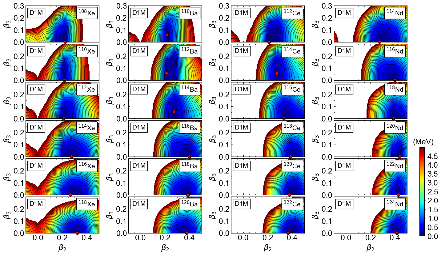
Figure 1: SCMF-PESs, as functions of the quadrupole $\beta_{2}$ and octupole $\beta_{3}$ deformations, for ^108-118Xe, ^110-120Ba, ^112-122Ce, and ^114-124Nd. The color code indicates the total HFB energies (in MeV) plotted up to 5 MeV with respect to the global minimum. The energy difference between neighboring contours is 0.2 MeV. For each nucleus, the global minimum is indicated by a red solid circle. Results have been obtained with the Gogny-D1M EDF.

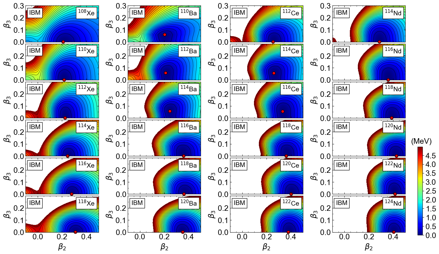
Figure 2: The same as in Fig. 1, but for the mapped IBM-PESs.

From a microscopic point of view, IBM bosons represent collective pairs of valence nucleons [76, 77, 78]. In principle, one should consider both neutron and proton bosons, which correspond to neutron-neutron and proton-proton pairs, respectively, within the framework of the proton-neutron IBM (IBM-2) [77]. However, in order to keep our approach as simple as possible, we have employed the simpler IBM-1 framework, which does not make a distinction between proton and neutron boson degrees of freedom.

Within the standard IBM framework, neutron-proton pairs are not included. In medium-heavy and heavy nuclei, to which the IBM has been mainly applied, neutrons and protons occupy different major oscillator shells and, therefore, the contribution of the neutron-proton coupling is expected to be negligible. On the other hand, for $N\approx Z$ nuclei in addition to the neutron-neutron and proton-proton pairs the neutron-proton pairs should be considered, since, in this case, both protons and neutrons can occupy similar orbits. However, this would require the introduction of additional isospin degrees of freedom in the IBM [79, 80]. This is probably the reason why the IBM has rarely been applied to $N\approx Z$ nuclei. For the same reason, the $sdf$-IBM framework employed in the present study does not consider the neutron-proton pairs.

The total number of bosons $n=n_{s}+n_{d}+n_{f}$ is equal to half the number of valence nucleons within the neutron and proton $N,Z=50-82$ major shells, and is conserved for a given nucleus. In the majority of the $sdf$-IBM phenomenology, certain truncation of the boson model space has been considered, that is, the maximum number of $f$ bosons $n_{f}^{\mathrm{max}}$ is limited to $n_{f}^{\mathrm{max}}=1$ or $n_{f}^{\mathrm{max}}=3$. In the present study, we do not make such an assumption, but allow $n_{f}$ to vary between zero and $n$.

The $sdf$-IBM Hamiltonian employed in the present study has the form [61, 63]:

$$\hat{H}=\epsilon_{d}\hat{n}_{d}+\epsilon_{f}\hat{n}_{f}+\kappa_{2}\hat{Q}_{2}\cdot\hat{Q}_{2}+\rho\hat{L}\cdot\hat{L}+\kappa_{3}\hat{Q}_{3}\cdot\hat{Q}_{3}.$$ (1)

The first (second) term on the right-hand side represents the number operator for the $d$ ($f$) bosons with $\epsilon_{d}$ ($\epsilon_{f}$), standing for the single $d$ ($f$) boson energy relative to the $s$ boson one. The third, fourth and fifth terms represent the quadrupole-quadrupole interaction, the rotational term, and the octupole-octupole interaction, respectively. The quadrupole $\hat{Q}_{2}$, angular momentum $\hat{L}$, and octupole $\hat{Q}_{3}$ operators read

$$\hat{Q}_{2}=s^{\dagger}\tilde{d}+d^{\dagger}\tilde{s}+\chi_{d}(d^{\dagger}\tilde{d})^{(2)}+\chi_{f}(f^{\dagger}\tilde{f})^{(2)}$$ (2a)

$$\hat{L}=\sqrt{10}(d^{\dagger}\tilde{d})^{(1)}+\sqrt{28}(f^{\dagger}\tilde{f})^{(1)}$$ (2b)

$$\hat{Q}_{3}=s^{\dagger}\tilde{f}+f^{\dagger}\tilde{s}+\chi_{3}(d^{\dagger}\tilde{f}+f^{\dagger}\tilde{d})^{(3)}.$$ (2c)

Note that the term proportional to $(d^{\dagger}\tilde{d})^{(1)}\cdot(f^{\dagger}\tilde{f})^{(1)}$ in the $\hat{L}\cdot\hat{L}$ term has been neglected [61]. Exception made of $\rho$, all the parameters of the $sdf$-IBM Hamiltonian are determined, for each nucleus, by mapping the SCMF-PES onto the corresponding IBM-PES [60, 61]. This requires the approximate equality $E_{\mathrm{HFB}}(\beta_{2},\beta_{3})\approx E_{\mathrm{IBM}}(\beta_{2},\beta_{3})$ to be satisfied in the neighborhood of the global minimum. The IBM-PES is defined as the expectation value of the $sdf$-IBM Hamiltonian in the boson condensate state [81] wave function $\ket{n,\beta_{2},\beta_{3}}$, i.e., $E_{\mathrm{IBM}}(\beta_{2},\beta_{3})=\bra{n,\beta_{2},\beta_{3}}\hat{H}\ket{n,\beta_{2},\beta_{3}}$, where

$$|n,\beta_{2},\beta_{3}\rangle=(n!)^{-1/2}(b_{c}^{\dagger})^{n}\ket{0}$$ (3a)

with

$$b_{c}^{\dagger}=(1+{\bar{\beta}_{2}}^{2}+{\bar{\beta}_{3}}^{2})^{-1/2}(s^{\dagger}+\bar{\beta}_{2}d_{0}^{\dagger}+\bar{\beta}_{3}f_{0}^{\dagger}).$$ (3b)

The ket $\ket{0}$ denotes the boson vacuum, or inert core. The doubly-magic nucleus ¹⁰⁰Sn is taken as the inert core in the present study, hence $n=(A-100)/2$ for a nucleus with mass $A$. The amplitudes $\bar{\beta}_{2}$ and $\bar{\beta}_{3}$ entering the definition of the boson condensate wave function are proportional to the $\beta_{2}$ and $\beta_{3}$ deformations of the fermionic space, $\bar{\beta}_{2}=C_{2}\beta_{2}$ and $\bar{\beta}_{3}=C_{3}\beta_{3}$ [81, 59, 60], with dimensionless proportionality constants $C_{2}$ and $C_{3}$. Their values are also determined by the mapping procedure, so that the location of the global minimum in the SCMF-PES is reproduced. Finally, the parameter $\rho$ is fixed [82] by equating the cranking moment of inertia obtained in the intrinsic frame of the IBM [83] at the global minimum to the corresponding Thouless-Valatin (TV) value [84] computed with the Gogny-HFB cranking method. For a more detailed description of the whole procedure the reader is referred to Ref. [61]. For the numerical diagonalization of the mapped Hamiltonian $\hat{H}$ (1), we use the computer code arbmodel [85].

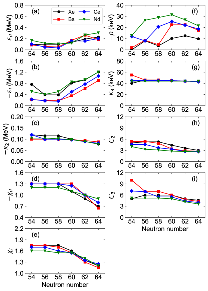
Figure 3: Strength parameters (a) $\epsilon_{d}$, (b) $\epsilon_{f}$, (c) $\kappa_{2}$, (d) $\chi_{d}$, (e) $\chi_{f}$, (f) $\rho$, and (g) $\kappa_{3}$, of the $sdf$-IBM Hamiltonian (1), and the coefficients (h) $C_{2}$ and (i) $C_{3}$. for the studied isotopic chains. For more details, see the main text.

III Potential energy surfaces

The Gogny-D1M SCMF-PESs obtained for the studied Xe, Ba, Ce, and Nd nuclei are depicted in Fig. 1. A shallow octupole-deformed minimum is observed for the $N\approx 56$ nuclei ¹¹⁰Ba, ¹¹²Ba, ¹¹⁴Ba, and ¹¹⁴Ce. On the other hand, the ground states of all the considered Xe and Nd nuclei are reflection-symmetric. Nevertheless, especially for ¹⁰⁸Xe, ¹¹⁰Xe and ¹¹²Xe the SCMF-PESs are rather soft along the $\beta_{3}$ direction. For $N\gg 56$, the octupole minimum disappears in all the isotopic chains while well quadrupole-deformed ground states emerge. The SCMF-PESs resulting from the Gogny-HFB calculations are qualitatively similar to the ones obtained from the constrained relativistic mean-field calculations based on the DD-PC1 EDF [51]. The major difference is that the latter predict $\beta_{3}^{\mathrm{min}}=0$ for ¹¹⁰Ba.

The mapped IBM-PESs are plotted in Fig. 2. They reproduce the overall features of the SCMF-PESs, such as the location of the global minimum and the softness along the $\beta_{3}$-direction. In comparison to the SCMF-PESs, the IBM ones are flat especially in regions corresponding to large $\beta_{2}$ and $\beta_{3}$ values that are far from the global minimum. This is a common feature within the IBM framework arising from the fact that the IBM consists of valence nucleon pairs in one major shell, while the SCMF model involves all nucleon degrees of freedom. For a detailed account of this problem, the reader is referred to Ref. [63].

The parameters for the Hamiltonian (1), determined by the mapping procedure, are shown in Fig. 3. Each parameter exhibits a weak dependence on the neutron number $N$ and, in some cases, is almost constant. For most of the parameters, there is no striking difference in their values and $N$-dependence for the considered isotopic chains. For the sake of simplicity, the parameters $\chi_{f}$ and $\chi_{3}$ are assumed to have the same magnitude $\chi_{3}=-\chi_{f}$, and only the $\chi_{f}$ value is plotted in panel (e).

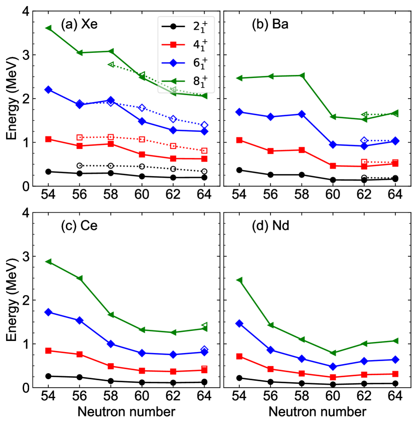
Figure 4: The low-energy excitation spectra of positive-parity ($\pi=+1$) even-spin yrast states obtained for ^108-118Xe, ^110-120Ba, ^112-122Ce, and ^114-124Nd are compared with the available experimental data [86]. Theoretical (experimental) values are represented by filled (open) symbols connected by solid (dotted) lines.

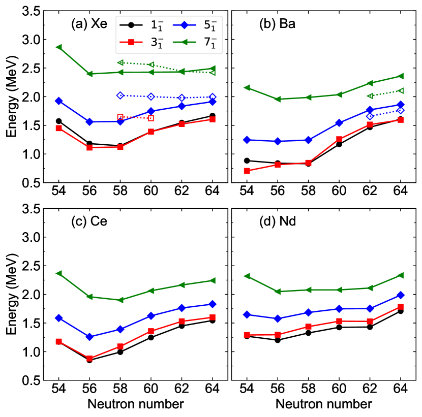
Figure 5: The same as in Fig. 4, but for the negative-parity ($\pi=-1$) odd-spin states.

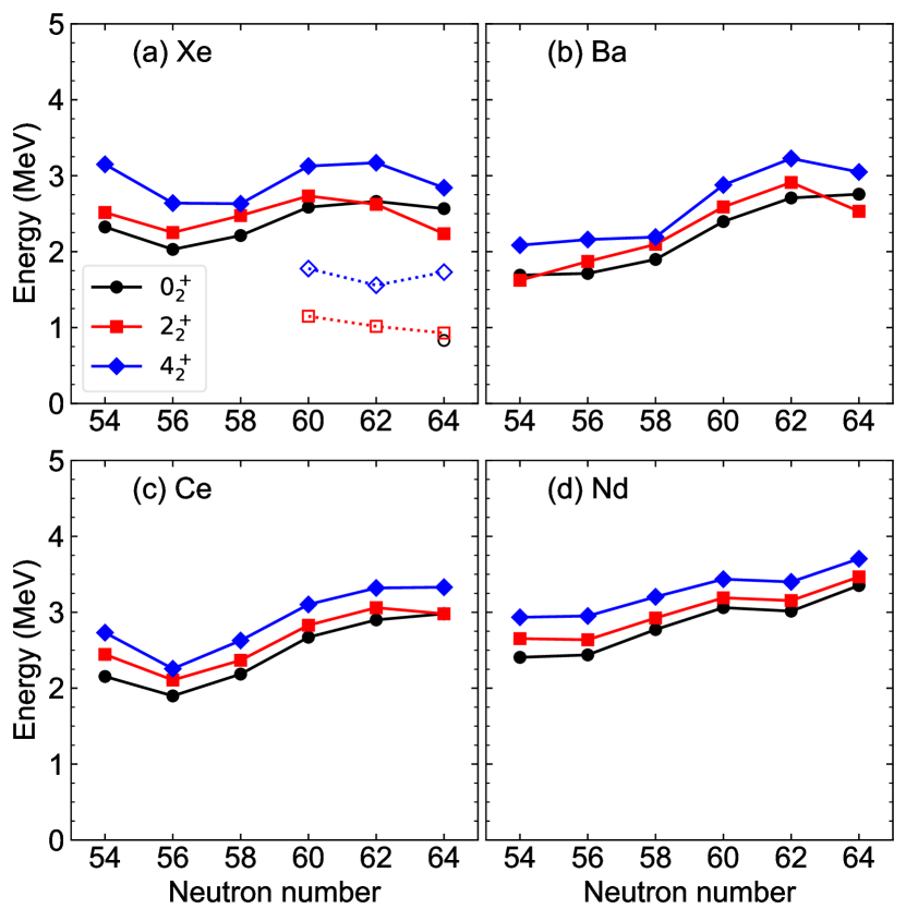
Figure 6: The same as in Fig. 4, but for the quasi-$\beta$ band states.

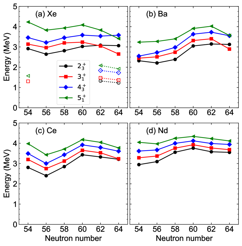
Figure 7: The same as in Fig. 4, but for the quasi-$\gamma$ band states.

Figure 8: The expectation values of the $f$-boson number operator $\braket{\hat{n_{f}}}$ in the IBM wave functions corresponding to the $K=0^{+}_{1}$(a) and $K=0^{-}_{1}$ (b) states, the quasi-$\beta$ (c) and quasi-$\gamma$ (d) bands of Xe isotopes.

IV Results for spectroscopic properties

IV.1 Excitation energies for yrast states

The low-energy excitation spectra corresponding to the $\pi=+1$ even-spin yrast states in ^108-118Xe, ^110-120Ba, ^112-122Ce, and ^114-124Nd are plotted in Fig. 4. As can be seen from the figure, the $\pi=+1$ excitation energies decrease with increasing neutron number. The calculated $\pi=+1$ ground-state ($K=0^{+}_{1}$) band for those Xe nuclei with $N\geqslant 60$ appear to be more compressed than the experimental ones. The $\pi=+1$ spectra for Ba and Ce nuclei with $N\geqslant 62$ agree reasonably well with the experiment. For Xe and Ba isotopes, the predicted excitation energies exhibit a pronounced decrease from $N=58$ to 60, suggesting the onset of a pronounced quadrupole collectivity. This correlates well with the features observed in the corresponding Gogny-D1M SCMF-PESs in Fig. 1. Note, that the SCMF-PESs become rather soft along the $\beta_{2}$-direction for $N\geqslant 60$.

The spectra corresponding to the $\pi=-1$ odd-spin yrast states are depicted in Fig. 5. The predicted excitation energies exhibit a weak dependence with neutron number, reaching a minimal value around $N=56$. This tendency reflects that for that neutron number the SCMF-PESs exhibit an octupole-deformed minimum or are notably soft along the $\beta_{3}$-direction (see Fig. 1). The mapped $sdf$-IBM predicts $\pi=-1$ levels lower in energy than the experimental ones. Similar results have been obtained in Ref. [51] for the odd-spin $\pi=-1$ band centered around $N=56$. However, the $\pi=-1$ excitation energies obtained in those calculations are higher than the present results.

IV.2 Excitation energies for non-yrast states

The excitation energies of the non-yrast states $0^{+}_{2}$, $2^{+}_{2}$, and $4^{+}_{2}$ are shown in Fig. 6. In most cases, these states are the lowest-spin members of the quasi-$\beta$ band, interconnected by strong $E2$ transitions. For ¹¹⁶Xe, ¹¹⁸Xe, ¹²⁰Ba and ¹²²Ce, the predicted quasi-$\beta$ band is comprised of the $0^{+}_{2}$, $2^{+}_{3}$, and $4^{+}_{3}$ states. This explains the inversion of the $0^{+}_{2}$ and $2^{+}_{2}$ levels in Fig. 6 for these particular nuclei. The predicted quasi-$\beta$ states exhibit a weak parabolic dependence as functions of $N$, with a minimum around $N=56$. The excitation energy of the band-head state $0^{+}_{2}$ is systematically high (above 2 MeV excitation from the ground state), overestimating the experimental values for ¹¹⁴Xe, ¹¹⁶Xe, and ¹¹⁸Xe by a factor of two. The mapped IBM procedure often yields excitation energies of non-yrast states higher than the experimental ones. The discrepancy suggest that some of the values obtained for the Hamiltonian parameters might not be reasonable. Specifically, for the quadrupole-quadrupole boson interaction strength we have obtained $\kappa_{2}\approx-0.1$ MeV (see Fig. 3(c)), while purely phenomenological IBM calculations (see, for example, [87] for ¹¹⁸Xe) usually employ a value for this parameter that is an order of magnitude smaller. In the mapped $sdf$-IBM framework, the large magnitude of the derived $\kappa_{2}$ parameter often leads to non-yrast $\pi=+1$ bands lying quite high in energy with respect to the ground-state band [64]. The calculations [88, 87] with the parameters fitted to experimental data, on the other hand, generally reproduced the observed quasi-$\beta$ and quasi-$\gamma$ bands quite nicely. The values of the derived IBM parameters, however, reflect the topology of the SCMF-PES. Many of the available EDFs yield SCMF-PESs with a steep valley along the $\beta_{2}$-direction around the global minimum. This often requires to choose IBM parameters quite different from those in phenomenological studies.

The predicted excitation energies for the $2^{+}_{3}$, $3^{+}_{1}$, $4^{+}_{3}$, and $5^{+}_{1}$ states are shown in Fig. 7. Those states are considered as members of the quasi-$\gamma$ band, exception made of ¹¹⁶Xe, ¹¹⁸Xe, ¹²⁰Ba, and ¹²²Ce for which the $2^{+}_{2}$ and $4^{+}_{2}$ are the states to be assigned as the even-$I$ members of the $\gamma$ band. As with the quasi-$\beta$ band, the predicted energies display a parabolic trend centered around $N=56$, whereas the band-head energy is too high with respect to the yrast band.

IV.3 $f$-boson content of the bands

We have analyzed the relevance of the octupole degree of freedom in the predicted bands. In particular, changes in the $f$-boson content in the bands with the neutron number can be considered as signatures of shape/phase transitions involving octupolarity. The expectation value of the $f$-boson number operator $\braket{\hat{n}_{f}}$ for states in the ground-state ($K=0^{+}_{1}$), lowest $\pi=-1$ ($K=0^{-}_{1}$), quasi-$\beta$, and quasi-$\gamma$ bands is plotted in Fig. 8. Results are shown for Xe isotopes as illustrative examples.

As seen from Fig. 8(a), for $I\leqslant 6^{+}$ the members of the ground-state band are dominated by the positive-parity $s$ and $d$ bosons, while the contribution from the negative-parity $f$ boson is minor ($\braket{\hat{n}_{f}}<1$). In the case of transitional nuclei with $N\leqslant 58$, the $f$-boson components start to dominate the higher-spin states with $I\geqslant 8^{+}$. The odd-$I$ states in the $K=0^{-}_{1}$ band for all the Xe nuclei have expectation values which are typically within the range $1<\braket{\hat{n}_{f}}<1.5$ and therefore can be interpreted as being made of one $f$ boson coupled to the $sd$ bosons space.

In Fig. 8(c), the structure of the quasi-$\beta$ band, which includes the $0^{+}_{2}$, $2^{+}_{2}$, and $4^{+}_{2}$ states, substantially differs from one nucleus to another. For the transitional nuclei with $56\leqslant N\leqslant 60$, the quasi-$\beta$ band is considered to be of double-octupole-phonon nature with $\braket{\hat{n}_{f}}\approx 2$. On the other hand, for well-quadrupole deformed nuclei with $N=62$ and $N=64$, the expectation value $\braket{\hat{n}_{f}}$ decreases and the contribution from the $f$ boson becomes less important. An irregularity is observed for $N=54$. However, in this case, the number of bosons is only $n=4$ and the IBM description can be expected to be worse than for nuclei with a larger number of bosons. Similar observations can be made for the quasi-$\gamma$ band (Fig. 8(d)), which is comprised of the $2^{+}_{3}$, $3^{+}_{1}$, $4^{+}_{3}$, and $5^{+}_{1}$ states.

Figure 9: Experimental and predicted band structures in ¹¹⁴Xe, ¹¹⁶Xe, and ¹¹⁸Xe.

IV.4 Band structure of individual nuclei

Experimental information is available for ¹¹⁴Xe, ¹¹⁶Xe, and ¹¹⁸Xe nuclei. This allows to assess the quality of the model description. The partial level schemes predicted for ¹¹⁴Xe, ¹¹⁶Xe, and ¹¹⁸Xe are compared in Fig. 9 with the available experimental data [86].

The nucleus ¹¹⁴Xe represents a transitional system between the nearly spherical and the strongly quadrupole deformed shapes (see, Fig. 1). As can be seen from Fig. 9(a) the mapped $sdf$-IBM calculations reproduce the lowest $\pi=\pm 1$ ($K=0^{\pm}_{1}$) bands reasonably well. While the observed $\pi=+1$ spectra look harmonic, the theoretical ones exhibit rotational SU(3) features: the ground-state band resembles a rotational band with a moment of inertia larger than the experimental one; both the quasi-$\beta$ and quasi-$\gamma$ bands are high in energy with respect to the ground-state band; the moments of inertia for the ground-state, quasi-$\beta$, and quasi-$\gamma$ bands are almost equal to each other. Both empirically and theoretically, the $\pi=-1$ even-$I$ states are found above 2 MeV excitation from the ground state.

Within the Gogny-HFB framework ¹¹⁶Xe displays a large quadrupole deformation (see Fig. 1). The experimental band structure of ¹¹⁶Xe is similar to the band structure of ¹¹⁴Xe. The mapped $sdf$-IBM reproduces the ground-state and lowest $\pi=-1$ ($K=0^{-}_{1}$) bands, though they are stretched compared to the experimental bands. The band-heads of the quasi-$\beta$ and quasi-$\gamma$ bands have an excitation energy around 2.5 MeV. In comparison with ¹¹⁴Xe, the predicted quasi-$\beta$ band looks more irregular, as seen, for example, from the large energy gap between the $4^{+}_{3}$ and $6^{+}_{4}$ levels. This is a consequence of the strong level repulsion between low-spin states due to a considerable amount of shape mixing. From the experimental point of view, the band built on the $2^{+}_{3}$ state is tentatively assigned to be quasi-$\gamma$ band. Such a band exhibits the staggering pattern $(2^{+}_{\gamma},3^{+}_{\gamma}),(4^{+}_{\gamma},5^{+}_{\gamma}),\ldots$ and resembles the level structure predicted in the rigid-triaxial rotor model [89]. In contrast, the quasi-$\gamma$ band obtained in the present calculation shows the staggering pattern $2^{+}_{\gamma},(3^{+}_{\gamma},4^{+}_{\gamma}),(5^{+}_{\gamma},6^{+}_{\gamma}),\ldots$ characteristic of the $\gamma$-unstable-rotor picture [90].

Figure 9(c) displays the results obtained for ¹¹⁸Xe. The $K=0^{\pm}_{1}$ bands predicted within the mapped $sdf$-IBM approach agree well with the experimental data. The $0^{+}_{2}$ state and the band built on it are known experimentally, with a band-head energy below 1 MeV. The quasi-$\gamma$ band with the staggering pattern, $2^{+}_{\gamma},(3^{+}_{\gamma},4^{+}_{\gamma}),(5^{+}_{\gamma},6^{+}_{\gamma}),\ldots$ is also known experimentally . As can be seen, the quasi-$\beta$ and quasi-$\gamma$ bands are much higher than their experimental counterparts. Nevertheless, overall features of the bands, such as the moments of inertia and energy splitting members of the bands, agree well with the experiment. Note, that the band-head energy of the predicted quasi-$\beta$ band is slightly lower than that of the quasi-$\gamma$ band.

At this point it is worth to make a few remarks on some of the features of the predicted spectra shown in Fig. 9. First, the moments of inertia for the predicted ground-state bands at low spin are systematically larger than the experimental ones, with too low $2^{+}_{1}$ excitation energies and $E(4^{+}_{1})/E(2^{+}_{1})$ ratios close to the rotor limit value $3.33$. The responsible for this behavior is the TV moment of inertia obtained in the cranking calculation with the Gogny force. The cranking rotational band corresponds to a very good rotor and the moment of inertia is roughly a factor of two larger than the experimental data. As the moment of inertia is inversely proportional to the square of the pairing gap, the disagreement is probably a consequence of the missing proton-neutron pairing present in $N\approx Z$ nuclei and not considered in neither the cranking calculation nor the $sdf$-IBM Hamiltonian. Second, for the three Xe nuclei one observes almost degenerated $1^{-}_{1}$ and $3^{-}_{1}$ energy levels corresponding to the $K=0^{-}_{1}$ band with the $3^{-}_{1}$ slightly below the $1^{-}_{1}$, which is at variance with the empirical trend of negative parity rotational bands. Such irregularity may suggest that there is strong configuration mixing in the low-spin $\pi=-1$ states. It could also reflect the lack of the dipole $p$ boson degree of freedom with spin and parity $1^{-}$ in our model space. Its inclusion could allow a more accurate description of the low-spin part of the $0^{-}_{1}$ band.

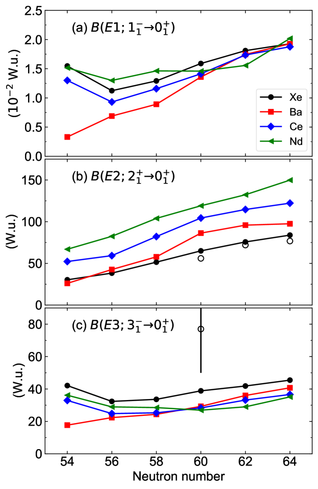
Figure 10: The calculated $B(E1;1^{-}_{1}\to 0^{+}_{1})$ (a), $B(E2;2^{+}_{1}\to 0^{+}_{1})$ (c), and $B(E3;3^{-}_{1}\to 0^{+}_{1})$ (e) reduced transition probabilities in Weisskopf units (W.u.), represented by the solid symbols connected by lines. Experimental data for the Xe nuclei are taken from [86, 12, 16, 87], and are represented by the open symbols. Note that the error bars for the experimental $B(E2)$ rates of ^114,116,118Xe are not shown, as they are smaller than the marker size.

IV.5 Electric transition rates

The electric dipole ($E1$), quadrupole ($E2$), and octupole $(E3)$ transition probabilities are computed using the corresponding operators defined as $\hat{T}(E1)=e_{1}(d^{\dagger}\tilde{f}+f^{\dagger}\tilde{d})^{(1)}$, $\hat{T}(E2)=e_{2}\hat{Q}_{2}$, and $\hat{T}(E3)=e_{3}\hat{Q}_{3}$, respectively. The operators $\hat{Q}_{2}$ and $\hat{Q}_{3}$ have the same forms and parameters as those in Eqs. (2a) and (2c). The boson effective $E1$ and $E3$ charges $e_{1}=0.01$ $e\,$b^1/2 and $e_{3}=0.12$ $e\,$b^3/2 are adopted from our previous study on the neutron-rich Ba region [59, 64]. The $E2$ boson charge $e_{2}=0.107$ $e\,$b is fixed so that the experimental $B(E2;2^{+}_{1}\to 0^{+}_{1})$ transition rates for Xe nuclei [86, 12, 87] are reproduced reasonably well. The computed $B(E1;1^{-}_{1}\to 0^{+}_{1})$, $B(E2;2^{+}_{1}\to 0^{+}_{1})$, and $B(E3;3^{-}_{1}\to 0^{+}_{1})$ transition probabilities are shown in Fig. 10. The available experimental data are the $B(E2)$ transition rates for ¹¹⁴Xe [12], ¹¹⁶Xe [12], and ¹¹⁸Xe [87], and the $B(E3)$ value for ¹¹⁴Xe [16].

The $B(E1)$ transition probabilities obtained for Xe, Ce, and Nd nuclei are plotted in Fig. 10(a). They exhibit a parabolic dependence on $N$ with a minimum around $N=56$. This trend correlates with the systematic of the $E(1^{-}_{1})$ energy (see Fig. 5). A similar trend was obtained for Xe isotopes in Ref. [51]. However, one should keep in mind that the $E1$ properties may have a strong component determined by noncollective (single-particle) degrees of freedom, which are by construction not included in the configuration space of the $sdf$-IBM. Thus the mapped IBM framework, in its current version, does not provide an accurate description of the $E1$ transitions. The $B(E2)$ rates in Fig. 10(b) increase monotonously with $N$, which confirms the increasing quadrupole collectivity. The $2^{+}_{1}$ excitation energy also becomes lower, as one approaches the middle of the neutron major shell $N=66$ (see Fig. 4).

In the case of nuclei with pronounced octupole deformation effects, the $B(E3;3^{-}_{1}\to 0^{+}_{1})$ transition probabilities are expected to be large. As can be see from Fig. 10(c), the predicted $B(E3)$ values do not show this pattern. To take into account the empirical isotopic dependence of the $B(E3;3^{-}_{1}\to 0^{+}_{1})$ rate, in earlier studies [63, 64] we assumed the boson effective $E3$ charge to have a certain boson-number dependence. In the present study, however, we have used the constant $E3$ charge $e_{3}=0.12$ $e\,$b^2/3, mainly due to the lack of $B(E3)$ data. The present calculations underestimate the large experimental $B(E3;3^{-}_{1}\to 0^{+}_{1})$ value for ¹¹⁴Xe ($77\pm 27$ W.u.) [16]. The data, however, also has a large error bar.

Table 1: The $B(E1)$, $B(E2)$, and $B(E3)$ transition probabilities (in W.u.) obtained for ¹¹²Xe, ¹¹⁴Xe, ¹¹⁶Xe and ¹¹⁸Xe are compared with experimental data from Refs. [86, 91, 12, 15, 16, 87].

	$E\lambda$	$I_{i}$	$I_{f}$	Expt.	IBM
112Xe	$E1$	$5^{-}_{1}$	$4^{+}_{1}$	$(1.0\pm 0.3)\times 10^{-4}$	$5.4\times 10^{-3}$
		$7^{-}_{1}$	$6^{+}_{1}$	$(6\pm 2)\times 10^{-5}$	$7.4\times 10^{-3}$
114Xe	$E1$	$3^{-}_{1}$	$4^{+}_{1}$	$(7.4\pm 2.1)\times 10^{-5}$	$2.4\times 10^{-5}$
			$2^{+}_{1}$	$(2.0\pm 0.5)\times 10^{-5}$	$3.6\times 10^{-3}$
		$5^{-}_{1}$	$6^{+}_{1}$	$(1.6\pm 0.2)\times 10^{-4}$	$2.0\times 10^{-6}$
	$E2$	$2^{+}_{1}$	$0^{+}_{1}$	56$\pm 4$	65
		$4^{+}_{1}$	$2^{+}_{1}$	56$\pm 3$	90
		$6^{+}_{1}$	$4^{+}_{1}$	43$\pm 6$	93
		$5^{-}_{1}$	$3^{-}_{1}$	94$\pm 11$	58
		$7^{-}_{1}$	$5^{-}_{1}$	69$\pm 15$	63
	$E3$	$3^{-}_{1}$	$0^{+}_{1}$	77$\pm 27$	39
		$5^{-}_{1}$	$2^{+}_{1}$	68$\pm 17$	59
116Xe	$E1$	$7^{-}_{1}$	$6^{+}_{1}$	$(1.4\pm 0.6)\times 10^{-4}$	$8.2\times 10^{-3}$
		$9^{-}_{1}$	$8^{+}_{1}$	$(9.4\pm 1.2)\times 10^{-5}$	$1.1\times 10^{-2}$
	$E2$	$2^{+}_{1}$	$0^{+}_{1}$	72$\pm 3$	76
		$4^{+}_{1}$	$2^{+}_{1}$	127$\pm 5$	106
		$6^{+}_{1}$	$4^{+}_{1}$	113$\pm 10$	112
		$8^{+}_{1}$	$6^{+}_{1}$	100$\pm 12$	108
		$10^{+}_{1}$	$8^{+}_{1}$	113$\pm 21$	97
		$7^{-}_{1}$	$5^{-}_{1}$	82$\pm 44$	72
		$9^{-}_{1}$	$7^{-}_{1}$	90$\pm 15$	79
		$11^{-}_{1}$	$9^{-}_{1}$	86$\pm 10$	79
118Xe	$E1$	$7^{-}_{1}$	$6^{+}_{1}$	$(2.3\pm 0.1)\times 10^{-4}$	$8.2\times 10^{-3}$
		$9^{-}_{1}$	$8^{+}_{1}$	$(2.2\pm 0.1)\times 10^{-4}$	$1.1\times 10^{-2}$
		$11^{-}_{1}$	$10^{+}_{1}$	$(1.2\pm 0.3)\times 10^{-4}$	$1.3\times 10^{-2}$
	$E2$	$2^{+}_{1}$	$0^{+}_{1}$	76.8$\pm 1.1$	84
		$4^{+}_{1}$	$2^{+}_{1}$	118$\pm 2$	119
		$6^{+}_{1}$	$4^{+}_{1}$	156${}^{+7}_{-6}$	127
		$8^{+}_{1}$	$6^{+}_{1}$	143${}^{+17}_{-13}$	125

Table 1 lists the $B(E\lambda)$ values for ¹¹²Xe, ¹¹⁴Xe, ¹¹⁶Xe, and ¹¹⁸Xe, for which experimental data are available [86, 91, 12, 16, 87]. For the $B(E2)$ rates, only the data for inband transitions in the lowest-energy $\pi=\pm 1$ bands are known. The calculations account reasonably well for the $B(E2;I\to{I-2})$ values in ^116,118Xe. For ¹¹⁴Xe, the mapped IBM overestimates these inband $E2$ transitions, which suggests a much stronger quadrupole collectivity than expected experimentally. For completeness, some $B(E1)$ rates are also included in the table.

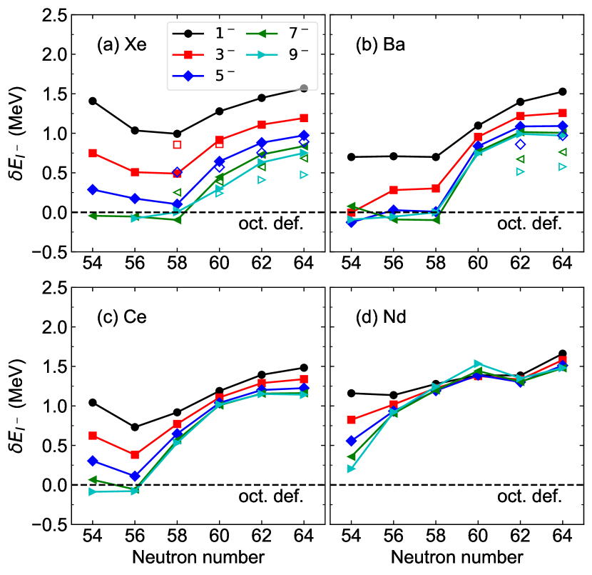
Figure 11: The energy displacement $\delta{E_{I^{-}}}$ (4) is plotted as a function of the neutron number. Theoretical values are connected by lines. Experimental values [86] for the $I^{\pi}=3^{-}$, $5^{-}$, $7^{-}$, and $9^{-}$ yrast states are represented by open squares, diamonds, and left- and right-pointing triangles, respectively. A broken horizontal line in each panel stands for the limit of stable octupole deformation $\delta{E_{I^{-}}}=0$.

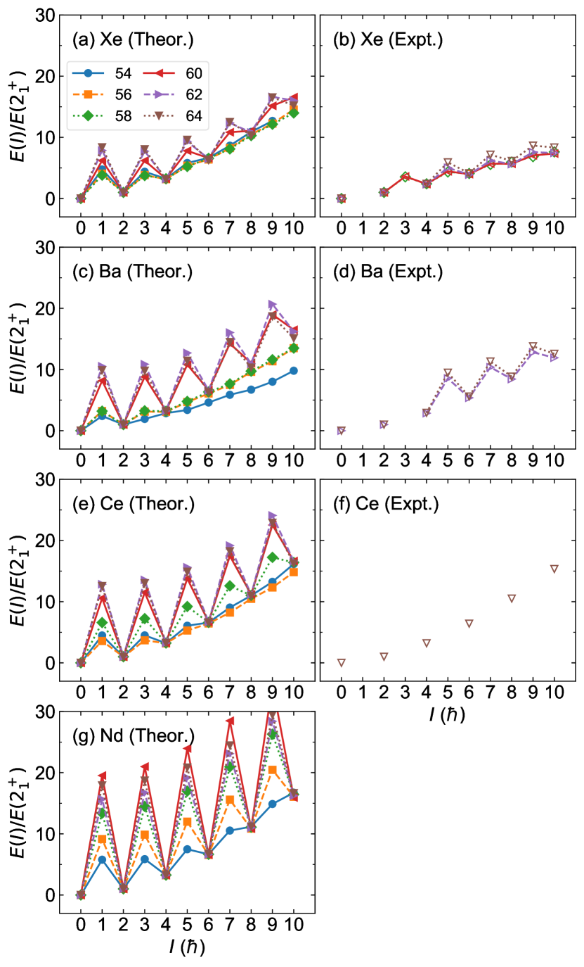
Figure 12: The energy ratio $E(I^{\pi})/E(2^{+}_{1})$ is plotted as a function of spin $I^{\pi}$, with $\pi=+1$ for even-$I$ and $\pi=-1$ for odd-$I$ yrast states. The available experimental data for the Xe, Ba, and Ce isotopes are taken from [86].

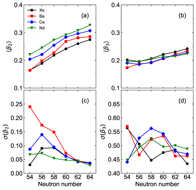
Figure 13: Effective quadrupole (a) and octupole (b) deformations $\braket{\beta_{\lambda}}$ and fluctuations $\sigma(\beta_{\lambda})$ in the $\beta_{2}$ (c) and $\beta_{3}$ (d) deformations. For more details, see the main text.

V Signatures of octupole shape phase transition

V.1 Possible alternating-parity band structure

In order to distinguish whether the members of $\pi=-1$ rotational bands are octupole-deformed or octupole vibrational states, it is convenient to analyze the energy displacement, defined by

$$\delta{E_{I^{-}}}=E_{I^{-}}-\frac{E_{(I+1)^{+}}+E_{(I-1)^{+}}}{2},$$ (4)

where $E_{I^{-}}$ and $E_{(I\pm 1)^{+}}$ represent the excitation energies of the $\pi=-1$ odd-spin and $\pi=+1$ even-spin yrast states, respectively. If the two lowest bands with opposite parity share an octupole deformed band-head they form an alternating-parity doublet and the quantity $\delta{E_{I^{-}}}$ should be equal to zero. The deviation from the limit $\delta{E_{I^{-}}}=0$, implies that the states generating the $\pi=\pm 1$ bands are different in nature, and therefore the $\pi=-1$ state has an octupole vibrational character.

The $\delta{E_{I^{-}}}$ values are displayed in Fig. 11. This quantity is close to zero for Xe, Ba, and Ce nuclei with $54\leqslant N\leqslant 58$, especially for higher-spin states. One observes a pronounced increase of $\delta{E_{I^{-}}}$ from $N=58$ to 60 in the Ba and Xe isotopes and from $N=56$ to 58 in the Ce isotopes. The deviation from the limit ($\delta{E_{I^{-}}}=0$) becomes more significant for larger neutron numbers. Note, that for Xe and Ba isotopes, the $\delta{E_{I^{-}}}$ values agree well with the experimental ones [86].

We have also examined the energy ratio $E(I^{\pi})/E(2^{+}_{1})$, with $\pi=+1$ for even-$I$ and $\pi=-1$ for odd-$I$ yrast states. For the ideal alternating-parity rotational band the ratio would depend quadratically on the spin $I$. If the $\pi=\pm 1$ yrast bands are decoupled, as in the case of octupole vibrational states, the ratio is expected to show an odd-even-spin staggering. As can be seen from Fig. 12, the energy ratios for the Xe, Ba and Ce isotopes with $N<60$ increase quadratically with $I$. On the other hand, a pronounced odd-even-spin staggering occurs for $N\geqslant 60$. The staggering is much more pronounced for heavier-$Z$ isotopes. These results confirm that octupole correlations are enhanced around $N=56$ and $Z=56$.

V.2 Quadrupole and octupole shape invariants

We consider shape invariants [92, 93] computed using the $E2$ and $E3$ matrix elements as another signature of shape/phase transitions. The relevant shape invariants are defined as

$$q_{2}^{(\lambda)}=\sum_{i} (-1)^{I}\braket{0^{+}_{1}}{\hat{T}(E\lambda)}{I^{\pi}_{i}}\braket{I^{\pi}_{i}}{\hat{T}(E\lambda)}{0^{+}_{1}}$$ (5)

$$q_{4}^{(\lambda)}=\sum_{i,j,k} \braket{0^{+}_{1}}{\hat{T}(E\lambda)}{I^{\pi}_{i}}\braket{I^{\pi}_{i}}{\hat{T}(E\lambda)}{0^{+}_{j}}$$

$$\times\braket{0^{+}_{j}}{\hat{T}(E\lambda)}{I^{\pi}_{k}}\braket{I^{\pi}_{k}}{\hat{T}(E\lambda)}{0^{+}_{1}}$$ (6)

where $\ket{0^{+}_{1}}$ is the $sdf$-IBM ground state, $\braket{}{(\cdots)}{}$ represents the reduced $E2$ ($E3$) matrix element and $I^{\pi}=2^{+}$ ($3^{-}$) for $\lambda=2$ ($\lambda=3$). The sums in Eqs. (5) and (V.2) include up to ten lowest $0^{+}$, $2^{+}$, and $3^{-}$ states. The effective quadrupole and octupole deformations

$$\braket{\beta_{\lambda}}=\frac{4\pi}{3eZR_{0}^{\lambda}}\sqrt{q_{2}^{(\lambda)}}$$ (7)

as well as the fluctuations [93]

$$\sigma(\beta_{\lambda})=q_{4}^{(\lambda)}/(q_{2}^{(\lambda)})^{2}-1,$$ (8)

which measure the softness along the $\beta_{\lambda}$-directions are shown in Fig. 13.

The steady increase of $\braket{\beta_{2}}$ in Fig. 13(a), corroborates the increasing quadrupole collectivity along the considered isotopic chains. In contrast, the $\braket{\beta_{3}}$ values, in Fig. 13(b), change much less with $N$. The fluctuations $\sigma(\beta_{2})$, in Fig. 13(c), appear to reach a maximum around $N=56$, and show a notable decrease from $N=56$ toward $N=60$. Note, that the corresponding SCMF-PESs become more rigid along the $\beta_{2}$-direction from $N=56$ on, and a more distinct prolate minimum appears (see Fig. 1). This result is also consistent with the behavior of the predicted $\pi=+1$ energy spectra, which suggest the onset of strongly quadrupole deformed shapes at $N\approx 60$ (see Fig. 4). As seen in Fig. 13(d), the fluctuations $\sigma(\beta_{3})$ are systematically larger in magnitude than $\sigma(\beta_{2})$. The $\sigma(\beta_{3})$ values also exhibit a significant variation for $54\leqslant N\leqslant 62$. The behavior of the $\sigma(\beta_{3})$ fluctuations reflect a considerable degree of octupole mixing and an enhanced octupole collectivity.

VI Summary

The quadrupole-octupole coupling in the low-lying states of neutron-deficient Xe, Ba, Ce, and Nd nuclei has been studied within the mapped $sdf$-IBM framework. The strength parameters for the $sdf$-IBM Hamiltonian have been obtained via the mapping of the (microscopic) axially-symmetric $(\beta_{2},\beta_{3})$-PESs, obtained from constrained Gogny-D1M HFB calculations, onto the expectation value of the IBM Hamiltonian in the condensate state of the $s$, $d$, and $f$ bosons. Excitation spectra and electric transition probabilities have been obtained by the diagonalization of the mapped Hamiltonian.

The Gogny-D1M SCMF-PESs for nuclei near the neutron octupole “magic number” $N=56$ are notably soft along the $\beta_{3}$-direction. An octupole-deformed mean-field ground state has been obtained for ¹¹⁰Ba, ¹¹²Ba, ¹¹⁴Ba and ¹¹⁴Ce. Beyond the HFB level, the systematic of the properties of the positive parity states points towards an increased quadrupole collectivity with increasing neutron number. A notable change is found in Xe and Ba isotopes with $N=58$ and 60. The negative parity yrast states exhibit a parabolic behavior as functions of $N$, with a minimum around $N=56$. Moreover, the predicted $\pi=\pm 1$ yrast bands form an approximate alternating-parity doublet for most of the Xe isotopes as well as Ba and Ce nuclei in the vicinity of $N=56$. Another signature of octupole correlations can be associated with the large fluctuations of the effective $\beta_{3}$ deformation around $N=56$.

We have further assessed the predictive power of the mapped $sdf$-IBM to describe spectroscopic properties in the $N\approx Z$ mass region. The excitation energies of the $\pi=\pm 1$ yrast bands agree reasonably well with the available experimental data for Xe and Ba nuclei. However, non-yrast $\pi=+1$ bands have been predicted much higher in energy than the experimental ones. This indicates that certain extensions of the model are required to improve the description of non-yrast bands in regions of the nuclear chart where octupolarity plays a role. A reasonable approach to address this problem is to identify whether the deficiency in the model description of the non-yrast $\pi=+1$ bands is due to the deficiencies of the chosen EDF for the mass region under study, or that the employed $sdf$-IBM Hamiltonian lacks important degrees of freedom, or a combination of the two. Work along these lines is in progress and will be reported elsewhere.