Decays of the Heavy Top and New Insights on $\epsilon_{K}$ in a
one-VLQ Minimal Solution to the CKM Unitarity Problem

Francisco J. Botella ^a,, G. C. Branco ^b,, M. N. Rebelo ^b,, J.I. Silva-Marcos ^b, and José Filipe Bastos ^{b, a} Departament de Física Teòrica and IFIC,

Universitat de València-CSIC, E-46100 Burjassot, Spain.

^bCentro de Física Teórica de Partículas, CFTP,

Departamento de Física,

Instituto Superior Técnico, Universidade de Lisboa,

Avenida Rovisco Pais nr. 1, 1049-001 Lisboa, Portugal

                               PACS numbers : 12.10.Kt, 12.15.Ff, 14.65.Jk

We propose a minimal extension of the Standard Model where an up-type vector-like quark, denoted $T$, is introduced and provides a simple solution to the CKM unitarity problem. We adopt the Botella-Chau parametrization in order to extract the $4\times 3$ quark mixing matrix which contains the three angles of the $3\times 3$ CKM matrix plus three new angles denoted $\theta_{14}$, $\theta_{24}$, $\theta_{34}$. It is assumed that the mixing of $T$ with standard quarks is dominated by $\theta_{14}$. Imposing a recently derived, and much more restrictive, upper-bound on the New Physics contributions to $\epsilon_{K}$, we find, in the limit of exact $\theta_{14}$ dominance where the other extra angles vanish, that $\epsilon_{K}^{\text{NP}}$ is too large. However, if one relaxes the exact $\theta_{14}$ dominance limit, there exists a parameter region, where one may obtain $\epsilon_{K}^{\text{NP}}$ in agreement with experiment while maintaining the novel pattern of $T$ decays with the heavy quark decaying predominantly to the light quarks $d$ and $u$. We also find a reduction in the decay rate of $K_{L}\rightarrow\pi^{0}\nu\overline{\nu}$.

1 Introduction

The normalisation of the first row of $V^{CKM}$ provides one of the most stringent tests of $3\times 3$ unitarity of the quark mixing matrix of the Standard Model (SM). This results from the fact that the elements $|V_{ud}|$ and $|V_{us}|$ are measured with high accuracy and $|V_{ub}|$ is known to be very small. Recently, new theoretical calculations [1] – [9] of $V_{ud}$ and $V_{us}$ indicate that one may have $\left|V_{ud}\right|^{2}+\left|V_{us}\right|^{2}+\left|V_{ub}\right|^{2}<1$, thus implying a violation of $3\times 3$ unitarity. If confirmed, this would be a major result, providing evidence for New Physics (NP) beyond the SM.

It has been pointed out that one of the simplest extensions of the SM which can account for this NP, consists of the addition of either one down-type [10] or one up-type [11] vector-like quark (VLQ) isosinglet. In [12, 13] both of these possibilities were explored, as well as scenarios with other VLQ representations. In the case of a down-type VLQ isosinglet the CKM matrix consists of the first $3$ rows of a unitary $4\times 4$ matrix, while in the case of an up-type VLQ isosinglet, it consists of the first $3$ columns of a $4\times 4$ unitary matrix. In both cases, the parameter space is very large, involving six mixing angles and three CP violating phases. There are some common features in all models with VLQs, such as the appearance of Flavour-Changing-Neutral-Currents (FCNC) at tree level [14] – [23]. This is a clear violation of the dogma which states that no FCNC should exist at tree level. It should be stressed that models with VLQs predict the appearance of these dangerous currents, but provide a natural mechanism for their suppression. Models with VLQs have a rich phenomenology due to the large enhancement of the parameter space.

In this paper, we propose a specific up-type VLQ isosinglet model which solves the unitarity problem of the first row of $V^{CKM}$ and makes some striking predictions for the dominant decays of the heavy top quark $T$ and for the pattern of NP contributions for meson mixings. We adopt the Botella-Chau [23] parametrization where the new angles are denoted $\theta_{14}$, $\theta_{24}$ and $\theta_{34}$, and assume that $s_{14}\equiv\sin(\theta_{14})$ is the dominant new contribution. In the exact $s_{14}$ dominance limit, when $s_{24}=s_{34}=0$, the model predicts:

i) No tree level contributions to $D^{0}-\overline{D}^{0}$ mixing.

ii) The NP contributions to $B_{d}^{0}-\overline{B}_{d}^{0}$ and $B_{s}^{0}-\overline{B}_{s}^{0}$ mixings are negligible, when compared to the SM contributions.

iii) The new quark $T$ decays predominantly to the light quarks $d$ and $u$, contrary to the usual wisdom.

iv) There are important restrictions arising from NP contributions to $\epsilon_{K}$, specially taking into account the recent results [24] in constraining the allowed range for NP contributions to $\epsilon_{K}$. In particular, it was shown that it is no longer allowed to have a NP contribution to $\epsilon_{K}$ of the same size as the SM contribution. In this paper we show that the exact $s_{14}$ dominance limit is excluded since it leads to a too large contribution to $\epsilon_{K}$. However, we later show that the $s_{14}$ dominance is viable if we allow for small but non-vanishing values for $s_{24}$ and $s_{34}$. The introduction of small but non-vanishing values for $s_{24}$ and $s_{34}$ avoids the conflict with $\epsilon_{K}$ while at the same time maintaining the distinctive features of the $s_{14}$ limit.

2 The $s_{14}$ dominance hypothesis: a minimal implementation with one up-type VLQ.

We consider the SM with the minimal addition of one up-type ($Q=+2/3$) isosinglet VLQ, denoted by $U_{L}^{0}$ and $U_{R}^{0}$.

2.1 Framework: a minimal extension of the SM with one up-type VLQ

The relevant part of the Lagrangian, in the flavour basis, contains the Yukawa couplings and gauge invariant mass terms for the quarks:

$$-\mathcal{L}_{Y}=Y_{u}^{ij}\ \overline{Q}_{Li}^{0}\ \tilde{\phi}\ u_{Rj}^{0}+\overline{Y}^{i}\ \overline{Q}_{Li}^{0}\ \tilde{\phi}\ U_{R}^{0}+\overline{M}^{i}\ \overline{U}_{L}^{0}\ u_{Ri}^{0}+M\ \overline{U}_{L}^{0}\ U_{R}^{0}+Y^{ij}_{d}\ \overline{Q}_{Li}^{0}\ \phi\ d_{Rj}^{0}+h.c,$$ (1)

where $Y_{u,d}$ are the SM up and down quark Yukawa couplings, $\phi$ denotes the Higgs doublet ($\tilde{\phi}=\epsilon\,\phi^{*}$), $Q_{Li}^{0}=\left(u_{Li}^{0}\,\,d_{Li}^{0}\right)^{T}$ are the SM quark doublets and $u_{Ri}^{0},d_{Ri}^{0}$ ($i,j=1,2,3$) the up- and down-type SM right-handed quark singlets. Here, the $\overline{Y}^{i}$ represent the Yukawa couplings to the extra right-handed field $U_{R}^{0}$, while $\overline{M}$ and $M$ correspond, at this stage to bare mass terms. The right-handed VLQ field $U_{R}^{0}$ is, a priori, indistinguishable from the SM fermion singlets $u_{Ri}^{0}$, since it possess the same quantum numbers.

After the spontaneous breakdown of the electroweak gauge symmetry, the terms in Eq. (1) give rise to a $3\times 3$ mass matrix $m=\frac{v}{\sqrt{2}}\,Y_{u}$ and to a $3\times 1$ mass matrix $\overline{m}=\frac{v}{\sqrt{2}}\,\overline{Y}$ for the up-type quarks, with $v\simeq 246$ GeV. Together with $\overline{M}$ and $M$, they make up the full $4\times 4$ mass matrix,

$$\mathcal{M}_{u}=\left(\begin{array}[]{cc}m&\overline{m}\\ \overline{M}&M\end{array}\right)$$ (2)

One is allowed, without loss of generality, to work in a weak basis (WB) where the $3\times 3$ down-quark mass matrix $M_{d}=\frac{v}{\sqrt{2}}\,Y_{d}$ is diagonal, and in what follows we take $M_{d}=D_{d}=\mbox{diag}(m_{d},m_{s},m_{b})$.

The matrix $\mathcal{M}_{u}$ can be diagonalized by a bi-unitary transformation

$$\mathcal{V}^{\dagger}\ \mathcal{M}_{u}\ \mathcal{W}=\mathcal{D}_{u}$$ (3)

with $\mathcal{D}_{u}=\mbox{diag}(m_{u},m_{c},m_{t},m_{T})$, where $m_{T}$ is the mass of the heavy up-type quark $T$. The unitary rotations $\mathcal{V},\mathcal{W}$ relate the flavour basis to the physical basis.

When one transforms the quark field from the flavour to the physical basis, the charged current part of the Lagrangian becomes

$$\mathcal{L}_{W}=-{\frac{g}{\sqrt{2}}}\overline{u}_{Li}^{0}\left(\gamma^{\mu}W_{\mu}^{+}\right)d_{Li}^{0}=-{\frac{g}{\sqrt{2}}}\overline{u}_{L\alpha}\left(\gamma^{\mu}W_{\mu}^{+}\right)\left(\mathcal{V}^{\dagger}\right)^{\alpha i}d_{Li}$$ (4)

where the $u_{L}$ and $d_{L}$ are now in the physical basis. Notice that the down quark mass matrix is already diagonal. Thus, we find that the charged current quark mixing $\mathcal{V}^{CKM}$ corresponds to the $4\times 3$ block of the matrix $\mathcal{V}^{\dagger}$ specified in Eq. (3)

$$\mathcal{V}^{CKM}=\left(\mathcal{V}^{\dagger}\right)^{(4\times 3)}$$ (5)

The couplings to the $Z$ boson can be written as

$$\small\mathcal{L}_{Z}={\frac{g}{c_{W}}}Z_{\mu}\left[\frac{1}{2}\left(\overline{u}_{L}F^{u}\gamma^{\mu}u_{L}-\overline{d}_{L}F^{d}\gamma^{\mu}d_{L}\right)-s^{2}_{W}\left(\frac{2}{3}\overline{u}\gamma^{\mu}u-\frac{1}{3}\overline{d}\gamma^{\mu}d\right)\right]$$ (6)

with $F^{d}=\left(\mathcal{V}^{CKM}\right)^{\dagger}\mathcal{V}^{CKM}$ and $F^{u}=\mathcal{V}^{CKM}\left(\mathcal{V}^{CKM}\right)^{\dagger}$. Moreover, one has $c_{W}=\cos\theta_{W}$ and $s_{W}=\sin\theta_{W}$, where $\theta_{W}$ is the Weinberg angle.

2.2 Quark mixing: the Botella-Chau parametrization

In order to parametrize the $4\times 4$ mixing, we use the Botella-Chau (BC) parametrization [23] of a $4\times 4$ unitary matrix. This parametrization can be readily related to the SM usual $3\times 3$ Particle Data Group (PDG) parametrization [25] $V^{PDG}$, and is given in terms of 6 mixing angles and 3 phases. Defining

$$V_{4}^{PDG}=\left(\begin{array}[]{cc}\left[V^{PDG}\right]^{(3\times 3)}&\begin{array}[]{c}0\\ 0\\ 0\end{array}\\ \begin{array}[]{ccccc}0&&0&&0\end{array}&1\end{array}\right)$$

we can denote the BC parametrization as:

$$\begin{array}[]{l}\mathcal{V}^{\dagger}=O_{34}V_{24}V_{14}\cdot V_{4}^{PDG}=\\ \\ \begin{pmatrix}1&0&0&0\\ 0&1&0&0\\ 0&0&c_{34}&s_{34}\\ 0&0&-s_{34}&c_{34}\end{pmatrix}\begin{pmatrix}1&0&0&0\\ 0&c_{24}&0&s_{24}e^{-i\delta_{24}}\\ 0&0&1&0\\ 0&-s_{24}e^{i\delta_{24}}&0&c_{24}\end{pmatrix}\begin{pmatrix}c_{14}&0&0&s_{14}e^{-i\delta_{14}}\\ 0&1&0&0\\ 0&0&1&0\\ -s_{14}e^{i\delta_{14}}&0&0&c_{14}\end{pmatrix}\cdot\\ \\ \cdot\begin{pmatrix}1&0&0&0\\ 0&c_{23}&s_{23}&0\\ 0&-s_{23}&c_{23}&0\\ 0&0&0&1\end{pmatrix}\begin{pmatrix}c_{13}&0&s_{13}e^{-i\delta}&0\\ 0&1&0&0\\ -s_{13}e^{i\delta}&0&c_{13}&0\\ 0&0&0&1\end{pmatrix}\begin{pmatrix}c_{12}&s_{12}&0&0\\ -s_{12}&c_{12}&0&0\\ 0&0&1&0\\ 0&0&0&1\end{pmatrix}\end{array}$$ (7)

where $c_{ij}=\cos\theta_{ij}$ and $s_{ij}=\sin\theta_{ij}$, with $\theta_{ij}\in[0,\pi/2]$, $\delta_{ij}\in[0,2\pi]$.

The BC parametrization is such that

$$\left|V_{ud}\right|^{2}+\left|V_{us}\right|^{2}+\left|V_{ub}\right|^{2}=1-s_{14}^{2},$$ (8)

making it evident that, in this context, a solution for the observed $3\times 3$ CKM unitarity violation implies that the angle $s_{14}\neq 0$.

2.3 Salient features of $s_{14}-$ dominance

Let us consider the limit, which we define as the exact $s_{14}$ dominance, where $s_{14}\neq 0$, while $s_{24}=s_{34}=0$. Then from the general Botella-Chau parametrization in Eq. (7), and from Eq. (5), we may write for the $4\times 3$ CKM mixing matrix $\mathcal{V}^{CKM}$,

$$\mathcal{V}^{CKM}=\left(\begin{array}[]{ccc}c_{12}c_{13}c_{14}&s_{12}c_{13}c_{14}&s_{13}c_{14}e^{-i\delta}\\ -s_{12}c_{23}-e^{i\delta}c_{12}s_{13}s_{23}&c_{12}c_{23}-e^{i\delta}s_{12}s_{13}s_{23}&c_{13}s_{23}\\ s_{12}s_{23}-e^{i\delta}c_{12}s_{13}c_{23}&-c_{12}s_{23}-e^{i\delta}s_{12}s_{13}c_{23}&c_{13}c_{23}\\ -c_{12}c_{13}s_{14}&-s_{12}c_{13}s_{14}&-s_{13}s_{14}e^{-i\delta}\end{array}\right),$$ (9)

where, due to the fact that $s_{24}=s_{34}=0$, the phases $\delta_{24}$ and $\delta_{14}$ may be factored out and absorbed by quark field redefinitions. A salient feature of this matrix is that the second and third rows of $\mathcal{V}^{CKM}$ exactly coincide with those of the SM $V^{CKM}$. In the limit $s_{14}\rightarrow 0$ one recovers the exact SM standard PDG parametrization.

Following [11], we propose here a solution for CKM unitary problem where it is assumed that $s_{14}=O(\lambda^{2})$, with $\lambda=|V_{us}|$.

The introduction of vector-like quarks leads to New Physics and consequently to new contributions in some very important physical observables. However, since in the model considered here with a minimal deviation of the SM solving the unitarity problem, one has a mixing where the two angles $s_{24}=s_{34}=0$, some processes, as for instance $D^{0}-\overline{D}^{0}$, will now have no contributions at tree level. This is also clear from the expressions for the Flavour Changing Neutral Currents, where from Eq. (9), one concludes that the FCNC-mixing matrices reduce to

$$\begin{array}[]{c}F^{d}=\left(\mathcal{V}^{CKM}\right)^{\dagger}\mathcal{V}_{CKM}=\mathbb{1}_{3\times 3}\\ \\ F^{u}=\mathcal{V}^{CKM}\ \left(\mathcal{V}^{CKM}\right)^{\dagger}=\left(\begin{array}[]{cccc}c_{14}^{2}&0&0&-s_{14}c_{14}\\ 0&1&0&0\\ 0&0&1&0\\ -s_{14}c_{14}&0&0&s_{14}^{2}\end{array}\right)\end{array}$$ (10)

Next, we summarize some of the most salient features of FCNC, in this model:

(i) There is no $D^{0}-\overline{D}^{0}$ mixing at tree level, since the $\overline{u}_{L}\ \gamma_{\mu}\ c_{L}\ Z^{\mu}$ coupling does not exist.

(ii) The unique FCNCs at tree level appear in $T\longrightarrow u\$transitions, coming from the Lagrangian term proportional to $\overline{u}_{L}\ \gamma_{\mu}\ F_{14}^{u}\ T_{L}\ Z^{\mu}$, which leads to the decay $T\longrightarrow u\ Z$, and the term proportional to $\overline{u}_{L}\ F_{14}^{u}\ T_{R}\ h$ leading to $T\longrightarrow u\ h$:

(iii) The charged current couplings of the $T$ quark are

where $t_{14}\equiv\tan(\theta_{14})$ and the entries $\left(\mathcal{V}^{CKM}\right)_{ij}$ in Eq. (9) are denoted by $V_{ij}$ with $i,j=1,2,3$ so that $d_{j}=(d_{1},d_{2},d_{3})=(d,s,b)$.

The most salient feature is the dominant coupling of $T$ to the $d$ and $u$ quarks and the weakest to the $b$ and top respectively in the channels with $W$ and $Z$ or Higgs. This is quite different from the usual ”wisdom”. Experimental bounds on the mass $m_{T}$ of the heavy up-quark are less constraining if one does not assume that $T$ quark couples dominantly to $b$ and top quarks respectively in the decays with $W$ and $Z$ or Higgs.

Let us now consider the new contributions to $B_{d}^{0}-\overline{B}_{d}^{0}$, $B_{s}^{0}-\overline{B}_{s}^{0}$ mixing, assuming, as stated, that $s_{14}=O(\lambda^{2})$ and the known orders in $\lambda$ for the $V_{ij}$.

$B_{d}^{0}-\overline{B}_{d}^{0}$ mixing:

The NP piece for $B_{d}^{0}-\overline{B}_{d}^{0}$ is associated with

while the SM piece is associated with

so that the dominant contribution to these mixings comes from the SM.

$B_{s}^{0}-\overline{B}_{s}^{0}$ mixing:

In this case the NP piece is related to

whereas for the SM piece one has

and again, the dominant contribution arises from the SM.

In the next section, we shall analyse in detail the new contributions to some of these physical observables.

3 Detailed Phenomenological Analysis and New Insights on $\epsilon_{K}$ from Vector-like Quarks

In this section, we give a more detailed analysis of the previous arguments and other new insights, especially focusing on new contributions to $\epsilon_{K}$ from vector-like Quarks.

Because $\mathcal{V}_{42},\mathcal{V}_{43}=0$, there will be no enhancement of the rates of rare decays of the top quark into the lighter generations (see subsection 4.2). Therefore, in what follows, we shall focus mostly on the contributions to the neutral meson mixings $K^{0}-\overline{K}^{0}$ and $B_{d,s}^{0}-\overline{B}_{d,s}^{0}$, but we shall also study the dominant heavy top decays.

The dominant contributions to some of these processes will depend on $m_{T}$. We restrict our analysis to $m_{T}>685$ GeV, taking into account the CMS lower bound for the mass of a heavy top $T$ which couples predominantly to the first generation [26].

3.1 New Physics effects in $K^{0}-\overline{K}^{0}$ and $B_{d,s}^{0}-\overline{B}_{d,s}^{0}$ mixing

For $K^{0}-\overline{K}^{0}$ and $B_{d,s}^{0}-\overline{B}_{d,s}^{0}$ mixings, and given the fact that the valence quarks of these neutral mesons are all down-type, there will be no NP tree-level contributions to their mixing. Nonetheless, there are loop-level diagrams which may compete with the SM contributions. These box diagrams are presented in figures 1 and 2. The off-diagonal component of the dispersive part of their amplitudes can be written as [27]

$$(M_{12}^{N})^{*}\simeq\frac{m_{N}}{3\sqrt{2}}G_{F}f_{N}^{2}B_{N}\frac{\alpha}{4\pi s_{W}^{2}}\sum_{i,j=c,t,T}\eta_{ij}^{N}\lambda_{i}^{N}\lambda_{j}^{N}\ S(x_{i},x_{j}),$$ (11)

with the values of the bag parameters $B_{N}$, the decay constants $f_{N}$ and the average masses $m_{N}$ for each meson presented in table 1 and $G_{F}$ being the Fermi constant. Then, for the $B_{d,s}^{0}$ system, the mass differences can be approximated as $\Delta m_{N}\simeq 2|M_{12}^{N}|$, where the SM contributions are given by [28]

$$\Delta m_{N}^{\text{SM}}\simeq\frac{G_{F}^{2}M_{W}^{2}m_{N}f_{N}^{2}B_{N}}{6\pi^{2}}|\eta_{cc}^{N}S_{c}(\lambda_{c}^{N})^{2}+2\eta_{ct}^{N}S_{ct}\lambda_{c}^{N}\lambda_{t}^{N}+\eta_{tt}^{N}S_{t}(\lambda_{t}^{N})^{2}|.$$ (12)

The NP contribution is given by

$$\Delta m_{N}^{\text{NP}}\simeq\frac{G_{F}^{2}M_{W}^{2}m_{N}f_{N}^{2}B_{N}}{6\pi^{2}}|2\eta_{cT}^{N}S_{cT}\lambda_{c}^{N}\lambda_{T}^{N}+2\eta_{tT}^{N}S_{tT}\lambda_{t}^{N}\lambda_{T}^{N}+\eta_{TT}^{N}S_{T}(\lambda_{T}^{N})^{2}|.$$ (13)

In Eqs. (11-13) we have defined

$$\begin{array}[]{ccccc}\lambda_{i}^{K}\equiv V_{is}^{*}V_{id},&&\lambda_{i}^{B_{d}}\equiv V_{ib}^{*}V_{id},&&\lambda_{i}^{B_{s}}\equiv V_{ib}^{*}V_{is},\end{array}$$ (14)

and introduced the Inami-Lim functions [29] $S_{ij}\equiv S(x_{i},x_{j})$ and $S_{i}\equiv S(x_{i})$ with $x_{i}\equiv(m_{i}/m_{W})^{2}$. The explicit expressions for these functions are presented in Appendix B. We also use the approximation $x_{u}\simeq 0$ and the conditions

$$\lambda^{N}_{u}+\lambda^{N}_{c}+\lambda^{N}_{t}+\lambda^{N}_{T}=0,$$ (15)

which arise from the unitarity of the columns of $V^{CKM}$, allowing one, from this expression, to substitute the up-quark contributions.

The masses $m_{i}$ which enter these expressions are the $\overline{\text{MS}}$ masses $m_{i}(\mu=m_{i})$. For the SM quarks in these processes, we use the central values [30], [31] of

$$\begin{array}[]{c}m_{c}(m_{c})=1.279\pm 0.013\text{ GeV},\\ \\ m_{t}(m_{t})=162.6\pm 0.4\text{ GeV}.\end{array}$$ (16)

The factors $\eta^{N}_{ij}$ account for $\mathcal{O}(1)$ QCD corrections to these electroweak interactions. Henceforth, we use the central values presented in [32, 33, 34]

$$\begin{array}[]{c}\eta_{tt}^{K}=0.5765\pm 0.0065\hskip 1.42262pt,\\ \\ \eta_{ct}^{K}=0.496\pm 0.04\hskip 1.42262pt,\\ \\ \eta_{tt}^{B}=0.55\pm 0.01.\end{array}$$ (17)

For the remaining correction factors associated with the $B_{d,s}^{0}$ systems we use $\eta_{ij}^{B}\simeq 1$, which should not be problematic, given that the terms in Eq. (12) and Eq. (13) to which they are associated, are not relevant in calculations. In fact, in these processes, the terms in $(\lambda_{t}^{N})^{2}$ will dominate the SM contribution, whereas the term in $\lambda_{t}^{N}\lambda_{T}^{N}$ will dominate the NP contribution. Following [32], the QCD corrections involving $T$ shall be approximated as

$$\begin{array}[]{ccccc}\eta_{cT}^{K}\simeq\eta_{ct}^{K},&&\eta_{tT}^{K}\simeq\eta_{TT}^{K}\simeq\eta_{tt}^{K},&&\eta_{tT}^{B}\simeq\eta_{TT}^{B}\simeq\eta_{tt}^{B}.\end{array}$$ (18)

Assuming that $s_{24}=s_{34}=0$, we now obtain for the ratio of the NP-contribution versus of the SM-contribution:

$$\delta m_{B_{i}}\equiv\frac{\Delta m_{B_{i}}^{\text{NP}}}{\Delta m_{B_{i}}^{\text{SM}}}\simeq\left|\frac{2S_{tT}\ \lambda_{t}^{B_{i}}\lambda_{T}^{B_{i}}}{S_{t}(\lambda_{t}^{B_{i}})^{2}}\right|\simeq 2s_{14}^{2}\frac{S_{tT}}{S_{t}}\frac{|V_{ui}||V_{ub}|}{|V_{ti}||V_{tb}|}$$ (19)

with $i=d,s$ and $c_{14}\simeq 1$. Then, inserting in this expression a value for $s_{14}\simeq 0.04$ and the current best-fit values for the moduli of the CKM entries (for the case of non-unitarity [25]) one finds each $\delta m_{B_{i}}$ to be a very slowly growing function with $m_{T}$, and even at extremely large masses, the NP contributions will be very suppressed. For instance at $m_{T}=10$ TeV, one has $\delta m_{B_{d}}\simeq 0.681\%$ and $\delta m_{B_{s}}\simeq 0.032\%$. Hence, our model is safe with regard to both $\Delta m_{B_{d}}$ and $\Delta m_{B_{s}}$.

$\Delta m_{K}^{\text{SM}}$ is long-distance dominated and up to now, still, there is no definite calculation of this quantity. Nevertheless the NP contribution is short-distance dominated and we can use Eq. (13). A reasonable constrain is therefore

$$\Delta m_{K}^{\text{NP}}<\Delta m_{K}^{\text{exp}},$$ (20)

which for $s_{14}\simeq 0.04$ implies that $m_{T}<3.2$ TeV $\sim 20m_{t}$. Thus, below this very large upper bound for $m_{T}$, we may consider the model safe with regard to $\Delta m_{K}$.

Figure 1: Leading contributions to $K^{0}-\overline{K}^{0}$ mixing, including the effect of the new heavy quark, with $u_{i}=u,c,t,T$.

Figure 2: As figure 1, the leading contributions to $B^{0}_{d,s}-\overline{B}^{0}_{d,s}$.

$N$	$m_{N}$ [MeV]	$\Delta m^{\text{exp}}_{N}$ [MeV]	$f_{N}$ [MeV]	$B_{N}$
$K$	$497.611\pm 0.013$	$(3.484\pm 0.006)\times 10^{-12}$	$155.7\pm 0.3$	$0.717\pm 0.024$
$B_{d}$	$5279.65\pm 0.12$	$(3.334\pm 0.013)\times 10^{-10}$	$190.0\pm 1.3$	$1.30\pm 0.10$
$B_{s}$	$5366.88\pm 0.14$	$(1.1683\pm 0.0013)\times 10^{-8}$	$230.3\pm 1.3$	$1.35\pm 0.06$

Table 1: Mass and mixing parameters [25] and decay constants and bag parameters [36] for the neutral meson systems.

3.2 New Insights on $\epsilon_{K}$ in the decay $K_{L}\rightarrow\pi\pi$ and New Physics

In this subsection, we focus on the parameter $\epsilon_{K}$, which describes indirect CP violation in the neutral kaon system. We propose a more retrictive upper-bound on the contributions to $\epsilon_{K}$ from New Physics. This upper-bound poses serious constraints on New Physics models.

This parameter is associated [37] with $M_{12}^{K}$ through

$$|\epsilon_{K}|=\frac{\kappa_{\epsilon}}{\sqrt{2}\Delta m_{K}}\ |\text{Im}\ M_{12}^{K}|,$$ (21)

with $\kappa_{\epsilon}\simeq 0.92\pm 0.02$ [38].

The NP contribution is essentially given by

$$|\epsilon^{\text{NP}}_{K}|\simeq\frac{G_{F}^{2}M_{W}^{2}m_{K}f_{K}^{2}B_{K}\kappa_{\epsilon}}{12\sqrt{2}\pi^{2}\Delta m_{K}}\left|\text{Im}\left[2\eta_{cT}^{K}S_{cT}\lambda_{c}^{K}\lambda_{T}^{K}+2\eta_{tT}^{K}S_{tT}\lambda_{t}^{K}\lambda_{T}^{K}+\eta_{TT}^{K}S_{T}(\lambda_{T}^{K})^{2}\right]\right|,$$ (22)

which is a valid expression for parametrizations with real $\lambda_{u}^{K}$, as in our BC parametrization. In the sequel, when computing the quantities in Eq. (22) numerically, we use the experimental value of $\Delta m_{K}$ in table 1.

From Eqs. (9, 22), one can easily obtain the exact expression for the exact $s_{14}$ dominance case:

$$|\epsilon^{\text{NP}}_{K}|=\frac{G_{F}^{2}M_{W}^{2}m_{K}f_{K}^{2}B_{K}\kappa_{\epsilon}}{12\sqrt{2}\pi^{2}\Delta m_{K}}\mathcal{F},$$ (23)

with

$$\mathcal{F}=(\eta_{tT}^{K}\ S_{tT}-\eta_{cT}^{K}\ S_{cT})\ c_{12}c_{13}^{2}c_{23}s_{12}s_{13}s_{23}s_{14}^{2}\sin\delta.$$ (24)

A new upper-bound for $|\epsilon^{\text{NP}}_{K}|$

At this point, we introduce a new upper-bound for $|\epsilon^{\text{NP}}_{K}|$, which is far more restrictive than one used until recently

$$|\epsilon^{\text{NP}}_{K}|<|\epsilon^{\text{exp}}_{K}|.$$ (25)

In a recent paper by Brod, Gorbahn and Stamou (BGS) [39] it was shown that through manifest CKM unitarity it was possible to circumvent the large uncertainties related to the charm-quark contribution to $\epsilon_{K}$, allowing for an SM prediction of $|\epsilon_{K}|$,

$$|\epsilon^{\text{SM}}_{K}|=(2.16\pm 0.18)\times 10^{-3},$$ (26)

which is very compatible with the experimental value $|\epsilon^{\text{exp}}_{K}|$ $=(2.228\pm 0.011)\times 10^{-3}$, with a relative error of the order of $10\%$. Thus,

$$|\epsilon^{\text{exp}}_{K}|-|\epsilon^{\text{SM}}_{K}|\simeq\left(0.68\pm 1.80\right)\times 10^{-4},$$ (27)

which we will use in the global analysis of section 4.

At $1\sigma$ one may establish a new upper-bound for the NP contribution to $|\epsilon_{K}|$ such that $|\epsilon^{\text{NP}}_{K}|\lesssim 0.1|\epsilon^{\text{exp}}_{K}|$, or more concretely

$$|\epsilon^{\text{NP}}_{K}|^{1\sigma}\ \lesssim\Delta=2.48\times 10^{-4},$$ (28)

which severely restricts various models, including the present one with exact $s_{14}$ dominance.

Using this, in figure 3 we present a plot of Eq. (23) as a function of $m_{T}$ for various values of $s_{14}$ and

$$\begin{array}[]{ccc}\theta_{12}\simeq 0.2264,&&\theta_{13}\simeq 0.0037,\\ \\ \theta_{23}\simeq 0.0405,&&\delta\simeq 1.215.\end{array}$$ (29)

Note that only when $s_{14}\lesssim 0.03$ is one able to obtain $|\epsilon^{\text{NP}}_{K}|$ $\lesssim|\epsilon^{\text{exp}}_{K}|$. For larger values of $s_{14}$, one has mostly that $|\epsilon^{\text{NP}}_{K}|>|\epsilon^{\text{exp}}_{K}|$. We conclude that our $1\sigma$ upper-bound on $|\epsilon^{\text{NP}}_{K}|$ in Eq. (28) is only achieved in experimentally ruled out regions for $m_{T}$ and is incompatible with $s_{14}\simeq 0.04$. Thus, we find that the parameter region of exact $s_{14}$ dominance, where we strictly have that $s_{24}=s_{34}=0$, is not safe with regard to $|\epsilon_{K}|$.

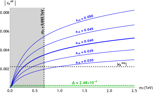
Figure 3: $|\epsilon_{K}^{\text{NP}}|$ as a function of $m_{T}$ in the framework of strict $s_{14}$ dominance ($s_{24}=s_{34}=0$), for various values of $s_{14}$. The vertical line represents the experimental lower bound for the mass of the heavy top, $m_{T}>0.685$ TeV. The black horizontal line corresponds to $|\epsilon^{\text{NP}}_{K}|=|\epsilon^{\text{exp}}_{K}|$, whereas the green one corresponds to $|\epsilon^{\text{NP}}_{K}|=\Delta$. In green we represent the region inside the range of interest for $m_{T}$ where the model might be safe.

However, in the next section, we will show that a small $|\epsilon^{\text{NP}}_{K}|$ obeying $|\epsilon^{\text{NP}}_{K}|\ \lesssim\Delta$, is achievable, if the strict $s_{24}=s_{34}=0$ imposition is dropped and replaced by a more realistic one, where $s_{24},s_{34}\neq 0$, but with $s_{24},s_{34}\ll s_{14}$. This slightly different framework, however, shares the same relevant features as the exact $s_{14}$ dominance case, without changing the pattern of decays and predictions for the heavy top.

3.3 Heavy $T-$ decays

As long as we have that, from all three extra angles, only the angle $s_{14}$ differs from zero, the new heavy $T$ quarks get mixed with the $u$ quark. In the neutral currents, we have $\left|F_{14}^{u}\right|\sim s_{14}$ controlling the decays $T\longrightarrow u\ Z$ and $T\longrightarrow u\ h$. In the charged currents, we have $\left|V_{Td}\right|\sim s_{14}$, $\left|V_{Ts}\right|\sim s_{14}\lambda$ and $\left|V_{Tb}\right|\sim s_{14}\lambda^{3}$, from which one concludes that the dominant decay channel is $T\longrightarrow d\ W$. For the range of masses we consider, one has, to a very good approximation [40]

$$\Gamma\left(T\longrightarrow d\ W\right)\simeq 2\Gamma\left(T\longrightarrow u\ Z\right)\simeq 2\Gamma\left(T\longrightarrow u\ h\right).$$

For experimental purposes, these three decay channels to the light quarks dominate the total decay width. This dominance to light quark channels is a distinctive feature of the $s_{14}$ dominance scenario and is the origin of the fact that we can consider masses as light as $m_{T}$ $=685\ GeV$ [26]. Note that major experimental searches correspond to the channels $\Gamma\left(T\longrightarrow b\ W\right)$, $\Gamma\left(T\longrightarrow t\ Z\right)$, $\Gamma\left(T\longrightarrow t\ h\right)$, here highly suppressed.

4 Solving the $\epsilon_{K}$ problem while maintaining the main features of the $s_{14}-$ dominance case

As stated above, the strict imposition of $s_{24}=s_{34}=0$ above might be considered somewhat unnatural. A possible more realistic scenario would be one, with small, but non-zero $s_{24}$ and $s_{34}$. In this section, we give an analysis of the previous electroweak-precision-measurements (EWPM) related quantities allowing for small values $s_{24},s_{34}\ll s_{14}$

$$s_{34},s_{24}\lesssim\lambda^{5}$$ (30)

while still keeping our solution for CKM unitarity problem with $s_{14}\simeq 0.04$. We show that it is possible to find a suitable solution for the $|\epsilon_{K}|$ problem described in the previous section 3.2, while preserving all the important features of the model, i.e. without significantly affecting predictions for other observables. In addition, we also point out that other important CP-violation quantities, in particular $\epsilon^{\prime}/\epsilon$ and $Br\left(K_{L}\longrightarrow\pi^{0}\nu\overline{\nu}\right)$, require new attention.

4.1 Modifications to the NP contributions in neutral meson mixings

Using the Botella-Chau parametrization, with $c_{13},c_{23},c_{24},$ $c_{34}\simeq 1$ and rephasing the left-handed heavy top quark field as $T_{L}\rightarrow e^{i\delta_{14}}T_{L}$, we parametrize the CKM matrix, in leading order, as presented in Eq. (31) where the $V_{ij}$ represent the $(i,j)$ entries of $\mathcal{V}^{CKM}$ in Eq. (9). Here, we relax one of the upper-bounds in Eq. (30) and assume even that $\left|s_{34}\right|\lesssim\lambda^{5}$ while $\left|s_{24}\right|\lesssim\lambda^{4}$. We have also defined the difference $\delta^{\prime}\equiv\delta_{24}-\delta_{14}$ of the extra phases, which play a role futher on.

$$\begin{array}[]{l}\mathcal{V}^{CKM}=\\ \\ \small{\left(\begin{array}[]{lll}V_{11}&V_{12}&V_{13}\\ V_{21}-c_{12}s_{14}s_{24}e^{-i\delta^{\prime}}&V_{22}-s_{12}s_{14}s_{24}e^{-i\delta^{\prime}}&V_{23}\\ V_{31}-c_{12}s_{14}s_{34}e^{i\delta_{14}}&V_{32}&V_{33}\\ V_{41}+s_{12}s_{24}e^{i\delta^{\prime}}&V_{42}-c_{12}s_{24}e^{i\delta^{\prime}}-c_{12}s_{23}s_{34}e^{-i\delta_{14}}&V_{43}-s_{23}s_{24}e^{i\delta^{\prime}}-s_{34}e^{-i\delta_{14}}\end{array}\right)}\\ \\ +\mathcal{O}(\lambda^{8}),\end{array}$$ (31)

Instead of the expression given in Eq. (23), the overall NP contribution to $|\epsilon_{K}|$ is now approximated by

$$|\epsilon^{\text{NP}}_{K}|\simeq\frac{G_{F}^{2}M_{W}^{2}m_{K}f_{K}^{2}B_{K}\kappa_{\epsilon}}{12\sqrt{2}\pi^{2}\Delta m_{K}}\left|\mathcal{F-F}^{\prime}\right|=q_{K}\left|\mathcal{F-F}^{\prime}\right|,$$ (32)

with $\mathcal{F}^{\prime}$, being an extra contribution to $|\epsilon^{\text{NP}}_{K}|$ coming from the fact that $s_{24},s_{34}\neq 0$.

It is worthwhile to give an approximate expression for this new $|\epsilon_{K}|^{\text{NP}}$, in terms of our BC parametrization in Eqs. (9, 31). In leading order, one finds for Eq. (32),

$$|\epsilon^{\text{NP}}_{K}|=2q_{K}s_{12}s_{14}^{2}\left|\eta_{tT}^{K}S_{tT}s_{13}s_{23}\sin\delta-\eta_{TT}^{K}S_{TT}s_{14}s_{24}\sin\delta^{\prime}\right|.$$ (33)

Note that this leading order contribution to $|\epsilon^{\text{NP}}_{K}|$ is only dependent on the phase combination $\delta^{\prime}=\delta_{24}-\delta_{14}$ and is independent of $s_{34}$, because we chose $s_{34}\leq\lambda^{5}$. In fact, this also true for the next-leading order terms.

From Eq. (33), it is already clear that $|\epsilon^{\text{NP}}_{K}|$ may become small in certain regions of parameter-space, if the two terms in the expression can cancel each other. Moreover, if we restrict ourselves to a region of the mass $m_{T}$ (of the extra heavy quark) between $5m_{t}\leq m_{T}\leq 12m_{t}$, then with Eqs. (17, 18), we find that $\eta_{tT}^{K}\ S_{tT}$ and $\eta_{TT}^{K}\ S_{TT}$ in Eq. (33) behave, in a good approximation, as linear functions of $k=\frac{m_{T}}{m_{t}}$

$$\begin{array}[]{c}\eta_{tT}^{K}S_{tT}\approx 2.492+0.1492\ k,\\ \\ \eta_{TT}^{K}S_{TT}\approx-36.613+10.232\ k.\end{array}$$ (34)

With this simplification and with the PDG values for $s_{13}$, $s_{23}$ as well as our proposed value for $s_{14}\approx 0.04$, one finds that there exists a fairly large parameter region (depending on $\theta_{24}$) which is allowed for $\delta^{\prime}$ and where $\delta^{\prime}\in\left[1.0,2.0\right]$. Thus, we find that this new phase $\delta^{\prime}$ assumes values, in this context, which are very similar to the usual CP-violating phase $\delta$.

In figure 4, we plot Eq. (32) for various values of $s_{24}$, using Eq. (29) with $s_{14}=0.04$ and a central value for $\sin\delta^{\prime}=1$. From the plot we conclude that small values of $|\epsilon^{\text{NP}}_{K}|$ can be achieved, e.g. for $m_{T}=0.685$ TeV by having $s_{24}\lesssim 1.2\times 10^{-3}$, or e.g. for $m_{T}=1.0$ TeV by having $s_{24}\lesssim 6\times 10^{-4}$. Thus, we find a region where the problem discussed in section 3.2 can be fixed. In addition, one can see that having $s_{24}<2\times 10^{-4}$ is undesirable as it would require very large heavy top masses ($m_{T}\gtrsim 2$ TeV) to achieve $|\epsilon_{K}|^{\text{NP}}\lesssim\Delta.$

The NP contributions to $\Delta m_{B_{i}}$ will also be modified, with all changes coming essentially from $\lambda_{T}^{B_{i}}$. From Eq. (31) one finds for $s_{34}\sim\lambda^{5}$, in leading order

$$\begin{split}\lambda_{T}^{B_{d}}\simeq V_{41}V_{43}^{*}\left(1-\frac{s_{34}}{V_{43}^{*}}e^{i\delta_{14}}\right),\\ \\ \lambda_{T}^{B_{s}}\simeq V_{42}V_{43}^{*}\left(1-\frac{s_{34}}{V_{43}^{*}}e^{i\delta_{14}}\right),\end{split}$$ (35)

so that now, we have an extra term for each quantity which competes with the absolute dominance result. For $s_{34}\sim|V_{43}|\sim\lambda^{5}$ the new term will be of the order of the old one, which should not be problematic given how insignificant the NP contributions to $\Delta m_{B_{i}}$ are in the absolute dominance framework.

Still, if one requires that in this alternative framework the predictions for $\Delta m^{\text{NP}}_{B_{i}}$ do not differ significantly from the ones of absolute dominance, then Eq. (35) seems to favor $s_{34}\ll|V_{43}|\sim\lambda^{5}$ and we are able to recover the results of absolute dominance. This fact, when coupled with the independence of Eq. (33) on $s_{34}$ suggests that the $s_{14}$ dominance framework might be viable even with $s_{34}\ll s_{24}$. On the other hand, the observable $\Delta m_{K}$ will not be meaningfully altered when switching to Eq. (30) as the new terms in Eq. (31) which contribute to $\lambda_{T}^{K}$ are dominated by $|V_{41}|\sim\lambda^{2}$ and $|V_{42}|\sim\lambda^{3}$.

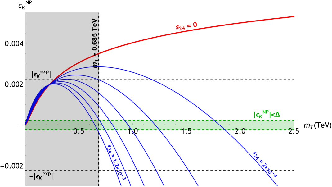
Figure 4: Analogous plot to that of figure 3 but for realistic dominance with $\theta_{14}=0.04$ and $\delta^{\prime}=\pi/2$. Various values of $s_{24}$ are spanned in steps of $2\times 10^{-4}$ for $s_{24}\in[0,1.2\times 10^{-3}]$. The curve for $s_{24}=0$ (in red) is the thicker one in figure 3. The region $|\epsilon_{K}|^{\text{NP}}<\Delta$ is highlighted in green for $m_{T}>0.685$ TeV.

4.2 Emergence of more New Physics

Having non-zero $s_{24}$ and $s_{34}$ implies non-zero $\mathcal{V}_{42}$ and $\mathcal{V}_{43}$ which in turn will induce NP contributions to $D^{0}-\overline{D}^{0}$ mixing and allow rare decays of the top quark into the lighter generations, which was not true before. We now will briefly study these processes, as well as others, like $K_{L}\rightarrow\pi^{0}\overline{\nu}\nu$ and the CP violation observable $\epsilon^{\prime}/\epsilon$.

$D^{0}-\overline{D}^{0}$ mixing

The NP tree-level contribution to the $D^{0}-\overline{D}^{0}$ mixing is described by the effective Lagrangian [42]

$$\mathcal{L}_{\text{eff}}^{\text{NP}}=-\frac{G_{F}}{\sqrt{2}}\ (\mathcal{V}_{41}^{u*}\mathcal{V}_{42}^{u})^{2}\ (\overline{u}_{L}\gamma^{\mu}c_{L})(\overline{u}_{L}\gamma_{\mu}c_{L}),$$ (36)

This results in a contribution to the $D^{0}$ mixing parameter $x_{D}\equiv\Delta m_{D}/\Gamma_{D}$ given by [43]

$$x_{D}^{\text{NP}}\simeq\frac{\sqrt{2}m_{D}}{3\Gamma_{D}}\ G_{F}\ f_{D}^{2}\ B_{D}\ r(m_{c},M_{Z})\ |\mathcal{V}_{41}^{u*}\mathcal{V}_{42}^{u}|^{2}.$$ (37)

where $r(m_{c},M_{Z})\simeq 0.778$ is a factor that accounts for RG effects. The remaining constants are $m_{D}=1864.83\pm 0.05$ MeV, $\Gamma_{D}=1/\tau_{D}$ with $\tau_{D}=(410.1\pm 1.5)\times 10^{-15}$ s [25], $B_{D}=1.18_{-0.05}^{+0.07}$ [44] and $f_{D}=212.0\pm 0.7$ MeV [36]. Requiring $s_{24}\lesssim\lambda^{5}$ yields an upper bound for the NP contribution of $x_{D}^{\text{NP}}<0.015\%$, which is negligible when compared to the experimental value, $x_{D}^{\text{exp}}=0.39_{-0.12}^{+0.11}\%$ [45].

Figure 5: NP contribution to $D^{0}-\overline{D}^{0}$ mixing via $Z$-mediated FCNC.

Rare $t\rightarrow qZ$ decays

With $s_{34}\neq 0$, the mixing of the VLQ with the lighter generations will result in rates for the processes $t\rightarrow q_{i}Z$, ($q_{i}=u,c$) which may differ significantly from the ones predicted by the SM. In fact, the leading-order NP contribution occurs at tree-level and is given by [46]

$$\Gamma(t\rightarrow q_{i}Z)_{\text{NP}}\simeq\frac{\alpha}{32s_{W}^{2}c_{W}^{2}}|\mathcal{V}_{4i}^{u*}\mathcal{V}_{43}^{u}|^{2}\frac{m_{t}^{3}}{M_{Z}^{2}}\left(1-\frac{M_{Z}^{2}}{m_{t}^{2}}\right)^{2}\left(1+2\frac{M_{Z}^{2}}{m_{t}^{2}}\right).$$ (38)

Approximating the total decay width of the top-quark by $\Gamma_{t}\simeq\Gamma(t\rightarrow bW^{+})$, the branching ratio is

$$\text{Br}(t\rightarrow q_{i}Z)_{\text{NP}}\simeq\frac{|\mathcal{V}_{4i}^{u\ast}\mathcal{V}_{43}^{u}|^{2}}{2|V_{33}|^{2}}\left(1-\frac{M_{Z}^{2}}{m_{t}^{2}}\right)^{2}\left(1+2\frac{M_{Z}^{2}}{m_{t}^{2}}\right)\left(1-3\frac{M_{Z}^{4}}{m_{t}^{4}}+2\frac{M_{Z}^{6}}{m_{t}^{6}}\right)^{-1}.$$ (39)

However, for $s_{24},s_{34}\lesssim\lambda^{5}$, it will never come close to exceed the experimental upper bounds: $\text{Br}(t\rightarrow uZ)_{\text{exp}}<1.7\times 10^{-4}$, $\text{Br}(t\rightarrow cZ)_{\text{exp}}<2.4\times 10^{-4}$ (95% CL) [47]. For $s_{34}\sim 10^{-7}$, one might even conceivably achieve NP contributions lower than the SM predictions $\text{Br}(t\rightarrow uZ)_{\text{SM}}\sim 10^{-16}$, $\text{Br}(t\rightarrow cZ)_{\text{SM}}\sim 10^{-14}$ [46].

The decay $K_{L}\rightarrow\pi^{0}\overline{\nu}\nu$

For this process, it is relevant to study the quantity $L$ proportional to the decay amplitude, which in the SM and using the standard PDG parametrization, can be written as [28]

$$L_{SM}=|\text{Im}\left[\lambda_{c}^{K}\ X(x_{c})+\lambda_{t}^{K}\ X(x_{t})\right]|^{2},$$ (40)

where we have introduced an extra Inami-Lim function $X(x_{i})$, presented in Eq. (71) of Appendix B.

When the heavy-top is introduced two new terms should be added to Eq. (40), leading to

$$L=|\text{Im}\left[\lambda_{c}^{K}\ X(x_{c})+\lambda_{t}^{K}\ X(x_{t})+\lambda_{T}^{K}\ X(x_{T})+A_{ds}\right]|^{2}.$$ (41)

The first term is a simple generalisation of the terms in Eq. (40) which is to be expected from the introduction of a new quark, whereas the last one accounts for the decoupling behaviour that arises from the fact that this new quark is an isosinglet and is responsible for generating FCNC’s at tree level in the electroweak sector. Note that the gauge-invariant function in Eq. (71) is obtained by considering all diagrams that contribute to processes such as $K_{L}\rightarrow\pi^{0}\overline{\nu}\nu$, with some of these diagrams being $Z$-exchange penguin diagrams where we can have up-type quarks running inside a loop coupled to a $Z$-boson, $i.e$ where the new FCNC’s effects in the up quark sector have to be taken into account. The role of $A_{ds}$ is, therefore, to account for these effects.

With regard to $A_{ds}$, we have [52]–[56]

$$A_{ds}=\sum_{i,j=c,t,T}V_{is}^{*}\left(F^{u}-I\right)_{ij}V_{jd}N(x_{i},x_{j}),$$ (42)

with

$$\begin{split}N(x_{i},x_{j})=\frac{x_{i}x_{j}}{8}\left(\frac{\log x_{i}-\log x_{j}}{x_{i}-x_{j}}\right),\\ \\ N(x_{i},x_{i})\equiv\lim_{x_{j}\rightarrow x_{i}}N(x_{i},x_{j})=\frac{x_{i}}{8}.\end{split}$$ (43)

For $s_{24}\neq 0$ and in the limit $s_{34}=0$, the FCNC-matrix $F^{u}$ in Eq. (10) gets modified into

$$\small F^{u}=\left(\begin{array}[]{cccc}c_{14}^{2}&-c_{14}s_{14}s_{24}e^{i\delta^{\prime}}&0&-c_{14}c_{24}s_{14}e^{-i\delta_{14}}\\ -c_{14}s_{14}s_{24}e^{-i\delta^{\prime}}&1-c_{14}^{2}s_{24}^{2}&0&-c_{14}^{2}c_{24}s_{24}e^{-i\delta_{24}}\\ 0&0&1&0\\ -c_{14}c_{24}s_{14}e^{i\delta_{14}}&-c_{14}^{2}c_{24}s_{24}e^{i\delta_{24}}&0&1-c_{14}^{2}c_{24}^{2}\end{array}\right),$$ (44)

So that to a very good approximation one can write

$$A_{ds}\simeq-\frac{x_{T}}{8}c^{2}_{14}c^{2}_{24}\lambda^{K}_{T}.$$ (45)

Thus, we obtain

$$L\simeq|\text{Im}\left[\lambda_{c}^{K}X(x_{c})+\lambda_{t}^{K}X(x_{t})+\lambda_{T}^{K}\tilde{X}(x_{T})\right]|^{2},$$ (46)

where, with $c_{14},c_{24}\simeq 1$, we have defined

$$\tilde{X}(x_{T})\equiv X(x_{T})-\frac{x_{T}}{8}=\frac{x_{T}}{8(x_{T}-1)}\left(3+\frac{3x_{T}-6}{x_{T}-1}\log x_{T}\right),$$ (47)

which shows the logarithmic behaviour of the NP piece. From Eq. (9) it is clear that in the limit $s_{24}=0$ there is essentially no NP piece, given that $\text{Im}\lambda_{T}^{K}=0$. However, if one takes $s_{24}\neq 0$ in order to fix the $\epsilon_{K}$ problem, this is no longer true as $\text{Im}\lambda_{T}^{K}\simeq-c_{12}^{2}s_{14}s_{24}\sin\delta^{\prime}$. In the considered range of parameters, we can get, in general, an important reduction of the branching ratio of the CP violation decay $K_{L}\rightarrow\pi^{0}\overline{\nu}\nu$

$$0.2\lesssim\frac{L}{L_{\text{SM}}}\simeq\frac{\text{Br}\left(K_{L}\rightarrow\pi^{0}\overline{\nu}\nu\right)}{\text{Br}\left(K_{L}\rightarrow\pi^{0}\overline{\nu}\nu\right)_{\text{SM}}}\lesssim 0.8.$$ (48)

The decay $K^{+}\rightarrow\pi^{+}\overline{\nu}\nu$

Similarly, this process is studied analysing the ratio

$$\frac{L^{+}}{L^{+}_{\text{SM}}}\equiv\frac{\text{Br}(K^{+}\rightarrow\pi^{+}\overline{\nu}\nu)}{\text{Br}(K^{+}\rightarrow\pi^{+}\overline{\nu}\nu)_{\text{SM}}}=\left|\frac{\lambda_{c}^{K}X^{\text{NNL}}(x_{c})+\lambda_{t}^{K}X(x_{t})+\lambda_{T}^{K}X(x_{T})+A_{ds}}{\lambda_{c}^{K}X^{\text{NNL}}(x_{c})+\lambda_{t}^{K}X(x_{t})}\right|^{2},$$ (49)

where, here, the charm contribution cannot be overlooked, because, even though $X^{\text{NNL}}(x_{c})\ll X(x_{t})$, one has that $\lambda_{c}^{K}\gg\lambda_{t}^{K}$. Also, instead of the previous charm contribution $X(x_{c})$, we now use the NNLO [57] charm contribution $X^{\text{NNL}}(x_{c})\simeq 1.04\times 10^{-3}$ (see Appendix B).

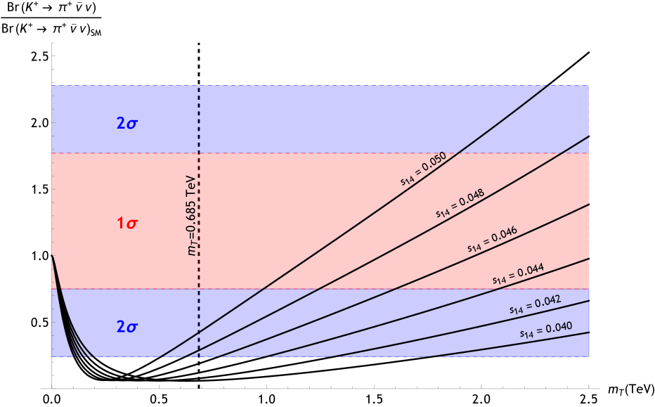
Figure 6: Plot of Eq. (49) as a function of $m_{T}$ for various values of $s_{14}\geq 0.04$ with $s_{24}=s_{34}=5\times 10^{-4}$, $\delta^{\prime}=1.2$ and using Eq. (29). The coloured regions refer to the $1\sigma$ and $2\sigma$ ranges.

Current measurements of this decay yield $\text{Br}(K^{+}\rightarrow\pi^{+}\overline{\nu}\nu)_{\text{exp}}=\left(10.6_{-3.4}^{+4.0}\pm 0.9\right)\times 10^{-11}$, whereas the SM prediction is $\text{Br}(K^{+}\rightarrow\pi^{+}\overline{\nu}\nu)_{\text{SM}}=\left(8.4\pm 1.0\right)\times 10^{-11}$ [58]. One may establish the following rough $1\sigma$ range for the ratio in Eq. (49)

$$\begin{split}\left(\frac{L^{+}}{L^{+}_{\text{SM}}}\right)=1.26\pm 0.51,\end{split}$$ (50)

which has a significant uncertainty due to considerable experimental errors for the branching ratio. However, it may still set constraints on VLQ-extensions of the SM, as is the case of the $s_{14}$ dominance limit. For our model, it seems that larger values of $s_{14}$ are favoured and smaller values for $m_{T}$ disfavoured, as can be seen from the plots in figure 6. We consider a $95\%$ CL region where $s_{14}\in[0.03,0.05]$.

Evaluation of $\epsilon^{\prime}/\epsilon$

The parameter $\epsilon^{\prime}/\epsilon$ measures direct CP violation in $K_{L}\rightarrow\pi\pi$ decays. The SM contribution can be described by the simplified expression [49]

$$\left(\frac{\epsilon^{\prime}}{\epsilon}\right)_{\text{SM}}\simeq F(x_{t})\text{Im}(\lambda_{t}^{K})$$

with

$$F(x_{i})=P_{0}+P_{X}X(x_{i})+P_{Y}Y(x_{i})+P_{Z}Z(x_{i})+P_{E}E(x_{i}),$$ (51)

where the Inami-Lim functions and the associated constants are detailed in Appendix B.

In a similar fashion as was done in the previous subsection, we will now estimate the NP contribution, with

$$\left(\frac{\epsilon^{\prime}}{\epsilon}\right)_{\text{NP}}\simeq F(x_{T})\ \text{Im}(\lambda_{T}^{K})+(P_{X}+P_{Y}+P_{Z})\ \text{Im}(A_{ds}),$$ (52)

where the second term accounts for the decoupling associated with the EW penguin diagrams from which the Inami-Lim functions $X(x_{i}),Y(x_{i})$ and $Z(x_{i})$ are obtained [48]. In this expression, we assume that the constants present in $F(x_{t})$ and $F(x_{T})$ have the same values.

Using Eq. (45) and $c_{14},c_{24}\simeq 1$, one can write

$$\left(\frac{\epsilon^{\prime}}{\epsilon}\right)^{\text{NP}}\simeq\tilde{F}(x_{i})\text{Im}(\lambda_{T}^{K})\simeq-\tilde{F}(x_{i})c_{12}^{2}s_{14}s_{24}\sin\delta^{\prime},$$ (53)

where $\tilde{F}(x_{T})\equiv F(x_{T})-\frac{x_{T}}{8}\left(P_{X}+P_{Y}+P_{Z}\right)$ evolves logarithmically with $x_{T}$. Once more it obvious that in the strict $s_{14}$ dominance limit there is no NP contribution.

For $s_{24}\neq 0$, one may use [51]

$$-4\times 10^{-4}\lesssim\left(\frac{\epsilon^{\prime}}{\epsilon}\right)^{\text{NP}}\lesssim 10\times 10^{-4},$$ (54)

as a rough $1\sigma$ range for $\left(\epsilon^{\prime}/\epsilon\right)_{\text{NP}}$. Taking into account that $\sin\delta^{\prime}>0$ is needed to solve the $\epsilon_{K}$ problem, one can easily fulfil the condition in Eq. (54) for $s_{24}\lesssim 7.5\times 10^{-4}$ in the mass range $m_{T}\in[0.685,15]$ TeV, with this allowed range becoming larger as $s_{24}$ decreases. Therefore, the realistic $s_{14}$ dominance limit should be safe with regard to $\left(\epsilon^{\prime}/\epsilon\right)$.

Global Analysis

Finally, we find it instructive to present a global analysis of the most relevant phenomenological restrictions of parameter space which apply to our $s_{14}-$dominance model, in particular, the allowed parameter range for $s_{14},s_{24},\delta^{\prime}$ and $m_{T}$.

In figure 7, we present several slice-projections of the allowed parameter region combining the most important parameters. The values for $s_{14}$ are in accordance with the solution proposed for the CKM unitarity problem, and $s_{24},s_{34}$ are within our assumptions for $s_{14}$-dominance. More concretely the parameter range for these parameters are

$$\begin{array}[]{c}m_{T}\in[0.685,2.5]\ \text{TeV},\\ \\ s_{14}\in[0.03,0.05],\\ \\ s_{24},s_{34}\in[0,0.001],\\ \\ \delta_{14},\delta_{24}\in[0,2\pi],\end{array}$$ (55)

and we impose the constraint

$$\Delta m_{K}^{\text{NP}}<\Delta m_{K}^{\text{exp}}$$ (56)

on the model. We also look for regions that may be accessible to upcoming generations of accelerators and therefore restrict ourselves to the study of models with masses lower than $m_{T}=2.5$ TeV. This is in agreement with the upper-bound presented in [12] for models with an heavy-top where $|\mathcal{V}_{41}|\simeq 0.04$.

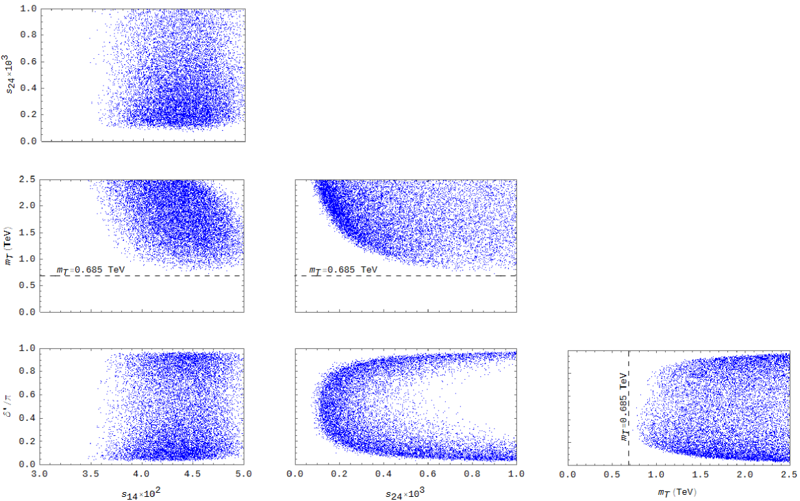
Figure 7: Results for the allowed parameter regions of our model verifying the conditions in Eqs. (55, 56) and $\sqrt{\chi^{2}}<3$.

The points displayed in figure 7 correspond to points that not only verify Eq. (56) but also deviate less than $3\sigma$ from current experimental data, with $n\sigma$ defined as $n\sigma=\sqrt{\chi^{2}}$ and

$$\begin{split}\chi^{2}=&\sum_{i,j}\left(\frac{|V_{ij}|-|V_{ij}|_{c}}{\sigma_{ij}}\right)^{2}+\left(\frac{\gamma-\gamma_{c}}{\sigma_{\gamma}}\right)^{2}\\ &+\left(\frac{|\varepsilon^{\text{NP}}_{K}|-|\varepsilon^{\text{NP}}_{K}|_{c}}{\sigma_{\varepsilon}}\right)^{2}+\left(\frac{\left(L^{+}/L^{+}_{\text{SM}}\right)-\left(L^{+}/L^{+}_{\text{SM}}\right)_{c}}{\sigma_{L}}\right)^{2}\\ &+\left(\frac{\left(\epsilon^{\prime}/\epsilon\right)^{\text{NP}}-\left(\epsilon^{\prime}/\epsilon\right)^{\text{NP}}_{c}}{\sigma_{\epsilon^{\prime}/\epsilon}}\right)^{2}\end{split}$$ (57)

where for $|V_{ij}|$ we take the most relevant moduli of the SM mixing matrix entries, given by the PDG [25], as well as the value of the rephasing invariant phase $\gamma\equiv\text{arg}(-V_{ud}V_{cb}$ $V^{\ast}_{ub}V^{\ast}_{cd})$. The measurement of this quantity is associated with SM tree-level dominated $B$-meson physics and is, therefore, expected to remain unaffected in a model like ours, as referred also in [25]. Taking into account the current value of $\gamma=\left(72.1^{+4.1}_{-4.5}\right)^{\circ}$ we consider a central value for $\gamma_{c}=72.1^{\circ}$ and $\sigma_{\gamma}=4.5^{\circ}$ for the standard deviation.

We use a similar methodology to the one presented in [11], but now adding more terms to $\chi^{2}$. E.g. we include the NP contribution to $\varepsilon_{K}$ and the new insights discussed in Eq. (3.2), with regions of parameter space where $|\epsilon^{\text{NP}}_{K}|\leq|\epsilon^{\text{exp}}_{K}|-|\epsilon^{\text{SM}}_{K}|\simeq 6.8\times 10^{-5}$. We also take into account the NP contributions associated to the decay $K^{+}\rightarrow\pi^{+}\overline{\nu}\nu$ and the parameter $\varepsilon^{\prime}/\varepsilon$. The constraints set by these observables lead to the lower-bound for a heavy-top mass of around $m_{T}\approx 800$ GeV apparent from figure 7. Additionally, the kaon decay in particular restricts the allowed range of $s_{14}$ to roughly $s_{14}\in[0.035,0.050]$ as figure 6 previously suggested.

Note that we do not include constraints associated with other observables, such as $\Delta m_{B_{d,s}}$ and $x_{D}$, because, as it was shown, their NP contributions are extremely suppressed in the limit of $s_{14}$ dominance. Furthermore, plots involving $s_{34}$ are omitted as, within the range in Eq. (55), there is no noticeable influence of importance on the outcome of the allowed parameter region.

In the Example II of Appendix A we present a numerical case with a mass $m_{T}=1477$ GeV for the extra heavy up-quark and

$$\begin{array}[]{lllll}\theta_{12}=0.22579,&&\theta_{13}=0.0038275,&&\theta_{23}=0.039524,\\ \\ \theta_{14}=0.045334,&&\theta_{24}=7.412\times 10^{-4},&&\theta_{34}=2.346\times 10^{-4},\\ \\ \delta=0.382\pi,&&\delta_{14}=1.872\pi,&&\delta_{24}=1.979\pi.\\ \end{array}$$ (58)

leading to $\sqrt{\chi^{2}}\simeq 2.25$.

5 Conclusions

We have shown that there is a minimal extension of the SM involving the introduction of an up-type vector-like quark $T$, which provides a simple solution to the CKM unitarity problem. The heavy quark $T$ decays dominantly to light quarks, in contrast with the usual assumption that $T$ decays predominantly to the $b$ quark. Therefore, these unusual $T$ decay patterns should be taken into account in the experimental search for vector-like quarks. We have adopted the Botella-Chau parametrization of a $4\times 4$ unitary matrix which, in contrast to the PDG parametrization, has three more angles $s_{14}$, $s_{24}$ and $s_{34}$ and two extra phases.

We have shown that New Physics contributions e.g. to $K^{0}-\overline{K}^{0}$ and $B_{d,s}^{0}-\overline{B}_{d,s}^{0}$ mixing or in the decays $K_{L}\rightarrow\pi^{0}\overline{\nu}\nu$, $K^{+}\rightarrow\pi^{+}\overline{\nu}\nu$ and new contributions to $\epsilon^{\prime}/\epsilon$ can be well within the limits of EWPM’s.

We have also used a recently introduced upper-bound on $|\epsilon^{\text{NP}}_{K}|$, which severely restricts various models, to test our own model with exact $s_{14}$ dominance.

We have pointed out that, in the limit of exact $s_{14}$ dominance, the new contribution to $\epsilon_{K}$ is too large. When this limit is relaxed, allowing for a non-vanishing angle $s_{24}$, we then show that the leading order terms of $|\epsilon^{\text{NP}}_{K}|$ can be expressed as the sum of terms proportional to the usual CP-violating PDG phase $\delta$ and terms that are proportional to a new phase $\delta^{\prime}=\delta_{24}-\delta_{14}$, i.e. to the difference of the other two phases of the BC parametrization. One can then check that there exists a reasonable parameter region, where these two terms may cancel each other, and that allows for the mass of the $T$ quark to vary between around $800$ GeV and $2.5$ TeV. Thus, we find that the New Physics contribution to $\epsilon_{K}$ can be agreement with the set upper-bound, and therefore with experiment, without changing the main predictions of the model, in particular the predicted pattern of $T$ decays.

Appendix A Numerical Examples

To stress and exemplify the claims made here, we give, in this Appendix, two exact numerical examples.

Example I: Absolute dominance

As an example of exact $s_{14}$ dominance, consider the following up-sector mass matrix

$$\small\mathcal{M}_{u}=\left(\begin{array}[]{cccc}0&0&0&65.2612\\ 0&0&7.09671&14.848e^{1.94715i}\\ 0&19.3662&172.739&3.82017e^{-1.5659i}\\ 0.0397187&1.63395&32.6789e^{-1.51428i}&1475.32\\ \end{array}\right),$$ (59)

given in GeV at the $M_{Z}$ scale. The up-type quark masses are then, at this scale,

$$\begin{array}[]{cc}m_{u}=0.0018\text{ GeV},&m_{c}=0.77\text{ GeV},\\ \\ m_{t}=174\text{ GeV},&m_{T}=1477\text{ GeV}.\end{array}$$ (60)

In the basis where the down sector mass matrix is diagonal, the matrix $\mathcal{V}^{\dagger}$ which diagonalizes $\mathcal{M}_{u}$ on the left will have absolute value

$$\small|\mathcal{V}^{\dagger}|\simeq\left(\begin{array}[]{cccc}0.973609&0.223644&0.00382359&0.0453188\\ 0.223754&0.973844&0.0395133&0.\\ 0.008257&0.03883&0.999212&0.\\ 0.0441681&0.0101457&0.000173458&0.998973\\ \end{array}\right)$$ (61)

Recall that $\mathcal{V}^{CKM}$ is given by a $4\times 3$ matrix of the first three columns of this matrix.

We obtain also for the rephasing invariant phases

$$\begin{array}[]{c}\sin(2\beta)\equiv\sin\left[2\ \text{arg}\left(-V_{cd}V_{tb}V^{\ast}_{cb}V^{\ast}_{td}\right)\right]\simeq 0.764,\\ \\ \gamma\equiv\text{arg}\left(-V_{ud}V_{cb}V^{\ast}_{ub}V^{\ast}_{cd}\right)\simeq 68.7^{\circ},\\ \\ \beta_{s}\equiv\text{arg}\left(-V_{cb}V_{ts}V^{\ast}_{cs}V^{\ast}_{tb}\right)\simeq 0.0206,\\ \\ \beta_{K}\equiv\text{arg}\left(-V_{us}V_{cd}V^{\ast}_{ud}V^{\ast}_{cs}\right)\simeq 6.464\times 10^{-4},\\ \end{array}$$ (62)

and the CP-violation invariant, defined as

$$J\equiv\text{Im}\left(V_{us}V_{cb}V_{ub}^{*}V_{cs}^{*}\right),$$ (63)

has absolute value $|J|=3.070\times 10^{-5}$.

For the EWPMs related quantities discussed above, we obtain the following NP contributions

$$\begin{array}[]{c}\Delta m_{B_{d}}^{\text{NP}}\simeq 1.726\times 10^{-12}\hskip 2.84526pt\text{MeV},\\ \\ \Delta m_{B_{s}}^{\text{NP}}\simeq 2.892\times 10^{-12}\hskip 2.84526pt\text{MeV},\\ \\ \Delta m_{K}^{\text{NP}}\simeq 1.192\times 10^{-13}\hskip 2.84526pt\text{MeV},\\ \\ |\epsilon^{\text{NP}}_{K}|\ \simeq 5.889\times 10^{-3},\end{array}$$ (64)

which, as stated, clearly emphasises the problem with the limit $s_{24}=s_{34}=0$ and the value for the parameter $|\epsilon_{K}|$.

Example II: Realistic dominance with very small $s_{24},s_{34}$

To exemplify a more realistic case near to our exact $s_{14}$ dominance, but with very small $s_{24},s_{34}$, we now consider a slightly different up-mass matrix (in $GeV$ at the $M_{Z}$ scale)

$$\small\mathcal{M}_{u}=\left(\begin{array}[]{cccc}0&0&0&65.033\\ 0&0&7.12124&15.8436e^{1.92462i}\\ 0&19.3672&172.73&4.21828e^{-1.56762i}\\ 0.0397187&1.63403&32.7938e^{-1.51551i}&1475.32\\ \end{array}\right),$$ (65)

which leads to the same mass spectrum as the one in Eq. (60) and to

$$\small|\mathcal{V}^{\dagger}|\simeq\left(\begin{array}[]{cccc}0.973609&0.223644&0.00382359&0.0453188\\ 0.223785&0.973837&0.0395133&0.000740405\\ 0.00824668&0.0388324&0.999212&0.000234355\\ 0.0440136&0.010821&0.000312045&0.998972\\ \end{array}\right).$$ (66)

The rephasing invariant phases are very similar

$$\begin{array}[]{cc}\sin(2\beta)\simeq 0.764,&\gamma\simeq 68.7^{\circ},\\ \\ \beta_{s}\simeq 0.0206,&\beta_{K}\simeq 5.950\times 10^{-4},\end{array}$$ (67)

as is the CP-violating invariant $|J|=3.070\times 10^{-5}$.

The observables associated with the EWPMs have the following NP contributions

$$\begin{array}[]{c}\Delta m_{B_{d}}^{\text{NP}}\simeq 3.119\times 10^{-12}\hskip 2.84526pt\text{MeV},\\ \\ \Delta m_{B_{s}}^{\text{NP}}\simeq 5.547\times 10^{-12}\hskip 2.84526pt\text{MeV},\\ \\ \Delta m_{K}^{\text{NP}}\simeq 1.356\times 10^{-12}\hskip 2.84526pt\text{MeV},\\ \\ |\epsilon^{\text{NP}}_{K}|\ \simeq 6.592\times 10^{-5},\end{array}$$ (68)

As it is clear, the problem with $\epsilon_{K}$ is now successfully solved. Comparing Eq. (64) and Eq. (68) one also sees that although noticeable changes to $\Delta m_{B_{d}}^{\text{NP}}$ and $\Delta m_{Bs}^{\text{NP}}$ took place, these are still small and in no way compromise the safety of the model.

Appendix B Inami-Lim functions

The Inami-Lim functions used throughout this paper are given by [29, 48]

$$S_{ij}\equiv S(x_{i},x_{j})=x_{i}x_{j}\left[\frac{\log x_{i}\left(1-2x_{i}+\frac{x_{i}^{2}}{4}\right)}{(x_{i}-x_{j})(1-x_{i})^{2}}+(x_{i}\leftrightarrow x_{j})\right]-\frac{3x_{i}x_{j}}{4(1-x_{i})(1-x_{j})},$$ (69)

$$S_{i}\equiv S(x_{i})\equiv\lim_{x_{j}\rightarrow x_{i}}S(x_{i},x_{j})=\frac{x_{i}}{(1-x_{i})^{2}}\left(1-\frac{11}{4}x_{i}+\frac{x_{i}^{2}}{4}\right)-\frac{3}{2}\frac{x_{i}^{3}\log x_{i}}{(1-x_{i})^{3}},$$ (70)

$$X(x_{i})=\frac{x_{i}}{8(x_{i}-1)}\left(x_{i}+2+\frac{3x_{i}-6}{x_{i}-1}\log x_{i}\right),$$ (71)

$$Y(x_{i})=\frac{x_{i}}{8(x_{i}-1)}\left(x_{i}-4+\frac{3x}{x_{i}-1}\log x_{i}\right),$$ (72)

$$Z(x_{i})=-\frac{\log x_{i}}{9}+\frac{18x^{4}_{i}-163x^{3}_{i}+259x^{2}_{i}-108x_{i}}{144(x_{i}-1)^{3}}+\frac{32x^{4}_{i}-38x^{3}_{i}-15x^{2}_{i}+18x_{i}}{72(x_{i}-1)^{4}}\log x_{i},$$ (73)

$$E(x_{i})=-\frac{2\log x_{i}}{3}+\frac{x_{i}(18-11x_{i}-x_{i}^{2})}{12(1-x_{i})^{3}}+\frac{x_{i}^{2}(15-16x_{i}+4x_{i}^{2})}{6(1-x_{i})^{4}}\log x_{i}.$$ (74)

All these functions are gauge invariant, however, $X(x_{i}),$ $Y(x_{i})$ and $Z(x_{i})$ correspond to linear combinations of gauge-dependent functions. $X(x_{i})$ and $Y(x_{i})$ are obtained by combining box functions with $Z$ penguin functions, whereas $Z(x_{i})$ is obtained by combining photon and $Z$ penguin functions. $S(x_{i},x_{j})$ is a box diagram function that is relevant in meson mixings and $E(x_{i})$ is associated with gluon penguins.

The function $F(x_{i})$ in Eq. (51), relevant to the study of $\epsilon^{\prime}/\epsilon$, is a linear combination of $X(x_{i}),Y(x_{i}),Z(x_{i})$ and $E(x_{i})$. We use the following values for the constants entering this expression [50]

$$\begin{array}[]{c}P_{0}\simeq-3.392+15.3037\ B_{6}^{(1/2)}+1.7111\ B_{8}^{(3/2)},\\ \\ P_{X}\simeq 0.655+0.02902\ B_{6}^{(1/2)},\\ \\ P_{Y}\simeq 0.451+0.1141\ B_{6}^{(1/2)},\\ \\ P_{Z}\simeq 0.406-0.0220\ B_{6}^{(1/2)}-13.4434\ B_{8}^{(3/2)},\\ \\ P_{E}\simeq 0.229-1.7612\ B_{6}^{(1/2)}+0.6525\ B_{8}^{(3/2)},\end{array}$$ (75)

as well as the central values of $B_{6}^{(1/2)}=1.11\pm 0.20$ and $B_{8}^{(3/2)}=0.70\pm 0.04$ [51].

The correction $X^{\text{NNL}}(x_{c})$ used in Eq. (49) is important because, as mentioned above, the Inami-Lim function $X(x_{i})$ is obtained from combining the contributions of penguin and box diagrams to neutrino decays of mesons. For the kaon case, the relevant box diagrams are the ones presented in figure (8).

Figure 8: Box diagram contributing to $K_{L}\rightarrow\pi^{0}\overline{\nu}\nu$ and $K^{+}\rightarrow\pi^{+}\overline{\nu}\nu$, from which $X(x_{i})$ in Eq. (71) is obtained, with $u_{i,j}=u,c,t,T$ and $\ell=e,\mu,\tau$.

The expression for $X(x_{i})$ in Eq. (71) is obtained by taking the limit of vanishing masses for the leptons involved in the loop so that this function involves solely the mass of the up-type quark running inside the loop. This is a good approximation for the top and heavy top contributions given that $m_{t},m_{T}\gg m_{\tau}$, however for the charm quark one has $m_{c}<m_{\tau}$ and Eq. (71) is no longer valid. Hence, it should be replaced by

$$X^{\text{NNL}}(x_{c})=X_{\text{SD}}^{\text{NNL}}(x_{c})+\delta X(x_{c}),$$ (76)

where $\delta X(x_{c})$ is the long-distance contribution. The short-distance piece is, at NNLO, given by

$$X_{\text{SD}}^{\text{NNL}}(x_{c})=\frac{2}{3}X_{e}^{\text{NNL}}(x_{c})+\frac{1}{3}X_{\tau}^{\text{NNL}}(x_{c}),$$ (77)

so that the contributions involving the lepton $\tau$ and the remaining lighter leptons are considered separately. Following [57] one can approximate this quantity with $X^{\text{NNL}}(x_{c})\simeq 1.04\times 10^{-3}$.