Quark mass RG-running for $N_{f}$ =3 QCD in a $\chi SF$ setup

Abstract

We compute the nonperturbative quark mass RG-running in the range $\Lambda_{\rm\scriptscriptstyle QCD}\lessapprox\mu\lessapprox M_{\rm\scriptscriptstyle W}$ for $N_{\mathrm{\scriptstyle f}}=3$ massless QCD with a mixed action approach: sea quarks are regularised using nonperturbatively $O(a)$-improved Wilson fermions with Schrödinger functional (SF) boundary conditions, employing the configurations of  [1], while valence quarks are regularised using nonperturbatively $O(a)$-improved Wilson fermions with chirally rotated Schrödinger functional boundary conditions ($\chi$SF). Our result is compatible with its SF counterpart of ref. [1], confirming the universality of $\chi$SF and SF in the continuum limit. We also establish the optimal tuning strategy for the critical hopping parameter $\kappa_{\rm c}$ and the $\chi$SF boundary counterterm coefficient $z_{\rm f}$. We work in two energy regimes with two different definitions of the coupling: SF-coupling for 2 GeV $\lessapprox\mu\lessapprox M_{\rm\scriptscriptstyle W}$ and GF-coupling for $\Lambda_{\rm\scriptscriptstyle QCD}\lessapprox\mu\lessapprox 2~{}{\rm GeV}$.

CERN-TH-2021-205

1 Introduction

We compute the quark mass RG-running in the range $\Lambda_{\rm\scriptscriptstyle QCD}\lessapprox\mu\lessapprox M_{\rm\scriptscriptstyle W}$ for $N_{\mathrm{\scriptstyle f}}=3$ lattice theory with Wilson-clover fermions obeying chirally rotated Schrödinger functional ($\chi$SF) boundary conditions, which is a variant of the Schrödinger functional (SF) renormalisation scheme. The special feature of this choice is that continuum massless QCD with $\chi$SF boundary conditions is equivalent to the one with SF boundaries, as one is obtained from the other by suitable redefinitions of the fermion fields; yet, on the lattice, in the $\chi$SF we obtain automatically $O(a)$-improved renormalisation parameters and lattice step scaling functions.  [2, 3, 4]
The possibility of automatic $O(a)$-improvement is the main reason to adopt $\chi$SF in a long-term project, outlined in  [5], which ultimately aims at providing the step scaling matrices of all four-fermion operators that contribute to $B_{\rm\scriptscriptstyle{K}}$ in the Standard Model and beyond. Therefore, it is first necessary to perform tests on $\chi$SF and make comparisons with SF results, in analogy to those performed in ref. [6]. In the present talk we compare a $\chi$SF estimate of $M/\kern 2.0pt\overline{\kern-1.0ptm\kern-1.0pt}\kern 1.0pt(\mu)$ to the SF one in the same energy range and analogous setup, cf. ref. [1]. $M$ is the RGI quark mass, and $\kern 2.0pt\overline{\kern-1.0ptm\kern-1.0pt}\kern 1.0pt(\mu)$ is the renormalised quark mass at energy scale $\mu$ in the SF or $\chi$SF scheme (they are the same scheme in the continuum). The next step of our project- the computation of the tensor operator- is outlined in ref. [7].

2 Definitions in SF and in $\chi$SF

At a formal level, continuum massless QCD with $\chi$SF boundary conditions is obtained from its SF counterpart by a chiral non-singlet transformation of the fermion fields  [2]:

$$\psi=R(\pi/2)\,\psi^{\prime}\,\,,\qquad\bar{\psi}=\bar{\psi}^{\prime}\,R(\pi/2)\,\,,$$ (1)

where $\psi,\bar{\psi}$ and $\psi^{\prime},\bar{\psi}^{\prime}$ are doublets in isospin space and $R(\alpha)=\exp(i\alpha\gamma_{5}\tau^{3}/2)$. We can map SF correlation functions into $\chi$SF ones  [6]. For example, the boundary-to-bulk correlation functions

$$\begin{array}[]{ccc}f_{\rm\scriptscriptstyle P}\equiv-\dfrac{1}{2}\langle P^{ud}{\cal O}_{5}^{du}\rangle_{({\rm SF})}&\,,&g_{\rm\scriptscriptstyle P}^{ud}\equiv-\dfrac{1}{2}\langle P^{ud}{\cal Q}_{5}^{du}\rangle_{(\chi{\rm SF})}\,,\end{array}$$ (2)

and the boundary-to-boundary correlation functions

$$\begin{array}[]{ccc}f_{1}\equiv-\dfrac{1}{2}\langle{\cal O}_{5}^{ud}{\cal O}_{5}^{\prime du}\rangle_{({\rm SF})}&\,,&g_{1}^{ud}\equiv-\dfrac{1}{2}\langle{\cal Q}_{5}^{ud}{\cal Q}_{5}^{\prime du}\rangle_{(\chi{\rm SF})}\ ,\end{array}$$ (3)

are related and satisfy  $f_{\rm\scriptscriptstyle P}\,=\,g_{\rm\scriptscriptstyle P}^{ud}$, $f_{1}=g_{1}^{ud}$. Notation is standard: $u,d$ are flavour indices; $P^{ud}$ is the non-singlet pseudoscalar density; ${\cal O}_{5},{\cal O}_{5}^{\prime}$ and ${\cal Q}_{5},{\cal Q}_{5}^{\prime}$ are respectively SF and $\chi$SF boundary operators. The latters are defined in ref. [6]. The above formal properties follow from the invariance of the massless QCD action under flavour and chiral transformations. They are broken on the lattice, but they are recovered after renormalisation in the continuum limit. We can define renormalisation conditions in SF and in $\chi$SF setups for the pseudoscalar operator,

$$\begin{array}[]{ccc}\dfrac{Z_{\rm\scriptscriptstyle P}^{\rm\scriptscriptstyle SF}(g_{0}^{2},L/a)f_{\rm\scriptscriptstyle P}(T/2)}{\sqrt{f_{1}}}=\Bigg{[}\dfrac{f_{\rm\scriptscriptstyle P}(T/2)}{\sqrt{f_{1}}}\Bigg{]}_{g_{0}^{2}=0}&\,,&\dfrac{Z_{\rm\scriptscriptstyle P}^{\rm\scriptscriptstyle\chi SF}(g_{0}^{2},L/a)g_{\rm\scriptscriptstyle P}^{ud}(T/2)}{\sqrt{g_{1}^{ud}}}=\Bigg{[}\dfrac{g_{\rm\scriptscriptstyle P}^{ud}(T/2)}{\sqrt{g_{1}^{ud}}}\Bigg{]}_{g_{0}^{2}=0}\,,\end{array}$$ (4)

for a symmetric lattice with volume $L^{3}\times T$ and for $T=L$. The above relations evince that the renormalisation scale is $\mu=1/L$. The definition of the step scaling functions for the pseudoscalar operator immediately follows

$$\Sigma_{\rm P}^{SF,\chi SF}(g_{0}^{2},a/L)=\dfrac{Z_{\rm P}^{SF,\chi SF}(g_{0}^{2},2L/a)}{Z_{\rm P}^{SF,\chi SF}(g_{0}^{2},L/a)}\,,$$ (5)

and the relations between SF and $\chi$SF imply that $\Sigma_{\rm\scriptscriptstyle P}^{\rm\scriptscriptstyle SF}(g_{0}^{2},a/L)$ and $\Sigma_{\rm\scriptscriptstyle P}^{\rm\scriptscriptstyle\chi SF}(g_{0}^{2},a/L)$ have the same continuum limit $\sigma_{\rm\scriptscriptstyle P}(u)$

$$\sigma_{\rm\scriptscriptstyle P}(u)=\underset{a\rightarrow 0}{lim}\ \Sigma_{\rm P}^{SF,\chi SF}(g_{0}^{2},a/L)\Big{|}_{\kern 1.0pt\overline{\kern-1.0ptg\kern 0.0pt}\kern 1.0pt^{2}(L)=u}\,\ ,$$ (6)

where $u$ is the squared renormalised coupling.

3 Computational setup

We use the configuration ensembles of  [1], thus working in a mixed action setup: sea quarks are regularised in SF, but we invert the Dirac-Wilson operator with $\chi$SF boundary conditions. The ensembles span over two energy regimes with an intermediate ("switching") scale conventionally chosen to be $\mu_{0}/2\sim 2$ GeV [8]: the high-energy one is the range $\mu_{0}/2\lessapprox\mu\lessapprox M_{\rm\scriptscriptstyle W}$ and the low-energy one is the range $\Lambda_{\rm\scriptscriptstyle QCD}\lessapprox\mu\lessapprox\mu_{0}/2$. [9, 10] The main difference between the two is the definition adopted for the renormalised coupling $\kern 1.0pt\overline{\kern-1.0ptg\kern 0.0pt}\kern 1.0pt$: in the high-energy range it is the non-perturbative SF coupling [11], whereas in the low-energy one it is the gradient flow (GF) coupling [12]. Note that the renormalisation condition for the quark mass renormalisation factor $1/Z_{\rm\scriptscriptstyle P}$ is the same for both regimes, so $\sigma_{\rm\scriptscriptstyle P}$ is expected to be a continuous function of the scale $\mu=1/L$ in the whole energy range $[\Lambda_{\rm\scriptscriptstyle QCD},M_{\rm\scriptscriptstyle W}]$. Also note that two different gauge actions are employed in the two sectors: Wilson-plaquette action for the SF region and tree-level Symanzik improved (Lüscher-Weisz) action for the GF one. In both cases, the fermionic action is Wilson-clover.

4 Tuning of $z_{\rm f}$ and $\kappa_{\rm c}$

On the lattice, the $\chi$SF version of parity (${\cal P}_{5}$) is broken, cf. ref. [2]. We need to restore it by introducing the renormalisation coefficient $z_{\rm f}$, which is tuned imposing the vanishing of a ${\cal P}_{5}$-odd correlation function:

$$g_{\rm\scriptscriptstyle A}^{ud}(x_{0})\Big{|}_{x_{0}=T/2}\,\,=\,\,0\,\,,$$ (7)

where $g_{\rm\scriptscriptstyle A}^{ud}$ is defined analogously to $g_{\rm\scriptscriptstyle P}^{ud}$ in  (2) with an axial current in the bulk. The tuning of $z_{\rm f}$ for each ensemble is shown on the left panel of Figure 1.

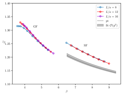
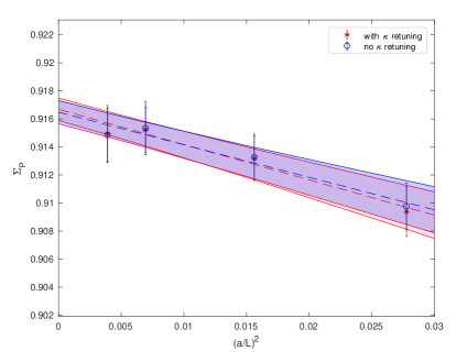
Figure 1: On the left: tuning of the boundary counterterm $z_{\rm f}$ on SF and GF ensembles. The black dotted line is the perturbative result known at $O(g_{0}^{2})$; the grey band is the result from fitting the SF data, truncated at $O(g_{0}^{2})$. The curve is discontinuous in $\beta$ as the definitions of the coupling and the gauge actions are different in the GF and SF regimes.
On the right: $\Sigma_{\rm\scriptscriptstyle P}^{\rm\scriptscriptstyle\chi SF}$ vs $(a/L)^{2}$ at $u_{\rm\scriptscriptstyle SF}$=2.012, with and without the retuning of $\kappa_{\rm c}$.

Moreover the hopping parameter $\kappa$ must be tuned to its critical value $\kappa_{\rm c}$, since $\chi$SF is a mass independent renormalisation scheme. We use the SF $\kappa_{\rm c}$ estimate of ref. [1], obtained by imposing the vanishing of the SF-PCAC mass, $m^{\rm\scriptscriptstyle SF}(g_{0}^{2},\kappa)\,\equiv\,\tilde{\partial}_{0}f_{\rm\scriptscriptstyle A}^{I}(x_{0})/2f_{\rm\scriptscriptstyle P}(x_{0})$ and then tune $z_{\rm f}$ in order to satisfy Eq.(7). This avoids having to retune $\kappa$ by imposing the vanishing of the $\chi$SF-PCAC mass, $m^{\rm\scriptscriptstyle\chi SF}(g_{0}^{2},\kappa)\,\equiv\,\tilde{\partial}_{0}g_{\rm\scriptscriptstyle A}^{ud}(x_{0})/2g_{\rm\scriptscriptstyle P}^{ud}(x_{0})$, as proposed in ref. [13]. This choice is possible because the tuning of $\kappa^{\chi\rm{SF}}$ and $z_{\rm f}$ have been shown to be weakly dependent on each other  [13], suggesting that using $\kappa_{\rm c}^{\rm{SF}}$ in place of $\kappa_{\rm c}^{\chi\rm{SF}}$ should not mistune $z_{\rm f}$. To check this explicitly we compute the step scaling function of the pseudoscalar operator at the switching scale with two $(\kappa_{\rm c},z_{\rm f})$ estimates: first we use $\kappa_{\rm c}$ of  [1] and tune $z_{\rm f}$ so that Eq.(7) is satisfied. Second we retune recursively $z_{\rm f}$ and $\kappa_{\rm c}$ until both condition (7) and $m^{\rm\scriptscriptstyle\chi SF}=0$ are satisfied. We see in Figure 1 (right panel) that the two sets of data are perfectly compatible, both at finite lattice spacing and in the continuum.

5 Running of the quark mass

We compute the running of the quark mass from hadronic scales to high-energy scales and we compare our results to those of  [1]:

$$\frac{M}{\kern 2.0pt\overline{\kern-1.0ptm\kern-1.0pt}\kern 1.0pt(\mu_{had})}=\frac{M}{\kern 2.0pt\overline{\kern-1.0ptm\kern-1.0pt}\kern 1.0pt(2^{k}\mu_{0})}\frac{\kern 2.0pt\overline{\kern-1.0ptm\kern-1.0pt}\kern 1.0pt(2^{k}\mu_{0})}{\kern 2.0pt\overline{\kern-1.0ptm\kern-1.0pt}\kern 1.0pt(\mu_{0}/2)}\frac{\kern 2.0pt\overline{\kern-1.0ptm\kern-1.0pt}\kern 1.0pt(\mu_{0}/2)}{\kern 2.0pt\overline{\kern-1.0ptm\kern-1.0pt}\kern 1.0pt(\mu_{had})}\ .$$ (8)

As in  [1], nonperturbative running factorizes into a low-energy factor computed in the GF regime (rightmost term of Eq. (8)) and a high-energy factor computed in the SF regime (central term of Eq. (8)). The leftmost factor is calculated by integrating the perturbative RGE at high energies (large $k$ value):

$$\frac{M}{\kern 2.0pt\overline{\kern-1.0ptm\kern-1.0pt}\kern 1.0pt(2^{k}\mu_{0})}=[2b_{0}\kern 1.0pt\overline{\kern-1.0ptg\kern 0.0pt}\kern 1.0pt^{2}_{{\rm SF}}(2^{k}\mu_{0})]^{-d_{0}/2b_{0}}\times\exp\Bigl{\{}-\int_{0}^{\kern 1.0pt\overline{\kern-1.0ptg\kern 0.0pt}\kern 1.0pt_{{\rm SF}}(2^{k}\mu_{0})}dx\Bigl{[}\frac{\tau(x)}{\beta(x)}-\frac{d_{0}}{b_{0}x}\Bigr{]}\Bigr{\}}\,.$$ (9)

To compute the central factor of Eq. (8), the starting point is to extract the continuum $\sigma_{\rm\scriptscriptstyle P}(u)$ from the $\Sigma_{\rm\scriptscriptstyle P}^{\rm\scriptscriptstyle\chi SF}(u,a/L)$ data (see left panel of Figure 2) through a fit constrained by the 1- and 2-loop perturbative coefficients of the continuum step scaling function.

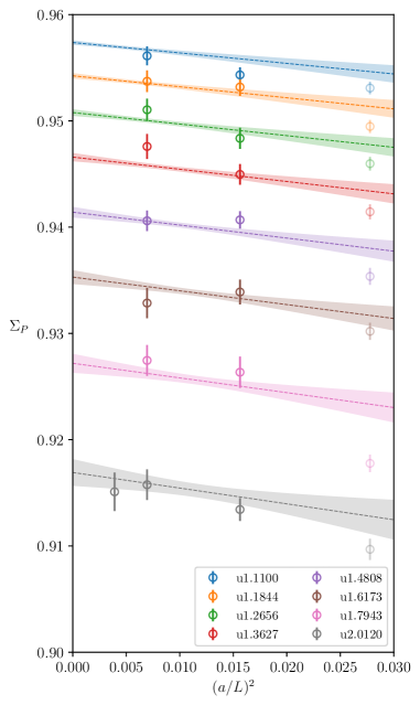
Figure 2: Left: fit to the step-scaling data $\Sigma_{\rm\scriptscriptstyle P}^{\rm\scriptscriptstyle\chi SF}(u,a/L)$ in the high-energy regime; the transparent $L/a=6$ data points are not included in the fit. The data points and the bands of the same colour are at a fixed value of the renormalised squared coupling $u$. Right: Fit to the step-scaling data $\Sigma_{\rm\scriptscriptstyle P}$ in the low-energy regime. The bands of the same colour are at a fixed value of $u$. The data points close to the bands are at approximately the same $u$.

In Figure 3 we show our result for $\sigma_{\rm\scriptscriptstyle P}(u)$ and compare it to the perturbative predictions. We see that there is a very good agreement with the 2-loop perturbative result, specific to both $\chi$SF and SF schemes.

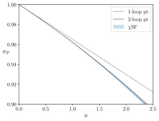
Figure 3: $\sigma_{\rm\scriptscriptstyle P}(u)$ compared with perturbation theory.

The running of quark masses from the highest energy to the switching scale is computed in terms of $\sigma_{\rm\scriptscriptstyle P}$:

$$\frac{\kern 2.0pt\overline{\kern-1.0ptm\kern-1.0pt}\kern 1.0pt(2^{k}\mu_{0})}{\kern 2.0pt\overline{\kern-1.0ptm\kern-1.0pt}\kern 1.0pt(\mu_{0}/2)}=\prod_{n=0}^{k}\sigma_{\rm\scriptscriptstyle P}(u_{n})\,,$$ (10)

where the ratio between $\mu(u_{n+1})$ and $\mu(u_{n})$ is 2, as follows from the definition of the step scaling function  (5).Having established that the result shown in Fig. 3 is a robust non-perturbative estimate of $\sigma_{\rm\scriptscriptstyle P}(u)$, even for squared couplings below the lowest simulated value $u_{\rm\scriptscriptstyle SF}$, it is possible to compute  (10) even for energy scales that lie outside our simulation range, in a region where perturbation theory can be safely applied. We have checked that our results are stable for $k\geq 5$. Our preliminary result is given for the conservative choice of $k=10$. The first two factors of  (8), i.e.  (9) and  (10), are combined to compute the running down to the switching scale, for which we find the following value:

$$\frac{M}{\kern 2.0pt\overline{\kern-1.0ptm\kern-1.0pt}\kern 1.0pt(\mu_{0}/2)}=1.7519(74)\,.$$ (11)

Alternatively we fit the $\Sigma_{\rm\scriptscriptstyle P}^{\rm\scriptscriptstyle\chi SF}(u,a/L)$ data according to the prescription $\tau$:global of ref. [1] in order to obtain directly an estimate of the anomalous dimension $\tau(u)$ in the high-energy range. Our $\tau(u)$ result and $\beta(u)$ from ref. [1] are fed into Eq. (9), written for the scale $\mu_{0}/2$ instead of $2^{k}\mu_{0}$, giving $M/\kern 2.0pt\overline{\kern-1.0ptm\kern-1.0pt}\kern 1.0pt(\mu_{0}/2)=1.7516(81)$. In a purely SF setup, ref. [1] quotes $M/\kern 2.0pt\overline{\kern-1.0ptm\kern-1.0pt}\kern 1.0pt(\mu_{0}/2)=1.7505(89)$. All three results are in excellent agreement.

In the GF regime we fit the $\Sigma_{\rm\scriptscriptstyle P}^{\rm\scriptscriptstyle\chi SF}(u,a/L)$ data (see right side of Figure 2), but we must consider that the lowest bound of the GF sector is not obtained dividing the switching scale by a power of 2. Thus we prefer to compute the running in terms of the mass anomalous dimension $\tau(\kern 1.0pt\overline{\kern-1.0ptg\kern 0.0pt}\kern 1.0pt)$, using the relation

$$\sigma_{P}(u)=\exp{\Bigl{[}-\int_{\sqrt{u}}^{\sqrt{\sigma(u)}}dg\frac{\tau(g)}{\beta(g)}\Bigr{]}}\,.$$ (12)

Our result for the running factor between the switching and the hadronic scales

$$\frac{\kern 2.0pt\overline{\kern-1.0ptm\kern-1.0pt}\kern 1.0pt(\mu_{0}/2)}{\kern 2.0pt\overline{\kern-1.0ptm\kern-1.0pt}\kern 1.0pt(\mu_{\text{had}})}=\exp{\Bigl{[}-\int_{\sqrt{\sigma(u_{0})}}^{\sqrt{u_{had}}}dg\frac{\tau(g)}{\beta(g)}\Bigr{]}}\,,$$ (13)

is

$$\frac{{\kern 2.0pt\overline{\kern-1.0ptm\kern-1.0pt}\kern 1.0pt(\mu_{0}/2)}}{\kern 2.0pt\overline{\kern-1.0ptm\kern-1.0pt}\kern 1.0pt(\mu_{\text{had}})}=0.5199(39)\,.$$ (14)

This is also in good agreement with the result of  [1]: $\kern 2.0pt\overline{\kern-1.0ptm\kern-1.0pt}\kern 1.0pt(\mu_{0}/2)/\kern 2.0pt\overline{\kern-1.0ptm\kern-1.0pt}\kern 1.0pt(\mu_{\text{had}})=0.5226(43)$. Putting everything together gives:

$$\frac{M}{\kern 2.0pt\overline{\kern-1.0ptm\kern-1.0pt}\kern 1.0pt(\mu_{\text{had}})}=0.9108(78).$$ (15)

As expected from previous results, it agrees well with its SF counterpart of ref. [1]: $M/\kern 2.0pt\overline{\kern-1.0ptm\kern-1.0pt}\kern 1.0pt(\mu_{\text{had}})=0.9148(88)$.

References

- [1] I. Campos et al. [ALPHA], Eur. Phys. J. C 78 (2018) no.5, 387 doi:10.1140/epjc/s10052-018-5870-5 [arXiv:1802.05243 [hep-lat]].
- [2] S. Sint, Nucl. Phys. B 847 (2011), 491-531 doi:10.1016/j.nuclphysb.2011.02.002 [arXiv:1008.4857 [hep-lat]].
- [3] S. Sint and B. Leder, PoS LATTICE2010 (2010), 265 doi:10.22323/1.105.0265 [arXiv:1012.2500 [hep-lat]].
- [4] P. V. Mainar, M. Dalla Brida and M. Papinutto, PoS LATTICE2015 (2016), 252 doi:10.22323/1.251.0252
- [5] I. Campos, M. Dalla Brida, G. M. de Divitiis, A. Lytle, M. Papinutto and A. Vladikas, PoS LATTICE2019 (2019), 202 doi:10.22323/1.363.0202 [arXiv:1910.01898 [hep-lat]].
- [6] M. Dalla Brida, S. Sint and P. Vilaseca, JHEP 08 (2016), 102 doi:10.1007/JHEP08(2016)102 [arXiv:1603.00046 [hep-lat]].
- [7] I. C. Plasencia, M. D. Brida, G. M. de Divitiis, A. Lytle, M. Papinutto, L. Pirelli and A. Vladikas, [arXiv:2111.15325 [hep-lat]].
- [8] M. Bruno et al. [ALPHA], Phys. Rev. Lett. 119 (2017) no.10, 102001 doi:10.1103/PhysRevLett.119.102001 [arXiv:1706.03821 [hep-lat]].
- [9] M. Dalla Brida et al. [ALPHA], Phys. Rev. Lett. 117 (2016) no.18, 182001 doi:10.1103/PhysRevLett.117.182001 [arXiv:1604.06193 [hep-ph]].
- [10] M. Dalla Brida et al. [ALPHA], Phys. Rev. D 95 (2017) no.1, 014507 doi:10.1103/PhysRevD.95.014507 [arXiv:1607.06423 [hep-lat]].
- [11] M. Luscher, R. Narayanan, P. Weisz and U. Wolff, Nucl. Phys. B 384 (1992), 168-228 doi:10.1016/0550-3213(92)90466-O [arXiv:hep-lat/9207009 [hep-lat]].
- [12] P. Fritzsch and A. Ramos, JHEP 10 (2013), 008 doi:10.1007/JHEP10(2013)008 [arXiv:1301.4388 [hep-lat]].
- [13] M. Dalla Brida, T. Korzec, S. Sint and P. Vilaseca, Eur. Phys. J. C 79 (2019) no.1, 23 doi:10.1140/epjc/s10052-018-6514-5 [arXiv:1808.09236 [hep-lat]].