Continuous Control With Ensemble Deep Deterministic Policy Gradients

Abstract

The growth of deep reinforcement learning (RL) has brought multiple exciting tools and methods to the field. This rapid expansion makes it important to understand the interplay between individual elements of the RL toolbox. We approach this task from an empirical perspective by conducting a study in the continuous control setting. We present multiple insights of fundamental nature, including: an average of multiple actors trained from the same data boosts performance; the existing methods are unstable across training runs, epochs of training, and evaluation runs; a commonly used additive action noise is not required for effective training; a strategy based on posterior sampling explores better than the approximated UCB combined with the weighted Bellman backup; the weighted Bellman backup alone cannot replace the clipped double Q-Learning; the critics’ initialization plays the major role in ensemble-based actor-critic exploration. As a conclusion, we show how existing tools can be brought together in a novel way, giving rise to the Ensemble Deep Deterministic Policy Gradients (ED2) method, to yield state-of-the-art results on continuous control tasks from OpenAI Gym MuJoCo. From the practical side, ED2 is conceptually straightforward, easy to code, and does not require knowledge outside of the existing RL toolbox.

1 Introduction

Recently, deep reinforcement learning (RL) has achieved multiple breakthroughs in a range of challenging domains (e.g. Silver et al. (2016); Berner et al. (2019); Andrychowicz et al. (2020b); Vinyals et al. (2019)). A part of this success is related to an ever-growing toolbox of tricks and methods that were observed to boost the RL algorithms’ performance (e.g. Hessel et al. (2018); Haarnoja et al. (2018b); Fujimoto et al. (2018); Wang et al. (2020); Osband et al. (2019)). This state of affairs benefits the field but also brings challenges related to often unclear interactions between the individual improvements and the credit assignment related to the overall performance of the algorithm (Andrychowicz et al., 2020a; Ilyas et al., 2020).

In this paper, we present a comprehensive empirical study of multiple tools from the RL toolbox applied to the continuous control in the OpenAI Gym MuJoCo setting. These are presented in Section 4 and Appendix B. Our insights include:

• The ensemble of actors boost the agent performance.

• The current state-of-the-art methods are unstable under several stability criteria.

• The normally distributed action noise, commonly used for exploration, can hinder training.

• The approximated posterior sampling exploration (Osband et al., 2013) outperforms approximated UCB exploration combined with weighted Bellman backup (Lee et al., 2020).

• The weighted Bellman backup (Lee et al., 2020) can not replace the clipped double Q-Learning (Fujimoto et al., 2018).

• The critics’ initialization plays a major role in ensemble-based actor-critic exploration, while the training is mostly invariant to the actors’ initialization.

To address some of the issues listed above, we introduce the Ensemble Deep Deterministic Policy Gradient (ED2) algorithm, see Section 3. ED2 brings together existing RL tools in a novel way: it is an off-policy algorithm for continuous control, which constructs an ensemble of streamlined versions of TD3 agents and achieves the state-of-the-art performance in OpenAI Gym MuJoCo, substantially improving the results on the two hardest tasks – Ant and Humanoid. Consequently, ED2 does not require knowledge outside of the existing RL toolbox, is conceptually straightforward, and easy to code.

2 Background

We model the environment as a Markov Decision Process (MDP). It is defined by the tuple $(\mathcal{S},\mathcal{A},R,P,\gamma,p_{0})$, where $\mathcal{S}$ is a continuous multi-dimensional state space, $\mathcal{A}$ denotes a continuous multi-dimensional action space, $P$ is a transition kernel, $\gamma\in[0,1)$ stands for a discount factor, $p_{0}$ refers to an initial state distribution, and $R$ is a reward function. The agent learns a policy from sequences of transitions $\tau=[(s_{t},a_{t},r_{t},s_{t+1},d)]^{T}_{t=0}$, called episodes or trajectories, where $a_{t}\sim\pi(\cdot|s_{t})$, $s_{t+1}\sim P(\cdot|s_{t},a_{t})$, $r_{t}=R(s_{t},a_{t},s_{t+1})$, $d$ is a terminal signal, and $T$ is the terminal time-step. A stochastic policy $\pi(a|s)$ maps each state to a distribution over actions. A deterministic policy $\mu:\mathcal{S}\xrightarrow{}\mathcal{A}$ assigns each state an action.

All algorithms that we consider in this paper use a different policy for collecting data (exploration) and a different policy for evaluation (exploitation). In order to keep track of the progress, the evaluation runs are performed every ten thousand environment interactions. Because of the environments’ stochasticity, we run the evaluation policy multiple times. Let $\{R_{i}\}_{i=1}^{N}$ be a set of (undiscounted) returns from $N$ evaluation episodes $\{\tau_{i}\}_{i=1}^{N}$, i.e. $R_{i}=\sum_{r_{t}\in\tau_{i}}r_{t}$. We evaluate the policy using the average test return $\bar{R}=\frac{1}{N}\sum_{i=1}^{N}R_{i}$ and the standard deviation of the test returns $\sigma=\sqrt{\frac{1}{N-1}\sum_{i=1}^{N}(R_{i}-\bar{R})^{2}}$.

We run experiments on four continuous control tasks and their variants, introduced in the appropriate sections, from the OpenAI Gym MuJoCo suite (Brockman et al., 2016). The agent observes vectors that describe the kinematic properties of the robot and its actions specify torques to be applied on the robot joints. See Appendix D for the details on the experimental setup.

3 Ensemble Deep Deterministic Policy Gradients

For completeness of exposition, we present ED2 before the experimental section. The ED2 architecture is based on an ensemble of Streamlined Off-Policy (SOP) agents (Wang et al., 2020), meaning that our agent is an ensemble of TD3-like agents (Fujimoto et al., 2018) with the action normalization and the ERE replay buffer. The pseudo-code listing can be found in Algorithm 1, while the implementation details, including a more verbose version of pseudo-code (Algorithm 3), can be found in Appendix E. In the data collection phase (Lines 2-10), ED2 selects one actor from the ensemble uniformly at random (Lines 2 and 10) and run its deterministic policy for the course of one episode (Line 5). In the evaluation phase (not shown in Algorithm 1), the evaluation policy averages all the actors’ output actions. We train the ensemble every 50 environment steps with 50 stochastic gradient descent updates (Lines 11-14). ED2 concurrently learns $K\cdot 2$ Q-functions, $Q_{\phi_{k,1}}$ and $Q_{\phi_{k,2}}$ where $k\in K$, by mean square Bellman error minimization, in almost the same way that SOP learns its two Q-functions. The only difference is that we have $K$ critic pairs that are initialized with different random weights and then trained independently with the same batches of data. Because of the different initial weights, each Q-function has a different bias in its Q-values. The $K$ actors, $\pi_{\theta_{k}}$, train maximizing their corresponding first critic, $Q_{\phi_{k,1}}$, just like SOP.

Utilizing the ensembles requires several design choices, which we summarize below. The ablation study of ED2 elements is provided in Appendix C.

Algorithm 1 ED2 - Ensemble Deep Deterministic Policy Gradients

1:Input: init. params for policy $\theta_{k}$ and Q-functions $\phi_{k,1}$, $\phi_{k,2}$, $k\in[1...K]$; replay buffer $\mathcal{D}$;

2:Sample the current policy index $c\sim\mathcal{U}([1...K])$.

3:Reset the environment and observe the state $s$.

4:repeat

5:     Execute action $a=\mu_{\theta_{c}}(s)$ $\triangleright$ $\mu$ uses the action normalization

6:     Observe and store $(s,a,r,s^{\prime},d)$ in the replay buffer $\mathcal{D}$.

7:     Set $s\leftarrow s^{\prime}$

8:     if episode is finished then

9:         Reset the environment and observe initial state $s$.

10:         Sample the current policy index $c\sim\mathcal{U}([1...K])$.      

11:     if time to update then

12:         for as many as steps done in the environment do

13:              Sample a batch of transitions $B=\{(s,a,r,s^{\prime},d)\}\subset\mathcal{D}$ $\triangleright$ uses ERE

14:              Update the parameters $\theta_{k}$, $\phi_{k,1}$ and $\phi_{k,2}$ by one gradient step.               

15:until convergence

Ensemble

Used: We train the ensemble of $5$ actors and $5$ critics; each actor learns from its own critic and the whole ensemble is trained on the same data.

Not used: We considered different actor-critic configurations, initialization schemes and relations, as well as the use of random prior networks (Osband et al., 2018), data bootstrap (Osband et al., 2016), and different ensemble sizes. We also change the SOP network sizes and training intensity instead of using the ensemble. Besides the prior networks in some special cases, these turn out to be inferior as shown in Section 4 and Appendix B.1.

Exploration

Used: We pick one actor uniformly at random to collect the data for the course of one episode. The actor is deterministic (no additive action noise is applied). These two choices ensure coherent and temporally-extended exploration similarly to Osband et al. (2016).

Not used: We tested several approaches to exploration: using the ensemble of actors, UCB (Lee et al., 2020), and adding the action noise in different proportions. These experiments are presented in Appendix B.2.

Exploitation

Used: The evaluation policy averages all the actors’ output actions to provide stable performance.

Not used: We tried picking an action with the biggest value estimate (average of the critics’ Q-functions) in evaluation (Huang et al., 2017).

Interestingly, both policies had similar results, see Appendix B.3.

Action normalization

Used: We use the action normalization introduced by Wang et al. (2020).

Not used: We experimented with the observations and rewards normalization, which turned out to be unnecessary. The experiments are presented in Appendix B.4.

Q-function updates

Used: We do $50$ SGD updates (ADAM optimizer (Kingma and Ba, 2015), MSE loss) to the actors and the critics every $50$ environment interactions, use Clipped Double Q-Learning (Fujimoto et al., 2018).

Not used: We also examined doing the updates at the end of each episode (with the proportional number of updates), using the Hubert loss, and doing weighted Bellman backups (Lee et al., 2020). However, we found them to bring no improvement to our method, as presented in Appendix B.5.

4 Experiments

In this section, we present our comprehensive study and the resulting insights. The rest of the experiments verifying that our design choices perform better than alternatives are in Appendix B. Unless stated otherwise, a solid line in the figures represents an average, while a shaded region shows a 95% bootstrap confidence interval. We used $30$ seeds for ED2 and the baselines, and $7$ seeds for the ED2 variants.

4.1 Ensemble of actors boost the agent performance

ED2 achieves state-of-the-art performance on the OpenAI Gym MuJoCo suite. Figure 1 shows the results of ED2 contrasted with three strong baselines: SUNRISE (Lee et al., 2020) – which is also the ensemble-based method – SOP (Wang et al., 2020), and SAC (Haarnoja et al., 2018b).

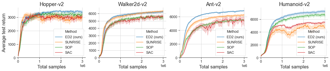
Figure 1: The average test returns across the training of ED2 and the three baselines.

Figure 2 shows ED2 with different ensemble sizes. As can be seen, the ensemble of size 5 (which we use in ED2) achieves good results, striking a balance between performance and computational overhead.

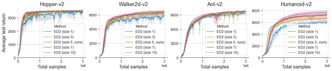
Figure 2: The average test returns across the training of ED2 with a different number of actor-critics.

4.2 The current state-of-the-art methods are unstable under several stability criteria

We consider three notions of stability: inference stability, asymptotic performance stability, and training stability. ED2 outperforms baselines in each of these notions, as discussed below. Similar metrics were also studied in Chan et al. (2020).

Inference stability

We say that an agent is inference stable if, when run multiple times, it achieves similar test performance every time. We measure inference stability using the standard deviation of test returns explained in Section 2. We found that that the existing methods train policies that are surprisingly sensitive to the randomness in the environment initial conditions. Figure 1 and Figure 3 show that ED2 successfully mitigates this problem. By the end of the training, ED2 produces results within $1\%$ of the average performance on Humanoid, while the performance of SUNRISE, SOP, and SAC may vary as much as $11\%$.

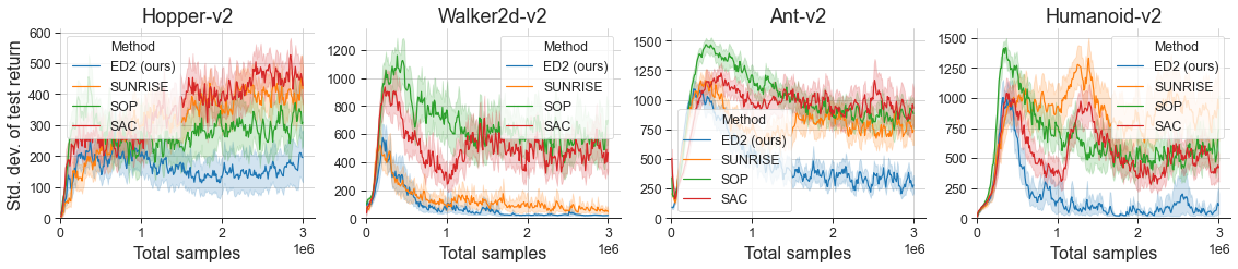
Figure 3: The standard deviation of test returns across training (lower is better), see Section 2.

Asymptotic performance stability

We say that an agent achieves asymptotic performance stability if it achieves similar test performance across multiple training runs starting from different initial networks weights. Figure 4 shows that ED2 has a significantly smaller variance than the other methods while maintaining high performance.

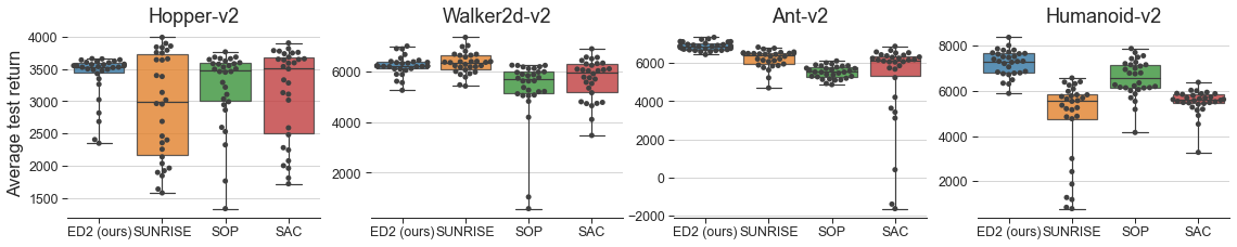
Figure 4: The dots are the average test returns after training ($3M$ samples) of each seed. The distance between each box’s top and bottom edges is the interquartile range (IQR). The whiskers spread across all values.

Training stability

We will consider training stable if performance does not severely deteriorate from one evaluation to the next. We define the root mean squared deterioration metric (RMSD) as follows:

$$\texttt{RMSD}=\sqrt{\frac{1}{M}\sum_{i=1}^{M}\Big{(}\max(\bar{R}_{i-20}-\bar{R}_{i},0)\Big{)}^{2}},$$

where $M$ is the number of the evaluation phases during training and $\bar{R}_{i}$ is the average test return at the $i$-th evaluation phase (described in Section 2). We compare returns 20 evaluation phases apart to ensure that the deterioration in performance doesn’t stem from the evaluation variance. ED2 has the lowest RMSD across all tasks, see Figure 5.

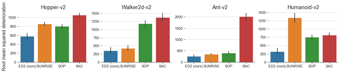
Figure 5: RMSD, the average and the 95% bootstrap confidence interval over 30 seeds.

4.3 The normally distributed action noise, commonly used for exploration, can hinder training

In this experiment, we deprive SOP of its exploration mechanism, namely additive normal action noise with the standard deviation of $0.29$, and call this variant deterministic SOP (det. SOP). The lack of the action noise, while simplifying the algorithm, causes relatively minor deterioration in the Humanoid performance, has no significant influence on the Hopper or Walker performance, and substantially improves the Ant performance, see Figure 6. This result shows that no additional exploration mechanism, often in a form of an exploration noise (Lillicrap et al., 2016; Fujimoto et al., 2018; Wang et al., 2020), is required for the diverse data collection and, in case of Ant, it even hinders training.

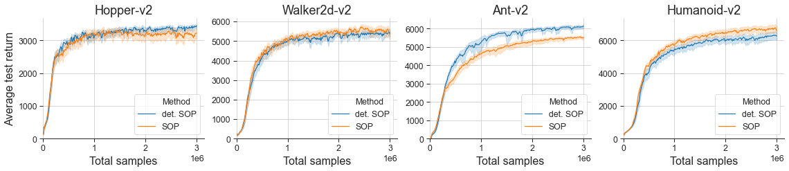
Figure 6: The average test returns across the training of SOP without and with the exploration noise. All metrics were computed over 30 seeds.

ED2 leverages this insight and constructs an ensemble of deterministic SOP agents presented in Section 3. Figure 7 shows that ED2 exhibit the same effects coming from the exploration without the action noise. In Figure 8 we present the more refined experiment where we vary the noise level. With more noise the Humanoid results get better, whereas the Ant results get much worse.

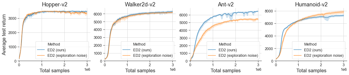
Figure 7: The average test returns across the training of ED2 with and without the exploration noise. We used Gaussian noise with the standard deviation of $0.29$, the default from Wang et al. (2020).

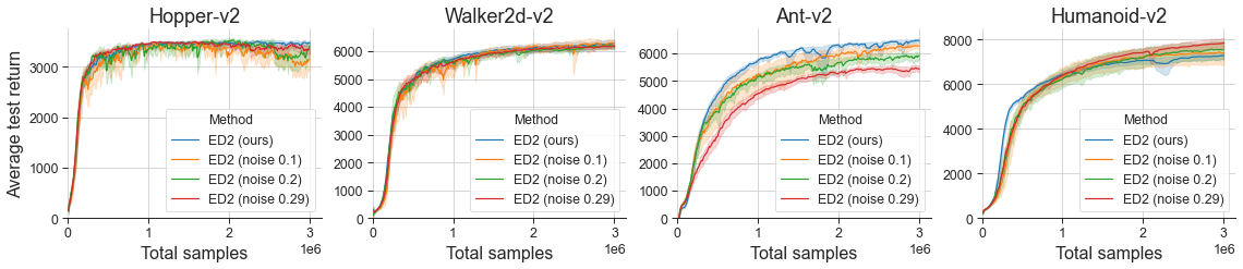
Figure 8: The average test returns across the training of ED2 with and without the exploration noise. Different noise standard deviations.

4.4 The approximated posterior sampling exploration outperforms approximated UCB exploration combined with weighted Bellman backup

The posterior sampling is proved to be theoretically superior to the OFU strategy (Osband and Van Roy, 2017). We prove this empirically for the approximate methods. ED2 uses posterior sampling exploration approximated with the bootstrap (Osband et al., 2016). SUNRISE, on the other hand, approximates the Upper Confidence Bound (UCB) exploration technique and does weighted Bellman backups (Lee et al., 2020). For the fair comparison between ED2 and SUNRISE, we substitute the SUNRISE base algorithm SAC for the SOP algorithm used by ED2. We call this variant SUNRISE-SOP.

We test both methods on the standard MuJoCo benchmarks as well as delayed (Zheng et al., 2018a) and sparse (Plappert et al., 2018) rewards variants. Both variations make the environments harder from the exploration standpoint. In the delayed version, the rewards are accumulated and returned to the agent only every 10 time-steps. In the sparse version, the reward for the forward motion is returned to the agent only after it crosses the threshold of one unit on the x-axis. For a better perspective, a fully trained Humanoid is able to move to around five units until the end of the episode. All the other reward components (living reward, control cost, and contact cost) remain unchanged. The results are presented in Table 1.

Environment	SOP	SUNRISE-SOP	ED2	Improvement over SOP	Improvement over SUNRISE-SOP
Hopper-v2	$3350$	$3083$	$3512$	$+5\%$	$+14\%$
Walker-v2	$5458$	$5730$	$6222$	$+14\%$	$+9\%$
Ant-v2	$\mathbf{5507}$	$\mathbf{771}$	$\mathbf{6862}$	$\mathbf{+25\%}$	$\mathbf{+790\%}$
Humanoid-v2	$\mathbf{6456}$	$\mathbf{5738}$	$\mathbf{7307}$	$\mathbf{+13\%}$	$\mathbf{+27\%}$
DelayedHopper-v2	$2990$	$2708$	$3315$	$+11\%$	$+22\%$
DelayedWalker-v2	$4907$	$4505$	$5940$	$+21\%$	$+32\%$
DelayedAnt-v2	$4216$	$\mathbf{1486}$	$\mathbf{3611}$	$-14\%$	$\mathbf{+43\%}$
DelayedHumanoid-v2	$\mathbf{770}$	$\mathbf{1129}$	$\mathbf{3823}$	$\mathbf{+397\%}$	$\mathbf{+239\%}$
SparseHopper-v2	$2798$	$2644$	$3397$	$+21\%$	$+29\%$
SparseWalker-v2	$4830$	$4664$	$5936$	$+23\%$	$+27\%$
SparseAnt-v2	$5573$	$\mathbf{3625}$	$\mathbf{5466}$	$-2\%$	$\mathbf{+51\%}$
SparseHumanoid-v2	$\mathbf{5433}$	$\mathbf{5225}$	$\mathbf{7438}$	$\mathbf{+37\%}$	$\mathbf{+42\%}$

Table 1: The test returns after training (3M samples) median across 30 seeds for the standard MuJoCo and 7 seeds for the delayed/sparse variants.

The performance in MuJoCo environments benefits from the ED2 approximate Bayesian posterior sampling exploration (Osband et al., 2013) in contrast to the approximated UCB in SUNRISE, which follows the OFU principle. Moreover, ED2 outperforms the non-ensemble method SOP, supporting the argument of coherent and temporally-extended exploration of ED2.

The experiment where the ED2’s exploration mechanism is replaced for UCB is in Appendix B.2. This variant also achieves worse results than ED2. The additional exploration efficiency experiment in the custom Humanoid environment, where an agent has to find and reach a goal position, is in Appendix A.

4.5 The weighted Bellman backup can not replace the clipped double Q-Learning

We applied the weighted Bellman backups proposed by Lee et al. (2020) to our method. It is suggested that the method mitigates error propagation in Q-learning by re-weighting the Bellman backup based on uncertainty estimates from an ensemble of target Q-functions (i.e. variance of predictions). Interestingly, Figure 9 does not show this positive effect on ED2.

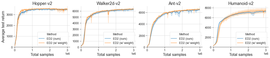
Figure 9: The average test returns across the training of our method and ED2 with the weighted Bellman backup.

Our method uses clipped double $Q$-Learning to mitigate overestimation in $Q$-functions (Fujimoto et al., 2018). We wanted to check if it is required and if it can be exchanged for the weighted Bellman backups used by Lee et al. (2020). Figure 10 shows that clipped double Q-Learning is required and that the weighted Bellman backups can not replace it.

Figure 10: The average test returns across the training of our method and ED2 without clipped double Q-Learning in two variants without and with the weighted Bellman backups.

4.6 The critics’ initialization plays a major role in ensemble-based actor-critic exploration, while the training is mostly invariant to the actors’ initialization

In this experiment, actors’ weights are initialized with the same random values (contrary to the standard case of different initialization). Moreover, we test a corresponding case with critics’ weights initialized with the same random values or simply training only a single critic.

Figure 11 indicates that the choice of actors initialization does not matter in all tasks but Humanoid. Although the average performance on Humanoid seems to be better, it is also less stable. This is quite interesting because the actors are deterministic. Therefore, the exploration must come from the fact that each actor is trained to optimize his own critic.

On the other hand, Figure 11 shows that the setup with the single critic severely impedes the agent performance. We suspect that using the single critic impairs the agent exploration capabilities as its actors’ policies, trained to maximize the same critic’s $Q$-function, become very similar.

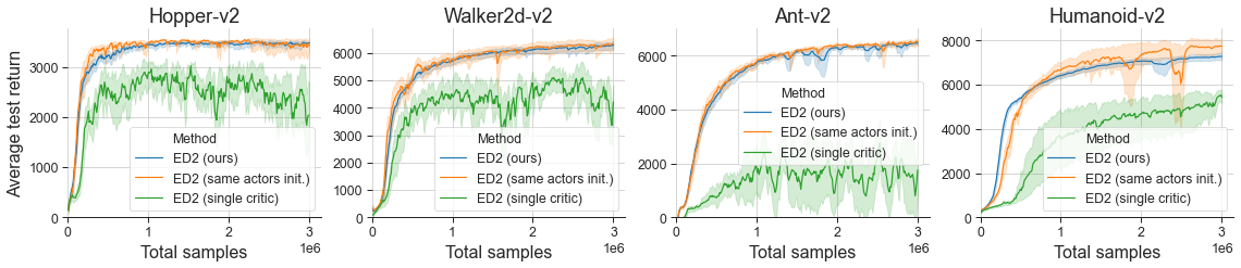
Figure 11: The average test returns across the training of ED2, ED2 with actors initialized to the same random values, and ED2 with the single critic.

5 Related work

Off-policy RL

Recently, multiple deep RL algorithms for continuous control have been proposed, e.g. DDPG (Lillicrap et al., 2016), TD3 (Fujimoto et al., 2018), SAC (Haarnoja et al., 2018b), SOP (Wang et al., 2020), SUNRISE (Lee et al., 2020). They provide a variety of methods for improving training quality, including double-Q bias reduction (van Hasselt et al., 2016), target policy smoothing or different update frequencies for actor and critic (Fujimoto et al., 2018), entropy regularization (Haarnoja et al., 2018b), action normalization (Wang et al., 2020), prioritized experience replay (Wang et al., 2020), weighted Bellman backups (Kumar et al., 2020; Lee et al., 2020), and use of ensembles (Osband et al., 2019; Lee et al., 2020; Kurutach et al., 2018; Chua et al., 2018).

Ensembles

Deep ensembles are a practical approximation of a Bayesian posterior, offering improved accuracy and uncertainty estimation (Lakshminarayanan et al., 2017; Fort et al., 2019). They inspired a variety of methods in deep RL. They are often used for temporally-extended exploration; see the next paragraph. Other than that, ensembles of different TD-learning algorithms were used to calculate better $Q$-learning targets (Chen et al., 2018). Others proposed to combine the actions and value functions of different RL algorithms (Wiering and van Hasselt, 2008) or the same algorithm with different hyper-parameters (Huang et al., 2017). For mixing the ensemble components, complex self-adaptive confidence mechanisms were proposed in Zheng et al. (2018b). Our method is simpler: it uses the same algorithm with the same hyper-parameters without any complex or learnt mixing mechanism. Lee et al. (2020) proposed a unified framework for ensemble learning in deep RL (SUNRISE) which uses bootstrap with random initialization (Osband et al., 2016) similarly to our work. We achieve better results than SUNRISE and show in Appendix B that their UCB exploration and weighted Bellman backups do not aid our algorithm performance.

Exploration

Various frameworks have been developed to balance exploration and exploitation in RL. The optimism in the face of uncertainty principle (Lai and Robbins, 1985; Bellemare et al., 2016) assigns an overly optimistic value to each state-action pair, usually in the form of an exploration bonus reward, to promote visiting unseen areas of the environment. The maximum entropy method (Haarnoja et al., 2018a) encourages the policy to be stochastic, hence boosting exploration. In the parameter space approach (Plappert et al., 2018; Fortunato et al., 2018), noise is added to the network weights, which can lead to temporally-extended exploration and a richer set of behaviours. Posterior sampling (Strens, 2000; Osband et al., 2016; 2018) methods have similar motivations. They stem from the Bayesian perspective and rely on selecting the maximizing action among sampled and statistically plausible set of action values. The ensemble approach (Lowrey et al., 2018; Miłoś et al., 2019; Lee et al., 2020) trains multiple versions of the agent, which yields a diverse set of behaviours and can be viewed as an instance of posterior sampling RL.

6 Conclusions

We conduct a comprehensive empirical analysis of multiple tools from the RL toolbox applied to the continuous control in the OpenAI Gym MuJoCo setting. We believe that the findings can be useful to RL researchers. Additionally, we propose Ensemble Deep Deterministic Policy Gradients (ED2), an ensemble-based off-policy RL algorithm, which achieves state-of-the-art performance and addresses several issues found during the aforementioned study.

Reproducibility Statement

We have made a significant effort to make our results reproducible. We use 30 random seeds, which is above the currently popular choice in the field (up to 5 seeds). Furthermore, we systematically explain our design choices in Section 3 and we provide a detailed pseudo-code of our method in Algorithm 3 in the Appendix B. Additionally, we open-sourced the code for the project together with examples of how to reproduce the main experiments. The implementation details are explained in Appendix E and extensive information about the experimental setup is given in Appendix D.

Appendix A Exploration efficiency in the custom Humanoid environment

To check the exploration capabilities of our method, we constructed two environments based on Humanoid where the goal is not only to move forward as fast as possible but to find and get to the specific region. The environments are described in Figure 13.

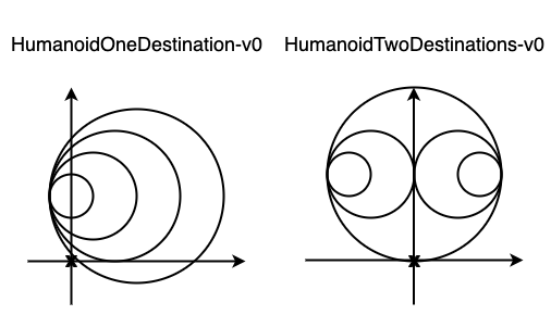
Figure 12: This is a top-down view. Humanoid starts at the origin (marked ’x’). The reward in each time-step is equal to the number of circles for which the agent is inside. Being in the most nested circle (or either of two) solves the task.

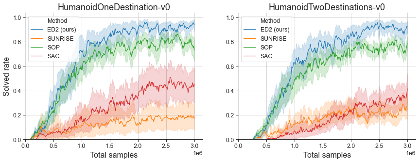
Figure 13: The fraction of episodes in which the task is finished for ED2 and two baselines. The average and the 95% bootstrap confidence interval over 20 seeds.

Because the Humanoid initial state is slightly perturbed every run, we compare solved rates over multiple runs, see details in Appendix D. Figure 13 compares the solved rates of our method and the three baselines. Our method outperforms the baselines. For this experiment, our method uses the prior networks [Osband et al., 2018].

Appendix B Design choices

In this section, we summarize the empirical evaluation of various design choices grouped by topics related to an ensemble of agents (B.1), exploration (B.2), exploitation (B.3), normalization (B.4), and $Q$-function updates (B.5). In the plots, a solid line and a shaded region represent an average and a 95% bootstrap confidence interval over $30$ seeds in case of ED2 (ours) and $7$ seeds otherwise. All of these experiments test ED2 presented in Section 3 with Algorithm 2 used for evaluation (the ensemble critic variant). We call Algorithm 2 a ’vote policy’.

Algorithm 2 Vote policy

1:Input: ensemble size $K$; policy $\theta_{k}$ and $Q$-function $\phi_{k,1}$ parameters where $k\in[1,\ldots,K]$; max action scale $M$;

2:function vote_policy($s$, $c$)

$$a_{k}=M\tanh\left(\mu_{\theta_{k}}(s)\right)\;\;\;\text{for }k\in[1,\ldots,K]$$ (1)

3:     if use arbitrary critic then

$$q_{k}=Q_{\phi_{c,1}}(s,a_{k})\;\;\;\text{for }k\in[1,\ldots,K]$$ (2)

4:     else use ensemble critic

$$q_{k}=\frac{1}{K}\sum_{i\in[1...K]}Q_{\phi_{i,1}}(s,a_{k})\;\;\;\text{for }k\in[1,\ldots,K]$$ (3)

     

5:     return $a_{k}$ for $k=\operatorname*{argmax}_{k}{q_{k}}$

B.1 Ensemble

Prior networks

We tested if our algorithm can benefit from prior networks [Osband et al., 2018]. It turned out that the results are very similar on OpenAI Gym MuJoCo tasks, see Figure 14. However, the prior networks are useful on our crafted hard-exploration Humanoid environments, see Figure 15.

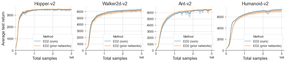
Figure 14: The average test returns across the training of ED2 without (ours) and with prior networks.

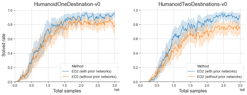
Figure 15: The average test returns across the training of ED2 without (ours) and with prior networks.

Moreover, we tested if the deterministic SOP variant can benefit from prior networks. It turned out that the results are very similar or worse, see Figure 16.

Figure 16: The average test returns across the training of SOP and SOP without the exploration noise in two variants: without and with the prior network. All metrics were computed over 30 seeds.

Ensemble size

Figure 17 shows ED2 with different ensemble sizes. As can be seen, the ensemble of size 5 (which we use in ED2) achieves good results, striking a balance between performance and computational overhead.

Figure 17: The average test returns across the training of ED2 with a different number of actor-critics.

Data bootstrap

Osband et al. [2016] and Lee et al. [2020] remark that training an ensemble of agents using the same training data but with different initialization achieves, in most cases, better performance than applying different training samples to each agent. We confirm this observation in Figure 18. Data bootstrap assigned each transition to each agent in the ensemble with 50% probability.

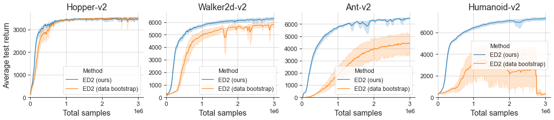
Figure 18: The average test returns across the training of ED2 without (ours) and with data bootstrap.

SOP bigger networks and training intensity

We checked if simply training SOP with bigger networks or with higher training intensity (a number of updates made for each collected transition) can get it close to the ED2 results. Figure 19 compares ED2 to SOP with different network sizes, while Figure 20 compares ED2 to SOP with one or five updates per environment step. It turns out that bigger networks or higher training intensity does not improve SOP performance.

Figure 19: The average test returns across the training of ED2 and SOP with different network sizes.

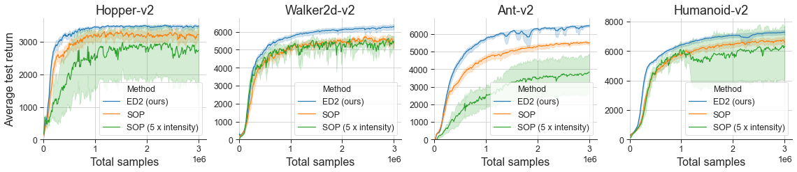
Figure 20: The average test returns across the training of ED2 and SOP with one or five updates for every step in an environment.

B.2 Exploration

Vote policy

In this experiment, we used the so-called "vote policy" described in Algorithm 2. We use it for action selection in step 6 of Algorithm 3 in two variations: (1) where the random critic, chosen for the duration of one episode, evaluates each actor’s action or (2) with the full ensemble of critics for actors actions evaluation. Figure 21 shows that the arbitrary critic is not much different from our method. However, in the case of the ensemble critic, we observe a significant performance drop suggesting deficient exploration.

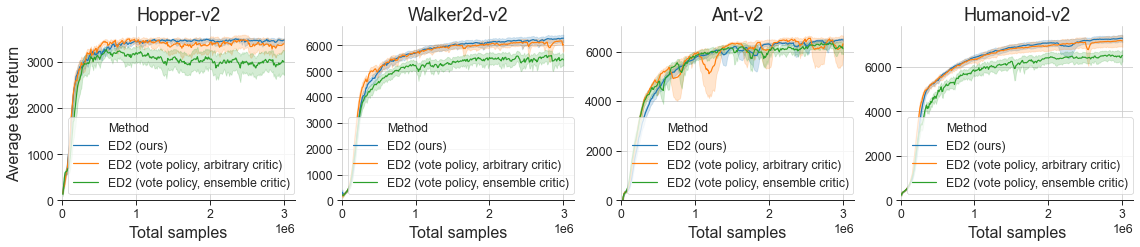
Figure 21: The average test returns across the training of ED2 with and without the vote policy for exploration.

UCB

We tested the UCB exploration method from Lee et al. [2020]. This method defines an upper-confidence bound (UCB) based on the mean and variance of Q-functions in an ensemble and selects actions with the highest UCB for efficient exploration. Figure 22 shows that the UCB exploration method makes the results of our algorithm worse.

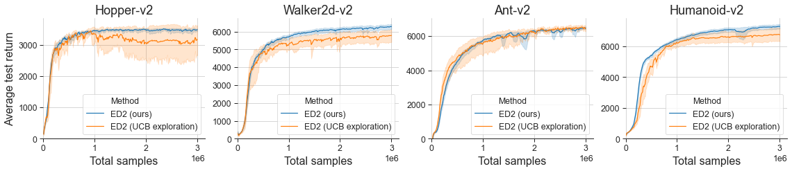
Figure 22: The average test returns across the training of our method and ED2 with the UCB exploration.

Gaussian noise

While our method uses ensemble-based temporally coherent exploration, the most popular choice of exploration is injecting i.i.d. noise [Fujimoto et al., 2018, Wang et al., 2020]. We evaluate if these two approaches can be used together. We used Gaussian noise with the standard deviation of $0.29$, it is the default value in Wang et al. [2020]. We found that the effects are task-specific, barely visible for Hopper and Walker, positive in the case of Humanoid, and negative for Ant – see Figure 23. In a more refined experiment, we varied the noise level. With more noise the Humanoid results are better, whereas the And results are worse – see Figure 24.

Figure 23: The average test returns across the training of ED2 with and without the additive Gaussian noise for exploration.

Figure 24: The average test returns across the training of ED2 with and without the additive Gaussian noise for exploration. Different noise standard deviations.

B.3 Exploitation

We used the vote policy, see Algorithm 2, as the evaluation policy in step 22 of Algorithm 3. Figure 25 shows that the vote policy does worse on the OpenAI Gym MuJoCo tasks. However, on our custom Humanoid tasks introduced in Section 4, it improves our agent performance – see Figure 26.

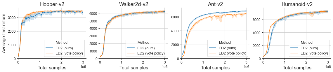
Figure 25: The average test returns across the training of our method and ED2 with the vote policy for evaluation.

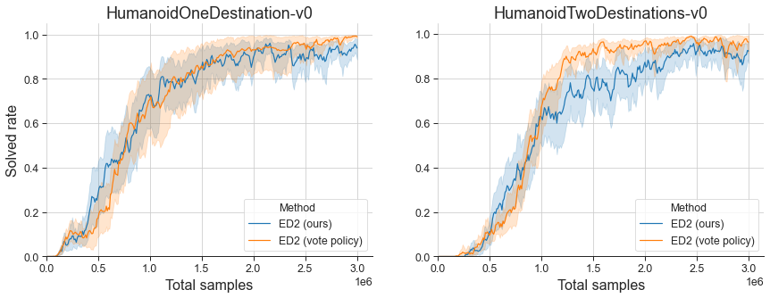
Figure 26: The average test returns across the training of our method and ED2 with the vote policy for evaluation.

B.4 Normalization

We validated if rewards or observations normalization [Andrychowicz et al., 2020a] help our method. In both cases, we keep the empirical mean and standard deviation of each reward/observation coordinate, based on all rewards/observations seen so far, and normalize rewards/observations by subtracting the empirical mean and dividing by the standard deviation. It turned out that only the observations normalization significantly helps the agent on Humanoid, see Figures 27 and 28. The action normalization influence is tested in Appendix C.

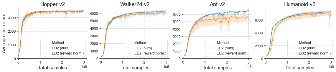
Figure 27: The average test returns across the training of our method and ED2 with the rewards normalization.

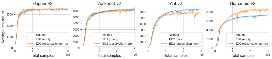
Figure 28: The average test returns across the training of our method and ED2 with the observations normalization.

B.5 $Q$-function updates

Huber loss

We tried using the Huber loss for the $Q$-function training. It makes the results on all tasks worse, see Figure 29.

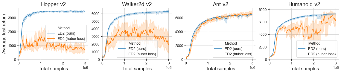
Figure 29: The average test returns across the training of our method and ED2 with the Huber loss.

Appendix C Ablation study

In this section, we ablate the ED2 components to see their impact on performance and stability. We start with the ensemble exploration and exploitation and then move on to the action normalization and the ERE replay buffer. In all plots, a solid line and a shaded region represent an average and a 95% bootstrap confidence interval over $30$ seeds in all but action normalization and ERE replay buffer experiments, where we run $7$ seeds.

Exploration & Exploitation

In the first experiment we wanted to isolate the effect of ensemble-based temporally coherent exploration on the performance and stability of ED2. Figures 30-33 compare the performance and stability of ED2 and one baseline, SOP, to ED2 with the single actor (the first one) used for evaluation in step 22 of Algorithm 3. It is worth noting that the action selection during the data collection, step 6 in Algorithm 3, is left unchanged – the ensemble of actors is used for exploration and each actor is trained on all the data. This should isolate the effect of exploration on the test performance of every actor. The results show that the performance improvement and stability of ED2 does not come solely from the efficient exploration. ED2 ablation performs comparably to the baseline and is even less stable.

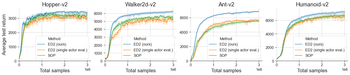
Figure 30: The average test returns across the training of ED2, ED2 with the single actor for exploitation, and the baseline.

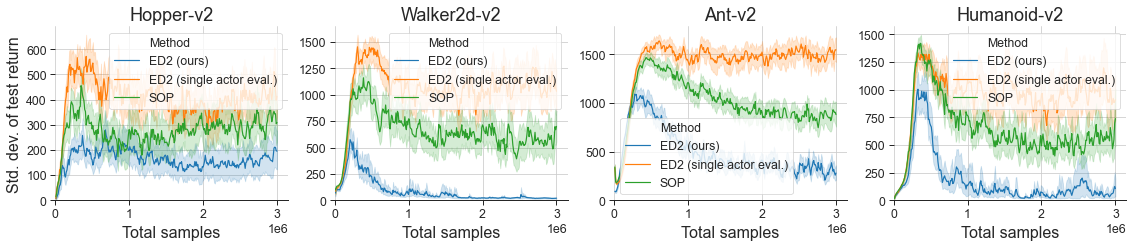
Figure 31: The standard deviation of test returns across the training of ED2, ED2 with the single actor for exploitation, and the baseline.

Figure 32: The dots are the average test returns after training ($3M$ samples) of each seed of ED2, ED2 with the single actor for exploitation, and the baseline. The distance between each box’s top and bottom edges is the interquartile range (IQR). The whiskers spread across all values.

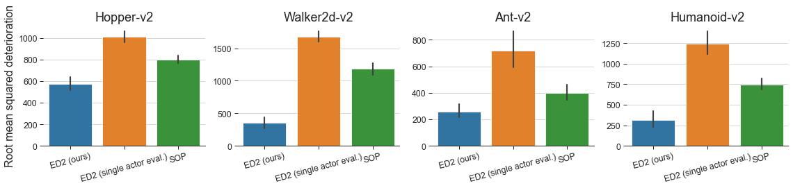
Figure 33: RMSD of ED2, ED2 with the single actor for exploitation, and the baseline – the average and the 95% bootstrap confidence interval over 30 seeds.

In the next experiment, we wanted to check if the ensemble evaluation is all we need in that event. Figure 34 compares the performance of ED2 and one baseline, SOP, to ED2 with the single actor (the first one) used for the data collection in step 6 of Algorithm 3. The action selection during the evaluation, step 22 in Algorithm 3, is left unchanged – the ensemble of actors is trained on the data collected only by one of the actors. We add Gaussian noise to the single actor’s actions for exploration as described in Appendix B.2. The results show that the ensemble actor test performance collapses, possibly because of training on the out of distribution data. This implies that the ensemble of actors, used for evaluation, improves the test performance and stability. However, it is required that the same ensemble of actors is also used for exploration, during the data collection.

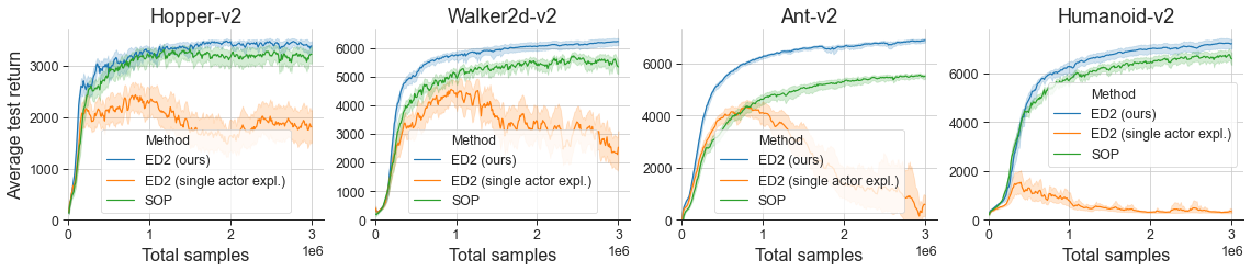
Figure 34: The average test returns across the training of ED2, ED2 with the single actor for exploration, and the baseline.

Action normalization

The implementation details of the action normalization are described in Appendix E. Figure 35 shows that the action normalization is especially required on the Ant and Humanoid environments, while not disrupting the training on the other tasks.

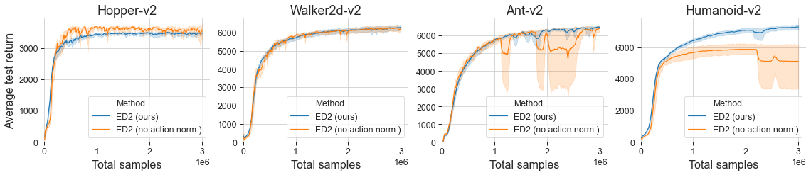
Figure 35: The average test returns across the training of ED2 with and without the action normalization.

ERE replay buffer

The implementation details of the ERE replay buffer are described in Appendix E. In Figure 36 we observe that it improves the final performance of ED2 on all tasks, especially on Walker2d and Humanoid.

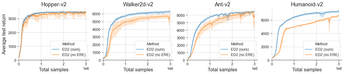
Figure 36: The average test returns across the training of ED2 with and without the ERE replay buffer.

Appendix D Experimental setup

Plots

In all evaluations, we used 30 evaluation episodes to better access the average performance of each policy, as described in Section 2. For a more pleasant look and easier visual assessment, we smoothed the lines using an exponential moving average with a smoothing factor equal $0.4$.

OpenAI Gym MuJoCo

In MuJoCo environments, presented in Figure 37, a state is defined by $(x,y,z)$ position and velocity of the robot’s root, and angular position and velocity of each of its joints. The observation holds almost all information from the state except the x and y position of the robot’s root. The action is a torque that should be applied to each joint of the robot. Sizes of those spaces for each environment are summarised in Table 2.

MuJoCo is a deterministic physics engine thus all simulations conducted inside it are deterministic. This includes simulations of our environments. However, to simplify the process of data gathering and to counteract over-fitting the authors of OpenAI Gym decided to introduce some stochasticity. Each episode starts from a slightly different state - initial positions and velocities are perturbed with random noise (uniform or normal depending on the particular environment).

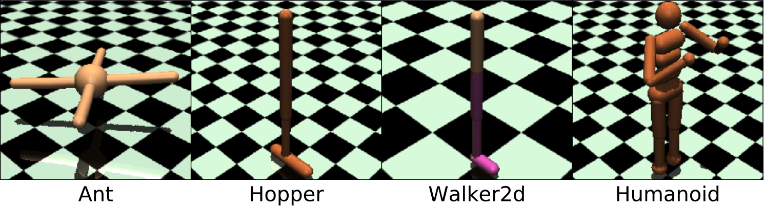
Figure 37: The OpenAI Gym MuJoCo tasks we benchmark out method on.

Environment name	Action space size	Observation space size
Hopper-v2	3	11
Walker2d-v2	6	17
Ant-v2	8	111
Humanoid-v2	17	376

Table 2: Action and observation space sizes for used environments.

Appendix E Implementation details

Algorithm 3 ED2 - Ensemble Deep Deterministic Policy Gradients

1:Input: ensemble size $K$; init. policy $\theta_{k}$ and $Q$-functions $\phi_{k,1}$, $\phi_{k,2}$ param. where $k\in[1,\ldots,K]$; replay buffer $\mathcal{D}$; max action scale $M$; target smoothing std. dev. $\sigma$; interpolation factor $\rho$;

2:Set the target parameters $\bar{\phi}_{k,1}\leftarrow\phi_{k,1}$, $\bar{\phi}_{k,2}\leftarrow\phi_{k,2}$

3:Sample the current policy index $c\sim\mathcal{U}([1,\ldots,K])$.

4:Reset the environment and observe the state $s$.

5:repeat

6:     Execute action $a=M\tanh\left(\mu_{\theta_{c}}(s)\right)$ $\triangleright$ $\mu$ uses the action normalization

7:     Observe and store $(s,a,r,s^{\prime},d)$ in the replay buffer $\mathcal{D}$.

8:     Set $s\leftarrow s^{\prime}$

9:     if episode is finished then

10:         Reset the environment and observe initial state $s$.

11:         Sample the current policy index $c\sim\mathcal{U}([1,\ldots,K])$.      

12:     if time to update then

13:         for as many as steps done in the environment do

14:              Sample a batch of transitions $B=\{(s,a,r,s^{\prime},d)\}\subset\mathcal{D}$ $\triangleright$ uses ERE

15:              Compute targets

$$y_{k}(r,s^{\prime},d) =r+\gamma(1-d)\min_{i=1,2}Q_{\bar{\phi}_{k,i}}(s^{\prime},a^{\prime}_{k})$$

$$a^{\prime}_{k} =M\tanh\left(\mu_{\theta_{k}}(s^{\prime})+\epsilon\right),\epsilon\sim\mathcal{N}(0,\sigma)$$

16:              Update the $Q$-functions by one step of gradient descent using

$$\nabla_{\phi_{k,i}}\frac{1}{|B|\cdot K}\sum_{(s,a,r,s^{\prime},d)\in B}\left(Q_{\phi_{k,i}}(s,a)-y_{k}(r,s^{\prime},d)\right)^{2}\;\;\;\text{for }i\in\{1,2\},k\in[1,\ldots,K]$$

17:              Update the policies by one step of gradient ascent using

$$\nabla_{\theta_{k}}\frac{1}{|B|\cdot K}\sum_{s\in B}Q_{\phi_{k,1}}(s,\mu_{\theta_{k}}(s))\;\;\;\text{for }k\in[1,\ldots,K]$$

18:              Update target parameters with

$$\bar{\phi}_{k,i}\leftarrow\rho\bar{\phi}_{k,i}+(1-\rho)\phi_{k,i}\;\;\;\text{for }i\in\{1,2\},k\in[1,\ldots,K]$$

              

19:     if time to evaluate then

20:         for specified number of evaluation runs do

21:              Reset the environment and observe the state $s$.

22:              Execute policy $a=\frac{1}{K}\sum_{i=1}^{K}M\tanh\left(\mu_{\theta_{i}}(s)\right)$ until the terminal state.

23:              Record and log the return.               

24:until convergence

Architecture and hyper-parameters

In our experiments, we use deep neural networks with two hidden layers, each of them with 256 units. All of the networks use ReLU as an activation, except on the final output layer, where the activation used varies depending on the model: critic networks use no activation, while actor networks use $tanh()$ multiplied by the max action scale. Table 3 shows the hyper-parameters used for the tested algorithms.

[b] Parameter SAC SOP SUNRISE ED2 discounting $\gamma$ $0.99$ $0.99$ $0.99$ $0.99$ optimizer Adam Adam Adam Adam learning rate $10^{-3}$ $10^{-4}$ $10^{-3}$ $10^{-4}$ replay buffer size $10^{6}$ $10^{6}$ $10^{6}$ $10^{6}$ batch size $256$ $256$ $256$ $256$ ensemble size - - $5$ $5$ entropy coefficient $\alpha$ $0.2$ - $0.2$ - update interval ¹ $50$ $50$ $50$ $50$ $\eta_{0}$ (ERE) - $0.995$ - $0.995$

• Number of environment interactions between updates.

Table 3: Default values of hyper-parameters were used in our experiments.

Action normalization

Our algorithm employs action normalization proposed by Wang et al. [2020]. It means that before applying the squashing function (e.g. $tanh()$), the outputs of each actor network are normalized in the following way: let $\mu=(\mu_{1},\dots,\mu_{A})$ be the output of the actor’s network and let $G=\sum_{i=1}^{A}|\mu_{i}|/A$ be the average magnitude of this output, where $A$ is the action’s dimensionality. If $G>1$ then we normalize the output by setting $\mu_{i}$ to $\mu_{i}/G$ for all $i=1,\dots,A$. Otherwise, we leave the output unchanged. Each actor’s outputs are normalized independently from other actors in the ensemble.

Emphasizing Recent Experience

We implement the Emphasizing Recent Experience (ERE) mechanism from Wang et al. [2020]. ERE samples non-uniformly from the most recent experiences stored in the replay buffer. Let $B$ be the number of mini-batch updates and $|\mathcal{D}|$ be the size of the replay buffer. When performing the gradient updates, we sample from the most recent $c_{b}$ data points stored in the replay buffer, where $c_{b}=|\mathcal{D}|\cdot\eta^{b\frac{1000}{B}}$ for $b=1,\dots,B$.

The hyper-parameter $\eta$ starts off with a set value of $\eta_{0}$ and is later adapted based on the improvements in the agent training performance. Let $I_{recent}$ be the improvement in terms of training episode returns made over the last $|\mathcal{D}|/2$ time-steps and $I_{max}$ be the maximum of such improvements over the course of the training. We adapt $\eta$ according to the formula:

$$\eta=\eta_{0}\cdot\frac{I_{recent}}{I_{max}}+1-\frac{I_{recent}}{I_{max}}$$

Our implementation uses the exponentially weighted moving average to store the value of $I_{recent}$. More concretely, we define $I_{recent}$ based on two additional parameters $R_{recent}$ and $R_{prev}$ so that $I_{recent}=R_{recent}-R_{prev}$. Those parameters are then updated whenever we receive a new training episode return $ep\_ret$:

$$R_{recent} =\lambda_{recent}\cdot ep\_ret+(1-\lambda_{recent})\cdot R_{recent}$$

$$R_{prev} =\lambda_{prev}\cdot ep\_ret+(1-\lambda_{prev})\cdot R_{prev}$$

where $\lambda_{prev}=T/\lfloor\frac{|\mathcal{D}|}{2}\rfloor$, $\lambda_{recent}=10\cdot\lambda_{prev}$ and $T$ is the maximum length of an episode.

Hardware

During the training of our models, we employ only CPUs using a cluster where each node has $28$ available cores of $2.6$ GHz, alongside at least $64$ GB of memory. The running time of a typical experiment did not exceed 24 hours.

References

- Achiam (2018) Joshua Achiam. Spinning Up in Deep Reinforcement Learning. GitHub repository, 2018.
- Andrychowicz et al. (2020a) Marcin Andrychowicz, Anton Raichuk, Piotr Stanczyk, Manu Orsini, Sertan Girgin, Raphael Marinier, Léonard Hussenot, Matthieu Geist, Olivier Pietquin, Marcin Michalski, Sylvain Gelly, and Olivier Bachem. What Matters in On-Policy Reinforcement Learning? A Large-Scale Empirical Study, 2020a. ISSN 23318422.
- Andrychowicz et al. (2020b) OpenAI: Marcin Andrychowicz, Bowen Baker, Maciek Chociej, Rafal Jozefowicz, Bob McGrew, Jakub Pachocki, Arthur Petron, Matthias Plappert, Glenn Powell, Alex Ray, et al. Learning dexterous in-hand manipulation. The International Journal of Robotics Research, 39(1):3–20, 2020b.
- Bellemare et al. (2016) Marc G. Bellemare, Sriram Srinivasan, Georg Ostrovski, Tom Schaul, David Saxton, and Rémi Munos. Unifying count-based exploration and intrinsic motivation. In Daniel D. Lee, Masashi Sugiyama, Ulrike von Luxburg, Isabelle Guyon, and Roman Garnett, editors, Advances in Neural Information Processing Systems 29: Annual Conference on Neural Information Processing Systems 2016, December 5-10, 2016, Barcelona, Spain, pages 1471–1479, 2016. URL https://proceedings.neurips.cc/paper/2016/hash/afda332245e2af431fb7b672a68b659d-Abstract.html.
- Berner et al. (2019) Christopher Berner, Greg Brockman, Brooke Chan, Vicki Cheung, Przemysław Dębiak, Christy Dennison, David Farhi, Quirin Fischer, Shariq Hashme, Chris Hesse, et al. Dota 2 with large scale deep reinforcement learning. arXiv preprint arXiv:1912.06680, 2019.
- Brockman et al. (2016) Greg Brockman, Vicki Cheung, Ludwig Pettersson, Jonas Schneider, John Schulman, Jie Tang, and Wojciech Zaremba. Openai gym, 2016.
- Chan et al. (2020) Stephanie C. Y. Chan, Samuel Fishman, Anoop Korattikara, John Canny, and Sergio Guadarrama. Measuring the Reliability of Reinforcement Learning Algorithms. In 8th International Conference on Learning Representations, ICLR 2020, Addis Ababa, Ethiopia, April 26-30, 2020. OpenReview.net, 2020.
- Chen et al. (2018) Xi Liang Chen, Lei Cao, Chen Xi Li, Zhi Xiong Xu, and Jun Lai. Ensemble Network Architecture for Deep Reinforcement Learning. Mathematical Problems in Engineering, 2018. ISSN 15635147. doi: 10.1155/2018/2129393.
- Chua et al. (2018) Kurtland Chua, Roberto Calandra, Rowan McAllister, and Sergey Levine. Deep reinforcement learning in a handful of trials using probabilistic dynamics models. In NeurIPS 2018, pages 4759–4770, 2018.
- Fort et al. (2019) Stanislav Fort, Huiyi Hu, and Balaji Lakshminarayanan. Deep ensembles: A loss landscape perspective. CoRR, abs/1912.02757, 2019. URL http://arxiv.org/abs/1912.02757.
- Fortunato et al. (2018) Meire Fortunato, Mohammad Gheshlaghi Azar, Bilal Piot, Jacob Menick, Matteo Hessel, Ian Osband, Alex Graves, Vlad Mnih, Remi Munos, Demis Hassabis, Olivier Pietquin, Charles Blundell, and Shane Legg. Noisy networks for exploration. In 6th International Conference on Learning Representations, ICLR 2018 - Conference Track Proceedings, 2018.
- Fujimoto et al. (2018) Scott Fujimoto, Herke van Hoof, and David Meger. Addressing function approximation error in actor-critic methods. In Jennifer G. Dy and Andreas Krause, editors, Proceedings of the 35th International Conference on Machine Learning, ICML 2018, Stockholmsmässan, Stockholm, Sweden, July 10-15, 2018, volume 80 of Proceedings of Machine Learning Research, pages 1582–1591. PMLR, 2018. URL http://proceedings.mlr.press/v80/fujimoto18a.html.
- Haarnoja et al. (2018a) Tuomas Haarnoja, Aurick Zhou, Pieter Abbeel, and Sergey Levine. Soft actor-critic: Off-policy maximum entropy deep reinforcement learning with a stochastic actor. In 35th International Conference on Machine Learning, ICML 2018, 2018a. ISBN 9781510867963.
- Haarnoja et al. (2018b) Tuomas Haarnoja, Aurick Zhou, Kristian Hartikainen, George Tucker, Sehoon Ha, Jie Tan, Vikash Kumar, Henry Zhu, Abhishek Gupta, Pieter Abbeel, and Sergey Levine. Soft actor-critic algorithms and applications. CoRR, abs/1812.05905, 2018b. URL http://arxiv.org/abs/1812.05905.
- Hessel et al. (2018) Matteo Hessel, Joseph Modayil, Hado Van Hasselt, Tom Schaul, Georg Ostrovski, Will Dabney, Dan Horgan, Bilal Piot, Mohammad Azar, and David Silver. Rainbow: Combining improvements in deep reinforcement learning. In 32nd AAAI Conference on Artificial Intelligence, AAAI 2018, pages 3215–3222, oct 2018. ISBN 9781577358008. URL http://arxiv.org/abs/1710.02298.
- Huang et al. (2017) Zhewei Huang, Shuchang Zhou, Bo Er Zhuang, and Xinyu Zhou. Learning to run with actor-critic ensemble, 2017. ISSN 23318422.
- Ilyas et al. (2020) Andrew Ilyas, Logan Engstrom, Shibani Santurkar, Dimitris Tsipras, Firdaus Janoos, Larry Rudolph, and Aleksander Madry. A closer look at deep policy gradients. In 8th International Conference on Learning Representations, ICLR 2020, Addis Ababa, Ethiopia, April 26-30, 2020. OpenReview.net, 2020. URL https://openreview.net/forum?id=ryxdEkHtPS.
- Kingma and Ba (2015) Diederik P. Kingma and Jimmy Ba. Adam: A method for stochastic optimization. In Yoshua Bengio and Yann LeCun, editors, 3rd International Conference on Learning Representations, ICLR 2015, San Diego, CA, USA, May 7-9, 2015, Conference Track Proceedings, 2015. URL http://arxiv.org/abs/1412.6980.
- Kumar et al. (2020) Aviral Kumar, Abhishek Gupta, and Sergey Levine. Discor: Corrective feedback in reinforcement learning via distribution correction. In Hugo Larochelle, Marc’Aurelio Ranzato, Raia Hadsell, Maria-Florina Balcan, and Hsuan-Tien Lin, editors, Advances in Neural Information Processing Systems 33: Annual Conference on Neural Information Processing Systems 2020, NeurIPS 2020, December 6-12, 2020, virtual, 2020. URL https://proceedings.neurips.cc/paper/2020/hash/d7f426ccbc6db7e235c57958c21c5dfa-Abstract.html.
- Kurutach et al. (2018) Thanard Kurutach, Ignasi Clavera, Yan Duan, Aviv Tamar, and Pieter Abbeel. Model-ensemble trust-region policy optimization. In 6th International Conference on Learning Representations, ICLR 2018, Vancouver, BC, Canada, April 30 - May 3, 2018, Conference Track Proceedings. OpenReview.net, 2018. URL https://openreview.net/forum?id=SJJinbWRZ.
- Lai and Robbins (1985) Tze Leung Lai and Herbert Robbins. Asymptotically efficient adaptive allocation rules. Advances in applied mathematics, 6(1):4–22, 1985.
- Lakshminarayanan et al. (2017) Balaji Lakshminarayanan, Alexander Pritzel, and Charles Blundell. Simple and scalable predictive uncertainty estimation using deep ensembles. In NIPS 2017, 2017.
- Lee et al. (2020) Kimin Lee, Michael Laskin, Aravind Srinivas, and Pieter Abbeel. SUNRISE: A Simple Unified Framework for Ensemble Learning in Deep Reinforcement Learning, 2020. ISSN 23318422.
- Lillicrap et al. (2016) Timothy P. Lillicrap, Jonathan J. Hunt, Alexander Pritzel, Nicolas Heess, Tom Erez, Yuval Tassa, David Silver, and Daan Wierstra. Continuous control with deep reinforcement learning. In Yoshua Bengio and Yann LeCun, editors, 4th International Conference on Learning Representations, ICLR 2016, San Juan, Puerto Rico, May 2-4, 2016, Conference Track Proceedings, 2016. URL http://arxiv.org/abs/1509.02971.
- Lowrey et al. (2018) Kendall Lowrey, Aravind Rajeswaran, Sham Kakade, Emanuel Todorov, and Igor Mordatch. Plan online, learn offline: Efficient learning and exploration via model-based control. CoRR, abs/1811.01848, 2018.
- Miłoś et al. (2019) Piotr Miłoś, Łukasz Kuciński, Konrad Czechowski, Piotr Kozakowski, and Maciek Klimek. Uncertainty-sensitive learning and planning with ensembles. arXiv preprint arXiv:1912.09996, 2019.
- Osband and Van Roy (2017) Ian Osband and Benjamin Van Roy. Why is posterior sampling better than optimism for reinforcement learning? In 34th International Conference on Machine Learning, ICML 2017, 2017. ISBN 9781510855144.
- Osband et al. (2013) Ian Osband, Benjamin Van Roy, and Daniel Russo. (More) efficient reinforcement learning via posterior sampling. In Advances in Neural Information Processing Systems, 2013.
- Osband et al. (2016) Ian Osband, Charles Blundell, Alexander Pritzel, and Benjamin Van Roy. Deep exploration via bootstrapped DQN. In Advances in Neural Information Processing Systems, 2016.
- Osband et al. (2018) Ian Osband, John Aslanides, and Albin Cassirer. Randomized prior functions for deep reinforcement learning. In NeurIPS, 2018.
- Osband et al. (2019) Ian Osband, Benjamin Van Roy, Daniel J. Russo, and Zheng Wen. Deep exploration via randomized value functions. J. Mach. Learn. Res., 20:124:1–124:62, 2019. URL http://jmlr.org/papers/v20/18-339.html.
- Plappert et al. (2018) Matthias Plappert, Rein Houthooft, Prafulla Dhariwal, Szymon Sidor, Richard Y. Chen, Xi Chen, Tamim Asfour, Pieter Abbeel, and Marcin Andrychowicz. Parameter space noise for exploration. In 6th International Conference on Learning Representations, ICLR 2018 - Conference Track Proceedings, 2018.
- Silver et al. (2016) David Silver, Aja Huang, Chris J Maddison, Arthur Guez, Laurent Sifre, George Van Den Driessche, Julian Schrittwieser, Ioannis Antonoglou, Veda Panneershelvam, Marc Lanctot, et al. Mastering the game of go with deep neural networks and tree search. nature, 529(7587):484–489, 2016.
- Strens (2000) Malcolm J. A. Strens. A bayesian framework for reinforcement learning. In Proceedings of the Seventeenth International Conference on Machine Learning (ICML 2000), Stanford University, Stanford, CA, USA, June 29 - July 2, 2000, pages 943–950, 2000.
- van Hasselt et al. (2016) Hado van Hasselt, Arthur Guez, and David Silver. Deep reinforcement learning with double q-learning. In Dale Schuurmans and Michael P. Wellman, editors, Proceedings of the Thirtieth AAAI Conference on Artificial Intelligence, February 12-17, 2016, Phoenix, Arizona, USA, pages 2094–2100. AAAI Press, 2016. URL http://www.aaai.org/ocs/index.php/AAAI/AAAI16/paper/view/12389.
- Vinyals et al. (2019) Oriol Vinyals, Igor Babuschkin, Wojciech M Czarnecki, Michaël Mathieu, Andrew Dudzik, Junyoung Chung, David H Choi, Richard Powell, Timo Ewalds, Petko Georgiev, et al. Grandmaster level in starcraft ii using multi-agent reinforcement learning. Nature, 575(7782):350–354, 2019.
- Wang et al. (2020) Che Wang, Yanqiu Wu, Quan Vuong, and Keith Ross. Striving for simplicity and performance in off-policy DRL: Output normalization and non-uniform sampling. Proceedings of the 37th International Conference on Machine Learning, 119:10070–10080, 13–18 Jul 2020. URL http://proceedings.mlr.press/v119/wang20x.html.
- Wiering and van Hasselt (2008) Marco A. Wiering and Hado van Hasselt. Ensemble algorithms in reinforcement learning. IEEE Transactions on Systems, Man, and Cybernetics, Part B: Cybernetics, 2008. ISSN 10834419. doi: 10.1109/TSMCB.2008.920231.
- Zheng et al. (2018a) Zeyu Zheng, Junhyuk Oh, and Satinder Singh. On Learning Intrinsic Rewards for Policy Gradient Methods. In Samy Bengio, Hanna M. Wallach, Hugo Larochelle, Kristen Grauman, Nicolò Cesa-Bianchi, and Roman Garnett, editors, Advances in Neural Information Processing Systems 31: Annual Conference on Neural Information Processing Systems 2018, NeurIPS 2018, December 3-8, 2018, Montréal, Canada, pages 4649–4659, 2018a.
- Zheng et al. (2018b) Zhuobin Zheng, Chun Yuan, Zhihui Lin, Yangyang Cheng, and Hanghao Wu. Self-adaptive double bootstrapped DDPG. In IJCAI International Joint Conference on Artificial Intelligence, 2018b. ISBN 9780999241127. doi: 10.24963/ijcai.2018/444.