Transient Stability of Low-Inertia Power Systems with Inverter-Based Generation

Abstract

This study examines the transient stability of low-inertia power systems with inverter-based generation (IBG) and proposes a sufficient stability criterion. In low-inertia grids, transient interactions are induced between the electromagnetic dynamics of the IBG and the electromechanical dynamics of the synchronous generator (SG) under a fault. For this, a hybrid IBG-SG system is established and a delta-power-frequency model is developed. Based on this model, new mechanisms of transient instability different from those of conventional power systems from the energy perspective are discovered. First, two loss-of-synchronization (LOS) types are identified based on the relative power imbalance owing to the mismatch between the inertia of the IBG and SG under a fault. Second, the relative angle and frequency will jump at the moment of a fault, thus affecting the system energy. Third, the cosine damping coefficient induces a positive energy dissipation, thereby contributing to the system stability. A unified criterion for identifying the two LOS types is proposed using the energy function method. This criterion is proved to be a sufficient stability condition for addressing the effects of the jumps and cosine damping coefficient on the system stability. The new mechanisms and effectiveness of the criterion are verified based on simulation results.

I Introduction

Large-scale inverter-based generations (IBGs) replacing the typical synchronous generators (SGs) have been more connected to the power system in recent years. The main interfaces of IBGs to the grid are power electronic converters, which show more limited fault-tolerance capacity and less inertia than SGs [1, 2]. Moreover, multi-timescale dynamics are observed in IBG under a fault [3]. Thus, transient stability has become an essential issue that affects the stability of power grids. Previous studies are limited to the transient stability of IBG in a frequency-stiff grid scenario. Low-inertia power systems in which an unintended coupling is observed between the electromagnetic transients of the IBG and the electromechanical transients of the SG have received insignificant research attention.

In conventional power systems, transient stability (or transient angle stability) refers to the ability of SGs to maintain synchronization under a large disturbance. The dynamics of SGs are regulated by the physical inertial response, which is usually analyzed using a swing equation in single-machine-infinite-bus (SMIB) systems. Multimachines are divided into two clusters to achieve the equivalent two-machine system, which is further reduced into the equivalent SMIB system for analysis [4, 5, 6, 7]. Studies on the transient stability of conventional power systems are mostly conducted in the electromechanical timescale.

In power systems with IBG, the definition of transient stability also considers whether a generation device (including the SG and the IBG) can maintain synchronization with other devices under a large disturbance [8]. A grid-following phase-locked loop (PLL) is the most widely used synchronization strategy for inverters under a fault [9]. Several studies have been conducted on the transient stability of PLL-based IBG in the electromagnetic timescale. A power-frequency model of PLL has been developed analogous to the swing equation of SGs [10, 1]. In other studies [11, 12, 13, 14], the voltage-angle curve of the PLL is drawn in analogy to the power-angle curve of the SG. It has been reported that increasing and decreasing the proportional and integral gains, respectively, of the PLL can increase the damping ratio, thus improving the dynamic properties of the PLL [15, 11, 16]. The voltage at the point of common coupling (PCC) varies considerably owing to the injection current of the IBG in weak grids. The interaction between the PCC voltage and PLL deteriorates the transient stability [17, 18, 19, 1, 14], and loss of synchronization (LOS) will occur because of the high grid impedance [15]. In addition to the high grid impedance, the low-inertia property deteriorates the transient stability performance of weak grids [11]. Subsequently, some studies have investigated transient stability in low-inertia grids with different types of generation devices [17, 8]. The transient stability of a hybrid system codominated by SGs and droop-controlled inverters outperforms that of the SG-based system [17]. However, the most widely used grid-following devices are not employed in this hybrid system.

In summary, the understanding of the transient stability mechanism of low-inertia power systems with IBG in which the electromagnetic dynamics of the IBG and the electromechanical dynamics of the SG are coupled is lacking. To fill this gap, this study develops a hybrid IBG-SG system to describe the transient interactions between the IBG and SG in low-inertia grids. A delta-power-frequency model of the IBG-SG system is established to characterize the dynamic synchronization behaviors between the IBG and SG under the grid fault. Based on this model, the transient interactions between the IBG and SG based on active power relation are revealed. New mechanisms different from those of conventional power systems from the energy perspective are revealed. First, two LOS types, accelerating-type LOS and decelerating-type LOS, are observed based on the relative power imbalance of the IBG and SG under a fault. The mismatch between the inertia of the IBG and SG will exacerbate the imbalance, inducing the LOS under a fault. Second, the relative angle and frequency show abrupt jumps at the moment of a fault, thereby affecting the system energy. Third, a cosine damping coefficient is induced by the IBG. The varying damping term affords a positive energy dissipation and contributes to the system stability. A unified criterion for identifying the two LOS types is proposed using the energy function method, which offers advantages in terms of computation efficiency and intuitiveness. In addition, the conservativeness of this criterion is ensured under typical system parameters by considering the damping term and the jumps in the relative angle and frequency. The correctness of the analysis and effectiveness of the proposed criterion are verified based on simulation results.

The remainder of the paper is organized as follows. Section II introduces the modeling of the low-inertia power system with IBG and derives a delta-power-frequency model of the IBG-SG system. Section III analyzes the new transient stability mechanism from the energy perspective. Section IV presents the unified criterion for assessing the transient stability. Section V presents the simulations. Finally, Section VI presents the conclusions.

II System Modeling

To describe the transient behavior of the low-inertia power system with IBG, a hybrid IBG-SG system is established (Fig. 1). For brevity, the following assumptions are proposed before modeling the dynamics of the IBG-SG system.

• The current loop is ignored because it is considerably faster than the PLL [15, 16, 20].

• The dynamics of the grid side are represented by the equivalent physical response of an SG.

• The frequency deviation is usually small in power systems. Consequently, the line impedance is constant when ignoring the influence of the frequency on the reactance.

• The load is characterized by a constant load impedance.

• As a typical representation, assume that there is a three-phase symmetrical grounding fault occurring at the load bus.

Based on these assumptions, the equivalent circuit of the IBG-SG system is developed (Fig. 2). Here, ${R_{f}}$ represents the fault resistance, which is usually very small under a severe fault. Fig. 3 shows the voltage and current vectors with different reference frames. ${\omega_{b}}$ denotes the rotating speed of the synchronous reference frames (SRF) defined by the ${d_{0}}$- and ${q_{0}}$-axes, and ${\omega_{0}=1}$ pu represents its per unit value of speed. ${\omega_{g}}$ represents the rotating speed per unit value of the ${d_{g}}$-${q_{g}}$ frame of the SG. ${\omega_{p}}$ denotes the rotating speed per unit value of the ${d_{p}}$-${q_{p}}$ frame of the PLL. Then, the ${\alpha}$-, ${d_{0}}$-, ${d_{g}}$-, and ${d_{p}}$-axes represent the two-phase stationary reference frame, SRF, SG frame and PLL frame, respectively. ${\theta_{t}}=\omega_{b}\omega_{0}t$ denotes the angle between the SRF and the two-phase stationary reference frame. ${\theta_{g}}$, the angle between the ${d_{0}}$- and ${d_{g}}$-axes, represents the SG frame angle in the SRF. ${\theta_{p}}$, the angle between the ${d_{p}}$- and ${d_{0}}$-axes, represents the PLL frame angle in the SRF. The definitions of angle ${\phi_{g}}$ and vector ${{\vec{U}}_{g}}$ are presented in (3b). The relative angle between the IBG and SG is defined as

$${\delta=\theta_{p}-\theta_{g}-\phi_{g}}.$$ (1)

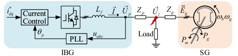
Figure 1: Low-inertia power system with PLL-based IBG. IBG is equivalent to a PLL-synchronized current source under a fault. The grid side is equivalently represented using an SG. The IBG and SG are connected to the load through line impedances $Z_{p}$ and $Z_{g}$, respectively.

Figure 2: Simplified circuit of the IBG-SG system.

II-A Swing Equation of SG

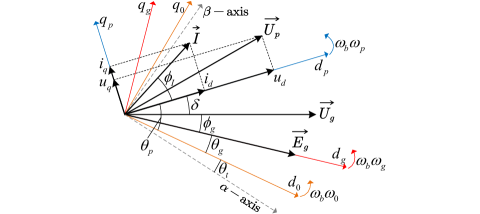
Figure 3: Voltage and current vectors with different reference frames [21]. The ${\alpha}$-, ${d_{0}}$-, ${d_{g}}$-, and ${d_{p}}$-axes represent the two-phase stationary reference frame, SRF, SG frame and PLL frame, respectively. ${\theta_{t}}=\omega_{b}\omega_{0}t$ denotes the angle between the SRF and the two-phase stationary reference frame. ${\theta_{g}}$, the angle between the ${d_{0}}$- and ${d_{g}}$-axes, represents the SG frame angle in the SRF. ${\theta_{p}}$, the angle between the ${d_{p}}$- and ${d_{0}}$-axes, represents the PLL frame angle in the SRF.

The fault-on duration is usually short, and the primary frequency control of the SG is not triggered at this stage [22]. Consequently, the dynamics of the SG are regulated using the physical inertial response. The dynamics of the SG can be expressed as a swing equation (2). The damping term of the SG is ignored because the damping effect of the SG is much weaker than that of the PLL [13, 15].

$$\begin{aligned} \frac{{d{\theta_{g}}}}{{dt}}&={\omega_{b}}\left({{\omega_{g}}-{\omega_{0}}}\right)\\ {T_{g}}\frac{{d{\omega_{g}}}}{{dt}}&={P_{m}}-{P_{g}}\end{aligned}$$ (2)

where ${T_{g}}$ denotes the inertia time constant, ${P_{m}}$ denotes the mechanical input power, and ${P_{g}}$ represents the electromagnetic output power. According to the circuit principle,

where

$${\phi_{G}} =\angle\left({{Z_{g}}+{Z_{l}}}\right)$$ (3a)

$${U_{g}}\angle{\phi_{g}} =\frac{{{Z_{l}}}}{{{Z_{g}}+{Z_{l}}}}{E_{g}}\buildrel\Delta\over{=}{{\vec{U}}_{g}}.$$ (3b)

II-B Modeling of PLL-Based IBG

Figure 4: Typical structure of the PLL. The structure is adapted so that the output of the PLL, the angle $\theta_{p}$, is referenced to the $d_{0}$-axis.

The dynamics of the terminal filter and current loop of the IBG are usually neglected in transient stability analysis [1]. Then, the IBG is deemed to be equivalent to a PLL-synchronized current source during the fault-on period. The currents ${{i_{d}}=i_{d}^{*}}$ and ${{i_{q}}=i_{q}^{*}}$ are guaranteed, where $i_{dq}^{*}=i_{d}^{*}+ji_{q}^{*}$ represents the current reference provided to the IBG. Based on the grid codes, the reactive current of IBG is required to be injected into the grid to support the voltage under a severe fault [21].

Fig. 4 shows a typical structure of the PLL. The PLL dynamics are expressed as

$$\begin{aligned} \frac{{d{\theta_{p}}}}{{dt}}&={\omega_{b}}\left({{\omega_{p}}-{\omega_{0}}}\right)\\ \frac{{d{\omega_{p}}}}{{dt}}&={K_{p}}\frac{{d{u_{q}}}}{{dt}}+{K_{i}}{u_{q}}\end{aligned}$$ (4)

where $K_{p}$ and $K_{i}$ denote the proportional and integral gains of the PI regulator, respectively. The PLL detects the PCC voltage and estimates the ${q_{p}}$-axis component ${u_{q}}$ in the PLL frame. In the SRF, the PCC voltage is obtained as

where

Lemma 1 (The first mean value theorem for the integral[29]). Let $\phi,\psi:[a,b]\to\Re$ be continuous in $[a,b]$. If the sign of $\psi$ never changes in $[a,b]$, there exists a number $c\in[a,b]$ such that

$$\begin{aligned} \int_{a}^{b}{\phi\left(x\right)\psi\left(x\right)}dx=\phi\left(c\right)\int_{a}^{b}{\psi\left(x\right)}dx.\end{aligned}$$ (23)

Based on the theorem, the two LOS types identified in Section III-A are discussed separately.

III-C1 Accelerating-Type LOS

Moving from $\delta_{e}$ to $\delta_{2}$ yields

$$\begin{aligned} &\Delta{E_{dis,2}}\\ =~{}&d\int_{{\delta_{e}}}^{{\delta_{2}}}{\left({\cos\delta\Delta\omega}\right)}d\delta\\ =~{}&d\int_{{\delta_{e}}}^{{\pi\mathord{\left/{\vphantom{\pi 2}}\right.\kern-1.2pt}2}}{\left({\cos\delta\Delta\omega}\right)}d\delta+d\int_{{\pi\mathord{\left/{\vphantom{\pi 2}}\right.\kern-1.2pt}2}}^{{\delta_{2}}}{\left({\cos\delta\Delta\omega}\right)}d\delta\\ =~{}&d\Delta{\omega_{a1}}\int_{{\delta_{e}}}^{{\pi\mathord{\left/{\vphantom{\pi 2}}\right.\kern-1.2pt}2}}{\left({\cos\delta}\right)}d\delta-d\Delta{\omega_{a2}}\int_{{\delta_{2}}}^{{\pi\mathord{\left/{\vphantom{\pi 2}}\right.\kern-1.2pt}2}}{\left({\cos\delta}\right)}d\delta\\ =~{}&d\left({1-\sin{\delta_{e}}}\right)\left({\Delta{\omega_{a1}}-\Delta{\omega_{a2}}}\right)\end{aligned}$$ (24)

where $\Delta{\omega_{a1}}$ and $\Delta{\omega_{a2}}$ represent values within the deceleration interval $\left({{\delta_{e}},~{}{\pi\mathord{\left/{\vphantom{\pi 2}}\right.\kern-1.2pt}2}}\right)$ and $\left({{\pi\mathord{\left/{\vphantom{\pi 2}}\right.\kern-1.2pt}2},~{}{\delta_{2}}}\right)$, respectively. Because ${\delta_{e}}\in\left({-{\pi\mathord{\left/{\vphantom{\pi 2}}\right.\kern-1.2pt}2},{\pi\mathord{\left/{\vphantom{\pi 2}}\right.\kern-1.2pt}2}}\right),{\delta_{2}}\in\left({{\pi\mathord{\left/{\vphantom{\pi 2}}\right.\kern-1.2pt}2},{{3\pi}\mathord{\left/{\vphantom{{3\pi}2}}\right.\kern-1.2pt}2}}\right)$, the sign of $\cos\delta$ will not change in the internal $\left({{\delta_{e}},{\pi\mathord{\left/{\vphantom{\pi 2}}\right.\kern-1.2pt}2}}\right)$ and $\left({{\pi\mathord{\left/{\vphantom{\pi 2}}\right.\kern-1.2pt}2},{\delta_{2}}}\right)$. Thus, the first mean value theorem for the integral can be used in (24). In the interval $\left({{\delta_{e}},~{}{\delta_{2}}}\right)$, the representation of $\Delta{\omega_{a2}}<\Delta{\omega_{a1}}$ is drawn for ${{d\Delta\omega}\mathord{\left/{\vphantom{{d\Delta\omega}{dt}}}\right.\kern-1.2pt}{dt}}<0$. Then, $\Delta{E_{dis,2}}>0$ is obtained from (24). In particular, if the maximum relative angle ${\delta_{max}}<\delta_{2}$, $d\int_{{\pi\mathord{\left/{\vphantom{\pi 2}}\right.\kern-1.2pt}2}}^{{\delta_{max}}}{({\cos\delta\Delta\omega)}}d\delta>d\int_{{\pi\mathord{\left/{\vphantom{\pi 2}}\right.\kern-1.2pt}2}}^{{\delta_{2}}}{({\cos\delta\Delta\omega)}}d\delta$ in (24) is obtained. Consequently, the conclusion $\Delta{E_{dis,2}}>0$ still holds. The analysis and conclusion are also applicable to the backward movement from $\delta_{2}$ to the SEP $\delta_{e}$.

III-C2 Decelerating-Type LOS

Analogous to (24), the energy dissipation of the damping term from $\delta_{e}$ to $\delta_{1}$ is derived as

$$\Delta{E_{dis,1}}=d\left({1+\sin{\delta_{e}}}\right)\left({\Delta{\omega_{d2}}-\Delta{\omega_{d1}}}\right)$$ (25)

where $\Delta{\omega_{d1}}$ and $\Delta{\omega_{d2}}$ denote values within the acceleration interval $\left({{\delta_{1}},-{\pi\mathord{\left/{\vphantom{\pi 2}}\right.\kern-1.2pt}2}}\right)$ and $\left(-{{\pi\mathord{\left/{\vphantom{\pi 2}}\right.\kern-1.2pt}2},~{}{\delta_{e}}}\right)$, respectively. In the acceleration interval $\left({{\delta_{1}},~{}{\delta_{e}}}\right)$, the representation of $\Delta{\omega_{d2}}>\Delta{\omega_{d1}}$ is drawn for ${{d\Delta\omega}\mathord{\left/{\vphantom{{d\Delta\omega}{dt}}}\right.\kern-1.2pt}{dt}}>0$. Then, $\Delta{E_{dis,1}}>0$ is obtained from (25). In particular, if the minimum relative angle is larger than $\delta_{1}$, $\Delta{E_{dis,1}}>0$ still holds. The analysis and conclusion are also applicable to the forward movement from $\delta_{1}$ to the SEP $\delta_{e}$.

In summary, $\Delta{E_{dis}}>0$ always holds for all one-direction movements from or to the SEP or their combinations, irrespective of the trajectory. In such cases, the varying cosine damping term introduces a positive energy dissipation in the system with typical parameters ($\alpha\gg 1$, $\varphi\approx 0$), benefiting the transient stability of the IBG-SG system.

IV Transient Stability Assessment

Two possible types of LOS scenarios are identified in Section III-A. When an SEP exists, the occurrence of the LOS will depend on the initial state and dynamic performance of the system [15, 11].

IV-A Unified Criterion for Two Types of New LOS Scenario

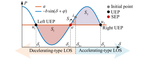
Figure 9: $P$-$\delta$ curves of the delta-power-frequency model (LABEL:eq.12). In the interval $(\delta_{1},~{}\delta_{e})$, $\Delta\omega$ increases for $a>-b\sin\left({\delta+\varphi}\right)$. $S_{1}$ represents the acceleration area. Similarly, in the interval $(\delta_{e},~{}\delta_{2})$, $\Delta\omega$ decreases for $a<-b\sin\left({\delta+\varphi}\right)$. $S_{2}$ and $S_{3}$ represent the deceleration areas.

As shown in Fig. 9, without considering the damping effect, the offset term $a$ and sine term $-b\sin\left({\delta+\varphi}\right)$ determine the movement. The motion from the initial point $i(\delta_{0}+,\Delta\omega_{0}+)$ to a point $M(\delta_{M},\Delta\omega_{M})$ ($M$ can be any point, such as point $u_{1}$ or $u_{2}$) satisfies

where ${\Delta{E_{p,M}}}$ denotes the change in potential energy from the initial point $i$ to the point $M$. The critical condition to reach the point $M$ is $E_{k,M}=0$. In other words, the critical initial kinetic energy ${E_{k,0+(cri)}}$ is equal to the change in potential energy.

If the initial kinetic energy is smaller than the critical initial kinetic energy (i.e., ${E_{k,0+}}<{\Delta{E_{p,M}}}$), the system cannot reach the point $M$.

Based on the definition of the Riemann integral, the area enclosed by the two curves $a$ and $-b\sin\left({\delta+\varphi}\right)$ in Fig. 9 is equal to the change in potential energy. Then, the change in the potential energy from the initial point $\delta_{e}$ to UEPs $u_{1}$ and $u_{2}$ is represented as $\Delta{E_{p,1}}$ and $\Delta{E_{p,2}}$, respectively.

$$\begin{aligned} \Delta{E_{p,1}}={S_{1}}-{S_{2}},\Delta{E_{p,2}}={S_{3}}.\end{aligned}$$ (26)

IV-A1 Accelerating-Type LOS

If $a>0$ and the system reaches the right UEP $u_{2}$, the accelerating-type LOS will occur. Therefore, the stability condition for the accelerating-type LOS is given by

IV-A2 Decelerating-Type LOS

If $a<0$ and the system reaches the left UEP $u_{2}$, the decelerating-type LOS will occur. Then, the stability condition for the decelerating-type LOS is reduced to

IV-A3 Unified Transient Stability Criterion

The system shows transient stability if neither the accelerating-type LOS nor the decelerating-type LOS occurs. Consequently, the stability conditions of (IV-A1) and (IV-A2) should be satisfied. Then, a unified criterion for the two LOS types is summarized: the system is transient stable during the fault-on period if (IV-A3) is satisfied.

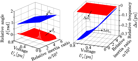
Figure 10: Curves of the initial state and SEP state variables under different relative inertia ratios and fault depths. The blue surface denotes the initial value at the moment of the fault, and the red surface denotes the SEP value.

IV-B Conservativeness Analysis on the Criterion

In the SG swing equation, a constant positive damping coefficient increases the acceleration area and reduces the deceleration area, affording conservativeness of the criterion without considering the damping term [27, 30, 28]. Alternatively, a constant negative damping coefficient affords a radical result. However, the effect of the varying damping coefficient on the transient stability is not known comprehensively in the previous studies. In the single-converter-infinite-bus system, some studies have imposed additional restrictions on the range $(\delta_{\min},~{}\delta_{\max})$ to ensure a positive damping coefficient [31, 13, 1]. In this section, we demonstrate that no additional restrictions are required to guarantee the conservativeness of the criterion under the conditions of typical system parameters.

To ensure the good dynamic performance of the PLL [1] and existence of SEP during the fault-on period, the PLL integral gain $K_{i}$ and SG inertia $T_{g}$ are adopted in a certain range: $K_{i}T_{g}$ is roughly $36$–$415$. Fig. 10 shows the curves of the initial state and SEP state variables under these typical parameters. The blue surface denotes the initial values at the moment of the fault, and the red surface denotes SEP values. This figure shows that $\delta_{0+}>\delta_{e}$ and $\Delta\omega_{0+}<\Delta\omega_{e}$ always hold under the conditions of the aforementioned system parameters. As shown in Fig. 9, starting from the initial point $i$, $\delta$ decreases ($\Delta\omega<0$) faster (${{d\Delta\omega}\mathord{\left/{\vphantom{{d\Delta\omega}{dt}}}\right.\kern-1.2pt}{dt}}<0$) to the SEP $e$. Based on the conclusion presented in Section III-C, a positive damping dissipation is achieved in the one-direction movements from or to the SEP. Consequently, the movement from the initial point to the UEP causes the energy dissipation of the system, i.e., $\Delta{E_{dis}}>0$.

A positive energy dissipation ${\Delta E_{dis}}$ yields a reduced kinetic energy ${E_{k}}$, indicating that the damping term contributes to the system stability. If the criterion shows that the typical IBG-SG system is stable, the system will operate stably. This indicates that the criterion is a sufficient condition and exhibits strict conservativeness for stability assessment under the aforementioned conditions of typical parameters.

V Simulation Verification

To adequately verify the correctness of the analysis and effectiveness of the stability criterion, simulations of the stable/unstable conditions should be conducted on the IBG-SG system in Fig. 1. Simulation experiments should be performed under the same conditions as the analytical model (LABEL:eq.12). As a result, a phasor model of Fig. 1 is developed in SIMULINK, where the IBG interface is represented by a current source [32]. Table II presents the parameters based on the literature [28, 15]. A fault occurs at $t$ = 0.5 s. The time period until 3 s is shown to exhibit the destabilization/stabilization process of the system.

TABLE II: System Parameters

Symbol	Description	Value
$S_{b}$	Base capacity	20 kVA
$U_{b}$	Base voltage	690 V
$\omega_{b}$	Base frequency	$100\pi$ rad/s
$E_{g}$	Internal electric potential of SG	1.05 pu
$P_{m}$	Mechanical power of SG	0.2465 pu
$I_{r}$	Rated current of IBG	0.8 pu
$Z_{l}$	Load impedance	0.99 + j0.1 pu
$Z_{g}$	Line impedance on the SG side	0.01 + j0.1 pu
$Z_{p}$	Line impedance on the IBG side	0.01 + j0.3 pu

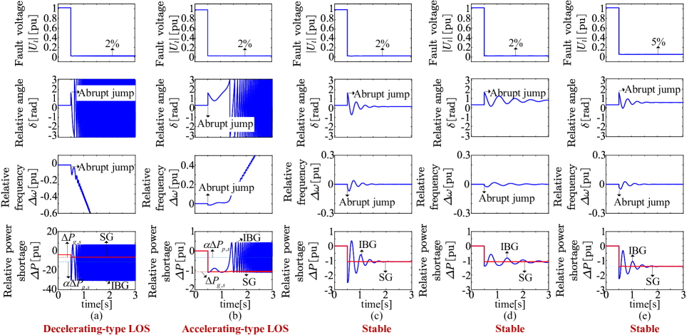
Figure 11: Simulation results of the two types of LOS. (a) Case I: decelerating-type LOS occurs when $\alpha\Delta{P_{p,s}}<\Delta P_{g,s}$. (b) Case II: accelerating-type LOS occurs when $\alpha\Delta{P_{p,s}}>\Delta P_{g,s}$. (c) Case III: system becomes stable when $K_{i}$ is adjusted to 50 ${\rm{s}}^{-1}$, and $K_{p}=0.02K_{i}$ is the same in Cases II and III to keep the damping effect of the PLL. (d) Case IV: system becomes stable when $T_{g}$ is increased to 1 ${\rm{s}}$. (e) Case V: system becomes stable when the fault is less severe, $R_{f}$ is increased to 0.12 $\Omega$, and $|U_{l}|$ is increased to 5%.

V-A Two Types of New LOS Scenarios

The jumps in $\delta$ and $\Delta\omega$ at the moment of the fault are observed in all cases in Fig. 11. The two types of new LOS scenarios are observed in Cases I and II (Fig. 11). In Case I, a large $K_{i}$ affords a large $\alpha$, inducing a smaller equivalent power shortage of the IBG than that of the SG. $\Delta\omega$ decreases, and $\delta$ oscillates. Finally, decelerating-type LOS occurs. In Case II, a small $K_{i}$ affords a small $\alpha$. The equivalent power shortage of the IBG is larger than that of the SG, thus increasing $\Delta\omega$ and oscillating $\delta$.

V-B Influence of Parameters

By adjusting the parameters considered in Case II, the system becomes stable in Cases III–V (Fig. 11 (b)–(d)). In Case II, the equivalent power shortage of the IBG is larger than that of the SG. $K_{i}$ of the PLL increases in Case III to yield an increased $\alpha$, thus changing the extreme imbalance between the equivalent power shortages of the IBG and SG. $\delta$ does not exceed left and right UEPs; thus, the system remains stable. In Case IV, $\alpha$ increases as the inertia of the SG increases, resulting in a stable system. An intuitive explanation for the stability phenomenon in Case IV is that the frequency of the SG changes at a slow pace when the inertia is large, and the IBG can keep up with the changes. Moreover, the fault becomes less severe in Case V. The redistribution of the power mitigates the equivalent power shortage of the SG and alleviates the severe mismatch between the power shortages of the IBG and SG to stabilize the system.

Table III shows that to enhance the transient stability of the system, $K_{i}$ should be adaptively selected to adjust the inertia of IBG to meet different operation conditions.

V-C Effectiveness of the Criterion

Table III shows the results of the criterion assessment and simulation. The criterion results are consistent with the simulation results. The stability/instability of the system and the LOS type are effectively evaluated. The criterion is proved to be an effective method for the transient stability assessment of the IBG-SG system.

VI Conclusion

This study analytically investigated the transient stability of low-inertia power systems with IBG. A hybrid IBG-SG system is established to characterize the transient interactions between the electromagnetic dynamics of the IBG and the electromechanical dynamics of the SG in the low-inertia grid under a fault. To describe the transient behavior of the IBG-SG system, a delta-power-frequency model is developed. Based on the model, new mechanisms from the energy perspective are revealed. First, two new LOS types, accelerating-type LOS and decelerating-type LOS, are clarified based on the relative power imbalance between the IBG and SG. In addition, a good match between the inertia of the IBG and SG balances the powers and stabilizes the system. Second, $\delta$ and $\Delta\omega$ jump abruptly at the moment of a fault, affecting the system energy. Third, the cosine damping coefficient is induced by the IBG. The damping term introduces a positive energy dissipation, beneficially affecting the transient stability. A unified criterion for the two LOS types is adopted to evaluate the system stability using the energy function method. The conservativeness of the criterion is ensured when addressing the effects of the jumps and damping term on the transient stability. The accuracy of the analysis and the effectiveness of the criterion can be verified based on the simulation results.

Regarding the transient stability issue, the findings of this study provide enlightening significance for the PLL parameters tuning, relative inertia ratio shaping, development of grid codes for fault ride-through, and future grid design. Note that the frequency regulation should be added to ensure the frequency stability of the system, which is not discussed here. Other dynamic loops, such as the DC voltage control loop, and the stability during the fault recovery period are beyond the scope of this paper, which will be analyzed in our future work.

TABLE III: Results of the Criterion and Simulation

Case	$K_{i}$	$K_{p}$	$T_{g}$	$R_{f}$	$|U_{l}|$	Condition	Criterion result	Simulation result
	[${{\rm{s}}^{-1}}$]		[$\rm{s}$]	[$\Omega$]	[$\rm{pu}$]
I	220	1	0.8	0.05	0.02	$a<0,~{}{E_{k,0+}}>{S_{1}}-{S_{2}}$	Decelerating-type LOS	Decelerating-type LOS
II	22	0.44	0.8	0.05	0.02	$a>0,~{}{E_{k,0+}}>{S_{3}}$	Accelerating-type LOS	Accelerating-type LOS
III	50	1	0.8	0.05	0.02	$a>0,~{}{E_{k,0+}}<{S_{3}}$	Stable	Stable
IV	22	0.44	1	0.05	0.02	$a>0,~{}{E_{k,0+}}<{S_{3}}$	Stable	Stable
V	22	0.44	0.8	0.12	0.05	$a>0,~{}{E_{k,0+}}<{S_{3}}$	Stable	Stable

References

- [1] X. He, H. Geng, R. Li, and B. C. Pal, “Transient stability analysis and enhancement of renewable energy conversion system during LVRT,” IEEE Trans. Sustain. Energy, vol. 11, no. 3, pp. 1612–1623, Jul. 2020.
- [2] Z. Shuai, C. Shen, X. Liu, Z. Li, and Z. J. Shen, “Transient angle stability of virtual synchronous generators using Lyapunov’s direct method,” IEEE Trans. Smart Grid, vol. 10, no. 4, pp. 4648–4661, Jul. 2019.
- [3] X. He, H. Geng, and G. Mu, “Modeling of wind turbine generators for power system stability studies: A review,” Renew. Sust. Energ. Rev., vol. 143, p. 110865, Jun. 2021.
- [4] S. Khazaee, M. Hayerikhiyavi, and S. Montaser Kouhsari, “A direct-based method for real-time transient stability assessment of power systems,” Comput. Res. Prog. Appl. Sci. and Eng. (CRPASE), vol. 6, no. 2, pp. 108–113, Jun. 2020.
- [5] Y. Xue, T. Van Cutsem, and M. Ribbens-Pavella, “A simple direct method for fast transient stability assessment of large power systems,” IEEE Trans. Power Syst., vol. 3, no. 2, pp. 400–412, May. 1988.
- [6] Y. Xue and M. Pavella, “Extended equal-area criterion: an analytical ultra-fast method for transient stability assessment and preventive control of power systems,” Int. J. Electr. Power Energy Syst., vol. 11, no. 2, pp. 131–149, Apr. 1989.
- [7] Y. Xue, T. Van Custem, and M. Ribbens-Pavella, “Extended equal area criterion justifications, generalizations, applications,” IEEE Trans. Power Syst., vol. 4, no. 1, pp. 44–52, Feb. 1989.
- [8] X. He and H. Geng, “Transient stability of power systems integrated with inverter-based generation,” IEEE Trans. Power Syst., vol. 36, no. 1, pp. 553–556, Jan. 2021.
- [9] B. Kroposki, B. Johnson, Y. Zhang, V. Gevorgian, P. Denholm, B.-M. Hodge, and B. Hannegan, “Achieving a 100% renewable grid: Operating electric power systems with extremely high levels of variable renewable energy,” IEEE Power Energy Mag., vol. 15, no. 2, pp. 61–73, Mar. 2017.
- [10] T. Ji, T. Wang, S. Huang, and M. Jin, “Comparative analysis of synchronization stability domain for power systems integrated with PMSG based on the direct method,” in Proc. 4th Inte. Conf. Energy, Electr. Power Eng. (CEEPE), Apr. 2021, pp. 547–551.
- [11] X. Wang, M. G. Taul, H. Wu, Y. Liao, F. Blaabjerg, and L. Harnefors, “Grid-synchronization stability of converter-based resources—An overview,” IEEE Open J. Ind. Appl., vol. 1, pp. 115–134, Aug. 2020.
- [12] Q. Hu, L. Fu, F. Ma, and F. Ji, “Large signal synchronizing instability of PLL-based VSC connected to weak AC grid,” IEEE Trans. Power Syst., vol. 34, no. 4, pp. 3220–3229, Jul. 2019.
- [13] X. He, H. Geng, J. Xi, and J. M. Guerrero, “Resynchronization analysis and improvement of grid-connected VSCs during grid faults,” IEEE Trans. Sustain. Energy, vol. 9, no. 1, pp. 438–450, Nov. 2019.
- [14] Q. Hu, J. Hu, H. Yuan, H. Tang, and Y. Li, “Synchronizing stability of DFIG-based wind turbines attached to weak AC grid,” in Proc. 17th Inte. Conf. Electr. Mach. Syst. (ICEMS), Oct. 2014, pp. 2618–2624.
- [15] M. G. Taul, X. Wang, P. Davari, and F. Blaabjerg, “An overview of assessment methods for synchronization stability of grid-connected converters under severe symmetrical grid faults,” IEEE Trans. Power Electron., vol. 34, no. 10, pp. 9655–9670, Oct. 2019.
- [16] H. Wu and X. Wang, “Design-oriented transient stability analysis of PLL-synchronized voltage-source converters,” IEEE Trans. Power Electron., vol. 35, no. 4, pp. 3573–3589, Apr. 2020.
- [17] X. He, S. Pan, and H. Geng, “Transient stability of hybrid power systems dominated by different types of grid-forming devices,” IEEE Trans. Energy Convers., 2021, in press.
- [18] Q. Hu, L. Fu, F. Ma, F. Ji, and Y. Zhang, “Analogized synchronous-generator model of PLL-based VSC and transient synchronizing stability of converter dominated power system,” IEEE Trans. Sustain. Energy, vol. 12, no. 2, pp. 1174–1185, Apr. 2021.
- [19] M. Zarifakis, W. T. Coffey, Y. P. Kalmykov, and S. V. Titov, “Models for the transient stability of conventional power generating stations connected to low inertia systems,” Eur. Phys. J. Plus, vol. 132, no. 6, pp. 1–13, Jun. 2017.
- [20] S. Ma, H. Geng, L. Liu, G. Yang, and B. C. Pal, “Grid-synchronization stability improvement of large scale wind farm during severe grid fault,” IEEE Trans. Power Syst., vol. 33, no. 1, pp. 216–226, Jan. 2018.
- [21] X. He, H. Geng, and S. Ma, “Transient stability analysis of grid-tied converters considering PLL’s nonlinearity,” CPSS Trans. Power Electron. Appl., vol. 4, no. 1, pp. 40–49, Mar. 2019.
- [22] F. Milano, F. Dörfler, G. Hug, D. J. Hill, and G. Verbič, “Foundations and challenges of low-inertia systems (invited paper),” in Proc. Power Syst. Comput. Conf. (PSCC), Jun. 2018, pp. 1–25.
- [23] H. Geng, L. Liu, and R. Li, “Synchronization and reactive current support of PMSG-based wind farm during severe grid fault,” IEEE Trans. Sustain. Energy, vol. 9, no. 4, pp. 1596–1604, Oct. 2018.
- [24] U. Markovic, J. Vorwerk, P. Aristidou, and G. Hug, “Stability analysis of converter control modes in low-inertia power systems,” in Proc. IEEE PES Innov. Smart Grid Technol. Conf. Eur. (ISGT-Europe), Oct. 2018, pp. 1–6.
- [25] Ö. Göksu, R. Teodorescu, C. L. Bak, F. Iov, and P. C. Kjær, “Instability of wind turbine converters during current injection to low voltage grid faults and PLL frequency based stability solution,” IEEE Trans. Power Syst., vol. 29, no. 4, pp. 1683–1691, Jul. 2014.
- [26] R. Ma, J. Li, J. Kurths, S.-j. Cheng, and M. Zhan, “Generalized swing equation and transient synchronous stability with PLL-based VSC,” IEEE Trans. Energy Convers.
- [27] Y.-H. Moon, B.-K. Choi, and T.-H. Roh, “Estimating the domain of attraction for power systems via a group of damping-reflected energy functions,” Automatica, vol. 36, no. 3, pp. 419–425, Mar. 2000.
- [28] Z. Yang, R. Ma, S. Cheng, and M. Zhan, “Problems and challenges of power-electronic-based power system stability: A case study of transient stability comparison,” Acta Physica Sinica, vol. 69, no. 8, p. 20191954, Dec. 2020.
- [29] T. M. Apostol, Calculus, Volume 1. John Wiley & Sons, 1991.
- [30] M. Y. Yousef, M. A. Mosa, A. A. Ali, S. M. E. Masry, and A. M. A. Ghany, “Frequency response enhancement of an AC micro-grid has renewable energy resources based generators using inertia controller,” Electr. Power Syst. Res., vol. 196, p. 107194, Jul. 2021.
- [31] X. Fu, J. Sun, M. Huang, Z. Tian, H. Yan, H. H.-C. Iu, P. Hu, and X. Zha, “Large-signal stability of grid-forming and grid-following controls in voltage source converter: A comparative study,” IEEE Trans. Power Electron., vol. 36, no. 7, pp. 7832–7840, Jul. 2021.
- [32] Wind energy generation systems – Part 27-1: Electrical simulation models – Generic models, IEC 61400-27-1, 2020.