Expert Aggregation for Financial Forecasting

Abstract

Machine learning algorithms dedicated to financial time series forecasting have gained a lot of interest. But choosing between several algorithms can be challenging, as their estimation accuracy may be unstable over time. Online aggregation of experts combine the forecasts of a finite set of models in a single approach without making any assumption about the models. In this paper, a Bernstein Online Aggregation (BOA) procedure is applied to the construction of long-short strategies built from individual stock return forecasts coming from different machine learning models. The online mixture of experts leads to attractive portfolio performances even in environments characterised by non-stationarity. The aggregation outperforms individual algorithms, offering a higher portfolio Sharpe Ratio, lower shortfall, with a similar turnover. Extensions to expert and aggregation specialisations are also proposed to improve the overall mixture on a family of portfolio evaluation metrics.

1 Introduction

Over the last decade, data science techniques have been regularly tested in finance to improve traditional forecasting techniques. Machine learning algorithms promise, among other things, to address the challenges of high dimensional data and to consider a broader class of functions, exploiting non-linearities or interactions in the data to improve prediction. These algorithms have been successfully applied for credit risk (Khandani et al., 2010, Butaru et al., 2016) and mortgage risk (Sadhwani et al., 2021). On the portfolio construction side, Moritz and Zimmermann (2016) use tree-based techniques to classify stock returns and build portfolios accordingly, while Heaton et al. (2017) use deep learning hierarchical models for financial prediction and classification. Additional work focuses on time series forecasting. For instance, Rapach et al. (2013) explore lead-lag relationships among country stock returns and take advantage of LASSO models to forecast stock returns in the US. Freyberger et al. (2020) use adaptive group LASSO to determine which firm characteristics provide incremental information for the cross section of expected stock returns. Hutchinson et al. (1994), Yao et al. (2000) consider a non-parametric approach with neural networks to forecast derivatives prices. Rasekhschaffe and Jones (2019), Kozak et al. (2020) explore how machine learning models can improve stock return forecasts while avoiding over-fitting. Finally, Gu et al. (2020) compare the performance of thirteen machine learning techniques including neural networks, random forests and linear models to forecast stock returns and build portfolios from the predictions.

In practice however, choosing a model and its hyper-parameters is not straightforward. Initiated by Bates and Granger (1969) and based on game theory concepts (Blackwell (1956) and Hannan (1957)), the idea of combining predictions can be very effective for predictive learning tasks. Averaging models may lead to a reduction in variance and induces smaller generalisation errors (Breiman, 2001). A key point is the diversity of the models considered in the ensemble (Brown et al., 2005a, b). Bagging (Breiman, 1996) and Boosting (Freund et al., 1996, Schapire, 1990) are for example two popular methods for generating ensembles. Combining different models has also been used to improve time series forecasts, such as exponential smoothing with ARIMA (Bai et al., 2010), AdaBoost with recurrent neural networks (Sun et al., 2018) or to forecast stock market trading patterns (Lin et al., 2021). Weng et al. (2018) predict stock prices from a neural network ensemble, a support vector ensemble, a boosted tree and a random forest. Yang et al. (2020) integrate different reinforcement learning algorithms to learn a stock trading strategy. Nti et al. (2020), Albuquerque et al. (2022) provide a comprehensive review of ensemble techniques used in finance. Nevertheless, an algorithm may outperform others during specific time periods only and such ensemble methods are not robust to data distribution changes.

To tackle unstable accuracy over time, Littlestone and Warmuth (1994) and Vovk (1990) independently introduced one successful approach for time series forecasting: the online aggregation of experts. This method allows to combine in a single approach the forecasts of a set of models, called experts (Cesa-Bianchi and Lugosi, 2006). A new forecast is obtained with the help of sequential decision techniques and is guaranteed by the theory to be on average almost as accurate as the forecast of the best expert (Freund et al., 1997, Vovk, 1997, 1998). The resulting mixture is continuously updated as soon as the expert forecasts become available. This is a desirable feature in non-stationary environments as it allows to reconsider regularly the best models. This approach is all the more appealing that it makes no assumption about the data generation process. The framework is also a way to meet the challenge of tuning hyper-parameters, by considering every possible parameter combinations with the same algorithm. In addition, aggregation with expert advice reduces the average excess risk of the estimator while benefiting from theoretically sound results on the optimal regret bound, i.e. aggregation guarantees to recover online the best possible combination of experts.

These attractive properties partly explain why sequential aggregation procedures have been intensively studied in recent years (Azoury and Warmuth, 2001, Vovk, 2006, Atiya, 2020, Petropoulos et al., 2022). The book Cesa-Bianchi and Lugosi (2006) provides an in-depth introduction to this approach. Aggregation methods have been used successfully for time series forecasting applications, such as energy consumption or electricity prices (Gaillard and Goude, 2014, Nowotarski and Weron, 2018), weather (Taillardat et al., 2016, Thorey et al., 2017), pollution (Debry and Mallet, 2014, Auder et al., 2016) or exchange rates Amat et al. (2018).

In this paper, online expert aggregation is used to address the difficulty of having to choose between several investment strategies, and to ensure robustness to changing market conditions (i.e. guarantee satisfactory performance over time). Thirteen different portfolios are constructed based on various machine learning algorithms (linear, tree-based, neural networks) forecasting one-month-ahead stock returns from firms’ financial characteristics. The dataset includes 94 characteristics (size, momentum, etc.) for a large collection of 30,000 stocks over the 1957-2016 period. Zero-net-investment portfolios are constituted based on model’s forecasts, buying stocks in the the highest expected return decile and selling stocks in the lowest. Eventually, the state-of-the-art Bernstein Online Aggregation from Wintenberger (2017) provides a convex combination of the long and short strategies based on individual experts’ forecasts to build a robust portfolio. The aggregation assigns every month a weight to each expert according to its current performance.

Results of this paper show that robust online aggregation leads to attractive portfolio performances even in adversarial environments characterised by strong non-stationarity of the data distribution. The aggregated portfolio not only outperforms the experts, but also makes the approach more robust by dynamically adapting to market changes online, which greatly reduces the shortfall risk. The aggregation allows to build an investment strategy with an annual Sharpe Ratio of 2.82, slightly higher than the best expert (a neural network) with 2.74, while having a maximum monthly loss of 7%, more than twice as low as that same best expert (16%). Eventually, the aggregated portfolio turnover stays close to the one of each individual strategy around 120%.

To our knowledge, this paper provides the first application of online expert aggregation for financial strategies. This work adds on the growing literature testing machine learning techniques for portfolio management, using an adaptive mixture of long-short portfolios based on data-driven individual stock price predictions. The contribution is plural. First, state-of-the-art Bernstein Online Aggregation (BOA) is applied on portfolio construction. The aggregation ponders directly the stock weights of each individual expert portfolio, allowing to consider any algorithm, even black-box models. Second, the tests provide a comparison of the performance of the aggregated strategy with thirteen machine learning experts, studied by Gu et al. (2020), on a large dataset (more than 30,000 US stocks). Eleven of the thirteen experts used in the paper are ensemble-based by construction for stability purposes, but also to compare the performance of online aggregation with static ensemble methods. Finally, expert and aggregation specialisations are proposed to improve the global mixture. An expert outperforming the aggregation gives the opportunity to increase the initial set of experts with additional models derived from this best expert. In the same spirit, aggregation specialisation is introduced and explores the possibility to refine the aggregation depending on the context.

2 Data and Methodology

Instead of relying only on one model forecast, a more robust approach considers ensemble forecasts. The aggregation framework considered in this paper tackles unstable accuracy of forecasting models in non-stationary environments in an online manner, without hypothesis on models and the data distribution.

2.1 Expert Aggregation

A set of forecasting algorithms, called experts, estimate independently the next value of a given sequence. A set of observations $\mathcal{D}_{t}=\{(x_{1},y_{1}),...,(x_{t},y_{t})\}$ is given at each time $t>0$ where the target $y_{t}$ is a bounded value on $\mathbb{R}$ and $x_{t}\in\mathbb{R}^{d}$ is a feature vector Each forecasting algorithm $k$ at $t$ is a function $f^{k}_{t}:\mathbb{R}^{d}\mapsto\mathbb{R}$ providing a forecast $f^{k}_{t}(x_{t+1})$ that has to be as close as possible to $y_{t+1}$. The forecasts are obtained element by element by learning the (assumed) relationship between the input space $\mathbb{R}^{d}$ and a bounded subset of $\mathbb{R}$. An online expert $f^{k}=(f^{k}_{0},f^{k}_{1},f^{k}_{2},\ldots)$ is a sequential algorithm that produces at each time $t$ an expert $f^{k}_{t}$.

The relevance of the expert’s forecast is measured at each time step by a convex loss function $\ell:\mathbb{R}\times\mathbb{R}\mapsto\mathbb{R}_{+}$. In an online setting, the goal of the experts is to minimise their cumulative empirical error $\sum_{t\geq 0}\ell(y_{t+1},f^{k}_{t}(x_{t+1}))$ between the true value $y_{t+1}$ and the expert’s forecast $f^{k}_{t}(x_{t+1})$.

Experts aggregation is a sequential forecasting framework allowing to mix several forecasting models in a robust approach (Cesa-Bianchi and Lugosi, 2006). The algorithm provides as forecast a convex combination of the outcomes from a finite set of experts, where the weights are computed according to a chosen deterministic policy. Let $f^{1},...,f^{K}$ be $K$ online experts providing bounded estimations (so that losses are bounded as well). Aggregation aims at finding the optimal online convex combination

$$f_{w}=\sum_{k=1}^{K}w_{k}f^{k}=\left(\sum_{k=1}^{K}w_{k,t}f^{k}_{t}\right)_{t\geq 0}$$

with weights $w_{k,t}\in S$ where $S$ is a closed and bounded subset of $\mathbb{R}^{K}$. In the following $S=\{w_{k}\in\mathbb{R}^{K}_{+},\sum_{k=1}^{K}w_{k}=1\}$. The performance of the online aggregation procedure is measured by the cumulative error $\sum_{t\geq 0}\ell(y_{t+1},f_{w,t}(x_{t+1}))$ between the target $y_{t+1}$ to be predicted and the mixture’s forecast $f_{w,t}(x_{t+1})$.

However, if the experts’ accuracy is low, so will be the accuracy of the mix, it is thus impossible to ensure a low cumulative loss for the aggregation in absolute terms. Therefore, the aggregation framework seeks to ensure a low cumulative error compared to the cumulative errors of the experts. To do so, the mixture is compared to the best possible fixed combination of experts, called oracle. The goal of the aggregation is thus to retrieve online the oracle.

The regret (Freund et al., 1997) compares a given online aggregation procedure with the oracle in terms of cumulative errors. The regret is defined at time $T$ by

$$R_{T}=\sum_{t=0}^{T}\ell(y_{t+1},f_{w,t}(x_{t+1}))-\inf_{u\in S}\left\{\sum_{t=0}^{T}\ell(y_{t+1},f_{u,t}(x_{t+1}))\right\},$$

where the first term is the cumulative error of the mixture and the second term is the approximation error, i.e. the cumulative error of the oracle compared to the target $y_{t+1}$ . By minimising regret, one seeks to avoid sub-optimal mixtures and thus reduce the number of actions taken where, in hindsight, a better choice would have been possible. These choices are directed by a given policy, called rule.

The rule of an aggregation determines how the weights are assigned to each expert. The rules are deterministic, need all expert forecasts at each time and depend on a learning rate parameter $\eta>0$. The learning rate, which is preferably tuned online, guides the aggregation rule adaptability to the environment. Having a high $\eta$ leads to follow the best expert, while a lower rate leads the mixture to a more uniform and conservative distribution. Many rules exist in the literature and differ according to the application. Littlestone and Warmuth (1994) and Vovk (1990) propose to use an online convex aggregation rule called Exponentially Weighted Average (EWA) allowing rough changes in the weights allocation. Multiple Learning rate (ML Poly, Cesa-Bianchi and Lugosi (2003), Gaillard et al. (2014)) has its own learning parameter calibration rule which is faster than the empirical tuning described by Devaine et al. (2013). Fixed Share forecaster (FS, Herbster and Warmuth (1998)) competes not only with the best fixed expert but also with the best sequence of experts and Ridge allows non-positive weights and non-convex combinations (Azoury and Warmuth, 2001, Vovk, 2006). Most of the aggregation rules, in particular the one used in this paper, ensure that the regret converges to zero when $T$ goes to infinity. So, this study focuses on reducing the approximation error by increasing the heterogeneity of the expert set (see Gaillard and Goude (2014) and Stoltz (2005) for further details).

This paper considers the Bernstein Online Aggregation (BOA, Wintenberger (2017)). At time $t$, BOA assigns a new weight to each expert according to its accuracy compared to the other experts, by minimising the loss $\ell_{k,t+1}=\ell(y_{t+1},f_{k,t}(x_{t+1}))-\ell(y_{t+1},f_{w,t}(x_{t+1}))$. Given the losses $\ell_{t}=(\ell_{1,t},\dots,\ell_{K,t})$ suffered by the experts at each instance $t$, BOA assigns to expert $k$ the weight

$$w_{k,t}=\frac{\exp(-\eta\ell_{k,t}(1+\eta\ell_{k,t}))}{\exp(-\eta\ell_{w,t}(1+\eta\ell_{w,t}))}w_{k,t-1},$$

where $\ell_{w,t}=\sum_{k=1}^{K}w_{k,t-1}\ell_{k,t}$ is the loss suffered at time $t$ by the aggregation at time $t-1$ (with weights $w_{t-1}$). The second order refinement of the loss is designed to penalise large errors and stabilises the weight allocation. BOA benefits from a faster rate of convergence than other rules. The learning rate $\eta$ is optimally tuned in the BOA process and ensures minimising regret with the fast rate of convergence $\log(K)/T$ in deviation. BOA procedure is reported in Algorithm 1. For further details, see Wintenberger (2017).

Algorithm 1 Bernstein Online Aggregation (BOA)

0:  weights $w_{k,0}>0$ s.t. $\sum^{K}_{k=1}w_{k,0}=1$, learning rate $\eta>0$

  for each $t=1,...,T$ do

     for each $k=1,...,K$ do

        

$$w_{k,t}=\frac{\exp(-\eta\ell_{k,t}(1+\eta\ell_{k,t}))}{\exp(-\eta\ell_{w,t}(1+\eta\ell_{w,t}))}w_{k,t-1}$$

     end for

  end for

2.2 Application to Financial Portfolio

The online aggregation procedure is applied to portfolio returns, by minimising the cumulative loss between each expert’s portfolio and the best possible portfolio, the target. The target for the long (resp. short) portfolio is obtained by buying at each rebalancing date the 10% best (resp. worst) performing stocks. In practice, the aggregation assigns at the end of each month a vector of weights to the expert portfolios to minimise the difference between the mixture returns and this optimal portfolio returns. Note that the target should not be confused with the oracle discussed in Section 2.1, which corresponds to the best possible mixture of experts (and could be very different from the target depending on the quality of the experts). Two aggregations are applied, one for the long strategies and another one for the short strategies. The best long experts are not necessarily the same as the short ones at each instant. Using two distinct aggregations allows to take advantage of different experts at different times. The returns of the long-short aggregation are the difference between the long aggregation portfolio and the returns of the short one.

2.3 Data

Data comes from Wharton Research Data Services (WRDS ), including CRSP and Compustat database, and covers more than 30,000 US stocks over 1957-2017 period. The 94 standard firm characteristics used by Gu et al. (2020) are considered as features to feed the stock return forecasting algorithms. Twenty among these features are updated monthly, thirteen updated quarterly and sixty-one updated annually. Following Gu et al. (2020) and Freyberger et al. (2020), a cross-section rank transformation is performed each month on all firm characteristics that maps these ranks into the $[-1,1]$ interval. Missing data are replaced by their cross-sectional median. In order to avoid forward-looking bias (information at month $t$ is only known at month $t+1$ for monthly characteristics, $t+4$ for quarterly and $t+6$ for annual ones), monthly variables are delayed by one month, quarterly data by four months, and annual data by six months.

3 Expert Portfolio

The online aggregation is compared to the strategies based on single forecasting algorithms and follow the same methodology as Gu et al. (2020) regarding data construction, forecasting windows and models construction. This section describes the datasets and the thirteen forecasting models. Then, the performance of long-short strategies based on individual experts is presented.

3.1 Forecasting Models

Stocks are characterised by a set of features, such as firm size or stock return momentum. For each month and each stock, a forecasting model is fed with these features to predict next month return. Due to computationally intensive forecasting procedures, the models are re-calibrated only each year. The training set size starts in 1957 with 18 years and increases with time. Models are re-fitted by increasing the training sample by one year. The validation set size of 12 years is maintained constant by rolling it forward to include the most recent year. The unobserved one-year testing set is picked within a 30-year period from 1987 to 2016. So, the first training (over 30 ones) is done on the 1957-1974 period, the validation on 1975-1986 and the out-of-sample test on year 1987. The second training is then done on 1957-1975, validation on 1976-1987, test on 1988, and so on until the testing year reaches 2016.

A unique model per method is trained for all stocks, and the model stays the same over the training period as done in Gu et al. (2020). This avoids intensive computational costs and tends to stabilise return estimates of individual stocks. Note that the forecasting models are not strictly online, but their associated portfolios are, consistent with the online aggregation framework. The thirteen models are reported in Table 1 and their hyper-parameters in Table A.6 in Appendix.

Family	Model
Linear	Ordinary Least Square (OLS+H)
	Ordinary Least Square 3 factors (OLS3+H)
	Generalised Linear Model with group Lasso (GLM+H)
	Elastic Net (ENet+H)
Linear with	Partial Least Square (PLS)
dimension reduction	Principal Component Regressor (PCR)
Tree-based	Random Forest (RF)
	Gradient Boosting Regressor Tree (GBRT+H)
Neural network	Neural Networks (NN1-NN5)

Table 1: Forecasting Model Description.

Models are trained by minimising the squared error between the observed and the estimated stock returns, except for models followed by “+H” indicating the use of Huber loss defined in Appendix B. Huber loss minimises the squared loss when residuals are below an (optimised) threshold and the absolute loss above. Huber is thus robust to outliers while not ignoring their effects.

Except for Partial Least Square (PLS) and Principal Component Regressor (PCR), all the models are ensemble-based by construction. A given model is trained several times on the dataset, then averaged to produce the forecast. This allows to stabilise the estimators, reducing over-fitting for the linear models with Huber loss and the neural networks trained using gradient descent, but also to compare aggregation with static ensemble methods.

The performances of the forecasting models are reported in Table C.8 in Appendix. Following Lewellen (2014), the accuracy of three basic forecasting benchmarks is shown in Table A.7 in Appendix, based on three ordinary least squared regressions with respectively 3, 7 or 15 variables.

3.2 Performance of Experts’ Portfolios

Stocks are sorted according to each model’s predictions. A long (resp. short) portfolio is built by buying 10% of the stocks having the highest (resp. lowest) estimated returns. Both equally and value weighted portfolios are considered. Value weighted results are presented in the appendix. Value weighted portfolios are less sensitive to illiquidity of small cap stocks, but as the objective functions of both forecasting models and aggregation minimize equally weighted forecast errors, the main paper focuses on equally weighted portfolios. When comparing portfolio performance with the estimation accuracy in Table C.8, improved forecasts do not necessarily lead to better portfolios. For instance, the portfolio OLS+H outperforms the experts based on linear and tree algorithms, while having one of the lowest %R2 among the forecasting models. Average monthly returns generally increase monotonically decile by decile for each algorithm, as reported in Appendix Table C.9 for equally weighted portfolios and Table C.10 for value weighted.

Table 2 reports the performances of each expert portfolio on the out-of-sample test period. The performance metrics definitions are precised in Appendix B. In general, expert performance improves with the model complexity. An exception occurs with the linear model OLS+H which provides similar performance to the neural networks. Portfolio performances are in line with forecast accuracy results. Neural network offer the best portfolio performance, outperforming the other strategies with an annual Sharpe Ratio (SR) always greater than 2.2. The expert NN2 dominates the other algorithms with an annual return of 0.5 for the equally weighted portfolio and 0.37 for value weighted, leading to a SR of 2.74 and 2.67 respectively. Linear models ENet+H and GLM+H are also valuable strategies, with a SR of 1.77 and 1.81 respectively, very close to experts based on dimension reduction (PLS 1.85 and PCR 1.78). Tree-based models GBRT+H and RF have a SR of 1.71 and 1.96 respectively, thanks to their low volatility (0.15 and 0.14 respectively). Surprisingly, OLS+H proposes a comparable SR (2.28) as neural networks. While the model is restricted to linear functions and not particularly well fitted for high-dimensional data, when considering long-short stock strategies, OLS+H competes with more sophisticated models able to deal with non-linear relationships between variables. OLS3+H (which has a limited number of stock characteristics) has the lowest SR at 1.1.

	OLS	OLS3	PLS	PCR	ENet	GLM	RF	GBRT	NN1	NN2	NN3	NN4	NN5
	+H	+H			+H	+H		+H
Ann Ret	0.36	0.21	0.31	0.30	0.30	0.32	0.28	0.25	0.48	0.50	0.48	0.48	0.43
Vol	0.16	0.19	0.17	0.17	0.17	0.18	0.14	0.15	0.20	0.18	0.20	0.19	0.20
SR	2.28	1.11	1.85	1.78	1.77	1.81	1.96	1.71	2.39	2.74	2.42	2.56	2.21
Skew	0.52	0.77	0.14	0.46	-0.05	-0.26	0.97	1.72	2.18	2.27	1.69	1.75	2.40
Kurt	4.36	17.89	7.96	7.50	7.42	8.63	7.03	12.63	19.44	13.94	11.12	11.47	19.56
Max DD	0.25	0.63	0.44	0.31	0.40	0.40	0.23	0.24	0.28	0.17	0.29	0.23	0.47
Max Loss	0.13	0.36	0.23	0.20	0.22	0.27	0.17	0.16	0.28	0.16	0.23	0.22	0.23
Turnover	1.26	1.50	1.15	1.27	1.28	1.36	0.92	1.25	1.24	1.23	1.20	1.20	1.15

Table 2: Performance of Experts’ Portfolios

Note: This table presents the performance of long-short strategies based on individual forecasting models. Columns Ann Ret, Vol, Skew, Kurt, SR, Max DD, Max Loss and Turnover stand for annualised average return, volatility, skewness, kurtosis, annual Sharpe Ratio, maximum drawdown, 1-month maximum loss and portfolio turnover. The metrics are computed on the test period 1987-2016. Portfolios are equally weighted.

At first sight, selecting a best strategy is not obvious. NN2 offers better returns and SR, but the low turnover of RF (92% against an average of 120%) or the low maximum monthly loss of OLS+H (13%) makes these strategies appealing in practice. NN5, although appealing in terms of SR, is characterised by higher extreme risks (highest kurtosis among all experts and a maximum drawdown substantially greater than that of NN2 (47% against 17%). The qualitative conclusions remain when considering value weighted portfolios (reported in Table C.11 in Appendix).

4 Aggregation of Portfolios

This section shows how the aggregation of individual strategies based on machine learning models can enhance portfolio performance and adapt to changing market conditions. Variant aggregations that improve the mixtures in specific contexts are presented. Finally, the importance of each expert in the aggregation is examined and expert specialisation is discussed.

4.1 Aggregated Portfolio Performance

	Best Expert	Fixed Combination		Adaptative Mixture		Oracle
	NN2	PtfUNI	Best Convex	Best Convex	PtfBOA	Best Convex
			on Valid. Set	One-year Rolling
Ann Ret	0.50	0.36	0.36	0.43	0.49	0.50
Vol	0.18	0.14	0.16	0.16	0.18	0.17
SR	2.74	2.56	2.28	2.60	2.77	2.92
Skew	2.27	1.19	0.52	1.65	3.11	2.90
Kurt	13.94	10.17	4.36	10.58	19.63	17.93
Max DD	0.17	0.24	0.25	0.17	0.08	0.07
Max Loss	0.16	0.18	0.13	0.16	0.08	0.07
Turnover	1.23	1.22	1.26	1.22	1.23	1.24

Table 3: Performance of Aggregated Portfolios.

Note: Columns Ann Ret, Vol, Skew, Kurt, SR, Max DD, Max Loss and Turnover stand for annualised average return, volatility, skewness, kurtosis, annual Sharpe Ratio, maximum drawdown, 1-month maximum loss and portfolio turnover. The metrics are computed on the test period 1987-2016. Expect for NN2, all the portfolios are convex combinations of the thirteen experts. The best convex combination on the validation set is a fixed combination calibrated on 1986. The best convex one-year rolling mixture assigns the best convex combination of experts estimated the previous year to the next year. The oracle is the best possible convex mixture on the test period, unachievable in practice. Portfolios are equally weighted.

BOA rule is applied on the expert portfolios, minimising the square loss between the best possible portfolio returns and the returns of the $K=13$ expert strategies listed in Table 1. The resulting portfolio is called PtfBOA. By dynamically weighting strategies, one can expect to retrieve (at least) the best expert’s portfolio returns and reduce the risk of betting on only one expert. A uniform mixture of the $K$ portfolios, called PtfUNI, is used as a benchmark and assigns a constant weight of $1/K$ to each expert throughout the test period.

Table 3 shows the best expert in terms of annual Sharpe Ratio (NN2), PtfUNI, PtfBOA and the oracle, i.e. the best possible convex combination over the test period, unachievable in practice. Two additional mixtures are presented to compare BOA with simple ensemble approaches. The best convex combination calibrated over the last year of the validation set provides a fixed weighting that is less naive than the uniform mixture. To adapt to changing market conditions, the best one-year rolling convex mixture assigns the best fixed convex combination estimated the previous year to the next year. The latter does not benefit from the same theoretical guarantees than BOA and can induce rough variations in portfolio weights through time.

The aggregation PtfBOA brings a significant improvement to classical machine learning techniques and the different mixtures. BOA portfolio provides the highest SR at 2.77, followed by NN2 (2.74), while decreasing substantially the portfolio maximum monthly loss (8%) compared to NN2 and all portfolios. PtfBOA has the highest skewness (3.11) and the lowest max DD (8%), with a similar turnover (123%) as NN2 and the mixtures. These results are all the more encouraging that the expert aggregation does not directly optimise these indicators, but only considers the error between the monthly returns of the expert portfolios and the target. The uniform aggregation PtfUNI offers the third best SR at 2.56, ex-aequo with NN4, despite lower annalised returns (0.36) compared to NN2 and PtfBOA. Value weighted strategies give similar results (see Table C.12 in Appendix), PtfBOA being able to outperform the experts and mixtures in multiple metrics. As expected, the turnover of all value weighted portfolios is lower than in the equally weighted case.

The oracle’s SR (2.92) indicates that there is only marginal room for improvement, by designing better objective functions or better rules for the online aggregation. The two simple ensemble-based portfolios (the fixed and one-year rolling best convex combination), with a SR of 2.28 and 2.60 respectively, do not manage to beat the best expert. Both mixtures also underperform PtfBOA in terms of returns, SR, max DD and max Loss. To put emphasis on the relationship between experts and the online aggregation, the following analysis focuses on PtfBOA and PtfUNI.

4.2 Mixture Analysis

Weights analysis

Figure 1 displays the dynamic weights of the thirteen experts within BOA as well as the cumulative log returns of both long and short strategies. The bottom graph highlights how aggregation proceeds: starting with uniform weights, a transition phase over the first few months gives way to the best experts until the mixture converges.

The mixture favors neural networks and OLS+H. NN2 is the best expert all over the test period for the long strategy in terms of cumulative returns. The linear model OLS+H is the best expert for the short strategy before 2001, and therefore share a large part of the weighting in the mixture (aroung 40%). In 2001, a regime break (coinciding with the dot.com bubble burst) reduces OLS+H importance in the mixture at the benefit of neural networks. Aggregation adapts quickly its weights during the 2001 regime shifts, which partly explains the attractive performance and robustness of the strategy. PtfBOA is the second best profitable strategy, for both the long and short portfolios. It is worth noting that the difference in cumulative performance between PtfBOA and PtfUNI is large, and encourages the adoption of an online mixture.

Over the entire test period, expert weights are relatively stable from 1992 to 2000 and then from 2001 until 2016. These two regimes of stable outperformance of the best experts encourage the mix to “follow the leader” instead of considering a more heterogeneous mixture. This is an interesting result, especially in a non-stationary environment where the most profitable strategy may vary from one instant to the next. Here, aggregation is based mainly on the best portfolio and benefits little from the opinion of the other experts.

Interestingly, during the 2008 Subprime crisis, all experts and the aggregation experience a large drop in performances. However, the crisis has only a small impact on individual experts’ weights in the aggregation. Neural networks manage to get higher average returns compared to the other experts on this specific period, and thus retain their dominant position in the mix (Figure C.7 in Appendix).

Average weights of the experts on the test period are given in the Table C.13 in Appendix. In particular, NN2 and OLS+H share 67% of the weight allocated to the thirteen strategies on average over the test period. PtfBOA has the closest weight combination to the oracle.

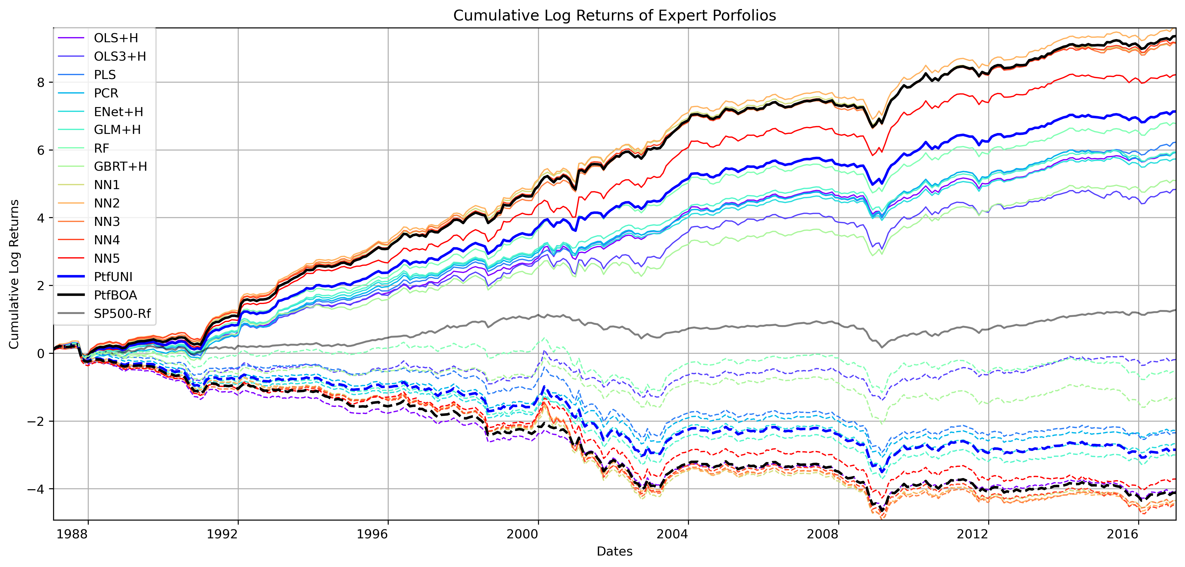
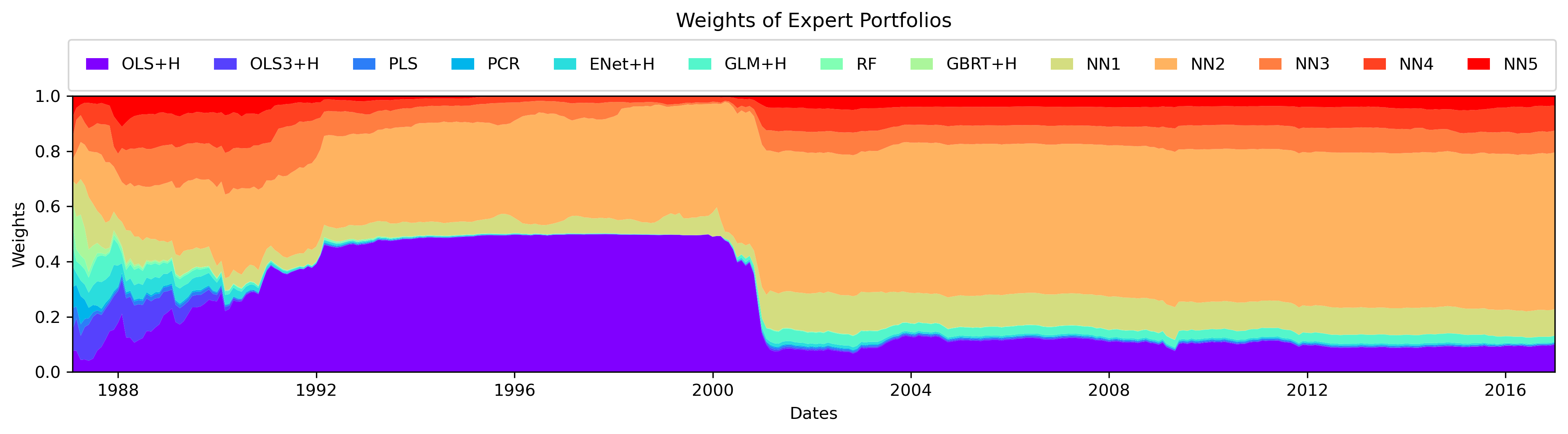
Figure 1: Cumulative Returns of Portfolios and Experts’ Weights of PftBOA.

Note: The first graph presents cumulative log returns of portfolios on the test period as well as S&P500 (in gray). Full lines (resp. dash lines) indicate long positions (resp. short). Black bold lines correspond to aggregation PtfBOA and blue bold lines to the uniform mixture PtfUNI. Both aggregations include the 13 strategies OLS+H, OLS3+H, PLS, PCR, ENet+H, GLM+H, RF, GBRT+H, NN1, NN2, NN3, NN4, and NN5. The bottom graph plots the average expert weights of the long and short aggregations of PtfBOA over the period. Portfolios are equally weighted.

Experts ranking

Figure 2 illustrates the distribution of each Sharpe Ratio’s rank for the thirteen individual experts, the uniform mixture and the two aggregations (PtfBOA and PtfUNI). Each column indicates the number of time that the strategy has been ranked 1, 2, 3, $\dots$, 15 in terms of SR over the test period (1987-2016). PtfBOA reaches rank 1 close to 17% of the time over the test period, followed by OLS+H (13%). However, OLS+H is often one of the least profitable experts, as illustrated by its significant proportion among low ranks (from 9 to 15). The five neural networks (over thirteen experts) and PtfBOA represent more than half of the overall area on the top 3 ranks. In particular, PtfBOA appears in 14% of the top 3 SR, when OLS+H reaches 11% and NN2 9%, close to the uniform mixture PtfUNI 8%. Besides, the ranks of NN2 or OLS+H are more disparate compared to the ranks of the aggregation.

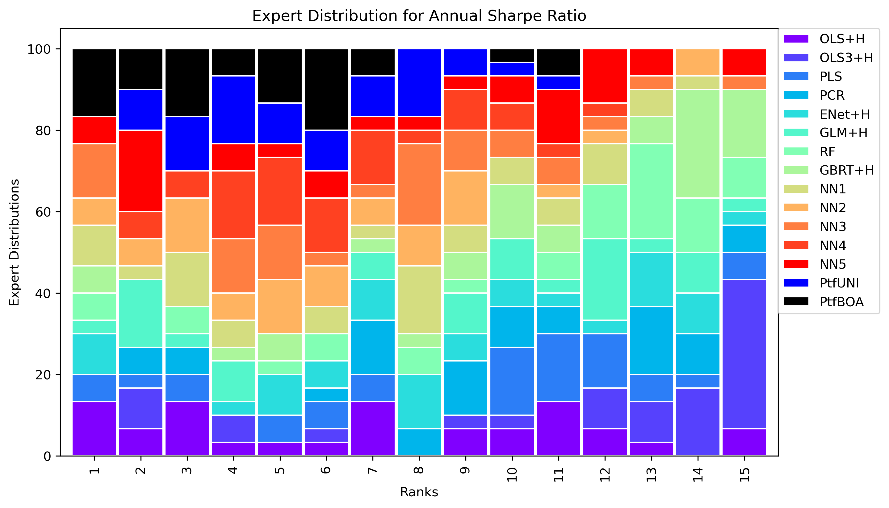
Figure 2: Experts’ Sharpe Ratio Ranks Distribution.

Note: This graph presents the distribution of each annual Sharpe Ratio’s rank for the thirteen individual experts, the uniform mixture and the two aggregations (PtfBOA and PtfUNI). The distribution is obtained by counting the number of times an expert gets the best, second (and so on) Sharpe Ratio. Portfolios are equally weighted.

4.3 Sub-samples Analysis

In this section, the aggregation is performed on two sub-samples of US stocks, specifically the top and bottom 1000 stocks in terms of market capitalisation. The aim is to test if the aggregation performance hold on the sub-sample of large stocks, because small and micro cap stocks may be more difficult to trade frequently due to liquidity issues.

	OLS	OLS3	PLS	PCR	ENet	GLM	RF	GBRT	NN1	NN2	NN3	NN4	NN5	PtfUNI	PtfBOA
	+H	+H			+H	+H		+H
	Top 1000 Market Caps
Ann Ret	0.15	0.06	0.13	0.13	0.06	0.06	0.08	0.05	0.16	0.17	0.15	0.15	0.11	0.11	0.13
Vol	0.16	0.18	0.17	0.16	0.18	0.18	0.16	0.14	0.23	0.22	0.24	0.23	0.21	0.14	0.14
SR	0.94	0.34	0.79	0.78	0.34	0.34	0.52	0.39	0.70	0.76	0.64	0.65	0.54	0.82	0.95
	Bottom 1000 Market Caps
Ann Ret	0.48	0.58	0.46	0.47	0.58	0.58	0.83	0.73	0.97	1.01	0.97	0.96	0.87	0.73	0.97
Vol	0.21	0.26	0.23	0.23	0.26	0.26	0.34	0.32	0.38	0.40	0.39	0.38	0.42	0.24	0.37
SR	2.25	2.21	1.99	1.99	2.21	2.21	2.43	2.26	2.57	2.56	2.51	2.5	2.09	3.07	2.59

Table 4: Statistical Performance of Sub-portfolios: Small and Large Caps.

Note: This table presents the performance of individual experts portfolios, PtfUNI and PtfBOA on two different sub-samples: the top 1000 and the bottom 1000 stocks in terms of market capitalisation. Columns Ann Ret, Vol, SR report annualised average return, volatility and annual Sharpe Ratio. The metrics are computed on the test period 1987-2016. Portfolios are equally weighed.

Table 4 reports the Sharpe Ratios of experts and aggregation-based strategies on the two different market capitalisation universes. It is striking to see that the best experts are very different on the two universes of stocks. OLS+H provides the highest SR (0.94) among the largest stocks (top 1000), while NN1 is the best expert on small stocks (bottom 1000) with a SR at 2.57, very close to NN2 at 2.56. However, PtfBOA outperforms all individual experts for the universe of large stocks, with a SR of 0.95, and an attractive SR (2.59) on the smallest ones. The naive constant weighting PtfUNI provides the highest SR for small stocks (3.07). Depending on the stock size, best experts differ and the online aggregation allows to adjust experts’ weights accordingly.

4.4 Improving Aggregation

A strong advantage of the aggregation lies also in its easy adaptation to alternative objectives. Two improvements of the aggregation are proposed, either by adding some prior in the global mixture (Section 4.4.1) or by specialising the best experts (Section 4.4.2).

4.4.1 Pre-trained Aggregation

At initialisation, expert’s weights are uniformly set (at 1/K with $K$=13 the number of experts) and are then updated according to their losses and BOA rule. In order to speed up the convergence, one can pre-train the online mixture on the last year of the validation set, namely 1986. Thus, over the year 1987, the aggregation benefits from a prior.

	Best Expert (NN2)	PtfUNI	Original BOA	Pre-trained BOA
Ann Ret	0.50	0.36	0.49	0.49
Vol	0.18	0.14	0.18	0.17
SR	2.74	2.56	2.77	2.78
Skew	2.27	1.22	3.11	3.15
Kurt	13.94	10.49	19.63	19.66
Max DD	0.17	0.24	0.08	0.08
Max Loss	0.16	0.18	0.08	0.08
Turnover	1.23	1.22	1.23	1.23

Table 5: Pre-trained Aggregation Portfolio Performance.

Note: Columns Ann Ret, Vol, SR, Skew, Kurt, Max DD, Max Loss and Turnover stand for annualised average return, annualised volatility, annual Sharpe Ratio, skewness, kurtosis, maximum drawdown, 1-month maximum loss and portfolio turnover. Metrics are computed on the test period. Portfolios are equally weighted.

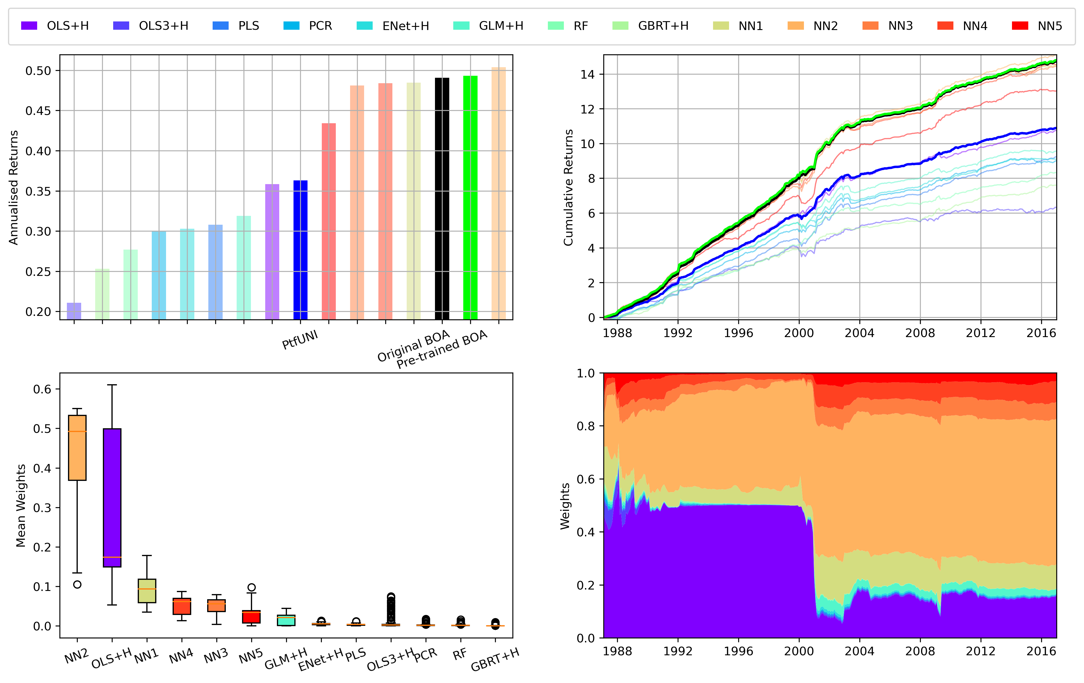
Figure 3: Pre-trained Aggregation Analysis.

Note: These four graphs present on the first row: average returns (left) and cumulative log returns (right) of the experts, the original PtfBOA, the pre-trained PtfBOA and PtfUNI ; on the second row: average weights of the pre-trained PtfBOA (left) and their evolution on the test period (right). PtfBOA is pre-trained during the year 1986 and then tested on 1987-2016 period.Portfolio are equally weighted.

Figure 3 presents the portfolio returns and corresponding weights of the pre-trained BOA. The top left and top right graphs display respectively the average monthly returns and the cumulative log returns of all the strategies. Like the original PtfBOA, the pre-trained PtfBOA offers on average a slightly lower annual return than the best expert NN2 (49.0% vs 50.4%), but a slightly higher return than the original PtfBOA (49.3%). The two BOA aggregations have a significantly higher annual return than the naive uniform mixture (36.0%) and non-neural network experts, all below 48.0%. Looking at cumulative log returns, PtfBOA also appears more resilient in crisis periods such as 2001. The bottom left and right graphs display the boxplot of the weights of the individual experts within PtfBOA (left) and their dynamic evolution (right). The PtfBOA starts by giving more importance to OLS+H and NN2 and converges faster to the first stationary regime. Similar to the standard aggregation presented in the previous section, OLS+H and neural networks dominate the mixture. Table 5 reports performance metrics of the best expert, the uniform mixture and the two PtfBOA aggregations. Small improvements come from the validation set prior. The SR of the pre-trained aggregation reaches 2.78, slightly higher than the original aggregation at 2.77. Its volatility is slightly lower (0.17 vs 0.18) and its positive skewness reaches 3.15 (3.11 for the original PtfBOA).

All in all, pre-training enables to retrieve sooner stable weights that converge to the regimes observed in the previous section. Adding some prior information is beneficial for the mixture, which (slightly) improves its portfolio performances compared to the standard aggregation.

4.4.2 Expert Specialisation

Expert importance

To analyse the sensitivity of the results to the set of experts considered in the aggregation, the variation of several portfolio performance metrics are calculated by individually dropping each expert from the mixture. The study focuses on three performance metrics: annualised average return, volatility and annual Sharpe Ratio over the test period. The expert importance is defined as the difference between the performance of the mixture considering all experts and the performance obtained by excluding a given expert. The experts’ importance indicator is then derived by normalising the differences of all the individual experts to sum to one. The expert importance for each performance indicator is given in Figure 4.

The aggregation has a lower performance when dropping OLS+H or NN2 and this loss cannot be compensated by other experts or any convex combination of them. Dropping OLS+H from the aggregation leads to a much larger volatility and a smaller SR. OLS+H seems to be a stable expert on which the mixture should rely on average, a somewhat unexpected result given that this linear model can be sensitive to over-fitting in high dimension. On the opposite, the importance of NN2 relies on its high return, at the cost of higher volatility. These results lead to search how variations of OLS+H or NN2 predictions could affect the mixture.

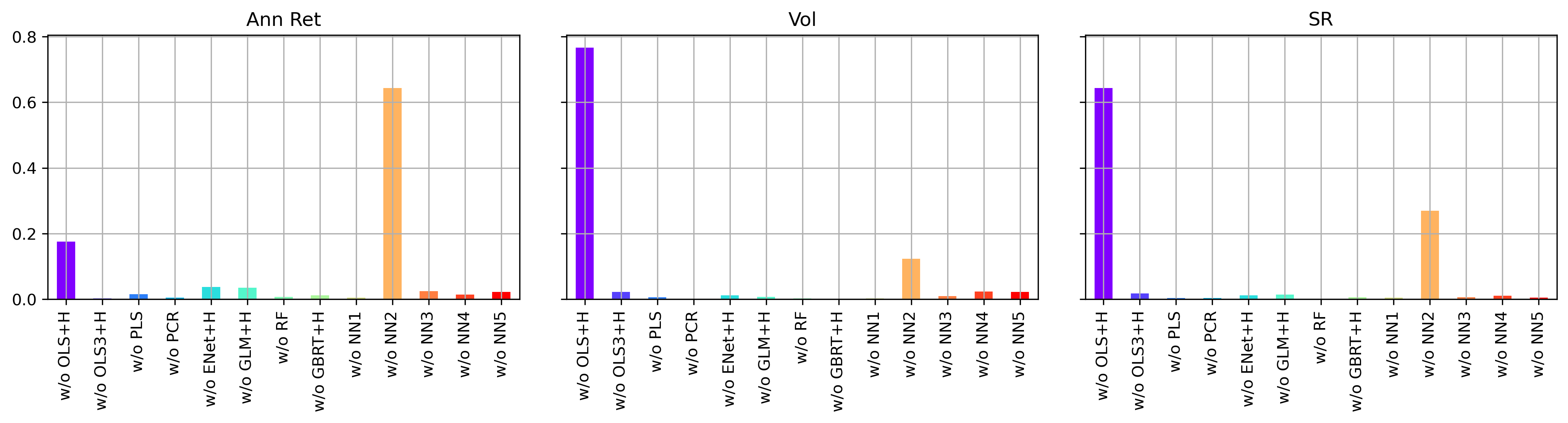
Figure 4: Experts’ Importance in the Bernstein Online Aggregation.

Note: The three graphs display experts importance computed over the out-of-sample period 1987-2016 based on three performance indicators: (1) annualised returns (Ann Ret), (2) volatility (Vol) and (3) annual Sharpe Ratio (SR). The importance indicator is obtained by measuring the difference between the performance of the mixture BOA considering all experts and the performance of the mixture when dropping a given expert, and then normalised to sum to one. Portfolios are equally weighted.

Expert specialisation

An individual expert can provide higher average returns on the test period than the aggregated Portfolio. This is an opportunity to improve the overall mixture by adding a slight variation of this best expert to the initial set of experts. To do so, if an expert obtains a lower loss than the aggregation, the expert is split into several new experts by re-calibrating it several times with new parameters or less inputs, as done in Devaine et al. (2013) for time series forecasting. This new set of experts is added to the initial set and a new aggregation is performed. Several methods to create new expert have been explored in the literature, such as Bagging, Specialisation, Temp Double Scale or Boosting (Gaillard and Goude, 2014).

Based on the analysis of experts’ importance, the neural network NN2 and OLS+H are split in several additional experts with the Bagging method, which gives better empirical results and is more computationally efficient. The method consists in training a bunch of identical models in parallel, where each model is trained by a random subset of the data. $K^{{}^{\prime}}=10$ new Ordinary Least Squared with Huber loss are trained as described in Section 3.1, and differ from the original OLS+H in the way they are fed during the training process (containing 80% of the original data). Models optimised with the Huber loss (noted “+H”) are trained by gradient descent which could be sensitive to local minima. Bagging allows to make the estimation more robust. Then the new strategies are added to the initial set of experts. Bagging with NN2 is done in a similar way.

Figure 5 shows annual Sharpe Ratios of the specialised aggregation with $K+2K^{{}^{\prime}}$ (here 33) experts. The extended PtfBOA outperforms all experts and reaches an annual Sharpe Ratio of 2.82, followed by the extended uniform mixture (2.79) and the original PtfBOA (2.77). More statistics can be found in Table C.14 in Appendix, in particular the extended PtfBOA keeps a low maximum monthly loss (7%). Expert specialisation brings Sharpe Ratio improvement while keeping the attractive properties (especially in terms of risk) of the original mixture.

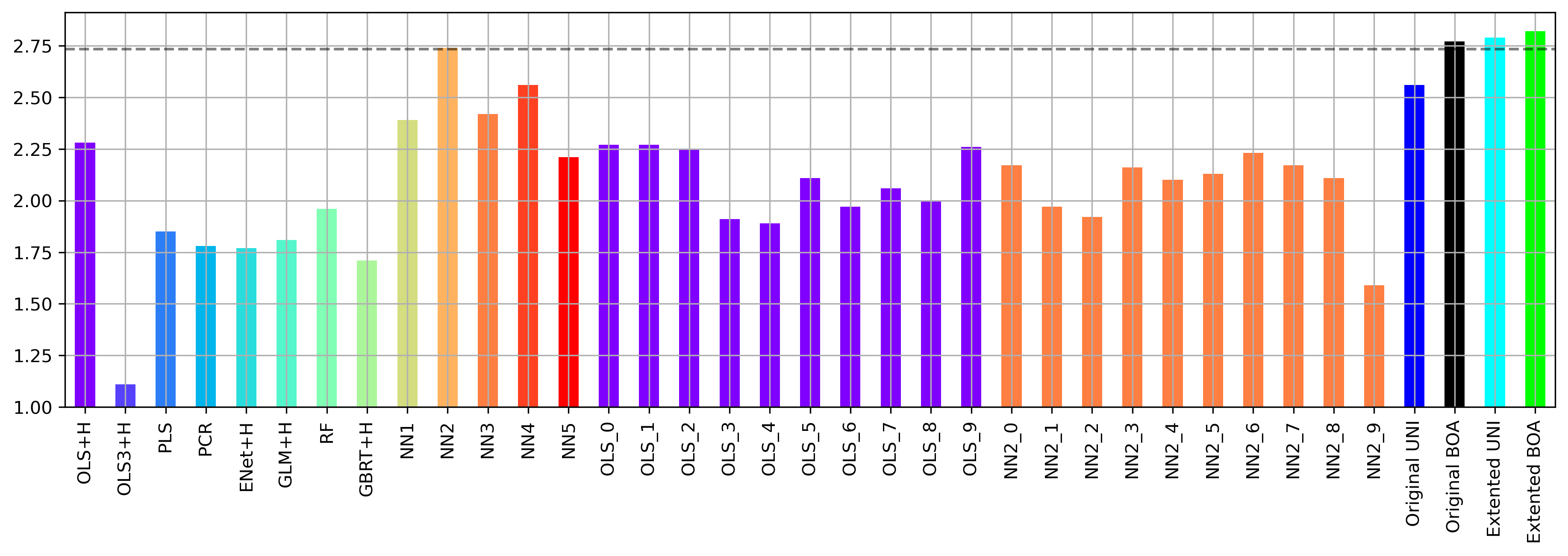
Figure 5: Portfolio Sharpe Ratios with Expert Specialisation.

Note: The graph plots the annual Sharpe Ratios of individual experts and aggregated portfolios, without (Original PtfUNI and PtfBOA) and with (Extended PtfUNI and PtfBOA) expert specialisation. Aggregation is performed with the initial set of $K$ experts plus $K^{{}^{\prime}}$ new specialised neural networks NN2 and $K^{{}^{\prime}}$ new specialised OLS+H. New forecasting models are trained by Bagging, then the corresponding portfolios are added in the initial set of experts. The dash line indicates the best expert Sharpe ratio. Portfolios are equally weighted.

Conclusion

A portfolio construction methodology based on a sequential aggregation of experts is presented. The strategies, called experts, lie on several forecasting algorithms such as linear models, tree-based models and neural networks. The aggregation performs online a convex combination of experts and adapts their weights dynamically according to their performance. The originality of the approach is to apply online aggregation directly on strategies, which is an easy way to improve portfolio allocation by combining heterogeneous strategies in a single algorithm. Online aggregation is particularly promising in finance where market conditions are known to be non-stationary. The aggregation is not computationally costly and considers directly the forecasts of the experts without any assumption on the data distribution and the expert models, allowing to consider any (potentially black-box) strategy. Moreover, the aggregation rules can easily be interpreted and are theoretically grounded. By building long-short strategy based on US stocks, numerical tests show that BOA aggregation offers higher performance than individual experts and simple mixtures. Betting on a single expert could be more attractive when one focuses on cumulative returns, but the aggregation oappears to be more robust over time and reduces the risk by deceasing significantly the maximum monthly loss and the maximum draw down. Further works could examine the design of specific loss functions for portfolio construction, leveraging the easy adaptation of the aggregation framework to alternative objectives.

Declarations

This work is supported by FiME, Laboratoire de Finance des Marchés de l’Énergie, and EDF Lab.

Conflict of interest The authors declare that they have no conflict of interest

Appendix

Appendix A Algorithms and Variables

In this section, some details are provided about the data and the parameters of the experts. All the variables used in this paper are exactly the same as Gu et al. (2020) and precisely described in the Table A.6 of its Appendix.

	OLS-OLS3+H	PLS	PCR	ENet+H
Huber Loss	$\xi=0.999$	-	-	$\xi=0.999$
Hyper Param		P=94	P=94	$\alpha\in(10e^{-4},10e^{-1})$
	Ensemble: 10			$\rho=0.5$
				Ensemble: 10
	GLM+H	RF	GBRT+H	NN1-NN5
Huber Loss	$\xi=0.999$	-	$\xi=0.999$	-
Hyper Param	$\alpha\in(10e^{-4},10e^{-1})$	Nb trees: 300	Nb trees: 1000	Batch size: 10000
	Ensemble: 10	Depth$\in(1,6)$	Depth$\in(1,2)$	Nb epoch: 100
		Bootstrap:True	Learning rate: {0.01,0.1}	Learning rate: 0.01
				Adam: Default
				Ensemble: 10
				Patience: 10
				L1 pen$\in(10^{-5},10^{-3})$

Table A.6: Description of Hyper-parameters of the Forecasting Models

Note: P=94 number of variables. OLS3+H only includes variables mom12m, size, bm. Hyper-parameters are optimised with the validation set.

Neural networks denoted NN1, NN2, NN3, NN4 and NN5 have hidden layer(s) of 32, (32,16), (32,16,8), (32,16,8,4) and (32,16,8,4,2) nodes respectively. ReLU activation function is used for each hidden layer, and regularisation methods include batch normalisation, learning rate shrinking (Adam), early stopping and ensemble. These setups are common standards in deep learning literature.

	OLS3	OLS7	OLS15		RF	NN3
%R2	0.16	0.19	0.19		0.19	0.45
SR	0.95	1.21	1.33		1.96	2.42
Turnover	0.49	0.48	0.56		0.92	1.20

Table A.7: OLS Benchmark Models.

Note: This table reports the performance of different Ordinary Least Squared benchmark models, as well as RF and NN3. The predictive R2 for stock return forecasting on test period, the Sharpe ratios of long-short strategies as well as their turnover are reported. OLS3 includes variables mom12m, size, bm, OLS7 adds acc, roaq, agr, egr, and OLS15 adds dy, mom36m, beta, retvol, turn, lev, sp. Models are trained on training and validation set data, as there is no hyper-parameters. This benchmark can be compared with Table A.11 of Gu et al. (2020).

The forecasting models are implemented in Python using scikit-learn Pedregosa et al. (2011) and tensorflow Abadi et al. (2015) packages. The online expert aggregation algorithm is computed with the R package OPERA (Gaillard et al., 2016).

Appendix B Metric Definitions

Metrics used in this paper are detailed here. Let be $y_{t}$ and $\hat{y}_{t}$ respectively the observed and the prediction values of one asset. Mean squared error (MSE) is defined by

$$\ell_{MSE}(y_{t},\hat{y}_{t})=\frac{1}{T}\sum^{T}_{t=1}(y_{t}-\hat{y}_{t})^{2},$$

and the Huber loss (HL) by

$$\ell_{HL}(y_{t},\hat{y}_{t};\xi)=\frac{1}{T}\sum^{T}_{t=1}H(y_{t}-\hat{y}_{t};\xi)\mbox{, where }H(x;\xi)=\begin{cases}x^{2}&\mbox{if }|x|\leq\xi\\ 2\epsilon|x|-\xi^{2}&\mbox{if }|x|\geq\xi.\\ \end{cases}$$

The Huber loss is less sensitive to outliers in the data distribution than MSE. $\xi$ determines the threshold from which it is less important to make an error. MSE and HL are used to train the forecasting models, aggregation optimises MSE. The R2 is used to evaluate the accuracy of asset return estimation:

$$R2=1-\frac{\sum^{T}_{t=1}(y_{t}-\hat{y_{t}})^{2}}{\sum^{T}_{t=1}y_{t}^{2}}.$$

The maximum draw down, 1-month maximum loss and portfolio turnover are defined by:

Max DD: $$\max_{0\leq t_{1}\leq t_{2}\leq T}(cr_{t_{1}}-cr_{t_{2}})$$

Max Loss: $$-\min_{0\leq t\leq T}r_{t}$$

Turnover: $$\frac{1}{T}\sum_{t=1}^{T}\left(\sum_{i}\left|w_{i,t+1}-w_{i,t}(1+r_{i,t+1})\right|\right)$$

where $cr_{t},r_{t}$ are the cumulative log return and the monthly excess return of a strategy at $t$ respectively, and $T$ the number of dates in the test period.

Appendix C Additional Tables and Figures

Performance of the forecasting models are reported in Table C.8 and Figure C.6. The R2 scores for predicting stock market returns show that the advantage of neural networks over linear models is not decisive. Moreover, while their accuracy is clearly convincing in some years, neural networks and random forest suffer from significant forecasting errors in other periods. These unstable scores complicate the choice of the most appropriate algorithm and light out why aggregation is appealing. Besides, on average the lowest market caps are better estimated than the top market cap stocks.

Figure C.7 illustrates annualised average returns of each expert’s long short strategy from 1987 to 2016. Up to 2002, strategies are profitable. However in 2003, several experts suffer from a breakout and are not able to retrieve the same performance afterward, even if models are re-calibrated each year. The variation in the rankings of the best experts from year to year emphasises the usefulness of aggregation techniques.

%R2	OLS	OLS3	PLS	PCR	ENet	GLM	RF	GBRT	NN1	NN2	NN3	NN4	NN5
	+H	+H			+H	+H		+H
All	0.19	0.13	0.22	0.25	0.23	0.24	0.19	0.09	0.48	0.69	0.45	0.37	0.44
Top	-0.20	0.13	-0.29	-0.12	-0.07	0.07	-0.07	-0.39	0.13	0.37	-0.23	0.18	0.12
Bot	0.30	0.34	0.47	0.48	0.42	0.39	0.52	0.42	0.94	1.19	0.92	0.84	0.88

Table C.8: %R2 Scores of the Forecasting Models

Note: The table reports the percent of R2 scores (1%R2 = 0.01 R2) of the thirteen forecasting models OLS+H, OLS3+H, PLS, PCR, ENet+H, GLM+H, RF, GBRT+H, NN1, NN2, NN3, NN4, and NN5 on the out-of-the-sample test period 1987-2016. All indicates all the US market universe. Top (resp. Bot) is the top 1000 (resp. bottom 1000) market capitalisation assets.

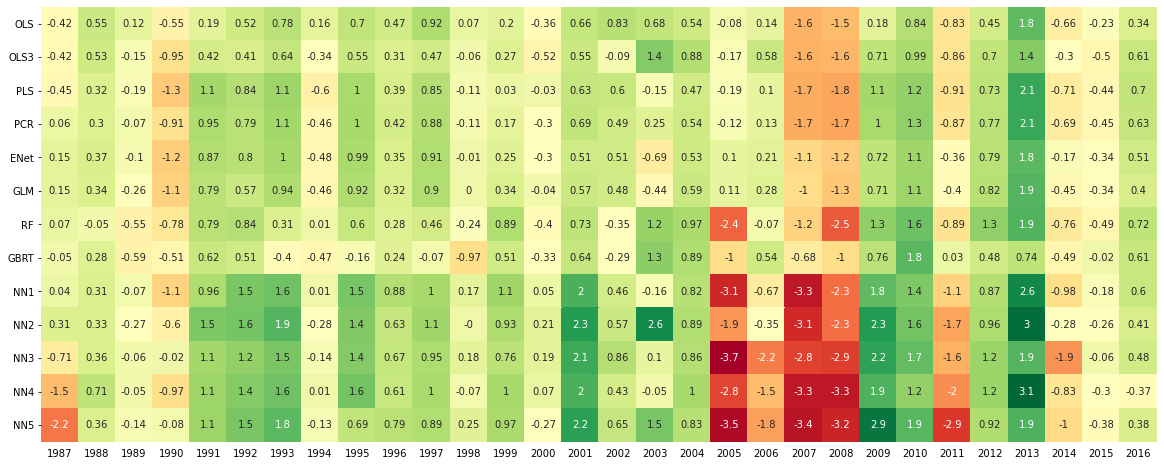
Figure C.6: %R2 Scores by Year of the Forecasting Models.

Note: The heatmap reports the percent of R2 scores (1%R2 = 0.01 R2) by year of the thirteen forecasting models OLS+H, OLS3+H, PLS, PCR, ENet+H, GLM+H, RF, GBRT+H, NN1, NN2, NN3, NN4, and NN5 on the out-of-the-sample test period 1987-2016.

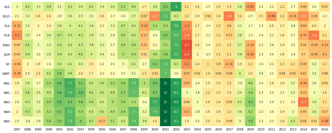
Figure C.7: Average Annualised Returns per Year of Portfolios.

Note: The expert portfolios are equally weighted and computed on the 1987-2016 test period. Experts include OLS+H, OLS3+H, PLS, PCR, ENet+H, GLM+H, RF, GBRT+H and the five neural networks (NN1-NN5). PtfBOA is the portfolio obtained with the Bernstein Online Aggregation and PtfUNI is an uniform mixture of the experts.

						OLS+H
Decile						Pred	Real	Std	SR
L						-1.35	-0.61	6.95	-0.30
2						-0.41	0.51	6.17	0.29
3						-0.05	0.77	5.61	0.48
4						0.39	0.97	5.23	0.64
5						0.70	1.09	5.07	0.74
6						0.98	1.21	5.05	0.84
7						1.28	1.30	5.05	0.89
8						1.61	1.49	5.23	0.98
9						2.04	1.70	5.45	1.08
H						2.88	2.11	6.00	1.22
H-L						4.49	2.99	4.50	2.28
	OLS3+H					PLS					PCR
Decile	Pred	Real	Std	SR		Pred	Real	Std	SR		Pred	Real	Std	SR
L	-0.19	0.44	6.77	0.23		-1.03	-0.12	7.22	-0.06		-0.9	-0.12	6.86	-0.06
2	0.16	0.72	5.48	0.46		-0.22	0.55	6.08	0.31		-0.15	0.58	6.0	0.33
3	0.38	0.98	4.83	0.7		0.2	0.79	5.55	0.49		0.24	0.81	5.37	0.52
4	0.58	1.00	4.49	0.77		0.52	0.89	5.21	0.59		0.54	0.9	5.21	0.6
5	0.77	0.98	4.43	0.77		0.82	0.96	5.05	0.66		0.82	0.99	5.12	0.67
6	0.94	0.96	4.79	0.69		1.10	1.07	5.16	0.72		1.08	1.03	5.20	0.69
7	1.11	1.06	5.31	0.69		1.40	1.17	5.18	0.79		1.35	1.18	5.27	0.78
8	1.28	1.22	6.09	0.70		1.74	1.39	5.25	0.92		1.66	1.42	5.27	0.94
9	1.49	1.23	6.44	0.66		2.17	1.65	5.35	1.07		2.04	1.64	5.58	1.02
H	1.81	1.94	8.08	0.83		3.00	2.18	5.87	1.29		2.79	2.11	6.14	1.19
H-L	2.26	1.76	5.47	1.11		4.29	2.57	4.79	1.85		3.96	2.50	4.85	1.78
	ENet+H					GLM+H					RF
Decile	Pred	Real	Std	SR		Pred	Real	Std	SR		Pred	Real	Std	SR
L	-0.86	-0.21	7.24	-0.1		-0.78	-0.29	7.41	-0.13		0.20	0.37	7.13	0.18
2	-0.16	0.61	6.28	0.34		-0.13	0.64	6.26	0.35		0.47	0.63	5.87	0.37
3	0.2	0.88	5.62	0.54		0.23	0.87	5.65	0.53		0.62	0.71	5.73	0.43
4	0.49	0.97	5.19	0.65		0.50	0.95	5.20	0.63		0.73	0.94	5.51	0.59
5	0.75	1.09	5.03	0.75		0.75	1.09	5.07	0.74		0.85	1.04	5.59	0.65
6	0.99	1.08	4.94	0.76		0.99	1.12	4.93	0.79		1.08	1.07	5.02	0.74
7	1.25	1.21	5.01	0.84		1.23	1.17	5.09	0.80		1.22	1.09	4.7	0.80
8	1.52	1.29	5.20	0.86		1.49	1.25	5.08	0.85		1.35	1.05	4.84	0.75
9	1.87	1.56	5.67	0.95		1.82	1.64	5.59	1.02		1.50	1.23	5.03	0.85
H	2.51	2.05	6.04	1.18		2.42	2.11	5.92	1.23		2.48	2.42	7.25	1.16
H-L	3.63	2.53	4.90	1.77		3.47	2.66	5.06	1.81		2.54	2.31	4.05	1.96
	GBRT+H					NN1					NN2
Decile	Pred	Real	Std	SR		Pred	Real	Std	SR		Pred	Real	Std	SR
L	-0.12	0.14	6.91	0.07		-1.46	-0.59	8.17	-0.25		-1.26	-0.63	8.07	-0.27
2	0.21	0.81	5.73	0.49		-0.33	0.46	6.34	0.25		-0.12	0.29	6.26	0.16
3	0.36	0.98	5.45	0.62		0.17	0.70	5.38	0.45		0.36	0.59	5.28	0.39
4	0.49	0.94	5.32	0.61		0.52	0.81	4.88	0.57		0.68	0.79	4.83	0.57
5	0.62	1.16	5.52	0.73		0.82	0.91	4.66	0.68		0.95	0.90	4.64	0.67
6	0.80	1.06	4.95	0.74		1.09	1.05	4.58	0.79		1.20	1.10	4.54	0.84
7	1.05	1.13	4.75	0.82		1.38	1.18	4.62	0.88		1.46	1.21	4.64	0.9
8	1.24	1.12	4.83	0.8		1.72	1.32	4.73	0.97		1.76	1.35	4.70	1.00
9	1.44	1.23	5.72	0.75		2.19	1.52	5.07	1.04		2.19	1.63	5.14	1.10
H	2.26	1.98	7.76	0.88		4.12	3.18	8.62	1.28		4.09	3.31	8.61	1.33
H-L	2.65	2.11	4.25	1.71		5.84	4.04	5.80	2.39		5.61	4.20	5.27	2.74
	NN3					NN4					NN5
Decile	Pred	Real	Std	SR		Pred	Real	Std	SR		Pred	Real	Std	SR
L	-1.54	-0.58	8.27	-0.24		-1.49	-0.61	8.36	-0.25		-0.87	-0.43	8.03	-0.19
2	-0.32	0.44	6.41	0.24		-0.17	0.40	6.38	0.22		0.16	0.49	6.22	0.27
3	0.20	0.68	5.31	0.44		0.38	0.70	5.35	0.45		0.55	0.81	5.27	0.53
4	0.55	0.75	4.91	0.53		0.74	0.80	4.84	0.57		0.82	0.92	4.72	0.68
5	0.85	0.88	4.71	0.65		1.03	0.92	4.61	0.69		1.04	1.04	4.65	0.78
6	1.11	1.07	4.59	0.81		1.30	1.08	4.54	0.83		1.24	0.98	4.60	0.74
7	1.39	1.19	4.63	0.89		1.58	1.22	4.55	0.93		1.45	1.16	4.61	0.87
8	1.70	1.38	4.72	1.01		1.9	1.35	4.74	0.99		1.71	1.26	4.74	0.92
9	2.15	1.58	5.05	1.09		2.36	1.53	5.10	1.04		2.09	1.39	5.31	0.90
H	4.12	3.16	8.43	1.30		4.48	3.16	8.33	1.31		4.10	2.92	8.81	1.15
H-L	5.92	4.01	5.70	2.42		6.23	4.03	5.56	2.58		5.23	3.62	5.64	2.21

Table C.9: Performance of Equally Weighted Portfolios by Decile.

Note: Performance on decile of each model for equally weighted portfolios. Rows L, H and HL stand for Low, High and High-minus-Low deciles respectively. Columns Pred, Real, Std, and SR are average predicted monthly returns (in %), average realised monthly returns (in %), realised monthly standard deviation (in %) and Sharpe ratio, respectively.

						OLS+H
Decile						Pred	Real	Std	SR
L						-1.13	-0.69	4.99	-0.48
2						-0.47	0.12	4.40	0.09
3						-0.15	0.31	3.95	0.28
4						0.09	0.46	3.68	0.43
5						0.30	0.54	3.58	0.53
6						0.50	0.63	3.56	0.62
7						0.71	0.70	3.58	0.68
8						0.94	0.84	3.73	0.78
9						1.23	1.00	3.87	0.89
H						1.82	1.29	4.27	1.04
H-L						3.20	2.24	3.34	2.32
	OLS3+H					PLS					PCR
Decile	Pred	Real	Std	SR		Pred	Real	Std	SR		Pred	Real	Std	SR
L	-0.32	0.07	4.95	0.05		-0.90	-0.32	5.30	-0.21		-0.82	-0.34	4.98	-0.23
2	-0.07	0.29	3.95	0.25		-0.33	0.16	4.38	0.13		-0.29	0.18	4.30	0.14
3	0.08	0.47	3.37	0.48		-0.04	0.34	3.96	0.29		-0.02	0.35	3.82	0.32
4	0.22	0.48	3.11	0.54		0.19	0.41	3.70	0.38		0.19	0.41	3.70	0.38
5	0.35	0.47	3.08	0.53		0.39	0.45	3.57	0.44		0.39	0.48	3.63	0.46
6	0.47	0.45	3.37	0.47		0.59	0.54	3.64	0.51		0.57	0.51	3.67	0.48
7	0.59	0.52	3.79	0.48		0.80	0.61	3.65	0.58		0.76	0.62	3.73	0.57
8	0.71	0.65	4.39	0.51		1.04	0.77	3.70	0.72		0.98	0.79	3.71	0.73
9	0.85	0.65	4.64	0.49		1.33	0.95	3.73	0.88		1.25	0.94	3.92	0.83
H	1.07	1.16	5.77	0.69		1.91	1.32	4.06	1.13		1.77	1.29	4.29	1.04
H-L	1.66	1.35	4.14	1.13		3.08	1.91	3.58	1.85		2.86	1.89	3.54	1.84
	ENet+H					GLM+H					RF
Decile	Pred	Real	Std	SR		Pred	Real	Std	SR		Pred	Real	Std	SR
L	-0.79	-0.39	5.23	-0.26		-0.73	-0.46	5.36	-0.30		-0.05	0.04	5.08	0.02
2	-0.3	0.20	4.47	0.15		-0.27	0.21	4.48	0.16		0.14	0.20	4.14	0.17
3	-0.04	0.40	3.98	0.35		-0.03	0.39	4.03	0.33		0.26	0.26	4.08	0.22
4	0.16	0.47	3.68	0.44		0.17	0.45	3.68	0.43		0.34	0.44	3.83	0.39
5	0.34	0.54	3.54	0.53		0.34	0.55	3.59	0.53		0.43	0.52	3.88	0.46
6	0.51	0.54	3.49	0.54		0.51	0.57	3.48	0.56		0.58	0.54	3.54	0.53
7	0.69	0.63	3.53	0.62		0.68	0.61	3.60	0.58		0.68	0.54	3.36	0.56
8	0.89	0.70	3.68	0.66		0.86	0.66	3.59	0.64		0.77	0.52	3.44	0.52
9	1.13	0.88	4.05	0.75		1.09	0.95	3.94	0.83		0.88	0.65	3.57	0.63
H	1.58	1.24	4.3	1.00		1.51	1.29	4.16	1.07		1.54	1.52	5.17	1.02
H-L	2.63	1.90	3.64	1.81		2.5	2.01	3.74	1.86		1.85	1.74	2.93	2.06
	GBRT+H					NN1					NN2
Decile	Pred	Real	Std	SR		Pred	Real	Std	SR		Pred	Real	Std	SR
L	-0.26	-0.13	4.81	-0.09		-1.21	-0.69	6.00	-0.40		-1.07	-0.70	5.89	-0.41
2	-0.03	0.34	3.96	0.29		-0.42	0.08	4.58	0.06		-0.27	-0.04	4.52	-0.03
3	0.07	0.47	3.86	0.42		-0.07	0.27	3.83	0.24		0.07	0.20	3.76	0.18
4	0.16	0.44	3.75	0.41		0.18	0.34	3.43	0.34		0.29	0.34	3.41	0.34
5	0.26	0.60	3.90	0.54		0.39	0.42	3.25	0.44		0.48	0.41	3.25	0.44
6	0.38	0.52	3.56	0.51		0.58	0.52	3.20	0.56		0.65	0.55	3.17	0.61
7	0.57	0.57	3.39	0.58		0.78	0.62	3.23	0.66		0.84	0.63	3.24	0.68
8	0.70	0.57	3.46	0.57		1.02	0.72	3.29	0.76		1.05	0.74	3.28	0.78
9	0.85	0.66	4.14	0.55		1.35	0.86	3.56	0.84		1.35	0.94	3.59	0.90
H	1.41	1.16	5.57	0.72		2.67	2.07	6.27	1.15		2.65	2.15	6.24	1.19
H-L	1.94	1.56	3.10	1.74		4.15	3.03	4.45	2.35		3.99	3.11	3.98	2.71
	NN3					NN4					NN5
Decile	Pred	Real	Std	SR		Pred	Real	Std	SR		Pred	Real	Std	SR
L	-1.28	-0.67	6.10	-0.38		-1.22	-0.68	6.12	-0.39		-0.80	-0.55	5.84	-0.33
2	-0.42	0.07	4.68	0.05		-0.30	0.04	4.63	0.03		-0.07	0.12	4.45	0.10
3	-0.05	0.25	3.79	0.23		0.09	0.26	3.79	0.24		0.20	0.35	3.75	0.33
4	0.20	0.30	3.48	0.30		0.34	0.34	3.40	0.34		0.39	0.42	3.33	0.44
5	0.40	0.40	3.31	0.42		0.54	0.42	3.23	0.45		0.54	0.51	3.28	0.54
6	0.59	0.53	3.21	0.58		0.73	0.54	3.18	0.58		0.68	0.46	3.21	0.50
7	0.78	0.62	3.21	0.67		0.93	0.64	3.19	0.69		0.83	0.60	3.21	0.65
8	1.00	0.76	3.25	0.81		1.16	0.74	3.32	0.78		1.01	0.67	3.30	0.70
9	1.32	0.91	3.51	0.90		1.48	0.87	3.56	0.84		1.28	0.76	3.74	0.70
H	2.66	2.04	6.04	1.17		2.92	2.05	6.02	1.18		2.65	1.86	6.40	1.01
H-L	4.20	2.98	4.31	2.39		4.40	3.00	4.13	2.51		3.71	2.68	4.27	2.17

Table C.10: Performance of Value Weighted Portfolios by Decile.

Note: Performance on decile of each model for value weighted portfolios. Rows L, H and H-L stand for Low, High and High-minus-Low deciles respectively. Columns Pred, Real, Std, and SR are average predicted monthly returns (in %), average realised monthly returns (in %), realised monthly standard deviation (in %) and Sharpe ratio, respectively.

	OLS	OLS3	PLS	PCR	ENet	GLM	RF	GBRT	NN1	NN2	NN3	NN4	NN5
	+H	+H			+H	+H		+H
	Equally Weighted
Ann Ret	0.36	0.21	0.31	0.30	0.30	0.32	0.28	0.25	0.48	0.50	0.48	0.48	0.43
Vol	0.16	0.19	0.17	0.17	0.17	0.18	0.14	0.15	0.20	0.18	0.20	0.19	0.20
SR	2.28	1.11	1.85	1.78	1.77	1.81	1.96	1.71	2.39	2.74	2.42	2.56	2.21
Skew	0.52	0.77	0.14	0.46	-0.05	-0.26	0.97	1.72	2.18	2.27	1.69	1.75	2.40
Kurt	4.36	17.89	7.96	7.50	7.42	8.63	7.03	12.63	19.44	13.94	11.12	11.47	19.56
Max DD	0.25	0.63	0.44	0.31	0.40	0.40	0.23	0.24	0.28	0.17	0.29	0.23	0.47
Max Loss	0.13	0.36	0.23	0.20	0.22	0.27	0.17	0.16	0.28	0.16	0.23	0.22	0.23
Turnover	1.26	1.50	1.15	1.27	1.28	1.36	0.92	1.25	1.24	1.23	1.20	1.20	1.15
	Value Weighted
Ann Ret	0.27	0.16	0.23	0.23	0.23	0.24	0.21	0.19	0.36	0.37	0.36	0.36	0.32
Vol	0.12	0.14	0.12	0.12	0.13	0.13	0.10	0.11	0.16	0.14	0.15	0.14	0.15
SR	2.29	1.13	1.84	1.83	1.79	1.84	2.04	1.72	2.33	2.67	2.37	2.48	2.16
Skew	0.84	0.82	0.16	0.62	0.13	-0.21	1.28	1.89	2.39	2.48	1.87	1.90	2.71
Kurt	5.30	23.68	9.14	7.84	7.58	9.78	6.52	14.23	23.00	16.41	13.35	13.26	24.58
Max DD	0.16	0.51	0.36	0.21	0.28	0.33	0.16	0.20	0.23	0.14	0.24	0.19	0.38
Max Loss	0.09	0.30	0.19	0.14	0.16	0.22	0.10	0.12	0.23	0.13	0.19	0.18	0.19
Turnover	1.05	1.33	1.02	1.06	0.97	1.07	0.51	0.67	0.66	0.60	0.69	0.55	0.52

Table C.11: Statistical Performance of Expert Portfolios.

Note: Statistical performance of equally and value weighted portfolios. Columns Ann Ret, Vol, SR, Skew, Kurt, Max DD, Max Loss and Turnover stand for annualised average return, annualised volatility, annualised Sharpe ratio, skewness, kurtosis, maximum drawdown, 1-month maximum loss and portfolio turnover. The metrics are computed on the test period 1987-2016.

	Best Expert	Fixed Combination		Adaptative Mixture		Oracle
	NN2	PtfUNI	Best Convex	Best Convex	PtfBOA	Best Convex
			on Valid. Set	One-year Rolling
	Equally Weighted
Ann. Ret.	0.50	0.36	0.36	0.43	0.49	0.50
Vol.	0.18	0.14	0.16	0.16	0.18	0.17
SR	2.74	2.56	2.28	2.60	2.77	2.92
Skew.	2.27	1.19	0.52	1.65	3.11	2.90
Kurt.	13.94	10.17	4.36	10.58	19.63	17.93
Max DD	0.17	0.24	0.25	0.17	0.08	0.07
Max Loss	0.16	0.18	0.13	0.16	0.08	0.07
Turnover	1.23	1.22	1.26	1.22	1.23	1.24
	Value Weighted
Ann. Ret.	0.37	0.27	0.27	0.32	0.36	0.37
Vol.	0.14	0.11	0.12	0.12	0.13	0.13
SR	2.67	2.54	2.29	2.57	2.73	2.76
Skew	2.48	1.20	0.84	1.69	3.00	3.21
Kurt	16.41	10.73	5.30	8.95	18.85	22.20
Max DD	0.14	0.20	0.16	0.14	0.09	0.08
Max Loss	0.13	0.15	0.09	0.11	0.05	0.08
Turnover	0.52	0.82	1.05	0.75	0.79	0.73

Table C.12: Performance of Aggregated Portfolios.

Note: Columns Ann. Ret., Vol., Skew., Kurt., SR, Max DD, Max Loss and Turnover stand for annualised average return, volatility, skewness, kurtosis, annual Sharpe ratio, maximum drawdown, 1-month maximum loss and portfolio turnover. The metrics are computed on the test period 1987-2016. Expect for NN2, all the portfolios are convex combinations of the thirteen experts. The oracle is the best possible convex mixture on the test period and is unachievable in practice.

	OLS	OLS3	PLS	PCR	ENet	GLM	RF	GBRT	NN1	NN2	NN3	NN4	NN5
	+H	+H			+H	+H		+H
	Equally Weighted
PtfUNI	0.08	0.08	0.08	0.08	0.08	0.08	0.08	0.08	0.08	0.08	0.08	0.08	0.08
Best Convex on Valid. Set	1.00	0.00	0.00	0.00	0.00	0.00	0.00	0.00	0.00	0.00	0.00	0.00	0.00
Best Convex One-year Rolling	0.25	0.00	0.02	0.02	0.02	0.03	0.04	0.03	0.15	0.14	0.07	0.11	0.12
PtfBOA	0.23	0.01	0.00	0.00	0.01	0.02	0.00	0.00	0.09	0.44	0.08	0.07	0.03
Oracle	0.30	0.00	0.00	0.00	0.00	0.00	0.00	0.00	0.00	0.59	0.00	0.11	0.00
	Value Weighted
PtfUNI	0.08	0.08	0.08	0.08	0.08	0.08	0.08	0.08	0.08	0.08	0.08	0.08	0.08
Best Convex on Valid. Set	1.00	0.00	0.00	0.00	0.00	0.00	0.00	0.00	0.00	0.00	0.00	0.00	0.00
Best Convex One-Year Rolling	0.25	0.01	0.02	0.01	0.03	0.03	0.03	0.03	0.15	0.13	0.07	0.11	0.13
PtfBOA	0.38	0.01	0.00	0.00	0.01	0.01	0.00	0.00	0.06	0.39	0.05	0.06	0.02
Oracle	0.26	0.00	0.00	0.00	0.00	0.00	0.00	0.00	0.24	0.50	0.00	0.00	0.00

Table C.13: Average Weights of the Mixtures.

Note: Average weights of the mixture portfolios on the test period 1987-2016. PtfUNI, Best Convex on Valid. Set, Best Convex One-year Rolling, PtfBOA, Oracle indicate the uniform mixture, the best fixed convex combination on the last year of the validation set, the one-year rolling fixed combination, BOA and the oracle portfolio weights respectively. The rolling best convex and BOA are adaptive mixtures, the weight evolution of the rolling mixture is given in the graph. Oracle is the best possible convex mixture on the test period and is unachievable in practice.

Experts	Ann Ret	Vol	Skew	Kurt	SR	Max DD	Max Loss
NN2_0	0.37	0.16	1.27	7.46	2.27	0.19	0.18
NN2_1	0.40	0.18	1.00	7.31	2.27	0.25	0.25
NN2_2	0.38	0.17	1.06	7.34	2.25	0.35	0.22
NN2_3	0.39	0.20	0.77	8.97	1.91	0.42	0.26
NN2_4	0.37	0.20	0.55	10.19	1.89	0.83	0.29
NN2_5	0.37	0.17	1.41	7.89	2.11	0.19	0.10
NN2_6	0.40	0.20	1.15	8.89	1.97	0.51	0.22
NN2_7	0.36	0.18	2.83	22.44	2.06	0.23	0.14
NN2_8	0.39	0.19	2.39	22.49	2.00	0.76	0.26
NN2_9	0.39	0.17	1.22	10.61	2.26	0.41	0.22
OLS+H_0	0.33	0.15	0.12	5.05	2.17	0.33	0.16
OLS+H_1	0.32	0.16	0.22	6.54	1.97	0.24	0.23
OLS+H_2	0.30	0.16	-0.05	5.20	1.92	0.41	0.19
OLS+H_3	0.32	0.15	-0.30	7.40	2.16	0.26	0.26
OLS+H_4	0.32	0.15	-1.03	10.1	2.10	0.31	0.29
OLS+H_5	0.31	0.14	0.24	3.32	2.13	0.21	0.14
OLS+H_6	0.35	0.16	0.53	3.72	2.23	0.22	0.14
OLS+H_7	0.32	0.15	0.60	5.28	2.17	0.26	0.13
OLS+H_8	0.32	0.15	0.30	5.52	2.11	0.36	0.18
OLS+H_9	0.29	0.18	0.19	5.75	1.59	0.41	0.19
Extended UNI	0.36	0.13	1.13	8.15	2.79	0.19	0.12
Extended BOA	0.47	0.17	2.98	18.39	2.82	0.09	0.07

Table C.14: Performance of Specialised Expert Portfolios and Extended Mixtures.

Note: Columns Ann Ret, Vol, Skew, Kurt, SR, Max DD, Max Loss provide annualised mean return, volatility, Skewness, Kurtosis, annual sharpe ratio, maximum drawdown and 1-month maximum loss. Extended BOA includes the $K=13$ initial experts plus $K^{{}^{\prime}}=10$ new specialised neural networks NN2 and $K^{{}^{\prime}}=10$ new specialised OLS+H. Portfolios are equally weighted.

References

- Abadi et al. (2015) M. Abadi, A. Agarwal, P. Barham, E. Brevdo, Z. Chen, C. Citro, G. S. Corrado, A. Davis, J. Dean, M. Devin, S. Ghemawat, I. Goodfellow, A. Harp, G. Irving, M. Isard, Y. Jia, R. Jozefowicz, L. Kaiser, M. Kudlur, J. Levenberg, D. Mané, R. Monga, S. Moore, D. Murray, C. Olah, M. Schuster, J. Shlens, B. Steiner, I. Sutskever, K. Talwar, P. Tucker, V. Vanhoucke, V. Vasudevan, F. Viégas, O. Vinyals, P. Warden, M. Wattenberg, M. Wicke, Y. Yu, and X. Zheng. TensorFlow: Large-scale machine learning on heterogeneous systems, 2015. URL https://www.tensorflow.org/. Software available from tensorflow.org.
- Albuquerque et al. (2022) P. H. M. Albuquerque, Y. Peng, and J. P. F. d. Silva. Making the whole greater than the sum of its parts: A literature review of ensemble methods for financial time series forecasting. Journal of Forecasting, 41(8):1701–1724, 2022. doi: https://doi.org/10.1002/for.2894.
- Amat et al. (2018) C. Amat, T. Michalski, and G. Stoltz. Fundamentals and exchange rate forecastability with simple machine learning methods. Journal of International Money and Finance, 88:1–24, 2018.
- Atiya (2020) A. F. Atiya. Why does forecast combination work so well? International Journal of Forecasting, 36(1):197–200, 2020.
- Auder et al. (2016) B. Auder, M. Bobbia, J.-M. Poggi, and B. Portier. Sequential aggregation of heterogeneous experts for pm10 forecasting. Atmospheric Pollution Research, 7(6):1101–1109, 2016.
- Azoury and Warmuth (2001) K. S. Azoury and M. K. Warmuth. Relative loss bounds for on-line density estimation with the exponential family of distributions. Machine Learning, 43(3):211–246, 2001.
- Bai et al. (2010) Y. Bai, J. Sun, J. Luo, and X. Zhang. Forecasting financial time series with ensemble learning. 2010 International Symposium on Intelligent Signal Processing and Communication Systems, pages 1–4, 2010. doi: 10.1109/ISPACS.2010.5704751.
- Bates and Granger (1969) J. M. Bates and C. W. Granger. The combination of forecasts. Journal of the Operational Research Society, 20(4):451–468, 1969.
- Blackwell (1956) D. Blackwell. An analog of the minimax theorem for vector payoffs. Pacific Journal of Mathematics, 6(1):1 – 8, 1956.
- Breiman (1996) L. Breiman. Bagging predictors. Machine Learning, 24:123–140, 1996.
- Breiman (2001) L. Breiman. Random forests. Machine Learning, 45:5–32, 2001.
- Brown et al. (2005a) G. Brown, J. Wyatt, R. Harris, and X. Yao. Diversity creation methods: a survey and categorisation. Information Fusion, 6(1):5–20, 2005a.
- Brown et al. (2005b) G. Brown, J. L. Wyatt, P. Tino, and Y. Bengio. Managing diversity in regression ensembles. Journal of Machine Learning Research, 6(9), 2005b.
- Butaru et al. (2016) F. Butaru, Q. Chen, B. Clark, S. Das, A. W. Lo, and A. Siddique. Risk and risk management in the credit card industry. Journal of Banking & Finance, 72:218–239, 2016.
- Cesa-Bianchi and Lugosi (2003) N. Cesa-Bianchi and G. Lugosi. Potential-based algorithms in on-line prediction and game theory. Machine Learning, 51:239–261, 2003.
- Cesa-Bianchi and Lugosi (2006) N. Cesa-Bianchi and G. Lugosi. Prediction, Learning, and Games. Cambridge University Press, 2006.
- Debry and Mallet (2014) E. Debry and V. Mallet. Ensemble forecasting with machine learning algorithms for ozone, nitrogen dioxide and pm10 on the prev’air platform. Atmospheric Environment, 91:71–84, 2014.
- Devaine et al. (2013) M. Devaine, P. Gaillard, Y. Goude, and G. Stoltz. Forecasting electricity consumption by aggregating specialized experts. Machine Learning, 90(2):231–260, 2013.
- Freund et al. (1996) Y. Freund, R. E. Schapire, et al. Experiments with a new boosting algorithm. In ICML, volume 96, pages 148–156. Citeseer, 1996.
- Freund et al. (1997) Y. Freund, R. E. Schapire, Y. Singer, and M. K. Warmuth. Using and combining predictors that specialize. In Proceedings of The Twenty-ninth Annual ACM Symposium on Theory of Computing, pages 334–343, 1997.
- Freyberger et al. (2020) J. Freyberger, A. Neuhierl, and M. Weber. Dissecting characteristics nonparametrically. The Review of Financial Studies, 33(5):2326–2377, 2020.
- Gaillard and Goude (2014) P. Gaillard and Y. Goude. Forecasting electricity consumption by aggregating experts; how to design a good set of experts. Lecture Notes in Statistics: Modeling and Stochastic Learning for Forecasting in High Dimension, 06 2014. doi: 10.1007/978-3-319-18732-7_6.
- Gaillard et al. (2014) P. Gaillard, G. Stoltz, and T. van Erven. A second-order bound with excess losses. In M. F. Balcan, V. Feldman, and C. Szepesvári, editors, Proceedings of The 27th Conference on Learning Theory, volume 35 of Proceedings of Machine Learning Research, pages 176–196, Barcelona, Spain, 13–15 Jun 2014. PMLR.
- Gaillard et al. (2016) P. Gaillard, Y. Goude, L. Plagne, T. Dubois, B. Thieurmel, M. P. Gaillard, L. Rcpp, R. I. Rcpp, and R. Rdpack. Package OPERA, 2016.
- Gu et al. (2020) S. Gu, B. Kelly, and D. Xiu. Empirical asset pricing via machine learning. The Review of Financial Studies, 33(5):2223–2273, 2020.
- Hannan (1957) J. Hannan. Approximation to bayes risk in repeated play. Contributions to the Theory of Games, 3:97–139, 1957.
- Heaton et al. (2017) J. B. Heaton, N. G. Polson, and J. H. Witte. Deep learning for finance: deep portfolios. Applied Stochastic Models in Business and Industry, 33(1):3–12, 2017.
- Herbster and Warmuth (1998) M. Herbster and M. K. Warmuth. Tracking the best expert. Machine Learning, 32(2):151–178, 1998.
- Hutchinson et al. (1994) J. M. Hutchinson, A. W. Lo, and T. Poggio. A nonparametric approach to pricing and hedging derivative securities via learning networks. The Journal of Finance, 49(3):851–889, 1994.
- Khandani et al. (2010) A. E. Khandani, A. J. Kim, and A. W. Lo. Consumer credit-risk models via machine-learning algorithms. Journal of Banking & Finance, 34(11):2767–2787, 2010.
- Kozak et al. (2020) S. Kozak, S. Nagel, and S. Santosh. Shrinking the cross-section. Journal of Financial Economics, 135(2):271–292, 2020.
- Lewellen (2014) J. Lewellen. The cross section of expected stock returns. Critical Finance Review, 4(1):1–44, 2014.
- Lin et al. (2021) H. Lin, D. Zhou, W. Liu, and J. Bian. Learning multiple stock trading patterns with temporal routing adaptor and optimal transport. In Proceedings of the 27th ACM SIGKDD Conference on Knowledge Discovery & Data Mining, pages 1017–1026, 2021.
- Littlestone and Warmuth (1994) N. Littlestone and M. K. Warmuth. The weighted majority algorithm. Information and Computation, 108(2):212–261, 1994.
- Moritz and Zimmermann (2016) B. Moritz and T. Zimmermann. Tree-based conditional portfolio sorts: The relation between past and future stock returns. Available at SSRN 2740751, 2016.
- Mourtada and Maillard (2017) J. Mourtada and O.-A. Maillard. Efficient tracking of a growing number of experts. In International Conference on Algorithmic Learning Theory, pages 517–539. PMLR, 2017.
- Nowotarski and Weron (2018) J. Nowotarski and R. Weron. Recent advances in electricity price forecasting: A review of probabilistic forecasting. Renewable and Sustainable Energy Reviews, 81:1548–1568, 2018.
- Nti et al. (2020) I. K. Nti, A. F. Adekoya, and B. A. Weyori. A comprehensive evaluation of ensemble learning for stock-market prediction. Journal of Big Data, 7(1):1–40, 2020.
- Pedregosa et al. (2011) F. Pedregosa, G. Varoquaux, A. Gramfort, V. Michel, B. Thirion, O. Grisel, M. Blondel, P. Prettenhofer, R. Weiss, V. Dubourg, J. Vanderplas, A. Passos, D. Cournapeau, M. Brucher, M. Perrot, and E. Duchesnay. Scikit-learn: Machine learning in Python. Journal of Machine Learning Research, 12:2825–2830, 2011.
- Petropoulos et al. (2022) F. Petropoulos, D. Apiletti, V. Assimakopoulos, M. Z. Babai, D. K. Barrow, S. B. Taieb, C. Bergmeir, R. J. Bessa, J. Bijak, J. E. Boylan, et al. Forecasting: theory and practice. International Journal of Forecasting, 2022.
- Rapach et al. (2013) D. E. Rapach, J. K. Strauss, and G. Zhou. International stock return predictability: what is the role of the united states? The Journal of Finance, 68(4):1633–1662, 2013.
- Rasekhschaffe and Jones (2019) K. C. Rasekhschaffe and R. C. Jones. Machine learning for stock selection. Financial Analysts Journal, 75(3):70–88, 2019.
- Sadhwani et al. (2021) A. Sadhwani, K. Giesecke, and J. Sirignano. Deep learning for mortgage risk. Journal of Financial Econometrics, 19(2):313–368, 2021.
- Schapire (1990) R. E. Schapire. The strength of weak learnability. Machine Learning, 5:197–227, 1990.
- Stoltz (2005) G. Stoltz. Incomplete Information and Internal Regret in Prediction of Individual Sequences. PhD thesis, Université Paris Sud - Paris XI, 2005. URL https://tel.archives-ouvertes.fr/tel-00009759.
- Sun et al. (2018) S. Sun, Y. Wei, and S. Wang. Adaboost-lstm ensemble learning for financial time series forecasting. In Computational Science–ICCS 2018: 18th International Conference, Wuxi, China, June 11–13, 2018 Proceedings, Part III 18, pages 590–597. Springer, 2018.
- Taillardat et al. (2016) M. Taillardat, O. Mestre, M. Zamo, and P. Naveau. Calibrated ensemble forecasts using quantile regression forests and ensemble model output statistics. Monthly Weather Review, 144(6):2375–2393, 2016.
- Thorey et al. (2017) J. Thorey, V. Mallet, and P. Baudin. Online learning with the continuous ranked probability score for ensemble forecasting. Quarterly Journal of the Royal Meteorological Society, 143(702):521–529, 2017.
- Vovk (1997) V. Vovk. Competitive on-line linear regression. Advances in Neural Information Processing Systems, 10, 1997.
- Vovk (1998) V. Vovk. A game of prediction with expert advice. Journal of Computer and System Sciences, 56(2):153–173, 1998. ISSN 0022-0000. doi: https://doi.org/10.1006/jcss.1997.1556.
- Vovk (2006) V. Vovk. On-line regression competitive with reproducing kernel hilbert spaces. In International Conference on Theory and Applications of Models of Computation, pages 452–463. Springer, 2006.
- Vovk (1990) V. G. Vovk. Aggregating strategies. Proc. of Computational Learning Theory, 1990, page 371–386, 1990.
- Weng et al. (2018) B. Weng, L. Lu, X. Wang, F. M. Megahed, and W. Martinez. Predicting short-term stock prices using ensemble methods and online data sources. Expert Systems with Applications, 112:258–273, 2018.
- Wintenberger (2017) O. Wintenberger. Optimal learning with bernstein online aggregation. Machine Learning, 106(1):119–141, 2017.
- (55) WRDS. Wharton research data services. URL https://wrds-web.wharton.upenn.edu/wrds/.
- Yang et al. (2020) H. Yang, X.-Y. Liu, S. Zhong, and A. Walid. Deep reinforcement learning for automated stock trading: An ensemble strategy. In Proceedings of the first ACM International Conference on AI in Finance, pages 1–8, 2020.
- Yao et al. (2000) J. Yao, Y. Li, and C. L. Tan. Option price forecasting using neural networks. Omega, 28(4):455–466, 2000.