Bilingual Topic Models for Comparable Corpora

Abstract

Probabilistic topic models like Latent Dirichlet Allocation (LDA) have been previously extended to the bilingual setting. A fundamental modeling assumption in several of these extensions is that the input corpora are in the form of document pairs whose constituent documents share a single topic distribution. However, this assumption is strong for comparable corpora that consist of documents thematically similar to an extent only, which are, in turn, the most commonly available or easy to obtain. In this paper we relax this assumption by proposing for the paired documents to have separate, yet bound topic distributions. We suggest that the strength of the bound should depend on each pair’s semantic similarity. To estimate the similarity of documents that are written in different languages we use cross-lingual word embeddings that are learned with shallow neural networks. We evaluate the proposed binding mechanism by extending two topic models: a bilingual adaptation of LDA that assumes bag-of-words inputs and a model that incorporates part of the text structure in the form of boundaries of semantically coherent segments. To assess the performance of the novel topic models we conduct intrinsic and extrinsic experiments on five bilingual, comparable corpora of English documents with French, German, Italian, Spanish and Portuguese documents. The results demonstrate the efficiency of our approach in terms of both topic coherence measured by the normalized point-wise mutual information, and generalization performance measured by perplexity and in terms of Mean Reciprocal Rank in a cross-lingual document retrieval task for each of the language pairs.

1 Introduction

Extracting information from the ever growing amount of documents available in more than one language is one of the challenges of Natural Language Processing. Any important progress on this domain has a significant impact on many applications ranging from speech recognition and intelligent interfaces to machine translation.

Probabilistic topic models like Latent Dirichlet Allocation (LDA) [8] are a family of unsupervised models that when applied to monolingual collections uncover the latent themes underlying it. Following their success in the monolingual setting, they have been extended to the bilingual setting. The most representative bilingual topic model is illustrated in Figure 2(i) and is commonly called bilingual LDA (biLDA) [41, 15, 52]. It extends LDA and does not require any prior, language dependent linguistic knowledge but the input collection to be in the form of pairs of thematically aligned documents. Given the pairs, a fundamental hypothesis of biLDA is that the documents of a pair share a single per-document topic distribution $\theta$. This entails that the documents in a pair discuss exactly the same themes. Although reasonable for parallel corpora, whose pairs consist of documents that are translations, this assumption is strong for collections composed by pairs of comparable documents (e.g. [38]), that is documents similar to some extent only. Figure 1 illustrates an example of comparable documents written in English and Portuguese. As the English document is larger, one would expect it to cover more topics. Hence, having a shared topic distribution between those two documents is a strong assumption.

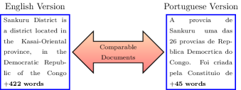
Figure 1: Motivating Example: excerpts from comparable Wikipedia documents. The English version is several times bigger than the Portuguese and one may reasonably assume it covers more topics.

In this paper we propose to extend bilingual topic models by relaxing the assumption of comparable documents sharing a single topic distribution. For this purpose, instead of a shared distribution we allow the documents of a pair to have two, separate, yet bound distributions. We suggest that the strength of the bound should depend on the semantic similarity of the documents of the pair. The estimation of this similarity for documents written in different languages is a task on itself. Instead of using dictionaries, which are one-to-one or one-to-$N$ discrete word associations and do not capture different levels of similarity, or machine translation systems, which are computationally expensive to develop, we propose to use cross-lingual word embeddings. Word embeddings are continuous vector representations of words that encode their semantic properties by projecting similar words close in a vector space [24, 39]. The cross-lingual embeddings, complementary to projecting similar words close in the semantic space for each language, project similar words across languages close in this space. Their potential has been previously shown for various tasks such as cross-lingual information retrieval [53].

Figure 2: The topic models used in this work. From left to right: (i) biLDA (ii) segBiLDA (iii) $\lambda$-biLDA (iv) $\lambda$-segBiLDA. The difference of biLDA and segBiLDA from their $\lambda-$ counterparts lies on the fact that the second have separate but bound topic distributions and the strength of binding is controlled by $\lambda$.

The questions we attempt to answer are twofold: $(Q1)$ How to better adapt bilingual topic models to comparable collections? $(Q2)$ Does this adaptation generalize well across different types of topic models? To address these questions, the paper proposes three contributions:

1. a novel approach that combines topic models with (shallow) neural networks for learning word embeddings allowing the former to extract latent distributions from comparable corpora,

2. the extension of biLDA and of a monolingual topic model that incorporates text structure in the form of boundaries of coherent text spans,

3. a systematic evaluation of the novel topic models on five comparable corpora where English are paired with French, German, Italian, Spanish and Portuguese documents.

We evaluate the topic models both on intrinsic and extrinsic tasks. Our results demonstrate the efficiency of our approach in terms of topic coherence measured by the normalized point-wise mutual information of the induced topics, generalization performance measured by calculating the perplexity of held-out documents, and in terms of Mean Reciprocal Rank in a cross-lingual document retrieval task for each of the language pairs. In the rest of the paper we provide a detailed discussion of these points.

2 Related Work

Our work lies in the intersection of the fields of multilingual topic modeling and cross-lingual word embeddings. We review the relevant literature starting with the work on multilingual topic models.

Multilingual Topic Models

There are two different lines of research in the multilingual topic modeling approaches with respect to the nature of the available training inputs. The first line assumes access or attempts to create linguistic resources such as dictionaries, in order to identify the topical links and alignments between the multilingual documents of a text corpus [9, 27, 58, 10]. The topic alignments between documents are not implicit in the input, and the models identify the topically relevant multilingual documents and the topic distributions while leveraging the available linguistic resources. For instance, [9] propose the multilingual topic model for unaligned text (MuTo) that discovers a parallelism in the documents of the corpus at the vocabulary level, while it assumes that similar themes are expressed in both languages. To perform the joint task of producing consistent topics in each of the two languages and then aligning them, the model uses dictionaries. JointLDA is a model with similar motivations, proposed in [27]. To cope with the multilingual setting, jointLDA also uses dictionaries but learns topics shared among the input languages. Those topics are distributions over the vocabulary terms of the multilingual corpus, and as a result, terms of different languages occur in a topic. Despite the advantages of such models, their requirements for several language-specific resources can be seen as a limitation.

The second, more flexible line of research, investigates topic modeling solely on the basis of the textual inputs. Those inputs, usually consist of text corpora with documents that are either parallel translations [60] or comparable translations of each other [46, 41, 14, 48]. Such topic models by not relying on any external resource are a better fit for unsupervised methods. The most representative model of this family is biLDA, which extends LDA in the bilingual [46, 41, 14] or the multilingual setting [29, 41]. The difference between the bi- or multilingual setting lies on the number of the input languages, which ranges from two to several.

The model we propose in this work belongs to this family of models as it assumes access to a corpus whose input documents form theme-aligned pairs. However, our model is more flexible as instead of assuming a single topic distribution per pair of documents, it uses two topic distributions that are linked with a binding mechanism that uses cross-lingual word embeddings to account for the level of similarity between the documents.

Cross-lingual Word Embeddings According to the distributional hypothesis [19, 24, 47], linguistic items such as words with similar distributions should have similar meanings. In other words, semantically similar words should have similar contextual distributions. The contextual information is usually induced assuming the context to be documents or sliding windows and is represented by populating word-context co-occurrence matrices. For words, different models that learn distributed representations have been recently proposed and those models are used as implementation models of the distributional hypothesis [49]. To this end, the distributed representations (also known as word embeddings) associate words with dense vectors, of dimension of a few hundreds to some thousands. A distributed representation of a symbol is a vector of features that characterize the meaning of the symbol and in our case a symbol is a word. The representation is a continuous $D$-dimensional vector and, therefore, compact in the sense that an exponential number of symbols (words) in the number of dimensions can be efficiently represented [49], compared, for instance, to the one-hot-encoding scheme that can only represent $D$ symbols when using $D$ dimensions.

Among different models, the skipgram model with negative sampling [39], has been shown to be efficient and effective in several applications [1]. Such a model is a function $f$ that projects a word $w$ in a $D$-dimensional space: $f(w)\in\mathbb{R}^{D}$, where $D$ is predefined. Although the model relies on a well-defined prediction task [5], it has been shown that it is implicitly factorizing a word-context matrix, whose cells are the pointwise mutual information (PMI) of the respective word and context pairs, shifted by a global constant [34, 35]. Despite the theoretical equivalence however, an advantage of the skipgram model compared to other models that factorize such matrices like Latent Semantic Indexing [26] is its ability to practically scale to huge amounts of data.

The skipgram model was initially proposed for the single language setting. However, motivated by the idea of having a single representation space shared by more languages, cross-lingual word embeddings models extended the idea in the bilingual and multilingual settings. The models can be grouped with regard to the approach used to align the cross-lingual embeddings. Models like [40] followed by [57, 33] for instance, begin by learning monolingual word embeddings and try to learn a linear transformation from one space to the other. Another way to learn cross-lingual embeddings [22, 18, 54] is by artificially generating multilingual documents by concatenating the documents of parallel or comparable corpora and then training existing monolingual models. Lastly, models like [37, 21] perform joint optimization of monolingual and cross-lingual losses. They can benefit from very big monolingual corpora for optimizing their monolingual objectives while relying on smaller corpora for optimizing their cross-lingual objective.

In this work we use Bilbowa [21]. It belongs in the family of models that jointly optimize monolingual and cross-lingual objectives. It extends the skipgram model for cross-lingual embeddings and trains directly on monolingual data. It uses a bilingual signal from a smaller set of raw-text sentence-aligned data to align the cross-lingual embeddings.

Combining Topic Models and Word Embeddings While topic models are trained to infer the per-word and per-document topic distributions, the skipgram model is trained by trying to predict the context of a word. Different efforts have attempted to extend the models by combining them. For instance, embeddings associate words with a single vector, which may be limiting for encoding the different meanings of polysemous words. This limitation motivated works that extend word embeddings with topic models. The purpose is for the topic models to uncover the different senses of a word, so that different embeddings can be derived for each sense [36, 12]. Such efforts attempt to produce better performing word embeddings.

In a relevant line of work, the purpose is to produce better topic models while taking advantage of the fact that text embeddings model semantic similarity. To this end, [45, 13, 59] extend topic models in order to encourage the models to group words that are a priori known to be semantically related into topics, where the a priori knowledge comes from training embeddings in large external corpora.

Our work belongs to this second line of research because we use word embeddings to improve the results of topic models. Differently from previous research though, word embeddings are used only to estimate the similarity of documents written in different languages. Also, our models are multilingual, while all previous work investigated the intersection of topic models and word embeddings in the monolingual setting using English.

3 Framework

Our primary goal in this work is to adapt the bilingual topic models for comparable corpora. To accomplish that we relax the assumption of paired documents having identical topic distributions. In the rest of this section, after presenting the notation, we briefly discuss biLDA in $\S$3.1. To illustrate how several classes of topic models can benefit by the adaptation to comparable corpora, we introduce a novel bilingual topic model that incorporates parts of the document’s structure ($\S$3.2). We, then, extend biLDA and the novel bilingual topic model for comparable corpora in $\S$3.3 and $\S$3.4.

$\ell_{1},\ell_{2}$	Input languages e.g., $\ell_{1}$=English, $\ell_{2}$=German
$d_{i},d_{i}^{\ell_{1}},d_{i}^{\ell_{2}}$	doc. pair $d_{i}$, whose aligned docs. are $d_{i}^{\ell_{1}}$, $d_{i}^{\ell_{2}}$
$\lambda_{i}$	The semantic similarity between $d_{i}^{\ell_{1}}$ and $d_{i}^{\ell_{2}}$
$V_{\ell}$	The size of the vocabulary in language $\ell$
$\Omega_{k,i}$	The number of words in $d_{i}$ assigned to topic $k$
$\theta_{i}$	Topic distribution of $d_{i}$
$\Psi_{k,w}$	The number of assignments of word $w$ to topic $k$
$\phi_{k}$	Word distribution for topic $k$
$s_{i,j}$	The $j^{th}$ segment of document $d_{i}$
$w_{i,j,k}$	The $k^{th}$ word of segment $s_{i,j}$
$N_{i}$	The number of words of document $d_{i}$
$N_{i,j}$	The number of words in segment $s_{i,j}$
$N_{i,j,w}$	The number of occurrences of word $w$ in $s_{i,j}$

Table 1: The notation used for the development of the topic models. Adding exponents $\ell_{1},\ell_{2}$ to the symbols of the lower part of the table (below the dashed line) stands for counts specific to $d_{i}^{\ell_{1}},d_{i}^{\ell_{2}}$.

The notation is summarized in Table 1. For consistency, we keep the symbols of previous work [56] to the extent of possible. We denote $\ell_{1}$ and $\ell_{2}$ the different languages present in a comparable corpus. As languages are handled symmetrically, for convenience we designate by $\ell\!\!\backslash$, the language different from language $\ell\in\{\ell_{1},\ell_{2}\}$. The inputs of the topic models are document pairs $d_{i}=(d_{i}^{\ell_{1}},d_{i}^{\ell_{2}})$, that consist of thematically aligned documents $d_{i}^{\ell_{1}}$ and $d_{i}^{\ell_{2}}$, written in $\ell_{1}$ and $\ell_{2}$. Depending on the model, documents are either represented as a bag-of-words, or as a bag-of-segments. Segments are text spans smaller than documents, for instance sentences, and are represented as a bag-of-words. Considering $\ell\in\{\ell_{1},\ell_{2}\}$, $s_{i,j}^{\ell}$ is the $j^{th}$ segment of document $d_{i}^{\ell}$. Segmented documents have a hierarchical structure: they are composed by segments that are composed by words in turn. Depending on the model, there may exist either a single $\theta_{i}$ topic distribution that captures the topics present in both documents of the pair $d_{i}$, or two, separate yet bound topic distributions $\theta_{i}^{\ell}$, $\theta_{i}^{\ell\!\!\backslash}$ that capture the topics of $d_{i}^{\ell}$ and $d_{i}^{\ell\!\!\backslash}$ respectively. The rest of the notation in Table 1 stands for count matrices or vectors used during inference.

3.1 The bilingual LDA

biLDA (Figure 2(i)) is a direct adaptation of LDA in the bilingual setting where a parallel collection is assumed to be the model’s input. Due to its effectiveness we use it as a reference in this work. biLDA assumes that the documents of an aligned pair $d_{i}$ have identical topic distributions (a single and shared $\theta_{i}$) and therefore discuss the same topics. Also, it expects the documents as a bag-of-words. Its generative story is as follows:

• for each topic $k\in[1,K]$: $\phi_{k}^{\ell_{1}}\sim Dir(\beta)$, $\phi_{k}^{\ell_{2}}\sim Dir(\beta)$

• for each document pair $d_{i}$:

  • sample $\theta_{i}\sim Dir(\alpha)$

  • for each language $\ell\in\{\ell_{1},\ell_{2}\}$

    • for each of the $N^{\ell}_{i}$ words:

      • sample $z\sim Mult(1,\theta_{i})$

      • sample $w\sim Mult(1,\phi^{\ell}_{z})$

The collapsed Gibbs sampling updates [52] for the topic of word $j$ of document $d_{i}$ is $\forall\ell\in\{\ell_{1},\ell_{2}\}$:

$$P\Big{(}z_{ij}^{\ell}=z_{k}|\bm{z}_{\neg{ij}}^{\ell},\bm{z}^{\ell\!\!\backslash},\bm{w}^{\ell},\bm{w}^{\ell\!\!\backslash},\alpha,\beta,\Big{)}\propto\frac{\Psi_{k,w,\neg ij}^{\ell}+\beta}{\Psi_{k,\cdot,\neg ij}^{\ell}+V_{\ell}\beta}[\Omega_{i,k,\neg ij}+\alpha]$$

A dot “$\cdot$” occurring in the subscript of a count variable, stands for the summation over the possible values of the element it replaces, i.e.,$\Psi_{k,\cdot,\neg ij}^{\ell}=\sum\limits_{w=1}^{V}\Psi_{k,w,\neg ij}^{\ell}$. Also, $\neg$ stands for excluding the counts of the particular variable with respect to a segment, e.g., $\neg ij$ excludes the counts of the $j$-th word of $d_{i}^{\ell}$. Further, $Dir(\alpha)$ stands for a sample from a Dirichlet distribution with prior $\alpha$ and $Mult(M,\theta)$ stands for $M$ samples from a Multinomial distribution parametrized by $\theta$.

For biLDA, as well as for the models we present next, we consider the Dirichlet hyperparameters $\alpha\in\mathbb{R}^{K}$ and $\beta\in\mathbb{R}^{V}$ to have fixed values, implying symmetric priors. Extending the models to asymmetric priors or even learning their values could be done as in [3] for example. Also, as commonly done we omit from the generative stories the steps where the sizes of segments or documents are sampled as their sizes are observed during inference. As noted, biLDA uses a bag-of-words representation; next we present an extension that uses a more complex document representation.

3.2 Text structure incorporation

In this section, we propose segment-BiLDA (segBiLDA) that incorporates prior knowledge of text structure using a more complex document representation than bag-of-words. Although important for inference, the bag-of-words assumption is limiting. In fact, previous research in the single language domain showed the benefits of similar extensions: Wang et al. [55] proposed a model that handles bigrams as a single token or as two unigrams depending on the topic, Lau et al. [32] modeled frequent bigrams as separate tokens, Balikas et al. [4] proposed to incorporate sentence boundaries to LDA, while Boyd et al. [11] incorporated parse trees . These important contributions focused on the monolingual setting and used English texts for empirical evaluation. Here, we extend topic models to account for text structure in the bilingual case.

For our subsequent analysis, we define coherent text segments to be contiguous words of a document that are topically coherent. A topically coherent text segment refers to a segment whose constituent words discuss a single or very few related themes. For instance, one would expect frequent bigrams like “information retrieval” or even short sentences to be topically coherent as they generally convey a simple message. We model this property with (segBiLDA), which is illustrated in Figure 2(ii). segBiLDA assumes that the input text is segmented a priori and incorporates the boundaries of segments in its generative story:

• for each topic $k\in[1,K]$: $\phi_{k}^{\ell_{1}}\sim Dir(\beta)$, $\phi_{k}^{\ell_{2}}\sim Dir(\beta)$

• for each document pair $d_{i}$:

  • sample $\theta_{i}\sim Dir(\alpha)$

  • for each language $\ell\in\{\ell_{1},\ell_{2}\}$

    • for the $j$ segment ($1\leq j\leq S^{\ell}$ ):

      • sample $z\sim Mult(1,\theta_{i})$

      • sample segment words:
        $(w_{1}\ldots w_{N_{i,j}^{\ell}})\sim Mult(N^{\ell}_{i,j},\phi^{\ell}_{z})$

The important difference of biLDA from segBiLDA (Figures 2(i) and 2(ii)) lies in the addition of the segment’s plate. A topic is sampled per segment, and every word of a segment is associated with it. The segment boundaries limit the number of topics that appear in the segment to be equal to one. As in biLDA though, words remain the document units and this single topic is associated with each word of the segment. Therefore, comparing the models on measures like perplexity that are calculated at the word level is fair. To infer these topics we propose a collapsed Gibbs sampling approach, that $\forall\ell\in\{\ell_{1},\ell_{2}\}$, samples topics from:

$$P(z_{s_{i,j}}^{\ell}=z_{k}|\bm{z}_{\neg s_{ij}}^{\ell},\bm{z}^{\ell\!\!\backslash},\bm{w}^{\ell},\bm{w}^{\ell\!\!\backslash},\alpha,\beta)\propto[\Omega_{i,k,\neg s_{i,j}}+\alpha]\times$$

$$\frac{\prod\limits_{w\in s_{ij}^{\ell}}(\Psi_{k,w,\neg s_{ij}}^{\ell}+\beta)\cdots(\Psi_{k,w,\neg s_{ij}}^{\ell}+\beta+(N_{i,j,w}^{\ell}-1))}{(\Psi_{k,\cdot,\neg s_{ij}}^{\ell}+\beta V_{\ell})\cdots(\Psi_{k,\cdot,\neg s_{ij}}^{\ell}+\beta V_{\ell}+(N_{i,j}^{\ell}-1))}$$ (1)

For convenience, we discuss the derivation of Eq. (1) in the Appendix. In Eq. (1), the product appearing in the numerator of the second term results from the bag-of-words assumption for the words of segments. The (possibly multiple) occurrences of a word $w$ in a segment $s_{i,j}^{\ell}$, generated by the topic $k$, are taken into account by the factor $(\Psi_{k,w,\neg s_{ij}}^{\ell}+\beta)$, which is incremented by one for every other occurrence of the word after the first. For example, if word $w$ appears twice in $s_{i,j}^{\ell}$, then $N_{i,j,w}^{\ell}=2$, and the factor $(\Psi_{k,w,\neg s_{ij}}^{\ell}+\beta)(\Psi_{k,w,\neg s_{ij}}^{\ell}+\beta+1)$ denotes the contribution of the occurrences of the word to the probability that $s_{i,j}^{\ell}$ is generated by the topic $k$. This way, every word of the segment contributes to the probability of sampling a particular topic. Similarly, the denominator acts as a normalization term. The progressive increase of its values can also be explained intuitively: given the bag-of-words assumption of words within a segment, the product normalizes the probability of assigning the topic $k$ to a word of the segment, given that the previous words have also been assigned to this topic. Notice, that if the size of the segment is 1, the model as well as the sampling equations reduce to biLDA.

The bag-of-words assumption in biLDA results in a joint distribution of random variables (here topics) being invariant to any permutation of the variables (exchangeability). This holds for segBiLDA only locally, within segments. Globally, within a document, words are not exchangeable as the segment boundaries are utilized. While in biLDA the topics of words are conditionally independent given the document’s topic distribution, for segBiLDA they are not, as they also depend on the rest of the segment’s words.

Previous work in the monolingual case suggested to incorporate various types of text structure to topic models ranging from $n$-grams to parse trees. segBiLDA can be considered an extension of the model of Balikas et al. [4] in the bilingual setting. Rather than extending more complex models like Boyd’s [11] that may require parsing the documents, we opt for segBiLDA due to the variety of segments it can handle. For instance, one can use linguistically motivated segmentation approaches like sentence tokenization or statistically motivated segmentation approaches like frequent $n$-grams with the same model. Furthermore, these segmentation approaches can be accomplished efficiently and accurately across a wide range of languages without resorting to complex linguistic analysis tools like parsers.

3.3 Multilingual topic Extraction

biLDA and segBiLDA assume a single topic distribution for the documents of a pair, which as illustrated in Figure 1 is a string assumption for comparable documents. Apart from that, the motivations for adapting the bilingual topic models to comparable corpora lie on two facts: on one hand, comparable corpora are more common and easy to obtain or to construct than parallel ones, which require additional linguistic knowledge and tools. On the other hand, recent advances on cross-lingual word embeddings resulted in methods that can be directly used to estimate the semantic similarity of documents written in different languages. The latter facilitates the application of our method to various pairs of languages without expensive resources.

For comparable corpora, we first propose the $\lambda$-biLDA model, whose graphical model is shown in Figure 2(iii). In this case, instead of having a single, shared topic distribution we have a topic distribution per language shown as $\theta^{\ell_{1}}$ and $\theta^{\ell_{2}}$ in the figure. However, these distributions are bound between them. To model naturally the possible levels of dependence between $\theta^{\ell_{1}}$ and $\theta^{\ell_{2}}$ we need a binding mechanism flexible enough to model the two extreme conditions: total independence between the topic distributions of the aligned documents that should result in two distinct LDA models (one per language), and a complete dependence between them (identical topic distributions) which should result in biLDA. Similar dependence mechanisms were previously explored under the setting of streaming documents [2], where topic distributions of earlier documents affect the distributions of later documents.

The generative process for $\lambda$-biLDA is as follows:

• for each topic $k\in[1,K]$: $\phi_{k}^{\ell_{1}}\sim Dir(\beta)$, $\phi_{k}^{\ell_{2}}\sim Dir(\beta)$

• for each document pair $d_{i}=(d_{i}^{\ell_{1}},d_{i}^{\ell_{2}})$:

  • sample $\lambda_{i}$ with respect to $d_{i}$

  • sample $\theta_{i}^{\ell_{1}}\sim Dir(\alpha+\lambda_{i}\theta_{i}^{\ell_{2}})$, $\theta_{i}^{\ell_{2}}\sim Dir(\alpha+\lambda_{i}\theta_{i}^{\ell_{1}})$

  • for language $\ell\in\{\ell_{1},\ell_{2}\}$

    • for each of the words $N^{\ell}$:

      • sample $z\sim Mult(1,\theta_{i}^{\ell})$

      • sample $w\sim Mult(1,\phi^{\ell}_{z})$

The central idea is that the topic distributions of documents in one language depend on the topic distributions of documents in the other language via a binding mechanism that generates $\theta^{\ell}$ with a Dirichlet distribution depending on $\theta^{\ell\!\!\backslash};\theta^{\ell}|\theta^{\ell\!\!\backslash}\sim Dir(\alpha+\lambda_{i}\theta_{i}^{\ell\!\!\backslash})$ and vice-versa. Note that from the Hammersley-Clifford theorem [23], fixing the two conditional distributions $\theta^{\ell_{1}}|\theta^{\ell_{2}}$ and $\theta^{\ell_{2}}|\theta^{\ell_{1}}$ defines in an unique way the distribution of $(\theta^{\ell_{1}},\theta^{\ell_{2}})$ which implies that our generative process is well-defined.

For inferring the topics of the observed words we propose a Gibbs sampling approach, whose derivation is given in the Appendix. The update equations for the topics of the words are then $\forall\ell\in\{\ell_{1},\ell_{2}\}$:

$$P\Big{(}z_{i,j}^{\ell}=z_{k}|\bm{z}_{\neg{i,j}}^{\ell},\bm{w}^{\ell},\alpha,\beta,\lambda_{i},\theta^{\ell\!\!\backslash}\Big{)}\propto$$

$$\frac{\Psi_{k,w,\neg i,j}^{\ell}+\beta}{\Psi_{k,\cdot,\neg i,j}^{\ell}+V_{\ell}\beta}\cdot[\Omega_{i,k,\neg i,j}^{\ell}+\alpha+\lambda_{i}\theta_{d,k}^{\ell\!\!\backslash}]$$ (2)

Gibbs sampling algorithms obtain posterior samples by sweeping though each block of variables and sampling from their conditional, while the remaining blocks are fixed. In practice, the algorithm initializes randomly the topics of words. Then, during the Gibbs iterations and until convergence, sampling topics for words of $\ell$ assumes the distribution of $\theta^{\ell\!\!\backslash}$ fixed, and hence can be accessed as assumed by the generative story.

In Eq. (2), $\lambda_{i}$ captures the dependency between the topic distributions of the documents of $d_{i}$. We use cross-lingual word embeddings for its estimation. We use the average (avg) compositional function of meaning, which was shown to be robust and effective [43, 7]. Having the vectors of the document pair $d_{i}=(d_{i}^{\ell_{1}},d_{i}^{\ell_{2}})$ in the embedded space, we then estimate $\lambda_{i}$ using the cosine similarity. Calculated in this way, $\lambda_{i}\in[-1,1]$ and since $\theta_{d,k}\in[0,1]$ it follows for the second term of Eq. 2 that $\Omega_{i,k,\neg i,j}^{\ell}>>\lambda_{i}\theta_{d,k}$, which results in negligible impact for $\lambda_{i}\theta_{d,k}$. To circumvent that we use:

$$\lambda_{i}^{\prime}=\lambda_{i}\times|N_{i}^{\ell\!\!\backslash}|=\Omega^{\ell\!\!\backslash}_{d,k}$$ (3)

Notice that incorporating Eq. (3) to Eq. (2) has as an additional advantage the capacity to generalize previous models. In particular, it follows that biLDA becomes a special case of $\lambda$-MuLDA with $\lambda=1$ (complete dependency where $\theta^{\ell}$ and $\theta^{\ell\!\!\backslash}$ are the same topic distributions). Also, when $\lambda=0$ (case of independence) we have two distinct LDAs, one per language.

3.4 Combining the two models

To this point, we proposed segBiLDA that incorporates the boundaries of coherent segments like sentences, and $\lambda$-biLDA, that assumes bound topic distributions for the paired documents in the two languages. The two models can be combined: $\lambda$-segBiLDA assigns consistent topics in the words of the segments of the documents and also assumes different topic distributions for each language.

We illustrate $\lambda$-segBiLDA in Figure 2(iv). We omit the generative story, since it is a direct combination of the generative stories of segBiLDA and $\lambda$-biLDA. The inference process is given by the following equation, whose derivation is given in the Appendix. To sample the topics of segments from the conditional distribution for $\forall\ell\in\{\ell_{1},\ell_{2}\}$:

$$P\Big{(}z_{i,j}^{\ell}=z_{k}|\bm{z}_{\neg{i,j}}^{\ell},\bm{w}^{\ell},\alpha,\beta,\lambda_{i},\theta^{\ell\!\!\backslash}\Big{)}\propto[\Omega_{i,k,\neg s_{i,j}}^{\ell}+\alpha+\lambda_{i}\Omega_{d,k}^{\ell\!\!\backslash}]\times$$

$$\frac{\prod\limits_{w\in s_{ij}^{\ell}}(\Psi_{k,w,\neg s_{ij}}^{\ell}+\beta)\cdots(\Psi_{k,w,\neg s_{ij}}^{\ell}+\beta+(N_{i,j,w}^{\ell}-1))}{(\Psi_{k,\cdot,\neg s_{ij}}^{\ell}+\beta V_{\ell})\cdots(\Psi_{k,\cdot,\neg s_{ij}}^{\ell}+\beta V_{\ell}+(N_{i,j}^{\ell}-1))}$$ (4)

Notice how both assumptions are relaxed is this model: the first term of the result (discussed in the Appendix) shown in Eq. (4) accounts for the topic dependence between the paired documents, while the second incorporates the segment boundaries.

4 Experimental Framework

	Full Dataset			Topic Modeling Subsets
Dataset	$D$	$N$	$V$	$D$	$N$	$V$
Wiki${}^{\text{En}}_{\text{En-Fr}}$	937,991	259M	619,056	10,000	2.55M	33,925
Wiki${}^{\text{Fr}}_{\text{En-Fr}}$	937,991	159M	466,423	10,000	1.64M	26,604
Wiki${}^{\text{En}}_{\text{En-Ge}}$	849,955	391M	599,233	10,000	2.54M	33,198
Wiki${}^{\text{Ge}}_{\text{En-Ge}}$	849,955	391M	894,798	10,000	1.81M	44,898
Wiki${}^{\text{En}}_{\text{En-It}}$	732,416	200M	519,897	10,000	2.55M	33,934
Wiki${}^{\text{It}}_{\text{En-It}}$	732,416	125M	360,760	10,000	1.56M	25,436
Wiki${}^{\text{En}}_{\text{En-Es}}$	672,094	198M	497,805	10,000	2.82M	35,156
Wiki${}^{\text{Es}}_{\text{En-Es}}$	672,094	135M	355,677	10,000	1.86M	25,796
Wiki${}^{\text{En}}_{\text{En-Pt}}$	540,467	160M	428,293	10,000	2.86M	34,687
Wiki${}^{\text{Pt}}_{\text{En-Pt}}$	540,467	61M	222,547	10,000	1.9M	19,347

Table 2: Data used for evaluating topic coherence (left) and topic modeling (right) purposes. The names signify the language pair and the language that the statistics correspond to. For instance, Wiki${}^{\text{en}}_{\text{en-fr}}$ are the English documents of the En-Fr corpus.

BiLDA						segBiLDAs
Topic 3 [City]		Topic 5 [Sports]		Topic 8 [Art]		Topic 3 [City]		Topic 5 [Sports]		Topic 8 [Art]
En	Fr	En	Fr	En	Fr	En	Fr	En	Fr	En	Fr
city	commun	team	championnat	music	group	citi	vill	team	championnat	film	the
popul	situ	play	club	album	album	popul	situ	play	club	releas	of
town	vill	first	premi	releas	titre	area	commun	first	premi	also	film
area	référent	game	coup	song	the	town	part	world	match	album	and
locat	région	player	match	record	and	locat	grand	leagu	coup	first	sort
$\lambda$-BiLDA						$\lambda$-segBiLDAs
Topic 3 [City]		Topic 5 [Sports]		Topic 8 [Art]		Topic 3 [City]		Topic 5 [Sports]		Topic 8 [Art]
En	Fr	En	Fr	En	Fr	En	Fr	En	Fr	En	Fr
citi	commun	team	championnat	music	group	popul	situ	team	championnat	film	the
popul	vill	play	club	album	premi	city	espec	play	premi	releas	of
town	situ	first	premi	release	sort	also	vill	first	club	album	film
refer	villag	player	coup	song	the	area	part	world	coup	also	and
area	référent	game	saison	record	album	town	grand	leagu	saison	song	sort

Table 3: For each of the topic models we present three topics: City, Sports, Art for the “En-Fr” Wikipedia corpus. Notice the strong intra-semantic (words within a topic) and inter-semantic (topics across languages) coherence.

The comparable corpora In order to evaluate the proposed models, we perform a series of evaluation tasks using Wikipedia documents in five language pairs as our comparable corpora. The language pairs are English-French (En-Fr), English-German (En-Ge), English-Italian (En-It), English-Spanish (En-Es) and English-Portuguese (En-Pt). Table 2 shows the basic statistics of these datasets. For topic modeling purposes we have sampled subsets from the full datasets (right part of the table) consisting of 10,000 documents for each pair. Since the sampling was random, it is not the same 10,000 English documents used for every language pair. Notice in the table that for each pair English is the language with the most words ($N$), which was expected since often Wikipedia lemmas are first written in English and then translated to other languages. This is also why Wikipedia is a suitable comparable corpus; the English version usually includes more information on a topic compared to other languages. To extract comparable Wikipedia documents one can use the inter-language links. For the sake of reproducibility, we have used the bilingual corpora as made available by linguatools. We have cleaned the documents to remove html tags and tables using Python v2.7 and Beautiful Soup v4.5.1. The statistics of Table 2 are after the pre-processing steps, that include lower-casing, filtering the numerical terms out, stemming using the WordNet stemmer as implemented in [6], stop-word removal using the stopword lists of [6] and finally filtering vocabulary terms with less than 4 occurrences in the corpus.

The models We evaluate the following models for each language pair: (i) biLDA that has been proposed in [41] (ii) segBiLDA_s that was presented above and uses sentences as coherent segments, (iii) segBiLDA_b that is segBiLDA with the 1,000 most frequent bigrams considered as coherent segments. Complementary to those models that either build on the bag-of-words assumption or incorporate parts of text structure, we also evaluate $\lambda$-biLDA, $\lambda$-segBiLDA_s and $\lambda$-segBiLDA_b that extend the first three models for comparable corpora. We have implemented each of these models using Python, Numpy and Scipy. As commonly done, we follow previous work e.g., [8], and we set for each model the Dirichlet hyper-parameters $\alpha=1/K$ and $\beta=0.01$, where $K$ is the number of topics.

Training Bilbowa. To estimate the word representations of the En-Fr, En-Ge, En-Es, En-It and En-Pt pairs we used Bilbowa [21] to generate a dictionary of word embeddings, where words from two different languages are projected to the same space. We have used the open implementation of Bilbowa with its default parameters and the training epochs set to 10. The model requires parallel text, and for this purpose we used the Europarl corpus [28]. The statistics of the pairs of languages for the Europarl data are shown in Table 4.

$\ell_{1}-\ell_{2}$	$D$	$N^{\ell_{1}}$	$V^{\ell_{1}}$	$N^{\ell_{2}}$	$V^{\ell_{2}}$
En-Fr	1.92M	56M	88,774	64M	130,146
En-Ge	1,92M	53M	86,691	50M	332,285
En-Es	1,96M	54M	87,916	56M	161,995
En-It	1,90M	55M	88,172	55M	155,715
En-Pt	1.96M	54M	88,241	56M	145,112

Table 4: Statistics for the Europarl corpus. We used the Europarl data to train the BilBowa word representations.

Visualizing the topics. As an initial qualitative evaluation of the learned topics, Figure 3 presents for 3 topics (City, Sports, Art) the five words with the highest probability for each of the six topic models. The topics were identified after training each model for 200 Gibbs sampling iterations on the Wiki${}_{\text{En-Fr}}$ corpus with $K=10$ topics. Visual inspection of the topics reveals that the models produce topics that are intra-semantically coherent, that is the words that constitute the topics are semantically relevant. Further, the topics are are inter-semantically coherent, that is the topics and aligned across languages and closely related words represent them. For instance, the “Sports” topic in English contains mostly word like “team”, “play”, “season” while in French one can find their (stemmed) translations: “équipe”, “jouer”, “saison”. Although reassuring the visual inspection of the topics in not sufficient to compare the models. In the rest, we evaluate the models intrinsically, that is independently of an application as well as extrinsically in the framework of a cross-lingual document retrieval application.

4.1 Intrinsic Evaluation of the Topic Models

Normalized PMI Automatically evaluating the coherence of the topics produced by topic models is a task that has received a lot of attention. The goal is to measure how coherent or interpretable the produced topics are [42]. It has been recently found that scoring the topics using co-occurrence measures, such as the pointwise mutual information (PMI) between the top words of a topic, correlates well with human judgments [44]. To achieve that, an external corpus like Wikipedia is treated like a meta-document, which is used as the basis to calculate the PMI scores of words using a sliding window and applying the equation:

$$PMI(w_{i},w_{j})=\log\frac{P(w_{i},w_{j})}{P(w_{i})P(w_{j})}$$

Evaluating the topic coherence requires selecting the top-$N$ words of a topic and performing the manual or automatic evaluation. Here, $N$ is a hyper-parameter to be chosen and its value can impact the results. Very recently, Lau and Baldwin [31] showed that $N$ actually impacts the quality of the obtained results and in particular the correlation with human judgments. In their study they conclude that aggregating the topic coherence scores over several topic cardinalities, leads to a substantially more stable and robust evaluation.

Following these results, we present in Table 5 the topic coherence scores as measured by the normalized pointwise mutual information (nPMI). The scores of nPMI range in [-1,1], where in the limit of -1 two words $w_{1}$ and $w_{2}$ never occur together, while in the limit of +1 they always occur together (complete co-occurrence). As in [31], for each topic, we aggregate the topic coherence scores over three different topic cardinalities: $N\in\{5,10,15\}$. The reference corpora for calculating the topic coherence for each language are the “Full Datasets” of Table 2 excluding the “Topic Modeling Subsets”. For English we opt for Wiki${}^{\text{En}}_{\text{En-Fr}}$, which is the biggest, whereas for the rest of the languages we use their respective Wikipedia datasets.

In Table 5, note that in most cases $\lambda$-segBiLDA_b outperforms the rest of the models, while segBiLDA_b and segBiLDA_s follow. Notice, how biLDA although competitive for low values of $K$ does not perform as well. This is probably due to the fact that the concept of context is encapsulated in the calculation of the nPMI scores, and the segBiLDA topic models explicitly account for this. In general, increasing the number of topics from 10 to 25 or 50 seems to improve the performance measured by nPMI. For instance, in the lower part of the Table with the averages across languages, increasing the topics increases the best performance from .135 to .151. From the table, it is evident that adapting the topic models for comparable corpora improves the scores, apart from the case of segBiLDA_s. For the rest of the models (biLDA and segBiLDA_b) the $\lambda$- counterparts perform better according to the columnwise comparison of the averaged results in the lowest rows of the table.

Although well-correlated with human judgments, for nPMI we only used a small part of the output of topic models, that is for each topic the top-$N$ words. Furthermore, the evaluation of nPMI suffers in that is does not account for the topical overlap between the learned topics as well as recall gaps within a topic, i.e. lack of terms which should have been ideally included. Therefore, we also report the perplexity scores of held-out documents, whose calculation requires more information from the topic models.

$\ell_{2}$	$K$	biLDA	$\lambda$-biLDA	segBiLDAs	$\lambda$-segBiLDAs	segBiLDAb	$\lambda$-segBiLDAb
En	10	$.105_{\pm.07}$	$.102_{\pm.07}$	$.090_{\pm.06}$	$.080_{\pm.07}$	$.113_{\pm.05}$	$.124_{\pm.06}$
En	25	$.124_{\pm.10}$	$.125_{\pm.04}$	$.129_{\pm.11}$	$.111_{\pm.07}$	$.140_{\pm.08}$	$.150_{\pm.07}$
En	50	$.132_{\pm.05}$	$.129_{\pm.10}$	$.125_{\pm.06}$	$.125_{\pm.10}$	$.157_{\pm.08}$	$.155_{\pm.05}$
Fr	10	$.114_{\pm.05}$	$.114_{\pm.06}$	$.105_{\pm.06}$	$.053_{\pm.05}$	$.088_{\pm.06}$	$.125_{\pm.07}$
Fr	25	$.122_{\pm.06}$	$.121_{\pm.06}$	$.124_{\pm.08}$	$.068_{\pm.03}$	$.120_{\pm.07}$	$.114_{\pm.05}$
Fr	50	$.124_{\pm.06}$	$.120_{\pm.07}$	$.136_{\pm.07}$	$.080_{\pm.06}$	$.123_{\pm.07}$	$.133_{\pm.06}$
Ge	10	$.198_{\pm.09}$	$.198_{\pm.11}$	$.234_{\pm.10}$	$.250_{\pm.08}$	$.203_{\pm.10}$	$.215_{\pm.10}$
Ge	25	$.174_{\pm.02}$	$.173_{\pm.11}$	$.235_{\pm.08}$	$.235_{\pm.11}$	$.187_{\pm.08}$	$.176_{\pm.04}$
Ge	50	$.183_{\pm.03}$	$.180_{\pm.02}$	$.230_{\pm.09}$	$.255_{\pm.10}$	$.181_{\pm.05}$	$.183_{\pm.04}$
It	10	$.096_{\pm.06}$	$.101_{\pm.05}$	$.102_{\pm.07}$	$.084_{\pm.06}$	$.119_{\pm.06}$	$.113_{\pm.05}$
It	25	$.109_{\pm.04}$	$.118_{\pm.05}$	$.104_{\pm.09}$	$.099_{\pm.02}$	$.143_{\pm.07}$	$.127_{\pm.06}$
It	50	$.119_{\pm.08}$	$.125_{\pm.05}$	$.122_{\pm.09}$	$.131_{\pm.07}$	$.137_{\pm.04}$	$.142_{\pm.08}$
Es	10	$.093_{\pm.11}$	$.079_{\pm.09}$	$.132_{\pm.15}$	$.099_{\pm.11}$	$.112_{\pm.04}$	$.112_{\pm.11}$
Es	25	$.105_{\pm.06}$	$.120_{\pm.05}$	$.091_{\pm.08}$	$.106_{\pm.12}$	$.136_{\pm.08}$	$.153_{\pm.06}$
Es	50	$.109_{\pm.04}$	$.133_{\pm.07}$	$.112_{\pm.10}$	$.109_{\pm.09}$	$.154_{\pm.05}$	$.150_{\pm.06}$
Pt	10	$.099_{\pm.05}$	$.115_{\pm.07}$	$.108_{\pm.13}$	$.093_{\pm.09}$	$.098_{\pm.04}$	$.123_{\pm.06}$
Pt	25	$.129_{\pm.12}$	$.120_{\pm.11}$	$.164_{\pm.18}$	$.145_{\pm.11}$	$.131_{\pm.06}$	$.124_{\pm.09}$
Pt	50	$.120_{\pm.10}$	$.137_{\pm.07}$	$.143_{\pm.15}$	$.125_{\pm.06}$	$.141_{\pm.08}$	$.145_{\pm.10}$
avg	10	$.117_{\pm.07}$	$.118_{\pm.08}$	$.129_{\pm.10}$	$.110_{\pm.08}$	$.122_{\pm.06}$	$\bm{.135}_{\pm.07}$
avg	25	$.127_{\pm.07}$	$.129_{\pm.07}$	$.141_{\pm.11}$	$.127_{\pm.08}$	$\bm{.143}_{\pm.07}$	$.141_{\pm.06}$
avg	50	$.131_{\pm.06}$	$.137_{\pm.07}$	$.145_{\pm.09}$	$.137_{\pm.08}$	$.149_{\pm.06}$	$\bm{.151}_{\pm.06}$

Table 5: Topic coherence measured by the nPMI for each of the models. The averages are calculated for each model and $K$ across languages. Overall, $\lambda$-segBiLDA_b performs the best.

Perplexity We continue our evaluation by presenting the results of hold out perplexity scores, calculated on the topic model datasets of Table 2. Achieving lower perplexity score means that the model can explain unseen data more efficiently, thus it generalizes better and it is, in turn, a better model. As a results, a good model with low perplexity should be able to infer better representations for the unseen documents. As perplexity does not use any real application to evaluate the topic models it is also an intrinsic metric. For a set of test documents $C$ consisting of $N$ words $\{w_{1},\ldots,w_{N}\}$ the perplexity is calculated using:

$$perpl(C)=\exp\left(-\frac{\sum\limits_{i=1}^{N}\log P(w_{i})}{N}\right)$$ (5)

In order to estimate perplexity, the topic distributions of the unseen documents are required. They are obtained by iteratively updating the topic assignments to the words of the unseen (held-out) documents while keeping constant the per-word topic distributions ($\Psi^{\ell}$) learned during training. Here, for the perplexity calculations we assume that the held-out documents form thematically-aligned pairs (as during training) and, depending on the topic model, shared or language-dependent per-document distributions are inferred that are used at Eq. (5). In the next section, where we will compare the performance of the models in an extrinsic task, we will ignore the links within the pairs to demonstrate than our models perform well under both settings.

Table 6 presents the perplexity scores achieved by the topic models. The reported scores are the averages of 10-fold cross-validation as follows: (i) we split the datasets in 10 disjoint sets, (ii) we repeat the training and perplexity calculation steps 10 times, each time considering the $i$-th set to be the held-out documents and the remaining 9 sets for training. The goal is to exclude any bias due to the split. We present the scores for $K\in\{25,50,100,150\}$. In terms of perplexity, $\lambda$-segBiLDA_b and $\lambda$-biLDA clearly outperform the rest of the systems consistently for each language and language pair. The third best performing system is segBiLDA_b and biLDA follows. $\lambda$-segBiLDA_s and segBiLDA_s achieve the worst perplexity scores for every experiment. segBiLDA_s, while competitive when evaluated using the nPMI scores, performs poorly in this task.

Shown from a different angle, it seems that the systems who build on the bag-of-words assumption (biLDA and $\lambda$-biLDA) consistently outperform those that incorporate the boundaries of large spans like sentences (segBiLDA_s and $\lambda$-segBiLDA_s). That was expected as it is line with previous work [4], where incorporating text structure in the form of sentence boundaries was found to lead to higher (worse) perplexity. One the other hand, incorporating the boundaries of smaller spans like bigrams, helps perplexity performance as $\lambda$-segBiLDA_b seems to be the best performing model overall, especially when the number of topics increases. This is also in line with previous work: [32] showed how bigram boundaries improve the topic model results. In fact, $\lambda$-segBiLDA_b further improves segBiLDA_b who is inspired by [32] since it consistently achieves better perplexity scores.

Another interesting remark concerns the effect of $\lambda$, whose goal is to adapt the topic models for comparable corpora. Notice that $\lambda$-biLDA, $\lambda$-segBiLDA_s and $\lambda$-segBiLDA_b outperform biLDA, segBiLDA_s and segBiLDA_b respectively for each of the experiments and topic values. This highlights the positive effect of the proposed binding mechanism on the achieved perplexity scores. What is more, that was achieved by using a simple yet powerful mechanism (aggregation of word embeddings) for calculating the value of $\lambda$ for each document pair and these results can be potentially refined when applying more complex strategies. Effectively, this is the answer to the question $(Q2)$ that the paper investigates. Adapting topic models for comparable corpora improves their generalization performance and, importantly, these improvements are consistent across different topic models (here biLDA, segBiLDA_s and segBiLDA_b) and different pairs of languages.

		English						$\ell_{2}$
$\ell_{2}$	$K$	biLDA	$\lambda$-biLDA	segBiLDAb	$\lambda$-segBiLDAb	segBiLDAs	$\lambda$-segBiLDAs	biLDA	$\lambda$-biLDA	segBiLDAb	$\lambda$-segBiLDAb	segBiLDAs	$\lambda$-segBiLDAs
Fr	25	$3423_{\pm 123}$	$\bm{3391}_{\pm 113}$	$3445_{\pm 115}$	$3383_{\pm 98}$	$3780_{\pm 234}$	$3727_{\pm 327}$	$2709_{\pm 70}$	$2633_{\pm 68}$	$2724_{\pm 55}$	$\textbf{2617}_{\pm 89}$	$3111_{\pm 158}$	$2929_{\pm 135}$
Fr	50	$3009_{\pm 109}$	$2957_{\pm 114}$	$3002_{\pm 86}$	$\bm{2944}_{\pm 112}$	$3460_{\pm 263}$	$3420_{\pm 341}$	$2424_{\pm 56}$	$2320_{\pm 64}$	$2417_{\pm 58}$	$\bm{2312}_{\pm 72}$	$2891_{\pm 145}$	$2715_{\pm 100}$
Fr	100	$2725_{\pm 120}$	$\bm{2634}_{\pm 110}$	$2685_{\pm 98}$	$2636_{\pm 87}$	$3288_{\pm 339}$	$3236_{\pm 357}$	$2245_{\pm 43}$	$2092_{\pm 65}$	$2194_{\pm 49}$	$\bm{2085}_{\pm 80}$	$2720_{\pm 147}$	$2598_{\pm 113}$
Fr	150	$2642_{\pm 121}$	$\bm{2526}_{\pm 109}$	$2569_{\pm 103}$	$2527_{\pm 102}$	$3225_{\pm 309}$	$3176_{\pm 353}$	$2197_{\pm 44}$	$2035_{\pm 53}$	$2135_{\pm 51}$	$\bm{2028}_{\pm 70}$	$2696_{\pm 126}$	$2558_{\pm 112}$
Ge	25	$3338_{\pm 114}$	$3317_{\pm 83}$	$3350_{\pm 86}$	$\bm{3292}_{\pm 90}$	$3711_{\pm 171}$	$3639_{\pm 256}$	$4532_{\pm 434}$	$4419_{\pm 426}$	$4508_{\pm 437}$	$\bm{4386}_{\pm 430}$	$5248_{\pm 505}$	$4929_{\pm 620}$
Ge	50	$2920_{\pm 106}$	$2873_{\pm 102}$	$2934_{\pm 67}$	$\bm{2859}_{\pm 84}$	$3379_{\pm 221}$	$3303_{\pm 277}$	$3952_{\pm 367}$	$3791_{\pm 376}$	$3951_{\pm 374}$	$\bm{3772}_{\pm 361}$	$4727_{\pm 505}$	$4463_{\pm 542}$
Ge	100	$2666_{\pm 115}$	$2589_{\pm 91}$	$2625_{\pm 112}$	$\bm{2570}_{\pm 116}$	$3200_{\pm 308}$	$3152_{\pm 286}$	$3617_{\pm 341}$	$\bm{3408}_{\pm 312}$	$3577_{\pm 339}$	$3412_{\pm 310}$	$4424_{\pm 561}$	$4227_{\pm 555}$
Ge	150	$2581_{\pm 108}$	$2481_{\pm 105}$	$2528_{\pm 117}$	$\bm{2471}_{\pm 107}$	$3126_{\pm 290}$	$3109_{\pm 287}$	$3554_{\pm 330}$	$\bm{3284}_{\pm 303}$	$3484_{\pm 308}$	$3314_{\pm 298}$	$4322_{\pm 558}$	$4163_{\pm 534}$
It	25	$3393_{\pm 136}$	$3364_{\pm 117}$	$3411_{\pm 139}$	$\bm{3360}_{\pm 108}$	$3780_{\pm 180}$	$3659_{\pm 195}$	$2688_{\pm 137}$	$2606_{\pm 110}$	$2696_{\pm 152}$	$\bm{2589}_{\pm 116}$	$3140_{\pm 258}$	$2886_{\pm 233}$
It	50	$2994_{\pm 101}$	$2938_{\pm 100}$	$2983_{\pm 98}$	$\bm{2933}_{\pm 101}$	$3463_{\pm 167}$	$3346_{\pm 190}$	$2405_{\pm 112}$	$2304_{\pm 85}$	$2404_{\pm 103}$	$\bm{2292}_{\pm 88}$	$2912_{\pm 215}$	$2678_{\pm 247}$
It	100	$2714_{\pm 94}$	$2639_{\pm 88}$	$2691_{\pm 81}$	$\bm{2637}_{\pm 87}$	$3261_{\pm 207}$	$3147_{\pm 203}$	$2225_{\pm 108}$	$2099_{\pm 78}$	$2210_{\pm 96}$	$\bm{2092}_{\pm 72}$	$2787_{\pm 277}$	$2561_{\pm 246}$
It	150	$2628_{\pm 86}$	$2535_{\pm 84}$	$2579_{\pm 88}$	$\bm{2531}_{\pm 77}$	$3208_{\pm 225}$	$3090_{\pm 203}$	$2188_{\pm 113}$	$2036_{\pm 80}$	$2143_{\pm 102}$	$\bm{2030}_{\pm 71}$	$2730_{\pm 273}$	$2527_{\pm 259}$
Es	25	$3178_{\pm 132}$	$\bm{3140}_{\pm 127}$	$3192_{\pm 125}$	$3147_{\pm 125}$	$3419_{\pm 166}$	$3386_{\pm 201}$	$2367_{\pm 121}$	$2297_{\pm 118}$	$2376_{\pm 122}$	$\bm{2294}_{\pm 124}$	$2576_{\pm 133}$	$2439_{\pm 124}$
Es	50	$2800_{\pm 104}$	$2760_{\pm 113}$	$2802_{\pm 115}$	$\bm{2758}_{\pm 107}$	$3162_{\pm 169}$	$3082_{\pm 184}$	$2128_{\pm 104}$	$2052_{\pm 108}$	$2127_{\pm 105}$	$\bm{2045}_{\pm 97}$	$2435_{\pm 126}$	$2256_{\pm 119}$
Es	100	$2540_{\pm 114}$	$2474_{\pm 104}$	$2516_{\pm 105}$	$\bm{2470}_{\pm 96}$	$2953_{\pm 157}$	$2903_{\pm 185}$	$1974_{\pm 97}$	$1873_{\pm 92}$	$1955_{\pm 99}$	$\bm{1868}_{\pm 90}$	$2297_{\pm 90}$	$2159_{\pm 113}$
Es	150	$2449_{\pm 106}$	$\bm{2363}_{\pm 96}$	$2406_{\pm 91}$	$2367_{\pm 93}$	$2900_{\pm 166}$	$2848_{\pm 186}$	$1928_{\pm 91}$	$\bm{1814}_{\pm 88}$	$1894_{\pm 85}$	$1815_{\pm 85}$	$2262_{\pm 105}$	$2126_{\pm 109}$
Pt	25	$3219_{\pm 173}$	$3187_{\pm 177}$	$3218_{\pm 161}$	$\bm{3185}_{\pm 152}$	$3472_{\pm 332}$	$3459_{\pm 419}$	$2139_{\pm 120}$	$2042_{\pm 101}$	$2139_{\pm 108}$	$\bm{2040}_{\pm 81}$	$2497_{\pm 180}$	$2241_{\pm 129}$
Pt	50	$2837_{\pm 175}$	$2812_{\pm 170}$	$2832_{\pm 157}$	$\bm{2811}_{\pm 165}$	$3201_{\pm 364}$	$3152_{\pm 419}$	$1917_{\pm 110}$	$1809_{\pm 87}$	$1914_{\pm 99}$	$\bm{1797}_{\pm 87}$	$2337_{\pm 174}$	$2045_{\pm 121}$
Pt	100	$2591_{\pm 180}$	$2529_{\pm 167}$	$2555_{\pm 161}$	$\bm{2524}_{\pm 166}$	$2998_{\pm 403}$	$2980_{\pm 416}$	$1775_{\pm 104}$	$1638_{\pm 81}$	$1752_{\pm 98}$	$\bm{1636}_{\pm 78}$	$2200_{\pm 150}$	$1945_{\pm 136}$
Pt	150	$2506_{\pm 183}$	$2424_{\pm 170}$	$2448_{\pm 165}$	$\bm{2422}_{\pm 166}$	$2948_{\pm 383}$	$2921_{\pm 419}$	$1739_{\pm 101}$	$\bm{1587}_{\pm 75}$	$1699_{\pm 93}$	$1593_{\pm 72}$	$2132_{\pm 149}$	$1918_{\pm 120}$

Table 6: The perplexity scores achieved by the proposed topic models for five bilingual datasets when $K\in\{25,50,100,150\}$. The best (lowest) score achieved per language and $k$ is shown in bold. $\lambda$-segBiLDA_b achieves the best perplexity scores in most of the experiments.

4.2 Extrinsic Evaluation of the Topic Models

Cross-lingual Document Retrieval We conclude the evaluation of the presented topic models by reporting their performance in the framework of a cross-lingual document retrieval application. As discussed during perplexity evaluation, the model can infer the per-document topic distribution for previously unseen data. Recall, that as Figure 3 depicts, the learned topics are aligned. Therefore, one may perform inference with a trained model in each language separately, without requiring the explicit links between the documents of a pair. To achieve that, the per-words topic distributions of each language are used. Then, documents with similar topic distributions written in different languages are actually similar due to the inter-semantic coherence of the topics alignments between the learned topics. This is a central observation that enables various cross-lingual applications [52] as well as cross-lingual document retrieval.

The task we propose is a cross-lingual document discovery task (CLDD), The goal is to identify counterpart Wikipedia documents due to cross-language links. In particular, given a document $d_{i}^{\ell_{1}}$ as a query, one needs to identify the corresponding document $d_{i}^{\ell_{2}}$. For instance, given an English document for “Dog” the task is to retrieve the German article for “Hund” and, vice versa given the article for “Hund” one must retrieve the article for “Dog”.

Following [20, 51] who found bilingual topic models efficient for the task we address it using the following pipeline. For each of the five language pairs, we train topic models on 9,000 document pairs (18,000 documents). For the remaining 2,000 documents (that is 1,000 pairs of documents) we infer their topic distributions using one language at a time. We consider the cross-language links to be our golden standard. Then, given a document $d_{i}^{\ell_{1}}$ whose inferred topic distribution is $\theta_{i}^{\ell_{1}}$, we rank every document written at $\ell_{2}$ according to the KL-divergence (Kullback-Leibler divergence: [30]) between $\theta_{i}^{\ell_{1}}$ and $\theta_{j}^{\ell_{2}}$ and using the golden links evaluate the performance. The KL-divergence measures the distance of probability distributions and is a suitable distance measure for our case as the topic distributions are probability distributions. We repeat the retrieval experiment 10 times by randomly selecting 500 documents (and their counterparts) out of the 1,000 held-out document pairs. As evaluation measure, we report the scores of Mean Reciprocal Rank (MRR) [50] that accounts for the rank of the true positive documents in the returned ranked list. The scores of the MRR evaluation measure are given by:

$$\text{MRR}=\frac{1}{|D|}\sum\limits_{i=1}^{|D|}\frac{1}{\text{rank}_{i}}$$

where $|D|$ is the number of documents (queries) at each experiment and $\text{rank}_{i}$ denotes the rank of the true document to be retrieved. Further, one has MRR $\in[0,1]$ and the higher the score, the higher the rank of the true positive document in the returned list is.

Table 7 reports the achieved scores for the document representations inferred for each topic model. The scores are the average performance of the 10 experiments accompanied by the standard deviations. In terms of notation, $\ell_{1}\rightarrow\ell_{2}$ (e.g., En$\rightarrow$Fr) stands for the experiment where the documents of $\ell_{1}$ (e.g., English) are used as queries and the documents of $\ell_{2}$ (e.g., French) are to be retrieved. The results of the table clearly establish the improvements on the task due the adaptation of the bilingual topic models for comparable corpora. Notice how $\lambda$-biLDA, $\lambda$-segBiLDA_b outperform the rest of the models and especially their counterparts biLDA and segBiLDA_b in most of the experiments. The observed improvements are consistent across the language pairs and number of topics $K\in\{25,50,100,150\}$. This suggests that quantifying the semantic similarity between the documents of the pairs during training led to discovering better topics, whose performance we evaluated in the CLDD task by trying to identify the links of held-out document pairs.

It is to be noted that $\lambda$-segBiLDA_s and segBiLDA_s both perform poorly on the task. We believe that this is due to the fact that assuming large spans like sentences in Wikipedia documents to be thematically coherent results in per-document topic distributions unable to capture fine-grained differences between documents. In turn, such fine-grained differences are necessary for achieving high performance on the CLDD task.

Finally, our results suggest that incorporating text structure in the form of short text spans (bigrams) and adapting the bilingual topic models for comparable corpora benefits the performance on CLDD.

		MRR
$K$	$\ell_{1}\rightarrow\ell_{2}$	biLDA	$\lambda$-biLDA	segBiLDAb	$\lambda$-segBiLDAb	segBiLDAs	$\lambda$-segBiLDAs
25	En$\rightarrow$Fr	37.0±1.1	39.7±1.2	36.0±1.0	37.1±0.9	14.6±0.6	7.6±0.4
50	En$\rightarrow$Fr	43.8±1.3	44.6±1.1	41.9±1.3	41.8±1.5	13.7±0.6	14.1±0.7
100	En$\rightarrow$Fr	43.6±1.4	45.3±1.9	42.6±1.9	47.2±1.1	13.4±0.4	11.4±0.5
150	En$\rightarrow$Fr	38.5±2.1	39.2±1.5	39.3±1.0	42.7±1.5	18.0±1.1	13.7±0.9
25	Fr$\rightarrow$En	37.8±0.9	39.3±0.9	36.7±0.6	37.6±1.0	14.3±0.6	7.5±0.4
50	Fr$\rightarrow$En	44.0±1.1	47.1±1.3	43.0±1.2	44.2±1.1	13.6±0.8	14.3±0.7
100	Fr$\rightarrow$En	45.7±1.2	45.7±0.9	44.0±1.2	47.7±1.1	13.6±0.6	10.4±0.7
150	Fr$\rightarrow$En	39.5±1.6	42.7±1.3	41.4±1.3	45.2±1.2	19.3±0.9	13.6±0.6
25	En$\rightarrow$Ge	44.1±1.4	42.4±1.1	43.2±1.2	45.0±0.8	12.6±0.7	18.5±0.6
50	En$\rightarrow$Ge	51.7±1.4	55.7±1.0	49.4±1.0	52.0±1.1	19.6±0.8	15.8±1.1
100	En$\rightarrow$Ge	51.8±1.2	54.2±0.8	51.4±0.9	51.7±1.0	21.1±0.6	16.0±0.9
150	En$\rightarrow$Ge	48.1±1.1	49.9±1.2	47.3±0.9	51.5±1.3	21.8±0.8	21.1±0.5
25	Ge$\rightarrow$En	43.8±1.5	42.9±1.5	42.6±1.3	43.8±1.3	13.1±0.6	18.5±0.8
50	Ge$\rightarrow$En	49.9±1.2	53.6±1.3	48.2±1.0	50.9±1.3	17.9±1.0	16.8±1.2
100	Ge$\rightarrow$En	51.5±1.1	53.7±1.1	50.9±0.8	52.8±1.2	20.7±0.9	16.7±0.9
150	Ge$\rightarrow$En	46.8±1.3	46.8±1.0	46.2±1.3	50.4±1.5	20.6±0.5	20.3±1.0
25	En$\rightarrow$It	36.4±1.2	34.9±0.8	33.8±0.5	34.2±1.3	9.2±0.6	6.6±0.6
50	En$\rightarrow$It	38.9±1.7	38.3±1.2	37.4±1.4	39.8±1.0	13.8±0.7	10.5±0.4
100	En$\rightarrow$It	39.0±1.2	38.9±1.1	39.0±1.5	41.1±1.4	14.6±0.5	12.0±0.6
150	En$\rightarrow$It	35.9±1.1	37.1±0.6	38.8±1.4	37.8±1.0	13.0±0.5	10.8±0.6
25	It$\rightarrow$En	35.5±0.9	35.3±1.1	33.7±0.8	35.2±1.2	8.8±0.5	6.4±0.5
50	It$\rightarrow$En	39.7±1.5	39.4±1.0	37.2±1.5	40.2±1.4	13.2±0.5	10.8±0.6
100	It$\rightarrow$En	40.6±1.5	40.0±1.1	39.1±1.0	40.8±1.2	14.8±0.7	12.6±0.4
150	It$\rightarrow$En	37.4±1.2	39.8±1.2	37.4±1.7	39.3±1.6	13.4±0.9	11.2±0.6
25	En$\rightarrow$Pt	33.8±1.1	34.9±1.1	33.6±1.3	34.3±1.3	8.8±0.4	10.2±0.8
50	En$\rightarrow$Pt	38.2±1.2	38.3±1.5	37.7±1.1	39.0±1.3	14.4±0.8	11.2±0.4
100	En$\rightarrow$Pt	38.9±1.3	38.3±1.1	38.1±1.0	40.2±1.0	16.5±0.9	10.0±0.4
150	En$\rightarrow$Pt	35.0±1.6	35.9±1.8	34.5±1.6	36.3±1.6	14.8±0.5	11.2±0.5
25	Pt$\rightarrow$En	35.8±1.3	36.2±1.4	34.4±1.2	36.0±0.8	9.7±0.6	11.2±0.8
50	Pt$\rightarrow$En	39.5±1.6	40.0±1.6	38.2±1.1	40.3±1.3	15.4±0.8	12.7±0.5
100	Pt$\rightarrow$En	41.0±0.9	40.1±1.4	40.5±0.9	43.4±0.9	18.9±0.6	10.0±0.6
150	Pt$\rightarrow$En	36.4±1.2	40.0±1.3	37.3±1.2	41.0±1.4	14.6±1.0	12.6±0.6

Table 7: The scores for the CLDD task achieved by the proposed topic models for five bilingual datasets when $K\in\{25,50,100,150\}$. The best (highest) score achieved per language and $k$ is shown in bold. The topic distributions induced by $\lambda$-segBiLDA_b achieved the highest MRR scores in most of the experiments.

5 Discussion and Conclusion

In this paper we argued that biLDA, which is the probably the most representative multilingual topic model, can be extended to be adapted to extract topics from comparable corpora. To this end, we proposed $\lambda$-biLDA which relaxes the assumption of biLDA, where aligned documents shared identical topic distributions. Using recent work on cross-lingual word embeddings we proposed an efficient way to estimate the semantic similarity $\lambda_{i}$ for the documents of an aligned pair which was then incorporated to the novel topic model.

The concept of $\lambda$-biLDA is general enough and can be applied in a plethora of models. To demonstrate that, we extended in the bilingual setting a class of topic models whose goal is to incorporate text structure in the form of coherent text segment boundaries. We further adapted them for comparable corpora and we derived a Gibbs sampling approach for topic inference.

In our evaluation framework, we demonstrated the advantages of the proposed topic models. In summary, we found that incorporating text structure and adapting for comparable corpora improved topic coherence measure by nPMI, the generalization performance measured by perplexity and the performance on the CLDD task. Importantly, adapting the models for comparable corpora, consistently improved the generalization performance for each type of topic model we tried, which signifies the applicability of the proposed approach.

The methods and results presented in this work open several avenues for future research. The advantages of incorporating text structure in the form of boundaries of coherent segments motivate further research on the type of the spans to be considered that would achieve the best performance. For instance, one may use linguistically motivated text spans like noun phrases, statistically motivated text spans, like $n$-grams where $n>2$ or even suggest unsupervised methods based on sampling to identify coherent segments that would improve the performance of topic models in the line of [16, 17].

Furthermore, adapting biLDA for comparable corpora critically relies on the estimation of $\lambda$. Here, to generate document representations we applied the average compositional function on the top of word embeddings learned with Bilbowa. One, may imagine other ways to estimate $\lambda$ and the recent progress on deep neural networks is expected to provide better solutions.

Another direction of research concerns the binding mechanism between the topic distributions of each language. Here, we proposed to incorporate the binding in the priors of the Dirichlet distributions. In our future research we aim at investigating different mechanisms such as more elaborate prior distributions to achieve this binding. Further, by having access to cross-lingual word embeddings one may imagine topic models that do not rely pairs of aligned documents in their inputs. Such models should rather a retrieval step to identify or quantify the possible alignments.

A. Gibbs Sampling Equations for the proposed topic models

We derive the Gibbs sampling equations for $\lambda$-segBiLDA:

$$\text{sample }z_{i,j}^{\ell}\sim P\Big{(}z_{i,j}^{\ell}=k|\bm{z}_{\neg{s_{i,j}}}^{\ell},\bm{z}^{\ell\!\!\backslash},\bm{w}^{\ell},\bm{w}^{\ell\!\!\backslash},\alpha,\beta,\lambda_{i},\theta^{\ell},\theta^{\ell\!\!\backslash}\Big{)}$$

$$\!\!\!\!\propto\!\!\int\limits_{\theta_{i}^{\ell}}\!\int\limits_{\phi}P\Big{(}z_{s_{i,j}}^{\ell}=k|\bm{z}_{\neg{s_{i,j}}}^{\ell},\bm{w}^{\ell},\alpha,\beta,\lambda_{i},\theta^{\ell},\theta^{\ell\!\!\backslash}\Big{)}d\phi d\theta_{i}^{\ell}$$

$$\!\!\!\!\propto\!\!\int\limits_{\theta_{i}^{\ell}}\!\int\limits_{\phi}P(z_{s_{i,j}}^{\ell}=k|\bm{z}^{\ell}_{\neg{s_{i,j}}},\theta^{\ell},\theta^{\ell\!\!\backslash},\lambda_{i},\alpha)\times P(\bm{w}_{i,j}^{\ell}|z_{i,j}^{\ell}=k,\bm{z}_{\neg{i,j}}^{\ell},\bm{w}_{\neg{i,j}}^{\ell},\phi,\beta)d\phi d\theta_{i}^{\ell}$$

$$\!\!\!\!\propto\!\!P(z_{s_{i,j}}^{\ell}=k|\bm{z}^{\ell}_{\neg{s_{i,j}}},\theta^{\ell\!\!\backslash},\lambda_{i},\alpha)\times\left(\int\limits_{\theta_{i}^{\ell}}\!\int\limits_{\phi}P(\bm{w}_{s_{i,j}}^{\ell}|z_{s_{i,j}}^{\ell}=k,\bm{z}_{\neg{s_{i,j}}}^{\ell},\bm{w}_{\neg{s_{i,j}}}^{\ell},\phi,\beta)d\phi d\theta_{i}^{\ell}\right)$$

For the first term, observe that sampling $P(z_{s_{i,j}}^{\ell}=k|\bm{z}^{\ell}_{\neg{s_{i,j}}},\theta^{\ell\!\!\backslash},\lambda_{i},\alpha)$ is exactly the same with sampling $P(z_{s_{i,j}}^{\ell}=k|\bm{z}^{\ell}_{\neg{i,j}})$ in the case of standard LDA, replacing the Dirichlet parameter $\alpha$ with $\alpha+\lambda_{i}\theta^{\ell\!\!\backslash}$. The derivation of the second term where segments have several words, follows the steps shown on [4]. Hence, we deduce that:

$$P\Big{(}z_{i,j}^{\ell}=z_{k}|\bm{z}_{\neg s_{i,j}}^{\ell},\bm{w}^{\ell},\alpha,\beta,\lambda_{i},\theta^{\ell\!\!\backslash}\Big{)}\propto\frac{\Omega_{d,k,\neg s_{i,j}}^{\ell}+\alpha+\lambda_{i}\theta_{d}^{\ell\!\!\backslash}}{\Omega_{d,\cdot,\neg s_{i,j}}^{\ell}+K\alpha+K\lambda_{i}}\times$$

$$\times\frac{\prod\limits_{w\in s_{ij}^{\ell_{1}}}(\Psi_{k,w,\neg s_{ij}}^{\ell}+\beta)\cdots(\Psi_{k,w,\neg s_{ij}}^{\ell}+\beta+(N_{i,j,w}^{\ell}-1))}{(\Psi_{k,\cdot,\neg s_{ij}}^{\ell}+\beta V_{\ell})\cdots(\Psi_{k,\cdot,\neg s_{ij}}^{\ell}+\beta V_{\ell}+(N_{i,j}^{\ell}-1))}$$ (6)

In the last result, for Gibbs sampling the fraction of the first term can be simplified by omitting the denominator as in [25, 4]:

$$\frac{\Omega_{d,k,\neg s_{i,j}}^{\ell}+\alpha+\lambda_{i}\theta_{d}^{\ell\!\!\backslash}}{\Omega_{d,\cdot,\neg s_{i,j}}^{\ell}+K\alpha+K\lambda_{i}}\sim[\Omega_{d,k,\neg s_{i,j}}^{\ell}+\alpha+\lambda_{i}\theta_{d}^{\ell\!\!\backslash}]$$ (7)

Integrating Eq. (7) to Eq. (6) leads to the desired result.

The equations for $\lambda$-biLDA and segBiLDA are simpler. For $\lambda$-biLDA ones does not have segments and the product in Eq. (4) and in the subsequent calculations is simplified to a simple term. For segBiLDA there is single topic distribution and hence $\lambda_{i}=1$, which results in a single $\Omega$ counter matrix, that holds the counts for both documents.

References

- [1] Massih-Reza Amini and Nicolas Usunier. A contextual query expansion approach by term clustering for robust text summarization. In Document Understanding Conference (DUC), 2007.
- [2] Hesam Amoualian, Marianne Clausel, Eric Gaussier, and Massih-Reza Amini. Streaming-lda: A copula-based approach to modeling topic dependencies in document streams. In SIGKDD, 2016.
- [3] Arthur Asuncion, Max Welling, Padhraic Smyth, and Yee Whye Teh. On smoothing and inference for topic models. In UAI, pages 27–34, 2009.
- [4] Georgios Balikas, Massih-Reza Amini, and Marianne Clausel. On a topic model for sentences. In SIGIR, pages 921–924, 2016.
- [5] Marco Baroni, Georgiana Dinu, and Germán Kruszewski. Don’t count, predict! a systematic comparison of context-counting vs. context-predicting semantic vectors. In ACL (1), pages 238–247, 2014.
- [6] Steven Bird, Ewan Klein, and Edward Loper. Natural language processing with Python. " O’Reilly Media, Inc.", 2009.
- [7] William Blacoe and Mirella Lapata. A comparison of vector-based representations for semantic composition. In EMNLP-CoNLL, pages 546–556, 2012.
- [8] David M Blei, Andrew Y Ng, and Michael I Jordan. Latent dirichlet allocation. JMLR, 2003.
- [9] Jordan Boyd-Graber and David M Blei. Multilingual topic models for unaligned text. In UAI, pages 75–82, 2009.
- [10] Jordan Boyd-Graber and Philip Resnik. Holistic sentiment analysis across languages: Multilingual supervised latent dirichlet allocation. EMNLP, pages 45–55, 2010.
- [11] Jordan L Boyd-Graber and David M Blei. Syntactic topic models. In NIPS, 2009.
- [12] Jianpeng Cheng, Zhongyuan Wang, Ji-Rong Wen, Jun Yan, and Zheng Chen. Contextual text understanding in distributional semantic space. In CIKM, pages 133–142, 2015.
- [13] Rajarshi Das, Manzil Zaheer, and Chris Dyer. Gaussian LDA for topic models with word embeddings. In ACL, pages 795–804, 2015.
- [14] Wim De Smet and Marie-Francine Moens. Cross-language linking of news stories on the web using interlingual topic modelling. In Proceedings of the 2nd ACM workshop on Social web search and mining, pages 57–64. ACM, 2009.
- [15] Wim De Smet, Jie Tang, and Marie-Francine Moens. Knowledge transfer across multilingual corpora via latent topics. In Advances in Knowledge Discovery and Data Mining. Springer, 2011.
- [16] L. Du, W. Buntine, and H. Jin. A Segmented Topic Model Based on the Two-parameter Poisson-Dirichlet Process. Journal of Machine learning, 81(1):5–19, 2010.
- [17] Lan Du, Wray L Buntine, and Mark Johnson. Topic segmentation with a structured topic model. In HLT-NAACL, 2013.
- [18] Long Duong, Hiroshi Kanayama, Tengfei Ma, Steven Bird, and Trevor Cohn. Learning crosslingual word embeddings without bilingual corpora. arXiv preprint arXiv:1606.09403, 2016.
- [19] John Rupert Firth. A synopsis of linguistic theory, 1930-1955. Studies in linguistic analysis, 1957.
- [20] Kosuke Fukumasu, Koji Eguchi, and Eric P Xing. Symmetric correspondence topic models for multilingual text analysis. In Advances in Neural Information Processing Systems, 2012.
- [21] Stephan Gouws, Yoshua Bengio, and Greg Corrado. Bilbowa: Fast bilingual distributed representations without word alignments. In ICML, pages 748–756, 2015.
- [22] Stephan Gouws and Anders Søgaard. Simple task-specific bilingual word embeddings. In HLT-NAACL, pages 1386–1390, 2015.
- [23] John M Hammersley and Peter Clifford. Markov fields on finite graphs and lattices. 1971.
- [24] Zellig S Harris. Distributional structure. Word, 10(2-3):146–162, 1954.
- [25] Gregor Heinrich. Parameter estimation for text analysis. Technical report, Technical report, 2005.
- [26] Thomas Hofmann. Probabilistic latent semantic indexing. In Proceedings of the 22nd annual international ACM SIGIR conference on Research and development in information retrieval, pages 50–57. ACM, 1999.
- [27] Jagadeesh Jagarlamudi and Hal Daumé III. Extracting multilingual topics from unaligned comparable corpora. In Advances in Information Retrieval, pages 444–456. Springer, 2010.
- [28] Philipp Koehn. Europarl: A parallel corpus for statistical machine translation. MT summit, pages 79–86, 2005.
- [29] Kriste Krstovski and David A Smith. Online polylingual topic models for fast document translation detection. In 8th Workshop on Statistical Machine Translation, pages 252–261, 2013.
- [30] Solomon Kullback and Richard A Leibler. On information and sufficiency. The annals of mathematical statistics, 22(1):79–86, 1951.
- [31] Jey Han Lau and Timothy Baldwin. The sensitivity of topic coherence evaluation to topic cardinality. In NAACL, pages 483–487, 2016.
- [32] Jey Han Lau, Timothy Baldwin, and David Newman. On collocations and topic models. TSLP, 2013.
- [33] Angeliki Lazaridou, Georgiana Dinu, and Marco Baroni. Hubness and pollution: Delving into cross-space mapping for zero-shot learning. In ACL (1), pages 270–280, 2015.
- [34] Omer Levy and Yoav Goldberg. Neural word embedding as implicit matrix factorization. In NIPS, pages 2177–2185, 2014.
- [35] Yitan Li, Linli Xu, Fei Tian, Liang Jiang, Xiaowei Zhong, and Enhong Chen. Word embedding revisited: A new representation learning and explicit matrix factorization perspective. In IJCAI, pages 3650–3656, 2015.
- [36] Yang Liu, Zhiyuan Liu, Tat-Seng Chua, and Maosong Sun. Topical word embeddings. In AAAI, pages 2418–2424, 2015.
- [37] Thang Luong, Hieu Pham, and Christopher D Manning. Bilingual word representations with monolingual quality in mind. In Proceedings of the 1st Workshop on Vector Space Modeling for Natural Language Processing, pages 151–159, 2015.
- [38] A. M. McEnery and R. Z. Xiao. Parallel and comparable corpora: What are they up to? Translating Europe. Multilingual Matters, 2007.
- [39] Tomas Mikolov, Kai Chen, Greg Corrado, and Jeffrey Dean. Efficient estimation of word representations in vector space. CoRR, abs/1301.3781, 2013.
- [40] Tomas Mikolov, Quoc V Le, and Ilya Sutskever. Exploiting similarities among languages for machine translation. arXiv preprint arXiv:1309.4168, 2013.
- [41] David Mimno, Hanna M Wallach, Jason Naradowsky, David A Smith, and Andrew McCallum. Polylingual topic models. In EMNLP, pages 880–889, 2009.
- [42] David M. Mimno, Hanna M. Wallach, Edmund M. Talley, Miriam Leenders, and Andrew McCallum. Optimizing semantic coherence in topic models. In EMNLP, pages 262–272, 2011.
- [43] Jeff Mitchell and Mirella Lapata. Composition in distributional models of semantics. Cognitive Science, 34(8):1388–1429, 2010.
- [44] David Newman, Jey Han Lau, Karl Grieser, and Timothy Baldwin. Automatic evaluation of topic coherence. In NAACL, pages 100–108, 2010.
- [45] Dat Quoc Nguyen, Richard Billingsley, Lan Du, and Mark Johnson. Improving topic models with latent feature word representations. TACL, 3:299–313, 2015.
- [46] Xiaochuan Ni, Jian-Tao Sun, Jian Hu, and Zheng Chen. Mining multilingual topics from wikipedia. In WWW, pages 1155–1156, 2009.
- [47] Jean-François Pessiot, Young-Min Kim, Massih-Reza Amini, and Patrick Gallinari. Improving document clustering in a learned concept space. Inf. Process. Manag., 46(2):180–192, 2010.
- [48] John C Platt, Kristina Toutanova, and Wen-tau Yih. Translingual document representations from discriminative projections. In EMNLP, 2010.
- [49] Joseph Turian, Lev Ratinov, and Yoshua Bengio. Word representations: a simple and general method for semi-supervised learning. In Proceedings of the 48th annual meeting of the association for computational linguistics, pages 384–394. Association for Computational Linguistics, 2010.
- [50] Ellen M Voorhees et al. The trec-8 question answering track report. In Trec, volume 99, pages 77–82, 1999.
- [51] Ivan Vulić, Wim De Smet, and Marie-Francine Moens. Cross-language information retrieval models based on latent topic models trained with document-aligned comparable corpora. Information Retrieval, 2013.
- [52] Ivan Vulić, Wim De Smet, Jie Tang, and Marie-Francine Moens. Probabilistic topic modeling in multilingual settings: An overview of its methodology and applications. Information Processing & Management, 51(1):111–147, 2015.
- [53] Ivan Vulić and Marie-Francine Moens. Monolingual and cross-lingual information retrieval models based on (bilingual) word embeddings. In SIGIR, pages 363–372, 2015.
- [54] Ivan Vulić and Marie-Francine Moens. Bilingual distributed word representations from document-aligned comparable data. Journal of Artificial Intelligence Research, 55:953–994, 2016.
- [55] Xuerui Wang, Andrew McCallum, and Xing Wei. Topical n-grams: Phrase and topic discovery, with an application to information retrieval. In ICDM 2007, pages 697–702, 2007.
- [56] Y Wang. Distributed gibbs sampling of latent topic models: The gritty details. Technical report, 2008.
- [57] Chao Xing, Dong Wang, Chao Liu, and Yiye Lin. Normalized word embedding and orthogonal transform for bilingual word translation. In HLT-NAACL, pages 1006–1011, 2015.
- [58] Duo Zhang, Qiaozhu Mei, and ChengXiang Zhai. Cross-lingual latent topic extraction. In ACL, pages 1128–1137, 2010.
- [59] Heng Zhang and Guoqiang Zhong. Improving short text classification by learning vector representations of both words and hidden topics. Knowl.-Based Syst., 102:76–86, 2016.
- [60] Bing Zhao and Eric P Xing. Bitam: Bilingual topic admixture models for word alignment. In COLING, pages 969–976, 2006.