EdiBERT: a generative model for image editing

Abstract

Advances in computer vision are pushing the limits of image manipulation, with generative models sampling highly-realistic detailed images on various tasks. However, a specialized model is often developed and trained for each specific task, even though many image edition tasks share similarities. In denoising, inpainting, or image compositing, one always aims at generating a realistic image from a low-quality one. In this paper, we aim at making a step towards a unified approach for image editing. To do so, we propose EdiBERT, a bidirectional transformer that re-samples image patches conditionally to a given image. Using one generic objective, we show that the model resulting from a single training matches state-of-the-art GANs inversion on several tasks: image denoising, image completion, and image composition. We also provide several insights on the latent space of vector-quantized auto-encoders, such as locality and reconstruction capacities. The code is available at https://github.com/EdiBERT4ImageManipulation/EdiBERT.

1 Introduction

Denoising	Completion	Compositing	Scribble-edit	Crossover

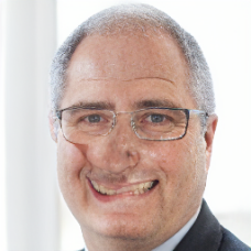
(a)

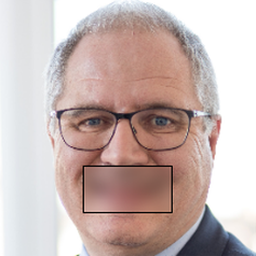
(b)

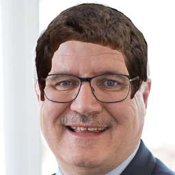
(c)

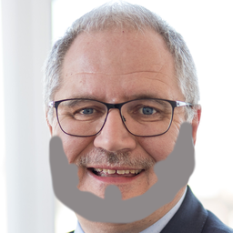
(d)

(e)

(f)

(g)

(h)

(i)

(j)

(k)

(l)

(m)

(n)

(o)

Figure 1: Using a single and straightforward training, EdiBERT can tackle a wide variety of different tasks in image editing. The first row is the input, second and third rows are different samples from EdiBERT showing realism and consistency.

Significant progress in image generation has been made in the past few years, thanks notably to Generative Adversarial Networks (GANs) (Goodfellow et al., 2014). In particular, the StyleGAN architecture (Karras et al., 2019; 2020b) yields state-of-the-art results in data-driven unconditional generative image modeling. Empirical studies have shown the usefulness of such architecture when it comes to image manipulation. For example, by following specific directions in the latent space, one can modify an image attribute such as gender, age, the pose of a person (Shen et al., 2020), or the angle (Jahanian et al., 2019). However, since the whole picture is generated from a Gaussian vector, changing some undesired elements while keeping the others frozen is difficult. To do so, edition algorithms involving optimization procedures have been proposed (Abdal et al., 2019; 2020) but with one main caveat: the results are not convincing when manipulating complex visuals (Niemeyer & Geiger, 2021) (cf. experimental section for visual results).

Independently, Van den Oord et al. (2017) propose VQVAE, a promising latent representation by training an encoder/decoder using a discrete latent space. The authors demonstrate the possibility to embed images in sequences of discrete tokens borrowing ideas from vector quantization (VQ), paving the way for the generation of images with autoregressive transformer models (Ramesh et al., 2021; Esser et al., 2021b). On top of it, we argue that one of the benefits of this representation is that each token in the sequence is mostly coding for a localized patch of pixels (see section 3.5), thus opening the possibility for an efficient localized latent edition.

Aiming to build a unified approach for image manipulation, we propose a method that leverages both the spatial property of the discrete vector-quantized representation and the use of bidirectional attention models. In particular, we train a transformer based on ideas from the language model BERT (Devlin et al., 2019), naming EdiBERT the resulting model. During training, EdiBERT tries to recover the original tokens of a perturbed sequence through a bidirectional attention schema. In computer vision, this approach has mainly been studied in the context of self-supervised learning (Bao et al., 2022; He et al., 2022). We argue that training a single model from this generic objective provides a way to handle several editing tasks. To improve the visual quality and correct the information loss due to the quantization, we propose a post-processing procedure that better recovers the pixel content outside of the edited region. With this unique training scheme and its companion sampling and post-processing algorithms, the obtained generative model can now be used in many different image manipulation tasks such as denoising, inpainting, or scribble-based editing, as shown in Figure 1.

To sum up, our contributions are the following:

• We analyze the VQ latent representations and illustrate their spatial properties, and show how to improve the reconstruction capabilities of VQGAN. This motivates the use of bidirectional transformers for image editing.

• We show how to derive two different algorithms from a single model: one for image denoising where the locations of the edits are unknown, and a second one for inpainting or image compositing where a mask specifies the area to edit.

• Finally, we show that using this generic and simple training algorithm and its companion post-processing allows us to achieve competitive results on various image manipulation tasks.

2 Related work

We start this section by introducing transformer models for image generation before motivating the VQ representation and bidirectional models for image manipulation.

2.1 Autoregressive image generation

The use of autoregressive transformer models (Vaswani et al., 2017) in computer vision has been made possible by two simultaneous research branches. First, the extensive deployment of attention mechanisms such as non-local means algorithms (Buades et al., 2005), non-local neural networks (Wang et al., 2018), and attention layers in GANs (Zhang et al., 2019; Hudson & Zitnick, 2021). Second, the development of generative models sequentially inferring pixels via autoregressive convolutional networks such as PixelCNN (Van den Oord et al., 2016a; b). Both of these works pave the way for the adoption of autoregressive transformers models in image generation (Parmar et al., 2018). The main interest of such formulation resides in a principled and tractable log-likelihood estimation of the empirical data. However, classical attention layers have a complexity scaling with the square of the sequence length, which is a bottleneck to scale to high-resolution images.

Recently, Esser et al. (2021b) were the first to apply autoregressive transformers on the discrete representation proposed by Van den Oord et al. (2017). In this framework, an encoder $E$, a decoder $D$, and a codebook/dictionary $Z$ are learned simultaneously to represent images with a single sequence of tokens. An autoregressive model is trained to generate these token sequences directly, stressing that high-capacity expressive transformers can generate realistic high-resolution images. To summarize, this framework consists of three main steps:

1. Training a VQGAN, a set of encoder/decoder/codebook $(E,D,Z)$ with perceptual and adversarial losses.

2. Training an autoregressive transformer to maximize the log-likelihood of the encoded sequences.

3. At inference, sampling a sequence with the transformer and decoding it with the decoder $D$.

This representation also allowed to improve DALL-E (Ramesh et al., 2021), a state-of-the-art text-to-image model translation.

2.2 Bidirectional attention

The main property of autoregressive models is that they only perform attention on previous tokens, making them inadequate when dealing with image manipulation (Esser et al., 2021a). Some works alleviate this bias in different ways. Yang et al. (2019) learn an autoregressive model on random permutations of the ordering. Cao et al. (2021) propose a model where missing tokens are inferred autoregressively, conditionally to the set of kept tokens. Similarly, Wan et al. (2021) use an auto-regressive procedure conditioned on the masked image, while Yu et al. (2021) use BERT training with [MASK] tokens and Gibbs sampling. If this setting is ideal for tasks with masked tokens such as inpainting, it makes it ill-posed for scribble-editing and insertion without existing paired datasets. On the opposite, our EdiBERT tackles all tasks without any need for supervision. Finally, Esser et al. (2021a) train ImageBART, a transformer that reverts a diffusion process in the discrete latent space of VQGAN. Each generated sequence is conditioned on the previous one, thus paying attention to the whole image. However, this method is computationally heavy since it requires making $N\times L$ inferences, where $N$ is the number of generated sequences and $L$ the number of tokens in the sequence. Moreover, the authors do not the limited reconstruction capabilities of VQGANs. In this paper, we argue that by performing bidirectional attention over all the tokens (perturbed or not), it is now possible to train a single model tackling many editing tasks.

2.3 Unifying image manipulation

Initially, image manipulation methods were implemented without any trainable parameters. Image completion was tackled using nearest-neighbor techniques along with a large dataset of scenes (Hays & Efros, 2007). As to image insertion, blending methods were widely used, such as the Laplacian pyramids (Burt & Adelson, 1987). In recent years, image manipulation has benefited from the advances of deep generative models. A first line of works has consisted of gathering datasets of corrupted and target images to train conditional generative models. By doing so, one can therefore learn a mapping from any corrupted image to a real one. This technique can be done using either an unpaired dataset (Zhu et al., 2017), or a paired dataset (Zhao et al., 2020). For example, Liu et al. (2021) proposes an encoder-decoder architecture for sketch-guided image inpainting. However, in all cases, a dataset with both types of images is required, therefore limiting the applicability.

To avoid this dependency, a second idea - known as GAN inversion methods - leverages pre-trained unconditional GANs. They work by projecting edited images on the manifold of real images learned by the pre-trained GAN. It can be solved either by optimization (Abdal et al., 2019; 2020; Daras et al., 2021), or with an encoder mapping from the image space to the latent space (Chai et al., 2021; Richardson et al., 2021; Tov et al., 2021). Pros of these GAN-based methods are that one benefits from outstanding properties of StyleGan, state-of-the-art in image generation. However, the main drawback of these methods is that they rely on a task-specific loss function that needs to be defined and optimized. Finally, and closer to our work is the SDEdit model proposed by Meng et al. (2022) where the authors use Langevin’s dynamics for image edition. However, the inference time of such model is still particularly slow.

3 Motivating EdiBERT for image editing

This section gives a global description of the proposed EdiBERT model. We start with notations before describing the different steps leading to the BERT-based edition.

3.1 Notations

Let $I$ be an image with a width $w$, a height $h$ and a number $c$ of channels. $I$ thus belongs to $\mathbb{R}^{h\times w\times c}$. Also, let $(E,D,Z)$ be respectively the encoder, decoder and codebook defined in VQVAE and VQGAN (Van den Oord et al., 2017; Esser et al., 2021b). The codebook consists of a finite number of tokens with fixed vectors in an embedding space. Let $Z=\{t_{1},\ldots,t_{N}\}$ with $t_{k}\in\mathbb{R}^{d}$ and $N$ being the size of the codebook.

For any given image $I$, the encoder $E$ outputs a vector $E(I)\in\mathbb{R}^{l\times d}$, which is then quantized and reshaped into a sequence $s$ of length $l$ as follows:

$$s=(\underset{z\in Z}{\text{arg min }}\|E(I)_{1}-z\|,\ldots,\underset{z\in Z}{\text{arg min }}\|E(I)_{l}-z\|))=Q_{Z}(E(I)),$$ (1)

where $Q_{Z}$ refers to the quantization operation using the codebook $Z$. Recall that, after the quantization step, one gets a sequence $s\in Z^{l}$.

Let note $\mathcal{D}$, the available image dataset. From a pre-trained encoder $E$ and codebook $Z$, one can transform the image dataset $\mathcal{D}$ into a dataset of token-sequences $\mathcal{D}_{S}$:

$$\mathcal{D}_{S}=\{Q_{Z}(E(I)),I\in\mathcal{D}\}.$$ (2)

Interestingly, when learning transformers on sequences of tokens, the practitioner is directly working with $\mathcal{D}_{S}$ and not $\mathcal{D}$.

For the rest of the paper, we consider $p_{\theta}$ a transformer model parameterized with $\Theta$. The present section aims to illustrate the chosen objective for the EdiBERT model on the dataset $\mathcal{D}_{S}$. For each position $i$ in $s$, we note $p_{\theta}^{i}(.|s)$, the modeled distribution of tokens conditionally to $s$.

3.2 Learning sequences with autoregressive models

Previous works training transformers model on $\mathcal{D}_{S}$ chose autoregressive models (Esser et al., 2021b). In this setting, for a given sequence $s=(s_{1},\ldots,s_{l})\in\mathcal{D}_{S}$ of discrete tokens, the likelihood $p_{\theta}(s)$ of the sequence $s$ is given using the following formula:

$$p_{\theta}(s)=\prod_{i=1}^{l}\ p_{\theta}^{i}(s_{i}|s_{<i}),\quad\text{with }s_{<i}=(s_{1},\ldots,s_{i-1}).$$ (3)

Since each $s_{i}\in Z$ is discrete, this decomposition is implemented thanks to a causal left-to-right attention mask and a softmax output layer. Finally, given a specified set of parameters $\Theta$, the objective of the autoregressive model is:

$$\underset{\theta\in\Theta}{\text{arg max }}\mathbb{E}_{s\in\mathcal{D}_{s}}\ \log p_{\theta}(s).$$ (4)

Limitations of the model.

If this setting is well suited for unconditional image generation, it is ill-posed for image manipulation tasks (Esser et al., 2021a). Indeed, in the case of scribble-based editing, one wants to resample tokens conditionally to the whole image. In the case of inpainting, one wants to resample tokens conditionally to a random subset of the tokens.

3.3 A unique training objective for EdiBERT.

Let us define the training objective for EdiBERT. For any sequence $s=(s_{1},...,s_{L})$, a function $\varphi$ randomly selects a subset of $k$ indices $\{\varphi_{1},...,\varphi_{k}\}$ where $\varphi_{k}<L$. At each selected position, a perturbation is applied on the token $s_{\varphi_{i}}$. We attribute a random token with probability $p$, or keep the same token with probability $1-p$. Consequently, the perturbed token $\tilde{s}_{\varphi_{i}}$ becomes:

$$\tilde{s}_{\varphi_{i}} =\mathbb{U}(Z)\quad\text{with probability }p,$$ (5)

$$\tilde{s}_{\varphi_{i}} =s_{\varphi_{i}}\quad\text{with probability }1-p,$$ (6)

where $\mathbb{U}(Z)$ refers to the uniform distribution on the space of tokens $Z$. Similarly to Bao et al. (2022), the sampling function $\varphi$ is defined with a 2D masking strategy, and the training positions are selected by drawing random 2D rectangles in the 2D patch extracted from the encoder. Note that, contrarily to Bao et al. (2022) and Devlin et al. (2019), we only use random tokens from the codebook but no [MASK] tokens. We argue this setting corresponds more to our use cases (denoising or editing), where we want to sample conditionally to an entire perturbed sequence.

Let us now call $\tilde{s}$ and $\tilde{\mathcal{D}_{s}}$, respectively the perturbed sequence and dataset:

$$\tilde{s}=(s_{1},\ldots,\tilde{s}_{\varphi_{1}},\ldots,\tilde{s}_{\varphi_{k}},\ldots,s_{L}),\quad\text{and}\quad\tilde{\mathcal{D}}=\{\tilde{s},\ s\in\mathcal{D}\}.$$ (7)

The training consists in the following objective :

$$\underset{\theta\in\Theta}{\text{arg max }}\ \mathbb{E}_{\tilde{s}\in\tilde{\mathcal{D}_{s}}}\ \frac{1}{k}\ \sum_{i=1}^{k}\log p_{\theta}^{i}(s_{\varphi_{i}}|\tilde{s}).$$ (8)

Contrary to equation 4, we note that the objective in equation 8 enforces the model to perform attention over the whole input image.

Sampling from EdiBERT:

Wang & Cho (2019) show that it is possible to generate realistic samples with a BERT model starting with a random initialization. However, compared with standard autoregressive language models, the authors stress that BERT generations are more diverse but of slightly worse quality. Building on the findings of Wang & Cho (2019), we do not aim to use BERT for pure unconditional sequence generation but rather improve an already existing sequence of tokens. In our defined EdiBERT model, for any given position $i\in s$, a token will be sampled according to the multinomial distribution $p_{\theta}^{i}(.|s)$.

3.4 On the locality of Vector Quantization encoding

In this paper, we argue that one of the main advantages of EdiBERT comes from the VQ latent space proposed by Van den Oord et al. (2017) where each image is encoded in a discrete sequence of tokens. In this section, we illustrate with simple visualizations the property of this VQGAN encoding. We explore the spatial correspondence between the position of the token in the sequence and a set of pixels for the encoded image. We aim at answering the following question: do local modifications of the image lead to local modifications of the latent representation and vice versa?

Modifying the image.

To answer this question, images are voluntarily perturbed with grey masks ($i\longrightarrow i_{m}$). Then, we encode the two images, quantize their representation using a pre-trained codebook, and plot the distance between the two latent representations: $\|Q_{Z}(E(i))-Q_{Z}(E(i_{m}))\|_{2}^{2}$. The results are shown in the first row in Figure 2. Due to the large receptive field of the encoder, tokens can be influenced by distant parts of the image: the down-sampled mask does not recover all of the modified tokens. However, tokens that are largely modified are either inside, or very close to the down-sampled mask.

Modifying the latent space.

To understand the interchange of the correspondence between tokens and pixels, we want to stress how one can easily manipulate images via the discrete latent space. We show in Figure 2 that extracting a specific area of a given source image and inserting it at a chosen location in another image is possible by replacing the corresponding tokens in the target sequence with the ones of the source. Consequently, this spatial correspondence between VQGANs latent space and image space is interesting for localized image editing tasks, i.e. tasks that require modifying only a subset of pixels without altering the other ones.

Modifying the latent space via the image space

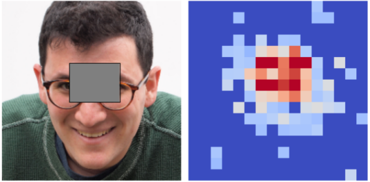
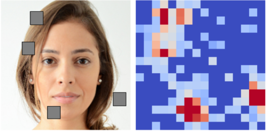
(a)

Modifying the image via the latent space

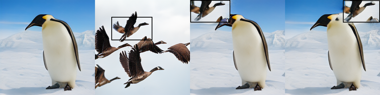
Figure 2: Each VQGAN token is strongly tied to a small spatial area in the image space. First row: perturbed images and the respective variations of tokens in the latent space. Second row: collages of images can easily be done with collages of latent representations.

3.5 On reconstruction capabilities of Vector Quantization encoding

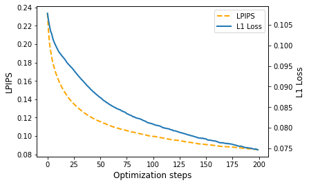
(a)

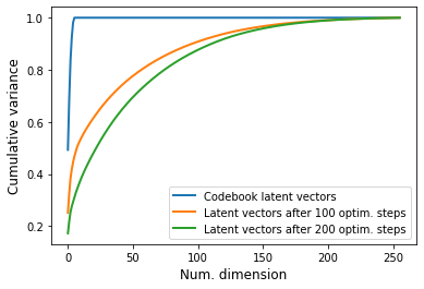
(b)

Figure 3: Analysis of reconstruction capabilities of VQGAN. On the left, we see the evolution of L1 loss and LPIPS between original and reconstructed image, when optimizing LPIPS over the latent vectors of VQGAN. On the right, we see the evolution of the number of dimension spanned by the latent vectors, before and after optimization.

A limit of the framework for the use of VQGANs for image editing resides in its reconstruction capabilities. Indeed, the vector quantization operation induces a loss of information. In this section, we highlight some limits of the reconstructions of VQGANs and propose a simple optimization scheme to improve them.

In Figure 3, we show that VQGAN struggles to properly reconstruct high-frequency details, for example complex backgrounds on FFHQ dataset (Karras et al., 2019). However, a simple optimization procedure over the latent space vectors improve the reconstruction quality of VQGANs and allows to recover fine details. The optimization consists in optimizing the LPIPS (Zhang et al., 2018) over the latent vectors: $s^{\star}=\operatorname*{arg\,min}_{s}\text{LPIPS}(D(s),I)$, where $I$ is the target image, $s$ the sequence of latent vectors and $D$ the decoder. We approximate the optimal latent vectors by gradient descent and initialize $s$ as $s=E(I)\in\mathbb{R}^{l\times d}$. Furthermore, in Figure, we show a potential explanation of the limited reconstruction capabilities of VQGAN: the latent vectors of the codebook have a very low rank. After the optimization procedure, the latent vectors span more dimensions of the embedding space.

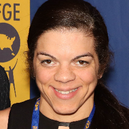
(a)

(b)

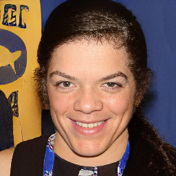
(c)

(d)

(e)

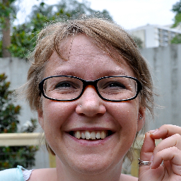
(f) Original.

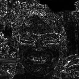
(g) Difference between original and VQGAN reconstruction.

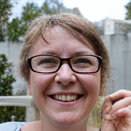
(h) VQGAN reconstruction.

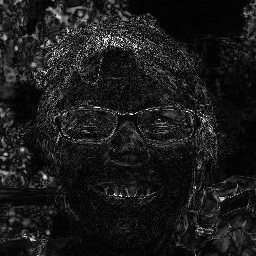
(i) Difference between original and VQGAN plus latent optimization reconstruction.

(j) VQGAN plus latent optimization reconstruction.

Figure 4: Reconstructions from VQGAN on FFHQ, before and after optimization on latent vectors.

4 Image editing with EdiBERT

In this section, we describe the use of EdiBERT to perform image editing. Specifically, we distinguish three editing tasks: image denoising, image inpainting, and image composition (including image crossover, image compositing, and scribble-based editing). On a given dataset, we tackle each different task with the same pre-trained EdiBERT model and provide below a detailed explanation of the associated sampling algorithms. We run EdiBERT on FFHQ (Karras et al., 2019) and LSUN Bedroom (Yu et al., 2015) at 256$\times$256. All metrics are reported on test-set of EdiBERT.

Baselines. For each task, we run comparisons with baselines and state-of-the-art models based on GANs inversion methods. On FFHQ, we compare to ImageStyleGAN2++ (Abdal et al., 2020) on pre-trained StyleGANs: StyleGAN2 (Karras et al., 2020b) and StyleGAN2-ADA (Karras et al., 2020a). Besides, we run the solution proposed by Chai et al. (2021) where a StyleGAN2 model is inverted using a trained encoder. Finally, we use In-Domain GAN (Zhu et al., 2020), a hybrid method combining an encoder with an optimization procedure minimizing reconstruction losses. We also compare to Co-Modulated GANs (Zhao et al., 2020), a conditional GAN for inpainting.

Metrics. We follow the work of Chai et al. (2021) and use metrics assessing both fidelity and distribution fitting. The masked L1 metric (Chai et al., 2021) measures the closeness between the generated image and the source image outside the edited areas. The density/coverage metrics (Naeem et al., 2020) are robust versions of precision/recall metrics. Intuitively, density measures fidelity while coverage measures diversity. Finally, the FID (Heusel et al., 2017) quantifies the distance between generated and target distributions. Moreover, we perform a user study on FFHQ image compositing. More details and quantitative results on LSUN Bedroom are presented in Appendix.

4.1 Localized image denoising

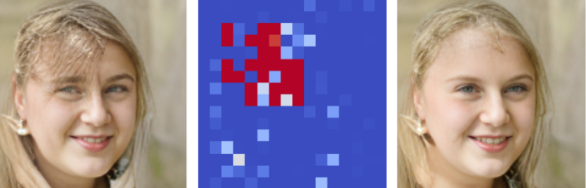
(a)

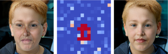
(b)

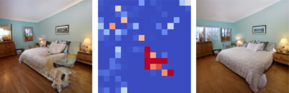
(c)

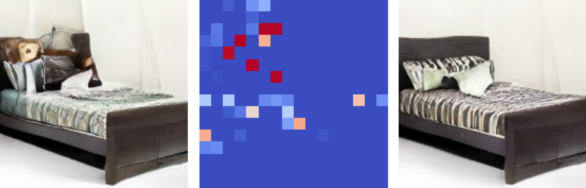
(d)

Figure 5: Image denoising with EdiBERT: the color in the different heatmaps is proportional to the negative likelihood of the token. Tokens with lower likelihood appear in red in the heatmap and have a higher probability of being sampled to be edited. We observe that conditional distributions output by EdiBERT is a good way to detect anomalies and artifacts in the image space.

Image denoising aims to improve the quality of a pre-generated image or improve a locally perturbed one. The model has to work without information on the localization of the perturbations. This means we need to find and replace the perturbed tokens with more likely ones to recover a realistic image. Thus, given a sequence $s=(s_{1},\dots,s_{L})$, we want to:

1. Detect the tokens that do not fit properly in the sequence $s$.

2. Change them for new tokens increasing the likelihood of the new sequence.

We desire a significantly more likely sequence with as few as possible token amendments. To do so, we measure the likelihood of each token $s_{i}$ based on the whole sequence $s$, aiming to compute $p(s_{i}|s)$, and replace the least-probable tokens considering them independently. That is, we propose to use the conditional probability output by the model in order to detect and sample the less likely odd tokens. Some examples of image denoising are presented in Figure 5, and we observe that EdiBERT is able to detect artifacts and replace them with more likely tokens. The full algorithm is given in the Algorithm 1.

Requires: Sequence $(s_{1},\ldots,s_{l})$, BERT model $p_{\theta}$, number of iterations $T$;

for iterations in [0,T] do

       Compute $p_{i}=\text{logit}(-p_{\theta}^{i}(s_{i}|s)),\forall i\in[1,l]$ ;

       Sample $p\sim(p_{1},\ldots,p_{l})$ (less likely position);

       Sample $t\in Z\sim p_{\theta}^{p}(\cdot|s)$ ;

       Insert sampled token: $s_{i}\leftarrow t$ ;

      

end for

$\text{Image}\leftarrow\text{Decoder}(s)$;

Result: Image

Algorithm 1 Image denoising

4.2 Image inpainting

In this setting, we have access to a masked image $i_{m}\in\mathbb{R}^{h\times w\times c}$ along with the location of the binary mask $m\in\mathbb{R}^{h\times w}$. $i_{m}$ has been obtained by masking an image $i\in\mathbb{R}^{h\times w\times c}$ as follows: $i_{m}=i\odot m$ with $\odot$ pointwise multiplication. The goal of image inpainting is to generate an image $\hat{i}$ that is both realistic (high density) and conserves non-masked parts, that is $\hat{i}\odot(1-m)=i\odot(1-m)$.

Requires: Masked (or edited) image $i_{m}$, mask $m$, Encoder E, Decoder D, BERT model $p_{\theta}$, epochs e, periodic collage c, optimization steps optim_steps;

$s\leftarrow Q(E(i_{m}))$;

$\text{latent\_mask}\leftarrow\text{get\_mask\_in\_latent\_space}(m)$;

if task is inpainting then

       $s\leftarrow s\times\text{latent\_mask}+\text{rand}\times(1-\text{latent\_mask})$;

      

end if

for e in [0,epochs] do

       for p in $\text{chosen\_order}(\text{latent\_mask})$ do

             Sample token $t\in Z\sim p_{\theta}^{p}(\cdot|s)$ ;

             Insert sampled token: $s_{p}\leftarrow t$ ;

             if p%c=0 (collage) then

                   Encode image post-collage: $s\leftarrow E(i_{m}\odot m+D(s)\odot(1-m))$;

             end if

            

       end for

      

end for

$s^{0}\leftarrow s$ ;

for i in [0, optim_steps]: do

       $L=L_{p}\big{(}(D(s)-i_{m})\odot m\big{)}+L_{p}\big{(}(D(s)-D(s^{0}))\odot(1-m)\big{)}$ ;

       $s\leftarrow s+\epsilon*\text{Adam}(\nabla_{s}L,s)$ ;

      

end for

$\text{Image}\leftarrow\text{Decoder}(s)$;

Result: Image

Algorithm 2 Image inpainting/composition

Among the different tasks in image manipulation, image inpainting stands out. Indeed, when masking a specific area of an image, one shall not consider the pixels within the mask to recover the target image. Interestingly, this is the main difference with the scribble-based or image compositing editing tasks, where, on the opposite, one must consider the modifications brought by user input. Due to these peculiarities, the image inpainting task requires specific care to reach a state-of-the-art performance; this is why we introduce five different elements to our approach. We validate these elements with visual results in Figure 6 and and an ablation study in Table 2.

1. Erasing mask influence with random tokens (randomization). To delete the information contained in the mask, all the tokens within the mask are given random values.

2. Dilating the mask in the token space (dilation). As shown in Figure 2, some tokens outside of the down-sampled mask in the latent space are also impacted by the mask. Consequently, only modifying tokens inside the down-sampled mask might not be enough and could lead to images with irregularities on the borders. As a solution, we propose to apply a dilation on the down-sampled mask and show an example of this in Figure 6. We observe that dilating the mask helps to better blend the target image’s completion since the boundaries are removed.

3. Defining a new ordering of positions (random ordering). There is no pre-defined ordering of positions in EdiBERT. One can thus look for optimal sampling of positions. We argue that by sampling positions randomly, one does not fully leverage the spatial location of the mask. Instead, we propose to use a spiral ordering that goes from the border of the mask to the inside. Figure 6 shows examples of image completion with this pre-defined ordering or random ordering. Results from Table 2 confirm the advantage of this ordering.

4. Periodic image collage (collage). To preserve fidelity to the original image, we periodically perform an image collage between the masked image and the image decoded from the current latent representation. Without this collage trick, the reconstruction can diverge too much from the input image. When performing optimization without collage, we observe border effects (see Row 3, last column in Figure 6).

5. Online optimization on latent sequence (optimization). To further improve fidelity to the masked image $i_{m}$, the final stage of our algorithm consists in an optimization procedure on the latent sequence $s\in\mathbb{R}^{h\times w\times d}$. The objective function is defined as:

   $$L=L_{p}\big{(}(D(s)-i_{m})\odot m\big{)}+L_{p}\big{(}(D(s)-D(s^{0}))\odot(1-m)\big{)}$$ (9)

   where $L_{p}$ is a perceptual loss (Zhang et al., 2018), and $s^{0}$ is the initial sequence from EdiBERT. Intuitively, the first term enforces the decoded image to get closer to the masked image $i_{m}$, while the second term is a regularization enforcing the decoded image to stay similar to the completion proposed by the transformer’s likelihood.

   If this loss function is optimized over the image space, the resulting image would be the following one: $i_{m}\odot m+D(s^{0})\odot(1-m)$. The resulting image would be non-smooth, with visible border effects. However, when optimizing over the sequence of latent vectors $s$, the decoder regularizes the optimization and avoids non-smooth borders. We illustrate in Figure 3 and Figure 6 that the optimization leads to a better-preserved source image.

Table 1: Image inpainting and compositing on FFHQ $256\times 256$. Com-GAN is a model specific for image inpainting, ID-GAN handles several editing tasks but not inpainting, while other methods handle both. We remove I2SG++ from the user study, since I2SG^†++ is the same method with a better GAN backbone, i.e. StyleGAN2-ADA (Karras et al., 2020a). Bold: $1^{st}$ rank, blue: $2^{nd}$ rank.

	Inpainting				Compositing
	Masked L1 $\downarrow$	FID $\downarrow$	Dens. $\uparrow$	Cover. $\uparrow$	Masked L1 $\downarrow$	Dens. $\uparrow$	User study $\uparrow$
I2SG++ (Abdal et al., 2020)	0.0767	23.6	0.99	0.88	0.0851	0.77	-
I2SG†++ Abdal et al. (2020)	0.0763	22.1	1.25	0.91	0.0866	1.07	8.3%
LC (Chai et al., 2021)	0.1027	27.9	1.12	0.84	0.1116	1.00	14.8%
EdiBERT $\star$	0.0290	13.8	1.16	0.98	0.0307	0.94	61.2%
Com-GAN (Zhu et al., 2020)	0.0086	10.3	1.42	1.00	-	-	-
ID-GAN (Zhu et al., 2020)	-	-	-	-	0.0570	0.75	15.7%

(a)

(b)

(c)

(d)

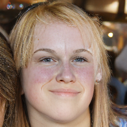
(e)

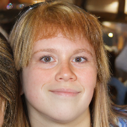
(f)

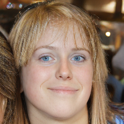
(g)

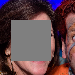
(h)

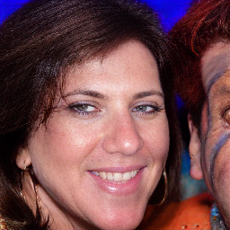
(i)

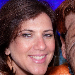
(j)

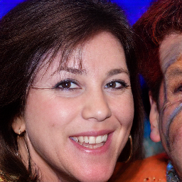
(k)

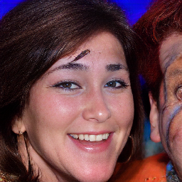
(l)

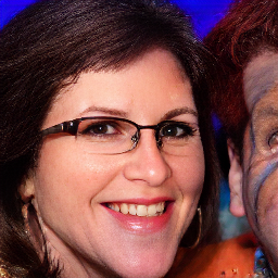
(m)

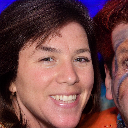
(n)

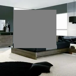
(o)

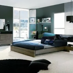
(p)

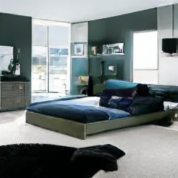
(q)

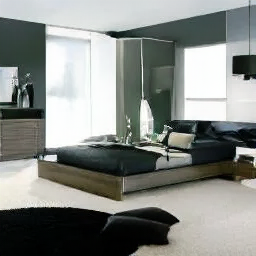
(r)

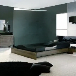
(s)

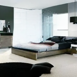
(t)

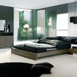
(u)

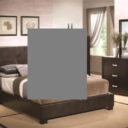
(v) Masked

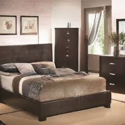
(w) EdiBERT

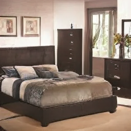
(x) (a)

(y) (b)

(z) (c)

(aa) (d)

(ab) (e)

Figure 6: Ablation study for inpainting. Components removed are (a) optimization, (b) dilation, (c) randomization, (d) collage, (e) spiraling (random order instead).

Analyzing the results:

Observing the results in Table 1, we see that the specialized method com-GAN (Zhao et al., 2020) outperforms non-specialized methods on image inpainting. This was expected since it is the only method that has been trained specifically for this task. Note that the trained model co-mod GAN cannot be used in any other image manipulation task. Compared with the non-specialized method, EdiBERT always provides better fidelity to the source image (lower Masked L1) and realism (best FID and top-2 density).

4.3 Image composition

In this setting, we have access to a non-realistically edited image $i_{e}\in\mathbb{R}^{h\times w\times c}$. The edited image $i_{e}$ is obtained by a composition between a source image $i_{s}\in\mathbb{R}^{h\times w\times c}$ and a target image $i_{t}\in\mathbb{R}^{h\times w\times c}$. The target image can be a user-drawn scribble or another real image in the case of image compositing. Besides, pixels are edited inside a binary mask $m\in\mathbb{R}^{h\times w}$, which indicates the areas modified by the user. Thus, the final edited image is computed pointwise as:

$$i_{e}=i_{s}\odot m+i_{t}\odot(1-m).$$ (10)

Image composition aims to transform an edited image $i_{e}$ to make it more realistic and faithful without limiting the changes outside the mask. We note the source image $i_{s}$ outside the mask and the edits of the target image $i_{m}$ for the inserted elements in the edition mask. Three tasks fall under this umbrella: scribble-based editing, image compositing, and image crossovers.

Results of image compositing on FFHQ are presented in Table 1. EdiBERT always has the lowest masked L1. We also present the results from a user study in Table 1. 30 users were shown 40 original and edited images, along with four results (EdiBERT and baselines). They were asked which one is preferable, accounting for both fidelity and realism. The survey shows users on average prefer EdiBERT over competing approaches. We give the detailed answers of the user study in Appendix.

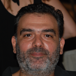
(a)

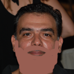
(b)

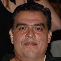
(c)

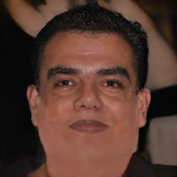
(d)

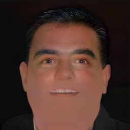
(e)

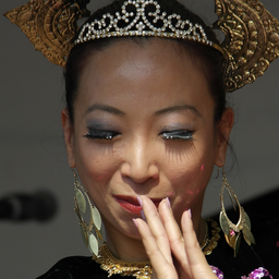
(f)

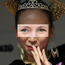
(g)

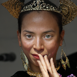
(h)

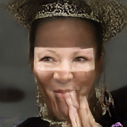
(i)

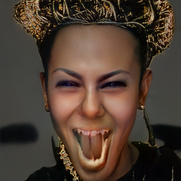
(j)

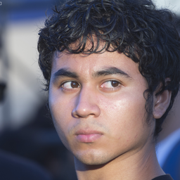
(k) Source

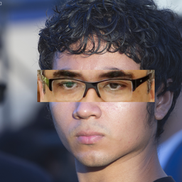
(l) Composite

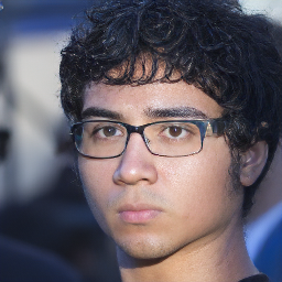
(m) EdiBERT $(\star)$

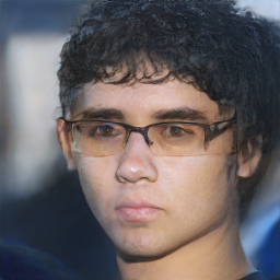
(n) ID-GAN Zhu et al. (2020)

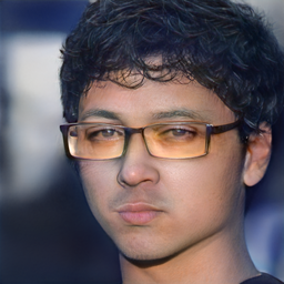
(o) I2SG^†++ Abdal et al. (2020); Karras et al. (2020a)

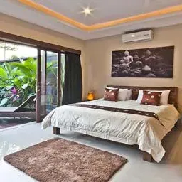
(p)

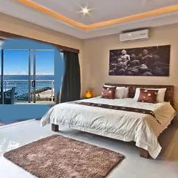
(q)

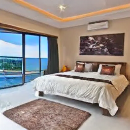
(r)

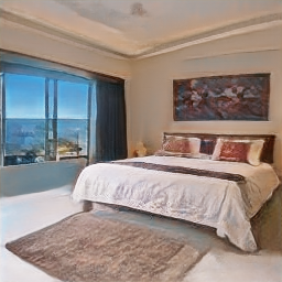
(s)

(t)

(u)

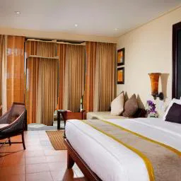
(v)

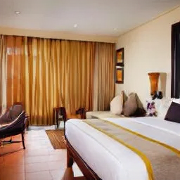
(w)

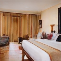
(x)

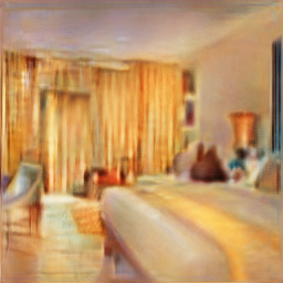
(y)

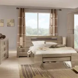
(z) Source

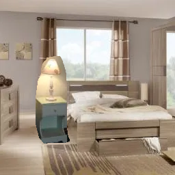
(aa) Composite

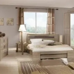
(ab) EdiBERT $(\star)$

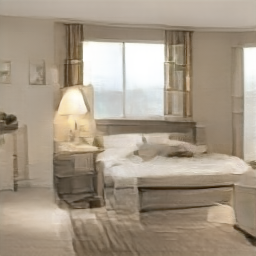
(ac) ID-GAN Zhu et al. (2020)

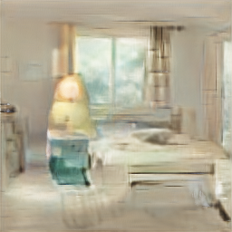
(ad) I2SG Abdal et al. (2019)

Figure 7: Scribble-based editing and image compositing: EdiBERT preserves more the connection to the source image while being able to fit the inserted object properly. This confirms the quantitative results in Table 1 where EdiBERT appears to be leading in fidelity and realism.

Table 2: Inpainting: Ablation study on the components of EdiBERT sampling algorithm. EdiBERT (1st row) shows the best tradeoff between fidelity (masked L1) and quality (FID, density/coverage). Bold: $1^{st}$ rank, blue: $2^{nd}$ rank.

Ordering	Optim-	Random-	Collage	Dilation	Masked	FID	Density	Coverage
	ization	ization			L1 $\downarrow$	$\downarrow$	$\uparrow$	$\uparrow$
Spiral	✓	✓	✓	✓	0.0201	19.4	1.14	0.96
Random	✓	✓	✓	✓	0.0206	20.7	1.13	0.95
Spiral	X	✓	✓	✓	0.0299	20.3	1.20	0.94
Spiral	✓	X	✓	✓	0.0198	20.5	1.26	0.92
Spiral	✓	✓	X	✓	0.0252	19.9	1.11	0.95
Spiral	✓	✓	✓	X	0.0197	23.3	0.96	0.91

5 Discussions

EdiBERT is a bidirectional transformers model that can tackle multiple editing tasks from one single training. One of the key elements of the proposed method is that it does not require having access to paired datasets (source, target), or unpaired image datasets. This property shows how flexible EdiBERT is and why it can be easily applied to different tasks. Overall, the proposed framework is simple and tractable: 1) train a VQGAN Esser et al. (2021b), 2) train an EdiBERT model following the objective defined in equation 8.

Interestingly, for simple applications, one can directly train EdiBERT based on the representations output by the VQGAN pre-trained on ImageNet. However, for more complex data or when dealing with multiple domains, one might have to train a specialized codebook, which requires a large auto-encoder and a lot of data. Another EdiBERT’s drawback is related to the core interest of image editing. Since the tokens are predominantly localized, EdiBERT is perfectly suited for small manipulations that only require amending a few numbers of tokens. However, some manipulations such as zooms or rotations require changing large areas of the source image. In these cases, modifying a large number of tokens might be more demanding.

Similarly to other image generative models, EdiBERT might also be used to create and propagate fake beliefs via deepfakes, as discussed in Fallis (2020).

6 Conclusion

In this paper, we demonstrated the possibility to perform several editing tasks by using the same pre-trained model. The proposed framework is simple and aims at making a step towards a unified model able to do any conceivable manipulation task on images. An exciting direction of research would be to extend the editing capabilities of EdiBERT to global transformations (e.g. zoom, rotation).

Appendix

Appendix A Implementation details

The code for the implementation of EdiBERT is available on GitHub at the following link https://github.com/EdiBERT4ImageManipulation/EdiBERT.

A pre-trained model on FFHQ is available on a linked Google Drive. Notebooks to showcase the model have also been developped.

A.1 Training hyper-parameters

We use the same architecture than Esser et al. (2021b) for both VQGAN and transformer. On LSUN Bedroom and FFHQ, we use a codebook size of 1024. For the transformer, we use a model with 32 layers of width 1024.

To train the transformer with 2D masking strategy, we generate random rectangles before flattening $Q(E(I))$. The height of rectangles is drawn uniformly from $[0.2\times h,0.5\times h]$. Similarly, the width of rectangles is drawn uniformly from $[0.2\times w,0.5\times w]$. In our experiments, since we work at resolution $256\times 256$ and follow the downsampling factor of 4 from Esser et al. (2021b), we have $h=w=256/4=16$.

Tokens outside the rectangle are used as input, to give context to the transformer, but not for back-propagation. Tokens inside the rectangle are used for back-propagation. $p_{\text{rand}}=90\%$ of tokens inside the mask are put to random tokens, while $p_{\text{same}}=1-p_{\text{rand}}=10\%$ are given their initial value. Although we did not perform a large hyper-parameter study on this parameter, we feel it is an important one. The lower $p_{\text{rand}}$, the more the learned distributions $p^{i}_{\theta}(.|s)$ will be biased towards the observed token $s_{i}$. However, setting $p_{\text{rand}}=1$ leads to a model that diverges too fast from the observed sequence.

A.2 Inference hyper-parameters

A.2.1 Image inpainting.

We set the number of epochs to 2, collage frequency to 4 per epoch, top-k sampling to 100, dilation to 1, and number of optimization steps to 200. We apply a gaussian filter on the mask for the periodic image collage.

Additionally, we use these two implementation details. 1) We use two latent masks: the latent down-sampled mask $\text{latent\_mask}_{1}$, and the dilated mask $\text{latent\_mask}_{2}$, obtained by a dilation of $\text{latent\_mask}_{1}$. The randomization is done with $\text{latent\_mask}_{1}$, such that no information from the unmasked parts of the image is erased. However, the selection of positions that are re-sampled by EdiBERT is done with $\text{latent\_mask}_{2}$. 2) At the second epoch, we randomize the token value, at the position that is being replaced. This is only done for image inpainting.

A.2.2 Image compositing.

We set the number of epochs to 2, collage frequency to 4 per epoch, top-k sampling to 100, dilation to 1, and number of optimization steps to 200. We apply a gaussian filter on the mask for the periodic image collage. Contrarily to inpainting, we do not randomize such that EdiBERT samples stay closer to the original sequence.

Appendix B Additional experimental results

We give additional comparisons on FFHQ and LSUN Bedroom, for the following tasks: image inpainting in Table 3, image crossovers in Table 4, and image composition in Table 5. All these experiments are run on the test-set of EdiBERT. Note that concurrent methods based on StyleGAN2 were trained on the full dataset, which advantages them.

Inpainting. We use 2500 images. On FFHQ, we provide results for free-form masks and rectangular masks. The height of rectangular masks is drawn uniformly from $[0.4\times h,0.6\times h]$ with $h=256$, and similarly for the width. For non-rectangular masks generations, we follow the procedure of Chai et al. (2021): we draw a binary mask at low-resolution $6\times 6$ and uspsample it to $256\times 256$ with bilinear interpolation.

The ablation study in Table 2 of main paper is performed on free-form masks. Results in Table 1 of main paper are on rectangular masks. On LSUN Bedroom, we provide results for rectangular masks.

Crossovers. We generate 2500 crossovers from random pairs of images, on both FFHQ and LSUN Bedroom.

Editing/Compositing. We create small datasets of 100 images from the test set of EdiBERT for FFHQ scribble-based editing, FFHQ compositing and LSUN Bedroom compositing. A user study on FFHQ compositing is presented in main paper with statistically significant number of votes. We also provide some metrics in 5. Because of the small size of the dataset, we only report masked L1 and density. For density, the support of the real distribution is estimated with 2500 real points, and density is averaged over the individual density of the 100 generated images.

	Masked L1 $\downarrow$	FID $\uparrow$	Density $\uparrow$	Coverage $\uparrow$
FFHQ: rect. masks
I2SG++ Abdal et al. (2020)	0.0767	23.6	0.99	0.88
I2SG†++ Abdal et al. (2020); Karras et al. (2020a)	0.0763	22.1	1.25	0.91
LC Chai et al. (2021)	0.1027	27.9	1.12	0.84
EdiBERT ($\star$)	0.0290	13.8	1.16	0.98
Co-mod. GAN Zhao et al. (2020)	0.0128	4.7	1.24	0.99
FFHQ: free-form masks
I2SG++ Abdal et al. (2020)	0.0440	22.3	0.92	0.89
I2SG†++ Abdal et al. (2020); Karras et al. (2020a)	0.0435	21.1	1.17	0.91
LC Chai et al. (2021)	0.0620	27.9	1.22	0.85
EdiBERT ($\star$)	0.0201	19.4	1.14	0.96
Com-GAN Zhao et al. (2020)	0.0086	10.3	1.42	1.00
LSUN Bedroom: rect. masks
I2SG Abdal et al. (2019)	0.1125	50.2	0.04	0.04
EdiBERT ($\star$)	0.0288	11.3	0.89	0.97

Table 3: Image inpainting.

	Masked L1 $\downarrow$	FID $\uparrow$	Density $\uparrow$	Coverage $\uparrow$
FFHQ
I2SG++ Abdal et al. (2020)	0.1141	29.4	0.97	0.78
I2SG†++ Abdal et al. (2020); Karras et al. (2020a)	0.1133	26.9	1.35	0.82
ID-GAN Zhu et al. (2020)	0.0631	23.2	0.88	0.83
LC Chai et al. (2021)	0.1491	31.9	1.17	0.77
EdiBERT ($\star$)	0.0364	19.7	1.05	0.88
LSUN Bedroom
I2SG Abdal et al. (2019)	0.1123	45.7	0.12	0.20
ID-GAN Zhu et al. (2020)	0.0682	21.4	0.35	0.57
EdiBERT ($\star$)	0.0369	12.4	0.64	0.84

Table 4: Image crossover.

	Masked L1 $\downarrow$	Density $\uparrow$
FFHQ scribble-edits
I2SG++ Abdal et al. (2020)	0.7811	0.91
I2SG†++ Abdal et al. (2020); Karras et al. (2020a)	0.0777	1.11
ID-GAN Zhu et al. (2020)	0.0461	0.79
LC Chai et al. (2021)	0.1016	1.14
EdiBERT ($\star$)	0.0281	0.96
FFHQ compositing
I2SG++ Abdal et al. (2020)	0.0851	0.77
I2SG†++ Abdal et al. (2020); Karras et al. (2020a)	0.0866	1.07
ID-GAN Zhu et al. (2020)	0.0570	0.75
LC Chai et al. (2021)	0.1116	1.00
EdiBERT ($\star$)	0.0307	0.94
LSUN Bedroom compositing
I2SG Abdal et al. (2019)	0.1285	0.25
ID-GAN Zhu et al. (2020)	0.0484	1.45
EdiBERT ($\star$)	0.0247	1.49

Table 5: Image editing.

Appendix C Baselines

We use the implementation and pre-trained models from the following repositories.

ID-GAN (Zhu et al., 2020): https://github.com/genforce/idinvert_pytorch, which has pre-trained models on FFHQ 256x256 and LSUN Bedroom 256x256.

I2SG++ and I2SG$\dagger$++(Karras et al., 2020b; a; Abdal et al., 2020):
https://github.com/NVlabs/stylegan2-ada-pytorch. We tested projections with the following pre-trained models on FFHQ: StyleGAN2 (Karras et al., 2020b) at resolution 256x256, and StyleGAN2-Ada (Karras et al., 2020a) at resolution FFHQ 1024x1024. For evaluation, we downsample the 1024x1024 generated images to 256x256.

LC (Chai et al., 2021): https://github.com/chail/latent-composition. We use the pre-trained encoder and StyleGAN2 generator, for FFHQ at resolution 1024x1024. For evaluation, we downsample the 1024x1024 generated images to 256x256.

Com-GAN Zhao et al. (2020): https://github.com/zsyzzsoft/co-mod-gan. We use the pre-trained network for image inpainting on FFHQ at resolution 512x512. We downsample the generated images to 256x256 for evaluation.

Appendix D Qualitative results on image compositon

We present more examples of image compositions, with image compositing and scribble-based editing on FFHQ in Figure 8, and image compositing on LSUN Bedroom in Figure 9.

Preservation of non-masked parts. Thanks to its VQGAN auto-encoder, EdiBERT generally better conserves areas outside the mask than GANs inversion methods. This is particularly visible for images with complex backgrounds on FFHQ (Figure 8, 5th and last rows).

Insertion of edited parts. Since EdiBERT is a probabilistic model and the tokens inside the modified area are resampled, the inserted object can be modified and mapped to a more likely object given the context. It thus generates more realistic images, but can alter the fidelity to the inserted object. For example, on row 1 of Figure 9, the green becomes lighter and the perspective of the inserted window is improved. Although it can be a downside for image compositing, note that this property is interesting for scribble-based editing, where the scribbles have to be largely transformed to get a realistic image. Contrarily, GANs inversion methods tend to conserve the inserted object too much, even if it results in a highly unrealistic generated image. We can observe this phenomenon on last row of Figure 8.

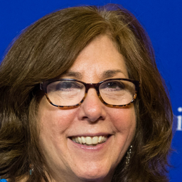
(a)

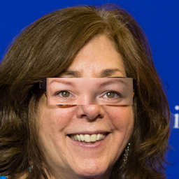
(b)

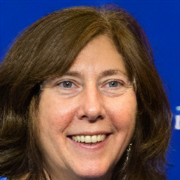
(c)

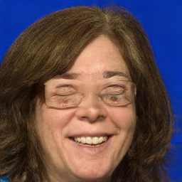
(d)

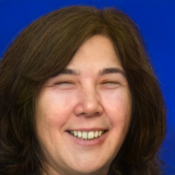
(e)

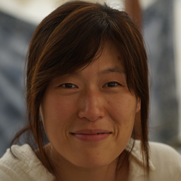
(f)

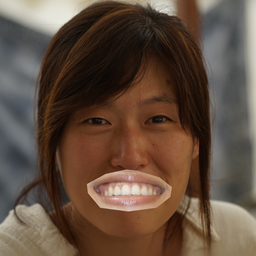
(g)

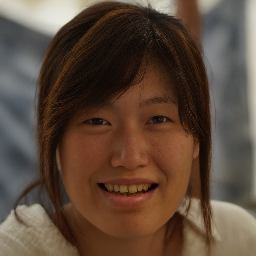
(h)

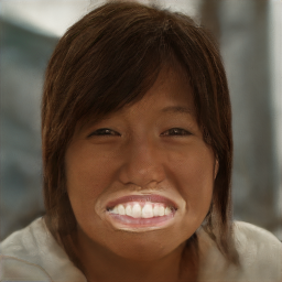
(i)

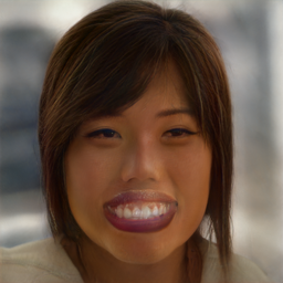
(j)

(k)

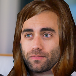
(l)

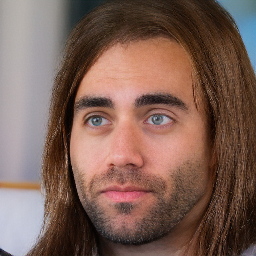
(m)

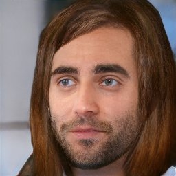
(n)

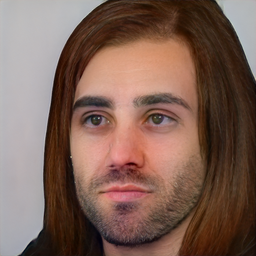
(o)

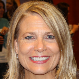
(p)

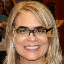
(q)

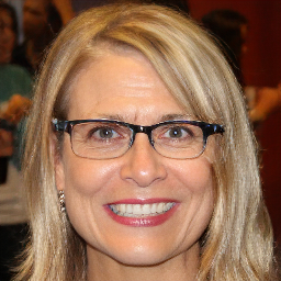
(r)

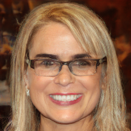
(s)

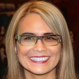
(t)

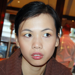
(u)

(v)

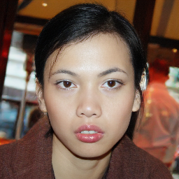
(w)

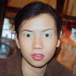
(x)

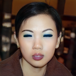
(y)

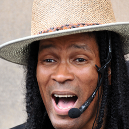
(z)

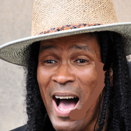
(aa)

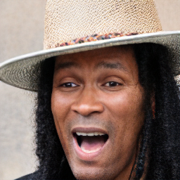
(ab)

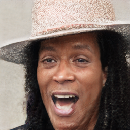
(ac)

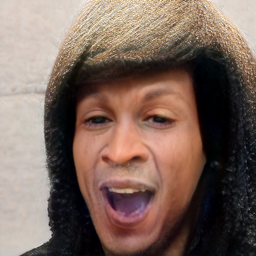
(ad)

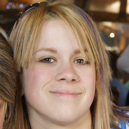
(ae) Source

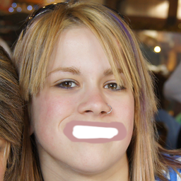
(af) Composite

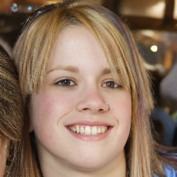
(ag) EdiBERT

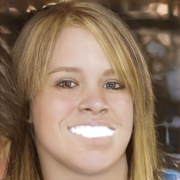
(ah) ID-GAN Zhu et al. (2020)

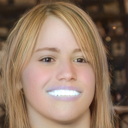
(ai) I2SG$\dagger$++ Abdal et al. (2020); Karras et al. (2020a)

Figure 8: Image compositing and scribble-based editing on FFHQ.

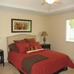
(a)

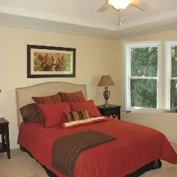
(b)

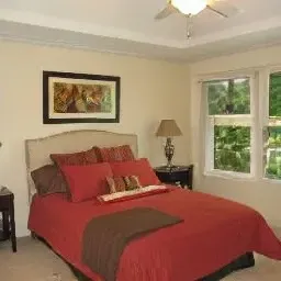
(c)

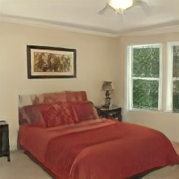
(d)

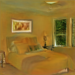
(e)

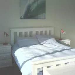
(f)

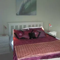
(g)

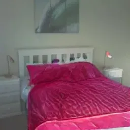
(h)

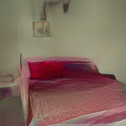
(i)

(j)

(k)

(l)

(m)

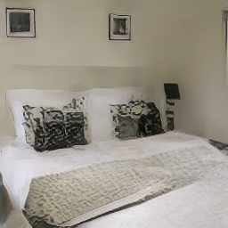
(n)

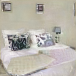
(o)

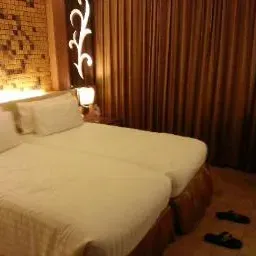
(p)

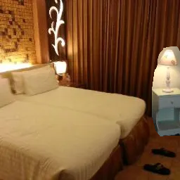
(q)

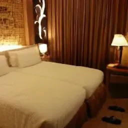
(r)

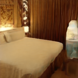
(s)

(t)

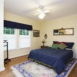
(u)

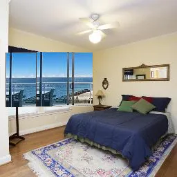
(v)

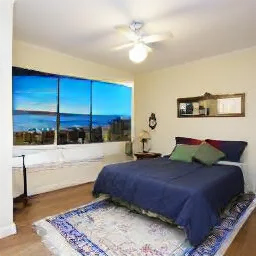
(w)

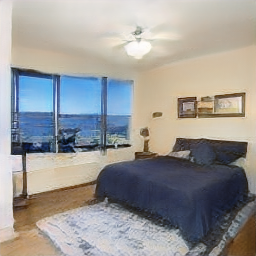
(x)

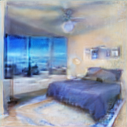
(y)

(z) Source

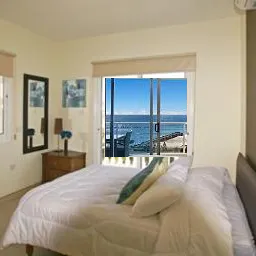
(aa) Composite

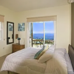
(ab) EdiBERT

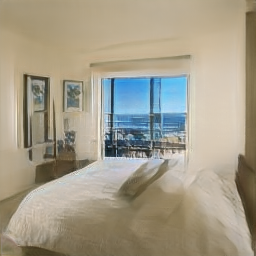
(ac) ID-GAN Zhu et al. (2020)

(ad) I2SG Abdal et al. (2019)

Figure 9: Image compositing on LSUN Bedroom.

Appendix E Survey on FFHQ image compositing

The survey was presented as a Google Form with 40 questions. For each question, the user was shown 6 images: Source, Composite, EdiBERT, ID-GAN Zhu et al. (2020), I2SG$\dagger$++ Abdal et al. (2019); Karras et al. (2020a), LC Chai et al. (2021). The different generated images were referred as Algorithm 1, …, Algorithm 4. The user was asked to vote for its preferred generated image, by taking into account realism and fidelity criterions. The user had no time limit for the poll. 30 users answered our poll. We provide the detailed answers for each image in Table 6.

	EdiBERT	ID-GAN Zhu et al. (2020)	LC Chai et al. (2021)	I2SG$\dagger$++ Abdal et al. (2019); Karras et al. (2020a)
	17	5	7	1
	15	1	8	6
	22	4	1	3
	19	4	5	2
	22	0	4	4
	6	7	8	9
	21	1	5	3
	23	1	4	2
	20	5	5	0
	11	13	6	0
	27	0	3	0
	12	3	3	12
	16	4	6	4
	25	2	1	2
	18	8	1	3
	8	13	9	0
	26	0	4	0
	7	0	21	2
	14	9	1	6
	27	0	1	2
	11	19	0	0
	14	9	4	3
	16	14	0	0
	21	1	3	5
	8	2	18	2
	19	3	3	5
	22	7	0	1
	23	2	1	4
	18	0	2	10
	27	2	1	0
	22	2	1	5
	24	0	5	1
	3	25	2	0
	28	0	2	0
	24	0	6	0
	27	0	3	0
	27	1	2	0
	22	7	1	0
	9	15	6	0
	14	0	14	2
Total	735 (61.25%)	189 (15.75%)	177 (14.75%)	99 (0.0825%)

Table 6: Detailed results of the user study. Each line corresponds to an image, with the associated number of votes per method.

References

- Abdal et al. (2019) Rameen Abdal, Yipeng Qin, and Peter Wonka. Image2stylegan: How to embed images into the stylegan latent space? In Proceedings of the IEEE/CVF International Conference on Computer Vision, pp. 4432–4441, 2019.
- Abdal et al. (2020) Rameen Abdal, Yipeng Qin, and Peter Wonka. Image2stylegan++: How to edit the embedded images? In Proceedings of the IEEE/CVF Conference on Computer Vision and Pattern Recognition, pp. 8296–8305, 2020.
- Bao et al. (2022) Hangbo Bao, Li Dong, Songhao Piao, and Furu Wei. BEit: BERT pre-training of image transformers. In International Conference on Learning Representations, 2022.
- Buades et al. (2005) Antoni Buades, Bartomeu Coll, and J-M Morel. A non-local algorithm for image denoising. In 2005 IEEE Computer Society Conference on Computer Vision and Pattern Recognition (CVPR’05), volume 2, pp. 60–65. IEEE, 2005.
- Burt & Adelson (1987) Peter J Burt and Edward H Adelson. The laplacian pyramid as a compact image code. In Readings in computer vision, pp. 671–679. Elsevier, 1987.
- Cao et al. (2021) Chenjie Cao, Yuxin Hong, Xiang Li, Chengrong Wang, Chengming Xu, Yanwei Fu, and Xiangyang Xue. The image local autoregressive transformer. In Advances in Neural Information Processing Systems, 2021.
- Chai et al. (2021) Lucy Chai, Jonas Wulff, and Phillip Isola. Using latent space regression to analyze and leverage compositionality in gans. arXiv:2103.10426, 2021.
- Daras et al. (2021) Giannis Daras, Joseph Dean, Ajil Jalal, and Alex Dimakis. Intermediate layer optimization for inverse problems using deep generative models. In Marina Meila and Tong Zhang (eds.), Proceedings of the 38th International Conference on Machine Learning, volume 139 of Proceedings of Machine Learning Research, pp. 2421–2432. PMLR, 18–24 Jul 2021.
- Devlin et al. (2019) Jacob Devlin, Ming-Wei Chang, Kenton Lee, and Kristina Toutanova. Bert: Pre-training of deep bidirectional transformers for language understanding. In Conference of the North American Chapter of the Association for Computational Linguistics: Human Language Technologies, Volume 1 (Long and Short Papers), pp. 4171–4186, 2019.
- Esser et al. (2021a) Patrick Esser, Robin Rombach, Andreas Blattmann, and Bjorn Ommer. Imagebart: Bidirectional context with multinomial diffusion for autoregressive image synthesis. Advances in Neural Information Processing Systems, 34, 2021a.
- Esser et al. (2021b) Patrick Esser, Robin Rombach, and Bjorn Ommer. Taming transformers for high-resolution image synthesis. In Proceedings of the IEEE/CVF Conference on Computer Vision and Pattern Recognition, pp. 12873–12883, 2021b.
- Fallis (2020) Don Fallis. The epistemic threat of deepfakes. Philosophy & Technology, pp. 1–21, 2020.
- Goodfellow et al. (2014) Ian Goodfellow, Jean Pouget-Abadie, Mehdi Mirza, Bing Xu, David Warde-Farley, Sherjil Ozair, Aaron Courville, and Yoshua Bengio. Generative adversarial nets. Advances in neural information processing systems, 27, 2014.
- Hays & Efros (2007) James Hays and Alexei A Efros. Scene completion using millions of photographs. ACM Transactions on Graphics (ToG), 26(3), 2007.
- He et al. (2022) Kaiming He, Xinlei Chen, Saining Xie, Yanghao Li, Piotr Dollár, and Ross Girshick. Masked autoencoders are scalable vision learners. In Proceedings of the IEEE/CVF Conference on Computer Vision and Pattern Recognition, pp. 16000–16009, 2022.
- Heusel et al. (2017) M. Heusel, H. Ramsauer, T. Unterthiner, B. Nessler, and S. Hochreiter. Gans trained by a two time-scale update rule converge to a local nash equilibrium. In Advances in Neural Information Processing Systems, pp. 6626–6637, 2017.
- Hudson & Zitnick (2021) Drew A Hudson and Larry Zitnick. Generative adversarial transformers. In Marina Meila and Tong Zhang (eds.), Proceedings of the 38th International Conference on Machine Learning, volume 139 of Proceedings of Machine Learning Research, pp. 4487–4499. PMLR, 18–24 Jul 2021. URL https://proceedings.mlr.press/v139/hudson21a.html.
- Jahanian et al. (2019) Ali Jahanian, Lucy Chai, and Phillip Isola. On the" steerability" of generative adversarial networks. In International Conference on Learning Representations, 2019.
- Karras et al. (2019) T. Karras, S. Laine, and T. Aila. A style-based generator architecture for generative adversarial networks. In Proceedings of the IEEE Conference on Computer Vision and Pattern Recognition, pp. 4401–4410, 2019.
- Karras et al. (2020a) Tero Karras, Miika Aittala, Janne Hellsten, Samuli Laine, Jaakko Lehtinen, and Timo Aila. Training generative adversarial networks with limited data. In H. Larochelle, M. Ranzato, R. Hadsell, M. F. Balcan, and H. Lin (eds.), Advances in Neural Information Processing Systems, volume 33, pp. 12104–12114, 2020a.
- Karras et al. (2020b) Tero Karras, Samuli Laine, Miika Aittala, Janne Hellsten, Jaakko Lehtinen, and Timo Aila. Analyzing and improving the image quality of stylegan. In Proceedings of the IEEE/CVF Conference on Computer Vision and Pattern Recognition, pp. 8110–8119, 2020b.
- Liu et al. (2021) Hongyu Liu, Ziyu Wan, Wei Huang, Yibing Song, Xintong Han, Jing Liao, Bin Jiang, and Wei Liu. Deflocnet: Deep image editing via flexible low-level controls. In Proceedings of the IEEE/CVF Conference on Computer Vision and Pattern Recognition, pp. 10765–10774, 2021.
- Meng et al. (2022) Chenlin Meng, Yutong He, Yang Song, Jiaming Song, Jiajun Wu, Jun-Yan Zhu, and Stefano Ermon. SDEdit: Guided image synthesis and editing with stochastic differential equations. In International Conference on Learning Representations, 2022.
- Naeem et al. (2020) Muhammad Ferjad Naeem, Seong Joon Oh, Youngjung Uh, Yunjey Choi, and Jaejun Yoo. Reliable fidelity and diversity metrics for generative models. In International Conference on Machine Learning, pp. 7176–7185. PMLR, 2020.
- Niemeyer & Geiger (2021) Michael Niemeyer and Andreas Geiger. Giraffe: Representing scenes as compositional generative neural feature fields. In Proceedings of the IEEE/CVF Conference on Computer Vision and Pattern Recognition, pp. 11453–11464, 2021.
- Parmar et al. (2018) Niki Parmar, Ashish Vaswani, Jakob Uszkoreit, Lukasz Kaiser, Noam Shazeer, Alexander Ku, and Dustin Tran. Image transformer. In International Conference on Machine Learning, pp. 4055–4064. PMLR, 2018.
- Ramesh et al. (2021) Aditya Ramesh, Mikhail Pavlov, Gabriel Goh, Scott Gray, Chelsea Voss, Alec Radford, Mark Chen, and Ilya Sutskever. Zero-shot text-to-image generation. arXiv:2102.12092, 2021.
- Richardson et al. (2021) Elad Richardson, Yuval Alaluf, Or Patashnik, Yotam Nitzan, Yaniv Azar, Stav Shapiro, and Daniel Cohen-Or. Encoding in style: a stylegan encoder for image-to-image translation. In Proceedings of the IEEE/CVF Conference on Computer Vision and Pattern Recognition, pp. 2287–2296, 2021.
- Shen et al. (2020) Yujun Shen, Jinjin Gu, Xiaoou Tang, and Bolei Zhou. Interpreting the latent space of gans for semantic face editing. In Proceedings of the IEEE/CVF Conference on Computer Vision and Pattern Recognition, pp. 9243–9252, 2020.
- Tov et al. (2021) Omer Tov, Yuval Alaluf, Yotam Nitzan, Or Patashnik, and Daniel Cohen-Or. Designing an encoder for stylegan image manipulation. ACM Transactions on Graphics (TOG), 40(4):1–14, 2021.
- Van den Oord et al. (2016a) Aaron Van den Oord, Nal Kalchbrenner, and Koray Kavukcuoglu. Pixel recurrent neural networks. In International Conference on Machine Learning, pp. 1747–1756. PMLR, 2016a.
- Van den Oord et al. (2016b) Aaron Van den Oord, Nal Kalchbrenner, Oriol Vinyals, Lasse Espeholt, Alex Graves, and Koray Kavukcuoglu. Conditional image generation with pixelcnn decoders. In Proceedings of the 30th International Conference on Neural Information Processing Systems, pp. 4797–4805, 2016b.
- Van den Oord et al. (2017) Aaron Van den Oord, Oriol Vinyals, and Koray Kavukcuoglu. Neural discrete representation learning. In Proceedings of the 31st International Conference on Neural Information Processing Systems, pp. 6309–6318, 2017.
- Vaswani et al. (2017) Ashish Vaswani, Noam Shazeer, Niki Parmar, Jakob Uszkoreit, Llion Jones, Aidan N Gomez, Łukasz Kaiser, and Illia Polosukhin. Attention is all you need. In Advances in neural information processing systems, pp. 5998–6008, 2017.
- Wan et al. (2021) Ziyu Wan, Jingbo Zhang, Dongdong Chen, and Jing Liao. High-fidelity pluralistic image completion with transformers. In Proceedings of the IEEE/CVF International Conference on Computer Vision, pp. 4692–4701, 2021.
- Wang & Cho (2019) Alex Wang and Kyunghyun Cho. Bert has a mouth, and it must speak: Bert as a markov random field language model. arXiv:1902.04094, 2019.
- Wang et al. (2018) Xiaolong Wang, Ross Girshick, Abhinav Gupta, and Kaiming He. Non-local neural networks. In Proceedings of the IEEE conference on computer vision and pattern recognition, pp. 7794–7803, 2018.
- Yang et al. (2019) Zhilin Yang, Zihang Dai, Yiming Yang, Jaime Carbonell, Russ R Salakhutdinov, and Quoc V Le. Xlnet: Generalized autoregressive pretraining for language understanding. Advances in neural information processing systems, 32, 2019.
- Yu et al. (2015) Fisher Yu, Yinda Zhang, Shuran Song, Ari Seff, and Jianxiong Xiao. Lsun: Construction of a large-scale image dataset using deep learning with humans in the loop. arXiv:1506.03365, 2015.
- Yu et al. (2021) Yingchen Yu, Fangneng Zhan, Rongliang Wu, Jianxiong Pan, Kaiwen Cui, Shijian Lu, Feiying Ma, Xuansong Xie, and Chunyan Miao. Diverse image inpainting with bidirectional and autoregressive transformers. In Proceedings of the 29th ACM International Conference on Multimedia, pp. 69–78, 2021.
- Zhang et al. (2019) Han Zhang, Ian Goodfellow, Dimitris Metaxas, and Augustus Odena. Self-attention generative adversarial networks. In Proceedings of the 36th International Conference on Machine Learning, volume 97 of Proceedings of Machine Learning Research, pp. 7354–7363, 2019.
- Zhang et al. (2018) Richard Zhang, Phillip Isola, Alexei A Efros, Eli Shechtman, and Oliver Wang. The unreasonable effectiveness of deep features as a perceptual metric. In Proceedings of the IEEE conference on computer vision and pattern recognition, pp. 586–595, 2018.
- Zhao et al. (2020) Shengyu Zhao, Jonathan Cui, Yilun Sheng, Yue Dong, Xiao Liang, I Eric, Chao Chang, and Yan Xu. Large scale image completion via co-modulated generative adversarial networks. In International Conference on Learning Representations, 2020.
- Zhu et al. (2020) Jiapeng Zhu, Yujun Shen, Deli Zhao, and Bolei Zhou. In-domain gan inversion for real image editing. In European conference on computer vision, pp. 592–608. Springer, 2020.
- Zhu et al. (2017) Jun-Yan Zhu, Taesung Park, Phillip Isola, and Alexei A Efros. Unpaired image-to-image translation using cycle-consistent adversarial networks. In Proceedings of the IEEE international conference on computer vision, pp. 2223–2232, 2017.