Subterahertz Radius and Limb Brightening of the Sun Derived from SST and ALMA

Abstract

Measurements of the radius and limb brightening of the Sun provide important information about the solar atmosphere structure and temperature. The solar radius increases as the observation at radio frequency decreases, indicating that each emission originates higher in the atmosphere. Thus, different layers of the solar atmosphere can be probed by observing at multiple wavelengths. In this work, we determined the average radius and limb brightening at 100, 212, 230, and 405 GHz, using data from the Solar Submillimeter Telescope and ALMA’s single-dish observations. For the first time, limb brightening values for frequencies of 212 and 405 GHz were estimated. At sub-THz frequencies, the observed limb brightening may affect the solar radius measurements. We use two different and well known approaches to determine the radius: the half-power method and the inflection-point method. We investigate how the antenna beam size and the limb brightening level, $L\!B$, can affect the radius measurements using both methods. Our results showed that the inflection-point method is the least affected by these parameters, and should thus be used for solar radius estimates at radio wavelengths. The measured average radii are $$$\pm$$$ (100 GHz), $$$\pm$$$ (212 GHz), $$$\pm$$$ (230 GHz), and $$$\pm$$$ (405 GHz). Finally, we used forward modeling to estimate the ranges of $L\!B$ of the solar disk resulting in 5%-19% (100 GHz), 2%-12% (212 GHz), 6%-18% (230 GHz), and 3%-17% (405 GHz). Both radius and limb brightening estimates agree with previous measurements reported in the literature.

1 Introduction

Investigated and measured for over 2 millenia, the optical radius of the Sun is a fundamental parameter. Records of measurements by Greek astronomers date back to the 3^rd century B.C., when they determined the apparent mean solar radius between $810\mathrm{″}$ and $988\mathrm{″}$ (Rozelot et al., 2018). Despite their ingenuity, the measurements were highly uncertain, and it took centuries for this matter to be revisited, regaining attention only in the 17^th century and being often studied from then on. Gilliland (1981) and Vaquero et al. (2016), for instance, compiled data from the 18^th until the 21^st century obtained from different observatories and authors. With measurements of the solar radius, other features and aspects were discovered, such as the variation of the solar apparent size throughout the year due to Earth’s orbital eccentricity. Also, measurements of small variations in the solar optical radius are a critical probe of the Sun’s interior stratification (Emilio et al., 2000).

Due to technological limitations, until some decades ago only optical measurements were available. Since then, measurements at radio frequencies began to take place (Coates, 1958). By observing the Sun at different radio wavelengths, the radius measurements present an exponential trend, as showed by Menezes et al. (2021), decreasing with frequency. Therefore at a specific wavelength, the difference of the measured radius from the optical radius can be understood as the height above the photosphere where most of the emission is being created in the limb regions. Moreover, the study of the solar radius at different wavelengths, derived from eclipse and direct observations, enables probing the solar atmosphere throughout the solar activity cycle (Swanson, 1973; Costa et al., 1999; Menezes & Valio, 2017; Selhorst et al., 2019b).

The canonical value at optical wavelengths of the mean apparent solar radius is $959.63\mathrm{″}$ (Auwers, 1891). There are different techniques to measure the solar radius, such as helioseismic methods from the $f$-modes (Antia, 1998; Kosovichev & Rozelot, 2018), determination from total solar eclipse observations (Kubo, 1993; Kilcik et al., 2009), and from direct observations (Emilio et al., 2000). Brown & Christensen-Dalsgaard (1998) used the Solar Diameter Monitor instrument (Brown et al., 1982) and defined the solar limb using the finite Fourier transform definition (FFTD) to measure the optical radius.

At radio wavelengths, the radius can be measured by the inflection-point method (Alissandrakis et al., 2017; Menezes et al., 2021), and by the half-power method (Costa et al., 1999; Selhorst et al., 2011; Menezes & Valio, 2017). The measurement of the solar radius by any of theses two methods is considerably affected by the presence of limb brightening in the solar disk. Mainly, because the center-to-limb average distance of the solar disk is used to define the radius, and the limb coordinates determination is affected by the limb brightening level, $L\!B$, of the brightness temperature, $T\!_{B}$, profile. In this work we define $L\!B=T_{B}/T_{qS}-1$, i.e., the percentage above the quiet Sun temperature, $T\!_{qS}$.

The solar limb brightening (or darkening) is a property that provides important information about the temperature gradient of the solar atmosphere. Solar atmospheric models predict a positive temperature gradient above the photospheric minimum temperature (e.g., Vernazza et al., 1981; Fontenla et al., 1993; Selhorst et al., 2005). This translates to an increase in the $T\!_{B}$ from submillimetric to centimetric wavelengths, because the emission at these wavelengths are formed above the minimum temperature region, where the temperature gradient is positive.

Based on maps obtained since 1992 by the Nobeyama Radioheliograph at 17 GHz (NoRH, Nakajima et al., 1994), Shibasaki (1998) reported regions near the solar poles with $T\!_{B}$ values up to 40% above the quiet-Sun value, in contrast with equatorial limb regions which presented only a 10% increase. The limb brightening of the solar disk has been registered in observations at several bands of the electromagnetic spectrum: at 1.3 mm (Withbroe, 1970), UV (Horne et al., 1981), between 350 $\mu$m and 1 m (Lindsey & Hudson, 1976), at 17 GHz (Selhorst et al., 2003; Shibasaki, 1998), 860 GHz (Lindsey et al., 1981), and at 100 and 230 GHz (Selhorst et al., 2019b). According to Selhorst et al. (2003), at 17 GHz the average intensity of the poles was found to be approximately 13% and 14% above the quiet-Sun level, $T\!_{qS}$, in the North and South poles, respectively. At 100 GHz, Selhorst et al. (2019b) found that the average brightness above $T\!_{qS}$ was 6.1% $\pm$ 2.8% at the North pole and 5.1% $\pm$ 2.7% at the South pole; whereas at 230 GHz, the average values were 9% $\pm$ 5% and 9% $\pm$ 4%, respectively for the South and North poles.

At sub-THz frequencies – i.e., millimeter and submillimeter wavelengths – there is a lack of measurements of the radius, as well as other parameters of the solar atmosphere. Since observation at distinct wavelengths probe different layers of the solar atmosphere, the study of the solar radius and limb brightening provides important information about the solar atmosphere structure and temperature.

This work is a follow-up of Menezes et al. (2021), in which we measured the average equatorial and polar radius at 212 and 405 GHz (using all receivers of the Submillimeter Solar Telescope) from 2007 to 2019, and at 100 and 230 GHz from 2015 to 2018. Also it was focused on the relation between solar radius time series and solar activity. Here, we focus on the mean radius and limb of the full sub-THz solar disk. We measure the mean solar radii at 100, 212 (receiver #3), 230, and 405 GHz (receiver #5) during a 4-year, period from 2015 to 2018. Two methods to calculate the radius at radio frequencies are considered and compared: the inflection-point and the half-power (defined in Section 3). Forward modeling is used to investigate the effect that parameters such as antenna beam size (HPBW) and $L\!B$ have on the solar radius measurements for both methods. Finally, we estimate the limb brightening above quiet-Sun values for these sub-THz frequencies.

2 Observations

2.1 Radio Telescopes

For the determination of the solar radii and the estimate of the limb brightening we used data provided by solar observations of the Atacama Large Millimeter/submillimeter Array (ALMA; Wootten & Thompson, 2009) at 100 and 230 GHz, and by the Solar Submillimeter-wave Telescope (SST; Kaufmann et al., 2008) at 212 and 405 GHz. ALMA is an international radio interferometer located in the Atacama Desert of northern Chile at 5000 m elevation.

SST is a radio telescope located at CASLEO Observatory in Argentina, at 2552 m elevation. The telescope is composed of six receivers, being two radiometers at 405 GHz and four at 212 GHz, with an absolute pointing accuracy of about $10\mathrm{″}$. Since structural antenna deformations change the expected size and form of the beams (Valle Silva et al., 2021), in this study we only use receivers #3 (212 GHz) and #5 (405 GHz), which beams have less deformation compared to the other ones.

2.2 Solar maps

SST solar maps are obtained from parallel or radial raster scans of the Sun covering an area of about a $$$\times$$$ in the sky with a tracking speed in the range of $0.1\mathrm{°}$ and $0.2\mathrm{°}$ per second. A few solar maps are reconstructed from radial and RA-dec raster scans, whereas the vast majority of the solar maps are reconstructed from azimuth-elevation scans with a $2\mathrm{\prime }$ separation between scans obtained (Giménez de Castro et al., 2020; Valle Silva et al., 2021; Menezes et al., 2021). For a typical integration time of 0.04s, the rectangular pixels are $$$\times$$$ in size. The SST maps were then interpolated to square maps of $600\times 600$ pixels.

During the years of 2015 to 2018, a total of 2148 maps at 212 GHz and 1256 maps at 405 GHz were selected for this study (the selection criteria are described in Section 3). Examples of the SST azimuth-elevation interpolated maps at 212 GHz (top left panel) and 405 GHz (top right panel) are shown in Fig. 1, where the color scale represents $T\!_{B}$.

From ALMA, we use fast-scan single-dish maps obtained in Band 3 (84–116 GHz, hereafter, 100 GHz) and in Band 6 (211–275 GHz, hereafter, 230 GHz), described by White et al. (2017). We analyzed 125 maps at 100 GHz and 71 at 230 GHz (196 in total). These maps were made during four solar observation campaigns from 2015 to 2018 by ALMA’s 12-meter single-dish. The images were extracted from FITS files provided by ALMA’s science verification page and ALMA science archive page. Examples of ALMA maps obtained at 100 GHz (bottom left panel) and 230 GHz (bottom right panel) are shown in Fig. 1, where the color scale represents the brightness temperature, $T\!_{B}$.

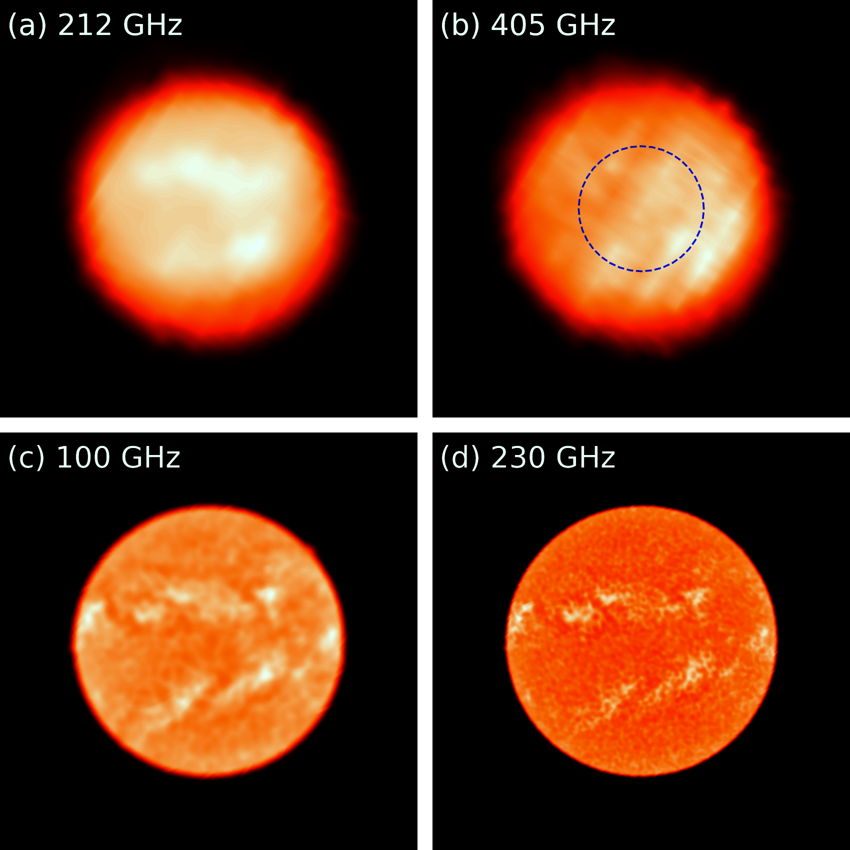
Figure 1: Solar maps obtained on 2015-12-17 from SST (upper panels) and ALMA (lower panels) at (a) 212 GHz, (b) 405 GHz, (c) 100 GHz, and (d) 230 GHz. The blue circle (b) with a radius of $7.5\mathrm{\prime }$ constrains the area used to define $T\!_{qS}$.

2.3 Antenna beam

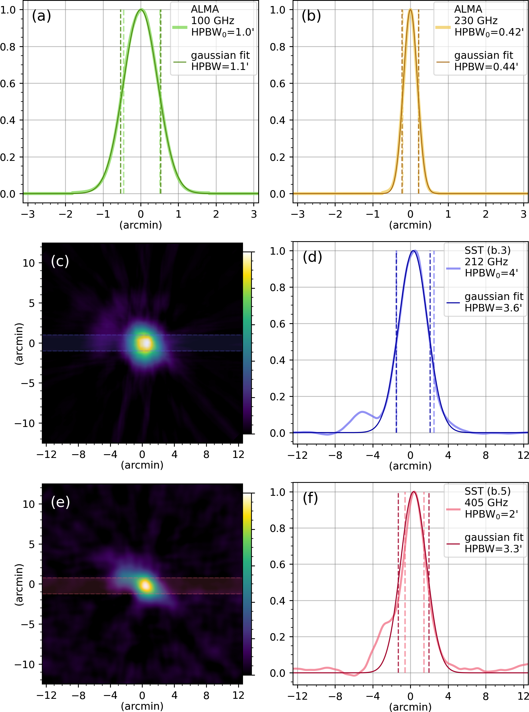
Figure 2: Reconstructed 1-D beam profiles from ALMA’s single-dish at 100 (a) and 230 GHz (b), and from SST’s antenna at 212 (d) and 405 GHz (f). Thicker lighter curves represent reconstructed beam profiles (HPBW₀ ), and thinner darker curves represent Gaussian fits of the 1-D profiles. Panels c (beam #3, 212 GHz) and e (beam #5, 405 GHz) show 2-D SST beam profiles interpolated in 600$\times$600 pixels, $2.4\mathrm{″}$/pixel.

One of the most important features that influence the measurement of the radius and limb brightening is the antenna beam width. ALMA’s single-dish nominal half-power beam widths, HPBW₀, are $58\mathrm{″}$ at 100 GHz and $25\mathrm{″}$ at 230 GHz. SST’s antenna nominal HPBW₀ are $4\mathrm{\prime }$ and $2\mathrm{\prime }$ at 212 and 405 GHz, respectively. However, to compare the radius measurement methods and to perform solar scan simulations, the true antenna beam profiles are necessary.

ALMA beams were reconstructed using the derivatives of the solar equator $T\!_{B}$ profiles extracted from all the solar maps, such as those of Fig. 1. Limb brightening/darkening affects the derivative, however due to the number of maps (the derivatives are superimposed), and to the high spatial resolution of ALMA single-dish, $T\!_{B}$ profiles derivatives are good approximations for the beam. Differences between this approximation and a 2D Gaussian beam model reconstructed with a point source, are negligible in this study. The average of all derivatives is the 1-D reconstructed beam, which are shown in panels a and b of Fig. 2.

The 2-D SST beam profiles were determined using a solar scans’ tomography procedure described in Costa et al. (2002), and are shown in panels c (212 GHz) and e (405 GHz) of Fig. 2. The SST 1-D beam profiles were obtained by averaging a band of $2\mathrm{\prime }$ width centered on the 2-D profile peak, and are shown in panels d and f of Fig. 2 for 212 and 405 GHz, respectively. As the SST beam is asymmetric, 1-D convolutions may differ from 2-D convolutions. To analyze that, we performed 2-D convolutions of SST beams and synthetic $T\!_{B}$ profiles, with $L\!B$ of 10%, 20%, 30% and 40%, and R_synth of $960\mathrm{″}$ and $970\mathrm{″}$. The radii and $L\!B$ derived from the 2-D convolutions are very close to the 1-D convolutions (differences less than $0.5\mathrm{″}$ in radius and less than 1% in $L\!B$). Therefore, we use the 1-D beam for the analysis.

These four 1-D beams at 100, 212, 230, and 415 GHz are shown in panels (a), (b), (d), and (f) of Fig. 2, respectively, were then fit by a Gaussian function to estimate the real HPBW. These fits, also shown in each panel of Fig. 2, yield values of $1.1\mathrm{\prime }$, $3.6\mathrm{\prime }$, $0.44\mathrm{\prime }$ and $3.3\mathrm{\prime }$ for 100, 212, 230, and 405 GHz, respectively. Here we use the HPBW obtained from the Gaussian fits as the reference HPBW.

3 Radius Determination

To determine the sub-THz solar radius, we use two methods widely reported in the literature: the inflection-point method and the half-power method. The inflection-point method defines the radius as the region where the limb profile has an inflection-point; we note that the limb is above the $\tau=1$ level at optical wavelengths (Thuillier et al., 2011). In the half-power method, the radius is taken as the region where the map intensity is half that of the quiet-Sun level. Our goal was to investigate which method is more biased toward beam profiles and the presence of limb brightening.

All solar maps were corrected accordingly for the eccentricity of the Earth’s orbit that makes the apparent solar radii vary over the course of a year. After applying this correction, the first step for both methods is to extract the solar limb coordinates from each map. For the inflection-point method, the limb coordinates (black $\times$ in panels c and d of Fig. 3) are defined as the maximum and minimum points of the numerical derivative (red curve in panel c, Fig. 3) of each scan across the solar disk.

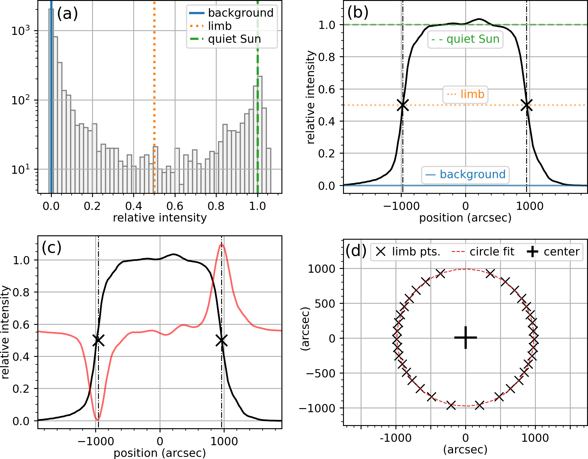
Figure 3: Steps of solar radius measurement. Top panels show the $T\!_{B}$ values distribution of one map (a) and limb points coordinates determination of a single scan by the half-power method(b), where background level corresponds to the solid blue line, limb level corresponds to the dotted orange line, and quiet-Sun level corresponds to the dashed green line; limb points coordinates determination by the inflection-point method(c), where minimum and maximum values of the numerical differentiation of a scan (red curve) correspond to the limb coordinates (black crosses); limb coordinates (black crosses) extracted from a solar map used to fit a circle (red dashed line) and determine the solar radius (d). See also Fig. 2 in Menezes et al. (2021).

In the half-power method, the solar limb is located at the mean $T\!_{B}$ value between the sky background level and the quiet-Sun level, $T\!_{qS}$. The background level is defined as the most common $T\!_{B}$ value, or mode, outside the solar disk (solid blue lines in panels a and b of Fig. 3) and the $T\!_{qS}$value is the $T\!_{B}$ median value in the center of the solar disk (green dashed lines in panels a and b of Fig. 3) constrained within a region of radius of $7.5\mathrm{\prime }$ (blue circle in Fig. 1b). The interpolated points corresponding to the limb level (orange dotted lines in panels a and b of Fig. 3) are the limb coordinates (black $\times$ in panels b and d of Fig. 3).

These extracted limb points are then fit by a circle (red dashed line in panel d of Fig. 3) using a least-squares method to determine the center coordinates. The radius, $R_{\theta}$, of each map is calculated as the average of the center-to-limb distances.

As described by Menezes et al. (2021), some criteria are adopted to avoid extracting limb points associated with active regions and instrumental or random observational errors introduced by high Earth’s atmospheric attenuation. For the limb point extraction, only those with a center-to-limb distance between $815\mathrm{″}$ ($0.85$ $R_{\theta}$) and $1100\mathrm{″}$ ($1.15$ $R_{\theta}$) are considered. During the radius calculation, successive circle fits are made. For each fit, the points with center-to-limb distance, $r$, outside the interval $\bar{R}-$$<r<\bar{R}+$$$ are discarded, and then a new circle fit is performed with the remaining points. This process is repeated until no other point is discarded. If there are less than 10 points (out of the usual 34) remaining, the entire map is discarded; otherwise, the radius is calculated. If the standard deviation is below $20\mathrm{″}$, then the calculated radius is stored and the next map is submitted to this process. The same method was applied to the data from both telescopes.

Over 3000 solar maps observed within the period of 2015-2018 were analyzed and the results of the radius determination for each frequency are listed on Table 1 for both the half-power method and the inflection-point method. Also listed on the last two columns of Table 1 are the predicted values of the solar radius, R_ssc, and the respective convolved values, $R_{\mathrm{ssc}}^{\mathrm{conv}}$, using the SSC atmospheric model (Selhorst et al., 2005), further explained in the next section.

The solar radius results (Table 1) indicated that the half-power method yield larger radius values when compared to the inflection-point method – the values derived from ALMA maps are about $1\mathrm{″}$ larger, while the ones derived from SST maps are about $10\mathrm{″}$ larger. Also, the inflection-point method radii are closer to the radius measurements reported in the literature (Selhorst et al., 2019a; Alissandrakis et al., 2020; Menezes et al., 2021). Moreover, considering the uncertainties, the radii are in agreement with the SSC model radius predictions, R_ssc and $R_{\mathrm{ssc}}^{\mathrm{conv}}$, except R_ssc at 100 GHz and $R_{\mathrm{ssc}}^{\mathrm{conv}}$ at 212 GHz.

Table 1: Average radii at sub-THz frequencies determined using the half-power method and the inflection-point method, and radii derived from SSC model.

Frequency	Half-power	Inflection-point
(GHz)	$\bar{R}$ (′′)	$\bar{R}$ (′′)	Rssc (′′)	$R_{\mathrm{ssc}}^{\mathrm{conv}}$ (′′)
100 (ALMA)	$969\pm 2$	$968\pm 3$	964.2	966.4
212 (SST)	$967\pm 3$	$963\pm 3$	963.6	969.0
230 (ALMA)	$964.1\pm 1.7$	$963\pm 2$	963.5	965.0
405 (SST)	$965\pm 5$	$963\pm 5$	962.9	967.4

4 Limb brightening

4.1 Simulated T_B profiles

Atmospheric solar models, such as the SSC model (Selhorst et al., 2005) – a 2-D solar atmospheric model, which takes into account the curvature of the Sun and may include spicules – predict limb brightening of the solar disk at sub-THz frequencies. High $L\!B$ of the solar disk and the antenna beam shape can affect the determination of the radius that could be overestimated, while $L\!B$ could be underestimated. To investigate this, we simulated single scans over the solar disk, which consist of 1-D convolutions of the beam profiles with the synthetic $T\!_{B}$ profiles. The synthetic profiles are generated by scaling SSC profiles with limb brightening levels above quiet-Sun level, $L\!B$_synth, from 0 to 40% (in 5% steps), and radius, R_synth, from $960\mathrm{″}$ to $976\mathrm{″}$ (varying by $1\mathrm{″}$), resulting in a total of 153 $T\!_{B}$ profiles. Examples of the SSC $T\!_{B}$ profiles (red curves) convolved with SST and ALMA’s beam profiles (gray curves) are shown in Fig. 4 as a black curve.

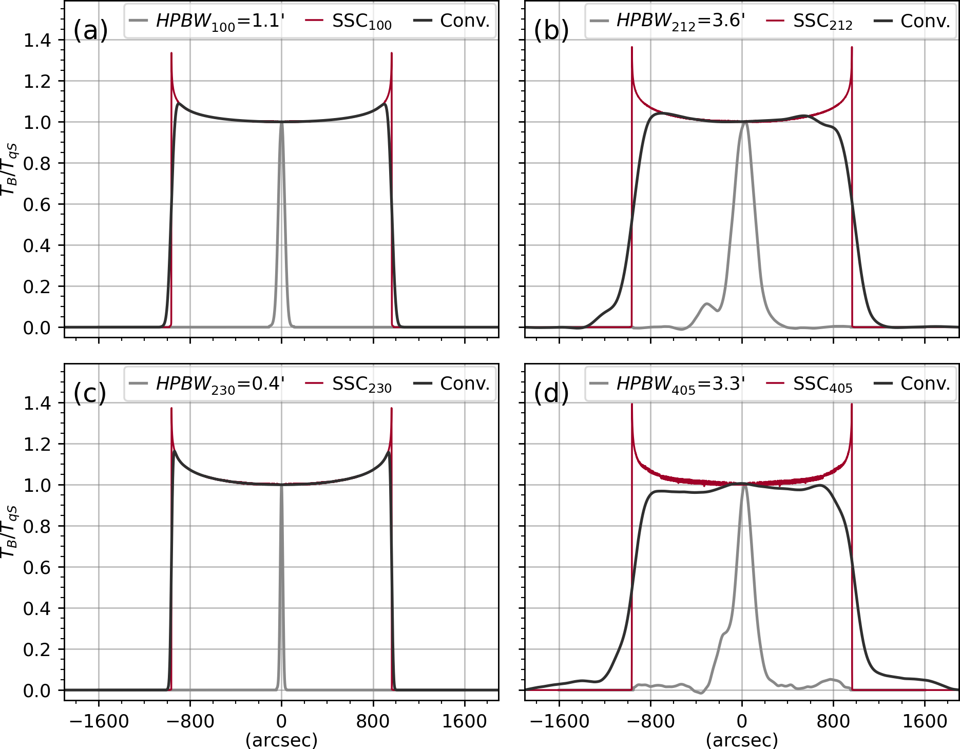
Figure 4: Convolved $T\!_{B}$ profiles (black lines) from the convolution of the telescope beams (gray lines) and the SSC $T\!_{B}$ profiles (red lines) at 100 (a), 212 (b), 230 (c), and 405 GHz (d).

After the convolution, the radius, R_conv, of the convolved $T\!_{B}$ profile is calculated both by the half-power method and by the inflection-point method. Then R_synth is subtracted from R_conv to determine the difference, $\Delta\!R$, the height above the photosphere. By varying R_synth for the same $L\!B$_synth value, $\Delta\!R$ remains with the same value; also, for $L\!B$_synth= 0%, $\Delta\!R$ is negligible. In addition to the radius, the limb brightening level, $L\!B$_conv, of the convolved profiles are also determined in order to assess the $L\!B$ decrease after the beam convolution.

Next we estimate a possible range of $L\!B$ for each average radius, $\bar{R}$. First, for each R_synth, we select the four R_conv closest to $\bar{R}$. From these four values, only those in the range $\bar{R}$$-\sigma\leq\textit{R}\textsubscript{conv}\leq$$\bar{R}$$+\sigma$ are considered, where $\sigma$ is the standard deviation of $\bar{R}$ for each frequency. Then, we select the $L\!B$ of the $T\!_{B}$ profiles that corresponds to these valid R_conv. Moreover, two linear fits are performed: one with the lowest $L\!B$ of each R_synth, and another onefor the highest $L\!B$ of each R_synth, resulting in a $L\!B$ band that ranges from 0% to 40%, as a function of R_synth. Finally, we select the lower and the upper value of $L\!B$ band for the $\bar{R}$ of the solar disk, thus estimating a $L\!B$ range.

4.2 Limb brightening estimate

In addition to the radius, $L\!B$ is also affected by the shape of the antenna beam. In Fig. 4 and Table 2, the $L\!B$ obtained from the SSC $T\!_{B}$ profiles are much higher than $L\!B$_conv of the respectively convolved profiles. In the case of the $T\!_{B}$ profiles at 212 and 405 GHz, $L\!B$_conv is very low and the convolved profiles are asymmetric, which are a result of wider beams with high secondary lobes. The decrease in $L\!B$ can also be seen in Table 2 that lists $L\!B$_conv, and in Fig. 5 that shows the decrease, $\Delta\!L\!B$ ($L\!B$_synth – $L\!B$_conv), for the respective $L\!B$_synth.

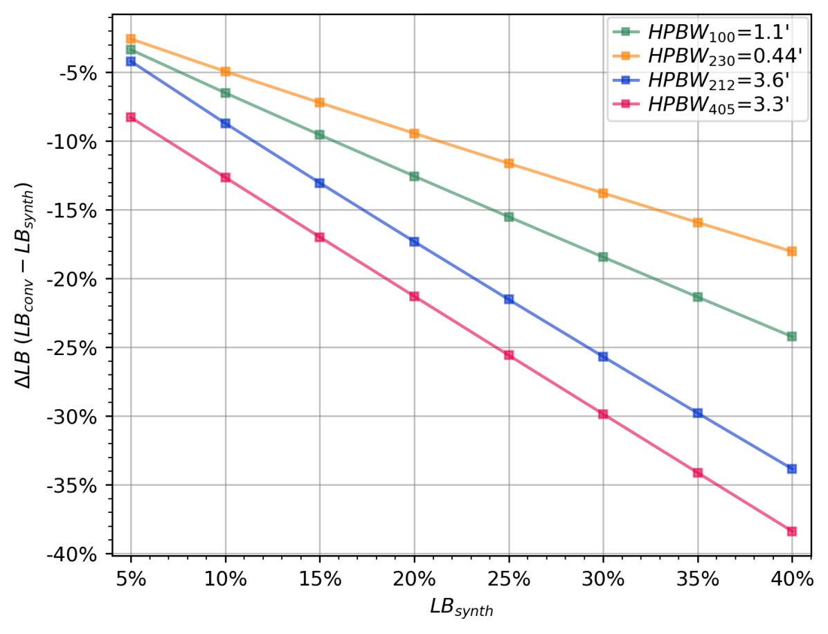
Figure 5: Limb brightening decrease, $\Delta\!L\!B$ ($L\!B$_synth – $L\!B$_conv), for the respective $L\!B$_synth, at 100 GHz (green), 230 GHz (yellow), 212 GHz (blue) and 405 GHz (red).

We use the R_conv calculated by the inflection-point method to estimate a band of possible $L\!B$ for each frequency, by performing several solar scan simulations. The bands of $L\!B$ as a function of the solar radius, R_synth, are shown in Fig. 6. For example, the $L\!B$ at 230 GHz has an upper limit that ranges from 40% to 0% for R_synth in the interval from $\sim$$960.5\mathrm{″}$ to $\sim$$965.5\mathrm{″}$; whereas the lower limit ranges from 25% to 0% for a R_synth range within $960\mathrm{″}$ to $\sim$$964.2\mathrm{″}$. Therefore, based on the lower and upper limits and on $\bar{R}$ (average radii), $L\!B$ estimate at 230 GHz ranges from 6.4% to 17.6%.

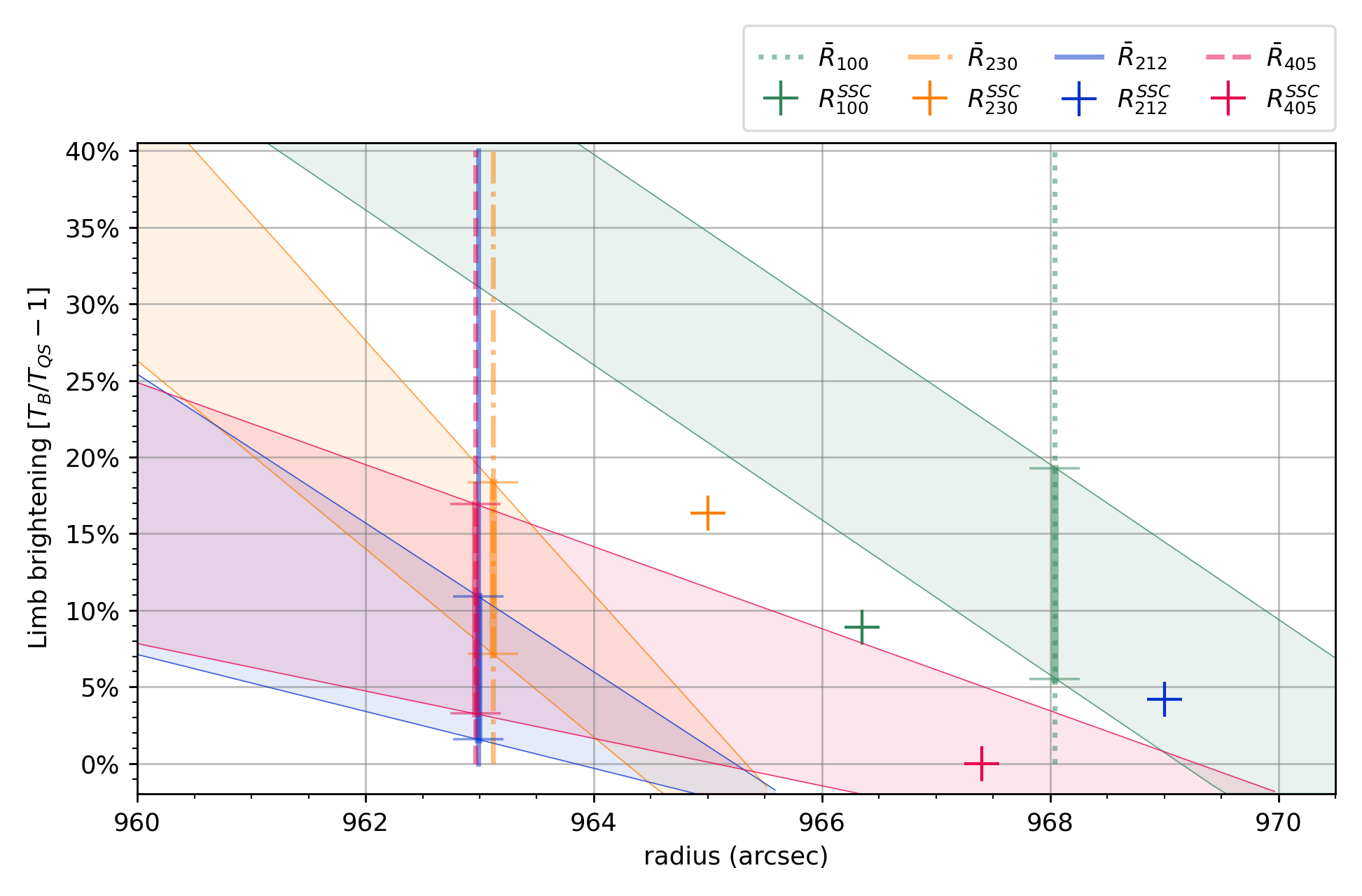
Figure 6: Limb brightening, $L\!B$, estimate bands (semitransparent colors) as a function of solar radius derived from the inflection-point method. The crosses are the model predicted radii, R_ssc, and limb brightening levels, $L\!B$, derived from the SSC $T\!_{B}$ profiles convolved with the beams. The vertical lines are the observed average radii, $\bar{R}$, at 100 (dotted green line), 212 (solid blue line), 230 (dashed-dotted yellow line) and 405 GHz (dashed red line). Each frequency is represented by the colors green (100 GHz), blue (212 GHz), yellow (100 GHz) and red (405 GHz).

Table 2: Limb brightening levels derived from SSC model, and limb brightening estimates based on the average radii.

Frequency		$L\!B$ for $\bar{R}$		SSC model
(GHz)		(%)		$L\!B$ (%)	$L\!B$conv(%)
100 (ALMA)		5.0 - 18.7		33.6	8.9
212 (SST)		1.6 - 12.0		36.5	4.2
230 (ALMA)		6.4 - 17.6		37.4	16.3
405 (SST)		3.3 - 17.0		39.3	3.2

In Table 2, $L\!B$ estimate ranges based on $\bar{R}$ (average radii) are listed. The $L\!B$ ranges at 100 and 230 GHz agree with the values reported by Selhorst et al. (2019b). At 212 and 405 GHz, there are no measured values, because the SST beams are too wide and, hence, no $L\!B$ are seen in the solar maps. However, considering the proximity in frequency to 230 GHz, the $L\!B$ range at 212 GHz contains the $L\!B$ at 230 GHz reported by Selhorst et al. (2019b).

The $L\!B$ ranges estimate do not agree with the $L\!B$ derived from SSC’s $T\!_{B}$ profiles (second last column of Table 2), which predicts a much higher $L\!B$. Nevertheless, $L\!B$_conv (last column of Table 2) derived from the convolved SSC model $T\!_{B}$ profiles are within the estimate ranges, except at 405 GHz, that shows a lower $L\!B$_conv  albeit very close to the lower limit. As stated in Section 2.3, SST beams asymmetyr and large FWHD could explain such low $L\!B$. Also, SSC profiles $L\!B$_conv at 100 and 230 GHz are respectively lower, however close to the 10.5% and 17.8% levels reported by Selhorst et al. (2019b).

4.3 Limb brightening versus radius determination method

The discrepancies between both methods are more evident in Table 3 and in Fig. 7. Values of R_conv and $L\!B$_conv of the convolved profiles are listed in Table 3. Fig. 7 shows the radius increases, $\Delta\!R$, i. e. the difference between the radii of the $T\!_{B}$ profiles, R_synth, and the convolved profiles, R_conv. In the top panel, $\Delta\!R$ is shown as a function of $L\!B$, and in the bottom panel, as a function of HPBW. This confirms that the measured radii are affected by the shape of the beam and $T\!_{B}$ profiles.

Table 3: Values of $L\!B$_conv and R_conv derived from 1-D convolutions of beam profiles and synthetic $T\!_{B}$ profiles.

Beam	$L\!B$synth	$L\!B$conv	Half-power	Inflection-point
	($T\!_{B}$$/$$T\!_{qS}$$-1$)	($T\!_{B}$$/$$T\!_{qS}$$-1$)	Rconv (′′)	Rconv (′′)
100 GHz	5%	1.6%	965.4	964.7
HPBW=$1.1\mathrm{\prime }$	10%	3.5%	966.4	965.0
Rsynth=$964.2\mathrm{″}$	15%	5.5%	967.4	965.4
	20%	7.5%	968.3	965.7
	25%	9.5%	969.2	966.0
	30%	11.6%	970.1	966.3
	35%	13.7%	970.9	966.6
	40%	15.8%	971.7	966.8
212 GHz	5%	0.8%	966.3	964.7
HPBW=$3.6\mathrm{\prime }$	10%	1.3%	968.8	965.7
Rsynth=$963.6\mathrm{″}$	15%	2.0%	971.3	966.6
	20%	2.7%	973.7	967.5
	25%	3.5%	976.0	968.3
	30%	4.3%	978.2	969.1
	35%	5.2%	980.4	969.9
	40%	6.2%	982.5	970.6
230 GHz	5%	2.4%	964.1	963.8
HPBW=$0.44\mathrm{\prime }$	10%	5.1%	964.6	964.1
Rsynth=$963.5\mathrm{″}$	15%	7.8%	965.1	964.3
	20%	10.6%	965.5	964.5
	25%	13.4%	966.0	964.8
	30%	16.2%	966.4	964.9
	35%	19.1%	966.7	965.1
	40%	22.0%	967.1	965.3
405 GHz	5%	-3.3%	965.5	963.7
HPBW=$3.3\mathrm{\prime }$	10%	-2.6%	967.8	964.4
Rsynth=$962.9\mathrm{″}$	15%	-2.0%	970.1	965.0
	20%	-1.3%	972.2	965.7
	25%	-0.6%	974.4	966.3
	30%	0.1%	976.4	966.9
	35%	0.9%	978.4	967.5
	40%	1.6%	980.3	968.0

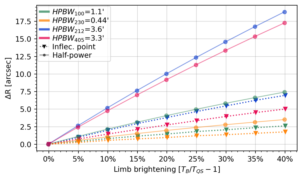
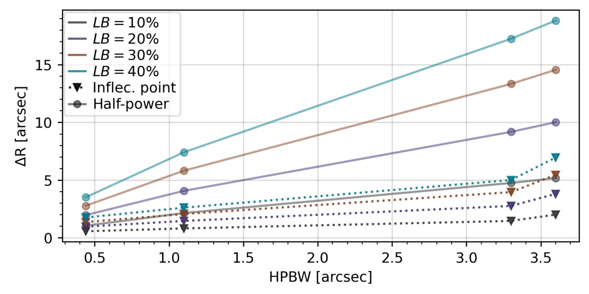
Figure 7: Radius increases, $\Delta\!R$, calculated as the subtraction, $\textit{R}\textsubscript{conv}-\textit{R}\textsubscript{synth}$, of the synthetic profile radius from the convolved profiles. Top panel: $\Delta\!R$ for each beam profile is represented by green (100 GHz), yellow (230 GHz), blue (212 GHz) and red (405 GHz) lines. Bottom panel: $\Delta\!R$ for each limb brightening level, $L\!B$, is represented by black ($L\!B$ = 10%), purple (20%), brown (30%) and turquoise (40%) lines. In both panels, the solid color lines with circles represent $\Delta\!R$ derived from the half-power method, whereas the dotted color lines with inverted triangles represent $\Delta\!R$ derived from the inflection-point method.

In both methods, $\Delta\!R$ increases with both $L\!B$ and HPBW. However, $\Delta\!R$ is larger when the half-power method is used, being less pronounced for narrow HPBW and more pronounced for wider HPBW. This means that the inflection-point method is less susceptible to the shape of the beam and $T\!_{B}$ profiles. Therefore, the inflection-point method carries less bias to the calculation of the solar radius and should thus be preferred for radius determination.

5 Conclusions

In this work we determine the average radius of the full solar disk at 100, 212, 230, and 405 GHz, using data from SST and ALMA’s single-dish observations. We compare the half-power method and the inflection-point method to find which one is more suitable for this kind of measurement. By performing solar scans simulations (1-D convolutions), we identify how the $L\!B$ in $T\!_{B}$ profiles and the HPBW of the antennas inflict larger bias in the measurements. Moreover, we use the simulation output to estimate ranges of probable $L\!B$ for solar $T\!_{B}$ profiles observed at sub-THz frequencies.

The solar scan simulation estimates of $\Delta\!R$ indicated that the combination of solar limb brightening in association with the radio-telescope beam width and shape can affect the radius determination depending on the method used. We found that the inflection-point method is less prone to the irregularities of the telescope beam and to the variations of the $L\!B$ profile of the Sun. In conclusion, the inflection-point method results in a lower bias in solar radius determination and, therefore, is more suitable for such task.

The higher precision solar radii calculation allowed us to investigate the presence of limb brightening and estimate $L\!B$ of the Sun at sub-THz frequencies. This is done by simulating $T\!_{B}$ profiles with varying $L\!B$ and convolving them with the measured beam profiles. The limb brightening determination from solar scan simulations yields ranges of $L\!B$ that agree with previous measurements (100 and 230 GHz, Selhorst et al., 2019b) and is able to estimate $L\!B$ from low spatial resolution solar maps such as those from SST. However, the values are not in agreement with the $T\!_{B}$ profiles generated by the SSC model.

As stated by Selhorst et al. (2019b), some observations reported brightening values much smaller than the expected values predicted by the models, with discrepancies being particularly large at millimeter wavelengths. Those discrepancies could be due to the presence of chromospheric features such as spicules located close to the limb or, in the case of SST maps, probably due to the large beam width and deformations. In fact, the model represents average approximations, which do not always reproduce the observations.

Measurements of the Sun at radio frequencies with high precision can be difficult, since it depends directly on high spatial resolution solar maps. In spite of that, we were able to determine the solar radius and estimate the limb brightening at sub-THz frequencies. Our results are crucial to test and improve solar atmospheric models, and better understand the solar atmosphere, since they probe directly different low lying atmospheric layers. More studies of this kind at other radio frequencies are needed to achieve such objectives.

Data Availability

The data from the Solar Submillimeter-wave Telescope (SST) underlying this article were provided by the Center for Radio Astronomy and Astrophysics Mackenzie (CRAAM) by permission. Data will be shared upon request to the corresponding author with permission of CRAAM.

The data from the Atacama Large Millimeter/submillimeter Array (ALMA) underlying this article are available in ALMA Science Verification Data page at https://almascience.eso.org/alma-data/science-verification (ADS/JAO.ALMA #2011.0.00020.SV), and in ALMA Science Archive page at http://almascience.eso.org/asax/ (the rest of ALMA data).

References

- Alissandrakis et al. (2017) Alissandrakis C. E., Patsourakos S., Nindos A., Bastian T. S., 2017, A&A, 605, A78
- Alissandrakis et al. (2020) Alissandrakis C. E., Nindos A., Bastian T. S., Patsourakos S., 2020, A&A, 640, A57
- Antia (1998) Antia H., 1998, Astronomy & Astrophysics, 330, 336
- Auwers (1891) Auwers A., 1891, Astronomische Nachrichten, 128, 361
- Brown & Christensen-Dalsgaard (1998) Brown T. M., Christensen-Dalsgaard J., 1998, ApJ, 500, L195
- Brown et al. (1982) Brown T. M., Elmore D. F., Lacey L., Hull H., 1982, Appl. Opt., 21, 3588
- Coates (1958) Coates R. J., 1958, ApJ, 128, 83
- Costa et al. (1999) Costa J. E. R., Silva A. V. R., Makhmutov V. S., Rolli E., Kaufmann P., Magun A., 1999, ApJ, 520, L63
- Costa et al. (2002) Costa J., Silva A. R., Lüdi A., Magun A., 2002, Astronomy & Astrophysics, 387, 1153
- Emilio et al. (2000) Emilio M., Kuhn J. R., Bush R. I., Scherrer P., 2000, ApJ, 543, 1007
- Fontenla et al. (1993) Fontenla J. M., Avrett E. H., Loeser R., 1993, ApJ, 406, 319
- Gilliland (1981) Gilliland R. L., 1981, ApJ, 248, 1144
- Giménez de Castro et al. (2020) Giménez de Castro C. G., Pereira A. L. G., Valle Silva J. F., Selhorst C. L., Mand rini C. H., Cristiani G. D., Raulin J.-P., Valio A., 2020, arXiv e-prints, p. arXiv:2009.03445
- Horne et al. (1981) Horne K., Hurford G. J., Zirin H., de Graauw T., 1981, ApJ, 244, 340
- Kaufmann et al. (2008) Kaufmann P., et al., 2008, in Ground-based and Airborne Telescopes II. p. 70120L, doi:10.1117/12.788889
- Kilcik et al. (2009) Kilcik A., Sigismondi C., Rozelot J., Guhl K., 2009, Solar Physics, 257, 237
- Kosovichev & Rozelot (2018) Kosovichev A., Rozelot J.-P., 2018, ApJ, 861, 90
- Kubo (1993) Kubo Y., 1993, Publications of the Astronomical Society of Japan, 45, 819
- Lindsey & Hudson (1976) Lindsey C., Hudson H. S., 1976, ApJ, 203, 753
- Lindsey et al. (1981) Lindsey C., Hildebrand R. H., Keene J., Whitcomb S. E., 1981, ApJ, 248, 830
- Menezes & Valio (2017) Menezes F., Valio A., 2017, Sol. Phys., 292, 195
- Menezes et al. (2021) Menezes F., Selhorst C. L., Giménez de Castro C. G., Valio A., 2021, ApJ, 910, 77
- Nakajima et al. (1994) Nakajima H., et al., 1994, IEEE Proceedings, 82, 705
- Rozelot et al. (2018) Rozelot J. P., Kosovichev A. G., Kilcik A., 2018, Sun and Geosphere, 13, 63
- Selhorst et al. (2003) Selhorst C. L., Silva A. V. R., Costa J. E. R., Shibasaki K., 2003, A&A, 401, 1143
- Selhorst et al. (2005) Selhorst C. L., Silva A. V. R., Costa J. E. R., 2005, A&A, 433, 365
- Selhorst et al. (2011) Selhorst C. L., Giménez de Castro C. G., Válio A., Costa J. E. R., Shibasaki K., 2011, ApJ, 734, 64
- Selhorst et al. (2019a) Selhorst C. L., Kallunki J., Giménez de Castro C. G., Valio A., Costa J. E. R., 2019a, Sol. Phys., 294, 175
- Selhorst et al. (2019b) Selhorst C. L., et al., 2019b, ApJ, 871, 45
- Shibasaki (1998) Shibasaki K., 1998, in Balasubramaniam K. S., Harvey J., Rabin D., eds, Astronomical Society of the Pacific Conference Series Vol. 140, Synoptic Solar Physics. p. 373
- Swanson (1973) Swanson P. N., 1973, Sol. Phys., 32, 77
- Thuillier et al. (2011) Thuillier G., et al., 2011, Sol. Phys., 268, 125
- Valle Silva et al. (2021) Valle Silva J. F., Giménez de Castro C. G., Selhorst C. L., Raulin J. P., Valio A., 2021, MNRAS, 500, 1964
- Vaquero et al. (2016) Vaquero J. M., Gallego M. C., Ruiz-Lorenzo J. J., López-Moratalla T., Carrasco V. M. S., Aparicio A. J. P., González-González F. J., Hernández-García E., 2016, Sol. Phys., 291, 1599
- Vernazza et al. (1981) Vernazza J. E., Avrett E. H., Loeser R., 1981, ApJS, 45, 635
- White et al. (2017) White S. M., et al., 2017, Sol. Phys., 292, 88
- Withbroe (1970) Withbroe G. L., 1970, Solar Physics, 11, 42
- Wootten & Thompson (2009) Wootten A., Thompson A. R., 2009, IEEE Proceedings, 97, 1463