Quark-diquark potential and diquark mass from Lattice QCD

Abstract

We propose a new application of lattice QCD to calculate the quark-diquark potential, diquark mass and quark mass required for the diquark model. As a concrete example, we consider the $\Lambda_{c}$ baryon and treat it as a charm-diquark($c$-[$ud$]) two-body bound state. We extend the HAL QCD method to calculate the charm-diquark potential which reproduces the equal-time Nambu-Bethe-Salpeter wave function of the S-wave state ($\Lambda_{c}(\frac{1}{2}^{+})$). The diquark mass is determined so as to reproduce the difference between the S-wave and the spin-orbit averaged P-wave energies, i.e. the difference between the $\Lambda_{c}(\frac{1}{2}^{+})$ level and the average of the $\Lambda_{c}(\frac{1}{2}^{-})$ and the $\Lambda_{c}(\frac{3}{2}^{-})$ levels. Numerical calculations are performed on a $32^{3}\times 64$ lattice with lattice spacing of $a\simeq 0.0907$ fm and the pion mass of $m_{\pi}\simeq 700$ MeV. Our charm-diquark potential is given by the Coulomb+linear (Cornell) potential where the long range behavior is consistent with the charm-anticharm potential while the Coulomb attraction is considerably smaller. This weakening of the attraction may be attributed to the diquark size effect. The obtained diquark mass is $m_{D}=1.273(44)$ GeV. Our diquark mass lies slightly above the conventional estimates, namely the $\rho$ meson mass and twice the constituent quark mass $2m_{N}/3$.

I Introduction

Understanding hadrons as quark many-body systems is one of the most important themes in hadron physics. However, solving many-body problems confronts us with numerical complexities even for 3-quark systems. One way to reduce the burden is to introduce a composite particle made of two quarks called the diquark  Gell-Mann (1964); WILCZEK (2005); Jaffe (2005). Then, for instance, a baryon can be considered as a bound state of a diquark and a quark.

Diquark models Santopinto (2005); Lichtenberg et al. (1968, 1982) that reduce the degrees of freedom in this way have been successful in accounting for a wide range of problems, e.g. structures and reactions of hadrons  Galatà and Santopinto (2012); Oettel et al. (1998); Segovia et al. (2015); Jido and Sakashita (2016); Kumakawa and Jido (2017); Chen et al. (2018), exotic hadron levels Maiani et al. (2015); Giannuzzi (2019); Giron and Lebed (2020) and the Regge trajectory in the baryon sector Johnson and Thorn (1976). However, the color confinement imposed by QCD forbids us to conduct direct experimental investigations on the diquark mass, quark-diquark interactions and so on. They are merely inferred for practical calculations Anselmino et al. (1993).

Lattice QCD (LQCD) Monte Carlo calculation, i.e. the first-principle calculation of QCD, makes it possible to study various properties of diquarks. For instance, refs.Hess et al. (1998); Bi et al. (2016) calculated the diquark mass. However, it is still unclear whether the mass evaluated in these references for an isolated diquark is valid in a baryon. Refs.Alexandrou et al. (2006); Francis et al. (2021) calculated the spatial size of the diquark. However, the interaction between a quark and a diquark is still unclear.

Recently, the HAL QCD collaboration proposed a method to calculate hadron-hadron potentials from the equal-time Nambu-Bethe-Salpeter (NBS) wave function Aoki and Doi (2020); Ishii et al. (2007); Iritani et al. (2019) calculated by LQCD. In 2011, Ikeda and Iida applied the HAL QCD method to the quark-antiquark ($q\bar{q}$) system Ikeda and Iida (2012). Their $q\bar{q}$ potential was shown to behave as the well-known Cornell (Coulomb+linear) potential Bali et al. (2005, 2005); Bali (2001); Eichten et al. (1975). However, Ikeda and Iida set the quark mass to half of the vector meson mass based on a naive constituent quark picture. Kawanai and Sasaki proposed a method to determine the quark mass in 2011 Kawanai and Sasaki (2011, 2015). They did so by imposing a condition on the quark mass by making use of the spin-spin interaction between the quark and the anti-quark. The quark mass calculated by the Kawanai-Sasaki method reproduced the mesonic excitation spectrum with a satisfactory accuracy Nochi et al. (2016); Kawanai and Sasaki (2015). These works together paved a way to evaluating the quark mass and the $q\bar{q}$ interaction potential which are applicable to mesons in general.

This paper extends the works on $q\bar{q}$ to the quark-diquark system, namely baryons. To be specific, we consider the $\Lambda_{c}$ baryon as a two-body system consisting of a charm quark ($c$) and a [$ud$] scalar diquark ($D$). However, the Kawanai-Sasaki method does not work in its original form for the $\Lambda_{c}$ baryon. This is because spin-less scalar diquark and the charm quark do not have spin-spin interaction. Here, we report a novel method to determine the diquark mass, the quark mass and the quark-diquark interaction potential. The condition we impose is that the so-determined quark-diquark potential and the diquark mass reproduce the energy difference between S-wave state ($\Lambda_{c}(\frac{1}{2}^{+})$) and the spin-orbit averaged P-wave states (average of $\Lambda_{c}(\frac{1}{2}^{-})$ and $\Lambda_{c}(\frac{3}{2}^{-})$).

This paper is organized as follows. In Section II, we consider the $q\bar{q}$ system to describe our formalism taking up the charm-anticharm ($c\bar{c}$) system as a specific example. In Section III, we apply our formalism to the $cD$ system where the diquark mass is determined by demanding it to reproduce the P-wave excitation energy of the $\Lambda_{c}$ baryon. In Section IV, we explain the setup of our lattice QCD calculation, i.e. the quark actions, gauge action and the LQCD parameters. Section V shows the numerical results for the $c\bar{c}$ system, namely the $c\bar{c}$ potential and the charm quark mass. Section VI shows the numerical results for the $cD$ system, namely the $cD$ potential and the diquark mass. Section VII compares the $cD$ potential and the $c\bar{c}$ potential. Finally, we summarize our work and give some future prospects in Section VIII.

II Formalism for $q\bar{q}$ sector

In this section, we shall present our formalism for the $q\bar{q}$ system. We focus on the charmonium which is a two-body system of a heavy charm quark ($c$) and an anti-charm quark ($\bar{c}$). Such a system can be treated in the non-relativistic framework so that the interaction between the charm and anti-charm quarks can be expressed by a potential Eichten et al. (1975); Koma and Koma (2013). Its application to other heavy quark systems, such as the bottomium, is straightforward.

II.1 $c\bar{c}$ Numbu-Bethe-Salpeter wave function

We start with the definition of the $c\bar{c}$ equal-time Numbu-Bethe-Salpeter (NBS) wave function $\phi_{\mathcal{M}}(\bm{r})$ for the meson state $\left|{\mathcal{M}}\right\rangle$ in the rest frame, namely

$$\phi_{\mathcal{M}}(\bm{r})\equiv\sum_{\alpha,\beta=1,2,3,4}\left\langle 0\left|\bar{c}_{c,\alpha}(\bm{x})\Gamma_{\mathcal{M},\alpha\beta}c_{c,\beta}(\bm{y})\right|{\mathcal{M}}\right\rangle,$$ (1)

where $|0\rangle$ is the QCD vacuum and $\bm{r}=\bm{x}-\bm{y}$ is the relative coordinate. Here, the operator $c_{c,\alpha}(\bm{x})$ denotes the charm quark field with color $\bm{3}$ index $c$ and spinor index $\alpha$. The composite operator $\bar{c}_{c,\alpha}(\bm{x})\Gamma_{\mathcal{M},\alpha\beta}c_{c,\beta}(\bm{y})$ annihilates the meson $\mathcal{M}$. Contracting the charm and anti-charm quark operators with the Dirac matrix $\Gamma_{\mathcal{M},\alpha\beta}$ specifies the parity and the spin of the annihilation operator. The NBS wave function given by Eq. (1) is gauge dependent since the quark and the antiquark are located at different positions. We fix the gauge to the Coulomb gauge in order to obtain the signal. Representations of the meson $\mathcal{M}$ and the corresponding Dirac matrix $\Gamma_{\mathcal{M},\alpha\beta}$ are summarized in Table 1. For notational simplicity, we omit the spinor and color indices hereafter unless otherwise noted.

Table 1: List of $J^{PC}$, spectroscopic notation ${}^{2S+1}L_{J}$, and Dirac matrix $\Gamma_{\mathcal{M}}$ for the $c\bar{c}$ meson state $\mathcal{M}$.

${\mathcal{M}}$	PS		V		S		AV		T
$J^{PC}$	$0^{-+}$		$1^{--}$		$0^{++}$		$1^{++}$		$1^{+-}$
${}^{2S+1}L_{J}$	${}^{1}S_{0}$		${}^{3}S_{1}$-${}^{3}D_{1}$		${}^{3}P_{0}$		${}^{3}P_{1}$		${}^{1}P_{1}$
$\Gamma_{\mathcal{M}}$	$\gamma_{5}$		$\gamma_{i}$		$I$		$\gamma_{5}\gamma_{i}$		$\gamma_{i}\gamma_{j}$

We define the $c\bar{c}$ potential $\hat{V}_{\mathcal{M}}$ by demanding the NBS wave function to satisfy the following Schrödinger equation in the region $E_{\mathcal{M}}<2M_{{\rm D_{meson}}}$, i.e. below the pair creation threshold of a $D$ meson and a $\bar{D}$ meson Ikeda and Iida (2012); Kawanai and Sasaki (2011):

$$\left(-\frac{\nabla^{2}}{2\mu}+\hat{V}_{\mathcal{M}}\right)\phi_{\mathcal{M}}(\bm{r})=E_{\mathcal{M}}\phi_{\mathcal{M}}(\bm{r}),$$ (2)

where $\mu=m_{c}/2$ is the reduced mass of the $c\bar{c}$ system and $E_{\mathcal{M}}=M_{\mathcal{M}}-2m_{c}$ is the binding energy where $m_{c}$ is the charm quark mass and $M_{\mathcal{M}}$ is the meson mass. At this point, $m_{c}$ is undetermined. This is because the quark cannot be isolated due to the color confinement prohibiting direct measurements of $m_{c}$. Determination of $m_{c}$ will be discussed in the next subsection. On the other hand, the meson mass $M_{\mathcal{M}}$ is extracted from the temporal meson correlator where details will be addressed in Section V.

It is shown in refs.Ikeda and Iida (2012); Kawanai and Sasaki (2011) that the potential operator $\hat{V}_{\mathcal{M}}$ in Eq. (2) is energy-independent and non-local, and acts on the wave function as an integral operator Ishii et al. (2007); Aoki and Doi (2020)

$$\hat{V}_{\mathcal{M}}\psi_{\mathcal{M}}(\bm{r})=\int d^{3}r^{\prime}V_{\mathcal{M}}(\bm{r},\bm{r}^{\prime})\psi_{\mathcal{M}}(\bm{r}^{\prime}).$$ (3)

The derivative expansion Aoki and Doi (2020); Sugiura et al. (2016) $\hat{V}_{\mathcal{M}}(\bm{r},\bm{r}^{\prime})=V_{\mathcal{M}}(\bm{r},\nabla)\delta^{3}(\bm{r}-\bm{r}^{\prime})$ yields

$$V_{\mathcal{M}}(\bm{r},\nabla)=V_{0}(r)+V_{\sigma}(r)\bm{s}_{1}\cdot\bm{s}_{2}+V_{\rm TN}(r)S_{12}+V_{\rm LS}(r)\bm{L}\cdot\bm{S}+O(\nabla^{2}),$$ (4)

where $V_{0}(r)$, $V_{\sigma}(r)$, $V_{\rm TN}(r)$ and $V_{\rm LS}(r)$ denote the spin-independent, spin-spin, tensor and spin-orbit potentials, respectively. The operators $S_{12}\equiv 4\left\{(\bm{r}\cdot\bm{s}_{1})(\bm{r}\cdot\bm{s}_{2})/r^{2}-\bm{s}_{1}\cdot\bm{s}_{2}/3\right\}$, $\bm{s}_{1}$, $\bm{s}_{2}$, $\bm{L}\equiv-i\bm{r}\times\bm{\nabla}$ and $\bm{S}\equiv\bm{s}_{1}+\bm{s}_{2}$ denote the tensor operator, the spin operators for the charm and the anti-charm quarks, the orbital angular momentum operator and the total spin operator, respectively. The higher order term $\mathcal{O}(\nabla^{2})$ is neglected hereafter. Recalling Eq. (3), the integral operator $\hat{V}_{\mathcal{M}}$ in Eq. (2) is replaced by $V_{\mathcal{M}}(\bm{r},\nabla)$.

II.2 Determination of $m_{c}$

Since the charm quark mass in Eq. (2) is undetermined, the $q\bar{q}$ potential is also undetermined at this point. In place of the potential, we first define the pre-potential $\tilde{V}_{\mathcal{M}}(\bm{r})$ by

$$\tilde{V}_{\mathcal{M}}(\bm{r})=\frac{\nabla^{2}\phi_{\mathcal{M}}(\bm{r})}{\phi_{\mathcal{M}}(\bm{r})}.$$ (5)

Recalling Eq. (2), we see that the pre-potential is related to the potential as

$$\tilde{V}_{\mathcal{M}}(\bm{r})\equiv m_{c}\left\{V_{\mathcal{M}}(\bm{r},\nabla)-E_{\mathcal{M}}\right\}.$$ (6)

Hence, the pre-potential is the potential shifted by the binding energy $E_{\mathcal{M}}$ and factorized by $m_{c}$. Explicit forms of the pre-potential for the PS, V, S, AV and T states (see Table 1 for their representations) are obtained as follows. First, $V_{\mathcal{M}}(\bm{r},\nabla)$ in Eq. (6) is replaced by its form given in Eq. (4). Then, the operators $S_{12}$, $\bm{s}_{i}$, $\bm{L}$ and $\bm{S}$ are replaced by their eigenvalues. The results are,

$$\tilde{V}_{\rm PS}(r) = m_{c}\left(V_{0}(r)-(3/4)V_{\sigma}(r)-E_{\rm PS}\right)$$

$$\tilde{V}_{\rm V}(r) \simeq m_{c}\left(V_{0}(r)+(1/4)V_{\sigma}(r)-E_{\rm V}\right)$$

$$\tilde{V}_{\rm S}(r) = m_{c}\left(V_{0}(r)+(1/4)V_{\sigma}(r)-4V_{\rm TN}(r)-2V_{\rm LS}(r)-E_{\rm S}\right)$$

$$\tilde{V}_{\rm AV}(r) = m_{c}\left(V_{0}(r)+(1/4)V_{\sigma}(r)+2V_{\rm TN}(r)-V_{\rm LS}(r)-E_{\rm AV}\right)$$

$$\tilde{V}_{\rm T}(r) = m_{c}\left(V_{0}(r)-(3/4)V_{\sigma}(r)-E_{\rm T}\right).$$ (7)

Here, we have neglected the tensor potential in the V state originating from the small D-wave mixing Nochi et al. (2016).

II.2.1 The Kawanai-Sasaki method for $m_{c}$

Before moving on, we give a brief review of the Kawanai-Sasaki method which is one way to determine $m_{c}$. In this method, it is demanded that the spin-spin interaction potential vanish at long distances, which leads to

$$0 = \lim_{r\to\infty}m_{c}V_{\sigma}(r)$$

$$= \lim_{r\to\infty}\left(\tilde{V}_{\rm V}(r)-\tilde{V}_{\rm PS}(r)-m_{c}\Delta E_{\rm hyp}\right),$$

where $\Delta E_{\rm hyp}\equiv E_{\rm V}-E_{\rm PS}=M_{\rm V}-M_{\rm PS}$. As a result, $m_{c}$ is uniquely determined as

$$m_{c} \equiv \frac{1}{\Delta E_{\rm hyp}}\lim_{r\to\infty}\left(\tilde{V}_{\rm V}(r)-\tilde{V}_{\rm PS}(r)\right)$$ (9)

$$= \frac{1}{\Delta E_{\rm hyp}}\lim_{r\to\infty}\left(\frac{\nabla^{2}\phi_{\rm V}(r)}{\phi_{\rm V}(r)}-\frac{\nabla^{2}\phi_{\rm PS}(r)}{\phi_{\rm PS}(r)}\right)$$

where we have used Eq. (5) to obtain the last line. Note that the Kawanai-Sasaki method requires the spin-spin interaction potential $V_{\sigma}(r)$ to be finite at moderate distances.

II.2.2 A new method to determine $m_{c}$

We propose an alternative method to determine $m_{c}$ without making use of the spin-spin interaction potential. Our strategy is to determine the value of $m_{c}$ so that the Schrödinger equation Eq. (2) reproduces the P-wave excitation energy evaluated using meson masses.

We focus on the spin-singlet sector, i.e. PS and T states which are S-wave and P-wave of our interest. The absence of the spin-orbit potential and the tensor potential in the T state makes the determination of $m_{c}$ simpler compared with the spin triplet sector (see Appendix A for details). Indeed, it is shown from Eq. (7) that the pre-potentials for the PS state and T state are related by

$$\tilde{V}_{\rm T}=\tilde{V}_{\rm PS}+\tilde{E}_{\rm PS,T}.$$ (10)

Here, we have introduced the pre-energy $\tilde{E}_{\rm PS,T}\equiv m_{c}(E_{\rm T}-E_{\rm PS})$. Note that $\tilde{E}_{\rm PS,T}=m_{c}\left(M_{\rm T}-M_{\rm PS}\right)$ follows from the definition of the binding energies $E_{\rm T}$ and $E_{\rm PS}$. We see from Eq. (10) that the only difference between S-wave and P-wave equations is the centrifugal term in the kinetic energy. Hence, we get the following radial part Schrödinger equations:

$$\left(-\frac{1}{r^{2}}\frac{d}{dr}\left(r^{2}\frac{d}{dr}\right)+\tilde{V}_{\rm PS}(r)\right)\phi_{\rm PS}(r) = 0$$

$$\left(-\frac{1}{r^{2}}\frac{d}{dr}\left(r^{2}\frac{d}{dr}\right)+\frac{2}{r^{2}}+\tilde{V}_{\rm PS}(r)\right)\phi_{\rm T}(r) = \tilde{E}_{\rm PS,T}\phi_{\rm T}(r).$$

Now, we proceed as follows. First, we calculate the NBS wave function for the PS state from LQCD using Eq. (1). Next, we construct the pre-potential $\tilde{V}_{\rm PS}(r)$ from the NBS wave function using Eq. (5). Then, we calculate the excitation pre-energy $\tilde{E}_{\rm PS,T}$ by solving the lower of Eq’s.(LABEL:eq:P-wave-excitation). Finally, $m_{c}$ is given by

$$m_{c}\equiv\frac{\tilde{E}_{\rm PS,T}}{M_{\rm T}-M_{\rm PS}}.$$ (12)

III formalism for quark-diquark sector

Next, we formulate our method for the quark-diquark sector. To be specific, we focus on the $\Lambda_{c}$ baryon considering it as a bound state formed by a charm quark and a scalar $[ud]$ diquark ($D$) whose spin, parity, isospin, and color representation are $J^{P}=0^{+}$, $I=0$ and $\overline{\bm{3}}$, respectively. We focus on the S-wave state ($\Lambda_{c}(\frac{1}{2}^{+})$) and the two P-wave states ($\Lambda_{c}(\frac{1}{2}^{-})$ and $\Lambda_{c}(\frac{3}{2}^{-})$) split by the spin-orbit interaction. The spectroscopic notations for the $\Lambda_{c}$ states are summarized in Table 2.

Table 2: Spectrospcopic notations for $\Lambda_{c}$ states as the quark-diquark two-body bound states.

$\Lambda_{c}(J^{P})$	$\Lambda_{c}(\frac{1}{2}^{+})$	$\Lambda_{c}(\frac{1}{2}^{-})$	$\Lambda_{c}(\frac{3}{2}^{-})$
${}^{2S+1}L_{J}$	${}^{2}S_{1/2}$	${}^{2}P_{1/2}$	${}^{2}P_{3/2}$

The outline of our method is as follows. First, we define the $cD$ potential by demanding the $cD$ NBS wave function for the $\Lambda_{c}(\frac{1}{2}^{+})$ state to satisfy a Schrödinger equation. Next, the equation is solved to obtain the LS averaged P-wave excitation energy. Then, the diquark mass is determined by equating the P-wave excitation energy to the difference between $\Lambda_{c}(\frac{1}{2}^{+})$ energy and the spin-orbit average of $\Lambda_{c}(\frac{1}{2}^{-})$ and $\Lambda_{c}(\frac{3}{2}^{-})$ energies.

III.1 cD NBS wave function

Let us start with the $cD$ NBS wave function $\psi_{\Lambda_{c}(J^{P});\alpha}(\bm{r})$ for the $\Lambda_{c}(J^{P})$ state given by

$$\psi_{\Lambda_{c}(J^{P});\alpha}(\bm{r})\equiv\left\langle 0\left|D_{c}(\bm{x})c_{c,\alpha}(\bm{y})\right|\Lambda_{c}(J^{P})\right\rangle,$$ (13)

where $|\Lambda_{c}(J^{P})\rangle$ denotes the $\Lambda_{c}$ baryon state with its spin-parity denoted by $J^{P}$. The composite [$ud$] scalar-diquark operator $D_{c}(\bm{x})$ is defined by

$$D_{c}(\bm{x})\equiv\epsilon_{abc}u_{a}^{T}(\bm{x})C\gamma_{5}d_{b}(\bm{x}),$$ (14)

where $u_{a}(\bm{x})$ ($d_{b}(\bm{x})$) is the field operator of the $u$ ($d$) quark and $C\equiv i\gamma^{2}\gamma^{0}$ the charge conjugation matrix. The Levi-Civita symbol $\epsilon_{abc}$ is introduced to construct the color $\overline{\bm{3}}$ diquark operator. The $cD$ NBS wave function given by Eq. (13) is gauge-dependent. Thus, we fix the gauge before calculating the NBS wave function as in the case of the $c\bar{c}$ system.

We define the $cD$ potential $U(\bm{r},\nabla)$ by demanding the equal-time NBS wave function to satisfy the following Schrödinger equation:

$$\left(-\frac{\nabla^{2}}{2\mu_{cD}}+U(\bm{r},\nabla)\right)\psi_{\Lambda_{c}(J^{P})}(\bm{r})=E_{\Lambda_{c}(J^{P})}\psi_{\Lambda_{c}(J^{P})}(\bm{r}),$$ (15)

where $\mu_{cD}\equiv m_{c}m_{D}/(m_{c}+m_{D})$ is the reduced mass of the $cD$ system and $E_{\Lambda_{c}(J^{P})}\equiv M_{\Lambda_{c}(J^{P})}-(m_{c}+m_{D})$ is the binding energy. Here, $m_{D}$ is the diquark mass to be determined in the next subsection. The mass $M_{\Lambda_{c}(J^{P})}$ of $\Lambda_{c}(J^{P})$ is usually extracted from the corresponding temporal lattice correlator, and will be discussed in Section VI.

The quark-diquark potential $U(\bm{r},\nabla)$ is expressed in terms of the derivative expansion

$$U(\bm{r},\nabla)=U_{0}(r)+U_{\rm LS}(r)\bm{L}\cdot\bm{s},$$ (16)

where $U_{0}(r)$ and $U_{\rm LS}(r)$ denote the central and the spin-orbit potentials, respectively.

III.2 Determination of $m_{D}$

As in the previous section, let us first define the pre-potential $\tilde{U}_{\Lambda_{c}(J^{P})}$ by

$$\widetilde{U}_{\Lambda_{c}(J^{P})}(r)\equiv\frac{\nabla^{2}\psi_{\Lambda_{c}(J^{P})}(\bm{r})}{\psi_{\Lambda_{c}(J^{P})}(\bm{r})}.$$ (17)

Substituting Eq. (16) into Eq. (15) and rearranging with Eq. (17), we arrive at the following equations for $\Lambda_{c}(\frac{1}{2}^{+})$, $\Lambda_{c}(\frac{1}{2}^{-})$ and $\Lambda_{c}(\frac{3}{2}^{-})$ states:

$$\left(-\nabla^{2}+\widetilde{U}_{0}(r)\right)\psi_{\Lambda_{c}(\frac{1}{2}^{+})}(\bm{r}) = 0$$

$$\left(-\nabla^{2}+\widetilde{U}_{0}(r)-\widetilde{U}_{\rm LS}(r)\right)\psi_{\Lambda_{c}(\frac{1}{2}^{-})}(\bm{r}) = 2\mu_{cD}\left(E_{\Lambda_{c}(\frac{1}{2}^{-})}-E_{\Lambda_{c}(\frac{1}{2}^{+})}\right)\psi_{\Lambda_{c}(\frac{1}{2}^{-})}(\bm{r})$$

$$\left(-\nabla^{2}+\widetilde{U}_{0}(r)+\frac{1}{2}\widetilde{U}_{\rm LS}(r)\right)\psi_{\Lambda_{c}(\frac{3}{2}^{-})}(\bm{r}) = 2\mu_{cD}\left(E_{\Lambda_{c}(\frac{3}{2}^{-})}-E_{\Lambda_{c}(\frac{1}{2}^{+})}\right)\psi_{\Lambda_{c}(\frac{3}{2}^{-})}(\bm{r})$$ (18)

where $\widetilde{U}_{0}(r)\equiv 2\mu_{cD}(U_{0}(r)-E_{\Lambda_{c}(\frac{1}{2}^{+})})$ and $\widetilde{U}_{\rm LS}(r)\equiv 2\mu_{cD}U_{\rm LS}(r)$. Here, the eigenvalues of the $\bm{L}\cdot\bm{s}$ operator are used explicitly, namely $0$, $-1$ and $1/2$ for $\Lambda_{c}(\frac{1}{2}^{+})$, $\Lambda_{c}(\frac{1}{2}^{-})$ and $\Lambda_{c}(\frac{3}{2}^{-})$, respectively.

The P-wave pre-energy splits into the following two due to $\tilde{U}_{\rm LS}(r)$:

$$\widetilde{E}_{\rm PW}-\left\langle\widetilde{U}_{\rm LS}\right\rangle_{\rm PW} \simeq 2\mu_{cD}\left(E_{\Lambda_{c}(\frac{1}{2}^{-})}-E_{\Lambda_{c}(\frac{1}{2}^{+})}\right)=2\mu_{cD}\left(M_{\Lambda_{c}(\frac{1}{2}^{-})}-M_{\Lambda_{c}(\frac{1}{2}^{+})}\right)$$

$$\widetilde{E}_{\rm PW}+\frac{1}{2}\left\langle\widetilde{U}_{\rm LS}\right\rangle_{\rm PW} \simeq 2\mu_{cD}\left(E_{\Lambda_{c}(\frac{3}{2}^{-})}-E_{\Lambda_{c}(\frac{1}{2}^{+})}\right)=2\mu_{cD}\left(M_{\Lambda_{c}(\frac{3}{2}^{-})}-M_{\Lambda_{c}(\frac{1}{2}^{+})}\right),$$ (19)

where $\widetilde{E}_{\rm PW}$ is the difference between the pre-energy of the S-wave and the spin-orbit averaged P-wave, i.e. the P-wave eigenvalue of $-\nabla^{2}+\widetilde{U}_{0}(r)$ in the first equation of Eq’s(18). The symbol $\left\langle\widetilde{U}_{\rm LS}\right\rangle_{\rm PW}$ denotes the expectation value of $\widetilde{U}_{\rm LS}(r)$ with respect to the P-wave. We have used the definition of the binding energy $E_{\Lambda_{c}(J^{P})}$ to get the RHS of each equation in Eq’s(19). Solving Eq’s(19) with respect to $\mu_{cD}$, we arrive at

$$\mu_{cD}=\frac{3}{2}\frac{\widetilde{E}_{\rm PW}}{M_{\Lambda_{c}(\frac{1}{2}^{-})}+2M_{\Lambda_{c}(\frac{3}{2}^{-})}-3M_{\Lambda_{c}(\frac{1}{2}^{+})}}.$$ (20)

Once $\mu_{cD}$ is determined, the diquark mass $M_{D}$ is subsequently determined by

$$M_{D}=\frac{\mu_{cD}m_{c}}{m_{c}-\mu_{cD}}.$$ (21)

IV Lattice QCD setup

We use a set of QCD configurations generated by the PACS-CS collaboration Aoki et al. (2009) using the Iwasaki gauge action Iwasaki (2011) and the $\mathcal{O}(a)$-improved Wilson quark action Aoki et al. (2006). The set has 399 of $2+1$ flavor QCD configurations generated on a $V\times T=32^{3}\times 64$ lattice at $\beta=1.90$ with the clover coefficient $c_{{\rm SW}}=1.715$ and the hopping parameters given by $\kappa_{u,d}=0.13700$ for the $u,d$ quarks and $\kappa_{s}=0.13640$ for the $s$ quark Aoki et al. (2009) . The lattice spacing is $a\simeq 0.0907$ fm. The statistical errors are estimated by the standard Jackknife method throughout this paper.

The Iwasaki action for the gauge field is given by

$$S_{{\rm Iwasaki}}\equiv\frac{1}{{\it g}^{2}}\left\{c_{0}\sum_{{\rm plaquette}}{\rm Tr}[U_{{\rm plaq}}]+c_{1}\sum_{{\rm rectangle}}{\rm Tr}[U_{{\rm rect}}]\right\}.$$ (22)

Here, $U_{{\rm rect}}$ denotes the $1\times 2$ rectangle loop of the link variable. The constants are set to $c_{0}=3.648$ and $c_{1}=-0.331$ Iwasaki (2011). Such choice of the coefficients mitigates the discretization errors to $\sim\mathcal{O}(a^{4})$.

The $\mathcal{O}(a)$-improved Wilson quark action $S_{{\rm quark}}$ for the light dynamical quarks ($u,d,s$) is given by

$$S_{{\rm quark}}\equiv \sum_{q=u,d,s}\sum_{x}\left[\bar{q}(x)q(x)\right.$$ (23)

$$-\kappa_{q}c_{{\rm SW}}\sum_{\mu,\nu}\frac{i}{2}\bar{q}(x)\sigma_{\mu\nu}F_{\mu\nu}(x)q(x)$$

$$- \kappa_{q}\sum_{\mu}\left\{\bar{q}(x)(1-\gamma_{\mu})U_{\mu}(x)q(x+\mu)\right.$$

$$+ \left.\left.\bar{q}(x)(1+\gamma_{\mu})U^{\dagger}_{\mu}(x-\mu)q(x-\mu)\right\}\right].$$

Certain choice of the coefficient $c_{{\rm SW}}$ reduces the discretization errors to $\sim\mathcal{O}(a^{2})$. The action Eq. (23) is used to calculate the $u$ quark and $d$ quark propagators.

If we apply the $\mathcal{O}(a)$-improved Wilson quark action designed for light quarks to the heavy charm quark, it yields systematic errors of order $\sim\mathcal{O}(am_{c})$  Aoki et al. (2003). Therefore, we use the relativistic heavy quark action (RHQ)  Aoki et al. (2003); Namekawa et al. (2013) with systematic errors reduced to the same order as the $\mathcal{O}(a)$-improved Wilson quark action. The RHQ action $S_{{\rm RHQ}}$ is given by

$$S_{{\rm RHQ}}\equiv \sum_{x}\bar{Q}(x)Q(x)$$

$$-\kappa_{Q}\sum_{x,y}\bar{Q}(x)$$

$$\Biggl{[}\left.\sum_{i}\left((r_{s}-\nu\gamma_{i})U_{i}(x)\delta_{x+i,y}+(r_{s}+\nu\gamma_{i})U^{\dagger}_{i}(x)\delta_{x,y+i}\right)\right.$$

$$+(r_{t}-\nu\gamma_{4})U_{\hat{4}}(x)\delta_{x+\hat{4},y}+(r_{t}+\nu\gamma_{4})U^{\dagger}_{\hat{4}}(x)\delta_{x,y+\hat{4}}$$

$$+\left.c_{B}\sum_{i,j}F_{ij}(x)\sigma_{ij}+c_{E}\sum_{i}F_{i4}(x)\sigma_{i4}\right]Q(y),$$

where $\hat{4}$ denotes the unit vector in the temporal direction and $Q(x)=c(x)$ denotes the charm quark field. The parameter $r_{t}$ is set to $1$ while other parameters $r_{s},c_{B},c_{E}$ and $\nu$ are taken from Ref. Namekawa et al. (2013) in Table 3.

Table 3: Summary of the parameters used for the RHQ action for the charm quark. The values are taken from Ref. Namekawa et al. (2013).

$\kappa_{c}$	$\nu$	$r_{s}$	$c_{B}$	$c_{E}$
0.10959947	1.1450511	1.1881607	1.9849139	1.7819512

Since we use gauge invariant source and sink operators, the gauge is fixed to the Coulomb gauge. This is done by minimizing the functional $F[U]\equiv\sum_{x}\sum_{i=1}^{3}\left\{{\rm Tr}\left[{\rm Re}U_{i}(x)\right]\right\}$ Gattringer and Lang (2009). This gauge fixing yields discretization errors $\sim O(a^{2})$.

V Numerical results for $c\bar{c}$ system

V.1 Meson mass

Let us start with the meson two-point correlator defined by

$$C^{\mathcal{M}}(t)\equiv\frac{1}{V}\sum_{\bm{x}}\left\langle 0\left|T\left[O^{\mathcal{M}}(\bm{x},t_{{\rm sink}})O^{\mathcal{M}\ \dagger}(t_{{\rm src}})\right]\right|0\right\rangle,$$ (25)

where $V$ is the lattice volume and $t\equiv t_{{\rm sink}}-t_{{\rm src}}$. Here, $O^{\mathcal{M}}=\bar{c}\Gamma_{\mathcal{M}}c$ such that $O^{\mathcal{M}}(\bm{x},t_{{\rm sink}})$ denotes the meson point sink operator and $O^{\mathcal{M}\ \dagger}(t_{{\rm src}})$ denotes the wall source. The Dirac matrix $\Gamma_{\mathcal{M}}$ is chosen accordingly from Table 1.

The time-reversal symmetry $C^{\mathcal{M}}(t)=C^{\mathcal{M}}(T-t)$ is used to reduce the statistical noise for the meson correlator. Also, the statistics improves as the data calculated for 16 different source points $t_{{\rm src}}=0,4,8,\cdots,60$ are averaged. Moreover, the signals of the vector and the axial-vector meson correlators are improved by averaging with respect to the 3-dimensional lattice rotation.

In this work, we employ the periodic boundary condition with respect to $t$. Thus the correlator Eq. (25) acquires the cosh form. Thus, the effective mass $M_{\rm eff}(t)$ is the solution of the following equation

$$\frac{C_{\mathcal{M}}(t+1)}{C_{\mathcal{M}}(t)}=\frac{\cosh\left(M_{\rm eff}(t)\cdot(t+1-T/2)\right)}{\cosh\left(M_{\rm eff}(t)\cdot(t-T/2)\right)},$$ (26)

where $T$ denotes the temporal extension of the lattice.

Fig.1 plots the meson effective mass $M_{\rm eff}(t)$ for PS, V , S, AV, and T states. Then, the meson mass is extracted by fitting the correlator to $f_{\rm fit}(t)\equiv A\cosh(M(t-T/2))$ in each plateau region. The fit is adequately carried out for each channel as shown in the figure with chi-square $\chi^{2}/N_{{\rm d.o.f}}<1.0$, where $N_{{\rm d.o.f}}$ is the number of degrees of freedom in the fit. The meson masses are summarized in Table 4. From the obtained meson masses, we get the hyperfine splitting $\varDelta E_{{\rm hyp}}=M_{\rm{V}}-M_{{\rm PS}}=0.118(1)$ GeV and the P-wave excitation energy for the spin singlet sector $E_{{\rm PS,T}}=M_{{\rm T}}-M_{{\rm PS}}=0.628(16)$ GeV.

For Eq. (2) to be valid, the energy of the $c\bar{c}$ state must be below $2M_{{\rm D-meson}}$. To check this condition, we apply the same procedure to the $D$ meson. The result is $M_{{\rm D-meson}}=1.998(1)$ GeV, thus each $c\bar{c}$ states in Table 4 are bound. For use in Section VI, we also calculate the $\rho$ meson and the pion mass. The results are $M_{\rho}=1.098(5)$ GeV and $M_{\pi}=0.700(1)$ GeV.

Table 4: $c\bar{c}$ meson masses. The fit ranges are shown in the last column.

states	Mass [GeV]	fit range
PS	3.023 (1)	$16\leq t/a\leq 23$
V	3.141 (1)	$16\leq t/a\leq 23$
S	3.546 (11)	$16\leq t/a\leq 23$
AV	3.611 (14)	$16\leq t/a\leq 22$
T	3.651 (16)	$16\leq t/a\leq 23$

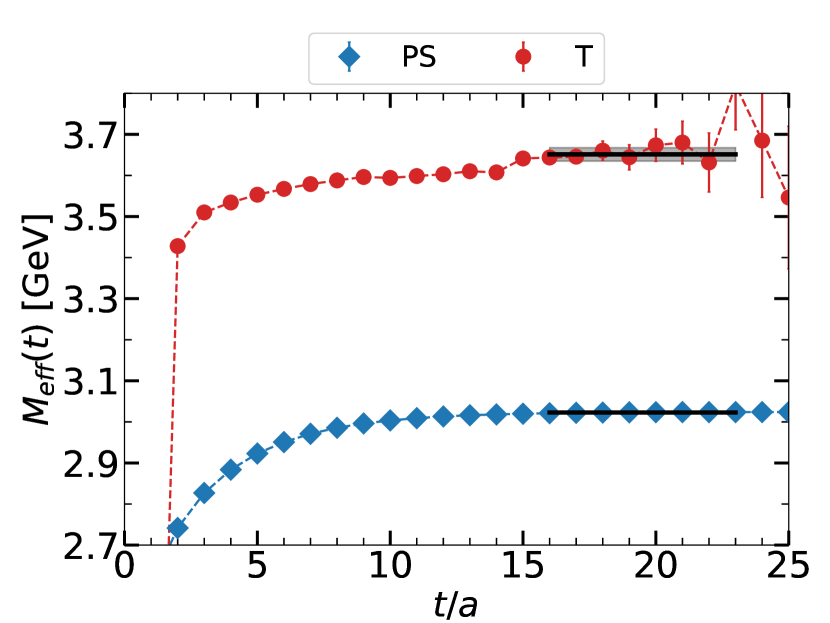
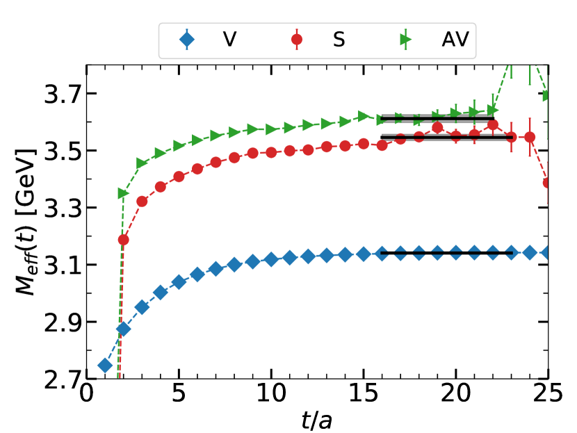
Figure 1: Effective mass plots for the spin singlet (top) and triplet (bottom) sectors. The solid lines denote the average of the meson mass $M_{\mathcal{M}}$ over the fit range. The shaded areas denote the statistical errors estimated by the Jackknife method.

V.2 $c\bar{c}$ NBS wave function

Next, we consider the $c\bar{c}$ four-point correlator  Ikeda and Iida (2012); Kawanai and Sasaki (2011, 2015); Nochi et al. (2016) in the rest frame

$$C_{\mathcal{M}}(\bm{r},t)\equiv\frac{1}{V}\sum_{\bm{\Delta}}$$ (27)

$$\left\langle 0\left|T\left[\bar{c}_{c}(\bm{r}+\bm{\Delta},t_{{\rm sink}})\Gamma_{\mathcal{M}}c_{c}(\bm{\Delta},t_{{\rm sink}})\right.\right.\right.$$

$$\left.\left.\left.\times\mathcal{O}^{\mathcal{M}\ \dagger}(t_{{\rm src}})\right]\right|0\right\rangle.$$

Specifically, we calculate the correlator for the PS and V states, i.e. for $\Gamma_{\mathcal{M}}=\gamma_{5}$ and $\Gamma_{\mathcal{M}}=\gamma_{i}$. Here, the signal of the V state NBS wave function is improved by averaging the vector components symmetric with respect to the 3-dimensional lattice rotation.

Without loss of generality, we restrict ourselves to the $t>0$ region. The four-point function $C_{\mathcal{M}}(\bm{r},t)$ is spectrally decomposed as

$$C_{\mathcal{M}}(\bm{r},t)=\sum_{n}a_{n}\phi_{\mathcal{M}}^{(n)}(\bm{r})e^{-M_{n}t}$$ (28)

where $\phi_{\mathcal{M}}^{(n)}(\bm{r})$, $E_{n}$ and $a_{n}\equiv\langle n|\mathcal{O}^{\mathcal{M}\ \dagger}(0)|0\rangle$ denote the equal-time NBS wave function, the energy and the overlap for the $n$-th excited state $\left|n\right\rangle$, respectively. The energy and the NBS wave function for $n=0$ correspond to the mass and the wave function of the meson state ($\eta_{c}$ for PS and $J/\psi$ for V), respectively. In the large $t$ region, the ground state $\left|0\right\rangle$ becomes dominant as $C_{\mathcal{M}}(\bm{r},t)\sim a_{0}e^{-M_{0}t}\phi_{\mathcal{M}}^{(0)}(\bm{r})$. From now on, we focus on such a region. Next, we project the NBS wave function to the $A_{1}$ representation Lüscher (1991) as

$$\phi_{\mathcal{M}}(\bm{r})=\frac{1}{48}\sum_{g\in O_{h}}\phi_{\mathcal{M}}(g^{-1}\bm{r}),$$ (29)

where $O_{h}$ denotes the cubic group which has 48 elements (see Appendix B). This $\phi_{\mathcal{M}}(\bm{r})$ approximately represents the S-wave. However, there are small contributions from the states with angular momentum $L\geq 4$ that are not removed by the $A_{1}$ projection Ikeda and Iida (2012); Aoki et al. (2005); Sasaki and Ishizuka (2008).

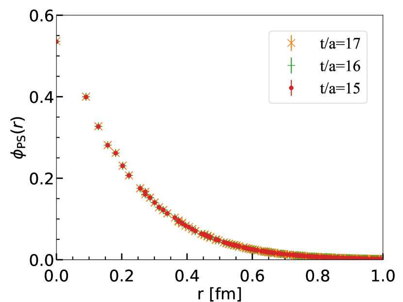
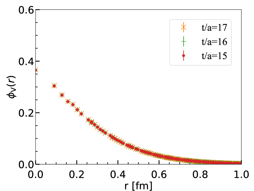
Figure 2: NBS function for the PS (top) and V (bottom) states in $15\geq t/a\geq 17$. The NBS wave function is normalized as $\sum_{r\in V}r^{2}\phi_{\mathcal{M}}^{2}(\bm{r})=1$.

Fig.2 shows the NBS wave function for the PS state and that for the V state in several representative time slices. We see that the NBS wave functions for $t/a=15,16,17$ fall on top of each other. This indicates that the wave function in each time slice has attained its limit $\phi_{\mathcal{M}}(\bm{r})$. We focus on the wave function at $t/a=16$ since the wave functions all coincide in the time region $t/a\geq 15$. Moreover, we focus on the region $0\leq r\leq 1.0$ fm since the NBS wave function is essentially zero beyond 1.0 fm. Note that the NBS wave function has slight rotational symmetry breaking in the short range region. Indeed, the wave function is slightly “jagged” near origin, as shown in Fig.2, which is an indication of the breaking.

This symmetry breaking is due to the discretization errors. Possible sources of errors are the quark actions, the gauge action and the gauge fixing. Since the discretization errors of the gauge action are reduced by an optimal choice of the coefficients, the quark action and the Coulomb gauge fixing will remain to be the main sources of the rotational symmetry breaking.

V.3 Pre-potential for $c\bar{c}$

Next, the pre-potential is evaluated from the NBS wave function according to Eq. (5). Here, the Laplacian is numerically evaluated by the standard nearest-neighbor differentiation

$$\nabla^{2}\phi_{\mathcal{M}}(\bm{r})=\sum_{\hat{\mu}=\hat{i}_{x},\hat{i}_{y},\hat{i}_{z}}\left\{\phi_{\mathcal{M}}(\bm{r}+\hat{\mu})+\phi_{\mathcal{M}}(\bm{r}-\hat{\mu})\right\}-6\phi_{\mathcal{M}}(\bm{r}),$$ (30)

where $\hat{\mu}$ denotes the unit vector in the positive $\mu$-direction and $\hat{i}_{x}$, $\hat{i}_{y}$ and $\hat{i}_{z}$ denote the unit vectors in $x$, $y$ and $z$ directions, respectively.

Fig.3 shows the PS pre-potential and the V pre-potential. These pre-potentials behave roughly as the well-known Coulomb+linear (Cornell) potential as expected. However, we see in Fig.3 that the pre-potential is jagged in the short range region due to the broken rotational symmetry passed on from the NBS wave function.

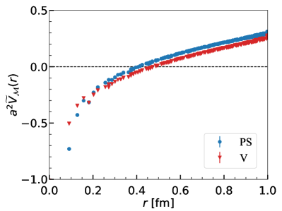
Figure 3: The pre-potentials for the PS (blue dots) and V (red triangles) states.

Next, we fit the pre-potential. Using Eq. (7), the pre-potential is separated into the spin-independent part $\tilde{V}_{0}(r)$ and the spin-spin part $\tilde{V}_{\sigma}(r)$ as

$$\tilde{V}_{0}(r) = m_{q}\left\{V_{0}(r)-\bar{E}_{1S}\right\}=\frac{3}{4}\tilde{V}_{\rm V}(r)+\frac{1}{4}\tilde{V}_{\rm PS}(r)$$

$$\tilde{V}_{\sigma}(r) = m_{q}\left\{V_{\sigma}(r)-\varDelta E_{hyp}\right\}=\tilde{V}_{\rm V}(r)-\tilde{V}_{\rm PS}(r),$$

where $\bar{E}_{1S}=\frac{3}{4}E_{\rm V}+\frac{1}{4}E_{\rm PS}$. We fit the spin-independent part to the Cornell+log function $V^{{\rm fit}}_{0}(r)$ given by

$$V^{{\rm fit}}_{0}(r)=-A/r+Br+C\log(r/a)+v_{0}.$$ (32)

Here, the Cornell term is expected both phenomenologically Eichten et al. (1975) and theoretically Bali et al. (2005) for heavy quark systems. The logarithmic term $C\log(r/a)$ is a correction from the finite quark mass Koma and Koma (2013); Koma et al. (2006); Pérez-Nadal and Soto (2009) where the lattice spacing $a$ is introduced to set the argument dimensionless. The spin-spin part is fit to the 2-Gaussian function $V^{\rm fit}_{\sigma}(r)$ given by

$$V^{\rm fit}_{\sigma}(r)=A_{1}\exp(-B_{1}r^{2})+A_{2}\exp(-B_{2}r^{2})+{v_{\sigma}}.$$ (33)

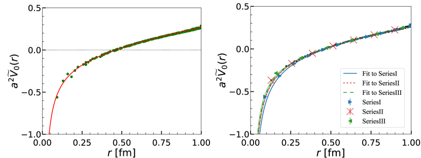
Figure 4: Spin-independent part of the pre-potential (dots) fit to the Cornell+log function (solid line). (left) Fit to ALL and (right) fit to Series I, II and III . The shaded area around each line denotes statistical errors.

First, we fit the spin-independent part of the pre-potential to the Cornell+log function. We fit in the range $1\leq r/a\leq 11$ ($0.09\lessapprox r\lessapprox 1.0$ fm) since the curve is singular at the origin $r=0$. The upper limit is set to $r_{{\rm max}}/a=11$ beyond which the amplitude of the NBS wave function is essentially zero. Hence, the data for the pre-potential becomes meaningless beyond it. Moreover, taking into account the cubic symmetry, we restrict our selves to $x,y,z\geq 0$. The left panel of Fig.4 shows the fit result where we see that most of the points lie close to the curve. However, $\chi^{2}/N_{\rm d.o.f}$ is considerably large, being of the order of $\simeq 1690$. Let us refer to this fit result as “ALL”, and label $\chi^{2}/N_{\rm d.o.f}$ for this as $\left[\chi^{2}/N_{\rm d.o.f}\right]_{\rm ALL}$ in order to distinguish it from other fits which will be presented in the following paragraphs.

One reason for the large $\chi^{2}/N_{\rm d.o.f}$ is the large deviation of the points near origin, namely those at $r/a=1,\sqrt{2},\sqrt{3}$. This is because they are computed by the discretized Laplacian containing the data at the origin which should make sense only in the continuum field theory. Therefore, the data points at and near the origin deviate from the theoretical curve. These points contribute significantly to the large value of $\chi^{2}/N_{\rm d.o.f}$, the sum being estimated to be $\simeq 1460$.

The remaining $\chi^{2}/N_{\rm d.o.f}\simeq 230$ may be attributed to the direction dependence due to RSB. In order to see this point, we fit the spin-independent part for the following three representative directions: Series I ($\bm{r}=(n,0,0)$ ), Series II ($\bm{r}=(n,n,0)$ ) and Series III ($\bm{r}=(n,n,n)$ ) with $n=0,1,2,3\cdots$. There are residual directions with longer periods such as $(n,2n,0)$, but these contributions are less important. In this case, the minimum of the fit range $r_{{\rm min}}$ needs to be determined carefully in order to fit the data adequately. Otherwise, the fit yields unphysical results, e.g. negative Coulomb coefficients. We set $r_{{\rm min}}$ such that $\chi^{2}/N_{{\rm d.o.f}}$ is reasonably small and the fit parameters become stationary. These considerations lead us to the fit range $r_{{\rm min}}/a=4$ ($r_{{\rm min}}\simeq 0.36$ fm). The right panel of Fig.4 shows the spin-independent part of the pre-potential for the three series using the Cornell+log function in this way. Indeed, the fit yields reasonable chi-squares $\chi^{2}/N_{{\rm d.o.f}}\simeq 1.5$, $1.5$ and $0.7$ for Series I, Series II and Series III , respectively. We observe that Series I overestimates the Coulomb attraction near origin, thus separating out clearly from the other two towards the origin.

Now we evaluate the contribution of each series to $\left[\chi^{2}/N_{\rm d.o.f}\right]_{\rm ALL}$. Let us define the chi-square for the three series by

$$\left[\chi^{2}/N_{\rm d.o.f}\right]_{\alpha}\equiv N_{\rm d.o.f}^{-1}\sum_{i}\left[\frac{(y^{\alpha}_{i}-f_{\rm ALL}(r))^{2}}{(\delta y^{\alpha}_{i})^{2}}\right].$$ (34)

Here, $y^{\alpha}_{i}$ denote the $i$-th data point in $\alpha$(= Series I, Series II and Series III ) direction and $\delta y^{\alpha}_{i}$ denotes the statistical error of the data. $\left[\chi^{2}/N_{\rm d.o.f}\right]_{\alpha}$ is approximated by

$$\left[\chi^{2}/N_{\rm d.o.f}\right]_{\rm\alpha}\simeq c_{\alpha}\int_{r_{0}}^{11a}dr\frac{(f_{\alpha}(r)-f_{\rm ALL}(r))^{2}}{(\delta f_{\alpha}(r))^{2}}$$ (35)

where $f_{\alpha}(r)$ is given by $V_{0}^{\rm fit}(r)$ fit to Series $\alpha$. The weight $c_{\alpha}$ is given by $c_{\alpha}=\frac{3}{a},\frac{3}{\sqrt{2}a}$ and $\frac{1}{\sqrt{3}a}$ for Series I, II and III , respectively, considering the density of the data points along each direction. We set the minimum of the integral $r_{0}=(1.5)a,(1.5)\sqrt{2}a,(1.5)\sqrt{3}a$ such that the data points at the tips of the first cubes ($r=a,\sqrt{2}a,\sqrt{3}a$) are excluded from the integral. Note that this approximation assumes each data point is rigorously on the fit curve. On the other hand, the denominator $\delta f_{\alpha}(r)$ is the statistical error for each curve. The error is expressed in terms of the errors of the parameters as

$$\delta f_{\alpha}(r)\simeq\left[(\frac{\delta A}{r})^{2}+(\delta Br)^{2}+(\delta C\log(r))^{2}+\delta v_{0}^{2}\right]^{\frac{1}{2}}.$$ (36)

The results are $\left[\chi^{2}/N_{\rm d.o.f}\right]_{\rm\alpha}\simeq 278$, $\simeq 1.2$ and $\simeq 0.17$, for Series I, Series II and Series III , respectively. The sum $\simeq 279$ is not far from the expected value 230.

Thus, we see that the large value of $\left[\chi^{2}/N_{{\rm d.o.f}}\right]_{\rm ALL}$ for ALL stems from two factors. One is due to the singularity near the origin. The other is due to the direction dependence caused by the RSB. The approach to the continuum limit as $a\to 0$ may then be surmised as follows. The data at the origin approaches negative infinity as $a$ becomes smaller. Since the major error due to the discretized Laplacian is limited to the points ($r=a,\sqrt{2}a,\sqrt{3}a$), it tends to diminish in this limit. Also, importantly, the direction dependence is expected to become smaller by the power $\sim\mathcal{O}(a^{2})$ as $a$ goes to 0. Thus, the fit curve for ALL and those for the three directions approach each other. Overall, the data points will fit to one well-defined curve in the continuum limit.

Next, we fit the spin-spin part of the pre-potential to the 2-Gaussian function in the range $1\leq r/a\leq 10$. Fig.5 shows the fit result. We see that most of the points lye on the curve, and $\chi^{2}/N_{{\rm d.o.f}}\simeq 50.0$. The fit result reproduces the NBS wave function reasonably well, as will be shown in the following subsection.

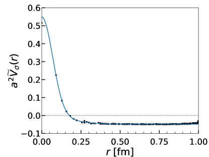
Figure 5: Spin-spin part of the pre-potential fit to 2-Gaussian function (solid line). The black circles denote the pre-potential LQCD data. The flat part of the pre-potential lies below 0 by the amount equal to $m_{c}\varDelta E_{hyp}$.

We refrain from separating the spin-spin part into the three directions because, otherwise, there are too few points that can be used for the fit analysis. Fortunately, the symmetry breaking in the spin-pin part seems to be marginal. This may be because the symmetry breaking in the PS state NBS wave function offsets that in the V state NBS wave function.

V.4 Eigen value problem and the charm quark mass

We put the fit result of the pre-potential $\widetilde{V}^{\rm fit}_{{\rm PS}}(r)=\widetilde{V}^{\rm fit}_{0}(r)-\frac{3}{4}\widetilde{V}^{{\rm fit}}_{\sigma}(r)$ so-obtained into the radial part Schödinger equation Eq. (LABEL:eq:P-wave-excitation):

$$\left[-\frac{1}{r^{2}}\frac{d}{dr}\left(r^{2}\frac{d}{dr}\right)+\left\{\widetilde{V}^{\rm fit}_{{\rm PS}}(r)-\widetilde{E}_{l}\right\}+\frac{l(l+1)}{r^{2}}\right]\phi_{l}(r)=0.$$ (37)

Note that $\phi_{0}(r)=\phi_{{\rm PS}}(r)$, $\widetilde{E}_{0}=0$, $\phi_{1}(r)=\phi_{{\rm T}}(r)$ and $\widetilde{E}_{1}(r)=\widetilde{E}_{{\rm T}}$ follow from Eq. (7). The Discretized Variable Representation (DVR) method Colbert and Miller (1992); Light and Walker (1976) is employed to numerically solve Eq. (37).

We solve the eigenvalue problem using the fit result from ALL. The left panel of Fig.6 compares the numerical result for ALL and the NBS wave function LQCD data. We see that the LQCD data lie close to the numerical solution except at the first two points near origin as expected from the discussions in the previous subsection.

We next use the fit from Series I, Series II and Series III to estimate the direction dependence. The right panel of Fig.6 compares the numerical solution for each series to the LQCD data. The figure shows that the solutions differ in the short range region. According to ref.Aoki et al. (2005), it is not surprising that Series I differs the most from the S-wave . On the other hand, we cannot determine definitively or convincingly which is the better, Series II or Series III within the bounds of numerical precision. For instance, consider the residual sum of squares (RSS) $\delta_{\rm RSS}\equiv\sum_{r}\left\{\phi_{\rm num}(r)-\phi_{\rm NBS}(r)\right\}^{2}$ between the S-wave numerical solution and the NBS wave function. Then, $\sqrt{\delta_{\rm RSS}}\simeq 8\cdot 10^{-2}$, $2\cdot 10^{-2}$, $3\cdot 10^{-2}$ and $5\cdot 10^{-2}$ for Series I, Series II , Series III and ALL, respectively. The last three are of the same order of the numerical precision of the normalization $\simeq 10^{-2}$. See footnote.1 for the marked difference of Series I. The P-wave, on the other hand, is weakly affected by the direction dependence near origin, and thus the solutions for the series coincide.

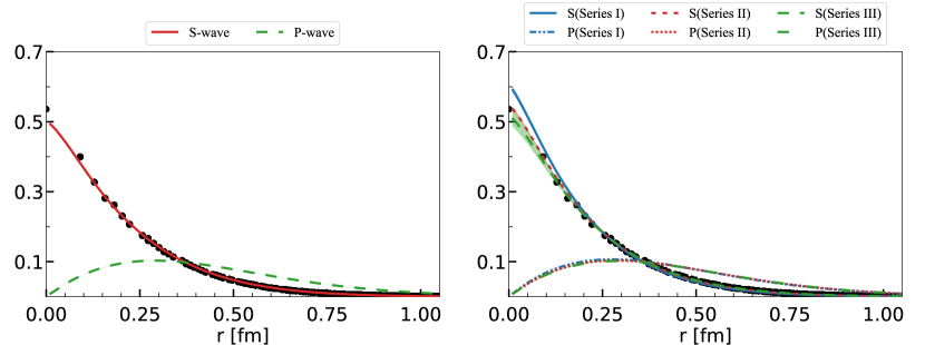
Figure 6: Numerical solutions for S-wave (S) and P-wave (P) compared with the LQCD data (black dots). (left) from ALL and (right) from Series I, II and III . Each shaded area denotes the statistical error.

Using the excitation pre-energy $\tilde{E}_{{\rm PS,T}}$, the charm quark mass is given by $m_{c}=\frac{\tilde{E}_{{\rm PS,T}}}{M_{{\rm T}}-M_{{\rm PS}}}$. Table 5 summarizes $m_{c}$ where we see that each mass lies between $1.9$ GeV and $1.7$ GeV. The difference of $\sim 200$ MeV is the systematic error due to the RSB. Fig.7 compares the charm quark mass for ALL, Series I, Series II and Series III with that obtained from the Kawanai-Sasaki method $m_{c}=1.933(17)$ GeV. In the figure, we see that our result and the value from the Kawanai-Sasaki method roughly agree. The slight difference comes from the fact that our method uses the P-wave excitation energy while the Kawanai-Sasaki method uses the hyperfine splitting. Following the convention, we use the charm quark mass obtained from ALL hereafter for necessary conversions since there is no definitive choice among the three directions within the bounds of numerical precision.

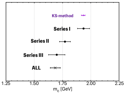
Figure 7: Charm quark mass from ALL and SeriesI, II , III compared to that of the Kawanai-Sasaki method.

Table 5: Summary of the charm quark mass.

directions	ALL	Series I	Series II	Series III
$m_{c}$ [GeV]	1.686 (44)	1.936 (53)	1.771 (48)	1.699 (73)

Using the charm quark mass $m_{c}=1.686(44)$ GeV and the pre-potential, the potential is given by $V_{0}(r)=\frac{1}{m_{c}}\tilde{V}_{0}(r)+\overline{E}_{1S}$. Table 6 summarizes the result of the coefficients of the Cornell+log function $F(r)=-\frac{A}{r}+Br+C\log(r/a)+v_{0}$ fit to ALL and Series I, II and III . The Coulomb coefficient $A$ depends strongly on the direction because it is determined in the short range region as noted before. On the other hand, the coefficients $B$, $C$ and $v_{0}$ have smaller direction dependence since they are determined from the long range region.

The spin-spin potential is given by $V_{\sigma}(r)=\frac{1}{m_{c}}\tilde{V}_{\sigma}(r)+\varDelta E_{\rm hyp}$. The parameters of the 2-Gauss function Eq. (33) fit to the spin-spin potential are $A_{1}=0.135(4)$ GeV, $B_{1}=19.34(38)$ fm^-2, $A_{2}=1.540(41)$ GeV, $B_{2}=104.7(4)$ fm^-2 and $v_{\sigma}=-0.0170(38)$ GeV.

Table 6: Summary of the parameters for the Cornell+log function fit to the spin-independent part of the $c\bar{c}$ potential.

direction	$A$ [GeV$\cdot$fm]	$B$ [GeV/fm]	$C$ [GeV]	$v_{0}$ [GeV]
ALL	0.080(2)	0.748(26)	0.328(14)	-0.964(70)
Series I	0.118(4)	0.647(28)	0.331(11)	-0.856(74)
Series II	0.098(4)	0.695(37)	0.312(11)	-0.867(74)
Series III	0.089(9)	0.737(60)	0.300(16)	-0.880(75)

VI Numerical results for $cD$ system

VI.1 $\Lambda_{c}$ mass

Let us start with the $\Lambda_{c}(\frac{1}{2})$ baryon correlator $C^{\frac{1}{2}}_{\alpha\beta}(t)$ given by

$$C^{\frac{1}{2}}_{\alpha\beta}(t)\equiv\frac{1}{V}\sum_{\bm{x}}\left\langle 0\left|T\left[\mathcal{B}_{\alpha}(\bm{x},t_{{\rm sink}})\overline{\mathcal{B}}_{\beta}(t_{{\rm src}})\right]\right|0\right\rangle,$$ (38)

where $\mathcal{B}_{\alpha}=\left[u^{T}C\gamma_{5}d\right]c_{\alpha}$ such that $\mathcal{B}_{\alpha}(\bm{x},t_{{\rm sink}})$ denotes the $\Lambda_{c}(\frac{1}{2})$ point sink operator and $\overline{\mathcal{B}}_{\alpha}(t_{{\rm src}})$ denotes the wall source operator. The operator $\mathcal{B}_{\alpha}(\bm{x},t)$ couples to both positive parity and negative parity states. Therefore, the correlator has components corresponding to the propagation between the opposite parity states as well as between the same parity states. To eliminate the propagation between the opposite parity states, we act the projection operator $P^{\pm}_{\alpha\beta}=\left[\frac{\bm{1}\pm\gamma_{0}}{2}\right]_{\alpha\beta}$ to $C^{\frac{1}{2}}_{\alpha\beta}(t)$ as

$$C^{\frac{1}{2}^{\pm}}(t)=\sum_{\alpha,\beta}P^{\pm}_{\alpha\beta}C^{\frac{1}{2}}_{\alpha\beta}(t),$$ (39)

where $C^{\frac{1}{2}^{+}}(t)$ is the correlator of the positive-to-positive propagation and $C^{\frac{1}{2}^{-}}(t)$ that of the negative-to-negative parity propagation. On the other hand, the $\Lambda_{c}(\frac{3}{2})$ baryon two-point correlator is given by

$$C^{\frac{3}{2}^{\pm}}(t)=\sum_{\alpha,\beta}P^{\pm}_{\alpha\beta}\sum_{i,j}\sum_{\alpha^{\prime}}C_{\alpha^{\prime}\beta;ij}(t)P^{ji}_{\frac{3}{2}:\alpha\alpha^{\prime}},$$ (40)

where $C_{\alpha\beta;ij}(t)$ is defined as

$$\begin{split}C_{\alpha\beta;ij}(t)\equiv\frac{1}{V}\sum_{\bm{x}}\left\langle 0\left|T\left[\mathcal{R}_{\alpha,i}(\bm{x},t_{{\rm sink}})\overline{\mathcal{R}}_{\beta,j}(t_{{\rm src}})\right]\right|0\right\rangle.\end{split}$$ (41)

Here, with $\mathcal{R}_{\alpha,i}=\left[u^{T}C\gamma_{5}\gamma_{i}d\right](\gamma_{5})_{\alpha\alpha^{\prime}}c_{\alpha^{\prime}}$ being the Rarita-Schwinger vector-spinor operator Zanotti et al. (2003a), $\mathcal{R}_{\alpha,i}(\bm{x},t_{{\rm sink}})$ is the sink operator and $\overline{\mathcal{R}}_{\alpha,i}(t_{\rm src})$ is the wall source operator. The labels $i$ and $j$ denote the vector indices. The operator ${P}^{ij}_{\frac{3}{2}:\alpha\beta}=\delta^{ij}\bm{1}_{\alpha\beta}-\frac{1}{3}\left(\gamma^{i}\gamma^{j}\right)_{\alpha\beta}$ in Eq. (40) represents the projection to the spin $3/2$ state in the rest frame Benmerrouche et al. (1989) whereby the spin 1/2 components are eliminated from $C_{\alpha\beta;ij}(t)$ Zanotti et al. (2003a); Alexandrou et al. (2014); Zanotti et al. (2003b); Bahtiyar et al. (2020). Note that the statistical noises of the correlators are reduced by making use of an identity $C^{J^{\pm}}(t)=-C^{J^{\mp}}(T-t)$.

The effective mass of the baryon is given by $M_{\rm eff}(t)=\log\left(\frac{C^{J^{P}}(t)}{C^{J^{P}}(t+1)}\right)$. The baryon mass is extracted by fitting $A\exp(-Mt)$ to the correlator in the plateau region. Fig.8 shows the effective mass plot and the baryon mass extracted by the fitting analysis. The fitting is adequately carried out as shown in the figure with the values of the chi-square $\chi^{2}/N_{{\rm d.o.f}}<1.0$ for all the states of our interest. Table 7 summarizes the values of the baryon mass. We obtain the LS average $\overline{M}_{p}=\frac{1}{3}\left(2M_{(3^{-}/2)}+M_{(1^{-}/2)}\right)=1.447(3)$ GeV and the P-wave excitation energy $\varDelta E_{s,p}=0.457(7)$ GeV using the $\Lambda_{c}$ masses.

The same analysis is applied to the $\Sigma_{c}(\frac{1}{2}^{+})$ baryon and the nucleon. The mass values are $M_{\Sigma_{c}}=2.794(3)$ GeV and $M_{N}=1.574(18)$ GeV. All the $\Lambda_{c}$ baryon states are bellow $\Sigma_{c}+\pi$ threshold and are thus bound.

Table 7: Values of the $\Lambda_{c}$ baryon masses. The last row shows the fit range.

	Mass [GeV]	fit range
$\Lambda_{c}(\frac{1}{2}^{+})$	2.691 (5)	$17\leq t/a\leq 24$
$\Lambda_{c}(\frac{1}{2}^{-})$	3.060 (9)	$9\leq t/a\leq 16$
$\Lambda_{c}(\frac{3}{2}^{-})$	3.192 (8)	$11\leq t/a\leq 15$

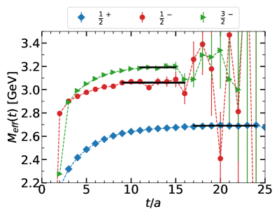
Figure 8: Effective mass plots for $\Lambda_{c}\left(\frac{1}{2}^{+}\right)$ (blue diamond), $\Lambda_{c}\left(\frac{1}{2}^{-}\right)$ (red circle) and $\Lambda_{c}\left(\frac{3}{2}^{-}\right)$ (green triangle).

VI.2 $cD$ NBS wave function and the pre-potential

In order to extract the NBS wave function, we begin with the definition of the $cD$ four-point correlator $G_{cD,\alpha\beta}(\bm{r},t)$ given by

$$G_{cD,\alpha\beta}(\bm{r},t)$$

$$\equiv \frac{1}{V}\sum_{\bm{\Delta}}\left\langle 0\left|T\left[D_{a}(\bm{r}+\bm{\Delta},t_{{\rm sink}})c_{a,\alpha}(\bm{\Delta},t_{{\rm sink}})\cdot\overline{\mathcal{B}}_{\beta}(t_{{\rm src}})\right]\right|0\right\rangle,$$

where $a$ denotes the color index. We focus on the degenerated components $(\alpha,\beta)=(1,1),(2,2)$ which represent the positive-to-positive parity propagation, and omit the spinor indices hereafter. The degenerated components are later averaged over to reduce the statistical error.

As demonstrated for the $c\bar{c}$ four-point correlator in subsectionV.2, the $cD$ four-point correlator is spectrally decomposed as

$$G_{cD}(\bm{r},t)=\sum_{n}\psi^{(n)}_{cD}(\bm{r})a_{n}e^{-M_{n}t}$$ (43)

where $\psi^{(n)}_{cD}(\bm{r})$ , $a_{n}=\langle n|\overline{\mathcal{B}}(0)|0\rangle$, and $M_{n}$ denote the NBS wave function, the overlap, and the mass of the $n$-th excited state, respectively. In the large time region, the excited states are suppressed and the ground state $\Lambda_{c}(\frac{1}{2}^{+})$ becomes dominant. For this reason, we denote $\psi^{(0)}_{cD}(\bm{r},t)$ as $\psi_{\Lambda_{c}}(\bm{r},t)$. To proceed, we project the wave function to the S-wave by the $A_{1}$ projection Eq. (29).

Fig.9 shows the $cD$ NBS wave functions in several representative time slices. As in the case of $c\bar{c}$, we focus on the wave function at $t=17$ here as the representative one from now on.

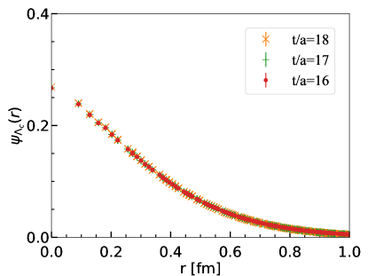
Figure 9: $cD$ NBS functions for the $\Lambda_{c}(\frac{1}{2}^{+})$ state at $16\leq t/a\leq 18$. Each wave function is normalized as $\sum_{r\in V}\bm{r}^{2}\psi_{\Lambda_{c}}^{2}(\bm{r})=1$.

Note that the $cD$ NBS wave function is spatially extensive and experiences reflection at the boundary. Then, the wave function is deformed from the S-wave especially in the long range region Aoki et al. (2005). Our observation is corroborated by the growing systematic uncertainty at $r/a\simeq 10$ ($r\sim 0.91$ fm) due to the reflection. In order to avoid this undesirable effect, we limit the range to $r/a\leq 9$ ($r\lessapprox 0.82$ fm).

VI.3 Eigen value problem and the Diquark mass

We construct the $cD$ pre-potential in the same way as for the $c\bar{c}$ pre-potential in Section V. Then, we first fit to ALL in the range $1\leq r/a\leq 9$ ($0.1\lessapprox r\lessapprox 0.82$ fm) to the Cornell function $f(r)=-A/r+Br+C$ without the log term. As the left panel of Fig.10 shows, most of the data points lie close to the curve. Thus this fitting is adequate. Note that the fit yields relatively large chi-square of $\chi^{2}/N_{{\rm d.o.f}}\simeq 23$ as in the case of $c\bar{c}$ system due to the singularity near origin and the direction dependence. Next, we fit the data points for the three series separately as before by setting the fit range appropriately to $3\leq r/a\leq 9$ ($0.27\lessapprox r\lessapprox 0.82$ fm). The fit is adequate as shown in the right panel of Fig.10, yielding $\chi^{2}/N_{{\rm d.o.f}}$; $\chi^{2}/N_{{\rm d.o.f}}\simeq 2.7$, $0.47$ for $0.24$ for Series I, II and III , respectively.

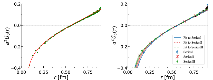
Figure 10: Cornell function fit to the $cD$ pre-potential (black dots). Left panel shows the fit to ALL and right shows the fit to Series I,II and III .

Substituting the fit result into Eq. (37), we solve the eigenvalue problem for the S-wave and the P-wave. The left panel of Fig.11 shows the solution for ALL whereas the right panel shows the numerical solutions of the three series. In contrast to the $c\bar{c}$ system, the fit to ALL happens to reproduce the NBS wave function very well. We see in the right panel of Fig.11 that the numerical result for the series and the LQCD data roughly agree. The wave functions of ALL and III almost coincide. As was discussed in subsection.V.4 in the context of the spherical harmonic expansion, Series I is known to be the farthest from the S-wave. Series III reproduces the NBS wave function seemingly the best. The values of the RSS are $\sqrt{\delta_{\rm RSS}}\simeq 1\cdot 10^{-2}$, $8\cdot 10^{-2}$, $4\cdot 10^{-2}$ and $9\cdot 10^{-3}$ for ALL, Series I, Series II and Series III , respectively. The P-wave, on the other hand, is weakly affected by the direction dependence near origin, and thus the solutions for the series are indistinguishable.

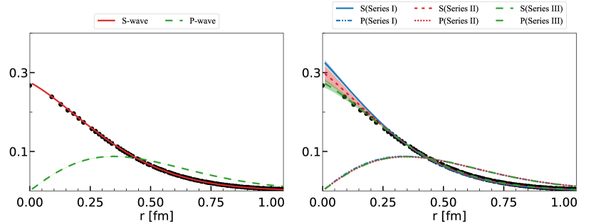
Figure 11: Numerical solution from (left) ALL and (right) Series I, II and III . The LQCD data of the NBS wave function (black circles) is shown for comparison.

The reduced mass $\mu_{cD}$ is obtained by Eq. (20) using $\tilde{E}_{\rm PW}$ and the $\Lambda_{c}$ mass obtained in subsection VI.1. Then, the diquark mass is obtained by substituting the charm quark mass $m_{c}$ into Eq. (21). Table 8 summarizes the diquark mass obtained from each series. The value of the diquark mass is roughly consistent with naive expectations from the constituent quark picture, i.e. the $\rho$ meson mass $M_{\rho}=1.098(5)$ GeV and twice the constituent mass $\frac{2}{3}M_{N}=1.049(12)$ GeV. We see in the table that the diquark mass obtained from ALL, Series II and Series III are close to each other while that from Series I is larger than the others. This becomes more evident when we plot the mass as shown in Fig.12. For the sake of consistency with the $c\bar{c}$ system, let us use the diquark mass from ALL hereafter for necessary conversions.

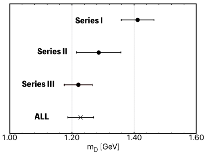
Figure 12: Direction dependence of the diquark mass.

Table 8: Summary of the diquark quark mass.

directions	ALL	Series I	Series II	Series III
$m_{D}$ [GeV]	1.273 (44)	1.470 (57)	1.335 (77)	1.264 (49)

Now, the $cD$ potential is given by $U_{0}(r)=\frac{1}{2\mu_{cD}}\tilde{U}_{0}(r)+E_{\Lambda_{c}(\frac{1}{2}^{+})}$. Table 9 shows the coefficients of the Cornell function fit to the $cD$ potential. We see that the direction dependence of the Coulomb coefficient is large compared to that of the string tension. This is because the Coulomb term is determined in the short range region where the discretization errors are large. It should also be noted that the string tension has some direction dependence as Table 9 shows. One reason for this is that the string tension is affected by the direction dependence of the Coulomb coefficient because the region where the linear part is overwhelmingly dominant is not reached. Moreover, the reflected waves cause systematic errors to the linear part of the $cD$ potential, making it difficult to reach the desired asymptotic region. It is necessary to calculate with a larger lattice as well as to obtain information from excited state wave functions with greater spatial extents. In this way, the string tension may be determined with higher precision.

Table 9: Summary of the Cornell function fit to the $cD$ potential.

direction	$A$ [GeV$\cdot$fm]	$B$ [GeV/fm]	$C$ [GeV]
ALL	0.065(2)	1.315(24)	-0.889(34)
Series I	0.107(7)	1.157(53)	-0.728(52)
Series II	0.089(16)	1.195(78)	-0.778(82)
Series III	0.066(11)	1.300(71)	-0.876(68)

VII Comparing $cD$ potential and $c\bar{c}$ potential

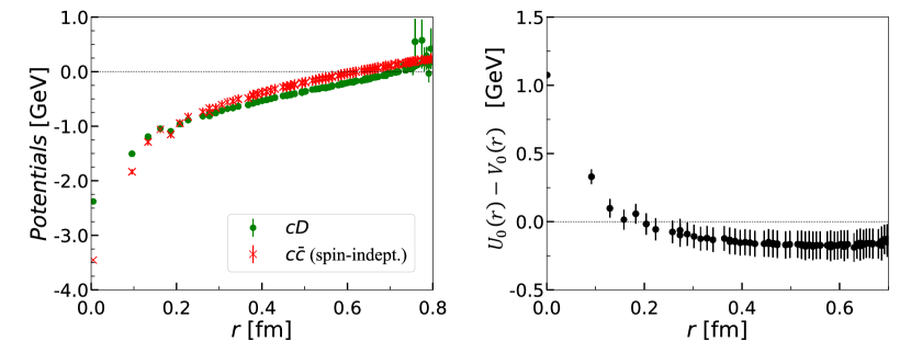
Figure 13: (left) $cD$ potential $U_{0}(r)$ compared with the spin-independent part of the $c\bar{c}$ potential $V_{0}(r)$. (right) Difference between $U_{0}(r)$ and $V_{0}(r)$.

Fig.13 compares the $cD$ potential $U_{0}(r)$ and the spin-independent part of the $c\bar{c}$ potential $V_{0}(r)$. It shows that their data points are almost parallel in the region $r\geq 0.4$ fm. The difference between the two sets is essentially a constant as shown on a magnified scale in the right panel of Fig.13. Thus the linearly rising part of $U_{0}(r)$ and $V_{0}(r)$ cancel each other. This behavior can be understood as follows. First, the anti-charm quark and the diquark are in the same color representation $\overline{\bm{3}}$. Thus the $c\bar{c}$ potential and the $cD$ potential are identical in principle if it were not for the internal structures of the diquark. Though the diquark is not point-like Alexandrou et al. (2006), diquark structure is less important at long distances and the color representation governs the potential. Indeed, it is reported in the earlier LQCD works Takahashi et al. (2001a); Sakumichi and Suganuma (2015); Takahashi et al. (2001b) that the diquark limit of the static three quark potential (QQQ potential) and the static $Q\bar{Q}$ potential coincide.

At short distances, on the other hand, the magnitude of the Coulomb attraction of the $cD$ potential is smaller than that of the $c\bar{c}$ potential. This mitigation of the Coulomb attraction is most likely caused by the internal structure of the diquark, namely its spatial extent. In fact, the refrences Jido and Sakashita (2016); Kumakawa and Jido (2017) shows that the Coulomb attraction is suppressed when the diquark has a finite spatial extent. Note that the diquark limit in the QQQ system realizes a point-like diquark. Thus, the Coulomb attraction of the QQQ potential in the diquark limit is not weakened by the finite size effect of the diquark. Hence, it stands to reason that the attraction of our $cD$ potential is different from the diquark limit of the QQQ potential.

Fig.14 compares the Cornell function fit to $U_{0}(r)$ and $V_{0}(r)$. Table 10 summarizes the fitting parameters where we immediately see that the values of the string tension are roughly the same as expected from Fig.13.

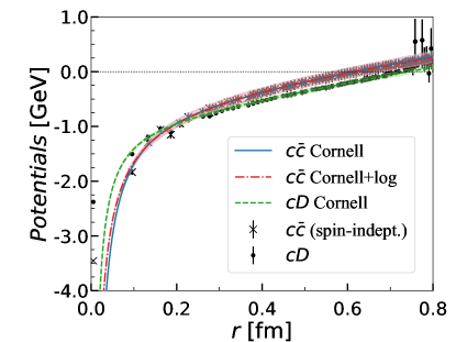
Figure 14: Cornell function fit to the $cD$ potential and to the spin-independent part of the $c\bar{c}$ potential. We also show the Cornell+log type function fit to the $c\bar{c}$ potential for a reference.

Table 10: Comparison of the the $cD$ potential and the $c\bar{c}$ potential fit to the Cornell function for ALL in the range $1\leq r/a\leq 9$.

	$A$ [GeV$\cdot$fm]	$B$ [GeV/fm]	C [GeV]
$cD$	0.065(2)	1.315(24)	-0.889(34)
$c\bar{c}$	0.124(3)	1.247(24)	-0.576(80)

VIII Conclusions

We have reported on the novel and consistent method which we developed to evaluate the charm-diquark interaction potential, the diquark mass and the charm quark mass. Specifically, we applied our method by considering the $\Lambda_{c}$ baryon as a bound state of a charm quark and a scalar-diquark. The diquark mass obtained from our method was $m_{D}=1.273(44)$ GeV which does not contradict the conventional estimates; our diquark mass is slightly above the $\rho$ meson mass $m_{\rho}=1.098(5)$ GeV and twice the constituent quark mass $2m_{N}/3=1.049(12)$ GeV. When applied to the charmonium, our method yielded $m_{c}=1.686(44)$ GeV for the charm quark mass. This is $\sim 250$ MeV smaller than the value $m_{c}=1.933(17)$ GeV obtained by the Kawanai-Sasaki method. Our charm-diquark potential is given by the well-known Cornell potential where the Coulomb attraction was found considerably weaker than that of the $c\bar{c}$ potential. The weakening is most likely due to the structure of the diquark, namely its spatial extent. These quantities allow us to construct a QCD-based quark-diquark model that can be used to investigate the hadron levels and structures.

In this work, we observed that there are three major systematic uncertainties in our $cD$ potential and $c\bar{c}$ potential. One is in the short range region cased by the discretized Laplacian, and the second is the discretized lattice actions and the gauge fixing. The last is from the reflection from the boundaries. The first two errors may be reduced by calculating with finer lattice and with improved actions and gauge fixing procedure. Lattice setups with larger spatial extent is desirable for the third.

The quark-diquark potential and diquark mass in this study are obtained from lattice setup with $m_{\pi}\simeq 700$ MeV. However, this is not the value at the physical point where the pion mass is $m_{\pi}\simeq 140$ MeV. In order to construct a diquark model which outputs observables that can be compared with experimental results, it is necessary to calculate the quark-diquark potential and the diquark mass at the physical point. This is achieved by extrapolating to the physical point. For example, we may calculate using available PACS-CS configurations corresponding to $m_{\pi}\simeq 540$ MeV, $m_{\pi}\simeq 410$ MeV, etc. and extrapolate the obtained results to the physical point. Physical observables such as levels of Baryon and exotic candidates calculated using the diquark model are comparable to experimental results.

Moreover, it is presumed that pseudo-scalar, vector and axial-vector diquarks may play crucial roles in a general context of hadron physics. Straightforward extension of our method to the above mentioned diquarks seems to be an interesting step to pursue.

IX Acknowledgement

The author thanks N. Ishii, A. Hosaka, M. Koma, A. Nakamura, Tm. Doi and K. Sasaki for fruitful discussions. The Lattice QCD calculation has been carried out by using the supercomputer OCTOPUS at Cyber Media Center of Osaka University under the support of Research Center for Nuclear Physics of Osaka University. We also thank PACS-CS Collaboration and ILDG/JLDG for providing us with the 2+1 flavor QCD gauge configurations  Aoki et al. (2009); Beckett et al. (2011); ILD ; JLD . The lattice QCD code is partly based on Bridge++ Bri . This research is supported by MEXT as “Program for Promoting Researches on the Supercomputer Fugaku” (Simulation for basic science: from fundamental laws of particles to creation of nuclei) and JICFuS and by JSPS KAKENHI Grant Number JP21K03535.

Appendix A $m_{q}$ determination using the spin triplet sector

To obtain the charm quark mass using the spin triplet sector, we start with replacing $\tilde{V}^{{\rm fit}}_{{\rm PS}}(r)$ in the Schrödinger equation Eq. (37) by $\widetilde{V}^{{\rm fit}}_{V}(r)=\widetilde{V}^{\rm fit}_{0}(r)+\frac{1}{4}\widetilde{V}^{\rm fit}_{\sigma}(r)$.

We use the pre-potential fit to Series II in Section V. Then the spin-orbit averaged P-wave excitation pre-energy is obtained by incorporating the centrifugal potential as was demonstrated in Eq. (II.2.2) for the spin singlet sector. Fig.15 compares the V channel numerical solutions to the NBS wave function where we find a good agreement.

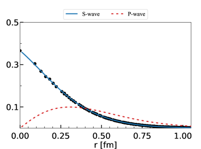
Figure 15: Numerical solutions for S-wave (S) and P-wave (P). Black circles denote the NBS wave function data.

Next, we replace $M_{{\rm T}}-M_{{\rm PS}}$ by $2M_{{\rm AV}}-M_{{\rm S}}-M_{{\rm V}}$ in Eq. (12) where we have neglected the small contribution from the tensor interaction. Then, by substituting the P-wave pre-excitation energy into Eq. (12), we get charm quark mass $1.604(76)$ GeV, which is consistent with that from the singlet sector within the statistical error. Note that for better precision, the energy level of $2^{++}$ state ($\chi_{c2}$ meson) needs to be taken into account to offset the effect of the tensor interaction.

Appendix B Cubic group transformations

The cubic group has 48 elements, each being products of three $\frac{\pi}{2}$-rotations about $x$, $y$ and $z$ axes and the parity transformation. The elements are representable by the parity-inversion and the order 4 sub-group matrices $C_{x}$, $C_{y}$ and $C_{z}$ given by

$$\begin{array}[]{lll}C_{x}=\begin{pmatrix}&\ 1&&\ 0&&\ 0&\\ &\ 0&&\ 0&&-1&\\ &\ 0&&\ 1&&\ 0&\end{pmatrix},C_{y}=\begin{pmatrix}&\ 0&&\ 0&&\ 1&\\ &\ 0&&\ 1&&\ 0&\\ &-1&&\ 0&&\ 0&\end{pmatrix},C_{z}=\begin{pmatrix}&\ 0&&-1&&\ 0&\\ &\ 1&&\ 0&&\ 0&\\ &\ 0&&\ 0&&\ 1&\end{pmatrix}\end{array}.$$ (44)

Table 11 summarizes the 24 proper rotations. Combining these and the parity-inversion, we get 48 elements of $O_{h}$.

Table 11: 24 matrices of proper rotation and the order of each element.

Order	Matrices
1	$C_{0}\equiv\rm{unity}$
4	$\begin{array}[]{cccc}C_{x},&C_{y},&C_{z}&\\ C_{x}^{-1},&C_{y}^{-1},&C_{z}^{-1},&\end{array}$
3	$\begin{array}[]{ccccc}C_{x}C_{y},&C_{z}C_{y},&C_{x}C_{z},&C_{y}C_{x}&\\ (C_{x}C_{y})^{2},&(C_{y}C_{x})^{2},&(C_{z}C_{y})^{2},&(C_{x}C_{z})^{2}&\end{array}$
2	$C_{x}^{2},C_{y}^{2},C_{z}^{2}$
2	$\begin{array}[]{cccc}C_{x}C_{y}C_{z},&C_{y}C_{z}C_{x},&C_{z}C_{x}C_{y}\\ C_{x}^{-1}C_{y}^{-1}C_{z},&C_{y}^{-1}C_{z}^{-1}C_{x},&C_{z}^{-1}C_{x}^{-1}C_{y}\end{array}$

References

- Gell-Mann (1964) M. Gell-Mann, Phys. Lett. 8, 214 (1964).
- WILCZEK (2005) F. WILCZEK, From Fields to Strings: Circumnavigating Theoretical Physics , 77â93 (2005).
- Jaffe (2005) R. Jaffe, Physics Reports 409, 1 (2005).
- Santopinto (2005) E. Santopinto, Phys. Rev. C 72, 022201(R) (2005).
- Lichtenberg et al. (1968) D. B. Lichtenberg, L. J. Tassie, and P. J. Keleman, Phys. Rev. 167, 1535 (1968).
- Lichtenberg et al. (1982) D. B. Lichtenberg, W. Namgung, E. Predazzi, and J. G. Wills, Phys. Rev. Lett. 48, 1653 (1982).
- Galatà and Santopinto (2012) G. Galatà and E. Santopinto, Phys. Rev. C 86, 045202 (2012).
- Oettel et al. (1998) M. Oettel, G. Hellstern, R. Alkofer, and H. Reinhardt, Phys. Rev. C 58, 2459 (1998).
- Segovia et al. (2015) J. Segovia, C. D. Roberts, and S. M. Schmidt, Physics Letters B 750, 100 (2015).
- Jido and Sakashita (2016) D. Jido and M. Sakashita, Progress of Theoretical and Experimental Physics 2016, 10.1093/ptep/ptw113 (2016), 083D02.
- Kumakawa and Jido (2017) K. Kumakawa and D. Jido, Progress of Theoretical and Experimental Physics 2017, 10.1093/ptep/ptx155 (2017), 123D01.
- Chen et al. (2018) C. Chen, B. El-Bennich, C. D. Roberts, S. M. Schmidt, J. Segovia, and S. Wan, Phys. Rev. D 97, 034016 (2018).
- Maiani et al. (2015) L. Maiani, A. Polosa, and V. Riquer, Physics Letters B 749, 289 (2015).
- Giannuzzi (2019) F. Giannuzzi, Physical Review D 99, 094006 (2019).
- Giron and Lebed (2020) J. F. Giron and R. F. Lebed, Phys. Rev. D 102, 074003 (2020).
- Johnson and Thorn (1976) K. Johnson and C. B. Thorn, Phys. Rev. D 13, 1934 (1976).
- Anselmino et al. (1993) M. Anselmino, E. Predazzi, S. Ekelin, S. Fredriksson, and D. B. Lichtenberg, Rev. Mod. Phys. 65, 1199 (1993).
- Hess et al. (1998) M. Hess, F. Karsch, E. Laermann, and I. Wetzorke, Phys. Rev. D 58, 111502(R) (1998).
- Bi et al. (2016) Y. Bi, H. Cai, Y. Chen, M. Gong, Z. Liu, H.-X. Qiao, and Y.-B. Yang, Chinese Physics C 40, 073106 (2016).
- Alexandrou et al. (2006) C. Alexandrou, P. de Forcrand, and B. Lucini, Phys. Rev. Lett. 97, 222002 (2006).
- Francis et al. (2021) A. Francis, P. de Forcrand, R. Lewis, and K. Maltman, Diquark properties from full qcd lattice simulations (2021), arXiv:2106.09080 [hep-lat] .
- Aoki and Doi (2020) S. Aoki and T. Doi, Frontiers in Physics 8, 307 (2020).
- Ishii et al. (2007) N. Ishii, S. Aoki, and T. Hatsuda, Phys. Rev. Lett. 99, 022001 (2007).
- Iritani et al. (2019) T. Iritani, S. Aoki, T. Doi, S. Gongyo, T. Hatsuda, Y. Ikeda, T. Inoue, N. Ishii, H. Nemura, and K. Sasaki (HAL QCD Collaboration), Phys. Rev. D 99, 014514 (2019).
- Ikeda and Iida (2012) Y. Ikeda and H. Iida, Progress of Theoretical Physics 128, 941 (2012).
- Bali et al. (2005) G. S. Bali, H. Neff, T. Düssel, T. Lippert, and K. Schilling (SESAM Collaboration), Phys. Rev. D 71, 114513 (2005).
- Bali (2001) G. S. Bali, Phys. Rept. 343, 1 (2001), hep-ph/0001312 .
- Eichten et al. (1975) E. Eichten, K. Gottfried, T. Kinoshita, J. Kogut, K. D. Lane, and T. M. Yan, Phys. Rev. Lett. 34, 369 (1975).
- Kawanai and Sasaki (2011) T. Kawanai and S. Sasaki, Phys. Rev. Lett. 107, 091601 (2011), 1102.3246 .
- Kawanai and Sasaki (2015) T. Kawanai and S. Sasaki, Phys. Rev. D 92, 094503 (2015).
- Nochi et al. (2016) K. Nochi, T. Kawanai, and S. Sasaki, Phys. Rev. D 94, 114514 (2016).
- Koma and Koma (2013) Y. Koma and M. Koma, Few-Body Systems 54 (2013).
- Sugiura et al. (2016) T. Sugiura, K. Murano, N. Ishii, and M. Oka, Proceedings, 34th Lattice 2016: Southampton, UK, July 24-30, 2016, PoS LATTICE2016, 122 (2016), 1703.09936 .
- Aoki et al. (2009) S. Aoki, K.-I. Ishikawa, N. Ishizuka, T. Izubuchi, D. Kadoh, K. Kanaya, Y. Kuramashi, Y. Namekawa, M. Okawa, Y. Taniguchi, A. Ukawa, N. Ukita, and T. Yoshié (PACS-CS Collaboration), Phys. Rev. D 79, 034503 (2009).
- Iwasaki (2011) Y. Iwasaki, unpublished (2011), arXiv:1111.7054 [hep-lat] .
- Aoki et al. (2006) S. Aoki, M. Fukugita, S. Hashimoto, K.-I. Ishikawa, N. Ishizuka, Y. Iwasaki, et al. (CP-PACS and JLQCD Collaborations), Phys. Rev. D 73, 034501 (2006).
- Aoki et al. (2003) S. Aoki et al., Progress of Theoretical Physics 109, 383 (2003).
- Namekawa et al. (2013) Y. Namekawa, S. Aoki, K.-I. Ishikawa, N. Ishizuka, K. Kanaya, Y. Kuramashi, M. Okawa, Y. Taniguchi, A. Ukawa, N. Ukita, and T. Yoshié (PACS-CS Collaboration), Phys. Rev. D 87, 094512 (2013).
- Gattringer and Lang (2009) C. Gattringer and C. Lang, Quantum chromodynamics on the lattice: an introductory presentation, Vol. 788 (Springer Science & Business Media, 2009).
- Lüscher (1991) M. Lüscher, Nuclear Physics B 354, 531 (1991).
- Aoki et al. (2005) S. Aoki, M. Fukugita, K.-I. Ishikawa, N. Ishizuka, Y. Iwasaki, K. Kanaya, T. Kaneko, Y. Kuramashi, M. Okawa, A. Ukawa, T. Yamazaki, and T. Yoshié (CP-PACS Collaboration), Phys. Rev. D 71, 094504 (2005).
- Sasaki and Ishizuka (2008) K. Sasaki and N. Ishizuka, Phys. Rev. D 78, 014511 (2008).
- Koma et al. (2006) Y. Koma, M. Koma, and H. Wittig, Phys. Rev. Lett. 97, 122003 (2006).
- Pérez-Nadal and Soto (2009) G. Pérez-Nadal and J. Soto, Phys. Rev. D 79, 114002 (2009).
- Colbert and Miller (1992) D. T. Colbert and W. H. Miller, The Journal of Chemical Physics 96, 1982 (1992).
- Light and Walker (1976) J. C. Light and R. B. Walker, The Journal of Chemical Physics 65, 4272 (1976).
- Zanotti et al. (2003a) J. M. Zanotti, D. B. Leinweber, A. G. Williams, J. B. Zhang, W. Melnitchouk, and S. Choe (CSSM Lattice Collaboration), Phys. Rev. D 68, 054506 (2003a).
- Benmerrouche et al. (1989) M. Benmerrouche, R. M. Davidson, and N. C. Mukhopadhyay, Phys. Rev. C 39, 2339 (1989).
- Alexandrou et al. (2014) C. Alexandrou, V. Drach, K. Jansen, C. Kallidonis, and G. Koutsou, Phys. Rev. D 90, 074501 (2014).
- Zanotti et al. (2003b) J. Zanotti, S. Choe, D. Leinweber, W. Melnitchouk, A. Williams, and J. Zhang, Nucl. Phys. B Proc. Suppl. 119, 299 (2003b).
- Bahtiyar et al. (2020) H. Bahtiyar, K. U. Can, G. Erkol, P. Gubler, M. Oka, and T. T. Takahashi (TRJQCD Collaboration), Phys. Rev. D 102, 054513 (2020).
- Takahashi et al. (2001a) T. T. Takahashi, H. Matsufuru, Y. Nemoto, and H. Suganuma, Phys. Rev. Lett. 86, 18 (2001a).
- Sakumichi and Suganuma (2015) N. Sakumichi and H. Suganuma, Phys. Rev. D 92, 034511 (2015).
- Takahashi et al. (2001b) T. T. Takahashi, H. Matsufuru, Y. Nemoto, and H. Suganuma, Phys. Rev. Lett. 86, 18 (2001b).
- Beckett et al. (2011) M. G. Beckett, P. Coddington, B. Joó, C. M. Maynard, D. Pleiter, O. Tatebe, and T. Yoshie, Computer Physics Communications 182, 1208 (2011).
- (56) International Lattice Data Grid (ILDG), http://www.lqcd.org/ildg.
- (57) Japan Lattice Data Grid (JLDG), http://www.jldg.org.
- (58) Lattice QCD code Bridge++, http://bridge.kek.jp/Lattice-code/.