Towards combinatorial invariance for Kazhdan-Lusztig polynomials
Abstract.
Kazhdan-Lusztig polynomials are important and mysterious objects in representation theory. Here we present a new formula for their computation for symmetric groups based on the Bruhat graph. Our approach suggests a solution to the combinatorial invariance conjecture for symmetric groups, a well-known conjecture formulated by Lusztig and Dyer in the 1980s.
1. Introduction
Kazhdan-Lusztig polynomials are important polynomials associated to pairs of elements in Coxeter groups. They appear throughout representation theory and related fields. Lusztig (ca. 1983) and Dyer (1987) independently conjectured that Kazhdan-Lusztig polynomials depend only on the poset of elements between and in Bruhat order. This is a fascinating conjecture. For example, it suggests that Kazhdan-Lusztig polynomials are providing subtle invariants of Bruhat order. This conjecture is known in several special cases ([Dye87, Bre04, Inc06, BCM06, Pat21, BLP21], see [Bre04] for an overview).
In this work we prove a new formula Kazhdan-Lusztig polynomials for symmetric groups. Our formula was discovered whilst trying to understand certain machine learning models trained to predict Kazhdan-Lusztig polynomials from Bruhat graphs (see [DVB+]). The new formula suggests an approach to the combinatorial invariance conjecture for symmetric groups.
Traditionally, Kazhdan-Lusztig polynomials are computed inductively based on the length. This means that in order to compute one might need to know where lies anywhere in . Our new formula allows inductive calculation using only polynomials where belong to the Bruhat interval —thus it “stays in the Bruhat interval”. Roughly speaking, we compute Kazhdan-Lusztig polynomials via induction over the rank of the symmetric group, rather than the length of a permutation.
As our new formula uses only information present in the Bruhat interval and thus might be useful for approaching the combinatorial invariance conjecture. However, the formula requires the knowledge of the intersection of with a coset , which is not combinatorially invariant information. It is not difficult to see that the intersection
forms a sub-interval . We observe that the embedding has remarkable properties: the edges connecting any node to a node possess a lattice-like quality which we call a hypercube cluster.
Abstracting the notion of hypercube cluster leads to the general notion of hypercube decomposition of which our sub-interval is an example. Hypercube decompositions appear to provide a nice general way of understanding Bruhat intervals in symmetric groups. We expect them to play a role in the solutions of other problems. In general, there may be many more hypercube decompositions than come from intersections with cosets of . Remarkably, our formula appears to give the right answer for any hypercube decomposition. We cojecture that this is always the case. We have checked our conjecture on all Bruhat intervals up to (over a million Bruhat intervals, and many more hypercube decompositions!). Our conjecture implies the combinatorial invariance conjecture in more precise form.
1.1. Structure of this paper
We begin in §2 with an overview of Kazhdan-Lusztig polynomials and the combinatorial invariance conjecture. This is introductory, and can be skipped over by an experienced reader. In §3 we introduce hypercube clusters, and state our formula and conjecture. This section is purely combinatorial. In §4 and §5 we prove our formula; here geometric machinery (Schubert varieties, intersection cohomology, torus actions, weights …) is needed. In §6 we outline a route to a proof of our conjecture in general, and explain that our conjecture would follow from the purity of a certain cohomology group, or the surjectivity of restriction map map in cohomology.
1.2. Acknowledgements
We are grateful to Erez Lapid, Matthew Dyer, Peter Fiebig, Leonardo Patimo and Joel Kamnitzer for useful discussions and/or correspondence. We are particularly grateful to Anthony Henderson for patiently listening to our incomplete explanations, and numerous helpful suggestions.
2. Kazhdan-Lusztig polynomials and combinatorial invariance
In this background section, we give some background on Coxeter groups, Bruhat graphs, Kazhdan-Lusztig polynomials and the combinatorial invariance conjecture. Excellent references for the following include [Hum90, Bre04, BB05, Soe97, EMTW20].
2.1. Coxeter groups and Kazhdan-Lusztig polynomials
Coxeter groups are an important class of groups, which arose out of H. S. M. Coxeter’s study of finite reflection groups in the 1930s. They are characterised by a presentation via generators and relations. In this presentation the generating set are called the simple reflections. An important example of a Coxeter group is the symmetric group consisting of all permutations of , with simple reflections consisting of the set of adjacent transpositions.
In a seminal paper [KL79], Kazhdan and Lusztig associated to any pair of elements in a Coxeter group a polynomial with integer coefficients
known as the Kazhdan-Lusztig polynomial. All that we say here concerning their definition is that it is highly inductive; one works one’s way “out” in the group, starting at the identity and applying generators from . At each step in the calculation one might need any of the previously computed polynomials. Thus, they are rather cumbersome to calculate by hand, but it is not difficult to compute billions of them on a computer with enough memory. (This is useful for machine learning, as one often needs access to large data sets.)111The reader who wants to get a feeling for Kazhdan-Lusztig polynomials is encouraged to experiment with Joel Gibson’s LieVis software. For example, Kazhdan-Lusztig for an affine Weyl group of type are computed live here.
2.2. The Bruhat graph
To any Coxeter group one may associate its Bruhat graph. For the symmetric group, this is the graph with vertices corresponding to all elements of , and an edge joining and if and only if they differ by multiplication by a transposition. (In other words, and are connected in the Bruhat graph if they agree on all but two elements of .) Below, we will denote the transposition that exchanges and by . The transpositions are precisely the conjugates of the simple reflections in .
The symmetric group has a natural length function given by the number of inversions:
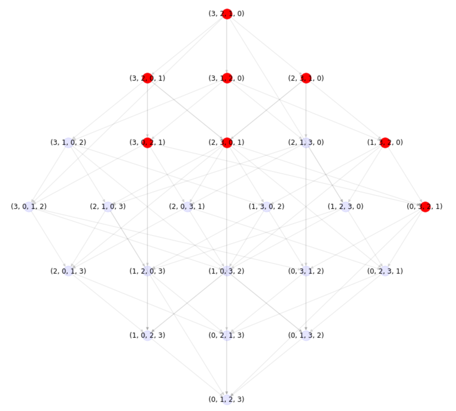
We regard the length function as giving us a notion of “height” on the Bruhat graph. This allows us to orient the edges of the Bruhat graph via decreasing length. Figures 1 and 2 give pictures of the Bruhat graph for and .222Throughout this paper we use string notation for permutations. Thus (or often simply ) denotes the permutation of and that sends , , and .
2.3. Bruhat order
The Bruhat graph allows us to define the Bruhat order, which is a partial order on . It is defined as follows:
| (1) |
(We include paths of length zero, so always holds.) For example, in the symmetric group the minimal element is always the identity permutation, and the maximal element is the permutation which interchanges and , and etc.
The Bruhat order is remarkably complex, and it has long been suspected that Kazhdan-Lusztig polynomials reflect subtle properties of the Bruhat order. An elementary manifestation of this phenomenon (easy to prove) is that:
Less elementary connections tend to involve the interval consisting of the full subgraph of the Bruhat graph between and . (That is, this consists of all edges and vertices which may be reached from on the way to , whilst progressing downwards.) For example, a much less obvious fact [Car94, Dye93] is that
(It is easy to see that the full Bruhat graph is regular, and in particular .)
2.4. First examples
In all proper intervals are isomorphic to the following posets333poset = partially ordered set (as the reader may check easily, using Figure 1):
All these graphs are regular (after forgetting edge orientations), and thus all Kazhdan-Lusztig polynomials are .
In , almost all intervals are regular, and hence almost all Kazhdan-Lusztig polynomials are 1. There are four intervals which are not regular. Here we depict two intervals which are not: those between and , and between and :
In both cases, the interval is isomorphic to the following directed graph, known as the “4 crown”:
| (3) |
In both these cases the Kazhdan-Lusztig polynomials are equal:
| (4) |
2.5. The combinatorial invariance conjecture
The following conjecture, formulated independently by Lusztig and Dyer in the 1980s, was a major motivation for the current work:
Conjecture 2.1.
The Kazhdan-Lusztig polynomial depends only on the isomorphism type of Bruhat graph of the interval .
For example, given only the ordered graph (3) (and not the labelling of its vertices) we should be able to predict the Kazhdan-Lusztig polynomial . The fact that (3) occurs in two different ways in the Bruhat graph of with equal Kazhdan-Lusztig polynomials, can be seen as an instance of this conjecture. Figures 3 and 4 shows two more examples of the assignment of Kazhdan-Lusztig polynomial to Bruhat intervals.
Remark 2.2.
The combinatorial invariance conjecture is a central conjecture in the study of Bruhat intervals. The reader is referred to [Bre04] for more detail on known cases (see also [Dye87, Bre04, Inc06, Pat21, BLP21]). We do not discuss the various partial results towards the conjecture here, except to mention that it is known to hold for intervals starting at the identity [BCM06].
3. The new formula
In this section we describe our new formula. Before going into detail, let us give a rough idea of what the formula looks like. Recall that our goal is to compute the Kazhdan-Lusztig polynomial starting from the Bruhat graph. By induction, we can assume that we can do this for any smaller graph. In particular, we can assume that all intermediate polynomials are known, for all with .
Our formula depends on the choice of an auxiliary structure on our graph, called a hypercube decomposition. Such a decomposition amounts to the choice of a subinterval satisfying certain concrete combinatorial conditions. (The reader is encouraged to skip ahead a few pages to Figure 6, where a typical hypercube decomposition is illustrated.) There always exists at least one hypercube decomposition, but in general there will be many. Any choice of hypercube decomposition determines two polynomials in , the inductive piece and hypercube piece. Our formula is:
| (5) |
The left hand side is the -derivative of the Kazhdan-Lusztig polynomial, from which the Kazhdan-Lusztig polynomial can be recovered. The calculation of the inductive piece (resp. hypercube piece) uses only the part of the graph which lies (resp. does not lie) in . (Again, the reader is encouraged to glance at Figure 6. The nodes necessary for the computation of the hypercube and inductive piece are in blue (resp. red).)
3.1. The -derivative of Kazhdan-Lusztig polynomials
We now introduce a new polynomial, whose knowledge is equivalent to knowledge of the Kazhdan-Lusztig polynomial, but which is easier to handle. Define
(One checks easily that the denominator always divides the numerator, so is always an integer valued polynomial.) We refer to as the -derivative of the Kazhdan-Lusztig polynomial.444In the related theory of Kazhdan-Lusztig-Stanley polynomials, this polynomial is often called the “-polynomial”. Defining properties of Kazhdan-Luztig polynomials555more precisely, the fact that their degree is bounded above by ensure that determines .
Example 3.1.
We give three examples of Kazhdan-Lusztig polynomials, and their corresponding -derivatives:
-
(1)
, , , .
-
(2)
, , , .
-
(3)
, , , .
(We leave it up to the reader to determine the meaning of the box diagrams, as well as how to recover the Kazhdan-Lusztig polynomial from them.)
3.2. Hypercube clusters
We work in the setting of directed acyclic graphs. Any such graph is a poset in natural way, where we declare if there exists a directed path from to .
For any finite set , the -hypercube is the directed acyclic graph with:
-
(1)
vertices consisting of subsets of ;
-
(2)
an edge if is obtained from by removing one element.
Example 3.2.
-hypercubes for , and :
Now suppose given a directed acyclic graph (in our applications will be a Bruhat graph) and a node . We say that a subset of edges with target spans a hypercube if there exists a unique embedding (i.e. injection) of directed graphs
sending the edge in to , for all edges in . If spans a hypercube, its crown is .
Example 3.3.
Consider the following directed graph (isomorphic to the Bruhat graph of ):
In the following we show some pairs of edges with common target with a colour. The pairs of red marked edges do not span hypercubes, whereas the blue edges do:
It should be clear that the first pair of red edges do not span a hypercube. In the second example, the issue is that there is not a unique way to map in a hypercube, with these specified base vertices.
We now come to a key definition. Suppose that is a set of arrows with target as above. We say that spans a hypercube cluster if every subset consisting of arrows with pairwise incomparable sources spans a hypercube.666Elements and in a poset are incomparable if neither nor holds.
Example 3.4.
Continuing the previous example, the pairs of blue arrows span hypercube clusters, whereas the red arrows do not:
In the first diagram, the sources of the blue arrows are comparable in , so the condition to span a hypercube cluster reduces to each singleton spanning a hypercube, which is trivially the case.
Suppose that spans a hypercube cluster. Then the edges in form a partially ordered set by declaring that if there exists a directed path from the source of to that of . Given a subset , we define to be the subset of maximal elements with respect to this poset structure. Thus consists of incomparable elements. Define the hypercube map
(Later we will see another rather different looking map arising from geometry, and finally see that both are equal. Later we will sometimes refer to as defined above as the combinatorial hypercube map.)
3.3. Diamonds
Given a directed graph , a diamond in is a subgraph isomorphic to
A full subgraph is diamond complete777This notion is due to Patimo [Pat21]. if whenever it contains two edges sharing a node, it contains the entire diamond. In other words, for all diamonds in , if contains the red edges in any of the diagrams below, it necessarily contains the black edges as well:
3.4. Hypercube decompositions
Recall that denotes the Bruhat graph of the interval between and . The following is the most important definition of this work. We say that a full subgraph is a hypercube decomposition if
-
(1)
for some , and is diamond complete;
-
(2)
for all , the set spans a hypercube cluster.
Example 3.5.
Continuing Example 3.3, here are some possible choices of (indicated by red):
Only the middle choice of constitutes a hypercube decomposition. In the example on the left, the edges arriving at the base vertex do not span a hypercube cluster. In the example on the right, is not diamond complete. Here is the incomplete diamond:
3.5. The hypercube piece
We are now ready to define the hypercube piece and inductive piece in our formula. We assume that is the Bruhat graph corresponding to the interval and that we have fixed a hypercube decomposition . The set
spans a hypercube cluster by definition. In particular we have a hypercube map:
We consider the polynomial:
(Note that we may assume that all terms on the right hand side are known by induction.) We define the hypercube piece as follows:
3.6. The inductive piece
Let and consider the free -module:
This has a standard basis . If we define
then is also a basis for , which we call the Kazhdan-Lusztig basis. This basis is known by induction.
We may now define the inductive piece. Recall that is a Bruhat interval, with top node . Define
(In other words we consider all inductively computed Kazhdan-Lusztig and “restrict” to .) Now expand in the Kazhdan-Lusztig basis:
The inductive piece is defined as follows:
3.7. A theorem
As above, denotes the Bruhat graph of the interval between and .
Suppose for a moment that we know the labelling of the nodes of by permutations. (Note that this is forbidden information in the combinatorial invariance conjecture.) In this case, consider the full subgraph
Remark 3.6.
For any node , the “hypercube edges” (i.e. those edges with targed and source ) are those edges corresponding to swapping and in . These are precisely the edges which saliency analysis tell us are most important in our machine learning models (see Figure 3(a) in [DVB+]). This was our initial motivation for considering .
We have:
Theorem 3.7.
is a hypercube decomposition, and we have:
3.8. A conjecture
Theorem 3.7 motivated us to consider more general hypercube decompositions. Remarkably, it seems that this combinatorial notion is exactly what is needed to make the above theorem hold:
Conjecture 3.8.
For any hypercube decomposition we have
Some remarks on this conjecture:
-
(1)
We have just seen that any interval admits a hypercube decomposition, and thus the conjecture implies the combinatorial invariance conjecture for symmetric groups.
-
(2)
The conjecture is equivalent to the statement that is independent of the choice of hypercube decomposition.
-
(3)
We have considerable computational evidence for this conjecture. It has been checked for all hypercube decompositions of all Bruhat intervals up to , and over a million non-isomorphic intervals in and .
Positivity plays an important role in Kazhdan-Lusztig theory. Remarkably, both pieces and in our formula should have positive coefficients:
- (1)
-
(2)
Conjecturally, the polynomials involved in the computation of the inductive piece have positive coefficients. This has also been checked in all the cases mentioned above, and is true for the hypercube decomposition discussed above.
Remark 3.9.
It is interesting to ask whether our formula might solve the combinatorial invariance conjecture for Coxeter groups other than symmetric goups. It does not, as one can see by inspecting the 5-crown:
This occurs as a Bruhat graph of an interval in the group of symmetries of the icosahedron (see [BB05, §2.8]). One can check directly that it does not admit a hypercube decomposition.
3.9. Two worked examples
We give the reader two examples of our formula in action. These examples are illustrated in Figures 5 and 6.
3.9.1. The interval between and
This is the first non-trivial example of a Kazhdan-Lusztig polynomial. In several respects this example is “too simple”, but we discuss it anyway. The interval together with a choice of hypercube decomposition is illustrated in Figure 5. (The reader may check that in this example all hypercube decompositions are isomorphic.)
We have
In this case the polynomial is
and hence the hypercube piece is
The inductive piece is
and we indeed we have
3.9.2. The interval between and .
This is a more interesting case, and illustrates several features of the general case. The interval together with a choice of hypercube decomposition is illustrated in Figure 6.
The reader may check with a little work that we have
and hence
We now turn to the inductive piece. We have
(In Figure 6, 10432 is the only node of length in the inductive piece with non-trivial Kazhdan-Lusztig polynomial.) In particular,
and we deduce correctly that
Or in other words
4. Geometry of the new formula
In this section we explain the proof of Theorem 3.7. This is a consequence of geometric techniques. We first recall fundamental results of Kazhdan and Lusztig and Bernstein and Lunts which connect Kazhdan-Lusztig polynomials to the geometry of Schubert varieties, and then proceed to the proof.
4.1. Geometric background
Given a complex -dimensional complex algebraic variety , we denote by the intersection cohomology complex on , with coefficients in , normalized so that its restriction to is isomorphic to the constant sheaf without shift. Given a sheaf of vector spaces on we denote by its hypercohomology (a graded -vector space). The intersection cohomology of is by definition
Because of our conventions, the intersection cohomology of a complex -dimensional variety is concentrated in degrees between and , as opposed to the more usual convention where it is concentrated in degrees between and .
Given a graded -vector space we define its Poincaré polynomial to be
Given a complex of -vector spaces with finite-dimensional total cohomology we define its Poincaré polynomial to be that of its cohomology groups. In this paper, all Poincaré polynomnials we consider are of vector spaces concentrated in positive even degrees. In this case the Poincaré polynomail is a polynomial in .
Throughout this section, we will work in the equivariant derived category (see [BL94]). Throughout will denote an algebraic torus acting algebraically on a variety . By an equivariant sheaf we mean an object of . All sheaves considered will be constructible. On (equivariant) constructible categories we have the usual menagerie of functors for equivariant maps which all commute with the forgetful functor.
We will also need some arguments with weights. We will exploit the fact that is a constructible complex underlying a mixed Hodge module, and hence so are all complexes obtained from via standard functors (see e.g. [Sai89, Sch14]). In particular, each cohomology group underlies a mixed Hoge structure, and we can talk about its weights. Our normalizations are such that is pure of weight zero. When we say that a cohomology group is pure of weight , we mean that is pure of weight for all . We can also talk about weights in equivariant cohomology, by taking appropriate resolutions in the category of algebraic varieities. Our demands on the theory of weights are modest, and the reader who prefers to work with étale cohomology and Frobenius weights will have no difficulty adapting the arguments.
4.2. Tools of the trade
The following techniques will be used repeatedly:
-
(1)
(“Attractive Proposition”) Suppose that there exists a -action on which retracts equivariantly onto . In other words, there exists a diagram
such that the restriction of to agrees with the action map, and such that maps into . (Roughly speaking, this says that the -action extends over , attracting onto .) We can consider the inclusion and projection maps
where is induced by . Given any -equvariant constructible sheaf on , we have canonical isomorphisms
We have similar isomorphisms of is a -space, and commutes with the -action. This technique is fundamental to Geometric Representation Theory, for proofs and more detail see [Spr84], [Soe89, Proposition 1] and [FW14, §2.6].
-
(2)
(“Attractive Weight Argument”) Let us stay in the setting of the previous point. We have seen that we have an isomorphism
Now let us assume that is pure (of weight , say). Then is of weights , and is of weight because (resp. ) can only decrease (resp. increase) weights [Sai89, Proposition 1.7]. Thus is pure of weight . An identical argument establishes that is also pure of weight 0.
-
(3)
(“Finite Stabilizer Argument”) Suppose that acts on with finite stabilizers with (geometric) quotient . Then we have a full embedding
If and correspond under this embedding, we have a canonical isomorphism
We have analogous statements for equivariant cohomology and equivariant derived categories (i.e. when is a -space). If we assume a free action, these facts are true very generally, and are known as the quotient equivalence [BL94, Proposition 2.2.5]. When we allow finite stabilizers the situation is a little more subtle, and coefficients of characteristic zero are essential [BL94, §9].
4.3. Geometric interpretation of Kazhdan-Lusztig polynomials
Let , the Borel subgroup of upper triangular matrices and the maximal torus of diagonal matrices. We identify the Weyl group with permutation matrices, which is canonically isomorphic to . We have the flag variety and its Bruhat decomposition into Schubert cells
For any we can consider the Schubert variety . On we can consider the intersection cohomology complex (see §4.1 for conventions). We have the following fundamental result of Kazhdan and Lusztig [KL80]:
Theorem 4.1.
The cohomology sheaves vanish in odd degree, moreover their Poincaré polynomial is given by the Kazhdan-Lusztig polynomial:
Let denote lower unitriangular matrices. For any the product
is isomorphic to a -stable affine neighbourhood of in . Similarly,
is isomorphic to a -stable affine neighbourhood of in . Fundamental to everything below will be the space
which is a normal slice to the -orbit through in . We denote by point in simply by . Because is a normal slice, we deduce the following from Theorem 4.1:
Proposition 4.2.
The cohomology sheaves vanish in odd degree, moreover their Poincaré polynomial is given by the Kazhdan-Lusztig polynomial:
4.4. Equivariance and the fundamental example
Recall that denotes the maximal torus inside consisting of diagonal matrices. Every -fixed point on is attractive in the sense that there exists a one-parameter subgroup in such that
for all in some neighbourhood of . (Equivalently and more algebraically: there exists as above which acts with positive weights on functions on a -stable affine neighbourhood of .) It follows that is attractive and that (with as above)
for all .
Because acts with positive weights the geometric quotient
exists and is a projective variety. Here “” means that we consider the quotient by the -action given by . (One may establish the existence of this quotient by choosing a linear embedding inside an affine space with linear -action. Then exists, and is isomorphic to a weighted projective space. The chosen embedding then provides a closed embedding of inside a weighted projective space.)
Proposition 4.4.
The intersection cohomology groups vanish in odd degree, moreover their Poincaré polynomial is given by the -derivative of the Kahzdan-Lusztig polynomial:
Remark 4.5.
The following proof is standard in Geometric Representation Theory. For a detailed discussion of closely related ideas, the reader might enjoy [BL94, §14].
Proof.
Note that is equivariant for , and hence may be regarded as an element the equivariant derived category . In this proof we always regard as a -variety via the action induced from .
Consider the closed/open decomposition
where . This gives us a distinguished triangle
Taking global sections (i.e. hypercohomology) we get a long exact sequence. We claim that all terms are pure of the same weight, and hence that the connecting homomorphism is zero. Indeed:
-
(1)
Consider the projection . We have
by definition, and
by the Attractive Proposition. By the Attractive Weight Argument,
is pure of weight zero as claimed.
-
(2)
By the Attractive Proposition again we have
and the purity of both sides follows by the Attractive Weight Argument again.
-
(3)
Because is an open inclusion we have . Because acts with finite stabilizers and our coefficients are we have
The latter is pure of weight zero, as the intersection cohomology of a projective variety.
Thus we have a short exact sequence
| (6) |
A similar argument to the one given above using the attractive proposition shows that non-equivariant cohomology groups
are pure. Moreover, their Poincaré polynomials are given by
(The second is simply a restatement of Proposition 4.2, the first follows from it by Verdier duality.) It follows that the equivariant cohomology groups are free over of graded ranks given by
We deduce that the Poincaré polynomial of the last term in (6) is given by
which is what we wanted to show. ∎
Example 4.6.
Consider the first singular Schubert variety and . We will keep this as a running example throughout. One can compute directly (or wait until we discuss this example in more detail in Example 4.8) that may be identified with the following subvariety of -matrices:
We can choose such that the attractive -action simply scales and . With this choice of the quotient is simply
This is smooth, thus its intersection cohomology and cohomology agree, and its Poincaré polynomial is .
4.5. Where does the formula come from?
We are now in a position to describe our formula in more detail. Here we give an outline of the argument.
In the previous section we saw that the -derivative of the Kazhdan-Lusztig polynomial computes the Poincaré polynomial of the intersection cohomology of the projective variety . Now has a natural stratification via intersections with Schubert cells:
We will refer to this stratification as the Schubert stratification of . The Schubert stratification is -invariant and induces a stratification of the quotient
| (7) |
(Note that has been replaced by because the point has been removed in .)
The pullback of the IC sheaf on to agrees with the IC sheaf on , which in turn agrees with the restriction of the IC sheaf on , because is a normal slice. In particular, all the Poincaré polynomials of the stalks of the IC sheaf on are known. (To spell things out: the Poincaré polynomial of along the stratum is given by .) Thus it is reasonable, perhaps, that we can compute the Poincaré polynomial of the global sections of via some kind of long exact sequence.
We will define an open/closed decomposition
| (8) |
with open and closed. We have an associated long exact sequence:
(where we have abbreviated ). The decomposition (8) has several very favourable properties:
- (1)
-
(2)
retracts -equivariantly onto a space isomorphic to , where denotes the maximal element in in the -coset of , and the restriction of to is pure.
By the Attractive Proposition our long exact sequence can be rewritten
| (9) |
where denotes the inclusion. Because everything is pure of weight zero, we conclude that our sequence is in fact short exact. Thus, taking Poincaré polynomials (and using that the -derivative of the KL polynomials is the Poincaré polynomial of the middle term) we deduce
where (resp. ) is the Poincaré polynomial of the left-most (resp. right-most) term in (9). We can compute via a simple formula (yielding the hypercube piece), and is computed by induction (yielding the inductive piece).
Example 4.7.
We continue our running example. We have seen that is isomorphic to . The torus still acts on this quotient, and one may check that this is the standard action, i.e.
There are orbits of on , and these orbits coincide with the image of the Schubert stratification. (It is nice to notice that the closure patterns of these orbits nicely match the vertices in the interval :
| (11) |
Thus the four vertices are height 1 correspond to the 4-fixed points on , the four vertices at height 2 correspond to the invariant ’s, and the unique vertex at height 3 corresponds to the open orbit.)
Our decomposition has equal to a torus invariant , and its complement, which retracts equivariantly onto the “opposite” which yields . The short exact sequence
gives the unsurprising identity
coming from the Poincaré polynomial of the left hand term (resp. right hand term) in the short exact sequence.
4.6. Slices and their subvarieties in the flag variety
Our eventual goal is to make the sketch provided in the previous section precise. We will need an explicit description of the slice in the case of . Most of this is rather standard, for more information, see [Ful92], [WY08, §3.2] and [WY12, §2.2]. The experienced reader can probably skim over this subsection and the next.
Recall that denotes the subgroup of upper triangular matrices, denotes the subgroup of lower uni-triangular matrices and that we identify permutations in with the corresponding permutation matrices in .
Because the multiplication is an open immersion, provides an open neighbourhood of in . It follows that provides an open neighbourhood of the point in . We have
That is, “zero if right of a 1”. Here is a picture for :
In this chart, the -orbit through consists of “zero if not above a 1”.
In particular, a normal slice to the -orbit through is given by
That is, “zero if right or above a 1”. A picture for :
Throughout an important role will be played by
This is the column in which the 1 occurs in the top row in . Consider the subvarieties
That is, “zero if not in column number ” and “zero if in column number ” respectively. A picture for (so ):
4.7. Equations defining slices to Schubert varieties
Let be a matrix. By a lower left corner we mean the submatrix:
Given a matrix, its corner rank matrix is the matrix which at position records the rank of . These matrices will be particularly important for permutation matrices. For example, if then
Suppose that is obtained from by a scaling rows or columns, upwards row operation, or a rightwards column operation, then the rank of any lower left corner remains unchanged. In particular, any matrix satisfies
for all . It is not difficult to see that if and only if these conditions are met.
In fact, is cut out by the equations:
| (12) |
Intersecting with the slices and defines subvarieties
which are cut out of the respective affine spaces by rank conditions.
4.8. Decomposition of the projectivized slice
In this section we make the outline in §4.5 precise. In particular, we define the subvarieties , and . As in §4.5 we denote
Given a -stable closed subvariety we denote by the closed subvariety obtained as the image of in . It is a closed subvariety. Set
and denote by the inclusions of into .
Theorem 4.9.
retracts -equivariantly onto , is pure, and the Poincaré polynomial of is given by .
Theorem 4.10.
is pure, and the Poincaré polynomial of is given by .
4.9. The inductive piece: geometry
The results for the inductive piece follow essentially because everything is nicely compatible with restriction to the fixed points of a particular choice of whose centralizer is . This is a common theme in Geometric Representation Theory: much information can be gained from Levi subgroups via torus localization. Now we give the details.
Recall from above that we have fixed a one-parameter subgroup which acts attractively on . It is this that we used to form the quotient
Remark 4.12.
It will not be important to fix a particular choice of . However, the reader might like to check that we could take
Below another one-parameter subgroup will be important. Consider
Because we have two ’s at play, we will use and to distinguish them. For example, if we refer to the -action we mean the -action provided by , and denotes the -fixed points on , with -action given by .
Firstly, note that acts naturally on matrices via conjugation. The action is via scaling block matrices as follows
In particular,
This subgroup will play an important role below. We give it its own notation:
This is a Levi subgroup of . We denote by its Weyl group. It consists of the subgroup of consisting of those permutations which fix . We let denote the Borel subgroup of upper triangular matrices in .
Remark 4.13.
We caution the reader that the inclusion of is via block -matrices, not as it more common. Similarly, our inclusion via permutations fixing is slightly non-standard.
Proposition 4.14.
is a disjoint union of flag varieties for . More precisely,
and each orbit is isomorphic to .
Proof.
This is a standard result, so we will be brief. Firstly, certainly acts on the . If denotes a minimal coset representative of (i.e. for some and maps the remainder monotonically to ) then the stabilizer of acting on is
as follows from an easy calculation. Thus action on the points given by minimal coset representatives gives an inclusion
| (13) |
A similar computation to that establishing above shows that on each of the for , the -action is via scaling the free variables in -row by , and scaling the entries in the -column by . Thus the fixed points in this chart have zeroes in the -row and -column, except the in position . It follows that
As the charts cover , we deduce that the inclusion in (13) is an equality. ∎
Consider a -fixed point . We can consider the slice to the -orbit through . On the other hand, if denotes the minimal coset representative then we have seen that yields an embedding
of flag varieties. If we set then , and maps to under this inclusion. We denote by the image under this inclusion of the slice to the -orbit through in .
Proposition 4.15.
We have as subvarieties of .
Proof.
Recall the subvariety defined in §4.6. a simple computation shows
On the other hand, the slice to in has the form:
Right multiplication by produces exactly , and the result follows. ∎
Finally, one checks easily that has positive weights on the slice . The following is immediate:
Lemma 4.16.
For any we have
4.10. The inductive piece: sheaves
In this section we prove Theorem 4.9. We keep the notation of previous sections, in particular §4.8. Note first that Lemma 4.16 implies that retracts equivariantly onto . Hence, by the Attractive Proposition and the Attractive Weight Argument, we conclude:
-
•
is pure;
-
•
, and both are pure.
All that remains is to check that the Poincaré polynomial of , is given by . This will take a little more work, and uses in a more substantial way the results of the previous section.
Consider the embedding
of flag varieties considered in the previous section, whose image is the -orbit through .
Proposition 4.17.
is pure.
Proof.
Consider the Białynicki-Birula decomposition with respect to .999i.e. . Because has positive weights on , the attracting sets are unions of Bruhat cells. In particular, the attracting set for the component of is given by
and the attracting map realizes as an affine bundle over . We have a diagram
By Braden’s theorem on hyperbolic localization [Bra03, Theorems 1 and 2] we know that
is pure. (It is a summand of the hyperbolic localization of to the fixed points of .) On the other hand, we know that this is equal to
by the Attractive Proposition. Finally, is stratified by Bruhat cells, and is a normally non-singular inclusion for this stratification. Hence , where is the complex dimension of the fibres. We deduce that the above complexes are equal (up to a shift) to
The latter complex is the one for which we wished to establish purity. ∎
As is pure, it decomposes as a direct sum of shifts of intersection cohomology complexes. We now describe how to compute some of these multiplicities. First some notation: given a polynomial with positive coefficients and an object in a derived category, write
Because is pure and its stalks have no cohomology in odd or negative degree, we can certainly write
| (14) |
for certain .
Recall that in §3.6 we defined certain polynomials as part of the definition of the inductive piece:
Proposition 4.18.
For we have .
Proof.
We now reach the goal of this section:
Theorem 4.19.
The Poincaré polynomial of is given by .
Proof.
Consider the commutative diagram
where we have used Proposition 4.15 to identify with . Because acts (via ) on with finite stabilizers we can apply the Finite Stabilizer Argument. We have
where for the second equality we have used that is a normally non-singular inclusion. Using the above commutative diagram, we can rewrite this as:
We used Proposition 4.18 for the first step, and the normal nonsingularity of and the Finite Stabilizer Argument again for the second step. Taking Poincaré polynomials (and using Proposition 4.4) we deduce that its Poincaré polynomial is
4.11. Geometry of weighted projective space
We now turn to the hypercube piece, which comes from a sheaf on . We will see that this space is isomorphic to a weighted projective space. In this section we discuss some preliminaries on weighted projective spaces with torus action.
Suppose that a torus acts diagonally on . Assume moreover:
-
(1)
the weights of on are linearly independent;
-
(2)
we have fixed a cocharacter , all of whose weights on (with respect to the action induced by ) are positive.
Note that (1) implies:
-
(3)
has finitely many orbits on . Moreover, -orbits on are classified by subsets of ; given such a subset the corresponding -orbit is
The stratification by the will be called the toric stratification of .
-
(4)
For any subset we can find a cocharacter such that the induced action fixes each for and has positive weights on the rest. In particular
for all .
Denote the weighted projective space obtained as the quotient by
Statements (3) and (4) for imply the following for :
-
(5)
has finitely many orbits on . Moreover, these orbits are classified by non-empty subsets of . Given such a subset the corresponding -orbit is , given by the image of in . We will refer to this stratification as the toric stratification of .
-
(6)
For any we set
Note that form an open covering of by finite quotients of . Also, (4) above implies that, for all ,
| (15) | retracts equivariantly onto . |
4.12. Equivariant sheaves on vector spaces
Let and be as above. (In applications, will be a slice to a stratum in weighted projective space. Hence, it will not be the “same ” as in the previous section. We hope that this does not lead to too much confusion.) In particular, the weights of on are linearly independent and we have the stratification by subsets of (so and consists of vector all of whose coordinates are non-zero.)
The aim of this section is to prove the following:
Proposition 4.20.
Consider . Suppose that:
-
(1)
The stalks of are pure of weight zero.
-
(2)
The restriction of to each stratum is isomorphic to a direct sum of even shifts of constant sheaves.
-
(3)
For any the restriction map
is surjective.
Then is pure of weight zero.
Remark 4.21.
This is close to several results in the literature. As the reader will see, it uses in a crucial way in the proof that all subvarieties are smooth. The analogue of this theorem for a general attractive fixed point is false.
Proof.
Consider the trunction functors and associated to the standard (i.e. not the perverse!) -structure on . We first argue that each sheaf in the distingushed triangle
| (16) |
saisfies the conditions (1), (2) and (3) of the theorem. (1) and (2) are clear, as and have a predictable effect on stalks. For (3), note that from the existence of an attractive cocharacter we know by the Attractive Proposition that the restriction map
is an isomorphism. Hence we have a commutative diagram:
(The rows are short exact by parity vanishing of -equivariant cohomology of -orbits). The middle arrow is a surjection, hence so are the left and right arrows by the 5-lemma101010or more precisely the 4-lemma…. Thus (1), (2) and (3) are true for each term in (16).
If we know the theorem for the left and right terms in (16), then each term is isomorphic to a direct sum of even shifts of constant sheaves on the closure of the strata , by purity. In particular, and hence (16) splits, and the theorem is true for too. In particular, it is enough to show the proposition for the left and right terms. By induction, we may assume that is concentrated in degree zero.
Fix a stratum which is maximal (i.e. open) in the support of . (Of course many not be unique, but this won’t worry us.) We will argue that a choice of summand leads to a summand .
Let denote the open inclusion of all strata above into . (This subvariety was called in §4.11.) By the Attractive Proposition we have
Because we have a surjection
we may find a map whose restriction to is the inclusion of our summand. On the other hand, our chosen projection corresponds (via adjunction) to a morphism
which restricts to our chosen map on the open stratum. Applying we get a morphism
which still agrees with our chosen projection on the open stratum. Composing we get which is the identity on the open stratum. As
is an isomorphism, we deduce that is an isomorphism everywhere. In other words, we have found as a summand of . Continuing in this way, we deduce that we can find an isomorphism:
As each is smooth, is pure of weight zero, hence so is and we are done. ∎
Recall the notation of the previous subsection on weighted projective spaces. The previous statement has the following corollary, which will be important below:
Corollary 4.22.
Suppose that is a sheaf on weighted projective space . Suppose that:
-
(1)
The stalks of are pure.
-
(2)
The restriction of to each toric stratum is isomorphic to a direct sum of even shifts of constant sheaves.
-
(3)
For and any containing the restriction map
is surjective.
Then is pure.
Proof.
It is enough to prove that the restriction of to each is pure. This then follows (using the Finite Stabilizer Argument) from Proposition 4.20. ∎
The following allows us to compute Poincaré polynomials of global sections from Poincaré polynomials of stalks:
Proposition 4.23.
Suppose that is a pure sheaf whose restriction to each toric stratum is a direct sum of constant sheaves in even degrees. Then the Poincaré polynomial of is given by
where denotes a point in the toric stratum , and denotes the Poincaré polynomial of the stalk.
Proof.
If the formula is true for and , then it is true for their sum. Hence (using our purity assumption on to deduce that is a direct sum of -sheaves, and then our assumptions on the restriction to each stratum to deduce that only constant sheaves show up) it is enough to check the formula when
In this case, is a weighted projective space of dimension and its Poincaré polynomial is
Our formula predicts that this should equal
This is easily checked.111111For example, by a) multiplying both terms by , then adding and using the binomial theorem, or b) considering the toric stratification of projective space and counting points. ∎
4.13. The hypercube piece: geometry
In §4.14 and §5 we establish Theorem 4.10, which describes the Poincaré polynomial for hypercube piece. Here we begin by describing the (rather simple) geometry involved in the hypercube piece.
Remark 4.24.
The simple geometry of the hypercube piece reminds one of the importance of the “miraboic subgroup” in type . This suggests that generalization these results to other types might need new ideas.
Recall that denotes subvariety of where all coordinates are zero, except for those below the 1 in the column. For example, if then
It will be useful for the reader to keep the explicit form of in mind below.
Recall that in §4.7 we gave equations cutting out inside the affine space . In general these equations are complicated. However in simple situations one can be lucky:
Proposition 4.25.
for some .
Proof.
Consider an -matrix of the form
where is an -matrix of 0’s and 1’s having at most one 1 in each row and column. Then its determinant is either 0 or for some , as one sees easily by expanding the determinant from left to right. Applying this observation to the above equations implies that is cut out by the vanishing of certain coordinates in the -column. The proposition follows. ∎
Denote by the character of the torus given by . The following is an easy direct calculation:
Lemma 4.26.
The -weights on are all distinct, and belong to . In particular, -has finitely many orbits on .
Recall that
where is a cocharacter acting attractively on the slice . We deduce from the above that is a weighted projective space, and hence results of §4.11 and S4.12 apply.
Proposition 4.27.
is isomorphic to a weighted projective space, and has finitely many orbits on . Moreover, each toric stratum in is the intersection with a unique Schubert stratum for .
Proof.
The only statement not clear from the above is the one starting “Moreover, …”. However, note that the intersection of with the image of any Schubert stratum is -stable, and hence a union of -orbits. The statement follows because has finitely many orbits on . ∎
Let denote the -weights occurring in . (Note that the weights in are linearly independent and the .) It follows that we obtain a map
uniquely characterised by the fact that for any subset of , is the toric stratum determined by the non-vanishing of the coordinates in . This is the (geometric) hypercube map and will play an important role below. We will eventually see that it agrees with the combinatorial hypercube map in (defined in §3.5). Until we know their equality, we keep the subscript to distinguish the two.
4.14. The hypercube piece: sheaves
In this section, we prove that is pure, and that its Poincaré polynomial is given by the hypercube piece in our formula, where we use the geometric hypercube map in place of its combinatorial version. All that then remains is to check that the geometric (defined above) agrees with the combinatorial hypercube map (defined in §3.5). This we do in the subsequent section.
Proposition 4.28.
is pure.
Proof.
We will check the conditions of Corollary 4.22. As is the restriction of a pointwise pure sheaf, its stalks are pure, and so (1) is satisfied. Moreover, the restriction of to each Bruhat stratum is a direct sum of shifts of constant sheaves in even degrees. As the stratification of is via intersections with Bruhat cells, it follows that (2) is satisfied. We now turn to (3) which is the most subtle. Denote by the torus which acts on . We want to check that for each , the restriction map
is surjective, for all subsets containing . Now, via the attractive proposition we can rewrite this as the restriction map
We already know that both are isomorphic to direct sums of (even) shifts of and respectively. In particular, when we reduce modulo the maximal ideal of (i.e. elements of positive degree) we obtain a map
where (resp. ) denotes the unique (resp. a choice of) point in the stratum (resp. ). By Nakayama’s lemma we are done if we know that this map is surjective. However, by definition of the geometric hypercube map, this map may be identified with the map
considered in [BM01, §3.5]. This map is surjective by [BM01, Theorem 3.6]. ∎
Remark 4.29.
We briefly recall why [BM01, Theorem 3.6] holds. The key point is that in the case of flag varieties the natural restriction map
| (17) |
is surjective, for any point . Indeed, by equivariance it is enough to check this for -fixed points, and then this follows because all fixed points on are attractive. (Once one has the surjectivity in (17) it is easy to deduce that one has a surjection whenever ’s stratum contains in its closure.) Braden and MacPherson use [BM01, Theorem 3.6] to deduce the unimodality of Kazhdan-Lusztig polynomials.
By definition of the hypercube map, the Poincaré polynomial of on the toric stratum agrees with the Kazhdan-Lusztig polynomial . Hence we can use Propositions 4.28 and 4.23 to deduce the following:
Proposition 4.30.
The Poincaré polynomial of is given by
Corollary 4.31.
The Poincaré polynomial of is given by
Proof.
The Poincaré polynomial of the dual of is given by . Because Verdier duality interchanges and we deduce that agrees with the Poincaré polynomial of
We ue that , where , and the fact that has dimension . Hence the Poincaré polynomial of is as claimed. ∎
Remark 4.32.
The formula for the Poincaré polynomial of agrees with the hypercube piece, with the only difference being that the former involves the geometric hypercube map, whereas the later involves the combinatorial hypercube map. Thus to prove our formula it is enough to show that the two hypercube maps agree.
5. Combinatorics of the hypercube map
In the previous section we almost finished the proof of our formula. The only missing piece is the following theorem, that compares the “geometric” and “combinatorial” hypercube maps. Here the arguments are of a different flavour, hence the new section. The goal of this section is the following:
Theorem 5.1.
The set
provides a hypercube decomposition of the Bruhat interval . Moreover, we have , thus the geometric and combinatorial hypercube maps agree.
5.1. Explicit description of the hypercube map
Recall that denotes subvariety of where all coordinates are zero, except for those below the 1 in the column. For example, if then
We can compute the geometric hypercube map explicitly by taking any subset of the -variables, setting the remaining -variables to zero, and then describing in which Schubert cell we lie. (It is a consequence of Proposition 4.27 that the resulting Schubert cell only depends on which -variables are non-zero.) In any specific example this is easily decided by performing row and column operations.
Example 5.2.
Here we give two examples when :
-
(1)
Suppose that is the identity. Consider a general element of :
If , then by rescaling the last row and performing row operations upwards followed by column operations rightwards we see that
all lie in the same Bruhat cell. In particular if (i.e. if ). Similar arguments show that when the hypercube map only depends on the last non-zero element in the first column. In other words
-
(2)
Consider the case . Again, by upwards row and rightwards column operations we see:
Thus . On the other and if and are all non-zero then
One can check this by hand. A more efficient way is to notice that the corner rank matrices of both matrices are given by
and hence both belong to the same Schubert cell by the results of §4.7. Thus .
We now give an explicit general description of the hypercube map. We will make the following simplifications:
-
(1)
The subvariety can be viewed as a coordinate subspace inside . In particular, the geometric hypercube map for is the restriction of that for . Thus it is enough to describe the hypercube map for .
-
(2)
Recall that . The free variables in can be identified with the set . (In this indexing, the variable corresponds to the unique free variable in which occurs in the -row. These are exactly the free variables which have a to their right in .)
Thus, from now on we regard the hypercube map as a map
which maps the empty subsequence to . Note as the the elements of the set are distinct, subsequences and subsets are the same thing. However, in the following the order in which entries occur in the subsequence will play an important role in determining the map.
Consider a non-empty subsequence of . Define a sequence inductively as follows:
For some , the set of entries right of is empty, in which case is undefined. We let
denote the resulting subsequence.
Remark 5.3.
One may consider as the extraction of a “greedy decreasing subsequence”: first choose the maximal element of , then choose a maximal element right of it, etc.
Now consider the -cycle which sends:
We define
If is empty, we set We obtain in this way a map
The following shows that this explicit description does indeed describe the geometric hypercube map.
Theorem 5.4.
.
Proof.
In the discussion below we make use of the description of Schubert cells in terms of the corner rank matrix recalled in §4.7. In particular, we will use the notation introduced there.121212We are grateful to A. Henderson for suggesting the proof below. All inaccuracies are ours!
Consider the permutation matrix . Its corner rank matrix is given by
On the other hand, if denotes an element of the stratum (so that is a subset of ), its corner rank matrix is computed as follows:
| (18) |
(Indeed, and differ only at the -column. This column is not contained in if . Otherwise, the condition expresses whether this new column is in the span of the others in .)
Now consider the permutations and in string notation (i.e. as the sequences and ). In the passage from to the elements move left, and moves all the way to the right, to the position occupied by the final element of . In particular, if we consider the elements which are larger than , then those belonging to move to the left. It follows that:
| (19) |
We claim that if , then
| (20) |
The implication is obvious, as is a subset of . For the other direction, assume that and let belong to but not to . Then, by definition of , there exists some element in which occurs to the right of in , and is larger than . Thus belongs to but not to . Thus (20) holds.
Example 5.5.
The extreme examples of the hypercube map are the following:
- (1)
-
(2)
If then and for any subsequence of , we have in descending order. Hence each is distinct and
is injective. It identifies the lattice of subsets with the lattice between and in . The image of is illustrated (for ) in Figure 8. (This example generalizes the explicit calculations in Example 5.2(2).)
That such a nice lattice is present in Bruhat order might come as a surprise to the reader. It is less surprising when one realizes that is a Coxeter element, and hence gives an order reversing bijection between the interval and the interval . The interval is easily seen to be isomorphic to a -hypercube.
5.2. The hypercube map and Bruhat graph
In this section we prove that the geometric hypercube map is determined by what it does to subsequences of of length and . In particular, we will see that the edges
in the Bruhat graph of the interval span a hypercube cluster, and that the geometrical hypercube map and combinatorial hypercube maps (defined in §3.5) agree.
In the following, the following standard fact on Bruhat order for the symmetric group will be indespensible (see e.g. [Bil98, Lemma 2.1]):
Proposition 5.6 (“Subword Condition”).
Suppose that and are permutations in such that except in positions . Consider the permutations (resp. ) of the set (with its natural increasing ordering) given in string notation by (resp. . Then if and only if .
Recall that and are fixed permutations in , and that
denotes the geometric hypercube map. The combinatorial characterisation of the hypercube map discussed above will be a consequence of two simple propositions:
Proposition 5.7.
Suppose that occurs to the left of in .
-
(1)
If then and are incomparable.
-
(2)
If then
Proof.
The hypercube map in question only disturbs and . Hence, by the Subword Condition, we can assume viewed as a permutation of . In both cases we have
If then establishing (2). If then and are distinct and both of length 2, and hence incomparable, establishing (1). ∎
Remark 5.8.
We could have also deduced this proposition from the case of Example 5.5.
Proposition 5.9.
Suppose that is a subsequence of such that . (That is, is decreasing.) Then gives the unique embedding of directed graphs
such that and for all .
Proof.
Let . By the Subword Condition we can work with permutations of the (ordered) set , and assume that
However we have seen in Example 5.5(2) that the interval between and is isomorphic to an -hypercube. The proposition follows, as any morphism between -hypercubes is uniquely determined by what it does on the base vertex and vertices of height . ∎
We are now ready to give:
Proof of Theorem 5.1.
We first need to show that the edges span a hyperube, and that the combinatorial and geometric hypercube maps agree. First note that if and only if , in other words that for some . In order for we must have . Thus the edges incident to in both the combinatorial and geometric hypercube may be identified with the set
It will be convenient to consider
Of course, and are obviously isomorphic, and we let denote the obvious isomorphism.
The reason to distinguish these two sets is to compare two partial orders on them. Consider a partial order on given by of their are in Bruhat order. On the other hand, say in if occurs to the left of and (in the usual sense, i.e. as numbers!). Now Proposition 5.7 tells us that
In other words, and are isomorphic as posets.
Now consider a subset of . To compute the image of under the combinatorial hypercube map we first form the subset consisting of maximal elements, and then define
On the other hand, consider a subset . To compute the image of under the geometric hypercube map we first form the subset consisting of a greedy decreasing subsequence. Thanks to Proposition 5.9 we may describe the image of as
Via the isomorphism the formation of and correspond to each other. We conclude that the combinatorial and geometric hypercube maps agree. It also follows from Proposition 5.9 that the edges span a hypercube cluster.
Finally, note that there was nothing special about in the above argument. In particular, for any the set
spans a hypercube cluster. In particular, is a hypercube decomposition, and the theorem is proved. ∎
6. Geometry of the conjecture
Despite considerable effort we are unable to prove Conjecture 3.8. Our conjecture is motivated by Theorem 3.7, and hence it is tempting to imitate its proof. In this section we discuss the obstacles remaining in doing so.
6.1. Subvarieties of slices
In this section, we explain the natural generalizations (for any hypercube decomposition) of the subvarieties and of the slice (see §4.6).
Recall the coordinate characters of our torus defined in §4.13 and let denote positive roots with respect to . Recall that we have a bijection between reflections in and negative roots . We use this to relabel the edges of our Bruhat graph with negative roots.
As above, let denote the standard slice through inside the Schubert variety Because we are in type , we have a -equivariant embedding
| (21) |
where denotes the tangent space at , denotes the edges with target in the Bruhat graph , and denotes the one-dimensional -module on which acts via the character .131313Indeed, any attractive fixed point has an affine neighbourhood that may be embedded inside the tangent space at , see [Bri98, Proof of Theorem 17]. In type it is known [LS84] that this tangent space is spanned by its -invariant curves. Hence the statement.
Suppose fixed a choice of hypercube decomposition . This breaks the set into two “inductive” and “hypercube” pieces where
To simplify notation we denote by
the vector space with -action into which embeds. Our decomposition of leads to a direct sum decomposition
and it is tempting to consider the subvarieties
Recall that for some . The following is the analogue of Proposition 4.15:
Proposition 6.1.
We have .
The proof is satisfying, and neatly explains the “diamond complete” condition in the definition of a hypercube decomposition. We give it in §6.3.
The following should be the analogue of Proposition 4.27
Conjecture 6.2.
We have . Moreover, each toric stratum (corresponding to a subset ) is the intersection of with a unique Schubert cell and we have
where is the hypercube map associated to our hypercube decomposition .
We believe we have a proof of this conjecture. However the argument is unsatisfying and long. We are willing to try to write it down if the obstacle to be discussed in §6.2 can be overcome.
Remark 6.3.
Two remarks of a hygienic nature:
-
(1)
The (-equivariant) embedding inside the tangent space involves a choice of (-equivariant) sections of the quotient map
where denotes the maximal ideal at . Thus, although the right-hand side of (21) is canonical, the embedding isn’t in general. Thus we need to be careful with constructions based on . For example, it is not clear a priori that and are well-defined. It turns out that they are, as follows from some considerations in equivariant geometry which we omit.
- (2)
6.2. The main obstacle
In this section we explain the main difficulty in generalizing our proof. We assume that Conjecture 6.2 is known. To simplify notation, let
and let and denote closed subvarieties of given by the images of and respectively. We have the following diagram of inclusions:
As above, we denote by the intersection cohomology complex on , and by the torus acting on .
We have a commutative diagram of cohomology groups:
| (22) |
(Here denotes compactly supported cohomology.) We know:
-
(1)
The diagonal
and anti-diagonal
are part of the long exact sequence for the pair (resp. ).
-
(2)
The groups and are pure. (For the first group, this follows from Conjecture 6.2, and for the second this may be assumed by induction.)
It will be useful to recall the magic that happened where our theorem holds. In that case retracts equivariantly onto (using the character in §4.9) and hence: is an isomorphism, is pure, and
is a short exact sequence. Thus, both and are isomorphisms in this case and (22) collapses to a single short exact sequence.
We do not know whether and are isomorphisms in general. However, if one is, then so is the other one, and our conjecture holds. Recall that we say that is equivariantly formal if it is free as a -module. The following are easily seen to be equivalent:
-
(1)
is surjective,
-
(2)
is pure and equivariantly formal.
Similarly, we have equivalences between the following statements:
-
(3)
is split injective (or equivalently, its non-equivariant analogue is injective),
-
(4)
is pure and equivariantly formal.
It seems that one could use equivariant localization to reduce to rank 2 and deduce equivalences between:
-
(5)
is pure and equivariantly formal,
-
(6)
is an isomorphism.
Similarly, localization techniques should show equivalences between:
-
(7)
is pure and equivariantly formal,
-
(8)
is an isomorphism.
Thus it seems likely that (1)–(8) are all equivalent, and any one of them implies our conjecture.
6.3. Bruhat polytopes and the inductive piece
In this final section we prove Proposition 6.1. We include this proof because we think it is enlightening, and explains neatly why the “diamond complete” condition in the definition of a hypercube decomposition arises. Recall that denotes the crown of the inductive piece, i.e. . We want to show:
Proposition 6.4.
.
We will need some results from the beautiful paper [GfS87] before turning to the proof. Let us fix throughout a regular dominant weight . In the following we will identify with its image in the orbit, i.e. is identified with , where denotes the realification of the character lattice of . We also consider as embedded by the Plücker embedding:
Take a point . Consider its -orbit closure . Gelfand and Seganova prove the following:
-
(1)
The set are the vertices of a convex polytope .
-
(2)
agrees with the moment map image of ;
-
(3)
if and only if the -coordinate of the Plücker coordinate is non-zero. (The -weight space in is one-dimensional, so this statement makes sense.)
Let us call a polytope that occurs in this way (with fixed as always) a flag polytope. The theory of toric varieties also produces the important fact (also proved in [GfS87]) that:
| (23) | Any face of a flag polytope is a flag polytope. |
From (23) we deduce (by considering one-dimensional faces) that:
| (24) | Any edge of is parallel to a root. |
We also need the classification of 2-dimensional flag polytopes. They are the following, together with their horizontal flips:
(The gray edges in the last diagram indicated edges in the Bruhat graph which are not edges of the polytope.) Note that these pictures represent conformal equivalence classes of polytopes: we can stretch edge lengths, but angles must be preserved. For example, there is no need for the hexagon above to be regular, but all angles between edges (including gray edges) must be as displayed.
Proof of Proposition 6.4..
The inclusion is immediate. The tricky bit is to establish that .
Choose . It is enough to show that if then . (Note for some , where is our anti-dominant cocharacter as always. Thus belongs to which is contained in if .)
Consider the vertices of . We can divide these into those edges contained in inductive piece (which we will call blue vertices) and those which are not (which we will call red vertices). We will show the contrapositive to the statement of the last paragraph: namely we will show that if the set of red vertices in is non-zero, then .
So let us assume that red vertices exist. We can certainly find a red vertex which is connected to a blue vertex by an edge in . Note that the edges in inherit a direction from the Bruhat graph (equivalently, from ). Because implies that is also blue, we know that the orientation of the edge joining to has to be .
If , then the -coordinate of is non-zero, and hence and we are done. Otherwise, there exists an edge in the polytope. Now consider the 2-dimensional face of containing and . From our knowledge of the 2-dimensional flag polytopes, and forgetting conformal structure (i.e. just remembering isomorphism type of directed graph) we see that there are 5 possibilities:
We claim the last possibility is impossible. Indeed, because the blue nodes are closed under the Bruhat order, the following nodes must be blue:
Now diamond completeness forces all six nodes to be blue, which is a contradiction.
In the remaining four cases, consider the green edge below:
We claim that the source of each green arrow is red: in the first and last cases this follows from diamond completeness of the blue vertices; in the second case this is clear; in the third case this follows because the blue nodes are closed under Bruhat order.
Now the green arrow gives us a new edge of our polytope, with blue, red, and . Continuing in this way we eventually produce an edge with red, and we deduce that as above (i.e. because then the -Plücker coordinate is non-zero), and we are done. ∎
References
- [BB05] A. Björner and F. Brenti. Combinatorics of Coxeter groups, volume 231 of Graduate Texts in Mathematics. Springer, New York, 2005.
- [BCM06] F. Brenti, F. Caselli, and M. Marietti. Special matchings and Kazhdan-Lusztig polynomials. Adv. Math., 202(2):555–601, 2006.
- [Bil98] S. C. Billey. Pattern avoidance and rational smoothness of Schubert varieties. Adv. Math., 139(1):141–156, 1998.
- [BL94] J. Bernstein and V. Lunts. Equivariant sheaves and functors, volume 1578 of Lecture Notes in Mathematics. Springer-Verlag, Berlin, 1994.
- [BLP21] G. Burrull, N. Libedinsky, and D. Plaza. Combinatorial invariance conjecture for . arXiv:2105.04609, 2021.
- [BM01] T. Braden and R. MacPherson. From moment graphs to intersection cohomology. Math. Ann., 321(3):533–551, 2001.
- [Bra03] T. Braden. Hyperbolic localization of intersection cohomology. Transform. Groups, 8(3):209–216, 2003.
- [Bre04] F. Brenti. Kazhdan-Lusztig polynomials: history, problems, and combinatorial invariance. Sém. Lothar. Combin., 49:Art. B49b, 30, 2002/04.
- [Bre04] F. Brenti. The intersection cohomology of Schubert varieties is a combinatorial invariant. European J. Combin., 25(8):1151–1167, 2004.
- [Bri98] M. Brion. Equivariant cohomology and equivariant intersection theory. In Representation theories and algebraic geometry (Montreal, PQ, 1997), volume 514 of NATO Adv. Sci. Inst. Ser. C Math. Phys. Sci., pages 1–37. Kluwer Acad. Publ., Dordrecht, 1998. Notes by Alvaro Rittatore.
- [Car94] J. B. Carrell. The Bruhat graph of a Coxeter group, a conjecture of Deodhar, and rational smoothness of Schubert varieties. In Algebraic groups and their generalizations: classical methods (University Park, PA, 1991), volume 56 of Proc. Sympos. Pure Math., pages 53–61. Amer. Math. Soc., Providence, RI, 1994.
- [DVB+] A. Davies, P. Veličković, L. Buesing, S. Blackwell1, D. Zheng, N. Tomašev, R. Tanburn, P. Battaglia, C. Blundell, A. Juhasz, M. Lackenby, G. Williamson, D. Hassabis, and P. Kohli. Advancing mathematics by guiding human intuition with AI. Nature, to appear.
- [Dye87] M. Dyer. Hecke algebras and reflections in Coxeter groups. Ph.D. thesis, University of Sydney, 1987.
- [Dye93] M. J. Dyer. The nil Hecke ring and Deodhar’s conjecture on Bruhat intervals. Invent. Math., 111(3):571–574, 1993.
- [EMTW20] B. Elias, S. Makisumi, U. Thiel, and G. Williamson. Introduction to Soergel bimodules, volume 5 of RSME Springer Series. Springer, Cham, [2020] ©2020.
- [Ful92] W. Fulton. Flags, Schubert polynomials, degeneracy loci, and determinantal formulas. Duke Math. J., 65(3):381–420, 1992.
- [FW14] P. Fiebig and G. Williamson. Parity sheaves, moment graphs and the -smooth locus of Schubert varieties. Ann. Inst. Fourier (Grenoble), 64(2):489–536, 2014.
- [GfS87] I. M. Gel′ fand and V. V. Serganova. Combinatorial geometries and the strata of a torus on homogeneous compact manifolds. Uspekhi Mat. Nauk, 42(2(254)):107–134, 287, 1987.
- [Hum90] J. E. Humphreys. Reflection groups and Coxeter groups, volume 29 of Cambridge Studies in Advanced Mathematics. Cambridge University Press, Cambridge, 1990.
- [Inc06] F. Incitti. On the combinatorial invariance of Kazhdan-Lusztig polynomials. J. Combin. Theory Ser. A, 113(7):1332–1350, 2006.
- [Irv88] R. S. Irving. The socle filtration of a Verma module. Ann. Sci. École Norm. Sup. (4), 21(1):47–65, 1988.
- [KL79] D. Kazhdan and G. Lusztig. Representations of Coxeter groups and Hecke algebras. Invent. Math., 53(2):165–184, 1979.
- [KL80] D. Kazhdan and G. Lusztig. Schubert varieties and Poincaré duality. In Geometry of the Laplace operator (Proc. Sympos. Pure Math., Univ. Hawaii, Honolulu, Hawaii, 1979), Proc. Sympos. Pure Math., XXXVI, pages 185–203. Amer. Math. Soc., Providence, R.I., 1980.
- [LS84] V. Lakshmibai and C. S. Seshadri. Singular locus of a Schubert variety. Bull. Amer. Math. Soc. (N.S.), 11(2):363–366, 1984.
- [Pat21] L. Patimo. A combinatorial formula for the coefficient of in Kazhdan-Lusztig polynomials. Int. Math. Res. Not. IMRN, (5):3203–3223, 2021.
- [Sai89] M. Saito. Introduction to mixed Hodge modules. Number 179-180, pages 10, 145–162. 1989. Actes du Colloque de Théorie de Hodge (Luminy, 1987).
- [Sch14] C. Schnell. An overview of Morihiko Saito’s theory of mixed Hodge modules. arXiv:1405.3096, 2014.
- [Soe89] W. Soergel. -cohomology of simple highest weight modules on walls and purity. Invent. Math., 98(3):565–580, 1989.
- [Soe97] W. Soergel. Kazhdan-Lusztig polynomials and a combinatoric[s] for tilting modules. Represent. Theory, 1:83–114 (electronic), 1997.
- [Spr84] T. A. Springer. A purity result for fixed point varieties in flag manifolds. J. Fac. Sci. Univ. Tokyo Sect. IA Math., 31(2):271–282, 1984.
- [WY08] A. Woo and A. Yong. Governing singularities of Schubert varieties. J. Algebra, 320(2):495–520, 2008.
- [WY12] A. Woo and A. Yong. A Gröbner basis for Kazhdan-Lusztig ideals. Amer. J. Math., 134(4):1089–1137, 2012.