Emergence of the rho resonance from the HAL QCD potential

Abstract

In this article, we report the $\rho$ resonance study using the HAL QCD method. We calculate the $I=1$ $\pi\pi$ potential at $m_{\pi}\approx 0.41$ GeV by a combination of the one-end trick, sequential propagator and covariant approximation averaging (CAA). Thanks to those techniques, we determine the non-local $I=1$ $\pi\pi$ potential at the next-to-next-to-leading order (N²LO) of the derivative expansion for the first time and obtain the pole of the S-matrix corresponding to the $\rho$ resonance. We also discuss the comparison between our result and a previous calculation, done by Lüscher’s method.

                                            YITP-21-146, RIKEN-QHP-511, RIKEN-iTHEMS-Report-21

1 Introduction

Understanding the hadronic resonances from the first-principle lattice QCD simulation is one of the most important subjects in particle and nuclear physics. The HAL QCD method [1, 2, 3, 4], which directly constructs inter-hadron potentials from spatial and temporal correlation functions calculated in lattice QCD, is a way to shed light on the nature of those resonances with less systematic uncertainties since we can directly study the pole structure of the S-matrix without any model-dependent ansatz. There exists, however, a practical challenge for expensive computations of all-to-all quark propagators in resonance studies. To overcome this difficulty, we have previously explored one of the all-to-all techniques, the hybrid method [5], but it is revealed that the numerical cost for the noise reductions is too large to employ simulations with larger lattice sizes [6, 7].

In this study, we introduce a new strategy to handle all-to-all propagators where we combine three techniques: the one-end trick [8], the sequential propagator calculation [9], and the covariant approximation averaging (CAA) [10]. We calculate the HAL QCD potential of the $I=1$ $\pi\pi$ interaction on gauge configurations at $m_{\pi}\approx 0.41$ GeV, where the $\rho$ meson is known to appear as a resonance with $m_{\rho}\approx 0.89$ GeV. The new strategy leads us to extract the potential at the next-to-next-to-leading order (N²LO) in the derivative expansion for the first time. We study a pole structure of the S-matrix using the N²LO potential and find a pole corresponding to the $\rho$ resonance. We also discuss a comparison between our result and the previous one obtained by Lüscher’s finite-volume method [11]. Details of our analysis are covered in the published paper [12].

2 HAL QCD method

The fundamental quantity in the HAL QCD method is the Nambu–Bethe–Salpeter (NBS) wave function, which is defined as

$$\psi_{W}({\bf r})=\langle 0|(\pi\pi)_{I=1,I_{z}=0}({\bf r},0)|\pi\pi;I=1,I_{z}=0,{\bf k}\rangle,$$ (1)

where $|\pi\pi;I=1,I_{z}=0,{\bf k}\rangle$ is an asymptotic state for an elastic $I=1$ $\pi\pi$ system in the center-of-mass frame with a relative momentum ${\bf k}$, a total energy $W=2\sqrt{m_{\pi}^{2}+k^{2}}$ and $k=|{\bf k}|$. A sink operator $(\pi\pi)_{I=1,I_{z}=0}({\bf r},t)$ is a two-pion operator projected to the $I=1,I_{z}=0$ channel given by

$$(\pi\pi)_{I=1,I_{z}=0}({\bf r},t) = \frac{1}{\sqrt{2}}\{\pi_{s}^{+}({\bf r+x},t)\pi_{s}^{-}({\bf x},t)-\pi_{s}^{-}({\bf r+x},t)\pi_{s}^{+}({\bf x},t)\},$$ (2)

$$\pi_{s}^{+}({\bf x},t) = \bar{d}_{s}({\bf x},t)\gamma_{5}u_{s}({\bf x},t),\quad\pi_{s}^{-}({\bf x},t)=\bar{u}_{s}({\bf x},t)\gamma_{5}d_{s}({\bf x},t),$$ (3)

where $q_{s}({\bf x},t)=\sum_{\bf y}f(|{\bf x-y}|)q({\bf y},t)$ for $q=\{u,d\}$ are slightly-smeared up and down quark fields with the smearing function $f(r)\equiv\{e^{-r},1,0\}$ for $\{0<r<3.5,r=0,3.5\leq r\}$ in lattice unit. In general, physical observables are independent of a choice of the sink operator $(\pi\pi)_{I=1,I_{z}=0}({\bf r},t)$, thus one can choose a convenient operator. In our case, we employ the slightly smeared-sink operator (eq.(2)) since it reduces systematic uncertainty by making the potential in a short-range region smoother.

We extract the potential from the normalized correlation function $R({\bf r},t)$, which is a sum of NBS wave functions as

$$R({\bf r},t)\equiv\frac{\langle 0|(\pi\pi)_{I=1,I_{z}=0}({\bf r},t)\overline{{\mathcal{J}}}^{T_{1}^{-}}_{I=1,I_{z}=0}(t_{0})|0\rangle}{F_{\pi}(t-t_{0})^{2}}\approx\sum_{n}A_{n}\psi_{W_{n}}({\bf r})e^{-(W_{n}-2m_{\pi})(t-t_{0})}+...\ ,$$ (4)

where $F_{\pi}(t)$ is the pion two-point function, $\overline{{\mathcal{J}}}^{T_{1}^{-}}_{I=1,I_{z}=0}$ is a source operator which creates $I=1$ $\pi\pi$ states in $T_{1}^{-}$ representation, $W_{n}$ is the energy of the $n$th elastic state and an ellipsis indicates inelastic contributions. For the source operators, we choose $\rho$-type $\overline{{\mathcal{J}}}^{T_{1}^{-}}_{\rho,I=1,I_{z}=0}(t_{0})$ and $\pi\pi$-type $\overline{{\mathcal{J}}}^{T_{1}^{-}}_{\pi\pi,I=1,I_{z}=0}(t_{0})$ in this study, defined by

$$\overline{{\mathcal{J}}}^{T_{1}^{-}}_{\rho,I=1,I_{z}=0}(t_{0}) = \sum_{{\bf x}}\frac{1}{\sqrt{2}}\left(\bar{u}({\bf x},t_{0})\gamma_{3}u({\bf x},t_{0})-\bar{d}({\bf x},t_{0})\gamma_{3}d({\bf x},t_{0})\right),$$ (5)

$$\overline{{\mathcal{J}}}^{T_{1}^{-}}_{\pi\pi,I=1,I_{z}=0}(t_{0}) = \frac{1}{\sqrt{2}}\sum_{{\bf y_{1},y_{2}}}e^{-i{\bf p_{3}\cdot y_{1}}}e^{i{\bf p_{3}\cdot y_{2}}}\left(\pi^{-}({\bf y_{1}},t_{0})\pi^{+}({\bf y_{2}},t_{0})-\pi^{+}({\bf y_{1}},t_{0})\pi^{-}({\bf y_{2}},t_{0})\right),$$ (6)

where ${\bf p}_{3}=(0,0,2\pi/L)$. We use local quark fields for source operators.

By using an asymptotic behavior of the NBS wave function[2], we can define an energy-independent non-local potential as[4]

$$\left[\frac{\nabla^{2}}{m_{\pi}}-\frac{\partial}{\partial t}+\frac{1}{4m_{\pi}}\frac{\partial^{2}}{\partial t^{2}}\right]R({\bf r},t)=\int d^{3}{\bf r^{\prime}}U({\bf r},{\bf r^{\prime}})R({\bf r^{\prime}},t),$$ (7)

where the non-locality of the potential is treated by the derivative expansion $U({\bf r},{\bf r^{\prime}})=(V_{0}(r)+V_{2}(r)\nabla^{2}+{\mathcal{O}}(\nabla^{4}))\delta({\bf r-r^{\prime}})$ in practice. The effective leading order(LO) potential is given by

$$V^{\rm LO}(r)=\frac{\sum_{g\in O_{h}}R^{{\dagger}}(g{\bf r},t)\left[\dfrac{\nabla^{2}}{2\mu}-\dfrac{\partial}{\partial t}+\dfrac{1}{8\mu}\dfrac{\partial^{2}}{\partial t^{2}}\right]R(g{\bf r},t)}{\sum_{g\in O_{h}}R^{{\dagger}}(g{\bf r},t)R(g{\bf r},t)},$$ (8)

where invariance of the potential under the cubic rotation group $O_{h}$ is utilized to improve signals [13]. In this study, we further determine the effective next-to-nexto-to-leading order (N²LO) potential to extract resonance parameters more accurately. The effective N²LO potential $U^{\rm N^{2}LO}({\bf r},{\bf r^{\prime}})=\left(V_{0}^{\rm N^{2}LO}+V_{2}^{\rm N^{2}LO}\nabla^{2}\right)\delta({\bf r}-{\bf r^{\prime}})$ is determined by [14]:

$$V_{2}^{\rm N^{2}LO}(r) = \frac{V_{\rho}^{\rm LO}(r)-V_{\pi\pi}^{\rm LO}(r)}{\nabla^{2}R_{\rho}(r)/R_{\rho}(r)-\nabla^{2}R_{\pi\pi}(r)/R_{\pi\pi}(r)}$$ (9)

$$V_{0}^{\rm N^{2}LO}(r) = V_{\rho}^{\rm LO}(r)-V_{2}^{\rm N^{2}LO}(r)\nabla^{2}R_{\rho}(r)/R_{\rho}(r).$$ (10)

where $R_{i}\ (i=\rho,\pi\pi)$ are the normalized correlation functions with $\rho$-type and $\pi\pi$-type source operators and $V^{\rm LO}_{i}(r)\ (i=\rho,\pi\pi)$ are the effective LO potentials obtained by $R_{i}\ (i=\rho,\pi\pi)$.

3 Evaluation of correlation functions

Since the P-wave $I=1$ $\pi\pi$ correlation functions contain quark creation$/$annihilation diagrams and momentum projection, we need all-to-all propagators to evaluate them. Previous attempts of all-to-all calculation using the hybrid method reveal that it introduces large noise contamination originated from the stochastic estimations of the propagators. Motivated by those lessons, we have explored an improved treatment of all-to-all propagators and found that the combination of the one-end trick, the sequential propagator technique, and the CAA can achieve both small noise contamination and small numerical cost. Here we briefly explain one of the newly introduced techniques, the one-end trick, and outline how we combine them in evaluations of diagrams appearing in the correlation functions.

3.1 The one-end trick

Let us consider a combination of quark propagators given by

$$\sum_{\bf y}e^{i{\bf p\cdot y}}D^{-1}({\bf x}_{1},t_{1};{\bf y},t_{0})\Gamma D^{-1}({\bf y},t_{0};{\bf x}_{2},t_{2}),$$ (11)

where $D^{-1}$ is a quark propagator, $\Gamma$ is some product of gamma matrices, and $x_{i}=({\bf x}_{i},t_{i})$ are arbitrary. We abbreviate color and spin indices for simplicity. The evaluation of such a combination naively needs two stochastic estimations for each, since each of them contains two all-to-all propagators. The one-end trick, however, utilizes the $\gamma_{5}$-Hermiticity of the Dirac operator to estimate that structure with a single noise insertion as follows:

$$\sum_{\bf y}D^{-1}({\bf x}_{1},t_{1};{\bf y},t_{0})\Gamma D^{-1}({\bf y},t_{0};{\bf x}_{2},t_{2})\approx\frac{1}{N_{\rm r}}\sum_{r=0}^{N_{\rm r}-1}\xi_{{\bf p},t_{0}[r]}({\bf x}_{1},t_{1})\otimes\chi_{\Gamma,t_{0}[r]}^{{\dagger}}({\bf x}_{2},t_{2})\gamma_{5},$$ (12)

with the “one-end vectors”

$$\xi_{{\bf p},t_{0}[r]}(x) \equiv \sum_{\bf y}D^{-1}(x;{\bf y},t_{0})\eta_{[r]}({\bf y})e^{i{\bf p\cdot y}}$$ (13)

$$\chi_{\Gamma,t_{0}[r]}(x) \equiv \sum_{\bf y}D^{-1}(x;{\bf y},t_{0})\gamma_{5}\Gamma^{{\dagger}}\eta_{[r]}({\bf y}).$$ (14)

The one-end vectors $\xi$ and $\chi$ are obtained by solving the linear equation $D\xi=\eta e^{i{\bf p\cdot y}}$ and $D\chi=\gamma_{5}\Gamma^{{\dagger}}\eta$, respectively. The dilution technique[5] for noise reduction can be combined as well. This trick is particularly suitable for the HAL QCD method since it does not introduce any stochastic estimations at the sink side, which otherwise strongly affects spatial dependences of the NBS wave function. Moreover, a numerical cost and noise contamination are also reduced in accordance with a decrease in the number of noise vectors.

3.2 Evaluation of diagrams

Figure 1 shows representative diagrams appearing in this study, where the techniques utilized in evaluations of quark propagators are shown by different colors and symbols. The one-end trick and the sequential propagator calculation are utilized in the source part of the diagrams. The CAA is applied to the center-of-mass coordinates between the two-pion operators at the sink part (${\bf x}$ in eq. (2)), which has the translational invariance. At the end of the day, we need at most two insertions of the stochastic estimators in our calculation and achieve about 10 times smaller statistical errors than previous attempts using the hybrid method.

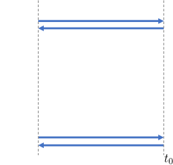
separated diagram

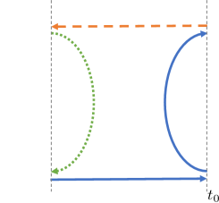
box diagram

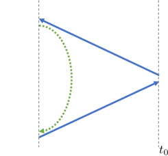
triangle diagram

Figure 1: Representative diagrams appear in correlation functions. Blue solid, orange dashed and green dotted lines are quark propagators calculated by the one-end trick, sequential propagator technique, and point-to-all propagator, respectively. The CAA is applied to the coordinates ${\bf x}$ in the box and triangle diagram.

4 Numerical result

We employ (2+1)-flavor full QCD configurations generated by the PACS-CS Collaborations [15] on a $32^{3}\times 64$ lattice with the Iwasaki gauge action[16] and a non-perturbatively improved Wilson-clover action[17]. In this setup, a lattice spacing is $a\approx 0.0907$ fm and a pion mass $m_{\pi}\approx 0.41$ GeV, where the $\rho$ meson appears as a resonance with $m_{\rho}\approx 0.89$ GeV [11]. To perform the exponential smearing at sink operators, we employ the Coulomb gauge fixing. Table 1 summarizes details of our simulations. Furthermore, to remove the dominant higher partial wave contamination of $l=3$ originated from the reduced rotational symmetry, we apply the approximated partial wave decomposition recently introduced to lattice QCD[18].

Table 1: Setups for statistics, the one-end trick and the CAA. $N_{\rm eig}$ and $N_{\rm ave}$ is the number of low eigenmodes and averaged points used in the CAA, respectively. The averaged points are chosen as ${\bf x}=(x_{0}+8l,y_{0}+8m,z_{0}+8n)\ {\rm mod}\ 32$ for $l,n,m\in\{0,1,2,3\}$, with a randomly chosen reference point ${\bf x}_{0}$ for each gauge configuration sample. Color and spinor dilutions are always used for noise vectors in the one-end trick.

Source type	$N_{\rm conf}\times N_{\rm srctime}$ (Stat. error)	One-end trick		CAA
		Noise vector	Space dilution	$N_{\rm eig}$	$N_{\rm ave}$
$\pi\pi$-type	$100\times 64$ (jackknife with bin–size 5)	$Z_{4}$ noise	$s2$ (even-odd)	300	64
$\rho$-type	$200\times 64$ (jackknife with bin–size 10)	$Z_{4}$ noise	$s4$	300	64

4.1 LO and N²LO potentials

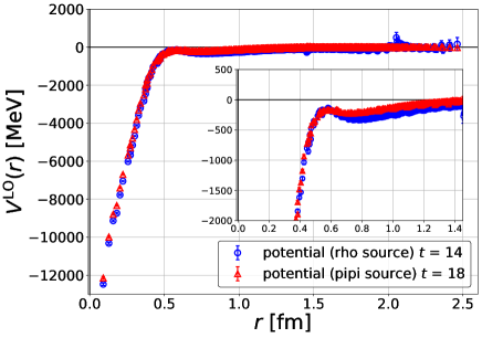
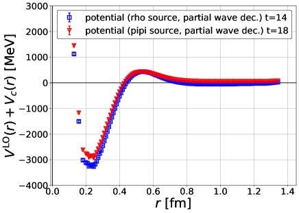
Figure 2: (Left) Effective LO potentials. Blue and red points show the results from the $\rho$-type source and the $\pi\pi$-type source, respectively. Inset shows an enlarged view of potentials. (Right) Improved potentials obtained by the partial wave decomposition[18] with the P-wave centrifugal term, $V_{c}(r)=\frac{1}{2\mu}\frac{1\cdot 2}{r^{2}}$.

Figure 2 (Left) shows the results for effective LO potentials. We observed that the potentials are attractive at all distances. We also notice that potentials obtained from different source operators are different from each other, suggesting a presence of non-negligible higher-order contributions in the derivative expansion. Fig. 2 (Right) gives potentials after the partial wave decomposition with the P-wave centrifugal term added, which become much smoother as multi-valued structures are eliminated. The potentials with the centrifugal term show characteristic features for the existence of a resonance state such as an attractive pocket at short distances and a potential barrier around $r=0.5$ fm. To evaluate the physical observables, we fit the potentials with a multi-Gaussian shape, $V(r)=a_{0}e^{-(r-a_{1})^{2}/a_{2}^{2}}+a_{3}e^{-(r-a_{4})^{2}/a_{5}^{2}}+a_{6}e^{-(r-a_{7})^{2}/a_{8}^{2}}$. The systematic uncertainty of physical observables is estimated by the uncertainty of the fits at small $r$.

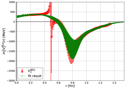
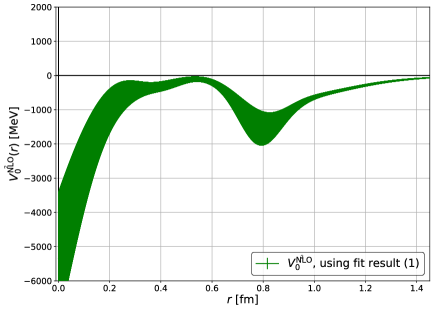
Figure 3: Effective N²LO potentials. (Left) $V_{2}^{\rm N^{2}LO}$ obtained by the decomposed data (red triangles) and fit result (green band). (Right) $V_{0}^{\rm N^{2}LO}$ obtained by fit results through the eq.(10).

Next, let us consider the N²LO potentials. The red triangle plots in Fig. 3 (Left) shows the $V_{2}^{\rm N^{2}LO}$ obtained by eq.(9). We observe a singular behavior at $r\approx 0.5$ fm, which comes from a vanishing denominator of $V_{2}^{\rm N^{2}LO}$. In the fit of $V_{2}^{\rm N^{2}LO}$, we assume that the N⁴LO or higher-order contribution in the derivative expansion can be neglected. This assumption leads us to employ a smooth fit function (same as the LO potentials) and use data points satisfying $1-2\mu V_{2}^{\rm N^{2}LO}>0$. The fit result is shown as a green band in Fig. 3 (Left). We then obtain $V_{0}^{\rm N^{2}LO}$ by combining all the fit results in eq.(10), which are shown in Fig.3 (Right). Thanks to the new strategy to handle all-to-all propagators, we succeed in extracting the effective N²LO potential of this system for the first time.

4.2 Physical observables

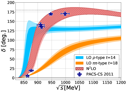
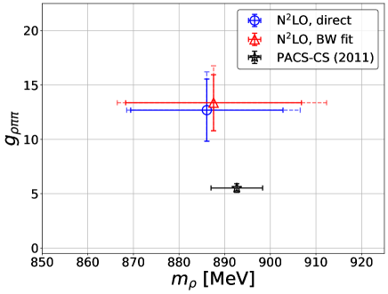
Figure 4: (Left) Scattering phase shift obtained by the LO and N²LO potentials. Lighter color bands show the systematic uncertainty estimated by the uncertainty of the fits at small $r$. (Right) A comparison of N²LO resonance parameters and previous result from PACS-CS(2011). Dotted bars give the systematic uncertainty.

Scattering phase shifts obtained by the LO and N²LO potentials are summarized in Fig.4 (Left), together with the previous result from PACS-CS Collaboration[11]. All of our results show a typical resonant behavior, rising and crossing 90 degrees. The LO results, however, largely deviate from the result of Lüscher’s method. It indicates that the LO approximation is insufficient in our setup. On the other hand, the N²LO result becomes roughly consistent with the PACS-CS result. The remaining difference between the N²LO and the PACS-CS result observed in the low-energy region can be understood as follows: Our calculations are performed only in the center-of-mass frame, where the corresponding energy levels on the current lattice volume do not cover the low-energy region near the $\pi\pi$ threshold. Therefore, the N²LO approximation could suffer from the large truncation error of the derivative expansion in such a low-energy region.

Finally, we extract parameters of the $\rho$ resonance using the N²LO potential. We employ two different procedures, fit of the Breit-Wigner parametrization and direct pole search of the S-matrix. Extracted parameters are summarized in Fig.4 (Right). The resonance mass $m_{\rho}$ is consistent with the previous study, but the coupling $g_{\rho\pi\pi}$ is twice as large. We suspect that this difference mainly comes from the discrepancy in a low-energy region as mentioned above. While a resonance mass is likely to be well reproduced as long as the resonance appears in the energy region accessible in the center-of-mass frame, the coupling may suffer from larger systematics since it is sensitive to energy dependence on a much wider range around the resonance. This observation gives us a useful lesson for the study of P-wave (or higher partial wave) resonances by the HAL QCD method with the center-of-mass frame. If the non-locality of the potential happens to be large, the truncation errors could be large at low-energies near the threshold. To control the systematics appearing in the determination of the effective coupling and decay width, one may, for example, introduce the laboratory frame calculations in the analysis or tune lattice parameters (box size etc.) to cover an energy region of a target resonance only by the center-of-mass frame spectra.

5 Summary

We study the P-wave $I=1$ $\pi\pi$ interaction at $m_{\pi}\approx 0.41$ GeV, where the $\rho$ meson appears as a resonance with $m_{\rho}\approx 0.89$ GeV. We newly introduce a combination of the one-end trick, the sequential propagator technique, and the CAA in the evaluation of correlation functions. Thanks to those techniques, we successfully determine the HAL QCD potential at the N²LO of the derivative expansion for the first time and find the pole structure corresponding to the $\rho$ resonance. The resonance mass is consistent with the previous result by Lüscher’s method, but somewhat larger coupling and decay width are obtained. We suspect that this discrepancy comes from the large systematics in the low-energy region far from the center-of-mass energy spectra, which may be reduced by, for instance, introducing the laboratory frame calculations. Although there remain some issues to be investigated, this study shows that we can study hadronic resonances requiring all-to-all calculations at the N²LO level in the HAL QCD method.

References

- [1] N. Ishii, S. Aoki and T. Hatsuda, The Nuclear Force from Lattice QCD, Phys. Rev. Lett. 99 (2007) 022001 [nucl-th/0611096].
- [2] S. Aoki, T. Hatsuda and N. Ishii, Theoretical Foundation of the Nuclear Force in QCD and its applications to Central and Tensor Forces in Quenched Lattice QCD Simulations, Prog. Theor. Phys. 123 (2010) 89 [0909.5585].
- [3] S. Aoki, Hadron interactions in lattice QCD, Prog. Part. Nucl. Phys. 66 (2011) 687 [1107.1284].
- [4] N. Ishii, S. Aoki, T. Doi, T. Hatsuda, Y. Ikeda, T. Inoue, K. Murano, H. Nemura and K. Sasaki, Hadron–hadron interactions from imaginary-time Nambu–Bethe–Salpeter wave function on the lattice, Phys. Lett. B 712 (2012) 437 [1203.3642].
- [5] J. Foley, K. Jimmy Juge, A. O’Cais, M. Peardon, S.M. Ryan and J.-I. Skullerud, Practical all-to-all propagators for lattice QCD, Comput. Phys. Commun. 172 (2005) 145 [hep-lat/0505023].
- [6] Y. Akahoshi, S. Aoki, T. Aoyama, T. Doi, T. Miyamoto and K. Sasaki, The HAL QCD potential in system with the meson bound state, PTEP 2020 (2020) 073B07 [2004.01356].
- [7] Y. Akahoshi, S. Aoki, T. Aoyama, T. Doi, T. Miyamoto and K. Sasaki, potential in the HAL QCD method with all-to-all propagators, PTEP 2019 (2019) 083B02 [1904.09549].
- [8] C. McNeile and C. Michael, Decay width of light quark hybrid meson from the lattice, Phys. Rev. D 73 (2006) 074506 [hep-lat/0603007].
- [9] G. Martinelli and C.T. Sachrajda, A Lattice Study of Nucleon Structure, Nucl. Phys. B 316 (1989) 355.
- [10] E. Shintani, R. Arthur, T. Blum, T. Izubuchi, C. Jung and C. Lehner, Covariant approximation averaging, Phys. Rev. D 91 (2015) 114511 [1402.0244].
- [11] S. Aoki et al., Meson Decay in 2+1 Flavor Lattice QCD, Phys. Rev. D 84 (2011) 094505 [1106.5365].
- [12] Y. Akahoshi, S. Aoki and T. Doi, Emergence of the resonance from the HAL QCD potential in lattice QCD, Phys. Rev. D 104 (2021) 054510 [2106.08175].
- [13] K. Murano, N. Ishii, S. Aoki, T. Doi, T. Hatsuda, Y. Ikeda, T. Inoue, H. Nemura and K. Sasaki, Spin–orbit force from lattice QCD, Phys. Lett. B 735 (2014) 19 [1305.2293].
- [14] T. Iritani, S. Aoki, T. Doi, S. Gongyo, T. Hatsuda, Y. Ikeda, T. Inoue, N. Ishii, H. Nemura and K. Sasaki, Systematics of the HAL QCD Potential at Low Energies in Lattice QCD, Phys. Rev. D 99 (2019) 014514 [1805.02365].
- [15] S. Aoki et al., 2+1 Flavor Lattice QCD toward the Physical Point, Phys. Rev. D 79 (2009) 034503 [0807.1661].
- [16] Y. Iwasaki, Renormalization Group Analysis of Lattice Theories and Improved Lattice Action: Two-Dimensional Nonlinear O(N) Sigma Model, Nucl. Phys. B 258 (1985) 141.
- [17] B. Sheikholeslami and R. Wohlert, Improved Continuum Limit Lattice Action for QCD with Wilson Fermions, Nucl. Phys. B 259 (1985) 572.
- [18] T. Miyamoto, Y. Akahoshi, S. Aoki, T. Aoyama, T. Doi, S. Gongyo, and K. Sasaki, Partial wave decomposition on the lattice and its applications to the HAL QCD method, Phys. Rev. D 101 (2020) 074514 [1906.01987].
- [19] T. Amagasa et al., Sharing lattice QCD data over a widely distributed file system, J. Phys. Conf. Ser. 664 (2015) 042058.
- [20] S. Ueda et al., Development of an object oriented lattice QCD code ’Bridge++’, J. Phys. Conf. Ser. 523 (2014) 012046.
- [21] I. Kanamori and H. Matsufuru, Practical Implementation of Lattice QCD Simulation on SIMD Machines with Intel AVX-512, Lect. Notes Comput. Sci. 10962 (2018) 456 [1811.00893].