Three-dimensional Gross-Neveu model with two flavors of staggered fermions

Abstract

We introduce a strongly interacting lattice field theory model containing two flavors of massless staggered fermions with two kind of interactions: (1) a lattice current-current interaction, and (2) an on-site four-fermion interaction. At weak couplings, we expect a massless fermion phase since our interactions become irrelevant at long distances. At strong couplings, based on previous studies, we argue that our lattice model contains two different massive fermion phases with different mechanisms of fermion mass generation. In one phase, fermions become massive through Spontaneous Symmetry Breaking (SSB) via the formation of a fermion bilinear condensate. In the other phase, fermion mass arises through a more exotic mechanism without the formation of any fermion bilinear condensate. Our lattice model is free of sign problems and can be studied using the fermion bag algorithm. The longer term goal here is to study both these mass generation phenomena in a single model and understand how different phases come together.

1 Introduction

The traditional approach for massless fermions to acquire mass is through the formation of fermion bilinear condensates. In the standard model of particle physics, this occurs through the mechanism of spontaneous symmetry breaking (SSB), which gives masses to quarks and leptons [1]. In the electro-weak sector of the Standard Model, the Higgs field plays a central role in generating masses for fermions through Yukawa couplings [2]. Due to SSB of the electro-weak symmetry, the Higgs field gets an expectation value, which gives rise to fermion bilinear mass terms in the low energy effective theory. In the strong interaction sector, spontaneous breakdown of chiral symmetries is responsible to create a fermion bilinear quark condensate. On the other hand, studies of lattice Yukawa models have found exotic phases at strong couplings [3, 4], where fermions seem to acquire mass without breaking of any symmetries of the theory. Such phases have been called the paramagnetic strong phase (PMS-phase) to contrast it with the phase at weak couplings where fermions remain massless due to lack of any symmetry breaking, which is referred to as the paramagnetic weak phase (PMW-phase). In the PMS phase, all fermion bilinear condensates vanish, but fermions are still massive [5, 6]. The traditional spontaneously broken phase is called the ferromagnetic phase (FM-phase).

In this work, we introduce a new lattice field theory model with four-fermion interactions to explore all these three phases under one framework. An important feature of our model is that it is free from sign problems and can be studied using the fermion bag algorithms without introducing a bare mass for the fermions [7]. We focus on $2+1$ dimensions, since the four-fermion interactions are known to produce many interesting quantum critical points. For example, in the so-called lattice Thirring model with a current-current interaction $U$, an interesting second order phase transition between the PMW and FM phases was observed even with a single flavor of staggered fermions [8, 9]. With two flavors of staggered fermions but with a single site four-fermion interaction $U^{\prime}$, an exotic second order transition between the PMW and PMS phases was observed [10, 9]. Our model brings together both of these transitions into a single phase diagram by introducing a model with both interactions $U$ and $U^{\prime}$, thus giving us a way to study how the two mechanisms for fermion mass generation can come together and if there are interesting new phase transitions between them.

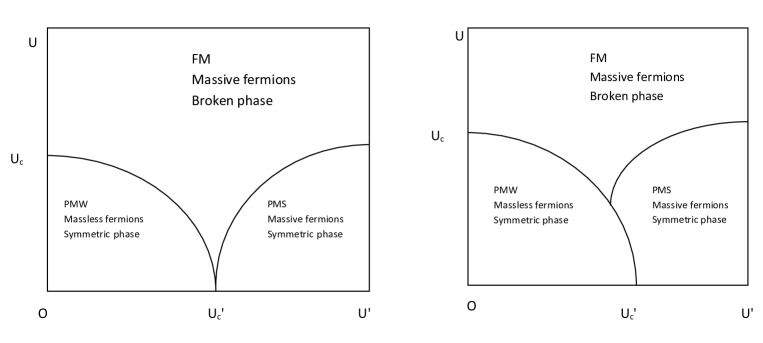
Figure 1: Two possible phase diagrams of our model, containing two types of interactions $U$ and $U^{\prime}$.

The possible phase diagrams in our model are shown in Fig. 1. The left phase diagram implies that $U=0$ is a special axis where, due to enhanced symmetries, a direct second order phase transition between PMW and PMS phase was possible. Since this generically not possible, introduction of $U$ introduces an intermediate phase. On the other hand, the right phase diagram implies that the direct phase transition between the PMW and PMS phases is more robust and is not a consequence of the special symmetries of the $U=0$ axis. Other interesting questions are related to the nature of the phase transitions between the PMW and FM phases and the PMS and FM phases. If they are second order, we can compute the critical exponents of these transitions. The nature of the multi-critical point where all the three phases meet is another possible subject for investigation.

2 Model

We study a $2+1$ dimensional lattice model containing two flavors of massless staggered fermions interacting with each other via four-fermion interactions. The Euclidean action of our model is given as a sum of three terms $S=S_{0}+S^{\text{int}}_{1}+S^{\text{int}}_{2}$, where $S_{0}$ denotes the free staggered fermion action for each of the flavors $u$ and $d$ and is given by

$$S_{0} =\sum_{\langle x,y\rangle}\left(\bar{u}_{x}M_{x,y}u_{y}+\bar{d}_{x}M_{x,y}d_{y}\right),$$ (1)

$S^{\text{int}}_{1}$ is a nearest neighbor current-current interaction term within each flavor

$$S^{\text{int}}_{1} =-U\sum_{\langle x,y\rangle}\left(\bar{u}_{x}u_{x}\bar{u}_{y}u_{y}+\bar{d}_{x}d_{x}\bar{d}_{y}d_{y}\right),$$ (2)

and $S^{\text{int}}_{2}$ is a single site interaction between the two flavors given by

$$S^{\text{int}}_{2} =-U^{\prime}\sum_{x}\left(\bar{u}_{x}u_{x}\bar{d}_{x}d_{x}\right).$$ (3)

The matrix $M$ is the massless staggered fermion matrix defined by

$$M_{x,y} =\sum\limits_{\hat{\mu}}\frac{\eta_{x,\hat{\mu}}}{2}(\delta_{x+\hat{\mu},y}-\delta_{x-\hat{\mu},y}),$$ (4)

where $x\equiv(x_{0},x_{1},x_{2})$ denotes a lattice site on a 3 dimensional cubic lattice and $\hat{\mu}$ represent unit vectors in the three directions. The $\eta_{x,\hat{\mu}}$ are the usual staggered phase factors defined as: $\eta_{x,\hat{0}}=1$, $\eta_{x,\hat{1}}=(-1)^{x_{0}}$ and $\eta_{x,\hat{2}}=(-1)^{x_{0}+x_{1}}$. When $U^{\prime}=0$, the action $S$ represents two decoupled single flavored lattice Thirring models that has been studied earlier [8]. The coupling $U^{\prime}$ couples the two flavors with each other. When $U=0$, the lattice model is the same as the one that was studied in Ref. [10].

Our lattice model has a rich internal symmetry structure. The free fermion action $S_{0}$ is symmetric under $SU(4)\times U(1)$ transformations, while $S^{\text{int}}_{1}$ is invariant under $SU(2)\times U(1)\times SU(2)\times U(1)$ and $S^{\text{int}}_{2}$ is symmetric under $SU(4)$ transformation. Hence, the action $S$ of our model is invariant under $SU(2)\times SU(2)\times U(1)$ transformations. The observables we wish to measure include local four-fermion condensates given by

$$N_{u}=\frac{2}{V}\sum_{\langle x,y\rangle}\Big{\langle}\bar{u}_{x}u_{x}\bar{u}_{y}u_{y}\Big{\rangle},\quad N_{d}=\frac{2}{V}\sum_{\langle x,y\rangle}\left\langle\bar{d}_{x}d_{x}\bar{d}_{y}d_{y}\right\rangle,\quad N_{i}=\frac{1}{V}\sum_{x}\left\langle\bar{u}_{x}u_{x}\bar{d}_{x}d_{x}\right\rangle,$$ (5)

where the sum $\langle x,y\rangle$ is over nearest neighbor bonds. Similarly, fermion bilinear susceptibilities given by

$$\chi_{uu}=\frac{1}{V}\sum_{x,y}\Big{\langle}\bar{u}_{x}u_{x}\bar{u}_{y}u_{y}\Big{\rangle},\quad\chi_{dd}=\frac{1}{V}\sum_{x,y}\Big{\langle}\bar{d}_{x}d_{x}\bar{d}_{y}d_{y}\Big{\rangle},\quad\chi_{ud}=\frac{1}{V}\sum_{x,y}\Big{\langle}\bar{u}_{x}u_{x}\bar{d}_{y}d_{y}\Big{\rangle}.$$ (6)

The symmetries of our model imply that $N_{u}=N_{d}$ and $\chi_{uu}=\chi_{dd}$. In the above expressions the expectation values are defined as

$$\left\langle\mathscr{O}\right\rangle =\frac{1}{Z}\int[\mathcal{D}\bar{u}\mathcal{D}u\mathcal{D}\bar{d}\mathcal{D}d]\hskip 2.84544pt\mathscr{O}\hskip 2.84544pte^{-S[\bar{u},u,\bar{d},d]}$$ (7)

with $Z$ being the partition function. The susceptibilities $\chi_{uu}$ and $\chi_{ud}$ diverge as $V$ in the FM-phase with non-zero fermion bilinear condensate but saturate in both the PMW phase and the PMS phase.

3 Fermion Bag Approach

The traditional approach to solve four-fermion models is by introducing an auxiliary field, where we can use the Hubbard-Stratonovich transformation to convert the four-fermion coupling into a fermion bilinear by introducing an auxiliary bosonic field [11]. Methods of gradient flow, generalizing the Lefschetz thimble method to the lattice Thirring model at finite density, have also been recently explored [12, 13]. In this work, we use an alternate approach called the Fermion Bag approach [7]. The basic idea of this alternate method is to regroup fermion worldlines inside regions denoted as fermion bags. The partition function can then be expressed as a sum over configurations of fermion bags. However, since there are several ways to regroup fermion worldlines, the approach is not unique and depending on the physics the regrouping must be done thoughtfully. When this is possible, this approach can be more efficient than the auxiliary field approach.

For our model, several possible ways to identify fermion bags. The first step involves expanding the partition function

$$Z=\int[\mathcal{D}\bar{u}\mathcal{D}u\mathcal{D}\bar{d}\mathcal{D}d]\ e^{-\sum\limits_{x,y}(\bar{u}_{x}M_{x,y}u_{y}+\bar{d}_{x}M_{x,y}d_{y})+U\sum\limits_{x,y}(\bar{u}_{x}u_{x}\bar{u}_{y}u_{y}+\bar{d}_{x}d_{x}\bar{d}_{y}d_{y})+U^{\prime}\sum\limits_{x}\bar{u}_{x}u_{x}\bar{d}_{x}d_{x}}$$ (8)

as a sum over powers of interactions, as is done in bare perturbation theory. This is done by expanding

$$e^{U\bar{u}_{x}u_{x}\bar{u}_{y}u_{y}}=(1+U\bar{u}_{x}u_{x}\bar{u}_{y}u_{y})=\sum\limits_{b_{x,y}=0,1}(U\bar{u}_{x}u_{x}\bar{u}_{y}u_{y})^{b_{x,y}}$$ (9)

$$e^{U^{\prime}\bar{u}_{x}u_{x}\bar{d}_{x}d_{x}}=(1+U^{\prime}\bar{u}_{x}u_{x}\bar{d}_{x}d_{x})=\sum\limits_{i_{x}=0,1}(U^{\prime}\bar{u}_{x}u_{x}\bar{d}_{x}d_{x})^{i_{x}}.$$ (10)

We can introduce a new set of variables representing the interactions, which in our case would be dimers or bonds $b_{x,y}$ for nearest neighbor interactions and instantons $i_{x}$ for single site interactions. Thus, every configuration $[b,i]$ divides all lattice sites into either dimers $[b]$ and $[i]$. Sites that do not belong to a dimer or an instanton will be referred to as free sites. The latter does not have any instantons or bonds. Figure 2 illustrates a configuration on a $2^{3}$ lattice.

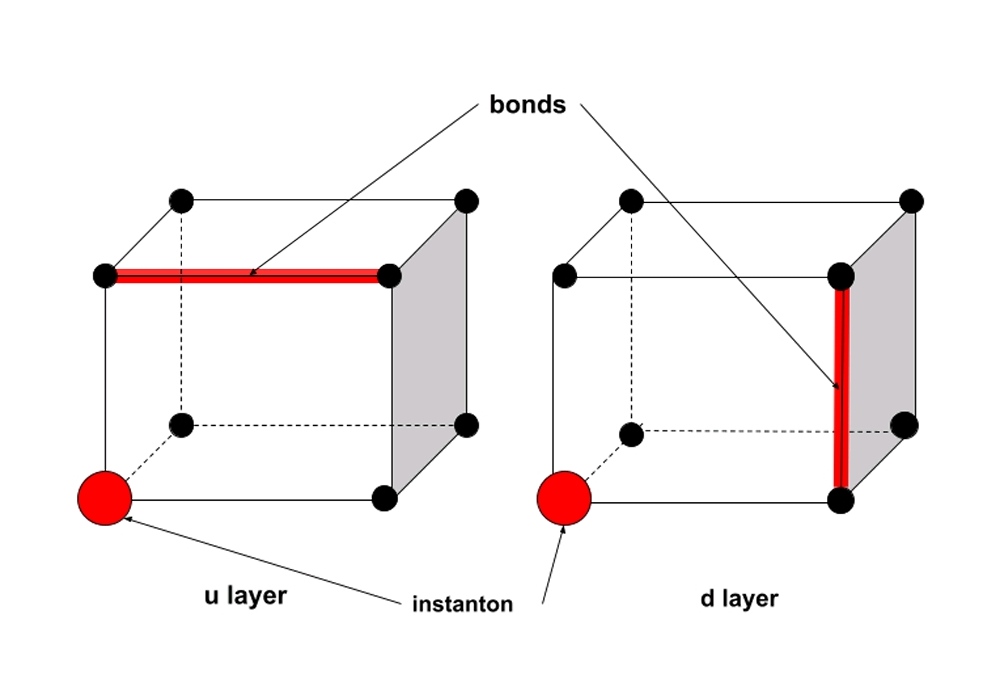
Figure 2: An illustration of a possible configuration $[b,i]$ on a $2^{3}$ lattice. The red circles denote the instanton sites and red links denote dimers. Dimers on $u$ and $d$ layers can occur on different sites, while instanton positions on both the layers are same and can be visualized as bonds connecting the two layers. The black circles denote free sites and do not contain any instantons or dimers.

One way to identify fermion bags in our model would be to group Grassmann variables that appear at every dimer or instanton and integrate them out. This gives us factors of $U$ or $U^{\prime}$ for every bond and instanton. The remaining free sites then form their own group of sites and are integrated out separately. The partition function can then be written as a sum over all configurations of $[b,i]$ as [14],

$$Z =\sum_{[b,i]}{U^{\prime}}^{N_{i}}U^{N_{u}+N_{d}}{\rm det}(W_{u})~{}~{}{\rm det}(W_{d})$$ (11)

where $N_{i}$ represents the number of instantons, while $N_{u}$ and $N_{d}$ represent the number of $u$-dimers and $d$-dimers in the configuration. The matrices $W_{u}$ and $W_{d}$ are free staggered fermion matrix restricted to the free sites. We call this approach strong coupling fermion bag since in this approach the sizes of the matrices $W_{u}$ and $W_{d}$ will be small.

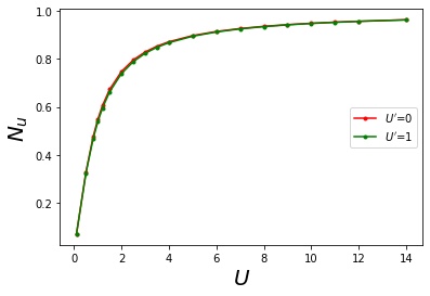
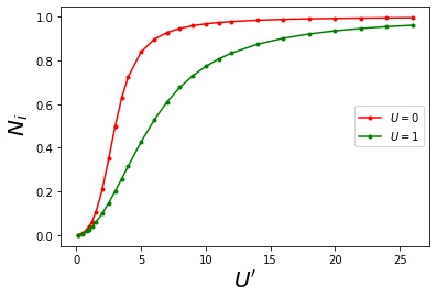
Figure 3: The variation of the average bond density ($N_{u}$) and the average instanton density ($N_{i}$) with couplings $U$ and $U^{\prime}$ for a lattice of linear dimension 2.

An alternate way of constructing the fermion bag is to consider each configuration $[b,i]$ as a term in the perturbative expansion and write the partition function as

$$Z=\sum_{[b,i]}U^{{}^{\prime}N_{i}}U^{N_{u}+N_{d}} \Bigg{\{}\int[\mathcal{D}\bar{u}\mathcal{D}u]e^{-\sum\limits_{x,y}(\bar{u}_{x}M_{x,y}u_{y})}\bar{u}_{z_{1}}u_{z_{1}}...\bar{u}_{z_{k}}u_{z_{k}}\Bigg{\}}$$

$$\times\Bigg{\{}\int[\mathcal{D}\bar{d}\mathcal{D}d]e^{-\sum\limits_{x,y}(\bar{d}_{x}M_{x,y}d_{y})}\bar{d}_{w_{1}}d_{w_{1}}...\bar{d}_{w_{\ell}}d_{w_{\ell}}\Bigg{\}}.$$ (12)

In this expression $k=2N_{u}+N_{i}$ and $\ell=2N_{d}+N_{i}$. The terms in the brackets in Eq. (12) can be computed using Wick’s theorem and summed over all contractions. This yields a simple result

$$Z =[\mathrm{det}(M)]^{2}\ \sum_{[b,i]}{U^{\prime}}^{N_{i}}U^{N_{u}+N_{d}}{\rm det}(G_{u})~{}~{}{\rm det}(G_{d})$$ (13)

where $G_{u}$ and $G_{d}$ are $k\times k$ and $\ell\times\ell$ propagator matrix between the sites $z_{1},...z_{k}$ and $w_{1},...,w_{\ell}$ respectively. We call this approach the weak coupling fermion bag, since the sizes of the matrices $G_{u}$ and $G_{d}$ will be small at weak couplings. For the efficiency of the fermion bag algorithm, it is often useful to switch between the two fermion bag formulations.

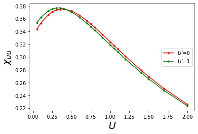
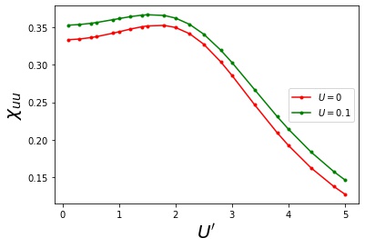
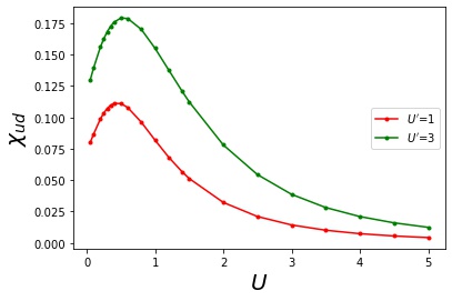
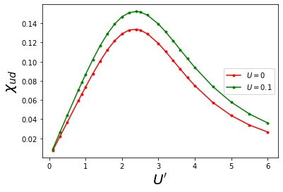
Figure 4: The behavior of $\chi_{uu}$ and $\chi_{ud}$ as a function of the couplings $U$ and $U^{\prime}$.

4 Results

We are currently developing the fermion bag Monte Carlo algorithm to explore the phase diagram of our model. In order to confirm the correctness of the algorithm, it would be useful to compare the results with exact calculations. Here we show the results from these exact calculations on a $2^{3}$ lattice size with anti-periodic boundary conditions in all three directions. The behavior of the observables $N_{u}$ and $N_{i}$ as a function of the couplings $U$ and $U^{\prime}$ are shown in Fig. 3. These four-point condensates are smooth functions, increasing from 0 for small couplings, and approaching 1 for large couplings.

To explore the phase diagram of our model further, it is more natural to study the susceptibilities $\chi_{uu}$ and $\chi_{dd}$. These are plotted as functions of the couplings $U$ and $U^{\prime}$ in Fig. 4. In the context of phase transitions, a peak in the plot of the susceptibilities as a function of the coupling for a fixed system size, can indicate a phase transition in the system. However, we must also show that the peak actually diverges in the thermodynamic limit to confirm the existence of the phase transition. As can be seen in Fig. 4, both susceptibilities show peaks. It is important to point out the fact that for very large couplings both susceptibilities as we have defined it becomes small and is related to the fact that the lattice is being filled with bonds and instantons. This however does not imply that the condensate vanishes. To measure the true condensate, we will need to study the dependence on the system size. We expect this to be dramatically different, at large U and small $U^{\prime}$ as compared to large $U^{\prime}$ and small $U$. The former will show that $\chi_{uu}$ will grow as a function of the system size while the latter will saturate. These can be inferred from previous studies.

5 Conclusions and Future work

We have introduced a three-dimensional Gross-Neveu model with two couplings $U$ and $U^{\prime}$ such that two mechanisms of fermion mass generation are possible and can compete. We have shown some exact results for $2^{3}$ lattice and already see some rudimentary features of the phase diagram. In order to understand the physics of our model in more detail, we plan to extend our results for larger lattice size using the fermion bag algorithm. We hope to explore the phase diagram of our model, and study the nature of the phase transitions. If some of these are second order, we plan to calculate the critical exponents.

References

- [1] Heather E. Logan. TASI 2013 lectures on Higgs physics within and beyond the Standard Model. 6 2014.
- [2] Antonio Pich. The Standard Model of Electroweak Interactions. In 2010 European School of High Energy Physics, pages 1–50, 1 2012.
- [3] Sinya Aoki, I-Hsiu Lee, and Robert E Shrock. Charged fermion correlation functions in a lattice scalar-fermion model with global chiral U(1) symmetry. Nuclear Physics B, 388(1):229–242, 1992.
- [4] I-Hsiu Lee, Junko Shigemitsu, and Robert E. Shrock. Study of different lattice formulations of a Yukawa model with a real scalar field. Nuclear Physics B, 334(1):265–278, 1990.
- [5] Simon Catterall. Fermion mass without symmetry breaking. JHEP, 01:121, 2016.
- [6] Ana Hasenfratz, Wei-qiang Liu, and Thomas Neuhaus. Phase Structure and Critical Points in a Scalar Fermion Model. Phys. Lett. B, 236:339–343, 1990.
- [7] Shailesh Chandrasekharan. The Fermion bag approach to lattice field theories. Phys. Rev. D, 82:025007, 2010.
- [8] Shailesh Chandrasekharan and Anyi Li. Fermion bags, duality and the three dimensional massless lattice Thirring model. Phys. Rev. Lett., 108:140404, 2012.
- [9] Shailesh Chandrasekharan and Anyi Li. Quantum critical behavior in three dimensional lattice Gross-Neveu models. Phys. Rev. D, 88:021701, 2013.
- [10] Venkitesh Ayyar and Shailesh Chandrasekharan. Massive fermions without fermion bilinear condensates. Phys. Rev. D, 91(6):065035, 2015.
- [11] F. F. Assaad, M. Bercx, F. Goth, A. Götz, J. S. Hofmann, E. Huffman, Z. Liu, F. Parisen Toldin, J. S. E. Portela, and J. Schwab. The ALF (Algorithms for Lattice Fermions) project release 2.0. Documentation for the auxiliary-field quantum Monte Carlo code. 12 2020.
- [12] Andrei Alexandru, Gokce Basar, Paulo F. Bedaque, Gregory W. Ridgway, and Neill C. Warrington. Monte Carlo calculations of the finite density Thirring model. Phys. Rev. D, 95(1):014502, 2017.
- [13] Andrei Alexandru, Paulo F. Bedaque, Henry Lamm, Scott Lawrence, and Neill C. Warrington. fermions at finite density in dimensions with sign-optimized manifolds. Phys. Rev. Lett., 121:191602, Nov 2018.
- [14] Venkitesh Ayyar, Shailesh Chandrasekharan, and Jarno Rantaharju. Benchmark results in the 2D lattice Thirring model with a chemical potential. Phys. Rev. D, 97:054501, Mar 2018.