Greybody Radiation of scalar and Dirac perturbations of NUT Black Holes

Abstract

We consider the spinorial wave equations, namely the Dirac and the Klein-Gordon equations, and greybody radiation in the NUT black hole spacetime. To this end, we first study the Dirac equation in NUT spacetime by using a null tetrad in the Newman-Penrose (NP) formalism. Next, we separate the Dirac equation into radial and angular sets. The angular set is solved in terms of associated Legendre functions. With the radial set, we obtain the decoupled radial wave equations and derive the one-dimensional Schrödinger wave equations together with effective potentials. Then, we discuss the potentials by plotting them as a function of radial distance in a physically acceptable region. We also study the Klein-Gordon equation to compute the greybody factors (GFs) for both bosons and fermions. The influence of the NUT parameter on the GFs of the NUT spacetime is investigated in detail.

I Introduction

NUT spacetimes are special case of the family of electrovac spacetimes of Petrov type-D given by the Plebański-Demiański class of solutions 1 . These axially symmetric spacetimes are characterized by the seven parameters: mass, rotation, acceleration, cosmological constant, magnetic charge, electric charge, and NUT parameter. We are interested in the solution, which is characterized by two physical parameters: the gravitational mass and the NUT parameter. From now on, we will refer to this spacetime [see metric (1)] as the NUT black hole (BH). In fact, the NUT BH is a solution to the vacuum Einstein equation that was found by Newman–Unti–Tamburino (NUT) in 1963 2 .

Since the discovery of the NUT solution, its physical meaning is a matter of debate. The interpretations of the NUT solution and thus the NUT parameter are still a controversy and it has attracted lots of attention over the years. Misner approach 3 to the interpretation of the NUT solution aims at eliminating singular regions at the expense of introducing the “periodic” time and, consequently, the $S^{3}$ topology for the hypersurfaces $r=const$. In 4 the NUT solution was interpreted as representing the exterior field of a mass located at the origin together with a semi-infinite massless source of angular momentum. Whereas in 5 the solution was interpreted as the presence of two semi-infinite counter-rotating singular regions endowed with negative masses and infinitely large angular momenta.

Regarding to the NUT parameter, in general it was interpreted as a gravitomagnetic charge bestowed upon the central mass 6 . However, the exact physical meaning has not been attained yet. In 7 it was explained that if the NUT parameter dominates the rotation parameter, then this leaves the spacetime free of curvature singularities. But if the rotation parameter dominates the NUT parameter, the solution is Kerr-like, and a ring curvature singularity arises. Conversely, exact interpretation of the NUT parameter becomes possible when a static Schwarzschild mass is immersed in a stationary, source free electromagnetic universe 8 . In this case, the NUT parameter is interpreted as a twist parameter of the electromagnetic universe. However, in the absence of this field, it reduces to the twist of the vacuum spacetime. A different interpretation of the NUT spacetime has been clarified via its thermodynamics. In 9 , it was shown that if the NUT parameter is interpreted as possessing simultaneously rotational and electromagnetic features then the thermodynamic quantities satisfy the Bekenstein-Smarr mass formula.

In article 10 , Misner called the NUT metric a ’counter-example to almost anything’: it means that it has so many peculiar properties. Following this line of thought, the aim of the present paper is to study the scalar and Dirac perturbations of the NUT BH and analyze their corresponding greybody radiation. Studies of this type have always been important in the field of quantum gravity. Furthermore, an effective way to understand and analyze characteristics of a spacetime is to study its behavior under different kinds of perturbations including spinor and gauge fields. Also, one can pave the way to study the GFs of the NUT spacetime in order to investigate the evolution of perturbations in the exterior region of the BH 11 ; 12 . The analytical expressions of the solution obtained in this paper could be useful for the study of the thermodynamical properties of the spinor fields in NUT geometry.

In the literature, the scalar/Dirac equation and greybody radiation in BH geometry have been extensively studied. For example, wave analysis of the Schwarzschild BH was performed in 13 ; 14 ; 15 ; 16 ; 17 ; 18 , for the Kerr BH in 19 ; 20 ; 21 ; 22 , for the Kerr Taub-NUT BH in 23 , for the Kerr-Newman AdS BH in 24 , and for the Reissner-Nordsrtöm de Sitter BH in 25 . Meanwhile, it is worth noting that the GFs measure the deviation of the thermal spectra from the black body or the so-called Hawking radiation 26 ; 27 . Essentially, GF is a physical quantity that relates to the quantum nature of a BH. A high value of GF shows a high probability that Hawking radiation can reach to spatial infinity (or an observer) 28 ; 29 . Today, there are different methods to compute the GF such as the matching method 30 ; 31 , rigorous bound method 32 , the WKB approximation 33 ; 34 , and analytical method for the various of spin fields 35 ; 36 ; 37 ; 38 ; 38n ; 39 ; 40 . Here, we shall employ the general method of semi-analytical bounds for the GFs. To this end, we shall examine the characteristic bosonic and fermionic quantum radiation (i.e., the GF) of NUT BH based on the current studies in the literature (see for example Harmark:2007jy ) and our recent studies 37 ; 38 ; 38n . Although the methodology followed is parallel to the procedure seen in 37 ; 38 ; 38n , due to the unique characteristics of each BH solution, the calculations have their own difficulties and therefore the results obtained will differ significantly. In those recent studies 37 ; 38 ; 38n , for example, we have revealed the effects of quintessence, negative cosmological constant, and Lorentz symmetry breaking parameters on the quantum thermal radiation of black holes. However, in this study, we aim to reveal the effect of the NUT parameter on the GF and thus present a theoretical study to the literature that will contribute to the black hole classification studies according to GF measurements that might be obtained in the (distant) future.

The paper is organized as follows: In the next section, we obtain the Dirac equation in the NUT spacetime and separate the coupled equations into the angular and radial parts. In Sect. 3, analytical solutions to the angular equations are sought. We also study the radial wave equations and examine the behaviors of the effective potential that emerge in the transformed radial equations. In Sect. 4, we study the Klein–Gordon equation in the NUT BH spacetime. Then, we derive the associated effective potential of bosons. Then, we compute the GFs of the NUT BH spacetime for both fermions and bosons in Sect. 5. We draw our conclusions in Sect. 6.

II Dirac equation in NUT BH spacetime

The NUT metric is a solution to the vacuum Einstein equation that depends on two parameters: mass $M$ and NUT parameter $l$ 1 . A detailed discussion on the NUT spacetime can be found in the famous monograph of Griffiths and Podolsky 41 and in the specific studies given in 42 ; 43 ; 44 . In spherical coordinates $(t,r,\theta,\phi)$ the NUT BH metric reads

$$ds^{2}=f(r)\left[dt-2l\cos\theta d\phi\right]^{2}-\frac{1}{f(r)}dr^{2}-\left(r^{2}+l^{2}\right)\left(d\theta^{2}+\sin^{2}\theta d\phi^{2}\right),$$ (1)

where

$$f(r)=1-\frac{2\left(Mr+l^{2}\right)}{r^{2}+l^{2}}>0.$$ (2)

The distinctive feature of the NUT metric is the presence of the NUT parameter $l$ that causes the spacetime to be asymptotically non-flat. The horizons are defined by $f(r)=0$ and hence they will occur at $r_{\pm}=M\pm\sqrt{M^{2}+l^{2}}$.

Following the NP formalism, we introduce null tetrads $(l,n,m,\overline{m})$ to satisfy orthogonality relations: $l.n=-m.\overline{m}=1.$ Thus, we write the basis vectors of null tetrad in terms of elements of the NUT geometry as follows

$$l_{\mu}=(1,-\frac{1}{f\left(r\right)},0,-2l\cos\theta),$$

$$n_{\mu}=\frac{1}{2}(f\left(r\right),1,0,-2lf(r)\cos\theta),$$

$$m_{\mu}=\sqrt{\frac{r^{2}+l^{2}}{2}}(0,0,-1,-i\sin\theta),$$

$$\overline{m}_{\mu}=\sqrt{\frac{r^{2}+l^{2}}{2}}(0,0,-1,i\sin\theta),$$ (3)

where a bar over a quantity denotes complex conjugation and the dual co-tetrad of Eq. (3) are given by

$$l^{\mu}=(\frac{1}{f\left(r\right)},1,0,0),$$

$$n^{\mu}=\frac{1}{2}(1,-f(r),0,0),$$

$$m^{\mu}=\frac{1}{\sqrt{2\left(r^{2}+l^{2}\right)}}(2il\cot\theta,0,1,\frac{i}{\sin\theta}),$$

$$\overline{m}^{\mu}=\frac{1}{\sqrt{2\left(r^{2}+l^{2}\right)}}(-2il\cot\theta,0,1,\frac{-i}{\sin\theta}).$$ (4)

Using the above null tetrad one can find the non-zero spin coefficients in terms of NUT metric:

$$\epsilon=\frac{il}{2\left(r^{2}+l^{2}\right)};\gamma=\frac{1}{4}\left(f^{\prime}(r)+\frac{ilf(r)}{r^{2}+l^{2}}\right);\alpha=-\beta=\frac{-\cot\theta}{2\sqrt{2\left(r^{2}+l^{2}\right)}}$$

$$\rho=\frac{-r+il}{r^{2}+l^{2}};\mu=\frac{f(r)}{2}\frac{-r+il}{r^{2}+l^{2}}.$$ (5)

Their corresponding directional derivatives become

$$D=l^{\mu}\partial_{\mu}=\frac{1}{f(r)}\frac{\partial}{\partial t}+\frac{\partial}{\partial r},$$

$$\Delta=n^{\mu}\partial_{\mu}=\frac{1}{2}\frac{\partial}{\partial t}-\frac{f(r)}{2}\frac{\partial}{\partial r},$$

$$\delta=m^{\mu}\partial_{\mu}=\frac{1}{\sqrt{2\left(r^{2}+l^{2}\right)}}(2il\cot\theta\frac{\partial}{\partial t}+\frac{\partial}{\partial\theta}+\frac{i}{\sin\theta}\frac{\partial}{\partial\phi}),$$

$$\bar{\delta}=\overline{m}^{\mu}\partial_{\mu}=\frac{1}{\sqrt{2\left(r^{2}+l^{2}\right)}}(-2il\cot\theta\frac{\partial}{\partial t}+\frac{\partial}{\partial\theta}-\frac{i}{\sin\theta}\frac{\partial}{\partial\phi}),$$ (6)

The Dirac equations in the curved spacetime are given by 45

$$\left(D+\epsilon-\rho\right)F_{1}+\left(\overline{\delta}+\pi-\alpha\right)F_{2}=i\mu_{\ast}G_{1},$$

$$\left(\Delta+\mu-\gamma\right)F_{2}+\left(\delta+\beta-\tau\right)F_{1}=i\mu_{\ast}G_{2},$$

$$\left(D+\overline{\epsilon}-\overline{\rho}\right)G_{2}-\left(\delta+\overline{\pi}-\overline{\alpha}\right)G_{1}=i\mu_{\ast}F_{2},$$

$$\left(\Delta+\overline{\mu}-\overline{\gamma}\right)G_{1}-\left(\overline{\delta}+\overline{\beta}-\overline{\overline{\tau}}\right)G_{2}=i\mu_{\ast}F_{1},$$ (7)

where $\mu_{\ast}$ is the mass of the Dirac particle.

The form of the Dirac equation suggests that we define the spinor fields as follows 45 ,

$$F_{1}=F_{1}\left(r,\theta\right)e^{i\left(kt+n\phi\right)},$$

$$F_{2}=F_{2}\left(r,\theta\right)e^{i\left(kt+n\phi\right)},$$

$$G_{1}=G_{1}\left(r,\theta\right)e^{i\left(kt+n\phi\right)},$$

$$G_{2}=G_{2}\left(r,\theta\right)e^{i\left(kt+n\phi\right)}.$$ (8)

where $k$ is the frequency of the incoming wave and $n$ is the azimuthal quantum number of the wave.

Substituting the appropriate spin coefficients (5) and the spinors (8) into the Dirac equation (7) , we obtain

$$\sqrt{r^{2}+l^{2}}\left(\emph{D}-\frac{il}{2\left(r^{2}+l^{2}\right)}\right)F_{1}+\frac{1}{\sqrt{2}}\mathit{L}F_{2}=i\mu_{0}\sqrt{r^{2}+l^{2}}G_{1},$$

$$\frac{f}{2}\sqrt{r^{2}+l^{2}}\left(\mathit{D}^{{\dagger}}+\frac{f^{\prime}}{2f}-\frac{il}{2\left(r^{2}+l^{2}\right)}\right)F_{2}-\frac{1}{\sqrt{2}}\mathit{L}^{{\dagger}}F_{1}=-i\mu_{0}\sqrt{r^{2}+l^{2}}G_{2},$$

$$\sqrt{r^{2}+l^{2}}\left(\emph{D}+\frac{il}{2\left(r^{2}+l^{2}\right)}\right)G_{2}-\frac{1}{\sqrt{2}}\mathit{L}^{{\dagger}}G_{1}=i\mu_{0}\sqrt{r^{2}+l^{2}}F_{2},$$

$$\frac{f}{2}\sqrt{r^{2}+l^{2}}\left(\mathit{D}^{{\dagger}}+\frac{f^{\prime}}{2f}+\frac{il}{2\left(r^{2}+l^{2}\right)}\right)G_{1}+\frac{1}{\sqrt{2}}\mathit{L}G_{2}=-i\mu_{0}\sqrt{r^{2}+l^{2}}F_{1},$$ (9)

where, $\mu_{0}=\sqrt{2}\mu_{\ast}$ and the above operators are given by

$$\emph{D}=\frac{\partial}{\partial r}+\frac{r}{r^{2}+l^{2}}+\frac{ik}{f},$$

$$\mathit{D}^{{\dagger}}=\frac{\partial}{\partial r}+\frac{r}{r^{2}+l^{2}}-\frac{ik}{f}$$

$$\mathit{L}=\frac{\partial}{\partial\theta}+\left(\frac{1}{2}+2lk\right)\cot\theta+\frac{n}{\sin\theta},$$

$$\mathit{L}^{{\dagger}}=\frac{\partial}{\partial\theta}+\left(\frac{1}{2}-2lk\right)\cot\theta-\frac{n}{\sin\theta}.$$ (10)

Further, we define $F_{1}\left(r,\theta\right)=R_{+1/2}\left(r\right)A_{+1/2}\left(\theta\right),F_{2}\left(r,\theta\right)=R_{-1/2}\left(r\right)A_{-1/2}\left(\theta\right),G_{1}\left(r,\theta\right)=R_{-1/2}\left(r\right)A_{+1/2}\left(\theta\right)$ ,$G_{2}\left(r,\theta\right)=R_{+1/2}\left(r\right)A_{-1/2}\left(\theta\right)$ hence, the set (9) can be separated into angular and radial parts as

$$\sqrt{r^{2}+l^{2}}\emph{D}R_{+1/2}=\left(\lambda+i\mu_{0}\sqrt{r^{2}+l^{2}}\right)R_{-1/2},$$ (11)

$$\frac{f}{2}\sqrt{r^{2}+l^{2}}\mathit{D}^{{\dagger}}R_{-1/2}=\left(\lambda-i\mu_{0}\sqrt{r^{2}+l^{2}}\right)R_{+1/2},$$ (12)

$$\frac{1}{\sqrt{2}}\mathit{L}A_{-1/2}=\lambda A_{+1/2},$$ (13)

$$\frac{1}{\sqrt{2}}\mathit{L}^{{\dagger}}A_{+1/2}=-\lambda A_{-1/2},$$ (14)

where $\lambda$ is the separation constant.

III Solutions of angular and radial equations

III.1 Angular equations

Angular Eqs. (14) and (13) can be written as

$$\frac{dA_{+1/2}}{d\theta}+\left(\left(\frac{1}{2}+2lk\right)\cot\theta+\frac{n}{\sin\theta}\right)A_{+1/2}=-\lambda A_{-1/2},$$ (15)

$$\frac{dA_{-1/2}}{d\theta}+\left(\left(\frac{1}{2}-2lk\right)\cot\theta-\frac{n}{\sin\theta}\right)A_{-1/2}=\lambda A_{+1/2}.$$ (16)

We note that the structure of the angular equations admits the similar solutions for both $A_{+1/2}$ and $A_{-1/2}$. Therefore, it is sufficient to focus on one of the angular equations. To this end, we apply the following transformations

$$A_{+1/2}\left(\theta\right)=\cos\left(\frac{\theta}{2}\right)S_{1}(\theta)+\sin\left(\frac{\theta}{2}\right)S_{2}(\theta),$$ (17)

$$A_{-1/2}\left(\theta\right)=-\sin\left(\frac{\theta}{2}\right)S_{1}(\theta)+\cos\left(\frac{\theta}{2}\right)S_{2}(\theta).$$ (18)

By setting $x=\cos\theta$, one can write Eq. (15) as a decoupled second order differential equation:

$$\left(1-x^{2}\right)\frac{d^{2}S_{1}}{dx^{2}}-2x\frac{dS_{1}}{dx}+\left[\lambda\left(\lambda+1\right)-\frac{\left(n+\frac{1}{2}\right)^{2}}{1-x^{2}}\right]S_{1}=0,$$ (19)

with $\left(n+\frac{1}{2}\right)^{2}\leq\lambda^{2}$. The solution to Eq. (19) can be expressed in terms of the associated Legendre functions 46 :

$$P_{\lambda}^{n}\left(x\right)=\left(1-x^{2}\right)^{\tau/2}\frac{d^{n}}{dx^{n}}P_{\lambda}\left(x\right).$$ (20)

III.2 Radial equations

The radial equations (11-12) can be rearranged as

$$\sqrt{r^{2}+l^{2}}\left(\frac{d}{dr}+\frac{r}{r^{2}+l^{2}}+\frac{ik}{f}\right)R_{+1/2}=\left(\lambda-i\mu_{0}\sqrt{r^{2}+l^{2}}\right)R_{-1/2},$$ (21)

$$\frac{f}{2}\sqrt{r^{2}+l^{2}}\left(\frac{d}{dr}+\frac{r}{r^{2}+l^{2}}+\frac{f^{\prime}}{2f}-\frac{ik}{f}\right)R_{-1/2}=\left(\lambda+i\mu_{0}\sqrt{r^{2}+l^{2}}\right)R_{+1/2}.$$ (22)

To obtain the radial equations in the form of one-dimensional Schrödinger like wave equations, we perform the following transformations

$$P_{+1/2}=\sqrt{r^{2}+l^{2}}R_{+1/2},\qquad P_{-1/2}=\sqrt{\frac{f}{2}}\sqrt{r^{2}+l^{2}}R_{-1/2}.$$ (23)

Then, Eqs. (21) and (22) transform to

$$\left(\frac{d}{dr}+i\frac{k}{f}\right)P_{+1/2}=\sqrt{\frac{2}{f}}\left(\frac{\lambda}{\sqrt{r^{2}+l^{2}}}-i\mu_{0}\right)P_{-1/2},$$ (24)

$$\left(\frac{d}{dr}-i\frac{k}{f}\right)P_{-1/2}=\sqrt{\frac{2}{f}}\left(\frac{\lambda}{\sqrt{r^{2}+l^{2}}}+i\mu_{0}\right)P_{+1/2},$$ (25)

and defining the tortoise coordinate $r_{\ast}$ as $\frac{dr_{\ast}}{dr}=\frac{1}{f}$, Eqs. (24) and (25) become

$$\left(\frac{d}{dr_{\ast}}+ik\right)P_{+1/2}=\sqrt{2f}\left(\frac{\lambda}{\sqrt{r^{2}+l^{2}}}-i\mu_{0}\right)P_{-1/2}$$ (26)

$$\left(\frac{d}{dr_{\ast}}-ik\right)P_{-1/2}=\sqrt{2f}\left(\frac{\lambda}{\sqrt{r^{2}+l^{2}}}+i\mu_{0}\right)P_{+1/2}$$ (27)

In order to write Eqs. (26) and (27) in a more compact form, we combine the solutions as $\psi_{+}=P_{+1/2}+P_{-1/2}$ and $\psi_{-}=P_{+1/2}-P_{-1/2}$ . After making some computations, we end up with a pair of one-dimensional Schrödinger like equations:

$$\frac{d^{2}\psi_{+}}{dr_{\ast}^{2}}+\left(4k^{2}-V_{+}\right)\psi_{+}=0,$$ (28)

$$\frac{d^{2}\psi_{-}}{dr_{\ast}^{2}}+\left(4k^{2}-V_{-}\right)\psi_{-}=0,$$ (29)

with the following effective potentials:

$$V_{\pm}=\frac{2L^{3/2}\sqrt{\Delta}}{D^{2}}\left[2L^{3/2}\sqrt{\Delta}\pm 3\mu_{0}^{2}r\Delta\pm L\left(r-M\right)\mp\frac{\Delta L}{D}\left(2\mu_{0}^{2}r\left(r^{2}+l^{2}\right)-\frac{\lambda\mu_{0}\left(r-M\right)}{2k}+2rL\right)\right],$$

$$L\left(r-M\right)\mp\frac{\Delta L}{D}\left(2\mu_{0}^{2}r\left(r^{2}+l^{2}\right)-\frac{\lambda\mu_{0}\left(r-M\right)}{2k}+2rL\right)],$$ (30)

where

$$\Delta=r^{2}-2Mr-l^{2},L=\left(\lambda^{2}+\mu_{0}^{2}r^{2}\right),D=L\left(r^{2}+l^{2}\right)-\frac{\lambda\mu_{0}}{4k}.$$ (31)

We see that the potentials (30) depend on the NUT parameter $l$. To obtain the potentials for massless fermions (neutrino), we simply set $\mu_{0}=0$ in Eq. (30), which yields

$$V_{\pm}=\frac{2\lambda\sqrt{\Delta}}{\left(r^{2}+l^{2}\right)^{2}}\left[2\lambda\sqrt{\Delta}\pm\left(r-M\right)\mp\frac{2\Delta r}{r^{2}+l^{2}}\right].$$ (32)

To study the asymptotic behavior of the potentials (30), we can expand it up to order $O\left(\frac{1}{r^{3}}\right)$. Thus, the potentials behave as

$$V_{\pm}\simeq 4\mu_{0}^{2}+8M\mu_{0}^{2}\frac{1}{r}\pm\left(6l^{2}\mu_{0}^{2}-2\lambda^{2}+\frac{\lambda\mu_{0}}{2k}\right)\frac{1}{r^{2}}+O\left(\frac{1}{r^{3}}\right).$$ (33)

From Eq. (33), we see that the first term corresponds to the constant value of the potential at the asymptotic infinity. In the second term, the mass produces the usual monopole type attractive potential. The NUT parameter in the third term represents the dipole type potential.

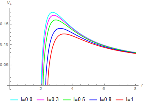
Figure 1: Graph of $V_{+}$ (30) for various values of the NUT parameter $l$. Here, $\lambda=k=1,\mu=0.12,$ and $M=0.5$.

We will now investigate the effect of the NUT parameter on the effective potentials (30) by plotting them as a function of radial distance. Figs. 1 and 2 describe the effective potentials (30) for massive particles where we obtain potential curves for some specific values of the NUT parameter. As can be seen from Figs. 1 and 2, for sufficiently small values of the NUT parameter, the potentials have sharp peaks in the physical region. When the NUT parameter $l=0$, the peak is seen to be maximum. We also observe that while the NUT parameter increases, the sharpness of the peaks decreases, and the peaks tend to disappear after a specific value of the NUT parameter. This implies that for a large values of the NUT parameter, a massive Dirac particle moving in the physical region experiences a potential barrier without peaks and its kinetic energy increases. But for a small value of the NUT parameter, it feels a sharp potential barrier.

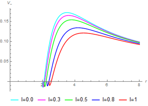
Figure 2: Graph of $V_{-}$ (30) for various values of NUT parameter $l$. Here, $\lambda=k=1,\mu=0.12,$ and $M=0.5$.

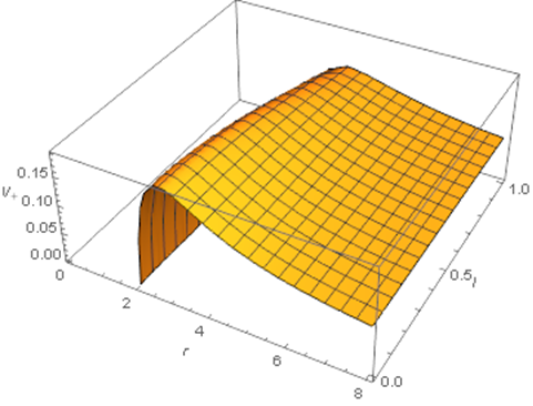
Figure 3: Three-dimensional plot of $V_{+}$ for various values of NUT parameter $l$. Here, $\lambda=k=1,\mu=0.12,$ and $M=0.5$.

Explicitly, the influence of the NUT parameter is shown in the three-dimensional plots of the potentials with respect to the NUT parameter and the radial distance. As can be seen from Fig. (3), we observe a peak for small values of the NUT parameter and as the value of the NUT parameter increases, the potentials decrease. Let us note that, for massless Dirac particle $\left(\mu_{0}=0\right)$, the potentials have similar behaviors as for the massive case.

IV Greybody Radiation from NUT BH

IV.1 Klein-Gordon equation

The Klein-Gordon equation for the massless scalar field in curved coordinates is given by isepjc

$$\square\Psi=\frac{1}{\sqrt{-g}}\partial_{\mu}\sqrt{-g}g^{\mu\nu}\partial_{\nu}\Psi=0,$$ (34)

where $g$ is the determinant of the spacetime metric (1): $\sqrt{-g}=\left(r^{2}+l^{2}\right)\sin\theta$. To separate the variables in equation (34), we assume the solutions to the wave equation in the form

$$\Psi=R\left(r\right)\Theta\left(\theta\right)\exp\left(-i\omega t\right)\exp\left(im\phi\right),$$ (35)

where $\omega$ denotes the frequency of the wave and $m$ is the azimuthal quantum number. Therefore, the Klein-Gordon equation (34) becomes

$$\left(\frac{\left(r^{2}+l^{2}\right)^{2}}{\Delta}-\frac{4l^{2}\cos^{2}\theta}{\sin^{2}\theta}\right)\omega^{2}+\frac{1}{R\left(r\right)}\frac{d}{dr}\left(\Delta\frac{dR\left(r\right)}{dr}\right)+$$

$$\frac{1}{\Theta\left(\theta\right)}\frac{1}{\sin\theta}\frac{d}{d\theta}\left(\sin\theta\frac{\partial\Theta\left(\theta\right)}{\partial\theta}\right)-\frac{m^{2}}{\sin^{2}\theta}-\frac{4l\cos\theta}{\sin^{2}\theta}\omega m=0.$$ (36)

The angular part satisfies

$$\frac{1}{\sin\theta}\frac{d}{d\theta}\left(\sin\theta\frac{\partial\Theta\left(\theta\right)}{\partial\theta}\right)-\left(\frac{4l^{2}\cos^{2}\theta+4l\omega m\cos\theta+m^{2}}{\sin^{2}\theta}\right)\Theta\left(\theta\right)=-\lambda\Theta\left(\theta\right),$$ (37)

where it has solutions in terms of the oblate spherical harmonic functions having eigenvalues $\lambda$ 46 . Therefore, the Klein–Gordon equation (36) is left with the radial part

$$\frac{d}{dr}\left(\Delta\frac{d}{dr}R\left(r\right)\right)+\left(\left(r^{2}+l^{2}\right)^{2}\omega^{2}-\Delta\lambda\right)R\left(r\right)=0.$$ (38)

By changing the variable in a new form as $R\left(r\right)=\frac{U\left(r\right)}{\sqrt{r^{2}+l^{2}}},$ the radial wave equation (38) recasts into a one-dimensional Schrödinger like equation as follows

$$\frac{d^{2}U}{dr_{\ast}^{2}}+\left(\omega^{2}-V_{eff}\right)U=0,$$ (39)

in which $r_{\ast}$ is the tortoise coordinate: $\frac{dr_{\ast}}{dr}=\frac{r^{2}+l^{2}}{\Delta},$ and $V_{eff}$ is the effective potential given by

$$V_{eff}=\frac{\Delta}{\left(r^{2}+l^{2}\right)^{3}}\left(\frac{-3r^{2}\Delta}{r^{2}+l^{2}}-\lambda\left(r^{2}+l^{2}\right)-3r^{2}-4Mr-l^{2}\right).$$ (40)

Figure 4: Plots of $V_{eff}$ (40) versus $r$ for the spin-$0$ particles for various values of NUT parameter $l$. The physical parameters are chosen as; $\lambda=k=1,\mu=0.12,$ and $M=0.5$.

It is seen from (40) that the effective potential depends on the NUT parameter $l$. Fig. 4 indicates the behavior of potential (40) under the effect of NUT parameter for massless particles. As can be seen from Fig. (4), when the NUT parameter increases, peaks of the potential goes down.

IV.2 GFs of bosons

It is known that nothing can escape a BH when approaching it. But when a quantum effect is considered, the BH can radiate. This radiation is known as the Hawking radiation. We now assume that Hawking radiation is a massless scalar field (bosons) that satisfies the Klein–Gordon equation. To evaluate the GF of the NUT metric for bosons, we use 47

$$\sigma_{l}\left(\omega\right)\geq\sec h^{2}\left(\int_{-\infty}^{+\infty}\wp dr_{\ast}\right),$$ (41)

in which $r_{\ast}$ is the tortoise coordinate and

$$\wp=\frac{1}{2h}\sqrt{\left(\frac{dh\left(r_{\ast}\right)}{dr_{\ast}}\right)^{2}+(\omega^{2}-V_{eff}-h^{2}\left(r_{\ast}\right))^{2}},$$ (42)

where $h(r\ast)$ is a positive function satisfying $h\left(-\infty\right)=h\left(-\infty\right)=\omega$: see Refs. 47 ; 48 for more details. Without loss of generality, we select $h=\omega$. Therefore,

$$\sigma_{l}\left(\omega\right)\geq\sec h^{2}\left(\int_{r_{h}}^{+\infty}\frac{V_{eff}}{2\omega}dr_{\ast}\right).$$ (43)

We use the potential derived in (40) to obtain the GFs for bosons, namely

$$\sigma^{s}_{l}\left(\omega\right)\geq\sec h^{2}\frac{1}{2\omega}\int_{r_{h}}^{+\infty}\frac{1}{\left(r^{2}+l^{2}\right)}\left(\frac{-3r^{2}\Delta}{\left(r^{2}+l^{2}\right)^{2}}+\lambda+\frac{\Delta^{\prime}{r}+\Delta}{r^{2}+l^{2}}\right)dr.$$ (44)

After integration, we obtain

$$\sigma^{s}_{l}\left(\omega\right)\geq\sec h^{2}\frac{1}{2\omega}{\left(\frac{-\lambda}{r}-\frac{M}{r^{2}}+\frac{l^{2}\left(\lambda-5\right)}{3r^{3}}+\frac{5Ml^{2}}{2r^{4}}+\frac{l^{4}\left(16-\lambda\right)}{5r^{5}}+\frac{l^{6}\left(\lambda-3\right)}{7r^{7}}\right)}.$$ (45)

The behaviors of the obtained bosonic GFs of the NUT BH are depicted in Fig. 5 in which the plots of $\sigma\left(\omega\right)$ for various values of NUT parameter. As can be seen from those graphs, the NUT has an effect on the bosonic GFs. Remarkably, $\sigma\left(\omega\right)$ clearly decreases with the increasing NUT parameter. In other words, the NUT plays a kind of booster role for the GFs of the spin-0 particles.

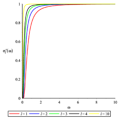
Figure 5: Plots of $\sigma^{s}_{l}\left(\omega\right)$ (45) versus $\omega$ for the zero spin particles for various values of NUT parameter $l$. The physical parameters are chosen as; $\lambda=2$ and $M=1$.

IV.3 GFs of fermions

Here, we shall derive the fermionic GF of the neutrinos emitted from the NUT BH. To this end, we consider the potentials (32). Following the procedure described above [see Eqs. (41)-(43)], we obtain,

$$\sigma_{\pm}\left(\omega\right)\geq\sec h^{2}\frac{\lambda}{\omega}\left(-\frac{2\lambda\mp 1}{r}\mp\left(\frac{M}{r^{2}}+\frac{M^{2}-l^{2}\mp 4l^{2}\lambda}{6r^{3}}\right)\pm\frac{3M^{3}-Ml^{2}}{8r^{4}}\right).$$ (46)

The fermionic GFs of the NUT BH are depicted in Figs. 6 and 7 in which the plots of $\sigma_{\pm}\left(\omega\right)$ for various values of NUT parameter are obtained. Similar to the bosonic GFs, the NUT has an intensifier effect on the GFs of the spin-$\frac{1}{2}$ particles.

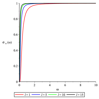
Figure 6: Plots of $\sigma_{+}\left(\omega\right)$ (45) versus $\omega$ for the Non-zero spin particles for various values of NUT parameter $l$. The physical parameters are chosen as; $\lambda=-0.5$ and $M=1$.

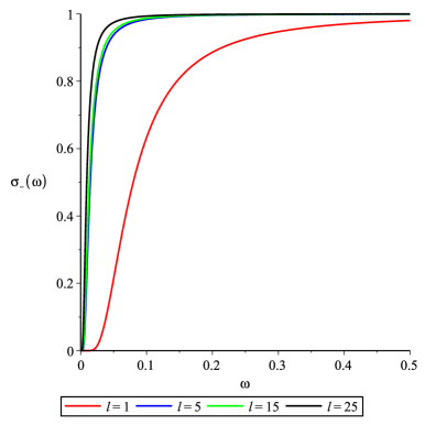
Figure 7: Plots of $\sigma_{-}\left(\omega\right)$ (46) versus $\omega$ for the Non-zero spin particles for various values of NUT parameter $l$. The physical parameters are chosen as; $\lambda=-0.5$ and $M=1$.

V Conclusion

We have studied the perturbation and greybody radiation in the NUT spacetime. The NUT metric describes the vacuum spacetime around a source that is characterized by two parameters, the mass of the central object and the NUT parameter. The perturbations studied here are for the bosons and fermions, namely the Klein-Gordon and Dirac equations are considered. For the Dirac equation, we explicitly work out the separability of the equations into radial and angular parts by using a null tetrad in the NP formalism. It is shown that solutions to the angular equations could be given in terms of the associated Legendre functions. We also discussed the radial equations and obtain a wave equation with an effective potential. The radial part involves both mass and NUT parameters. It is shown in the asymptotic expansion of the potentials (33) that the mass produces the usual $1/r$ attractive potential while the NUT parameter manifests itself in the $1/r^{2}$ asymptotically. Thus, the effect of gravity is as expected stronger than the effect of the NUT parameter in the NUT geometry. To understand the physical interpretations of the potentials (30), we make two- and three-dimensional plots of the potentials for different values of the NUT parameter. It is seen from the plots that the potential barriers are higher for small values of the NUT parameter. If the NUT parameter decreases, the peak of the potential barriers distinctly increases. Potentials become limited regardless of the value of the NUT parameter and tend to a constant value for large values of distances.

For the GFs of bosons, we have considered the massless scalar wave equation. To this end, we have reduced the radial part of the Klein-Gordon equation to the one-dimensional Schrödinger like wave equation. The behaviors of the effective potential (40) under the effect of the NUT parameter for the scalar waves are depicted. It is seen from Fig. 4 that as the NUT parameter increases then the peak of the barrier goes down. In the sequel, we have computed the GFs, one of the fundamental information that can be obtained from the BHs, for both bosons and fermions. It has been observed from Figs. 5, 6 and 7 that increment of the NUT value significantly increases the GF radiation of both bosons and fermions.

In the cosmology, the NUT parameter measures the amount of anisotropy that a metric has at large times [50]. Therefore, the GF analyses of the rotating NUT BHs, like Kerr-NUT-de Sitter BH [50], in the AdS background shall be a significant future extension of the present work. This may also be important to understand the AdS/CFT conjecture with the NUT similar to the quasinormal modes [51] analysis of planar Taub-NUT BHs [52]. This will be investigated in a near future work.

References

• (1) J. Plebański and M. Demiański, Ann. Phys. (N.Y.) 98, 98 (1976).
• (2) Newman E T, Tamburino L and Unti T W J, J. Math. Phys. 4 915-23, (1963).
• (3) C. W. Misner, Relativity Theory and Astrophysics ed J Ehlers (Amer. Math. Soc., Providence, Rhode Island) 1, 160 (1967).
• (4) W.B. Bonnor, Proc. Camb. Philos. Soc. 66, 145 (1969).
• (5) V.S. Manko, E. Ruiz, Class. Quantum Gravity 22, 3555 (2005).
• (6) D. Lynden-Bell, M. Nouri-Zonoz, Rev. Mod. Phys. 70, 427 (1998).
• (7) Griffiths. J.B. and Padolsky.J, Class. Quant. Grav., 24, 1687. (2007).
• (8) A. Al-Badawi, M. Halilsoy, Gen. Relativ. Gravit. 38, 1729 (2006).
• (9) S.-Q. Wu, D. Wu, Phys. Rev. D 100, 101501(R) (2019).
• (10) c. Misner, Relativity Theory and Astrophysics. I. ed J Ehlers (Providence, RI: American Mathematical Society), 160 (1967).
• (11) K. D. Kokkotas and B. G. Schmidt, Living Rev. Rel. 2, 2 (1999).[gr-qc/9909058].
• (12) H. P. Nollert, Class. Quant. Grav. 16, R159 (1999).
• (13) B. Mukhopadhyay, S.K. Chakrabarti, Class. Quantum Grav. 16, 3165 (1999).
• (14) J. Jing, Phys. Rev. D 70 065004 (2004); Phys. Rev. D 71 124006 (2005).
• (15) A. Al-Badawi, M.Q. Owaidat, Gen Relativ Gravit 49,110 (2017).
• (16) I.I. Cotaescu, Mod. Phys. Lett. A 22, 2493 (2007).
• (17) W. G. Unruh, Phys. Rev. D 14, 3251 (1976).
• (18) A. Zecca, Nuovo Cimento 30, 13091315 (1998).
• (19) H. Schmid, Math. Nachr. 274275, 117129 (2004).
• (20) D. Page, Phys. Rev. D 14, 1509 (1976).
• (21) E. G. Kalnins and W. Miller, J. Math. Phys. 33, 286 (1992).
• (22) F. Belgiorno, S.L. Cacciatori, J. Phys. A 42, 135207 (2009)
• (23) H. Cebeci, N. Ozdemir, Class. Quantum Grav. 30, 175005 (2013).
• (24) F. Belgiorno, S.L. Cacciatori, J. Math. Phys. 51, 033517 (2010).
• (25) Yan Lyu and Song Cui, Phys. Scr. 79, 025001 (2009).
• (26) D.N. Page, Phys. Rev. D 13, 198 (1976).
• (27) D.N. Page, Phys. Rev. D 14, 3260 (1976).
• (28) R. Jorge, E.S. de Oliveira, J.V. Rocha, Class. Quantum Gravity 32, 065008 (2015).
• (29) J. Abedi, H. Arfaei, Class. Quantum Gravity 31, 195005 (2014).
• (30) S. Fernando, Gen. Relativ. Gravit. 37, 461 (2005).
• (31) W. Kim, J.J. Oh, JKPS 52, 986 (2008).
• (32) T. Harmark, J. Natario, R. Schiappa, Adv. Theor. Math. Phys. 14, 727 (2010).
• (33) K. Jusufi, M. Amir, M. Sabir Ali, S.D. Maharaj, Phys. Rev. D 102, 064020 (2020)
• (34) M.K. Parikh, F. Wilczek, Phys. Rev. Lett. 85, 5049 (2000).
• (35) P. Boonserm, T. Ngampitipan, P.Wongjun, Eur. Phys. J. C 79, 330 (2019).
• (36) I. Sakalli, Phys. Rev. D 94, 084040 (2016). arXiv:1606.00896 [grqc].
• (37) A. Al-Badawi, I. Sakalli, S. Kanzi, Ann. Phys. 412, 168026 (2020).
• (38) A. Al-Badawi, S. Kanzi, I. Sakalli, Eur. Phys. J. Plus 135, 219 (2020).
• (39) H. Gursel, I. Sakalli, Eur. Phys. J. C 80, 234 (2020).
• (40) S. Kanzi, S.H.Mazharimousavi, I. Sakalli, Ann. Phys. 422, 168301 (2020).
• (41) S. Kanzi, İ. Sakallı, Eur. Phys. J. C 81, 501 (2021).
• (42) T. Harmark, J. Natario, R. Schiappa, Adv. Theor. Math. Phys. 14, no.3, 727-794 (2010).
• (43) J. B. Griffiths, J. Podolsky, Exact Space-Times in Einstein’s General Relativity (Cambridge: Cambridge University Press), (2009).
• (44) Jefremov, P.I., Perlick, V.: Circular motion in NUT space-time, Class. Quantum Gravity 33, 179501 (2016).
• (45) M. Nouri-Zonoz, D. Lynden-Bell, Mon. Not. Roy. Astron. Soc. 292, 714 (1998).
• (46) M. Halla, V. Perlick, Gen. Relativ. Gravit. 52, 112 (2020).
• (47) S. Chandrasekhar, The Mathematical Theory of Black Holes Clarendon, London (1983).
• (48) M. Abramowitz, I. A. Stegun (ed.), Handbook of Mathematical Functions (Dover, New York, 1970) and [S. Detweiler, Phys. Rev. D 22, 2323 (1980)].
• (49) I. Sakalli, Eur. Phys. J. C 75, no.4, 144 (2015).
• (50) Y.G. Miao, Z.M. Xu, Phys. Lett. B 772, 542 (2017).
• (51) M. Visser, Phys. Rev. A 59, 427438 (1999). arXiv: quant-ph/9901030.
• (52) A. Anabalón, S. F. Bramberger and J. L. Lehners, JHEP 09, 096 (2019).
• (53) I. Sakalli, Mod. Phys. Lett. A 28, 1350109 (2013).
• (54) P. A. Cano and D. Pereñiguez, [arXiv:2101.10652 [hep-th]].