Coupling the motional quantum states of spatially
distant ions using a conducting wire

Abstract

Interfacing ion qubits in separate traps is among the challenges towards scaling up ion quantum computing. This theoretical study focuses on using a conducting wire to couple the motional quantum states of ions in separate planar traps. This approach of interfacing ion traps provides an alternative to coupling distant qubits with lasers. We include the effects of $1/f^{\tilde{\alpha}}$ (Anomalous) surface heating noise, using aggregate and recent experimental findings as the basis for an analytical model of the motional state decoherence time $t_{\mathrm{deco.}}$. Our optimized design for the coupling system can be used to exchange quantum information with a time $t_{\mathrm{ex.}}$ less than one tenth of the information decay time $t_{\mathrm{deco.}}$. To maximize the coupling strength $\gamma$, we find a rule of thumb to relate the distance $d_{\mathrm{eq.}}$ between a trapped ion and a nearby pickup disk, to the optimal radius $r_{\mathrm{opt.}}$ of the disk, $d_{\mathrm{eq.}}/\sqrt{2}\leq r_{\mathrm{opt.}}\leq d_{\mathrm{eq.}}$. We derive a coefficient $\zeta$ which relates the capacitances of each part of the coupling system and corrects an oversight common to several previous works. Where possible, we calculate the classical signal strength and classical noise strength, and use the criterion (classical) signal-to-noise-ratio $\geq 10$ to further constrain design parameters. Ranges for all parameters are discussed, and the ratio $t_{\mathrm{deco.}}/t_{\mathrm{ex.}}$ and the signal-to-noise ratio for thermal noise are plotted to assess specific parameter ranges for which transfer of quantum information is possible. Although $1/f^{\tilde{\alpha}}$ surface noise significantly constrains parameter ranges, we find no barriers to exchanging quantum information between ion qubits in separate surface traps using a conducting wire. Moreover, this should be possible using existing technologies and materials, and singly-charged ions.

Qubits are the basic unit of information of today’s quantum computers. They can be created using a variety of physical systems, much as normal (non-quantum) information bits can be made from small magnets as was once done in floppy disks, or burn marks on CDs, or transistor logic. Among front-running qubit candidates, trapped ions are of particular interest due to their long lifetimes, with demonstrated $T_{2}$ coherence times over $\sim 50$ seconds at the time of writing (without dynamical decoupling)Gaebler et al. (2016); Harty et al. (2014). They are suitable for performing quantum gate operations in their own right, and have the potential to complement other technologies such as superconducting qubits, which have faster gate times on the order of tens of nanoseconds Noguchi et al. (2020); Barends et al. (2014); Bruzewicz et al. (2019). One of the barriers to scaling trapped ion quantum computing is the number of qubits that can be made to interact coherently in a single trapping device Brown et al. (2016); Bruzewicz et al. (2019); Landsman et al. (2019a). This has motivated research into ways to exchange quantum information between ion qubits in separate traps, for example using ion shuttling Kaufmann et al. (2014); Kaushal et al. (2020); Wan et al. (2020); Pino et al. (2020), or photonic interconnects Landsman et al. (2019b); Stute et al. (2012); Monroe et al. (2014). Another strategy is to couple the motion of a trapped ion to a nearby conducting wire which leads to another ion Heinzen and Wineland (1990); Daniilidis et al. (2009); Zurita-Sánchez and Henkel (2008); Marzoli et al. (2009); Liang and Ke-Lin (2010); Kotler et al. (2017); Rica et al. (2018). The three techniques above have been met with varying degrees of success, and in particular, quantum information exchange between two ions via a conducting wire has never been achieved. For any approach to work, we introduce two general criteria that must be simultaneously satisfied.

1. The coherence time of the quantum state should exceed the time it takes to transfer the quantum state: $t_{\mathrm{deco.}}/t_{\mathrm{ex.}}\gg 1$

2. The amplitude of the signal carrier (Coulomb interaction, voltage, current, photons, etc.) must exceed the amplitude of the noise which arises throughout the transfer process: Signal / Noise $\gg 1$

These statements elaborate on the DiVincenzo criteria for quantum communication DiVincenzo (2000). Here, we consider the scheme of a conducting wire which guides the exchange of quantum information between two ions. The two criteria above serve as guiding principles which motivate us to calculate four quantities: i) the time $t_{\mathrm{ex.}}$ required to exchange quantum information via a conducting wire, ii) the coherence time $t_{\mathrm{deco.}}$ of the motional mode of an ion qubit, iii) the classical voltage signal, $V_{\mathrm{sig.}}$, iv) the classical Johnson-Nyquist (thermal) noise voltage $V_{\mathrm{J.N.}}$.

A limited number of works have studied systems similar to the design developed herein Zurita-Sánchez and Henkel (2008); Liang and Ke-Lin (2010); Daniilidis et al. (2009) and calculated exchange times $t_{\mathrm{ex.}}$ for those systems. To our knowledge, this is the first work that includes $1/f^{\tilde{\alpha}}$ (Anomalous) surface heating noise in an analytical model for the coherence time $t_{\mathrm{deco.}}$ of the motional state of trapped ions. Estimating $t_{\mathrm{deco.}}$ analytically has only recently become possible as a result of aggregate Schmidt-Kaler et al. (2003); Deslauriers et al. (2006); Epstein et al. (2007); Lucas et al. (2007); Labaziewicz et al. (2008); Hite et al. (2012); Chiaverini and Sage (2014); Daniilidis et al. (2014) and recent Bruzewicz et al. (2015); Talukdar et al. (2016); Sedlacek et al. (2018a, b); An et al. (2019) experimental measurements of $1/f^{\tilde{\alpha}}$ heating, which is often the dominant source of motional state decoherence. We use experimental findings as the basis for a comprehensive, empirically motivated analytical model of $1/f^{\tilde{\alpha}}$ heating. This model is used to estimate the coherence time $t_{\mathrm{deco.}}$ of the motional mode of an ion qubit, and arrive at an analytical model for the ratio $t_{\mathrm{deco.}}/t_{\mathrm{ex.}}$. Careful design of the coupling system can be used to maximize $t_{\mathrm{deco.}}/t_{\mathrm{ex.}}$ by enhancing the coupling strength $\gamma$ between two ions, which minimizes the information exchange time $t_{\mathrm{ex.}}$. Strategic choices of experimental parameters can also be used to maximize the ratio $t_{\mathrm{deco.}}/t_{\mathrm{ex.}}$ by maximizing the coherence time $t_{\mathrm{deco.}}$. Additionally, we find an analytical expression for the ratio $V_{\mathrm{sig.}}/V_{\mathrm{J.N.}}$ and use it to further constrain design parameters. This analysis and relevant surrounding considerations pave the way towards simultaneously meeting the two general criteria above. By extension, the analysis and methodology developed herein are expected to be useful for a diverse range of experiments aimed at transferring quantum information using the motional states of trapped ions, and interfacing trapped ions with nearby conductors.

The study is organized into six sections. In section I) we calculate the charge $Q_{\mathrm{transf.}}$ induced on a grounded conductor. Section II) uses the result from section I) to find the coupling strength $\gamma$ between two charges in separate traps. We compare the coupling strength calculated here with the coupling strengths calculated in other studies. In section III) we estimate classical signals induced in the coupling system, and discuss various types of noise including $1/f^{\tilde{\alpha}}$ surface heating. Section IV) uses experiments in the literature to introduce an analytical model for $1/f^{\tilde{\alpha}}$ noise. The model for $1/f^{\tilde{\alpha}}$ noise is used to estimate the decoherence time $t_{\mathrm{deco.}}$ of motional quantum information in the ion, and to find parameter ranges which simultaneously satisfy the decoherence constraint $t_{\mathrm{deco.}}/t_{\mathrm{ex.}}\geq 10$ and the signal-to-noise-ratio constraint, $V_{\mathrm{sig.}}/V_{\mathrm{J.N.}}\geq 10$, where $V_{\mathrm{J.N.}}$ is the Johnson-Nyquist (thermal) noise voltage. In section V) we discuss ways to implement a practical system, and consider decoherence of quantum information in the coupling wire. Section VI) summarizes our conclusions and outlook.

I Induced charge and current in a grounded system

I.1 Establishing the relevant quantities

We begin with a brief refresher of electrostatics in conductors. Everywhere within a conductor, the electric field is zero at equilibrium. This means the potential $V$ within a conductor, which is related to the electric field by $\vec{E}=\vec{\nabla}V$,  is either a constant, or zero. However, the charge-density on the surface of a conductor can (and must) vary arbitrarily along the surface. Even if a conductor is grounded, in general the local charge-density on the surface is not zero or homogeneous, as charges near the surface must rearrange to ensure that any $\vec{E}$-field outside the conductor is canceled off to zero within the conductor Griffiths (1962a).

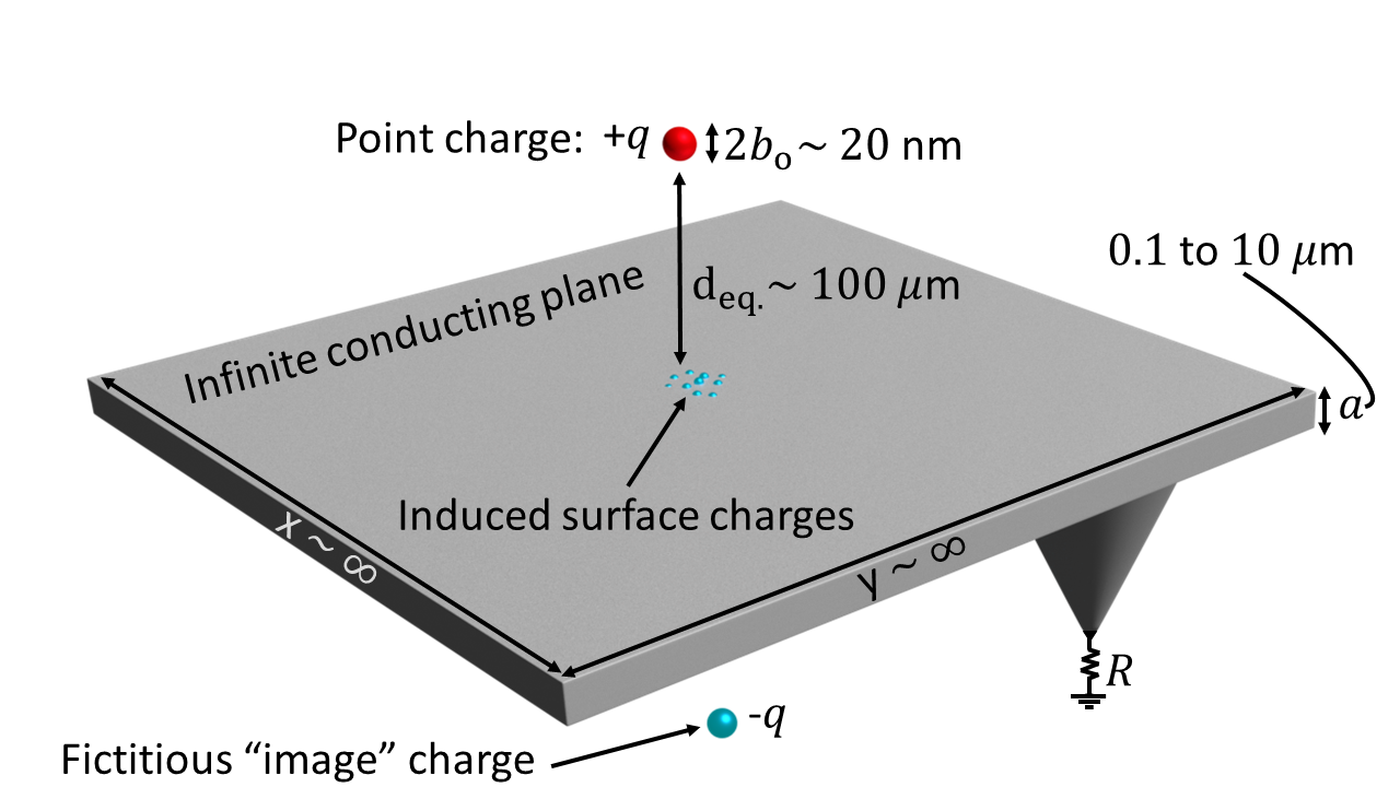
Figure 1: Charged particle floating above a plane. Schematic diagram of a positive charge (red) suspended above an infinite grounded conducting plane. The positive charge causes negative charges (small blue dots) to accumulate on the surface below it. The induced charge is centered around the origin of the coordinate system, ($x=0,y=0,z=0$). It can be shown that the electric field produced above the plane by the induced charges, is identical to the electric field which would be produced by a fictitious ”image” charge located at a distance $d_{\mathrm{eq.}}$ below the surface of the plane.

We start with a simple model, and proceed to fill in details as their relevance becomes apparent. Let us consider a positive point-charge $+q$ suspended above an infinite grounded conducting plane (Figure 1). According to the ”first uniqueness theorem” of electrostatics, (see Griffiths Griffiths (1962b), section 3.2.1), for any given set of boundary conditions for the voltage, along with a known charge-density distribution, there exists only one function which describes the voltage throughout the volume. This is a slight generalization of the uniqueness of solutions to Laplace’s equation, given specified boundary conditions. The two boundary conditions $V=0$ at the surface of a grounded plane, and $V=0$ far away from the plane, guarantee that a point-charge situated a distance $d$ above the conducting surface, along the $z$ axis, must produce a potential in the space above the plane given by (Griffiths (1962b), section 3.1.5):

$$V(x,y,z)= \frac{1}{4\pi\epsilon_{\mathrm{o}}}\Bigg{(}\frac{q_{\mathrm{c}}}{\sqrt{x^{2}+y^{2}+(z-d)^{2}}}$$ (1)

$$-\frac{q_{\mathrm{c}}}{\sqrt{x^{2}+y^{2}+(z+d)^{2}}}\Bigg{)}~{}.$$

where $x$ and $y$, are coordinates in the conducting plane as shown in figure 1. The induced surface-charge density on a conductor is given by:

$$\sigma=-\epsilon_{\mathrm{o}}\frac{\partial V}{\partial\hat{n}}$$ (2)

where $\hat{n}$ is the perpendicular direction to the surface of the conductor (here, $\hat{n}=\hat{z}$). Thus, for a point charge above a conducting plane, $\sigma$ is given by:

$$\sigma=-\epsilon_{\mathrm{o}}\frac{\partial V}{\partial z}\bigg{|}_{z=0}=\frac{-qd}{2\pi(x^{2}+y^{2}+d^{2})^{3/2}}$$

or

$$\sigma=\frac{-qd}{2\pi(r^{2}+d^{2})^{3/2}}$$ (3)

in cylindrical coordinates. The induced surface-charge density is negative, which ensures that the field produced by the positively charged particle is canceled off within the conducting plane. If we were to integrate the surface-charge density $\sigma$ over the whole plane, we would find the total induced charge on the surface of the conductor is $-q$. This result is independent of the distance $d$ between the point charge and the surface, which may seem counter-intuitive. However, while the total charge induced on the surface is independent of $d$ (and always adds up to $-q$), the charge distribution is not. Specifically, the surface-charge density directly below the particle increases and decreases in magnitude depending on whether the particle is brought closer to or farther away from the surface, respectively. The induced charge goes from ”dispersed” to ”localized” as the charged particle is brought closer to the surface. The change in charge-density $\sigma$ for a small change in the vertical distance $\delta d$ between the particle and the surface is given by:

$$\frac{\partial\sigma}{\partial d}=\frac{\partial}{\partial d}\left[Ad(r^{2}+d^{2})^{-3/2}\right]=A\frac{r^{2}-2d^{2}}{(r^{2}+d^{2})^{5/2}}~{},$$ (4)

where $A\equiv\frac{-q}{2\pi}$ is introduced to simplify expression (4). It is useful to take a moment to examine this expression. Three cases are of specific interest: $r\ll d,r\gg d$, and $r=d$. The first case leads to:

$$A\frac{r^{2}-2d^{2}}{(r^{2}+d^{2})^{5/2}}\to\frac{-2A}{d^{3}}~{}.$$ (5)

The second case leads to:

$$A\frac{r^{2}-2d^{2}}{(r^{2}+d^{2})^{5/2}}\to\frac{A}{r^{3}}~{}.$$ (6)

The most important point to notice is that the signs of the two expressions, (5) and (6), are opposite. This corresponds to the fact that if you are an observer situated on the plane, directly below the suspended particle (case 1, expression (5)), and the particle is moved a bit farther away from the surface (i.e. $d$ increases), you will see the negative charge density around you decrease (become less negative); however, if instead of being positioned directly below the suspended particle, you are located at some ’far away’ place (still on the surface of the plane, case 2, expression (6)), then as the particle is moved farther away from the surface you will see an increase in the negative charge density around you. This is consistent with our earlier observation that the total surface-charge adds up to a constant, $-q$. If the particle is moved closer to the surface, the increase in negative charge-density directly below the particle must come at the expense of a decrease in negative charge-density at some not-yet-specified ’farther-away’ radius. For completeness, we can mention the rather uninteresting case $r=d$. We find: $A\left(r^{2}-2d^{2}\right)/\left((r^{2}+d^{2})^{5/2}\right)\to\left(-A\right)/\left(2d^{3}\right)$.

Given that $\frac{\partial\sigma}{\partial d}$ is positive for some values of $r$ and negative for other values of $r$, a natural question is: ”When does $\frac{\partial\sigma}{\partial d}=0$?”.

Solving:

$$A\frac{r^{2}-2d^{2}}{(r^{2}+d^{2})^{5/2}}=0$$

yields:

$$r=\sqrt{2}d~{}.$$ (7)

This is the distance of zero charge-density variation. If one tries to measure a current at a distance exactly $r=\sqrt{2}d$ from the origin, no current will be measured at all. Furthermore, if the current-measuring device extends along both sides of this invisible line, it will lose sensitivity because it will simultaneously measure opposite currents, effectively canceling off a portion of the signal.

It is useful to know where on the surface the greatest current is, when the particle oscillates, so the current can be measured at that location. In other words, one would like know at what radius $\frac{\partial\sigma}{\partial d}$ is maximized as a function of $r$. The problem to solve is: $f(r)=\frac{\partial\sigma}{\partial d}(r)=max$, or:

$$\frac{\partial f(r)}{\partial r}=\frac{\partial}{\partial r}\left[A\frac{r^{2}-2d^{2}}{(r^{2}+d^{2})^{5/2}}\right]=0~{}.$$ (8)

This yields two solutions:

$$r=0,\qquad\mathrm{and}\qquad r=\pm{2d}$$ (9)

The first solution at $r=0$ is rather intuitive. Based on simple reasoning, we might guess that there should also be a second solution somewhere at $r>\sqrt{2}d$. However, that the second maximum is at $r=2d$ is not obvious. (The third solution at $r=-2d$ is not physically meaningful). Of the two solutions, one might predict that the solution at $r=0$ is where the greatest change in surface-charge density occurs. But it is good practice to verify this. We find for the solution at $r=0$:

$$\frac{\partial\sigma}{\partial d}\bigg{|}_{r=0}=A\frac{-2}{d^{3}}~{},$$ (10)

while for the solution at $r=2d$:

$$\frac{\partial\sigma}{\partial d}\bigg{|}_{r=2d}=A\frac{2}{5^{5/2}d^{3}}~{}.$$ (11)

The two solutions differ in magnitude by a factor of $\frac{1}{5^{5/2}}$, so the change in surface-charge density at $r=2d$ is approximately $~{}0.02$ times as significant as the change in surface-charge density at $r=0$. The discussion so far is summarized in Figure 2.

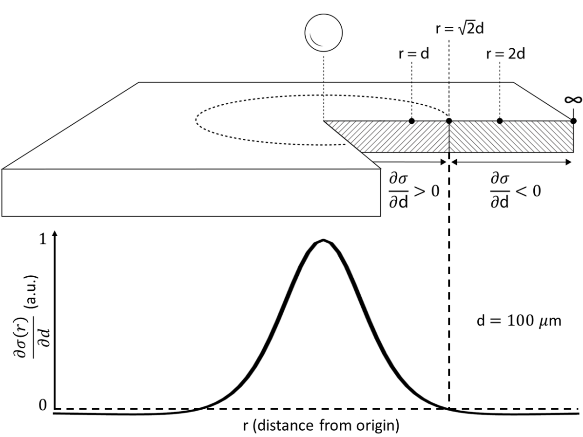
Figure 2: Regions of interest. (Top) The round ball represents a positively charged ion. When the ion moves away from the plane, negative charges induced below the ion in the region $r<\sqrt{2}$ become dispersed and exit the region as they move towards $r=\infty$. The region $r<\sqrt{2}$ becomes more positive, meaning $\frac{\partial\sigma}{\partial d}>0$. In contrast, the region $r>\sqrt{2}$ gains negative charges from the region $r<\sqrt{2}$, so it becomes more negative, and $\frac{\partial\sigma}{\partial d}<0$. (Bottom) A plot of the change in surface-charge density as the ion moves farther from the surface, $\frac{\partial\sigma}{\partial d}$ (in arbitrary units), as a function of distance $r$ from the origin.

Several relevant quantities include:

1. The potential $V(x,y,z)$

2. The surface-charge density $\sigma$

3. The variation of $\sigma$ with distance $d$ from the
   surface, $\frac{\partial\sigma}{\partial d}$

4. The sign and value of $\frac{\partial\sigma}{\partial d}$ at various places

The significance of these quantities applies to a broad range of experimental configurations. While specific values may vary from one experimental setup to the next, the main physics will generally remain the same.

I.2 Induced charge and induced current

With the general features of the system outlined, we turn to calculating quantitative values relevant to designing an experiment. First, we look at the total charge which flows into and out of a given region of the conducting plane, during each oscillation of the particle. Specifically, we are interested in the disk-like region defined by the radius $r=\sqrt{2}d$. Measuring the total charge which flows into/out of this region when the particle oscillates gives the maximum electrical current which can be channeled, since adding the change in charge outside of $r=\sqrt{2}d$ would mean adding a contribution of opposite sign.

I.2.1 The total charge flow into / out of a given region over each oscillation of the particle

We begin by looking at how the surface-charge density $\sigma$ changes at a single point, $\frac{\partial\sigma}{\partial d}|_{r,\phi}$ , when the particle oscillates. This expression can then be integrated over a surface area to get the total charge flow into/out of a given region. Referring to Figure 1, let the amplitude of oscillation of a charged particle be denoted by $b_{\mathrm{o}}$. In typical ion-trap conditions, for an ion cooled near the ground state the total displacement of the ion, $2b_{\mathrm{o}}$, is on the order of a few tens of nanometers Daniilidis and Häffner (2013). The distance $d$ between the ion and the trap electrodes (or conducting surface) is on the order of fifty to two hundred micrometers. Thus, it is reasonable to assume $d>>2b_{\mathrm{o}}$,  and therefore that $\frac{\partial\sigma}{\partial d}$ is approximately constant over $2b_{\mathrm{o}}$, which is to say $\frac{\partial\sigma}{\partial d}\sim\frac{\partial\sigma}{\partial d}\big{|}_{d=d_{\mathrm{eq.}}}$ where $d_{\mathrm{eq.}}$ is the equilibrium distance between the ion and the conducting surface, around which the ion oscillates. Thus, $\frac{\partial\sigma}{\partial d}\sim\mathrm{constant}=A\frac{r^{2}-2d_{\mathrm{eq.}}^{2}}{(r^{2}+d_{\mathrm{eq.}}^{2})^{5/2}}$  , which is equivalent to the linear relationship:

$$\Delta\sigma=\left(A\frac{r^{2}-2d_{\mathrm{eq.}}^{2}}{(r^{2}+d_{\mathrm{eq.}}^{2})^{5/2}}\right)\Delta d$$ (12)

The variation of the ion’s position as it oscillates can be described as sinusoidal, with an amplitude $b(t)=b_{\mathrm{o}}\sin{\omega t}$. Therefore, integrating equation (12) with respect to $d$ gives:

$$\sigma=\left(A\frac{r^{2}-2d_{\mathrm{eq.}}^{2}}{(r^{2}+d_{\mathrm{eq.}}^{2})^{5/2}}\right)b(t)+\sigma_{0}~{},$$ (13)

where $\sigma_{0}=A\frac{d_{\mathrm{eq.}}}{(r^{2}+{d_{\mathrm{eq.}}}^{2})^{3/2}}$ (equation (3) evaluated at $d_{\mathrm{eq.}}$). Using the expression for $\sigma$ linearized over $d$, which is effectively what has been done to get equation (13), it is now possible to evaluate the total charge that flows into or out of a given region, as the particle oscillates. First, $\sigma$ is integrated over some surface to get the total charge enclosed on that surface. Second, the result is evaluated once when the particle is at its farthest from the surface, and once again when the particle is at its closest to the surface. Then the difference is taken.

Integrating $\sigma$ over a disk of surface-area extending outwards from $r^{\prime}=0$ to $r^{\prime}=r$ (the ’primes’ have been added to distinguish between the evaluated and non-evaluated, integrated expression of $\sigma$) gives:

$$Q= \int_{\phi=0}^{\phi=2\pi}\int_{r^{\prime}=0}^{r^{\prime}=r}A\Bigg{(}\frac{r^{\prime 2}-2d_{\mathrm{eq.}}^{2}}{(r^{\prime 2}+d_{\mathrm{eq.}}^{2})^{5/2}}b_{\mathrm{o}}\sin{\omega t}$$ (14)

$$+~{}\frac{d_{\mathrm{eq.}}}{(r^{\prime 2}+{d_{\mathrm{eq.}}}^{2})^{3/2}}\Bigg{)}r^{\prime}dr^{\prime}d\phi~{}.$$

After the integral is calculated, evaluating the resulting expression when the particle is closest to the surface ($\sin{\omega t}=-1$), and again when it is farthest from the surface ($\sin{\omega t}=+1$), and taking the difference, gives:

$$Q_{\mathrm{transf.}}=\frac{2qr^{2}b_{\mathrm{o}}}{(r^{2}+{d_{\mathrm{eq.}}}^{2})^{3/2}}$$ (15)

This is the total change in charge contained within a disk-like region centered around $r=0$, when an ion above an infinite plane moves from $d_{\mathrm{eq.}}-b_{\mathrm{o}}$ to $d_{\mathrm{eq.}}+b_{\mathrm{o}}$. It should be noted that linearizing the surface charge with respect to $d$ to get equation (13) comes at a cost; in the limit $d\gg r$, the linearized surface-charge density in equation (13) dies off with $1/d^{3}$ as the ion moves farther away from the surface. However, in the non-linearized case, equation (3) dies off with $1/d^{2}$. The price of mathematical simplicity is a sacrifice in physical generality—a point which will re-appear as a footnote in section (II.5), and in appendix F. We can evaluate expression (15) for realistic values. For quantum computing applications, a trapped ion is typically cooled to near its motional ground state. For an ion behaving as a quantum harmonic oscillator in its ground state, the amplitude of oscillation (really the standard deviation of the position) around the minimum potential energy is given by:

$$b_{\mathrm{o}}=(\langle 0|z^{2}|0\rangle)^{\frac{1}{2}}=(\hbar/2m\omega)^{\frac{1}{2}}~{},$$ (16)

where $z$ is the position operator for displacement in the vertical direction, $\hbar=h/\left(2\pi\right)$ is the reduced Plank’s constant, $m$ is the mass of the charged particle, and $\omega=2\pi f$ is the angular frequency along the axis of the harmonic potential. This is defined to be one half the total spread of the zero-point wavefunction. Substituting equation (16) into equation (15) gives

$$Q_{\mathrm{transf.}}=\frac{2qr^{2}}{(r^{2}+{d_{\mathrm{eq.}}}^{2})^{3/2}}\left(\frac{h}{8\pi^{2}mf}\right)^{1/2}~{}.$$ (17)

Evaluating equation (16) for the mass of a ${}^{9}\mathrm{Be}^{+}$ ion $m=1.5\times 10^{-26}~{}$kg, and $f=5~{}$MHz gives the spread of the zero-point wavefunction $2b_{\mathrm{o}}\sim 20~{}\times 10^{-9}~{}$m. Evaluating equation (17) for $q=-e=1.6\times 10^{-19}~{}\mathrm{C}~{}$, $d_{\mathrm{eq.}}=50\times 10^{-6}~{}\mathrm{m}~{}$, $r=\sqrt{2}d_{\mathrm{eq.}}$, and $2b_{\mathrm{o}}\sim 20~{}\times 10^{-9}~{}\mathrm{m}$, we find: $Q_{\mathrm{transf.}}=2.6\times 10^{-23}~{}\mathrm{C}$. Note that $Q_{\mathrm{transf.}}$ is maximized for $r=\sqrt{2}d_{\mathrm{eq.}}$,  as one might expect from equation (7).

I.2.2 Induced current

In the previous section (I.2.1) we calculated the positive charge flow into (really the electron flow out of) a disk-like region centered around $r=0$, when a positive ion moves a small distance away from a grounded conducting plane. However, this calculation does not specify where the charge flows from, or to, as it re-distributes to reach the new equilibrium configuration. For instance, the charge could flow along the surface of the conductor in the in-plane direction, or vertically ’upwards’ $/$ ’downwards’ through the thickness of the infinite plane. While this is not relevant when considering equilibrium configurations, the question becomes essential if one aims to channel the charge flow to another ion or another type of qubit. For example, if a measuring device is connected to a region of the conducting plane right below the ion (see Figure 3), what is to prevent the induced currents from flowing sideways along the surface of the plane to re-equilibrate, rather than through the measuring device? The answer is, nothing.

Therefore, one must ensure that current-flow is properly channeled. This can be done by making the relative resistance through the wire to ground, or to another ion, much less than the resistance of any other path to re-equilibration. In the example of an infinite plane, such a configuration can be implemented by cutting a groove around the disk-shaped region beneath the ion, or otherwise insulating such a disk-shaped region from the rest of the conducting plane (Figure 3). If a conducting wire is connected from the disk to ground, the only way for charge to re-equilibrate is through the wire. As an alternative to cutting a groove, the rest of the infinite plane could be removed entirely. Although from an experimental standpoint this may be an improvement, it would also affect the potential between the ion and the disk-shaped conducting surface, meaning all of the equations up until now would have to be revised. For the sake of developing a model with a potential which is easily tractable using analytical expressions, we will continue to assume an infinite plane with a thin circular groove cut out around a central disk. Practical implications of this assumption are discussed in sections II.3 and V.

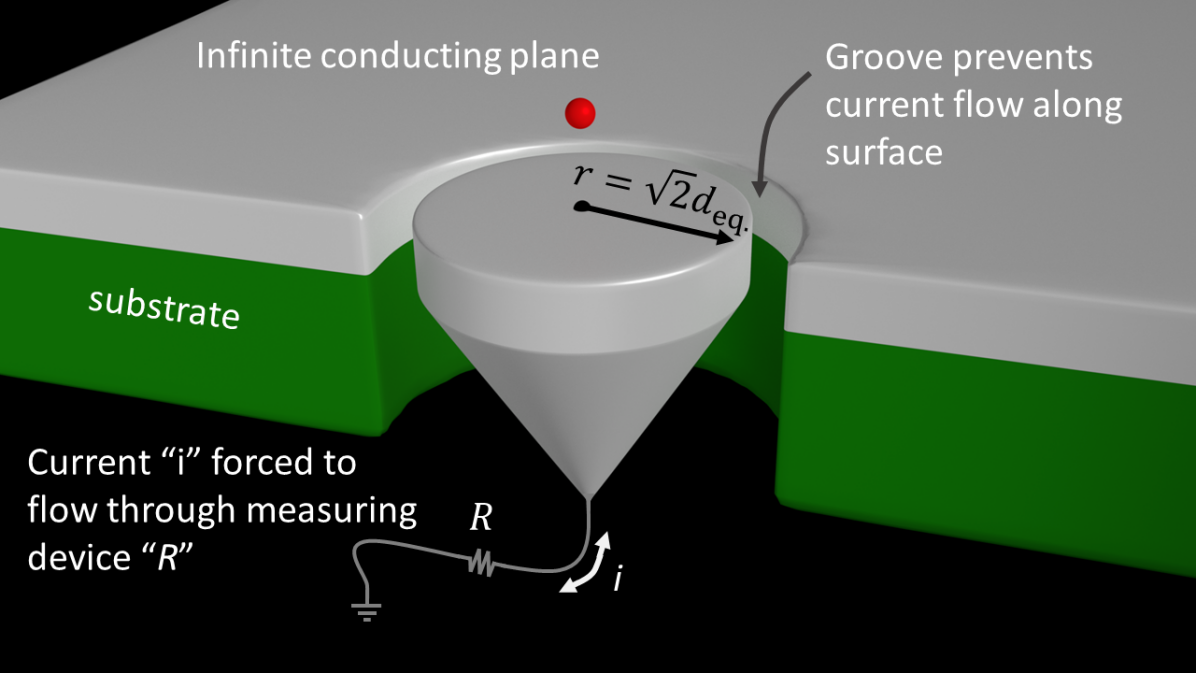
Figure 3: Pickup disk isolated by a groove to channel charge flow. The red circle represents a trapped ion. If the ion oscillates above a continuous infinite conducting plane, the induced charge-imbalance can re-equilibrate by flowing in the in-plane direction. Cutting a groove prevents this, and allows the induced current to be channeled.

With the current properly channeled and using the result from section (I.2.1), assuming all of the charge $Q_{\mathrm{transf.}}$ flows to ground in the time of one half-cycle, the time-averaged current throughout each $1/2$-cycle is:

$$Q_{\mathrm{transf.}}=I_{\mathrm{av}.}t\quad\Rightarrow\quad(2f)\times Q_{\mathrm{transf.}}=I_{\mathrm{av}.}~{},$$ (18)

where $f$ is the frequency of oscillation of the ion, typically in the range of $100~{}$kHz to $10~{}$MHz. Here, as before, we will assume $f=5~{}$MHz. If the trap potential is approximately harmonic, then the ion’s motion is approximately sinusoidal. For a sinusoidal current, the value $I_{\mathrm{av}.}$ is also referred to as $I_{\mathrm{rav}}$, for ’rectified average current’. Thus Young et al. (2007a): $I_{\mathrm{av}.}=I_{\mathrm{rav}}=\frac{2}{\pi}I_{\mathrm{max}}\sim 1.3\times 10^{-16}~{}\mathrm{A}$, and $I_{\mathrm{max}}\sim 2.0\times 10^{-16}~{}\mathrm{A}$. It should be highlighted that when calculating $I_{\mathrm{av}.}$ we assume all of the charge $Q_{\mathrm{transf.}}$ has time to flow to ground in one half-cycle. This assumption is only valid if the system is designed such that it is true, meaning the resistance $R$ is small enough, for a given capacitance of the disk. To maximize the current, the optimal radius of the disk is the same radius that maximizes $Q_{\mathrm{transf.}}$, $r=\sqrt{2}d_{\mathrm{eq.}}$. This radius can be used to calculate a capacitance for the disk, $C_{\mathrm{d}}=8\epsilon_{\mathrm{o}}r$, where $\epsilon_{\mathrm{o}}$ is the permittivity of free space. In section II.2, however, we will find that the coupling strength between two ions, ion#1 and ion#2, interacting via a conducting wire is maximized for a different radius, $r=d_{\mathrm{eq.}}/\sqrt{2}~{}$. For the following section we borrow the result from section II.2 to calculate a bound on the resistance $R$, using the model of a pickup disk attached to ground.

I.3 A constraint on the resistance

The assumption that all of the charge $Q_{\mathrm{transf.}}$ flows through the wire in the time of one half-oscillation of the ion places an upper-bound on the resistance $R$ of the wire. Since $Q_{\mathrm{transf.}}$ is confined to a disk of finite volume, the mutual repulsion of charges within the disk creates a potential associated with the disk itself. Intuitively, the greater the number of charges confined to a given volume (or surface, which is where the charges end up in a conductor), the greater the potential of that volume or surface. The ratio of the amount of charge confined on an object, to that object’s potential relative to ground, is an object’s self-capacitance. Figure (4) (left side) shows a disk where $Q_{\mathrm{transf.}}$ could be confined, resulting in a potential relative to ground, where the net charge-density is taken to be zero. The disk is connected to ground through a resistor, which represents the finite resistance of any real conducting wire.

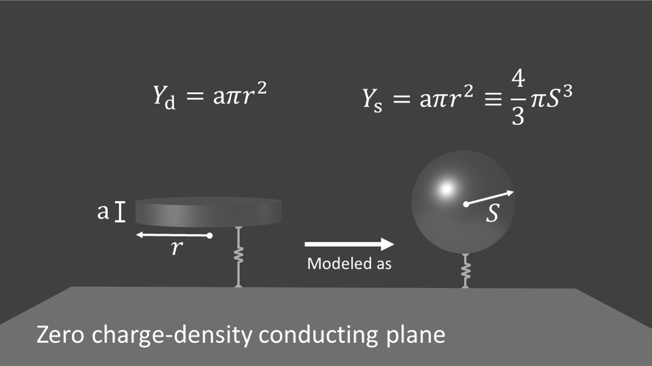
Figure 4: Charge draining from a disk or a sphere. Charge placed on a thin disk connected to ground drains off at a certain rate. Charge placed on a sphere with the same volume as the disk drains off more quickly; a sphere minimizes the distance between charges and increases their mutual repulsion.

To find the upper bound on $R$ we can use one of two approaches. Both approaches use the self-capacitance of the disk, $C_{\mathrm{d}}$, and the fixed time $T/2$ imposed by the period of oscillation of an ion in a trap, to calculate the maximum resistance $R$ which still allows all of the charge to drain to ground. The geometry of an object influences its self-capacitance; hence, the choice of model has a significant impact on the resulting range of acceptable $R$ values. For the two models considered here, a thin disk and a sphere, the self-capacitances are given by $C_{\mathrm{d}}\approx 8\epsilon_{\mathrm{o}}r$, and $C_{\mathrm{s}}=4\pi\epsilon_{\mathrm{o}}S$, respectively. $\epsilon_{\mathrm{o}}$ is the vacuum permittivity, $r$ is the radius of the disk, and $S$ is the radius of the sphere. The first approach to finding the upper bound on $R$ is to recognize that a capacitor connected through a resistor to ground is a low-pass filter. A low-pass filter has a cutoff frequency $\frac{1}{T}=f_{\mathrm{c}}=\frac{1}{2\pi RC}$. Below this frequency the signal is propagated, so rearranging gives the constraint $R<\frac{1}{2\pi f_{\mathrm{c}}C}$, where $C$ is the capacitance and $R$ is the resistance through which the capacitor drains to ground. The second approach is to use the capacitor discharge equation $V(t)=V_{0}e^{-t/\left(CR\right)}$, where $V(t)$ is the voltage after a time $t$, $V_{0}$ is the initial voltage, $C$ is the capacitance, and $R$ is the resistance through which the capacitor drains to ground. This equation is valid for both self-capacitance and mutual capacitance. Solving for $R$ gives

$$R=\frac{t}{C\ln{\left(V_{0}/V_{f}\right)}}~{},$$ (19)

where we changed the notation $V(t)$ to $V_{f}$, for ”final” voltage. We can evaluate equation (19) for the capacitance $C_{\mathrm{d}}$ of a thin disk. The distance $d_{\mathrm{eq.}}=50~{}\mu$m, which determines the optimum radius $r=d_{\mathrm{eq.}}/\sqrt{2}~{}$, determines the capacitance $C_{\mathrm{d}}~{}$, and using $f=5~{}$MHz, $t=1/\left(2f\right)$, and letting $V_{0}/V_{f}=10$ yields $R_{\mathrm{disk}}\sim 17~{}\mathrm{M}\Omega$. Next, we evaluate equation (19) for the capacitance $C_{\mathrm{s}}$ of a spherical conductor which has the same volume as the thin disk. The volume of a disk with finite thickness ”$\mathrm{a}$” is $Y_{\mathrm{d}}=\mathrm{a}\pi r^{2}$, and the volume of a sphere is $Y_{\mathrm{s}}=\frac{4}{3}\pi S^{3}$. Imposing $Y_{\mathrm{s}}=Y_{\mathrm{d}}$ gives $S=(\frac{3}{4\pi}\left(\mathrm{a}\pi r^{2}\right))^{1/3}$. Thus, $C_{\mathrm{s}}=4\pi\epsilon_{\mathrm{o}}(\frac{3}{4\pi}\left(\mathrm{a}\pi r^{2}\right))^{1/3}$. With $\mathrm{a}=1~{}\mu$m, $R_{\mathrm{Sphere}}\sim 40~{}\mathrm{M}\Omega$.

The maximum allowable value of $R$ calculated for the thin disk model is less than the maximum resistance allowed by the spherical volume model, which agrees with intuition. If charges are confined to the surface of a sphere, the average distance between them is minimized compared to if the charges are on the surface of any other shape which has the same volume, and hence on average they experience greater mutual repulsion. In general, the bound on $R$ can be expressed as a function $R\leq g\left(f,d_{\mathrm{eq.}},\mathrm{a}\right)$, which is the notation used in Table 6.

The self-capacitance of an object may change in a dynamical regime, if the skin depth at a given frequency approaches the dimension of the object. For a trapped ion oscillating at $5~{}$MHz, the skin-depth is on the order of $\delta\sim 30~{}\mu$m richard.ness@nessengr.com . This is likely greater than or comparable to the thickness of the pickup disk, which a priori could be of similar thickness to the trap electrodes, in the range $\mathrm{a}\sim 100~{}$nm to $\mathrm{a}\sim 10~{}\mu$m Labaziewicz et al. (2008); Hite et al. (2012); Daniilidis et al. (2014); Sedlacek et al. (2018a). Unfortunately, the electron configuration within the disk cannot be known without dedicated simulations, statistical mechanics calculations, or experiments specific to the thin-disk geometries in question. Hopefully, future studies will develop a fuller understanding of the dynamical behavior of the system.

This section ends with a remark on the interplay between the maximum resistance $R$ of the drainage wire (or measurement device), and the capacitance of the disk. We show above that the wire through which a current is channeled to another ion or a measurement device must not exceed certain upper bounds on $R$. In this description, as in figure 4, the coupling wire is represented by a wire with finite resistance, but zero capacitance. In reality, the coupling wire also has a finite capacitance. To avoid the wire absorbing charge which flows away from the disk and through the wire, which would diminish the signal, the capacitance and therefore the size of the wire should be as small as possible. Reducing the size of the wire increases its resistance. This trade-off seems potentially problematic. In appendix E we show that resistances for the wire sizes envisioned are well below the bound imposed by the capacitor discharge equation. In sections III.1, IV.4, and appendix E we discuss other limitations on the maximum resistance, related to thermal noise, which are stronger constraints.

II Coupling the motional states of two spatially distant charged particles, using an electrically floating wire

Table 1 lists parameter values which will often be used in the rest of this study. Where two notations are listed, both notations are used roughly interchangeably.

Table 1: Typical parameter values

Description	Variable	Value
Charge	$q_{\mathrm{c}}$	$e=1.6\times 10^{-19}~{}$C
Mass	$m$	$m_{{}_{{}^{9}\mathrm{Be}^{+}}}=1.5\times 10^{-26}~{}$kg
Dist. btw’n ion & disk	$d~{}$, $d_{\mathrm{eq.}}$	$50~{}\times 10^{-6}~{}$m
Radius of disk	$r~{}$, $r_{\mathrm{disk}}$	$d_{\mathrm{eq.}}/\sqrt{2}$
Length of wire	$l_{\mathrm{w}}~{}$, $l_{\mathrm{wire}}~{}$	$0.01~{}$m
Wire radius	$a$	$10~{}\times 10^{-6}~{}$m
Motional mode freq. rng.	$\Delta f$	$500~{}$Hz
Secular frequency	$f$	$5\times 10^{6}~{}$Hz
Temperature	$T$	$10~{}$K
Resistance	$R$	$0.001~{}\Omega$ or $0.0001~{}\Omega$

II.1 The physical model: differences and similarities with the ”grounded-disk” model

In the first part of this study, we considered a disk-like pickup electrode connected to ground via a wire. In what follows, the pickup electrode is instead connected to an electrically-floating wire, which carries the signal to a second ’transmitter’ disk placed at some distant location. The surface of the transmitter disk, referred to as disk2, also lies in the plane of the ground-plane, and is positioned below a second trapped ion, ion#2 (Figure 5). This new configuration is different from the pick-up disk connected to ground. To give an example, since the system is not grounded, when ion#1 moves closer to disk1, any charge that moves onto disk1 must come at the expense of charge on disk2. Despite differences, the setup bears an important calculational similarity to the configuration studied in section I. We will take advantage of this and use results from section I to help characterize the system of two ions coupled by a wire. This section is dedicated to deriving the strength of the coupling interaction between two trapped ions in separate traps.

Before beginning, we develop an intuitive picture of the mechanics of the system. Suppose ion#1 moves from its most distant position, to its closest position, relative to disk1. If the disk were initially grounded, an amount of charge $-~{}Q_{\mathrm{transf.}}$ would be drawn from ground and rise up onto disk1. However, since the ”floating-wire-and-disks” system is not grounded, if $-~{}Q_{1}$ comes up onto disk1, it must be at the expense of a corresponding $+~{}Q_{1}$ which develops on disk2, beneath ion#2 (assuming the intervening wire has zero capacitance). If ion#2 is at an equilibrium position $d_{\mathrm{eq.2}}$, now it will be repelled by the charge $+~{}Q_{1}$ beneath it, until it reaches a new equilibrium position, at a distance farther away from disk2. Thus, before ion#2 moves up (farther away), it experiences a potential across the distance from $d^{i}_{\mathrm{eq.2}}$ to $d^{ii}_{\mathrm{eq.2}}$. In principle, this potential could be calculated—in practice, the coupling between ion#1 and ion#2 is calculated directly from the change in the electric field.

II.2 Contributions to the potential

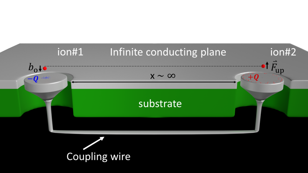
Figure 5: Ion#1 coupled to ion#2 using two conducting disks and a connecting wire. The two red dots represent positively-charged ions in separate traps. When ion#1 on the left moves downwards a distance $b_{\mathrm{o}}$ it induces charge $-Q$ on disk1. A corresponding positive charge $+Q$ is induced on disk2, which exerts a force $\vec{F}_{\mathrm{up}}$ on ion#2. The distance $x\sim\infty$ indicates the separation between ion#1 and ion#2 (about $0.1~{}$cm to $1~{}$cm) is much larger than all other characteristic dimensions of the system, such as the disk radii ($r\sim d_{\mathrm{eq.}}\sim 200~{}\mu$m).

Due to the symmetry of the setup, we only need to consider one of the two regions in figure 5. To maintain the approximation that the potential is described by two disks surrounded by an infinite plane, the connecting wire is illustrated as going down and running beneath the infinite grounded conducting plane. This reduces the chance that the wire itself disturbs the potential. We choose to look at the region above pick-up disk2 (henceforth disk2). There are four main contributions to the potential above disk2. (A possible 5th term describing a fixed bias-voltage is omitted from equation (20)):

$$V_{\infty 2}=V_{\mathrm{ion\#2}}+V^{\mathrm{induced~{}by~{}ion2}}_{\mathrm{disk2~{}+~{}\infty plane2}}$$

$$~{}~{}~{}~{}~{}~{}~{}~{}~{}~{}~{}~{}~{}~{}~{}~{}~{}~{}~{}~{}+~{}V^{\mathrm{induced~{}by~{}ion1}}_{\mathrm{disk2~{}+~{}\infty plane2}}+V_{\mathrm{rf-trap}}$$ (20)

Let’s consider these contributions one at a time. The first contribution, $V_{\mathrm{ion\#2}}$, is the potential produced by ion#2 itself. This is given by the expression:

$$V_{\mathrm{ion\#2}}=\frac{1}{4\pi\epsilon_{\mathrm{o}}}\left[\frac{q_{\mathrm{c}}}{\sqrt{r^{2}_{2}+(d_{\mathrm{eq.}2}-z_{2})^{2}}}\right]~{},$$ (21)

where the origin of the coordinate system is taken to be the center of disk2, $d_{\mathrm{eq.}2}$ is the equilibrium height of ion#2, $r_{2}$ is the radial distance from the origin, at which the potential is evaluated, $z_{2}$ is the vertical distance from the origin, at which the potential is evaluated, and $q_{\mathrm{c}}$ is the charge of ion#2.

The second contribution, $V^{\mathrm{induced~{}by~{}ion2}}_{\mathrm{disk2~{}+~{}\infty~{}plane2}}$, or in more compact notation $V^{\mathrm{i2}}_{\mathrm{d\&p2}}$, comes from the surface-charge which is induced by ion#2, on (disk2 + $\infty$ plane2). We can identify this contribution by taking the full potential (equation 1) and subtracting $V_{\mathrm{ion\#2}}$, which gives, after converting to cylindrical coordinates:

$$V^{\mathrm{i2}}_{\mathrm{d\&p2}}=\frac{1}{4\pi\epsilon_{\mathrm{o}}}\left[-\frac{q_{\mathrm{c}}}{\sqrt{r^{2}_{2}+(z_{2}+d_{\mathrm{eq.}2})^{2}}}\right]$$ (22)

The potential produced by this induced charge is of opposite sign from the potential produced by the ion, since the induced charge is of opposite sign from the charge of the ion.

The third contribution is from the surface-charge induced by ion#1, on (disk2 + $\infty$ plane2). We call this contribution $V^{\mathrm{induced~{}by~{}ion1}}_{\mathrm{disk2~{}+~{}\infty plane2}}$, or more compactly $V^{\mathrm{i1}}_{\mathrm{d\&p2}}$. To visualize the source of $V^{\mathrm{i1}}_{\mathrm{d\&p2}}$, consider figure 5. Assume that all of the surfaces in the system (disk1, disk2, both planes, and the connecting wire) are initially grounded, at potential $V=0$. Additionally, suppose that ion#1 starts at a distance ${d_{\mathrm{eq.1}}+b_{\mathrm{o}}}$ above disk1. From previous calculations for a pick-up disk connected to ground in section I, when ion#1 moves from ${d_{\mathrm{eq.1}}+b_{\mathrm{o}}}$ to ${d_{\mathrm{eq.1}}-b_{\mathrm{o}}}$, disk#1 will try to draw an amount of charge $-Q_{\mathrm{transf.}}$ upwards onto the surface of disk1. This would re-establish the equilibrium configuration of (disk1 + $\infty$ plane1). However, any charge $-Q_{1}$ drawn onto disk1 must come at the expense of inducing a corresponding charge $+Q_{1}$ on disk2. Thus, as ion#1 oscillates, it induces a periodically oscillating charge on disk 2. This creates an alternating potential above disk2.

The fourth contribution to $V_{\infty 2}$ is $V_{\mathrm{rf-trap}}$. This contribution is assumed to be entirely independent of the positions $d_{\mathrm{eq.1}}$ and $d_{\mathrm{eq.}2}$ of the ions. It is provided by the trap electrodes using an external source, and is well approximated as a harmonic potential, though often with different ”spring constants” along different axes of the trap.

II.3 Calculating the coupling between ion $\#1$ and ion $\#2$

The interaction between ion#1 and ion#2 can be described by a coupling constant, $\gamma$. The coupling constant $\gamma$ may be thought of as the linear change in force on ion#2 when the distance between ion#1 and disk1 changes. There is also a linear change in the force on ion#1 when the distance between ion#2 and disk2 changes, so $\gamma$ contains two terms:

$$\gamma\equiv\frac{1}{2}\left[\frac{\partial}{\partial{b_{2}}}\left(-\vec{F_{1}}\right)+\frac{\partial}{\partial{b_{1}}}\left(-\vec{F_{2}}\right)\right]~{},$$ (23)

where $b_{2}$ and $b_{1}$ represent the instantaneous displacement of ion#2 and ion#1 away from their equilibrium positions, as they oscillate. The factor of $\frac{1}{2}$ is to avoid double-counting the energy, as stated in Daniilidis et al. (2009). Equation (23) amounts to averaging the effect of ion#1 on ion#2 when ion#1 moves, with the effect of ion#2 on ion#1 when ion#2 moves, and defining this average to be the coupling strength. It is roughly equivalent to the definition $\gamma\equiv\frac{1}{2}\left[\frac{\partial^{2}\left(U_{1}+U_{2}\right)}{\partial{b_{1}}\partial{b_{2}}}\right]$, used in reference Daniilidis et al. (2009), where $U_{1}$ and $U_{2}$ are the total energy of ion#1 and ion#2 (the total potential they feel, times the charge of the ion $e$). Exact equivalence occurs if $U_{1}$ has continuous second partial derivatives at all points, which according to Schwarz’s theorem guarantees that $\frac{\partial^{2}\left(U_{1}\right)}{\partial b_{1}\partial{b_{2}}}=\frac{\partial^{2}\left(U_{1}\right)}{\partial b_{2}\partial{b_{1}}}$. The first term in (23) describes how much the force on ion#1 changes, for a small change in the position of ion#2. The second term in (23) describes how much the force on ion#2 changes when the position of ion#1 changes by a small amount. Another way to think of $\gamma$ is as the ’spring constant’ $k$ which expresses the rigidity of the connection between the two ions. This is illustrated most clearly by re-casting the relationship between the displacement of one ion, and the force felt by the other ion: $\vec{F}_{2}=k\vec{b}_{1}\Rightarrow\frac{\partial(\vec{F}_{2})}{\partial{b_{1}}}=k$.

One might wonder why the partial derivatives are not taken with respect to $d_{\mathrm{eq.1}}$ and $d_{\mathrm{eq.2}}$, and why one should not calculate $\frac{\partial\vec{F}_{2}}{\partial d_{\mathrm{eq.1}}}$ and $\frac{\partial\vec{F}_{1}}{\partial d_{\mathrm{eq.2}}}$ , rather than $\frac{\partial\vec{F}_{2}}{\partial b_{1}}$ and $\frac{\partial\vec{F}_{1}}{\partial b_{2}}$. Indeed, the total change in force depends on both the change in $d_{\mathrm{eq.1}}$  plus the instantaneous change in $b_{1}$. However, the contribution from $\frac{\partial\vec{F}_{2}}{\partial\vec{d}_{\mathrm{eq.1}}}$ is effectively negligible in the overall coupling constant $\gamma_{\mathrm{tot.}}=\gamma_{b}+\gamma_{d_{\mathrm{eq.}}}$. Over the course of one oscillation of ion#1 or ion#2, there should be virtually no change in the average distance of the ion $d_{\mathrm{eq.1}}$ or $d_{\mathrm{eq.2}}$, (for example due to drifts in the trapping potential), but there will be a change in the position of the ion due to its short time-scale oscillations. Thus, over a given time $t\sim 1~{}\mu$s ,  $\Delta d_{\mathrm{eq.1}}\approx\Delta d_{\mathrm{eq.2}}\ll\Delta b_{1}\approx\Delta b_{2}$. This means during one oscillation, $\vec{F_{2}}^{\mathrm{tot}}=k_{b}\vec{\Delta b}+k_{d_{\mathrm{eq.}}}\vec{\Delta d_{\mathrm{eq.}}}\approx k_{b}\vec{\Delta b}$. What has been referred to as $\gamma$ above should in fact more accurately be referred to as $\gamma_{b}$. However, we continue to describe this quantity simply as $\gamma$ for ease of notation, and because there will be no ambiguity moving forward.

Equation (23) shows that for ion#2 to contribute to $\gamma$, the force $\vec{F}_{2}$ on ion#2 must depend on $b_{1}$, the displacement of ion#1 towards or away from disk#1. Otherwise, the partial derivative with respect to $b_{1}$ yields zero. Similarly, the force on ion#1 must depend on $b_{2}$. Referring to section (II.2), among the four contributions to $V_{\infty 2}$ (eq. (20)) for the potential in region#2, the first, second, and fourth contributions do not depend on $b_{1}$. Only the third term, $V^{\mathrm{i1}}_{\mathrm{d\&p2}}$, depends on both $b_{2}$ and $b_{1}$. Since $\vec{F_{2}}$ in equation (23) is the same as writing: ”the gradient with respect to $b_{2}$ of $\left(-qV_{\infty 2}~{}\right)$”, any terms in $V_{\infty 2}$ which do not depend on $b_{1}$, will correspond to terms in $\vec{F_{2}}$ which also do not depend on $b_{1}$. Terms $1$, $2$, and $4$ in eq. (20) can therefore be ignored for the purpose of calculating $\gamma$:

$$V_{\infty 2}~{}= ~{}\cancel{V_{\mathrm{ion\#2}}}+\cancel{V^{\mathrm{induced~{}by~{}ion2}}_{\mathrm{disk2~{}+\infty plane2}}}$$ (24)

$$+~{}V^{\mathrm{induced~{}by~{}ion1}}_{\mathrm{disk2~{}+~{}\infty plane2}}+\cancel{V_{\mathrm{rf-trap}}}~{}.$$

Thus, calculating $\gamma$ reduces to finding $V^{\mathrm{i1}}_{\mathrm{d\&p2}}$.

To find $V^{\mathrm{i1}}_{\mathrm{d\&p2}}$ we consider the electric field produced above disk2. Indeed, the electric field is all that is needed to calculate $\gamma$, because $\gamma$ can be directly calculated from the force $\vec{F}_{2}=q_{\mathrm{c}}\times\vec{E}_{2}$. The electric field produced by bringing an amount of charge $+~{}Q_{2}$ onto disk2 is found using the following reasoning. When the charges which make up $+~{}Q_{2}$ are placed on disk2, they spread out towards the edges of the disk as they try to move as far away from each other as possible. Their potential energy is minimized when they form a ring centered around the z-axis. This configuration is reached provided that the charges placed on disk2 are given enough time to redistribute and reach their equilibrium configuration. For our purposes, the condition is met so long as the charges re-distribute quickly compared to the time-period of one half-oscillation of the ion. The width of the resulting ring of charge is thin compared to the full radius of the disk, so we consider all of the charge to be distributed in a ring of radius $r_{\mathrm{disk}}$. (See proof in appendix A. The approximation becomes less valid for thinner disks.) Equation (25) describes the electric field along the z-axis, produced by a ring of charge centered around the z-axis and lying in a plane perpendicular to the z-axis Young et al. (2007b):

$$\vec{E}_{\infty 2}=\frac{1}{4\pi\epsilon_{\mathrm{o}}}{\frac{Q_{2}z}{\left(z^{2}+r^{2}\right)^{3/2}}}\hat{z}~{}.$$ (25)

Here, $z$ is the vertical distance from the plane of the ring, and $r$ is the radius of the ring. When evaluated at the position of ion#2, and for the radius of disk2, this gives:

$$\vec{E}_{\infty 2}= \frac{1}{4\pi\epsilon_{\mathrm{o}}}{\frac{Q_{2}d_{\mathrm{eq.2}}}{\left(d_{\mathrm{eq.2}}^{2}+r_{\mathrm{disk2}}^{2}\right)^{3/2}}}\hat{z}$$ (26)

$$~{}~{}~{}~{}~{}~{}~{}~{}~{}~{}~{}=\frac{1}{4\pi\epsilon_{\mathrm{o}}}{\frac{-Q_{1}d_{\mathrm{eq.2}}}{\left(d_{\mathrm{eq.2}}^{2}+r_{\mathrm{disk2}}^{2}\right)^{3/2}}}\hat{z}$$

On the right-hand side of expression (26),  $Q_{1}$ is related to the charge which is induced on disk1 by the displacement of ion#1; in other words, it is related to $Q_{\mathrm{transf.}}$. The second equality in expression (26) represents a strong assumption, that the charge which appears on disk2 due to ion#1 is exactly the same in magnitude, but opposite in sign from the charge induced on disk#1 by ion#1. This assumption is valid provided the amount of charge which accumulates in the wire and is subsequently given up by the wire during each oscillation of the ion is negligible compared to the total charge which is accumulated and given up by each of the disks. In other words, it is valid if the capacitance of the wire connecting disk1 and disk2 is negligible compared to the capacitances of disk1 and disk2. The assumption is lifted below with the introduction of a unitless coefficient $\zeta$, which not only relates $Q_{1}$ to $Q_{\mathrm{transf.}}$, but also accounts for a finite capacitance of the wire. For the illustrative case above, the second equality can be understood as representing a scenario in which disk1 and disk2 have equal capacitances, and the wire capacitance is zero. In such a situation, the equilibrium state is for each disk to carry an equal amount of the charge-imbalance resulting from the movement of ion#1 (see appendix B.1).

Given a known relationship between $Q_{\mathrm{transf.}}$ and $Q_{1}$, and a known relationship between $Q_{1}$ and $Q_{2}$ (see appendix B), the electric field may be rewritten by substituting in $Q_{2}=-\zeta Q_{\mathrm{transf.}}=-\zeta\frac{q_{\mathrm{c}}r^{2}b_{1}\left(t\right)}{(r^{2}+{d_{\mathrm{eq.}}}^{2})^{3/2}}$ . Here, the coefficient $\zeta$ is calculated in appendix B.3 (equation (77)), and the second equality comes from substituting in the explicit, unevaluated expression for $Q_{\mathrm{transf.}}$  (after calculating the integral in (14), but before equation (15)). Substituting $Q_{2}$ into equation (26), the electric field can be rewritten as

$$\vec{E}_{\infty 2}= \frac{1}{4\pi\epsilon_{\mathrm{o}}}{\frac{d_{\mathrm{eq.2}}}{\left(d_{\mathrm{eq.2}}^{2}+r_{\mathrm{disk2}}^{2}\right)^{3/2}}}$$ (27)

$$~{}~{}~{}~{}~{}~{}~{}~{}~{}~{}~{}~{}~{}~{}~{}~{}~{}\times\frac{-\zeta q_{\mathrm{c}}r_{\mathrm{disk1}}^{2}b_{1}\left(t\right)}{\left(r_{\mathrm{disk1}}^{2}+{d_{\mathrm{eq.1}}}^{2}\right)^{3/2}}\hat{z}~{}.$$

After multiplying the electric field by $q_{\mathrm{c}}$ we arrive at an expression for the upwards force $\vec{F_{2}}$ exerted on ion#2, which depends on $b_{1}$. From this, and an equivalent expression for the force $\vec{F_{1}}$ exerted on ion#1, one can calculate the coupling $\gamma$ (or at any rate, the $\hat{z}$ component of $\gamma$). Dropping the vector notation we have:

$$\gamma=\frac{1}{2}\left[\frac{\partial}{\partial{b_{2}}}(-F_{1})+\frac{\partial}{\partial{b_{1}}}(-F_{2})\right]~{},$$

therefore,

$$\gamma=\zeta\frac{1}{8\pi\epsilon_{\mathrm{o}}}{\frac{d_{\mathrm{eq.1}}}{\left(d_{\mathrm{eq.1}}^{2}+r_{\mathrm{disk1}}^{2}\right)^{3/2}}}{\frac{{q_{\mathrm{c}}}^{2}r_{\mathrm{disk2}}^{2}}{\left(r_{\mathrm{disk2}}^{2}+{d^{2}_{\mathrm{eq.2}}}\right)^{3/2}}}$$

$$+~{}\zeta\frac{1}{8\pi\epsilon_{\mathrm{o}}}{\frac{d_{\mathrm{eq.2}}}{\left(d_{\mathrm{eq.2}}^{2}+r_{\mathrm{disk2}}^{2}\right)^{3/2}}}{\frac{q^{2}_{\mathrm{c}}r_{\mathrm{disk1}}^{2}}{\left(r_{\mathrm{disk1}}^{2}+{d^{2}_{\mathrm{eq.1}}}\right)^{3/2}}}$$ (28)

The units of $\gamma$ are Newtons per meter, which corresponds to the force exerted on ion#2 (ion#1) for a given displacement of ion#1 (ion#2), similar to a standard spring constant.

It was mentioned earlier that charges placed on the flat conducting disk will naturally accumulate around the edges, forming a ring. What was not mentioned is that the positive charges in this ring induce a negative charge-density in the infinite plane around them, thus forming a second, negatively-charged ring. The second ring partially cancels out the electric field produced by the first ring, and reduces the strength of the coupling constant. We argue in appendix C that this second ring can be ignored, and the calculation of $\gamma$ above is sufficient.

II.4 Optimizing the coupling constant $\gamma$

The expression for gamma calculated in section II.3, (or appendix (82)), can be optimized as a function of the disk radii to maximize the coupling. Plugging in values for $d_{\mathrm{eq.1}},d_{\mathrm{eq.2}},q,\zeta,$ and $\epsilon_{\mathrm{o}}$ gives an expression $\gamma\left(r_{\mathrm{disk1}},r_{\mathrm{disk2}}\right)$. If one imposes that the coupling system should be symmetrical, $r_{\mathrm{disk1}}=r_{\mathrm{disk2}}=r$, $\zeta$ reduces to $\zeta=\frac{1}{2+C_{b}/C_{\mathrm{disk}}}$, where $C_{b}$ is the wire capacitance. Imposing $d_{\mathrm{eq.1}}=d_{\mathrm{eq.2}}=d$, and substituting in the explicit expression for the disk capacitance, $C_{\mathrm{d}}=8\epsilon_{\mathrm{o}}r$ from section I.2.2, gamma becomes simply $\gamma\left(r\right)$. Now, the optimization of $\gamma$ is an optimization of a function with only one independent variable, $r$,

$$\gamma=\frac{q^{2}_{\mathrm{c}}}{4\pi\epsilon_{\mathrm{o}}}\left(\frac{1}{2+\frac{C_{b}}{8\epsilon_{\mathrm{o}}r}}\right)\left(\frac{dr^{2}}{\left(d^{2}+r^{2}\right)^{3}}\right)\hat{z}~{}.$$ (29)

Unfortunately, maximizing the full expression for $\gamma$ by solving $\frac{\partial}{\partial r}\gamma\left(r\right)=0$ analytically, is not trivial. However, looking at the portion in the left-most parentheses of equation $\eqref{gamma_symm}$, which corresponds to the expression for $\zeta$ , we see that equation $\eqref{gamma_symm}$ can be simplified in the limit $2\gg\frac{C_{b}}{C_{\mathrm{disk}}}$. In this case, $\zeta=\frac{1}{2}$ which is independent of $r$. Optimizing the remaining portion of $\gamma$ one finds

$$\frac{\partial}{\partial r}\left(\frac{dr^{2}}{\left(d^{2}+r^{2}\right)^{3}}\right)=0\qquad\Rightarrow\qquad d=\sqrt{2}r$$ (30)

We can also consider the opposite limiting case, where the wire capacitance $C_{b}$ is much greater than the capacitance of the disks, $2\ll\frac{C_{b}}{C_{\mathrm{disk}}}$. For a disk capacitance $C_{\mathrm{d}}=8\epsilon_{\mathrm{o}}r$ it can be shown that $\gamma$ is optimized for $r_{\mathrm{opt.}}=d_{\mathrm{eq.}}$ (see appendix D). Thus, a general rule of thumb is $d_{\mathrm{eq.}}/\sqrt{2}\leq r_{\mathrm{opt.}}\leq d_{\mathrm{eq.}}$.

A priori, we still do not know whether in general, fully optimizing the expression in equation (29) could yield a significantly improved value of $r_{\mathrm{disk}}$. An exact numerical result for the optimal disk radius $r_{\mathrm{opt.}}$ can be found by plotting $\gamma\left(r\right)$ as a function of $r$, as shown in figure 6.

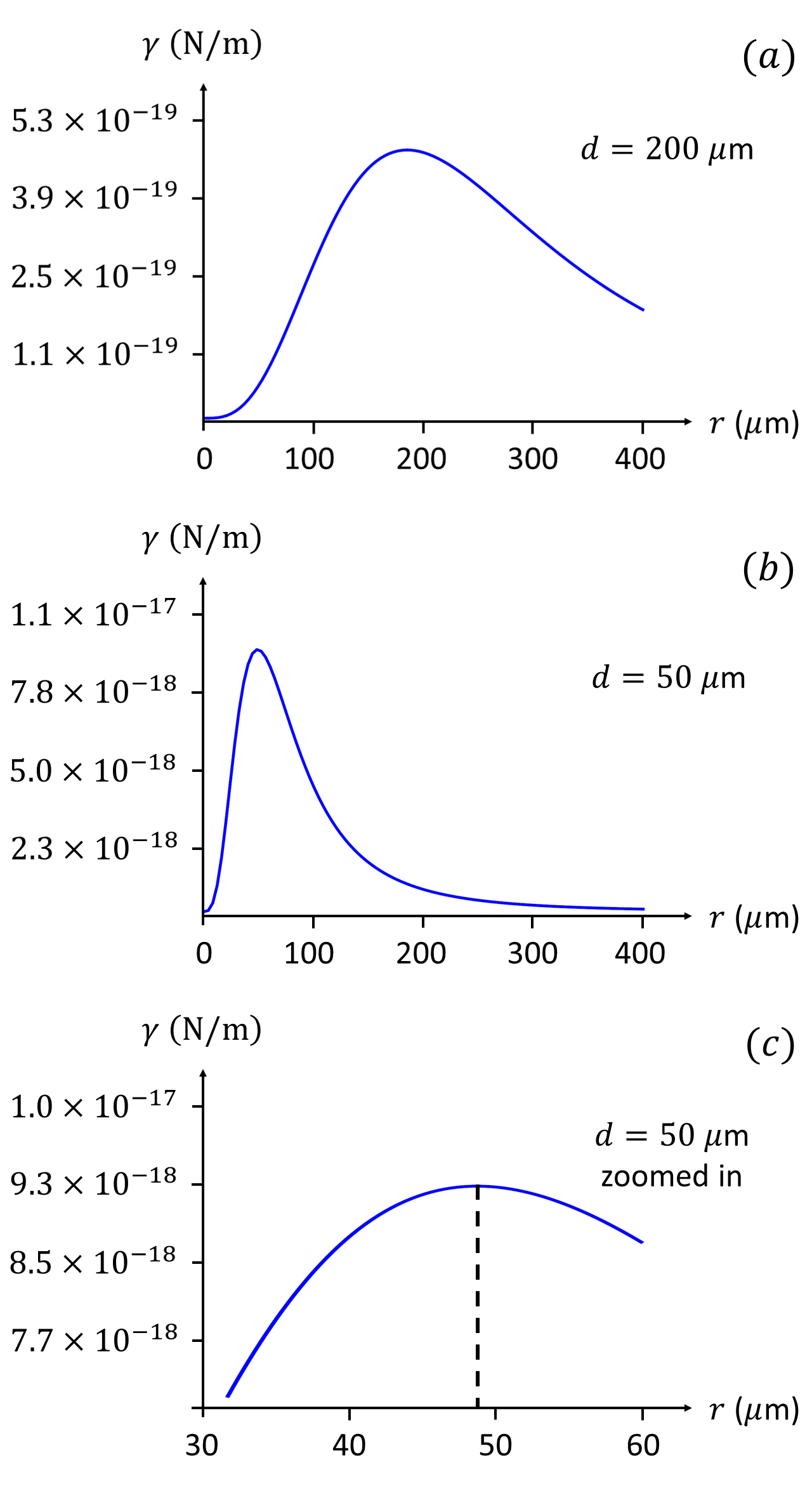
Figure 6: Coupling strength $\gamma$ (N/m) versus $r$ (micro-meters). ($a$) The coupling strength $\gamma$ is plotted as a function of the disk radius $r$, for a distance $d=200~{}\mu$m between the two ions and their respective coupling disks. The maximum coupling strength is $\gamma\sim 5\times 10^{-19}$ N/m. ($b$) The same as in ($a$) but for a distance $d=50~{}\mu$m between each ion and its coupling disk. The maximum coupling strength is $\gamma\sim 9\times 10^{-18}$ N/m. ($c$) the same plot as in ($b$), but zoomed in on the peak.

To plot $\gamma$, the capacitance $C_{b}$ is modeled as that of a thin cylindrical wire, $C_{b}=2\pi\epsilon_{\mathrm{o}}l_{\mathrm{wire}}/\mathrm{ln}\left(l_{\mathrm{wire}}/a\right)$, where $l_{\mathrm{wire}}$ is the length of the wire and $a$ is its radius. We let $a=10~{}\mu$m, and $l_{\mathrm{wire}}=1~{}$cm, which gives $C_{b}=8.0\times 10^{-14}~{}$F. For these parameter values, for two representative distances $d_{\mathrm{eq.}}=200~{}\mu$m and $d_{\mathrm{eq.}}=50~{}\mu$m, the ratios of wire capacitance to disk capacitance are $C_{b}/C_{\mathrm{disk}}=8$, and $C_{b}/C_{\mathrm{disk}}=32$, respectively. Both cases fall in the regime $2\ll\frac{C_{b}}{C_{\mathrm{disk}}}$, meaning we expect that $r_{\mathrm{opt.}}\sim d_{\mathrm{eq.}}$. This can be verified by looking at the numerical results. Figure 6 ($a$) shows the exact numerical result for $d=200~{}\mu$m is $r_{\mathrm{opt.}}\approx 180~{}\mu$m. Figure 6 ($b$) and ($c$) show the exact numerical result for $d=50~{}\mu$m is $r_{\mathrm{opt.}}\sim 48~{}\mu$m. We see that for the smaller distance, $d_{\mathrm{eq.}}=50~{}\mu$m, the numerical result $r_{\mathrm{opt.}}\approx 48~{}\mu$m is close to $r=d_{\mathrm{eq.}}$, confirming we are in the $2\ll\frac{C_{b}}{C_{\mathrm{disk}}}$ regime. For the larger distance $d_{\mathrm{eq.}}=200~{}\mu$m, the analytical result $r_{\mathrm{opt.}}\sim 180~{}\mu$m is slightly closer to $r_{\mathrm{opt.}}=d_{\mathrm{eq.}}/\sqrt{2}=140~{}\mu$m, which is the optimal value for the $2\gg\frac{C_{b}}{C_{\mathrm{disk}}}$ regime. Nevertheless, the setup is still closer to the $2\ll\frac{C_{b}}{C_{\mathrm{disk}}}$ regime.

Next, we compare numerically optimized results for $\gamma$ with values of $\gamma$ calculated for the $2\gg\frac{C_{b}}{C_{\mathrm{disk}}}$ regime, where $r_{\mathrm{opt.}}=d_{\mathrm{eq.}}/\sqrt{2}$, shown in table 2. Results are shown for two different values of the distance between the ion and the surface, $d_{\mathrm{eq.}}=200~{}\mu$m, and $d_{\mathrm{eq.}}=50~{}\mu$m. $\gamma$ is also given for two different wire lengths, $l_{\mathrm{wire}}=1$ cm, and $l_{\mathrm{wire}}=10$ cm. The wire radius is $a=10~{}\mu$m in all cases.

Table 2: Values of $\gamma_{\mathrm{opt.}}$

$\gamma_{\mathrm{opt.}}$ (in $\mathrm{N/m}~{},\mathrm{or}~{}\frac{\mathrm{kg\cdot m}}{\mathrm{s}^{2}}$)	$d_{\mathrm{eq.}}$	$l_{\mathrm{wire}}$
$4.2\times 10^{-19}$	$200~{}\mu$m	1  cm
$6.8\times 10^{-20}$	$200~{}\mu$m	10  cm
$8.0\times 10^{-18}$	$50~{}\mu$m	1  cm
$1.1\times 10^{-18}$	$50~{}\mu$m	10  cm

We focus on the value of $\gamma$ calculated for $d_{\mathrm{eq.}}=50~{}\mu$m and $l_{\mathrm{wire}}=1~{}$cm, $\gamma=8.0\times 10^{-18}$. This is slightly lower than the fully optimized value shown in the zoomed-in plot in figure 6, $\gamma\sim 9\times 10^{-18}$. However, the difference between the two values is small despite the fact that the disk radius is small, which increases sensitivity to changes in $r$. This shows that the rule of thumb $d_{\mathrm{eq.}}/\sqrt{2}\leq r_{\mathrm{opt.}}\leq d_{\mathrm{eq.}}$ optimizes $\gamma$ reasonably well even if one is not certain of the regime in which the setup operates.

II.5 Comparing results for different systems

The coupling strength derived using the pickup-disk system can be compared with results of other analyses for coupling systems using wire-type architectures. At least four distinct physical implementations have been considered in various studies:

1. Pickup disks linked by a wire (this work), and Zurita-Sánchez and Henkel (2008); Marzoli et al. (2009); Sorensen et al. (2004).

2. Rectangular pickup electrodes linked by a wire Liang and Ke-Lin (2010).

3. A straight suspended wire, with two trapped ions suspended below it Daniilidis et al. (2009).

4. Equivalent-circuit systems Heinzen and Wineland (1990); Daniilidis et al. (2009); Kotler et al. (2017); Rica et al. (2018); Bohman et al. (2018).

Table 3 shows the coupling constant $\gamma$ calculated based on several of these studies. The blue entries rely on an approach used by Zurita-Sánchez and Henkel (2008); Marzoli et al. (2009); Liang and Ke-Lin (2010) which is slightly different from the one used here, and the brown values rely on another, very different approach outlined in Wineland and Dehmelt (1975), used in one of two calculations in Daniilidis et al. (2009), and in Heinzen and Wineland (1990); Kotler et al. (2017); Rica et al. (2018); Bohman et al. (2018). Most of the studies in the first three implementations above are targeted towards charged particles trapped in rf traps (Paul traps), or Penning traps (in the case of references Zurita-Sánchez and Henkel (2008); Marzoli et al. (2009)). In Heinzen and Wineland (1990); Daniilidis et al. (2009); Kotler et al. (2017); Rica et al. (2018); Bohman et al. (2018) a trapped particle is modeled as a charge placed between two electrodes resembling plates of a parallel-plate capacitor. As the charged particle oscillates, it induces a current within the plates which form part of an equivalent lumped circuit element system that may be linked to another particle. This model, originally described in Wineland and Dehmelt (1975), has been shown to be inappropriate for calculating coupling constants Van Horne and Mukherjee (2020a). The corresponding results in brown are included in table 3 for context only.

For the four physical implementations above, calculations of the coupling strength in all listed references (except Sorensen et al. (2004)) rely on three general methods, described in the following works. 1) This work, and one calculation in Daniilidis et al. (2009), uses a piecewise description of the system to construct a global model. 2) Reference Zurita-Sánchez and Henkel (2008) formulates the system in terms of Green’s functions and uses these to derive results. 3) Reference Wineland and Dehmelt (1975) introduces an equivalent lumped circuit element model which is widely used (incorrectly) to calculate coupling strengths.

Table 3: Values of $\gamma$ for various systems

$\gamma$  (in $\mathrm{N/m}~{},\mathrm{or}~{}\frac{\mathrm{kg\cdot m}}{\mathrm{s}^{2}}$)	$d_{\mathrm{eq.}}=50~{}\mu\mathrm{m}$	$d_{\mathrm{eq.}}=200~{}\mu\mathrm{m}$
$\gamma_{\mathrm{V.~{}pickup-disk}}$	$8.0\times 10^{-18}$	$4.2\times 10^{-19}$
$\gamma_{\mathrm{D.~{}suspended-wire}}$	$7.5\times 10^{-18}$	$7.9\times 10^{-19}$
$\gamma_{\mathrm{Z.~{}transmission-line}}$	$1.5\times 10^{-17}$	$8.2\times 10^{-19}$
$\gamma_{\mathrm{Z.~{}rectangular-electrodes}}$	$3.0\times 10^{-19}$	$2.1\times 10^{-19}$
$\gamma_{\mathrm{W.~{}mass-spring,~{}pickup-disk}}$	$8.0\times 10^{-18}$	$8.1\times 10^{-19}$
$\gamma_{\mathrm{W.~{}mass-spring,~{}parallel~{}plate}}$	$3.0\times 10^{-17}$	$1.6\times 10^{-18}$
$\gamma_{\mathrm{W.~{}mass-spring,~{}suspended~{}wire}}$	$1.1\times 10^{-17}$	$1.8\times 10^{-18}$

In each of the systems in table 3, the total energy can be modeled as that of two harmonic oscillators, with an added linear coupling term. The coupling can be described using the analogy of a mass and spring system, where two masses $m_{1}$ and $m_{2}$ are attached to two walls by springs with spring constants $k_{1}$ and $k_{2}$, and connected together in the middle by a third spring, with spring constant $\gamma$. Taking the displacement of each mass away from its equilibrium position to be $\Delta{x_{1}}$ and $\Delta{x_{2}}$, the energy stored in the coupling spring is given by $\frac{1}{2}\gamma\left(\Delta{x_{1}}-\Delta{x_{2}}\right)^{2}$ , which gives rise to a coupling term of the form $\gamma\Delta{x_{1}}\Delta{x_{2}}$. Here, $\Delta{x_{1}}$ and $\Delta{x_{2}}$ are measured in such a way that they are both positive for ”positive” displacements, towards the right along a number line extending from $0$, at the left-most wall, towards $\infty$, in the direction of the right-most wall (see appendix B, figure 9). The full Hamiltonian can then be expressed in the form: $H=\frac{p_{1}^{2}}{2m}+\frac{1}{2}m\omega_{1}^{2}\Delta{x^{2}_{1}}+\frac{p_{2}^{2}}{2m}+\frac{1}{2}m\omega^{2}_{2}\Delta{x^{2}_{2}}+\gamma\Delta{x_{1}}\Delta{x_{2}}$, where we have made the approximation $\frac{1}{2}k_{1}\Delta{x^{2}_{1}}+\frac{1}{2}\gamma\Delta{x^{2}_{1}}\approx\frac{1}{2}k_{1}\Delta{x^{2}_{1}}$, and we have defined $\omega_{i=1,2}\equiv\sqrt{k_{i}/{m}}~{}$. The frequencies $\omega_{1}$ and $\omega_{2}$ represent the natural frequencies of the ”free” oscillators, due to contributions from all of the trap potentials (for example in equation (20) the dominant contributor is $V_{\mathrm{rf-trap}}$), but not the contribution from the coupling constant $\gamma$. To describe the system as two coupled quantum harmonic oscillators, $\Delta{x_{1}}$ must be replaced by $\Delta{\hat{x}_{1}}=\sqrt{\frac{\hbar}{2}\frac{1}{m_{1}\omega_{1}}}\left(\hat{a}^{\dagger}_{1}+\hat{a}_{1}\right)$, and the same for $\Delta{x_{2}}$. Similarly, $p_{1}$ must be replaced by $\hat{p}_{1}=i\sqrt{\frac{\hbar}{2}m_{1}\omega_{1}}\left(\hat{a}^{\dagger}_{1}-\hat{a}_{1}\right)$ and likewise for $p_{2}$. For this Hamiltonian, it has been shown that under the rotating wave approximation, in the resonance case $\omega_{1}=\omega_{2}$, full exchange of motional states can occur after time-evolution Portes et al. (2008). If one ion (ion#1) is initially in a superposition of states such as $\left(|0\rangle+|n\rangle\right)/\sqrt{2}$,  and a second ion (ion#2) is initially in the ground state $|0\rangle$,  after a time $t_{\mathrm{ex.}}=\frac{\pi\omega m}{\gamma}$,  ion#1 will be in the ground state, while ion#2 will be in the superposition state $\left(|0\rangle+e^{-i\Theta}|n\rangle\right)/\sqrt{2}$, where $\Theta=n\pi(m\omega^{2}/\gamma+1/2)$. Under the condition $\gamma=n2m\omega^{2}/(4j-n)$ where $j$ is any integer, the exponential factor multiplying $|n\rangle$ becomes ”$1$” and full state exchange occurs Portes et al. (2008). Although the rotating wave approximation is only valid in the limit of small coupling constants ($\gamma/m\omega^{2}<0.1$), Estes et al. (1968) for the coupling constants listed in table 3, the mass of a beryllium ion, $m_{\mathrm{Be}}=1.5\times 10^{-26}~{}$kg, and typical operating frequencies $f\sim 5~{}$MHz, in general it is satisfied, since $\frac{1.5\times 10^{-17}~{}\mathrm{N/m}}{\left(1.5\times 10^{-26}~{}\mathrm{kg}\right)\left(5\times 10^{6}~{}\mathrm{Hz}\right)^{2}}=4\times 10^{-5}$.

The criterion, $t_{\mathrm{ex.}}=\frac{\pi\omega m}{\gamma}$ provides one half of one of the requirements for achieving successful transfer of quantum information between two particles in separate traps. If the exchange time $t_{\mathrm{ex.}}$ is less than the decoherence time $t_{\mathrm{deco.}}$ , successful quantum information transfer is possible. However, if $t_{\mathrm{ex.}}$ is greater than or equal to the decoherence time, the time needed to ’send’ the information is too great and all of the information will be lost in the process. This highlights the importance of making $t_{\mathrm{ex.}}$ as small as possible, which can be done by increasing the coupling constant $\gamma$. Substituting equation (29) for $\gamma$, into the expression for $t_{\mathrm{ex.}}$ gives:

$$t_{\mathrm{ex.}}=\pi\omega m\qquad\qquad\qquad\qquad~{}~{}~{}~{}~{}~{}~{}~{}~{}~{}~{}~{}~{}~{}~{}~{}~{}~{}~{}~{}~{}~{}~{}~{}~{}~{}~{}~{}~{}~{}~{}~{}~{}~{}~{}~{}~{}~{}~{}~{}$$

$$\times\left[\frac{q^{2}_{\mathrm{c}}}{4\pi\epsilon_{\mathrm{o}}}\left(\frac{r}{2r+\frac{2\pi l_{\mathrm{wire}}}{8\mathrm{ln}\left(l_{\mathrm{wire}}/a\right)}}\right)\left(\frac{dr^{2}}{\left(d^{2}+r^{2}\right)^{3}}\right)\right]^{-1}~{}.$$ (31)

Table 3 shows values of the coupling constant for the pickup-disk system herein as well as the systems in Daniilidis et al. (2009); Zurita-Sánchez and Henkel (2008); Liang and Ke-Lin (2010); Marzoli et al. (2009); Kotler et al. (2017); Rica et al. (2018). In all cases, we have standardized the coupling setups by attributing them the same total capacitance, and where possible, the same distribution of capacitances. To draw meaningful comparisons, values of the coupling strength expressed as ”g” in references Kotler et al. (2017); Rica et al. (2018), or as ”$\pm\Omega_{12}$” in references Zurita-Sánchez and Henkel (2008); Marzoli et al. (2009); Liang and Ke-Lin (2010), are rewritten in terms of $\gamma$ (the same as in reference Daniilidis et al. (2009)), using the relationship $\gamma=\left(2m\omega_{\mathrm{o}}\right)\mathrm{g}=\pm\left(2m\omega_{\mathrm{o}}\right)\Omega_{12}$. This gives a quantity which is independent of operating frequency and mass. (As a result, when the phrase ”coupling strength” is used here to refer to $\gamma$, it does not mean the same thing as when it is used to describe ’g’ or $\Omega_{12}$ in other literature. When the term ”coupling strength” is used in relation to ’g’ or $\Omega_{12}$, it refers to the rate at which states are exchanged considering relevant properties of a given system including the mass of the particles and their frequencies of oscillation. In this case, g (or $\Omega_{12}$) is in units of s^-1, and here we refer to this as the Rabi coupling strength. In contrast, in this work when we talk about the ”coupling strength” we refer to $\gamma$, meaning the force due to the interaction between two coupled objects, which is expressed in units of N/m. Notice that $t_{\mathrm{ex.}}=\frac{\pi\omega m}{\gamma}~{}$, and $1/g=1/\Omega_{12}=\frac{2\omega m}{\gamma}$, indicating that $t_{\mathrm{ex.}}$ is effectively the time of one Rabi oscillation of a two-level system.) All values of $\gamma$ in table 3 are evaluated assuming a singly-charged particle at a distance $d_{\mathrm{eq.1}}=d_{\mathrm{eq.2}}=50~{}\mu$m or $d_{\mathrm{eq.1}}=d_{\mathrm{eq.2}}=200~{}\mu$m from the coupling system, and for a wire-length of $1$ cm, where applicable. The wire radius for the pickup-disk system is taken to be $a=10~{}\mu$m, to maximize the signal-to-noise ratio by minimizing the resistance, as outlined in section IV.3 and appendices B.3 and E. This leads to a total capacitance for the pickup-disk system $C=\left(2\times 8\epsilon_{\mathrm{o}}r_{\mathrm{disk1}}+\frac{2\pi\epsilon_{\mathrm{o}}l_{\mathrm{wire}}}{\mathrm{ln}{\left(l_{\mathrm{wire}}/a\right)}}\right)\sim 8.6\times 10^{-14}$ F or $1.0\times 10^{-13}$ F, where the first term is due to the capacitances of the two pickup disks, and the second term is the leading order term for the capacitance of a finite, straight, thin cylindrical wire, where $\epsilon_{\mathrm{o}}$ is the permittivity, $l_{\mathrm{wire}}$ is the length of the wire, and $a$ is the radius of the wire. For the suspended-wire setup, since we impose the requirement that the total capacitance of the coupling system should be the same as for the pickup-disk system, this constraint together with the assumption of a wire of length $l_{\mathrm{wire}}=1$ cm leads to a wire radius of $a=15.5~{}\mu$m or $a=38.5~{}\mu$m. For the capacitance $C$ in equations (36) and (37) (see below), the same total capacitance $8.6\times 10^{-14}$ F , or $1.0\times 10^{-13}$ F is used. To evaluate $\gamma_{\mathrm{Z.~{}rectangular-electrodes}}~{}$, we assume the surface-area of one rectangular pickup electrode in reference Liang and Ke-Lin (2010) is the same as the surface-area of a pickup disk, defined by the optimal relationship between radius and equilibrium ion position, $r=d_{\mathrm{eq.}}/\sqrt{2}$. This allows us to define a width $a^{\prime}$ for the rectangular coupling electrode.

Table 3 shows that for a distance $d_{\mathrm{eq.}}=~{}50~{}\mu$m, the coupling constant calculated using the pickup-disk setup falls between the values calculated for the suspended-wire and transmission line studies. The shape of the system influences its function. For example, the pickup-disk system is designed to store the bulk of the charge on two disks directly below the trapped particles, while the connecting wire is made as small as possible (within the resistive constraints discussed in section IV.4 and appendix E), to minimize the charge stored on the wire. In contrast, the capacitance of the suspended wire is evenly distributed along its length. Another way to express the dependence on geometry is to observe that if a certain amount of charge $Q$ were placed on the suspended-wire system, it would spread out evenly along the length of the wire. However, if the same amount of charge $Q$ is placed on the pickup-disk system, the majority of the charge ends up on disk1 and disk2, as close as possible to the ions.

For the value of $\gamma_{\mathrm{pickup-disk}}$ in table 3 we can give an associated exchange time $t_{\mathrm{ex.}}=\frac{\pi\omega m}{\gamma}$. We consider a beryllium ion with a mass $m_{\mathrm{Be}}=1.5\times 10^{-26}~{}$kg oscillating at an angular frequency $\omega=2\pi\times 5~{}$MHz, and a distance between the ion and the pickup electrode $d_{\mathrm{eq.1}}=d_{\mathrm{eq.2}}=50~{}\mu$m. This leads to $t^{\mathrm{p.d.}}_{\mathrm{ex.}}=180~{}$ms. For a larger distance between the ion and the disk, $d_{\mathrm{eq.1}}=d_{\mathrm{eq.2}}=200~{}\mu$m, $t^{\mathrm{p.d.}}_{\mathrm{ex.}}=3,500~{}$ms.

In table 3 we see that the values of $\gamma$ for the distances $d_{\mathrm{eq.}}=50~{}\mu$m and $d_{\mathrm{eq.}}=200~{}\mu$m display differences in the distance dependence between the various systems. Comparing the pickup-disk and the suspended-wire systems, multiplying the distance by a factor of 4 reduces the coupling strength of the pickup-disk system by over one order of magnitude. However, for the same change in distance, the coupling strength for the suspended-wire system decreases by less than one order of magnitude. This motivates us to take a closer look at various expressions for the coupling strength $\gamma$ which are found in the literature.

II.6 Comparing different expressions from the literature for $\gamma$

It is instructive to consider the expression for the coupling constants derived based on the pickup-disk setup described here, alongside the various systems described above, from Daniilidis et al. (2009); Zurita-Sánchez and Henkel (2008); Liang and Ke-Lin (2010); Kotler et al. (2017).

$$\gamma_{\mathrm{pickup-disk}}=\zeta\frac{1}{8\pi\epsilon_{\mathrm{o}}}{\frac{d_{\mathrm{eq.1}}}{\left(d_{\mathrm{eq.1}}^{2}+r_{\mathrm{disk1}}^{2}\right)^{3/2}}}{\frac{q^{2}_{\mathrm{c}}r_{\mathrm{disk2}}^{2}}{\left(r_{\mathrm{disk2}}^{2}+{d^{2}_{\mathrm{eq.2}}}\right)^{3/2}}}$$

$$+~{}\zeta\frac{1}{4\pi\epsilon_{\mathrm{o}}}{\frac{d_{\mathrm{eq.2}}}{\left(d_{\mathrm{eq.2}}^{2}+r_{\mathrm{disk2}}^{2}\right)^{3/2}}}{\frac{q^{2}_{\mathrm{c}}r_{\mathrm{disk1}}^{2}}{\left(r_{\mathrm{disk1}}^{2}+{d^{2}_{\mathrm{eq.1}}}\right)^{3/2}}}$$ (32)

$$\gamma_{\mathrm{suspended-wire}}=\frac{2e^{2}H^{2}}{\pi\epsilon_{\mathrm{o}}L}\frac{1}{\mathrm{ln}\left[\left(2H-a\right)/a\right]}~{}~{}~{}~{}~{}~{}~{}~{}~{}~{}$$ (33)

$$~{}~{}\times\frac{1}{\left(H^{2}-h_{0,1}^{2}\right)\left(H^{2}-h_{0,2}^{2}\right)}$$

$$\gamma_{\mathrm{trans.-line}}=\frac{e^{2}r^{4}}{\left(d^{2}_{\mathrm{eq.}}+r^{2}\right)^{3}}\frac{1}{2C_{\mathrm{o}}+C_{\mathrm{w}}}$$ (34)

$$=\frac{e^{2}r^{4}}{\left(d^{2}_{\mathrm{eq.}}+r^{2}\right)^{3}}\frac{1}{\left(\epsilon_{\mathrm{o}}\frac{4\pi rh}{s}+\pi\epsilon_{\mathrm{o}}L/\mathrm{ln}\left(b/a\right)\right)}\qquad$$

$$\gamma_{\mathrm{rect.-electrodes}}=\frac{16q^{2}_{\mathrm{c}}a^{\prime 2}}{\pi^{2}\left(4d^{2}_{\mathrm{eq.}}+a^{\prime 2}\right)^{2}}\frac{1}{2C_{\mathrm{o}}+C_{\mathrm{w}}}~{}~{}~{}~{}~{}~{}~{}~{}$$ (35)

$$=\frac{16q^{2}_{\mathrm{c}}a^{\prime 2}}{\pi^{2}\left(4d^{2}_{\mathrm{eq.}}+a^{\prime 2}\right)^{2}}\frac{1}{2\epsilon_{\mathrm{o}}\frac{2lh^{\prime}}{w^{\prime}}+\epsilon_{\mathrm{o}}\left(2h/w\right)}$$

$$~{}\gamma^{\mathrm{||plate}}_{\mathrm{mass-spring}}= ~{}m\omega_{0}^{2}\sqrt{\frac{C_{1}C_{2}}{\left(C_{1}+C\right)\left(C_{2}+C\right)}}$$ (36)

$$\approx m\omega^{2}_{0}\frac{\sqrt{C_{1}C_{2}}}{C}=\frac{\alpha^{2}q^{2}_{\mathrm{c}}}{d^{2}_{\mathrm{Win.}}C}$$

$$\gamma^{\mathrm{p.d.}}_{\mathrm{mass-spring}}=\frac{\eta q^{2}_{\mathrm{c}}r^{2}}{2d_{\mathrm{eq.}}\left(r^{2}+d_{\mathrm{eq.}}^{2}\right)^{3/2}C}~{}~{}~{}~{}~{}$$ (37)

$$~{}\gamma^{\mathrm{s.w.}}_{\mathrm{mass-spring}}=\frac{2e^{2}}{\mathrm{ln}\left(\frac{2H-a}{a}\right)\left(H^{2}-h^{2}\right)C}$$ (38)

Equation (32) corresponds to the present work, equation (33) is from reference Daniilidis et al. (2009), equation (34) is from reference Zurita-Sánchez and Henkel (2008), equation (35) is from reference Liang and Ke-Lin (2010), equation (36) is based on reference Kotler et al. (2017) (indirectly reference Wineland and Dehmelt (1975)), and equations (37) and (38) are calculated in appendix G and reference Daniilidis et al. (2009), respectively, based on the method outlined in reference Wineland and Dehmelt (1975). In equations (32) through (38), $q_{\mathrm{c}}$ or $e$ are the particle charge and the charge of the electron, respectively, and $d_{\mathrm{eq.1}}$, $d_{\mathrm{eq.2}}$, $d_{\mathrm{eq.}}$ represent distances between the trapped charge and the relevant pickup / transmission electrode. Additionally, $r_{\mathrm{disk1}}$, $r_{\mathrm{disk2}}$, and $r$ represent the radius of the disk-like pickup / transmission electrode (where relevant), and $\epsilon_{\mathrm{o}}$ is the permittivity of free space. In equations (32) and (37) the coefficients $\zeta$ and $\eta$, respectively, are crucial efficiency factors derived in appendix B which range from $0\leq\zeta,\eta\leq 1$, and relate the relative values of the capacitances of the pickup-disks and the capacitance of the connecting wire, the latter of which depends on the length of the wire $l_{\mathrm{wire}}$, and its radius $a$. In equation (33), $L$ is the length of the wire coupling ion#1 and ion#2, $H$ is the height of the suspended coupling wire above a ground plane, and $h_{0,1}$ and $h_{0,2}$ are the equilibrium heights of ion#1 and ion#2 above the ground plane (so $\left(H-h_{0,1}\right)$ in equation (33) is equivalent to $d_{\mathrm{eq.1}}$ in equation (32)). Additionally, $a$ is the radius of the coupling wire. In equation (34), $h$ is the thickness of the electrodes, and ”the gaps between them (defined by etchings) have width $s$ [sic]”. Again, $L$ is the length and $a$ is the radius of the wire, and $b$ denotes the separation between the two parallel wires in Zurita-Sánchez and Henkel (2008), given to be on the order of $500~{}\mu$m. Here, $C_{\mathrm{o}}$ denotes the capacitance of one planar Penning trap, and $C_{\mathrm{w}}$ is the capacitance of the pair of wires connecting two traps. In equation (35), $a^{\prime}$ is the width of the rectangular coupling electrode (denoted $a$ in Liang and Ke-Lin (2010)), $l$ is the length of the center pickup electrode, $h^{\prime}$ is the thickness of the trap electrodes, $w^{\prime}$ is ”the space between trap electrodes [sic]”, $h$ is the thickness of the transmission line, and $w$ is ”the space between the transmission lines [sic]”. Note that for calculating the coupling strengths in table 3, equations (34) and (35) only depend on the total capacitance $\left(2C_{\mathrm{o}}+C_{\mathrm{w}}\right)$, which we imposed to be fixed across all systems. We will come back to this point below. In equation (36), the values $C_{1}$, $C_{2}$, and $C$ denote capacitances in an electrical circuit analogous to two masses connected to three springs in the series configuration ”$spring_{1}-m_{1}-spring_{m}-m_{2}-spring_{2}$”. For a system of two coupled ions, the ”capacitances” of ion#1 and ion#2 ($C_{1}$ and $C_{2}$, respectively) are calculated based on the current induced in the coupling wire by the ions’ movement, as detailed in reference Wineland and Dehmelt (1975). The value $C$ denotes the total capacitance of the coupling apparatus, (not including the ions), the same as $\left(2C_{\mathrm{o}}+C_{\mathrm{w}}\right)$ in equations (34) and (35). For the system described in references Wineland and Dehmelt (1975); Kotler et al. (2017), and Rica et al. (2018), $C_{1}$ and $C_{2}$ are given by $C_{\mathrm{ion}}=C_{1}=C_{2}=\frac{\alpha^{2}q^{2}_{\mathrm{c}}}{md^{2}_{\mathrm{Win.}}\omega^{2}_{0}}$, where $\alpha$ is a geometric coefficient set to $\alpha=1$, $m$ is the mass of the particle (for example a beryllium ion), $q_{\mathrm{c}}$ is the charge of one particle, and $\omega_{0}$ is the resonant frequency of oscillation of the particle in the trap. The distance $d_{\mathrm{Win.}}$ is the separation between two end-cap electrodes on either side of the charged particle (so $d_{\mathrm{Win.}}/2$ in the notation of references Kotler et al. (2017); Wineland and Dehmelt (1975) is $d_{\mathrm{eq.}}$ in the pickup-disk notation). The approximate equality in equation (36) comes from the limiting case $C_{1}=C_{2}\ll C$, justified based on the fact that $C_{1}=C_{2}\sim 9.8\times 10^{-19}$ F, while $C\sim 4.1\times 10^{-14}$ to $8.4\times 10^{-14}$ F. (To estimate $C$ for this approximation, we do not use the total capacitance $C$ from section II.5, to avoid circular logic. Instead, we assume a cylindrical connecting wire and impose ”reasonable” values on the length and radius of the wire, to obtain a rough estimate. The capacitance of the wire is given by $C_{\mathrm{w}}=2\pi\epsilon_{\mathrm{o}}l_{\mathrm{wire}}\big{/}\mathrm{ln}\left(l_{\mathrm{wire}}/a\right)$, where $l_{\mathrm{wire}}$ is the length of the wire, and $a$ is it’s radius. We let $l_{\mathrm{wire}}=1$ cm, and for $a$ we either use the dimensions proposed in appendix E, for a lower bound, or the dimensions in reference Daniilidis et al. (2009), for an upper bound, namely $a=12.6$ nm or $a=12.5~{}\mu$m, respectively.) The right-most equality in equation (36) comes from substituting in the explicit expressions for $C_{1}$ and $C_{2}$ (above). In equations (37) and (38), the same starting expression is used as in equation (36), as well as the approximation $C_{1}=C_{2}\ll C$. However, instead of using $C_{\mathrm{ion}}=\frac{\alpha^{2}q^{2}}{md^{2}_{\mathrm{Win.}}\omega^{2}_{0}}$ from references Wineland and Dehmelt (1975); Kotler et al. (2017), we use values we have derived ourselves in appendix G, or from reference Daniilidis et al. (2009); these are $C_{\mathrm{ion}}=C_{\mathrm{rf}}=\frac{\eta q^{2}_{\mathrm{c}}r^{2}}{2d_{\mathrm{eq.}}m\omega^{2}\left(r^{2}+d_{\mathrm{eq.}}^{2}\right)^{3/2}}$ , and $C_{\mathrm{ion}}=\frac{2e^{2}}{m\omega^{2}~{}\mathrm{ln}\left(\frac{2H-a}{a}\right)\left(H^{2}-h^{2}\right)}$ , respectively.

Expressions (32) - (38) can be considered in the limiting case where the distance between the ion and the coupling system becomes large. Unlike in table 3 where optimal ratios for the pickup-disk system are preserved, for these limiting cases the size of the coupling system is kept constant when $d_{\mathrm{eq.}}$ increases. The limiting cases therefore indicate sensitivity to changes in the distance when the coupling apparatus size is fixed, but do not give insights into the sensitivity of a given system to overall scaling. For the pickup-disk system in equation (32), when $d_{\mathrm{eq.}}\gg r_{\mathrm{disk}}$, the coupling reduces to $\gamma_{\mathrm{pickup-disk}}\propto 1/d^{5}_{\mathrm{eq.}}$. In equation (33), when $H\gg h\gg a$, the coupling reduces to $\gamma_{\mathrm{suspended-wire}}\propto\frac{1}{L~{}\mathrm{ln}\left(2H\right)~{}H^{2}}$. In equation (34), the coupling reduces to $\gamma_{\mathrm{trans.-line}}\propto 1/d^{6}_{\mathrm{eq.}}$. In equation (35), the coupling reduces to $\gamma_{\mathrm{rect.-electrodes}}\propto 1/d^{4}_{\mathrm{eq.}}$. In equation (36), the form of the expression is the same no matter how far the coupling plates are from the ion, and $\gamma^{||\mathrm{plate}}_{\mathrm{mass-spring}}\propto\frac{1}{d^{2}_{\mathrm{Win.}}C}$. In equations (37) and (38), the limiting case leads to $\gamma^{\mathrm{p.d.}}_{\mathrm{mass-spring}}\propto 1/d^{4}_{\mathrm{eq.}}$ , and $\gamma^{\mathrm{s.w.}}_{\mathrm{mass-spring}}\propto\frac{1}{\mathrm{ln}\left(2H\right)~{}H^{2}~{}C}$.

Comparing the limiting-cases of the pickup-disk and suspended-wire systems shows that relative to the suspended-wire system, the pickup-disk setup is more sensitive to changes in the distance between the ion and the coupling system. Among the limiting cases for equations (32)–(38), the mass-spring system as modeled in equation (36) is the least sensitive to distance, while the transmission line system as modeled in equation (34) is the most sensitive.

We now take a closer look at some of the scaling relationships, limiting cases, and methodologies. The scaling relationship derived here for the pickup-disk system, $\gamma_{\mathrm{pickup-disk}}\propto\frac{1}{d^{5}_{\mathrm{eq.}}}$ , is unusual. One might expect the coupling strength to die off according to $\frac{1}{d^{2}_{\mathrm{eq1}}}$  on one side of the coupling system and $\frac{1}{d^{2}_{\mathrm{eq2}}}$ on the other side, as ion#1 and ion#2 move away from what ultimately become ”point-like” pickup-disks of the coupling system. Increasing $d_{\mathrm{eq.1}}$ and $d_{\mathrm{eq.2}}$ simultaneously would then suggest an overall scaling of $\frac{1}{d^{2}_{\mathrm{eq.}}}\times\frac{1}{d^{2}_{\mathrm{eq.}}}=\frac{1}{d^{4}_{\mathrm{eq.}}}$. Expression (32) contains two terms, each of which contains two portions; one portion which depends on coordinates ’near’ a given ion, for example ion#1, and another portion which depends on coordinates on the ’far side’ of the coupling system, near ion#2. While the portion on the far side, due to the ring of charge, dies off with $\frac{1}{d^{2}_{\mathrm{eq.}}}$ when $d_{\mathrm{eq.}}\gg r$, the portion on the near side attenuates with $\frac{1}{d^{3}_{\mathrm{eq.}}}$. Thus, $\gamma_{\mathrm{pickup-disk}}$ scales as $\propto\frac{1}{d^{5}_{\mathrm{eq.}}}$ because the derivative with respect to ’$d$’ of the charge induced within a circular region on an infinite grounded plane, centered directly below a suspended charge, dies off with $\frac{1}{d^{3}}$ in the limit $d\gg r$.

We notice another interesting aspect of the pickup-disk system; in the limiting case $d_{\mathrm{eq.1}}=d_{\mathrm{eq.2}}=0$ , the coupling strength tends to zero. To understand this, one must recall that the model supposes that charges pushed onto disk2 by ion#1 spread out to form a ring. If the distance between ion#2 and disk2 is reduced so much that ion#2 goes to the center of the ring, charges in the ring will produce no upwards force in the $z$ direction. The fact that the coupling strength tends to zero when both ions come close to the disks is consistent with the model. It also reveals a potentially useful feature. If only one of the ions is brought close, for example if $d_{\mathrm{eq.1}}$ is significantly reduced and the system is scaled, (meaning we assume a fixed linear relationship between $r_{\mathrm{disk1}}$ and $d_{\mathrm{eq.1}}$, such as $r_{\mathrm{disk1}}=d_{\mathrm{eq.1}}/\sqrt{2}$), the term for the force exerted by ion#2 on ion#1, (the first term in equation (32)), increases as $\propto 1/d^{2}_{\mathrm{eq1}}$. In contrast, the term for the force exerted by ion#1 on ion#2 (the second term in equation (32)) increases as $\propto 1/d_{\mathrm{eq.1}}$. This asymmetry suggests that asymmetrical information transfer between ion#1 and ion#2 may be possible, if a system is designed so that ion#1 is at a different height from ion#2. If the coupling remains strong enough to transmit quantum information, such an architecture could be explored to implement a type of diode whereby information is transferred preferentially in one direction, for instance from ion#2 to ion#1.

The scaling relationship for the suspended-wire setup, $\gamma_{\mathrm{suspended-wire}}$, in the limit $H\gg h\gg a$  can be roughly understood intuitively. The electric field produced by an infinite straight wire dies off with $\lvert\vec{E}\rvert\propto\frac{1}{2\pi r}$ , where $r$ is the distance away from the wire. Thus, increasing the distance between the wire and ion#1, and the wire and ion#2 simultaneously, leads to an attenuation of $\gamma_{\mathrm{suspended-wire}}$ which is $\propto\frac{1}{r}\times\frac{1}{r}=\frac{1}{r^{2}}$, where we have used the notation $r$ instead of $H$. The logarithm brings a small departure from this, and arises due to the presence of induced charges on the ground plane (see exercises in Griffiths (1962c)). When the radius of the coupling wire tends to zero, the coupling strength tends to zero. However, in the limit $a=H$, the coupling strength diverges. This may happen because $a\rightarrow H$ necessarily entails $h\rightarrow H$, in which case the distance between the charges and the wire tends to zero. Nevertheless, it is surprising that increasing the wire radius from $55~{}$nm to $12.5~{}\mu$m increases the coupling by over a factor of 2. Increasing the wire radius increases the wire capacitance, which dilutes the signal; one might expect an increase in the wire radius to cause the coupling strength to decrease.

Perhaps the most striking difference among expressions (32) - (38) is that equations (36) - (38), which depend on the ion capacitance methodology, are not derived directly from the geometry of the coupling system. Instead, the interaction between the ion and the coupling system is incorporated into ”capacitances”, which aim to take into account both the interaction between the ion and the trapping field on one hand, and the interaction between the ion and the coupling system on the other. These capacitances are related to the geometry of the system, and contain information about the current induced within the coupling system when the ion moves. However, comparing the mathematical expressions and the values in table 3 calculated using the ion capacitance approach with those calculated from other ”in depth” approaches shows that for equal systems, in general the results are different.

We can take a closer look at the limiting cases for the ion capacitance model. The ion capacitance we have derived, and the ion capacitance derived for the suspended wire setup in reference Daniilidis et al. (2009), contain a logarithm which comes from the capacitance of the coupling wire (in $C_{\mathrm{rf}}$ a logarithm is hidden in the coefficient $\eta$). Consequently, when equations (38) and (37) are written out and the capacitance $C$ of the coupling system is modeled as the capacitance of a finite coupling wire, $C=C_{\mathrm{wire}}=2\pi\epsilon_{\mathrm{o}}l_{\mathrm{wire}}\big{/}\mathrm{ln}\left(l_{\mathrm{wire}}/a\right)$, multiple logarithms appear in each expression, though they originate from the same source. The replicate logarithms are due to the way the induced current is introduced in the calculation of $C_{\mathrm{ion}}$, following the methodology of Wineland and Dehmelt (1975). Explicitly, in the limit $H\gg h\gg a$ in equation (38), one logarithm appears from the capacitance of each ion, $C_{1}$, $C_{2}$. (In reference Daniilidis et al. (2009) the ion capacitance is calculated from the ion inductance $L_{i}$, which depends on a parameter $\beta$, which depends on a parameter $\alpha$, which is the potential of an infinite wire above a grounded plane, and contains a logarithm). A second logarithm comes from the expression for $C$, when it is written out. For the pickup-disk system of equation (37), logarithms appear in the expression for $\eta$ which depends on the capacitance of the connecting wire. The coefficient $\eta$ (or equivalently, $\zeta$) enters in the calculation of $C_{\mathrm{ion}}$ because in the methodology of Wineland and Dehmelt (1975) the position of the ion is expressed in terms of the total charge induced on one of the disks (the integrated current), which depends on all of the capacitances of the coupling system (see appendix B). Again, a second logarithm comes when the total capacitance $C$ is written out. These irregularities hint at problems with the equivalent circuit element approach. A detailed investigation in reference Van Horne and Mukherjee (2020a) reveals that the equivalent circuit element approach is not appropriate for calculating coupling strengths.

It was mentioned earlier that equations (34) and (35) only depend on the total capacitance $\left(2C_{\mathrm{o}}+C_{\mathrm{w}}\right)$. If this were true, one could ignore the detailed expressions describing how the capacitances are distributed in the system. However, the way the capacitances are distributed cannot be ignored. It is shown in appendix B that the ratio of the pickup-electrode capacitance to the total capacitance determines the coupling strength. We can show that if equation (34) is rewritten explicitly in terms of the ratio of the pickup-electrode capacitance to the total capacitance, the result closely resembles our expression for the coupling strength in the case of a symmetric coupling system, equation (29). For convenience, equation (29) (with the coefficient $\zeta$ rearranged and expressed in terms of the disk capacitance $C_{a}$) and (34) are given below

$$\gamma=\frac{q^{2}_{\mathrm{c}}}{4\pi\epsilon_{\mathrm{o}}}\left(\frac{dr^{2}}{\left(d^{2}+r^{2}\right)^{3}}\right)\left(\frac{C_{a}}{2C_{a}+C_{b}}\right)~{},$$ (39)

$$~{}\gamma_{\mathrm{trans.-line}}=\frac{e^{2}r^{4}}{\left(d^{2}_{\mathrm{eq.}}+r^{2}\right)^{3}}\frac{1}{2C_{\mathrm{o}}+C_{\mathrm{w}}}~{}.$$ (40)

To draw a comparison, we let the wire capacitance $C_{\mathrm{w}}$ in equation (40), from reference Zurita-Sánchez and Henkel (2008), be the same as the wire capacitance $C_{\mathrm{b}}$ here, and the Penning trap capacitance $C_{\mathrm{o}}$ in in equation (40) be the same as $C_{a}$ here. This means $C_{\mathrm{o}}=C_{a}=8\epsilon_{\mathrm{o}}r$, or $r=C_{a}/\left(8\epsilon_{\mathrm{o}}\right)$. Factoring out a single factor of $r$ from equation (40) and substituting ( $r$ in terms of $C_{a}$ ) into that factor, and letting $e=q$, equation (40) becomes

$$~{}\gamma_{\mathrm{trans.-line}}=\frac{q^{2}_{\mathrm{c}}}{8\epsilon_{\mathrm{o}}}\frac{r^{3}}{\left(d^{2}_{\mathrm{eq.}}+r^{2}\right)^{3}}\frac{C_{a}}{2C_{a}+C_{b}}~{}.$$ (41)

Equations (39) and (41) are nearly identical, with the difference that equation (39) contains a factor of $d/\pi$, whereas equation (41) has a factor of $r/2$.

This section concludes with a remark on the state exchange time, $t_{\mathrm{ex.}}=\pi\omega m/\gamma$. The expression for $t_{\mathrm{ex.}}$ is explicitly independent of amplitude, or equivalently, of the harmonic oscillator energy of the system. The coupling constant $\gamma$ also does not depend on the amplitude of oscillation of the ion, and this is true for any of the expressions (32) - (38). For a system of two undamped, coupled simple harmonic oscillators, the natural frequency $\omega$ is determined entirely by the masses and spring-constants, and does not depend on the amplitude of the masses’ oscillation. Since $t_{\mathrm{ex.}}$ does not depend on the amplitude of oscillation explicitly, or implicitly (via $\gamma$), for a fixed trap potential, to a first approximation $t_{\mathrm{ex.}}$ is amplitude-independent. This implies that even for ”zero” amplitude of oscillation, a state exchange still occurs. Therefore, if the particle is cooled to its minimum-uncertainty wavepacket, the ground-state, the coupling system should (in theory) still perform its role as an effective mediator of state exchange. The argument above is not strictly accurate because in order for any state exchange to occur, there must exist at least two distinguishable (non-degenerate) states, meaning one of the two ions must have at least one quantum of energy. Additionally, in sections III and IV we argue that the ratio of the induced voltage or current (the signal) to the naturally occurring noise in the wire should be as large as possible to favor transfer of information. Since the amplitude of the induced voltage or current is proportional to the amplitude of the ion’s motion, this relates state exchange to the ion’s amplitude of oscillation. However, this consideration is added as an independent constraint, and does not change the fact that $t_{\mathrm{ex.}}$ is theoretically independent of the amplitude of oscillation of the charged particles.

III Estimating signal and noise values in the coupling system and ion

Electronic noise within the coupling system and surrounding ion trap may constitute a significant barrier to implementing hybrid quantum systems, or to coupling the motional quantum states of charges via a wire. Here, we discuss various sources of noise and, where possible, compare them with the strength of the appropriate signals. We quantitatively consider Johnson-Nyquist (thermal) noise and Shot noise. We also introduce 1/f Anomalous heating noise. Since 1/f Anomalous noise is an active area of research, a dedicated literature review is included in appendix I. Other sources of noise including avalanche noise, burst noise, (1/f) electronic flicker noise, and system noise due to experimental imperfections, are not considered. For a further discussion of various noise sources, and in particular (1/f) flicker noise we refer the reader to Lundberg (2002). For an in-depth treatment of various types of noise we invite the reader to peruse Kogan (2008) and Blanter and Büttiker (2000a).

III.1 Johnson-Nyquist, or thermal noise

Johnson-Nyquist noise, also known as thermal noise, arises from the random movement of charges due to the average kinetic energy (temperature) of the constituent particles of a material. It relates spontaneous, equilibrium fluctuations in voltage, to the non-equilibrium dissipation in a system (the resistance $R$, when a voltage is applied across the system). The root mean square voltage across a resistor due to Johnson-Nyquist noise is Joh :

$$V_{\mathrm{J.N.}}=\sqrt{4k_{\mathrm{B}}TR_{\mathrm{wire}}\Delta f}~{},$$

where $k_{\mathrm{B}}$ is Boltzmann’s constant, $T$ is the absolute temperature in degrees Kelvin, $R_{\mathrm{wire}}$ is the resistance of the coupling wire, and $\Delta f$ is the range of frequencies of the signal which is being transmitted. Rewriting the resistance $R_{\mathrm{wire}}$ of the coupling wire in terms of the properties of a normal (non superconducting) cylindrical wire gives

$$V_{\mathrm{J.N.}}=\sqrt{4k_{\mathrm{B}}T\left(\frac{l_{\mathrm{w}}}{\sigma\pi a^{2}}\right)\Delta f}~{},\\$$ (42)

where $l_{\mathrm{w}}$ is the length of the coupling wire, $\sigma$ is its conductivity, and $a$ is its radius.

Consider the range of frequencies $\Delta f$. For a trapped ion in a harmonic potential oscillating at a frequency $f=5~{}$MHz, the motional modes are separated from each other by an energy of $\hbar\omega_{0}$ (where $\omega_{0}=2\pi f$). If we assume that two adjacent motional modes do not overlap (that the motional modes can be resolved), each mode’s half-width must be no greater than $2.5~{}$MHz. This means the full range of frequencies contained within one motional mode, in other words the frequency spread of a motional mode transition, must be no greater than $5~{}$MHz. In reality the spread is much smaller, typically less than $50~{}$kHz. With lasers turned off and proper measures to reduce technical noise, the range of frequencies in which the the motional mode qubit state of the ion is encoded, which contains the quantum information, can be reduced even further to $500~{}$Hz Johnson et al. (2016) (see section IV.4 and appendix J for further discussion). If the range of frequencies contributing to a motional mode transition is $500~{}$Hz, the range of frequencies which must be transmitted via the coupling wire, and therefore the relevant range of noise frequencies $\Delta f$, is also $500~{}$Hz. Evaluating expression (42) for $T=293~{}$K, $l_{\mathrm{w}}=0.01~{}$m, $\sigma\sim 6.0\times 10^{7}~{}\Omega^{-1}\mathrm{m}^{-1}$ (the conductivity of copper at $20^{\mathrm{o}}~{}$C), $a=10\times 10^{-6}~{}$m and $\Delta f=500~{}$Hz gives

$$V_{\mathrm{J.N.}}=2.1\times 10^{-9}~{}\mathrm{V}.$$ (43)

At a temperature of $T=80~{}$K and using the conductivity of copper at $80~{}$K, $\sigma=4.7\times 10^{8}~{}\Omega^{-1}\mathrm{m}^{-1}$ Matula (1979), which yields a resistance $R_{\mathrm{wire}}=0.068~{}\Omega$, we find $V_{\mathrm{J.N.}}=3.9\times 10^{-10}~{}$V.

Since Johnson-Nyquist noise is a noise in the voltage across a system, it should be compared with a signal voltage $V_{\mathrm{sig.}}$ across that same system. For the present case, the signal voltage which must be transmitted from disk1 to disk2 is the voltage across the coupling device when ion#1 moves a distance $b_{\mathrm{o}}$ closer to disk1. Movement of the charge in the harmonic trap towards/away from disk1 induces a charge $\mp Q_{a}=\mp\eta Q_{\mathrm{transf.}}$ on disk1 (see appendix B.4). If the coupling system is symmetrical, the charge induced on disk2 is the same magnitude but opposite in sign, $Q_{c}=-Q_{a}$. The total voltage difference between disk1 and disk2, which is the signal voltage, is therefore:

$$V_{\mathrm{sig.}}=2\times\frac{\eta~{}Q_{\mathrm{transf.}}}{C_{a}}\qquad\qquad\qquad\qquad\qquad\qquad\qquad\qquad\qquad\qquad\qquad\qquad\qquad$$

$$=2\times\frac{1}{C_{a}}\left(\frac{C_{a}}{C_{a}+C_{b}+C_{c}}\right)~{}\frac{2q_{\mathrm{c}}r^{2}b_{\mathrm{o}}}{(r^{2}+{d_{\mathrm{eq.}}}^{2})^{3/2}}.$$

Canceling out the factors of $C_{a}$ in the numerator and the denominator, assuming a symmetrical coupling system such that $C_{a}=C_{c}$, and rewriting the capacitances $C_{a}$, $C_{b}$, and the amplitude of oscillation $b_{\mathrm{o}}$ in terms of the system’s fundamental parameters gives

$$V_{\mathrm{sig.}}=2\times\left(\frac{1}{2\times 8\epsilon_{\mathrm{o}}r+\frac{2\pi\epsilon_{\mathrm{o}}l_{\mathrm{w}}}{\mathrm{ln}\left(l_{\mathrm{w}}/a\right)}}\right)\qquad\qquad\qquad\qquad\qquad\qquad$$

$$\qquad\qquad\qquad\times~{}\frac{2q_{\mathrm{c}}r^{2}}{(r^{2}+{d_{\mathrm{eq.}}}^{2})^{3/2}}\left(\frac{h}{8\pi^{2}mf}\right)^{1/2}~{}.$$ (44)

Evaluating expression (44) for typical values: $q_{\mathrm{c}}=-e=1.6\times 10^{-19}~{}\mathrm{C}~{}$, $d_{\mathrm{eq.}}=50\times 10^{-6}~{}\mathrm{m}~{}$, $r=\sqrt{2}d_{\mathrm{eq.}}$ (the radius which optimizes $Q_{\mathrm{transf.}}$), $l_{\mathrm{wire}}=0.01~{}$m, $a=10\times 10^{-6}~{}$m, $m_{\mathrm{Be}}=1.5\times 10^{-26}~{}$kg, $f=5~{}$MHz, we find $V_{\mathrm{sig.}}=5.8\times 10^{-10}~{}$ Volts.

Even near the boiling temperature $T=77~{}$K of liquid nitrogen and with a wire made of high conductivity metal, with a radius $a=10~{}\mu$m the Johnson-Nyquist noise is comparable to $V_{\mathrm{sig.}}$. The temperature and/or resistance of the wire must be reduced to suppress Johnson-Nyquist noise. This points to cooling with liquid helium, which has a boiling temperature of $T=4~{}$K, and using a superconducting nanowire to reduce the resistance (see appendix E for a discussion of the wire resistance). For a temperature of $10~{}$K, which allows some heating of the coupling system due to the trap, and assuming the resistance $R_{\mathrm{s.c.}}$ of a superconducting wire is more than one hundred times lower than that of a copper wire at $30~{}$K, $R_{\mathrm{s.c.}}\sim 0.00001~{}\Omega\ll R^{30\mathrm{K}}_{\mathrm{copper}}\sim 0.003~{}\Omega$ (see section IV.4 and appendix (E)), the noise voltage drops to $V_{\mathrm{J.N.}}=1.7\times 10^{-12}~{}$V, well below the signal voltage.

For rough experimental values of $R_{\mathrm{s.c.}}$, Ulmer et al. measure a residual equivalent series resistance $R_{\mathrm{res.}}=0.58~{}\Omega$ for a superconducting resonator at $f=1.6~{}$MHz, $T=3.9~{}$K, made from a coiled $50~{}\mu$m diameter NbTi wire of length $l_{\mathrm{wire}}\approx~{}37~{}$ meters long Ulmer et al. (2009). Assuming linear scaling with wire length, for $l_{\mathrm{wire}}=0.01~{}$m this yields $R_{\mathrm{s.c.}}\sim 0.00016~{}\Omega$. Another estimate can be obtained from Erickson et al. (2014) which studies a wire with $Q\sim 1\times 10^{7}$. The relationship between Q-factor and resistance is $Q=1/\left(\omega RC\right)$, where $\omega=2\pi f$ and $C$ is the wire capacitance. This can be rearranged to calculate the resistance $R$. With $Q\sim 1\times 10^{7}$ at $f=60~{}$MHz and $T=3~{}$K, using a superconducting wire of $2~{}\mu$m width and $25~{}$cm long, $R_{\mathrm{s.c.}}\sim 0.00024~{}\Omega$, which scales to $R_{\mathrm{s.c.}}\sim 0.00001~{}\Omega$ for a $1~{}$cm long wire.

III.2 Shot or Schottky noise

Shot noise, or Schottky noise, is the statistical fluctuation in the number of particles (here, electrons) which flow through a system in a given window of time, when a potential energy difference is applied across the system. It consists of variations about an average current. For a DC electrical current with an uncorrelated arrival of electrons described by a Poissonian distribution, the root mean squared of the current fluctuations is Sho ; Schottky (1918, 2018):

$$i_{\mathrm{s.n.}}=\sqrt{2eI\Delta f}~{},$$ (45)

where $e$ is the elementary charge of an electron, $I$ is the total current, and $\Delta f$ is the frequency range over which one wishes to consider the noise. Equation (45) describes what is also referred to in literature as the Poisson value of shot noise Blanter and Büttiker (2000a). $\Delta f$ is generally determined by the range of frequencies one wishes to propagate in the signal current. Since shot noise is a fluctuation about a total current, to calculate the shot noise we must first calculate the total current in the coupling system. The current is not enhanced by any resonance phenomena, as oscillations of the trapped ions drive the coupling system at a frequency much lower than its resonance frequency (see appendix (H)). Therefore, the total current $I$ is simply the instantaneous current induced by the motion of the trapped ion, $i_{\mathrm{inst.}}$. We assume a regime where all of the induced charge re-equilibrates in one half-cycle of oscillation, which can be guaranteed if the coupling wire has a sufficiently low resistance and inductance (see appendices (E) and (H)). Rather than considering the instantaneous current $i_{\mathrm{inst.}}$ and an associated instantaneous value of the shot noise, it is more informative to consider the average value of the current, $i_{\mathrm{av.}}$. The time-averaged induced current throughout each $1/2$-cycle can be calculated as:

$$Q_{a}=\eta~{}Q_{\mathrm{transf.}}=i_{\mathrm{av.}}t~{},$$ (46)

where $Q_{a}$ is the total induced charge on disk1, $\eta$ is a coefficient derived in appendix (B.4), $Q_{\mathrm{transf.}}$ is the charge which would be induced on a grounded conducting disk, $i_{\mathrm{av.}}$ is the time-averaged current, and $t$ is the duration of one $1/2$-cycle of an oscillation of the ion. Rearranging equation (46) and writing the duration of a $1/2$-cycle of oscillation in terms of frequency, $1/t=2f~{}$, gives

$$(2f)(\eta Q_{\mathrm{transf.}})=i_{\mathrm{av.}}~{}.$$ (47)

Substituting in the expressions for $\eta$ from appendix (B.4) and $Q_{\mathrm{transf.}}$ from equation (15) gives

$$i_{\mathrm{av.}}=2f\left(\frac{C_{a}}{C_{a}+C_{b}+C_{c}}\right)\qquad\qquad\qquad\qquad\qquad\qquad\qquad\qquad\qquad$$

$$\times\frac{2q_{\mathrm{c}}r^{2}}{(r^{2}+{d_{\mathrm{eq.}}}^{2})^{3/2}}\left(\frac{h}{8\pi^{2}mf}\right)^{1/2}~{}.$$ (48)

Assuming a symmetrical coupling system such that $C_{a}=C_{c}$, rewriting the capacitances in terms of the coupling system’s fundamental parameters, simplifying the factor of $f$, and changing the notation from $i_{\mathrm{av.}}$ to $i_{\mathrm{sig.}}~{}$ to denote that this is the signal current, the expression becomes

$$i_{\mathrm{sig.}}=2\sqrt{f}\left(\frac{8\epsilon_{\mathrm{o}}r}{2\times 8\epsilon_{\mathrm{o}}r+\frac{2\pi\epsilon_{\mathrm{o}}l_{\mathrm{w}}}{\mathrm{ln}{\left(l_{\mathrm{w}}/a\right)}}}\right)\qquad\qquad\qquad\qquad\qquad\qquad\qquad\qquad\qquad$$

$$\qquad\qquad\qquad\qquad\times\frac{2q_{\mathrm{c}}r^{2}}{(r^{2}+{d_{\mathrm{eq.}}}^{2})^{3/2}}\left(\frac{h}{8\pi^{2}m}\right)^{1/2}~{}.$$ (49)

Equation (49) is the total current $I$ we use to calculate the shot noise using equation (45). Evaluating equation (49) for typical values: $f=5~{}$MHz, $d_{\mathrm{eq.}}=50\times 10^{-6}~{}\mathrm{m}~{}$, $r=\sqrt{2}d_{\mathrm{eq.}}$, $l_{\mathrm{wire}}=0.01~{}$m, $a=10\times 10^{-6}~{}$m, $q_{\mathrm{c}}=-e=1.6\times 10^{-19}~{}\mathrm{C}~{}$, $m_{{}_{{}^{9}\mathrm{Be}^{+}}}=1.5\times 10^{-26}~{}$kg, yields $i_{\mathrm{sig.}}=I=1.4\times 10^{-17}~{}$C$\cdot$s^-1.

We can substitute the result above into equation (45) along with the range of frequencies in the signal current, given by the minimum achievable line-width of the motional mode transitions of the trapped particle, $\Delta f=500~{}$Hz. The shot noise current is $i_{\mathrm{s.n.}}=4.7\times 10^{-17}~{}$C$\cdot$s^-1. This represents a standard deviation of $296$ electrons per second. It can be compared with the average current $i_{\mathrm{sig.}}=1.4\times 10^{-17}~{}$C$\cdot$s^-1, which is about $90$ electrons per second. Such a large ratio of fluctuations to average current is unrealistic. If the fluctuations are greater than the signal current, one might conclude that any desired effect of the signal current will be drowned out by unwanted noise.

However, we recall that the shot noise represented by equation (45) is valid only for the specific case of particles whose arrivals are uncorrelated and can be described by a distribution function of time intervals between arrival times which is Poissonian Blanter and Büttiker (2000a). A more general result is given by Blanter and Büttiker (2000a):

$$S_{\mathrm{act.}}=\frac{e^{3}}{\pi\hbar}V_{\mathrm{sig.}}\coth{\left(\frac{eV_{\mathrm{sig.}}}{2k_{\mathrm{B}}T}\right)}\sum_{n}T_{n}(1-T_{n})~{},$$ (50)

where $e$ is the charge of the electron, $\hbar$ is the reduced Plank constant, $V_{\mathrm{sig.}}$ is the voltage across the system, $k_{\mathrm{B}}$ is the Boltzmann constant, $T$ is the absolute temperature in degrees Kelvin, and $T_{n}$ represents transmission eigenvalues. In the limit of zero temperature such that $eV_{\mathrm{sig.}}\gg 2k_{\mathrm{B}}T$ the factor $\coth{\left(\frac{eV_{\mathrm{sig.}}}{2k_{\mathrm{B}}T}\right)}$ reduces to $1$. In equation (50), the sum over $T_{n}$ is related to the electrical conductance for a system with a discrete number of channels, which is the inverse of the system’s resistance and is given by the Landauer formula: $1/R=G=\frac{e^{2}}{\pi\hbar}\sum_{n}T_{n}$ Landauer (1957), where $e$ is the charge of an electron, $\hbar$ is the reduced Plank’s constant, the sum over $n$ is a sum over the number of conductive channels in the system, and $T_{n}$ are the transmission eigenvalues which describe the probability of transmission of an electron through the input interface and output interface of a conductor. In the present case, $T_{n}$ is related to how often an oscillation of the trapped ion results in a photon exchange with the coupling system. $T_{n}$ can also describe the probability of transmission of electrons at the junction between the pickup disks and the coupling wire. Tapering the junction as shown in figure 5 helps ensure an adiabatic flow of electrons between the disks and the coupling wire, suppressing reflections and associated shot noise originating from within the coupling system Li et al. (1990).

Equation (50) can be compared with the Poisson spectral noise density, $S_{\mathrm{Poiss.}}=2e\langle I\rangle$ Blanter and Büttiker (2000a), which is equivalent to equation (45). The Poisson spectral noise density can be rewritten using the relationship $\langle I\rangle=V_{\mathrm{sig.}}/R=V_{\mathrm{sig.}}G$ as

$$S_{\mathrm{Poiss.}}=\frac{2e^{3}}{\pi\hbar}|V_{\mathrm{sig.}}|\sum_{n}T_{n}~{}.$$ (51)

Due to the factor $(1-T_{n})$, equation (50) reduces to zero not only in the case of no transmission, $T_{n}=0$, but also in the case of perfect transmission, $T_{n}=1$, where there are no disturbances of the electron flow. In general, the ratio of the actual shot noise that is suppressed by the factor $(1-T_{n})$, equation (50), to the Poisson shot noise, equation (51), is called the Fano factor, $F\equiv S_{\mathrm{act.}}/S_{\mathrm{Poiss.}}$. For energy-independent transmission or in the linear regime the Fano factor is Blanter and Büttiker (2000a)

$$F=\frac{\sum_{n}T_{n}(1-T_{n})}{\sum_{n}T_{n}}.$$ (52)

In the present situation the interaction between the trapped ion and the coupling system is modeled as a purely classical interaction where current is induced continuously with each oscillation of the ion. For an ion interacting with a superconducting coupling system via vacuum, one can postulate a transmission coefficient $T_{n}=1$ for all channels at the input and output interfaces. Additionally, one expects perfect transmission $T_{n}=1$ throughout the superconductor, as a dissipationless supercurrent is noiseless Blanter and Büttiker (2000b). These two conditions lead to a Fano factor $F=0$, or in other words the complete absence of shot noise. The accuracy of this representation is uncertain, and shot noise in superconductors continues to be an active area of research Ostrove and Reichl (2019). Presently, the authors are unaware of experiments done which could be used to confirm or refute the proposed model of shot-noise-free interaction. In conclusion, the relevance of shot noise remains unknown for experiments aiming to couple two ions via a superconducting wire or to couple ions to superconducting qubits. Additional references for further reading include Büttiker (1992); Li et al. (1990); Chen and Ting (1991); Schoelkopf et al. (1997). Reference Büttiker (1992) discusses the frequency-dependence of shot noise.

III.3 $1/f^{\alpha}$ ”Anomalous” heating

$1/f^{\alpha}$ heating is the process by which trap electrodes cause direct heating of the ion’s motional mode. The mechanisms giving rise to the phenomenon are still not fully understood Talukdar et al. (2016), but some of the general characteristics of this so-called Anomalous ion heating are now established. The rate at which an ion absorbs motional quanta from nearby trapping electrodes is $d\bar{n}/dt\propto 1/f^{\tilde{\alpha}}$, where $d\bar{n}/dt$ is the rate of change in the average number of motional quanta $\bar{n}$ in the ion over time, and $f$ is the secular frequency of the ion in the trap. The exponent $\tilde{\alpha}$ ranges from $\sim 1.7$ (at low temperatures below $75~{}$K, Bruzewicz et al. (2015); Labaziewicz et al. (2008)) to $2.4$ at room temperature, Epstein et al. (2007); Sedlacek et al. (2018b), with other room temperature (R.T.) measurements giving values on the order of $\tilde{\alpha}\sim 2.0$ Deslauriers et al. (2006); Talukdar et al. (2016); Sedlacek et al. (2018b). The heating rate is also a function of the distance between the ion and the trap electrodes, $d\bar{n}/dt\propto 1/d_{\mathrm{eq.}}^{\delta}$. Experimentally measured values of $\delta$ range from $3.5$ Deslauriers et al. (2006) to $4.3$ Sedlacek et al. (2018b), with other measurements giving values on the order $\delta\sim 4$ Turchette et al. (2000); Epstein et al. (2007); Sedlacek et al. (2018b, a). (A recent notable exception observed $\delta=2.75(9)$ An et al. (2019) (2019), and one reference extends the range to $\delta=5$, see Leibfried et al. (2003).) Additionally, $d\bar{n}/dt\propto T^{\beta}$, where $T$ is the temperature of the trap electrodes Deslauriers et al. (2006); Labaziewicz et al. (2008), with $2<\beta<4$ depending on the trap Labaziewicz et al. (2008). Finally, the heating rate is inversely proportional to the mass of the ion, $d\bar{n}/dt=\left(e^{2}/\left(4mhf\right)\right)S_{\mathrm{E}}(2\pi f,d)$, where $e$ is the charge of the electron, $h$ is Plank’s constant, $f$ is the frequency of the ion in the trap, $m$ is the mass of the ion, and $S_{\mathrm{E}}$ is the spectral density of the electric field noise surrounding the ion Brownnutt et al. (2015).

The analytical dependences above are inferred from a large number of heating rate measurements. For quantitative values, a recent experiment with a ${}^{88}\mathrm{Sr}^{+}$ ion trapped at $d_{\mathrm{eq.}}=50~{}\mu$m above a superconducting niobium surface trap ($T_{\mathrm{c}}\sim 9.2~{}$K), at a frequency of $f=1~{}$MHz, and a temperature of $T=4~{}$K, showed a heating rate of roughly $15$ quanta per second Bruzewicz et al. (2015) (2015). An even lower heating rate was measured by the same Massachusetts group using a ${}^{88}\mathrm{Sr}^{+}$ ion at the axial mode frequency $f=1.3~{}$MHz, $d_{\mathrm{eq.}}=50~{}\mu$m, and $T=10~{}$K, with around $\sim 5$ quanta per second in one gold trap and one superconducting niobium trap Sedlacek et al. (2018b) (2018). Overall, $1/f^{\tilde{\alpha}}$ heating is a significant factor to consider when determining the minimum frequency $f$ and the distance $d_{\mathrm{eq.}}$ and temperature $T$ for which the coupling system should be designed, because it is related to the decoherence time $t_{\mathrm{deco.}}$ of the ion’s quantum state, as discussed in section IV. In the next sections we will incorporate both analytical expressions and experimentally measured heating rates into a global heating rate model used to estimate the decoherence rate of the ion due to Anomalous heating. A more comprehensive literature review on Anomalous heating is given in appendix (I).

III.4 Summary of signal and noise values

Table 4 provides a brief overview of the discussion of noise so far by evaluating relevant expressions, where possible, for two values of resistance and temperature. In the center column, the resistance $R=0.53~{}\Omega~{}$ is calculated using the expression for the resistance of a normal conducting wire, $R_{\mathrm{wire}}=l_{\mathrm{w}}/\left(\sigma\pi a^{2}\right)$, as a function of the wire’s conductivity, cross-sectional area and length. (This expression remains valid in spite of the skin effect at $f=5~{}$MHz, because the skin depth of copper at this frequency is $\sim 30~{}\mu$m, which is greater than the wire radius $a=10~{}\mu$m. See appendix (E) for details.) The radius of the wire used to evaluate the expressions is $a=10~{}\mu$m, well above the lower limit at which superconductivity can be achieved ($a\sim 10~{}$nm Lau et al. (2001); Ostrove and Reichl (2019)).

Table 4: Center column: noise and signal strengths at room temperature for $f=5~{}$MHz, $d_{\mathrm{eq.}}=50\times 10^{-6}~{}\mathrm{m}~{}$, $r=\sqrt{2}d_{\mathrm{eq.}}$, $l_{\mathrm{w}}=0.01~{}$m, $a=10~{}\mu$m, $q_{\mathrm{c}}=-e=1.6\times 10^{-19}~{}\mathrm{C}~{}$, and the mass of a ${}^{9}\mathrm{Be}^{+}$ atom, $m_{\mathrm{Be}}=1.5\times 10^{-26}~{}$kg. Right column: noise and signal strengths for the same parameter values as in the center column, if the resistance of a superconducting wire is $R_{\mathrm{s.c.}}\sim 0.00001~{}\Omega$ and at $T=10~{}$K.

	$0.53~{}\Omega~{}$, $293~{}$K	$0.00001~{}\Omega~{}$, $10~{}$K
$V_{\mathrm{sig.}}$	$5.8\times 10^{-10}~{}$V	$5.8\times 10^{-10}~{}$V
$V_{\mathrm{J.N.}~{}(\mathrm{Thermal})}$	$2.1\times 10^{-9}~{}\mathrm{V}$	$1.7\times 10^{-12}~{}$V
$i_{\mathrm{sig.}}$	$1.4\times 10^{-17}~{}$C/s	$1.4\times 10^{-17}~{}$C/s
$i_{\mathrm{s.n.~{}(\mathrm{Schottky})}}$	unknown	unknown
$t_{\mathrm{deco.}~{}(T^{*}_{2}~{}\mathrm{time})}~{}$	$t_{\mathrm{deco.}}\ll t_{\mathrm{ex.}}~{}$	$t_{\mathrm{deco.}}\sim t_{\mathrm{ex.}}~{}$

IV Simultaneously satisfying the decoherence and noise constraints

IV.1 Criteria for the transfer of quantum information

In section II we calculated the characteristic time needed to exchange quantum information, $t_{\mathrm{ex.}}$, and explained that this must be shorter than the decoherence time of the motional state of the ion, $t_{\mathrm{deco.}}$. In section III we showed that under certain conditions the classical thermal noise voltage $V_{\mathrm{J.N.}}$ exceeds the classical induced signal voltage $V_{\mathrm{sig.}}$, and conclude that thermal noise can pose a barrier to transferring quantum information via a normal conducting wire. Lastly, also in section III, we discussed the impact of $1/f^{\alpha}$ heating through its relation to the decoherence time of a motional quantum state, $t_{\mathrm{deco.}}$. We saw that $1/f^{\alpha}$ heating depends on the frequency $f$, distance $d$, and temperature $T$ of the trap electrodes. $1/f^{\alpha}$ noise is an example of how the coupling system and associated infrastructure, (the trap in this case), can itself destroy the quantum state which is meant to be transferred.

The collection of constraints outlined above leads us to establish two general criteria which must be simultaneously satisfied for any successful transfer of quantum information. These criteria are rigorous statements which elaborate on the DiVincenzo criteria for quantum communication DiVincenzo (2000). Without further ado, the $2$ criteria are:

1. The effective coherence time of the quantum state should exceed the time it takes to transfer the quantum state: $t_{\mathrm{deco.}}/t_{\mathrm{ex.}}\gg 1$
   

2. The amplitude of the signal carrier (voltage, current, photons, etc.) must exceed the amplitude of the noise which arises throughout the transfer process: Signal / Noise $\gg 1$
   

In this section we focus on simultaneously satisfying both criteria. The first criterion is considered in the particular context of $1/f^{\alpha}$ motional heating. The second criterion is examined for the case of classical thermal noise. Shot noise and the ($1/f^{\alpha}$) electronic flicker noise which arises in the induced current during transmission of the quantum state are not considered here, as it remains uncertain how to estimate shot noise and ($1/f^{\alpha}$) electronic flicker noise in a superconductor. We proceed with the following three constraints, all of which must be satisfied to transfer quantum information using a conducting wire.

1. $t_{\mathrm{deco.}}/t_{\mathrm{ex.}}\geq 10$
   

2. $V_{\mathrm{sig.}}/V_{\mathrm{J.N.}}\geq 10$
   

3. $\left(d\bar{n}/dt\right)\times t_{\mathrm{ex.}}\leq 1$

In point iii), $d\bar{n}/dt$ is the rate at which the average motional mode number of the ion increases, in quantums per second. For ratio i), presently the maximum achievable decoherence time $t_{\mathrm{deco.}}$ of motional mode states is primarily limited by $1/f^{\alpha}$ heating noise. Thus, for the trap and coupling system ensemble considered here, ratio i) and condition iii) are related by a relationship between $t_{\mathrm{deco.}}$ and $d\bar{n}/dt$. The raw motional state lifetime is $T_{1}=1/\left(d\bar{n}/dt\right)$, where $T_{1}$ is the typical time it takes one quantum of motional energy to enter the ion. For an ion in the ground state it is generally true that $T_{1}\geq T^{*}_{2}=t_{\mathrm{deco.}}$, which means $1/\left(d\bar{n}/dt\right)\geq t_{\mathrm{deco.}}$. Ratio i) can be rewritten as $t_{\mathrm{deco.}}\geq 10\times t_{\mathrm{ex.}}$. Combining these inequalities gives $1/\left(d\bar{n}/dt\right)\geq t_{\mathrm{deco.}}\geq 10\times t_{\mathrm{ex.}}$, or $1/\left(d\bar{n}/dt\right)\geq 10\times t_{\mathrm{ex.}}$. Rearranging gives $\left(d\bar{n}/dt\right)\times t_{\mathrm{ex.}}\leq 1/10$ , which shows that satisfying ratio i) automatically places a more stringent bound on criterion iii), than criterion iii) itself. Therefore, moving forward we will only be concerned with satisfying ratio i), and assume that satisfying criterion iii) automatically follows. We note that the above reasoning with inequalities no longer holds if $T_{1}\leq T^{*}_{2}=t_{\mathrm{deco.}}$, which can occur for example when the coherence of the overall motional state is embedded in many motional quanta. This is the case in the experiment in Talukdar et al. (2016), where the phase coherence in a state with large displacements $\bar{n}\sim 50$ is $3.9~{}(\pm 0.5)~{}$ms while $T_{1}=1~{}$ms.

IV.2 Finding an expression for the heating rate $dn/dt$ for traps demonstrating a power-law behavior with increasing temperature

Since $t_{\mathrm{ex.}}$ is known from section II, finding an expression for criterion i), $t_{\mathrm{deco.}}/t_{\mathrm{ex.}}\geq 10$, reduces to finding an expression for the decoherence rate $t_{\mathrm{deco.}}$. $t_{\mathrm{deco.}}$ is presently constrained by $1/f^{\alpha}$ heating, so to estimate $t_{\mathrm{deco.}}$ one must express $t_{\mathrm{deco.}}$ in terms of $d\bar{n}/dt$. Often (not always), $t_{\mathrm{deco.}}\leq T_{1}=1/\left(d\bar{n}/dt\right)$. Here, we are concerned with general order-of-magnitude estimations so we make the approximation $t_{\mathrm{deco.}}\approx 1/\left(d\bar{n}/dt\right)$. This is not a bad approximation; using again the result from Talukdar et al. (2016), at room temperature and for $f=880~{}$kHz and $d=50~{}\mu$m, $t_{\mathrm{deco.}}=3.9~{}$ms, while $T_{1}=1~{}$ms. This is consistent with other observations where the coherence time of a motional superposition state is $t_{\mathrm{deco.}}=100~{}$ms, comparable to the motional heating time, $T_{1}=70~{}$ms to $190~{}$ms per phonon in the same system Schmidt-Kaler et al. (2003). The trend is also supported by measurements in Lucas et al. (2007). We further assume the relationship $t_{\mathrm{deco.}}\approx 1/\left(d\bar{n}/dt\right)$ remains valid at all temperatures. If this is true, decreasing the heating rate $1/\left(d\bar{n}/dt\right)$ by going to cryogenic temperatures can increase $t_{\mathrm{deco.}}$ by two orders of magnitude compared to the room-temperature values given above (from reference Talukdar et al. (2016)), leading to $t_{\mathrm{deco.}}\sim 0.39~{}$s. Additionally, the experimental results in reference Sedlacek et al. (2018b) for the heating rate at $T=4~{}$K, $d\bar{n}/dt\sim 3$ quanta per second, allow us to estimate $1/\left(d\bar{n}/dt\right)=T_{1}=t_{\mathrm{deco.}}=0.33~{}$s. Using the assumption $t_{\mathrm{deco.}}\approx 1/\left(d\bar{n}/dt\right)$, criterion i) above can be rewritten as $t_{\mathrm{deco.}}/t_{\mathrm{ex.}}=1/\left(d\bar{n}/dt\times t_{\mathrm{ex.}}\right)\geq 10$.

The mechanisms underlying $1/f^{\alpha}$ heating are not settled, but its characteristics are sufficiently established to formulate a crude phenomenological model that captures the dependence of $1/f^{\alpha}$ heating on frequency $f$, distance between the ion and the surface $d$, and temperature $T$, of the trap electrodes. Using Bayesian information criterion (BIC) values, Sedlacek et al. Sedlacek et al. (2018b) (2018) find that before treatment with ex situ ion milling (ESIM), the temperature dependence of the heating rate at $f=1.3~{}$MHz and $d=50~{}\mu$m in a surface trap with sputtered niobium electrodes on a sapphire substrate is best described by a power scaling, $d\bar{n}/dt=B^{{}^{\prime}}\times\left[1+\left(T/T_{\mathrm{p}}\right)^{1.51~{}(\pm 0.04)}\right]$ where $B^{{}^{\prime}}$ is a proportionality constant equal to a baseline heating rate $\left(d\bar{n}/dt\right)_{0}\equiv B^{{}^{\prime}}$ which persists at $T=0~{}$K, and $T_{\mathrm{p}}$ is the thermal activation temperature of some currently unknown process. In a separate experiment on a similar system (sputtered niobium electrodes on sapphire substrate), Sedlacek et al. Sedlacek et al. (2018a) show that with no ESIM treatment, at $T=295~{}$K and $d=64~{}\mu$m the change in heating rate with changing trap frequency appears to follow a power scaling $d\bar{n}/dt=C^{{}^{\prime}}\times f^{-2.4~{}(\pm 0.2)}$ where $C^{{}^{\prime}}$ is a proportionality constant. In this same study reference Sedlacek et al. (2018a) (2018) finds that at $f=850~{}$kHz and $T=295~{}$K the change in heating rate with changing distance between the ion and the trap electrodes follows a power scaling $d\bar{n}/dt=D^{{}^{\prime}}\times d^{-4.0~{}(\pm 0.2)}$ where $D^{{}^{\prime}}$ is a proportionality constant. Although these power scalings provide important insights, they are insufficient to propose a general phenomenological expression of the form

$$d\bar{n}/dt=\tilde{A}\times\bigg{(}\frac{1}{f^{\tilde{\alpha}}d^{\delta}}\times\left[1+\left(T/T_{\mathrm{p}}\right)^{\beta}\right]\bigg{)}~{},$$ (53)

where $\tilde{A}\equiv B^{{}^{\prime}}C^{{}^{\prime}}D^{{}^{\prime}}$ is a proportionality constant. Expression (53) is only justified if the temperature exponent $\beta=1.5$ is independent of $f$ and $d$, the frequency exponent $\tilde{\alpha}=2.4$ is independent of $T$ and $d$, and the distance exponent $\delta=4.0$ is independent of $f$ and $T$. (To be completely general, $\beta$ must also be independent of $T$, $\tilde{\alpha}$ independent of $f$, and $\delta$ independent of $d$. However, the empirical observations of power laws would be difficult if this were not true.) These independences must be true within the ranges of frequency, distance, and temperature of interest. We now consider this point in more detail. For the following discussion the reader may find it useful to refer to table 13 which contains a literature review with measured values of the exponents $\beta$, $\tilde{\alpha}$, $\delta$ for $T$, $f$, and $d$ respectively, assuming a power law behavior. Notably, traps treated with ion milling (e.g. described in Hite et al. (2012)) have been shown to not follow a power-law scaling with temperature Sedlacek et al. (2018b), though some evidence suggests they may still follow a power-law scaling with frequency Hite et al. (2012). Measurements on traps treated with ion milling are not considered in table 13.

Table 5: A non-exhaustive list of measurements of power-law scaling of the heating rate $d\bar{n}/dt$ as a function of frequency, $\propto f^{-\tilde{\alpha}}$, distance, $\propto d^{-\delta}$, and temperature, $\propto\left[1+\left(T/T_{\mathrm{p}}\right)^{\beta}\right]$, for surface or needle traps not treated, or prior to treatment using ion milling bombardment with energetic ions (e.g. $\mathrm{Ar}^{+}$). Columns give experimentally measured values of the relevant exponent. For each case, the values of the two variables which remained fixed during the measurement are indicated in parentheses. E.P. stands for Electro Plated, E.V. stands for Evaporative deposition, Spt. stands for sputtered, and saph. stands for sapphire. Where relevant, the letter ”p.” or ”n.” denotes whether the measurement is for a mode parallel or normal to the surface. A question mark ”?” indicates a value measured repeatedly in the study with wide variations.

Reference	$\tilde{\alpha}$ ($f^{-\tilde{\alpha}}$)	$\delta$ ($d^{-\delta}$)	$\beta$ ($T^{\beta}$)	trap type	ion
Da An et al. 2019, An et al. (2019)	$1.97$ & $2.2$ $(\pm 0.13,0.3)$ ($d=170~{}\mu$m & $d=70~{}\mu$m, $T=$ R.T.), p.	$2.75~{}(\pm 0.09)$ ($f=1~{}$MHz, $T=$ R.T.), n.	–	Al-Cu on silica, planar	${}^{40}\mathrm{Ca}^{+}$
Sedlacek et al. 2018, Sedlacek et al. (2018b)	–	–	$1.51~{}(\pm 0.04)$ ($f=1.3~{}$MHz, $d=50~{}(\pm 1)~{}\mu$m), $T_{\mathrm{p}}\sim 10~{}$K (Au/Nb), p.	E.P. Au and Spt. Nb on saph., planar	${}^{88}\mathrm{Sr}^{+}$
Sedlacek et al. 2018, Sedlacek et al. (2018a)	$2.4$ to $2.3~{}(\pm 0.2)$ ($d=64~{}\mu$m, $T=295~{}$K and $T=5~{}$K), p.	$4.0$, $3.9~{}(\pm 0.2)$, ( $f=850~{}$kHz, $T=295~{}$K and $T=5~{}$K), p.	–	$2~{}\mu$m Spt. Nb on saph., planar	${}^{88}\mathrm{Sr}^{+}$
Boldin et al. 2018, Boldin et al. (2018)	$2.13~{}(\pm 0.10)$ ($d=134~{}\mu$m, $T=$  R.T.), p.	$3.79~{}(\pm 0.12)$ ($f=196~{}$kHz, $T=$  R.T.), p.	–	E.P. Au on saph., planar	${}^{172}\mathrm{Yb}^{+}$
Talukdar et al. 2016, Talukdar et al. (2016)	$1.9~{}(\pm 0.2)$ ($d=50~{}\mu$m, $T=$ R.T.)	–	–	Al-Cu ”same as Daniilidis et al. (2014)”, planar	${}^{40}\mathrm{Ca}^{+}$
Bruzewicz et al. 2015, Bruzewicz et al. (2015)	$1.6~{}(\pm 0.1?)$ ($d=50~{}\mu$m, $T=4$ to $295~{}$K)	–	$1.59~{}(\pm 0.03)$ ($f=0.6$ to $1.4~{}$MHz, $d=50~{}\mu$m), $T_{\mathrm{p}}\sim 14-24~{}$K	$2~{}\mu$m Spt. Nb on saph., planar	${}^{88}\mathrm{Sr}^{+}$
Daniilidis et al. 2014, Daniilidis et al. (2014)	Between $2.27$ & $2.50$ $(\pm 0.23)$ ($d=100~{}\mu$m, $T=4$ to $295~{}$K)	–	–	E.V. Ti-Al-Cu on fused quartz, planar	${}^{40}\mathrm{Ca}^{+}$
Chiaverini & Sage 2014, Chiaverini and Sage (2014)	–	–	$2.13~{}(\pm 0.05)~{}~{}>70~{}K$ and $0.54~{}(\pm 0.04)~{}~{}<70~{}K$ ($f=1.32~{}$MHz, $d=50~{}\mu$m), $\frac{d\bar{n}}{dt}\propto T^{\beta}$	2 $\mu$m Spt. Nb or $500~{}$nm Au on saph., planar	${}^{88}\mathrm{Sr}^{+}$
Hite et al. 2012, Hite et al. (2012)	$2.53~{}(\pm 0.07)$ ($d=40~{}\mu$m, $T=$R.T. )	–	–	$10~{}\mu$m E.P. Au on crystalline quartz, planar	${}^{9}\mathrm{Be}^{+}$
Labaziewicz et al. 2008, Labaziewicz et al. (2008)	Between $1.7$ & $2.0$  ($\pm 0.3$) ($d=75~{}\mu$m, $T=10$ to $90~{}$K)	–	Temperature dependence measured, but scaled freq. w/ $1/f^{2}$	Ag-Ti on crystal quartz, E.P. Au sol’n, planar	${}^{88}\mathrm{Sr}^{+}$
Epstein et al. 2007, Epstein et al. (2007)	$2.4~{}(\pm 0.4)$ ($d=40~{}\mu$m, $T=$ R.T.)	–	–	Au on fused quartz, planar	${}^{25}\mathrm{Mg}^{+}$
Deslauriers et al. 2006, Deslauriers et al. (2006)	$1.8~{}(\pm 0.2)$ ($d=103~{}\mu$m, $T=300~{}$K)	$3.5~{}(\pm 0.1)$ ($f=2.07~{}$MHz, $T=300~{}$K)	Observed $d\bar{n}/dt$ decrease btwn $T=300~{}$K and $T=150\pm 20~{}$K	W (tungsten), needle	${}^{111}\mathrm{Cd}^{+}$

In table 13, reference Sedlacek et al. (2018a) finds that the frequency dependence of the heating rate is essentially identical at two different temperatures, $\tilde{\alpha}=2.4~{}(\pm 0.2)$ at $T=295~{}$K and $\tilde{\alpha}=2.3~{}(\pm 0.2)$ at $T=5~{}$K ($d=64~{}\mu$m). From this we guess that the frequency exponent $\tilde{\alpha}$ is the same at all temperatures in between, and therefore that it is independent of temperature. We note this temperature-independence is somewhat different from some results which give $\tilde{\alpha}\sim 1.7$ at temperatures below $75~{}$K Bruzewicz et al. (2015); Labaziewicz et al. (2008), although the room temperature value in the range of $\sim 1.97~{}(\pm 0.13)$ ($d=170~{}\mu$m) and $2.2~{}(\pm 0.3)$ ($d=70~{}\mu$m) An et al. (2019) to $2.4~{}(\pm 0.4)$ Epstein et al. (2007) is consistent with other results. Reference Sedlacek et al. (2018a) also observes the distance dependence at two different temperatures and finds $\delta=4.0~{}(\pm 0.2)$ at $T=295~{}$K and $\delta=3.9~{}(\pm 0.2)$ at $T=5~{}$K ($f=850~{}$kHz), from which they conclude that the distance exponent $\delta$ is independent of temperature. In addition to these direct findings, we propose that the distance exponent $\delta$ either depends weakly on the frequency $f$, or does not depend on $f$ at all. This is supported by the fact that in a surface trap, reference Sedlacek et al. (2018a) finds a value $\delta=4.0~{}(\pm 0.2)$ at a frequency of $f=850~{}$kHz (at $T=295~{}$K), while different experiments with various ion frequencies (most not on surface traps) show similar values $\delta\sim 4$, (at $T\sim$ R.T.) Epstein et al. (2007), and reference Deslauriers et al. (2006) finds a similar value $\delta=3.5~{}(\pm 0.1)$ in a dedicated distance-dependence experiment, at a frequency $f=2.07~{}$MHz (at $T=300~{}$K). The value $\delta=3.5~{}(\pm 0.1)$ observed in reference Deslauriers et al. (2006) differs slightly from $\delta\sim 4$, which could be related to characteristics of the double-needle trap used in that experiment. Also, we propose that the frequency exponent $\tilde{\alpha}$ is either weakly dependent or independent of the distance $d$. This is based on the measurements of $\tilde{\alpha}=2.4~{}(\pm 0.2)$ at a distance $d=64~{}\mu$m (at $295~{}$K) Sedlacek et al. (2018a), $\tilde{\alpha}=2.2~{}(\pm 0.3)$ at a distance $d=70~{}\mu$m An et al. (2019) (at R.T.), and $\tilde{\alpha}=1.97~{}(\pm 0.13)$ at a distance $d=170~{}\mu$m (at R.T.) An et al. (2019). Turning to the temperature-dependence exponent, $\beta$ appears independent of $f$ based on a study where $\beta$ was measured five times at different frequencies. This study gives values from $\beta=1.5$ to $1.65$ with no clear pattern for $5$ frequencies from $0.6~{}$MHz to $1.4~{}$MHz, giving a weighted average value of $\beta=1.59~{}(\pm 0.03)$ Bruzewicz et al. (2015). Finally, to justify the use of equation (53), $\beta$ must also be independent of $d$. Unfortunately, we are unaware of any studies where $\beta$ has been measured for multiple different distances $d$, so we make the experimentally unsupported assumption that the temperature scaling exponent $\beta$ does not depend on the distance $d$ between the ion and the trap electrodes. This seems theoretically plausible; the electric field noise arises from processes within the trap electrodes, and it is reasonable to imagine that these processes are not activated by the ion. Thus, the distance at which the ion is positioned should not dramatically impact the electric field noise, and hence should not affect how the heating rate of the ion changes with the temperature of the trap electrodes.

We have now given motivations for why $\tilde{\alpha}$ is independent of $f$, $T$, $d$, why $\delta$ is independent of $d$, $T$, $f$, and why $\beta$ is independent of $T$, $f$, $d$. Although results should be interpreted with appropriate caution, we believe for the case of un-milled trap electrodes and using the systems in Sedlacek et al. (2018a) and Sedlacek et al. (2018b), it is justified to model the heating rate as

$$d\bar{n}/dt=\tilde{A}\times\bigg{(}\frac{1}{f^{\tilde{\alpha}}d^{\delta}}\times\left[1+\left(T/T_{\mathrm{p}}\right)^{\beta}\right]\bigg{)}$$ (54)

For our purposes we will use equation (54) with the explicit values $\tilde{\alpha}=2.4$, $\delta=4.0$, and $\beta=1.51$. These values are chosen because all three were measured in two studies using essentially the same experimental system in references Sedlacek et al. (2018a) and Sedlacek et al. (2018b). Assuming $\beta$, $\tilde{\alpha}$, and $\delta$ were the same in both studies, we can use these studies to estimate the proportionality constant $\tilde{A}$. Using a single data point in Sedlacek et al. (2018a) or Sedlacek et al. (2018b) estimated from the heating rate $d\bar{n}/dt$ at a given frequency $f$, distance $d$, and temperature $T$, we calculate $\tilde{A}$ as

$$\tilde{A}=\frac{f^{\tilde{\alpha}}d^{\delta}}{1+\left(T/T_{\mathrm{p}}\right)^{\beta}}\times d\bar{n}/dt~{},$$ (55)

which has units of $\left(\mathrm{Hz}\right)^{\tilde{\alpha}}\cdot\left(\mathrm{m}\right)^{\delta}\cdot\mathrm{quanta}\cdot\mathrm{s}^{-1}$. Extracted values of $\tilde{A}$ are given in table 7 in appendix I. The overall mean value of $\tilde{A}$ calculated using only values for niobium (Nb) traps, is $\tilde{A}=0.012~{}\pm 0.003$. With this value, equation (54) characterizes the heating rate of an un-milled Nb trap such as used in Sedlacek et al. (2018a) and Sedlacek et al. (2018b), for the frequency range $f$ from $470~{}$kHz to $1.2~{}$MHz, the distance range $d$ from $29~{}\mu$m to $83~{}\mu$m, and the temperature range $T$ from $\sim 3~{}$K to $300~{}$K.

Next, we use a theoretical result for the transition rate of an ion between motional states to write the constant $\tilde{A}$ in equation (54) more explicitly. This allows us to express $\tilde{A}$ as a function of the charge $q_{\mathrm{c}}$ and mass $m$ of the ion. Since both $q_{\mathrm{c}}$ and $m$ appear in the expression for the time required for two coupled ions to exchange states, $t_{\mathrm{ex.}}$, the dependence of $\tilde{A}$ on $q_{\mathrm{c}}$ and $m$ must be included to capture the full dependence of the ratio $t_{\mathrm{deco.}}/t_{\mathrm{ex.}}$ on $q_{\mathrm{c}}$ and $m$.

An ion in a trap may be subjected to an electric field perturbation which can be described by a time-dependent Hamiltonian $H^{\prime}\left(t\right)$. Using first-order time-dependent perturbation theory and without verifying the result, for an atom in the motional state $|n\rangle$ at time $t=0$, the average rate of transition to the state $|m\neq n\rangle$ in a time interval $T_{h}$ is

$$\Gamma_{m\leftarrow n}\equiv\frac{1}{T_{h}}\left|\frac{-i}{\hbar}\int_{t^{\prime}=0}^{t^{\prime}=T_{h}}dt^{\prime}H^{\prime}_{mn}\left(t^{\prime}\right)e^{i\omega_{mn}t^{\prime}}\right|^{2}~{}~{}~{}~{}~{}~{}~{}~{}~{}~{}~{}~{}~{}~{}~{}~{}$$

$$=\frac{1}{\hbar^{2}}\int_{\tau=-\infty}^{\tau=\infty}d\tau e^{i\omega_{m}\tau}\langle\epsilon\left(t\right)\epsilon\left(t+\tau\right)\rangle\left|\langle 0|q_{\mathrm{c}}x|1\rangle\right|^{2}\equiv\Gamma_{0\rightarrow 1}~{}.$$

To quote reference Savard et al. (1997): ”…we have assumed that the averaging time $T_{h}$ is short compared to the time scale over which the level populations vary, but large compared to the correlation time of the fluctuations so that the range of $\tau$ extends formally to $\pm\infty$”. In addition, $\omega_{m}$ is the angular frequency of the ion in the harmonic trap potential and $\hbar$ is the reduced Plank constant. The second line introduces an explicit expression for the perturbation, $H^{\prime}\left(t\right)=-q_{\mathrm{c}}\epsilon\left(t\right)x$, where $q_{\mathrm{c}}$ is the charge subjected to a time-dependent perturbative uniform electric field $\epsilon\left(t\right)$, and $x$ is a displacement within that field. This Hamiltonian is proposed in Turchette et al. (2000) for a trapped ion. The second line is also for a specific transition from the ground state $|0\rangle$ to the first excited state $|1\rangle$ of a quantum harmonic oscillator. Evaluating the motional matrix element $\left|\langle 0|q_{\mathrm{c}}x|1\rangle\right|^{2}$ by expressing $x$ in terms of creation and annihilation operators gives

$$\Gamma_{0\rightarrow 1}\equiv\frac{q^{2}_{\mathrm{c}}}{4m\hbar\omega_{m}}S_{E}\left(\omega_{m}\right)~{},$$ (56)

where $S_{E}\left(\omega\right)\equiv 2\int_{-\infty}^{\infty}d\tau e^{i\omega\tau}\langle\epsilon\left(t\right)\epsilon\left(t+\tau\right)\rangle$ is defined as the spectral density of electric-field fluctuations. This result is often quoted in the literature Daniilidis et al. (2014); Bruzewicz et al. (2015); Brownnutt et al. (2015); Sedlacek et al. (2018b); An et al. (2019). $\Gamma_{0\rightarrow 1}$ is equal to $d\bar{n}/dt$ for the ion in its ground state. If the experimentally observed heating in equation (54) is accurately described by equation (56), then one can draw an association between the two equations by defining $\tilde{A}\equiv q^{2}_{\mathrm{c}}A/\left(4mh\right)$, where $A$ is a constant, and factoring out a factor of $1/f$ from equation (54). Looking at equations (54) and (56), we can now define the spectral density $S_{E}$ of electric-field fluctuations as

$$S_{E}\equiv\frac{A}{f^{\alpha}d^{\delta}}\times\left[1+\left(T/T_{\mathrm{p}}\right)^{\beta}\right],$$ (57)

where $\alpha\equiv\tilde{\alpha}-1$ is often the value reported in the literature. Combining the empirically motivated expression in (54) with the theoretical result in (56) gives a more explicit expression for the heating rate

$$d\bar{n}/dt=A\times\frac{q^{2}_{\mathrm{c}}}{4mh}\times\bigg{(}\frac{1}{f^{\tilde{\alpha}}d^{\delta}}\times\left[1+\left(T/T_{\mathrm{p}}\right)^{\beta}\right]\bigg{)}.$$ (58)

To summarize the various parameters, $d\bar{n}/dt$ is the heating rate of the ion in quanta per second, $A$ is a constant, $q_{\mathrm{c}}$ is the charge of the ion, $m$ is the mass of the ion, $h$ is Plank’s constant, $f$ is the secular frequency at which the ion oscillates, $d$ is the distance between the ion and the planar trap surface, $T$ is the temperature of the trap electrodes, $T_{\mathrm{p}}$ is the thermal activation temperature of some currently unknown process, and $\tilde{\alpha}$, $\delta$, $\beta$ are exponents which are fairly or fully independent of the other parameters. Based on the parameter ranges explored in Sedlacek et al. (2018a, b), expression (58) is expected to be valid for $5~{}\mathrm{K}<T<295~{}$K, $0.5~{}\mathrm{MHz}<f<1~{}$MHz, and $30~{}\mu\mathrm{m}<d<100~{}\mu$m. The constant $A$ can be calculated from the measured mean value of $\tilde{A}=0.012$, the charge $q_{\mathrm{c}}$ of the ion, and the mass $m$ of the ion as $A\equiv\tilde{A}\times 4mh/q^{2}_{\mathrm{c}}=1.8\times 10^{-22}$ $\mathrm{kg}^{2}\cdot\mathrm{s}^{-2}\cdot\mathrm{C}^{-2}\cdot\left(\mathrm{Hz}\right)^{\tilde{\alpha}}\cdot\mathrm{m}^{\delta+2}\cdot\mathrm{quanta}$. Finally, since equation (58) is based on equation (56), it is only strictly valid for describing the heating rate of an ion in the motional ground state.

It is tempting to devise a similar expression to equation (58) for the case where the temperature dependence follows an Arrhenius behavior, as observed in Sedlacek et al. (2018b) and Labaziewicz et al. (2008). However, we hypothesize that most of the experimental evidence gathered to date is for traps where the heating rate is not governed by an Arrhenius-type process. For experiments measuring only $\tilde{\alpha}$ and/or $\delta$ but not $\beta$, which is to say experiments performed at a constant temperature, we don’t know for sure whether the trap would have manifested Arrhenius behavior if it were subjected to different temperatures. Since a power-law temperature dependence is more common than an Arrhenius dependence when trap electrodes do not receive special treatment Labaziewicz et al. (2008); Chiaverini and Sage (2014); Bruzewicz et al. (2015); Sedlacek et al. (2018b), we assume it as the default. If the heating rate is governed by an Arrhenius behavior, this indicates a regime where heating could be driven by different mechanisms. It cannot be taken for granted that key parameters such as $\tilde{\alpha}$, $\delta$, and $\beta$ (or the Arrhenius-regime equivalent) are independent of $f$, $d$, and $T$. Presently, there is a paucity of experiments to indicate such independence. Until a broader range of experiments are performed on systems where an Arrhenius behavior is explicitly demonstrated, it seems premature to postulate an empirically-motivated analytical model for heating rates in Arrhenius-type systems.

To conclude this section, it would be valuable for our understanding of heating in both power-law type systems and Arrhenius-type systems, to perform experiments which thoroughly explore planes in the two-dimensional phase space of ”$\left(d\bar{n}/dt\right)$ as a function of $f$ and $d$”. This would confirm that $\alpha$ is independent of distance and $\delta$ is independent of frequency. Reference Bruzewicz et al. (2015) (2015) maps out a full plane of $dn/dt$ as a function of frequency and temperature. Exploring the third dimension of the phase space by mapping out full planes of the heating rate $\left(d\bar{n}/dt\right)$ as a function of $f$ and $d$ for various temperatures $T$, would also be of great benefit. To our knowledge, a systematic experimental phase diagram for $\left(d\bar{n}/dt\right)$ as a function of frequency $f$, distance $d$, and temperature $T$ does not exist.

IV.3 Simultaneously satisfying criteria i) and ii) from section IV.1 for traps demonstrating a power-law behavior with increasing temperature

In section IV.2 we made the approximation $t_{\mathrm{deco.}}\approx 1/\left(d\bar{n}/dt\right)$, and found an explicit expression for $d\bar{n}/dt$, equation (58). Therefore, we have

$$t_{\mathrm{deco.}}\approx\frac{4mhf^{\tilde{\alpha}}d^{\delta}}{Aq^{2}_{\mathrm{c}}\times\left[1+\left(T/T_{\mathrm{p}}\right)^{\beta}\right]}~{}.$$ (59)

The expression for the exchange time is $t_{\mathrm{ex.}}=\pi\omega m/\gamma$ Portes et al. (2008), and we found an explicit expression for $\gamma$ in section II.4, equation (29). This led to an explicit expression for $t_{\mathrm{ex.}}$, in section II.5. We are now ready to put together the expressions for $t_{\mathrm{deco.}}$ and $t_{\mathrm{ex.}}$ into a single expression for $t_{\mathrm{deco.}}/t_{\mathrm{ex.}}$. Expressing the capacitances of the disks and conducting wire in terms of their dimensions, $C_{a}=8\epsilon_{\mathrm{o}}r$ and $C_{b}=2\pi\epsilon_{\mathrm{o}}l_{\mathrm{w}}\big{/}\mathrm{ln}\left(l_{\mathrm{w}}/a\right)$, we find:

$$t_{\mathrm{deco.}}/t_{\mathrm{ex.}}=\frac{4mhf^{\tilde{\alpha}}d^{\delta}}{Aq^{2}_{\mathrm{c}}\times\left[1+\left(T/T_{\mathrm{p}}\right)^{\beta}\right]}~{}~{}~{}~{}~{}~{}~{}~{}~{}~{}~{}~{}~{}~{}~{}~{}~{}~{}~{}~{}~{}~{}~{}~{}~{}~{}~{}~{}~{}~{}~{}~{}~{}~{}~{}~{}~{}~{}~{}~{}$$

$$\times\frac{1}{\pi\omega m}\left[\frac{q^{2}_{\mathrm{c}}}{4\pi\epsilon_{\mathrm{o}}}\left(\frac{r}{2r+\frac{2\pi l_{\mathrm{w}}}{8\mathrm{ln}\left(l_{\mathrm{w}}/a\right)}}\right)\left(\frac{dr^{2}}{\left(d^{2}+r^{2}\right)^{3}}\right)\right]~{}.$$

This simplifies to

$$t_{\mathrm{deco.}}/t_{\mathrm{ex.}}=\frac{hf^{\tilde{\alpha}-1}d^{\delta+1}}{2A\pi^{3}\epsilon_{\mathrm{o}}\times\left[1+\left(T/T_{\mathrm{p}}\right)^{\beta}\right]}~{}~{}~{}~{}~{}~{}~{}~{}~{}~{}~{}~{}~{}~{}~{}~{}~{}~{}~{}~{}~{}~{}~{}~{}~{}~{}~{}~{}~{}~{}~{}~{}~{}~{}~{}~{}~{}~{}~{}~{}$$

$$\times\left[\left(\frac{r}{2r+\frac{2\pi l_{\mathrm{w}}}{8\mathrm{ln}\left(l_{\mathrm{w}}/a\right)}}\right)\left(\frac{r^{2}}{\left(d^{2}+r^{2}\right)^{3}}\right)\right]~{}.$$ (60)

Equation (60) can be used to predict whether or not criterion i) from section IV.1 is satisfied. It is independent of the mass $m$ and the charge $q_{\mathrm{c}}$ of the particle.

In equation (60), the exponents $\tilde{\alpha}$, $\delta$, and $\beta$ cannot presently be controlled, but they can be measured experimentally in a dedicated system. Similarly, although the process by which trap electrodes generate radiation is not well understood, for a power-law behavior its activation temperature $T_{\mathrm{p}}$ can be measured. These parameters are externally imposed. In addition, equation (60) depends on five factors which can be controlled experimentally: 1) the frequency $f$ at which the ion oscillates in the trap, 2) the distance $d$ between the ion and the trap surface (which determines the optimal disk radius $r$), 3) the temperature $T$ of the trap electrodes, 4) the length $l_{\mathrm{w}}$ of the coupling wire, and 5) the radius $a$ of the coupling wire. As we are unaware of any experiments measuring $\tilde{\alpha}\leq 1$ (for general ranges refer to table 13), it is expected that $t_{\mathrm{deco.}}/t_{\mathrm{ex.}}$ increases with increasing frequency $f$. Additionally, $\beta>0$ so $t_{\mathrm{deco.}}/t_{\mathrm{ex.}}$ increases if the trap electrodes are cooled. If they are cooled to $T=T_{\mathrm{p}}$ the dependence on $\beta$ vanishes, and if $T\ll T_{\mathrm{p}}$ the temperature dependence vanishes entirely.

We can roughly understand how $t_{\mathrm{deco.}}/t_{\mathrm{ex.}}$ scales with distance by letting $r=d/\sqrt{2}$, which maximizes the coupling strength $\gamma$ and hence minimizes $t_{\mathrm{ex.}}$ in the limiting case $2r\gg\frac{C_{b}}{8\epsilon_{\mathrm{o}}}$, or $C_{a}=C_{c}$ and $C_{b}=0$ (see section II.4). With this, equation (60) becomes

$$t_{\mathrm{deco.}}/t_{\mathrm{ex.}}=\frac{h}{27A\pi^{3}\epsilon_{\mathrm{o}}}\times\frac{f^{\tilde{\alpha}-1}d^{\delta-3}}{\left[1+\left(T/T_{\mathrm{p}}\right)^{\beta}\right]}~{}.$$ (61)

From equation (61), the dependence on the distance between the ion and the trap electrodes is not clear. If $\delta>3$, then $t_{\mathrm{deco.}}/t_{\mathrm{ex.}}$ increases with increasing distance $d$. This is expected for the majority of the systems in table 13 and in particular for Sedlacek et al. (2018a) and Sedlacek et al. (2018b), where $\delta=4$, based on which equations (60) and (61) are derived. However, if $\delta<3$ as observed in reference An et al. (2019), where $\delta=2.75$, the ratio $t_{\mathrm{deco.}}/t_{\mathrm{ex.}}$ decreases with increasing distance $d$. At this point it should be stated that the approximation $C_{a}=C_{c}\gg C_{b}=0$ is not usually valid, as the wire capacitance $C_{b}$ is typically larger than the total capacitance of the two disks. For a coupling wire of length $l_{\mathrm{w}}=0.01~{}$m and radius $a=10~{}\mu$m, for $d=200~{}\mu$m we have $r_{\mathrm{opt.}}\sim d/\sqrt{2}=140~{}\mu$m, which gives $2\times C_{a}=2\times 8\epsilon_{\mathrm{o}}r=20~{}$femto-Farads $<C_{b}=2\pi\epsilon_{\mathrm{o}}l_{\mathrm{w}}\big{/}\mathrm{ln}\left(l_{\mathrm{w}}/a\right)=80~{}$femto-Farads. Equation (61) gives a simplified picture for how $t_{\mathrm{deco.}}/t_{\mathrm{ex.}}$ responds to changes in $d$ in one limiting case. In the opposite, more realistic limit where the wire capacitance is much greater than the disk capacitance, looking at equation (60) shows that the numerator gains a factor of $r$ (when $C_{b}\gg C_{a}=C_{c}$, the factor of $2r$ in the denominator becomes negligible compared to $C_{b}$). The extra factor of $r$ in the numerator corresponds roughly to a factor of $d$, which means the exponent in the distance scaling is increased by $1$ compared with equation (61), such that $t_{\mathrm{deco.}}/t_{\mathrm{ex.}}\propto d^{\delta-2}$. In this limit, even for the small value $\delta=2.75$ measured in reference An et al. (2019), the exponent of $d$ is positive and the ratio $t_{\mathrm{deco.}}/t_{\mathrm{ex.}}$ increases with increasing distance $d$.

We now have an expression for criterion i) in section IV.1. We can also write an explicit expression for criterion ii), for the ratio of the induced voltage signal to the Johnson-Nyquist noise voltage, $V_{\mathrm{sig.}}/V_{\mathrm{J.N.}}$. Using the expressions for $V_{\mathrm{sig.}}$ and $V_{\mathrm{J.N.}}$ from section III gives

$$V_{\mathrm{sig.}}/V_{\mathrm{J.N.}}=\left(\frac{\sigma\pi a^{2}}{4k_{\mathrm{B}}T\Delta fl_{\mathrm{w}}}\right)^{1/2}\times\left(\frac{2}{2\times 8\epsilon_{\mathrm{o}}r+\frac{2\pi\epsilon_{\mathrm{o}}l_{\mathrm{w}}}{\mathrm{ln}\left(l_{\mathrm{w}}/a\right)}}\right)$$

$$\qquad\qquad\qquad\times~{}\frac{2q_{\mathrm{c}}r^{2}}{(r^{2}+d^{2}_{\mathrm{eq.}})^{3/2}}\left(\frac{h}{8\pi^{2}mf}\right)^{1/2}~{}.$$ (62)

This can be made more general by writing the resistance of a normal conducting wire, $\left(l_{\mathrm{w}}/\sigma\pi a^{2}\right)$, simply as $R$.

$$V_{\mathrm{sig.}}/V_{\mathrm{J.N.}}=\left(\frac{1}{4k_{\mathrm{B}}T\Delta fR}\right)^{1/2}\times\left(\frac{2}{2\times 8\epsilon_{\mathrm{o}}r+\frac{2\pi\epsilon_{\mathrm{o}}l_{\mathrm{w}}}{\mathrm{ln}\left(l_{\mathrm{w}}/a\right)}}\right)$$

$$\qquad\qquad\qquad\times~{}\frac{2q_{\mathrm{c}}r^{2}}{(r^{2}+d^{2}_{\mathrm{eq.}})^{3/2}}\left(\frac{h}{8\pi^{2}mf}\right)^{1/2}~{}.$$ (63)

Equation (63) can be used to predict whether or not criterion ii) from section IV.1 is satisfied for a normal conducting wire or a superconducting wire. It depends on both the mass $m$ and the charge $q_{\mathrm{c}}$ of the particle.

The aim is to satisfy both criteria i) and ii) simultaneously. Equation (60) depends on fewer parameters than equation (63), which gives it less flexibility for adjustment. Therefore, the modus operandi is to first ensure i) is satisfied, and then if necessary, to use the extra variables in equation (63) to ensure that ii) is also satisfied. We first examine how equation (60) depends on the radius $a$ of the coupling wire. Equation (60) can be plotted by plugging in values for $f$, $d$, $T$, $l_{\mathrm{w}}$, and letting the radius of the coupling wire $a$ vary from $\geq 20~{}$nm to $0.1\times$ the radius of the pickup disks, for example $\sim 10~{}\mu$m for $d=100~{}\mu$m. The lower bound on $a$ is based on the minimum wire width at which superconductivity persists, while the upper bound on $a$ ensures the validity of the model of two disks connected by a wire. The goal is for $t_{\mathrm{deco.}}/t_{\mathrm{ex.}}$ to be as large as possible, so we start by choosing the optimal values of $f$, $d$, $T$ within the range where equation (60) is expected to be valid. The maximum frequency is $1~{}$MHz, and a reasonable minimum temperature is $10~{}$K. We assume $\tilde{\alpha}=2.4$, $\beta=1.51$, and $\delta=4.0$, which we know to be a consistent combination for a Niobium trap from Sedlacek et al. (2018a, b). Figure 7($a$) shows a plot of $t_{\mathrm{deco.}}/t_{\mathrm{ex.}}$ for three different distances between the ion and the surface, $d=30~{}\mu$m, $d=50~{}\mu$m, $d=100~{}\mu$m.

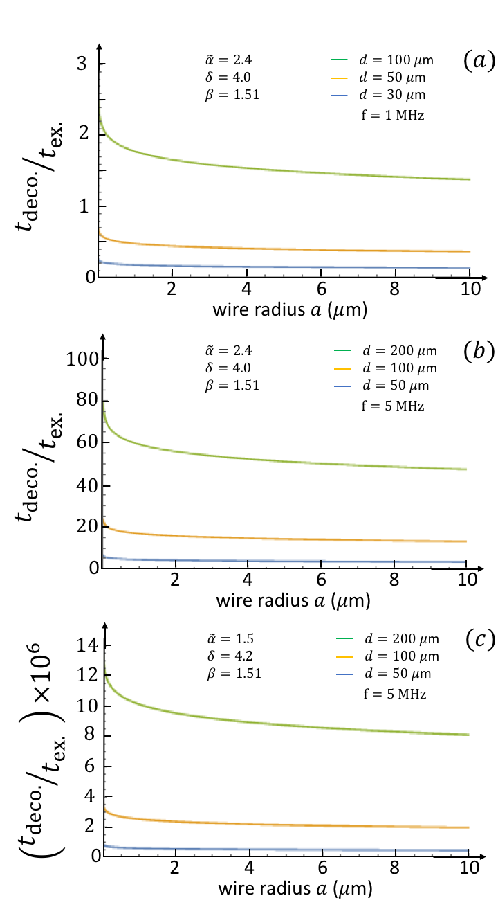
Figure 7: Ratio $t_{\mathrm{deco.}}/t_{\mathrm{ex.}}$ as a function of wire radius, for various parameter values. ($a$) shows a plot of $t_{\mathrm{deco.}}/t_{\mathrm{ex.}}$ as a function of the coupling wire’s radius $a$ for a set of parameter values for which equation (60) should be valid, based on experimental observations in Sedlacek et al. (2018a, b). Even for the best combination, $d=100~{}\mu$m and $f=1~{}$MHz, the criterion $t_{\mathrm{deco.}}/t_{\mathrm{ex.}}>10$ is not satisfied. ($b$) shows a similar plot made by assuming equation (60) continues to be valid up to $d=200~{}\mu$m and $f=5~{}$MHz (extrapolating). For these values, the criterion $t_{\mathrm{deco.}}/t_{\mathrm{ex.}}>10$ is satisfied. ($c$) shows that changes in the exponents $\tilde{\alpha}$ and $\delta$ can have a dramatic effect on the ratio $t_{\mathrm{deco.}}/t_{\mathrm{ex.}}$. This is illustrated using the least favorable values of $\tilde{\alpha}$ and $\delta$ listed in table 13. All panels are plotted for $\tilde{A}=0.012$ (or $A=1.8\times 10^{-22}$), $T=10~{}$K, $T_{\mathrm{p}}=10~{}$K and a wire length $l_{\mathrm{w}}=0.01~{}$m.

The dependence on $a$ is weak within the given range. Additionally, for all radii $a$ the ratio $t_{\mathrm{deco.}}/t_{\mathrm{ex.}}$ is less than $10$.

To achieve $t_{\mathrm{deco.}}/t_{\mathrm{ex.}}>10$ for $\tilde{\alpha}=2.4$, $\beta=1.51$, and $\delta=4.0$, we are obligated to let the frequency $f$ and distance $d$ exceed the known range of validity of equation (60). We assume the scaling for $d\bar{n}/dt$ as a function of $f$ and $d$ remains the same, and extrapolate equation (60) to higher frequencies and larger distances. Figure 7($b$) gives a sense of how far $f$ and $d$ must exceed known limits to reach $t_{\mathrm{deco.}}/t_{\mathrm{ex.}}>10$ by plotting equation (60) as a function of $a$ for $f=5~{}$MHz and $d=50~{}\mu$m, $d=100~{}\mu$m, $d=200~{}\mu$m. The upper two lines in figure 7($b$) suggest that for $\tilde{\alpha}=2.4$, $\beta=1.51$, and $\delta=4.0$, at $T=10~{}$K, and for an ion trapped $100~{}\mu$m or $200~{}\mu$m above a Nb surface, criterion i) is satisfied. This result is extremely sensitive to changes in $\tilde{\alpha}$ and $\delta$. We can look at what happens for the least favorable reported values of $\tilde{\alpha}$ and $\delta$ in table 13. The least favorable value of $\tilde{\alpha}$ is $\tilde{\alpha}=1.5$ (including the experimental uncertainty of $0.1$). The least favorable value of $\delta$ is $\delta=4.2$. With these, plotting equation (60) as a function of $a$ for $f=5~{}$MHz and $d=50~{}\mu$m, $100~{}\mu$m, $200~{}\mu$m gives a ratio $t_{\mathrm{deco.}}/t_{\mathrm{ex.}}$ on the order of $1\times 10^{-5}$ (figure 7($c$)). Achieving $t_{\mathrm{deco.}}/t_{\mathrm{ex.}}\sim 1$ for the combination $\tilde{\alpha}=1.5$, $\delta=4.2$, $\beta=1.51$ requires both high frequencies and large distances, for instance the combination $f=1~{}$GHz and $d=10~{}$cm. Such values are not feasible due to experimental limitations and make it unrealistic to satisfy criterion ii). Therefore, before undertaking an experiment to couple ions in separate traps it is important to characterize the ion trap and verify that $\tilde{\alpha}$ is large enough and $\delta$ is small enough to guarantee $t_{\mathrm{deco.}}/t_{\mathrm{ex.}}\geq 10$ for the targeted frequency and distance ranges.

Assuming the combination $\tilde{\alpha}=2.4$, $\delta=4.0$, and $\beta=1.51$ from Sedlacek et al. (2018a, b), we now plot equation (60) as a function of both $f$ and $d$. The three-dimensional surface plot in figure 8($a$) shows combinations of $f$ and $d$ for which $2\times t_{\mathrm{deco.}}/t_{\mathrm{ex.}}\geq 20$. (Scaling $t_{\mathrm{deco.}}/t_{\mathrm{ex.}}$ by a factor of $2$ improves the visualization.) This can be compared with the three-dimensional surface plot of $V_{\mathrm{sig.}}/V_{\mathrm{J.N.}}$ in figure 8(b) over the same ranges of $f$ and $d$, with a wire resistance $R=0.01~{}\Omega$, a frequency bandwidth $\Delta f=500~{}$Hz, the mass $m_{\mathrm{Be}}$ of a beryllium atom and charge $q_{\mathrm{c}}=4~{}e$. (The charge and resistance values used are different from the ones in table II, to make it easier to see the shape of the plot.) Ideally, a given coordinate in the frequency-distance plane should yield a value on the vertical axis greater than $20$ in figure 8($a$) and greater than $10$ in figure 8(b). However, values of $f$ and $d$ which increase $t_{\mathrm{deco.}}/t_{\mathrm{ex.}}$ tend to decrease $V_{\mathrm{sig.}}/V_{\mathrm{J.N.}}$ and vice-versa. If figure 8($a$) and figure 8(b) are superimposed, a compromise between the two criteria is reached for combinations of $f$ and $d$ that lie between the largest values on each surface. To visualize the target ranges clearly, we impose the ratio $t_{\mathrm{deco.}}/t_{\mathrm{ex.}}=10$ which specifies a single contour line in the $f-d$ plane in figure 8($a$). We also set $V_{\mathrm{sig.}}/V_{\mathrm{J.N.}}=10$ which specifies a contour line in figure 8(b). The two contour lines can be placed on a common set of coordinates, and if they overlap, the region between them yields values of $f$ and $d$ for which both the ratios $t_{\mathrm{deco.}}/t_{\mathrm{ex.}}$ and $V_{\mathrm{sig.}}/V_{\mathrm{J.N.}}$ are greater than $10$. Rearranging equations (60) and (63), the functions relating frequency $f$ to ion distance $d$ for the contour lines $t_{\mathrm{deco.}}/t_{\mathrm{ex.}}=10$ and $V_{\mathrm{sig.}}/V_{\mathrm{J.N.}}=10$ are:

$$f_{t_{\mathrm{deco.}}/t_{\mathrm{ex.}}}=\Bigg{(}10\times\left[\frac{2A\pi^{3}\epsilon_{\mathrm{o}}\times\left[1+\left(T/T_{\mathrm{p}}\right)^{\beta}\right]}{hd^{\delta+1}}\right]$$

$$\times\left[\left(\frac{2r+\frac{2\pi l}{8\mathrm{ln}\left(l/a\right)}}{r}\right)\left(\frac{\left(d^{2}+r^{2}\right)^{3}}{r^{2}}\right)\right]\Bigg{)}^{1/\left(\tilde{\alpha}-1\right)}~{},$$ (64)

and

$$f_{V_{\mathrm{sig.}}/V_{\mathrm{J.N.}}}=\frac{h}{8\pi^{2}m}\Bigg{(}\frac{1}{10}\times\left(\frac{1}{4k_{\mathrm{B}}T\Delta fR}\right)^{1/2}$$

$$\times\left(\frac{2}{2\times 8\epsilon_{\mathrm{o}}r+\frac{2\pi\epsilon_{\mathrm{o}}l}{\mathrm{ln}\left(l/a\right)}}\right)\times\frac{2q_{\mathrm{c}}r^{2}}{(r^{2}+d^{2}_{\mathrm{eq.}})^{3/2}}\Bigg{)}^{2}~{}.$$ (65)

Figure 8(c) shows a plot of equations (64) and (65) with common vertical and horizontal axes. The shaded region corresponds to combinations of $f$ and $d$ where the criteria $t_{\mathrm{deco.}}/t_{\mathrm{ex.}}=10$ and $V_{\mathrm{sig.}}/V_{\mathrm{J.N.}}=10$ are simultaneously satisfied.

The shaded region between the two curves increases rapidly with improved values of the exponents $\tilde{\alpha}$, $\delta$, and $\beta$. However, as it is not well understood how to control these exponents, the position of the curve for $t_{\mathrm{deco.}}/t_{\mathrm{ex.}}=10$ is fairly inflexible. (Decreasing the temperature below $T_{\mathrm{p}}\sim 10~{}$K provides little added benefit, and changing the wire radius is of limited use.) On the other hand, the contour line for $V_{\mathrm{sig.}}/V_{\mathrm{J.N.}}=10$ can be displaced in the $f-d$ plane by changing the temperature $T$ of the coupling system, the charge $q_{\mathrm{c}}$ or mass $m$ of the ion, the frequency range $\Delta f$ over which Johnson-Nyquist noise disturbs the system, or the resistance $R$ of the coupling wire. For instance, reducing the temperature from $T=10~{}$K to $T=0~{}$K causes the range of $f$ and $d$ for which both criteria are simultaneously satisfied to expand to infinity, as $V_{\mathrm{J.N.}}$ goes to zero. We observe that the right-most parentheses in equation (63), which depends on the mass $m$ and frequency of oscillation $f$ of the ion, is the spread (standard deviation of the position) of the zero-point wavefunction. This spread is $\sim 10~{}$nm for a ${}^{9}\mathrm{Be}^{+}$ ion oscillating at $5~{}$MHz. In section I.2.1 we chose this as the amplitude of oscillation of the ion, but the amplitude of oscillation can be increased by active driving. Ion shuttling experiments show that ions can be displaced without causing a loss of motional state coherence.

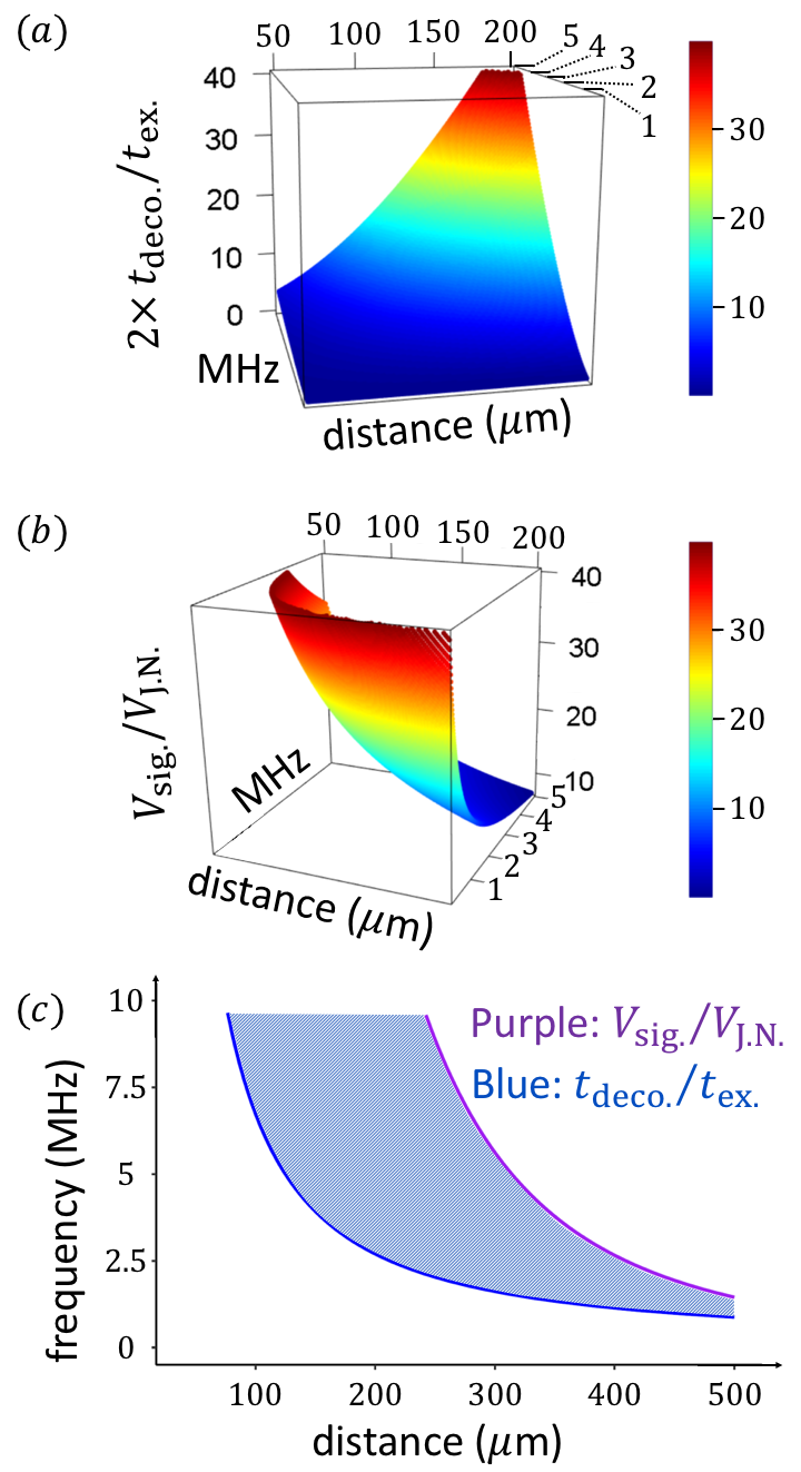
Figure 8: Simultaneously satisfying $t_{\mathrm{deco.}}/t_{\mathrm{ex.}}\geq 10$ and $V_{\mathrm{sig.}}/V_{\mathrm{J.N.}}\geq 10$. ($a$) A plot of $2\times t_{\mathrm{deco.}}/t_{\mathrm{ex.}}$ as a function of the distance $d$ between the ions and their respective pickup disks and the frequency $f$ at which the ions oscillate. Equation (60) is evaluated for the following parameters: $h$ is Plank’s constant, $\epsilon_{\mathrm{o}}$ is the vacuum permittivity, the heating coeff. $A=1.8\times 10^{-22}$, $T=10~{}$K, activation temperature $T_{\mathrm{p}}=10~{}$K, wire length $l_{\mathrm{w}}=0.01~{}$m, wire radius $a=10\times 10^{-6}~{}$m, disk radius $r=d/\sqrt{2}$, and the $1/f^{\tilde{\alpha}}$ heating exponents $\tilde{\alpha}=2.4$, $\delta=4.0$, and $\beta=1.51$ from Sedlacek et al. (2018a, b). ($b$) A plot of $V_{\mathrm{sig.}}/V_{\mathrm{J.N.}}$ for the same parameter values as in ($a$), with the following additions: $k_{\mathrm{B}}$ is Boltzmann’s constant, the coupling system temperature $T=10~{}$K, the motional mode frequency range $\Delta f=500~{}$Hz, wire resistance $R=0.01~{}\Omega$, charge $q_{\mathrm{c}}=4\times 1.6\times 10^{-19}~{}$C, and mass $m_{\mathrm{Be}}=1.5\times 10^{-26}~{}$kg. ($c$) Two contour lines: the blue contour corresponds to $t_{\mathrm{deco.}}/t_{\mathrm{ex.}}=10$ and the purple contour is for $V_{\mathrm{sig.}}/V_{\mathrm{J.N.}}=10$. Parameter values are the same as in ($a$) and ($b$) but with $R=0.0001~{}\Omega$ and charge $q_{\mathrm{c}}=e$.

Shuttling ions a distance of $280~{}\mu$m over the course of $5$ ion oscillations (in $3.6~{}\mu$s) has been achieved with motional heating below $0.1$ quantums Walther et al. (2012). This is equivalent to a displacement on the order of $50~{}\mu$m in one ion oscillation, suggesting that driving the ion could be exploited to increase the amplitude of oscillation to well over $1~{}\mu$m. This would increase $V_{\mathrm{sig.}}$ and hence the ratio $V_{\mathrm{sig.}}/V_{\mathrm{J.N.}}$ by a factor of $100$, allowing constraints on the Johnson-Nyquist noise to be relaxed by permitting a higher resistance $R$ of the coupling wire or a broader range of frequencies $\Delta f$ to interfere with the signal voltage.

An important step for future experiments is to measure $\tilde{\alpha}$, $\beta$, $\delta$, $A$, and $T_{\mathrm{p}}$ over the parameter ranges at which experiments are to be performed. This not only lays the foundation for using expression (60), but also confirms that expression (60) is valid for the targeted ranges of $f$, $T$, and $d$. For the example presently considered based on references Sedlacek et al. (2018a, b), and using figure 8(c), the target ranges of $f$, $d$, and $T$ are ($f=1~{}$MHz to $f=10~{}$MHz), ($d=50~{}\mu$m to $d=500~{}\mu$m), ($T=5~{}$K to $T=300~{}$K). A technical point for experiments is that the parameter ranges for $f$, $d$, and $T$ cannot be known before $\tilde{\alpha}$, $\beta$, $\delta$, $A$, and $T_{\mathrm{p}}$ are measured. This means $\tilde{\alpha}$, $\beta$, $\delta$, $A$, and $T_{\mathrm{p}}$ must initially be measured over arbitrarily chosen ranges of $f$, $d$, and $T$. Once initial values are determined, the ranges of $f$, $d$, and $T$ can be adjusted to ensure criteria i) and ii) are satisfied. It may be necessary to measure $\tilde{\alpha}$, $\beta$, $\delta$, $A$, and $T_{\mathrm{p}}$ a second time over the adjusted ranges of $f$, $d$, and $T$ to verify the validity of equation (60) for the adjusted ranges. Ultimately, before attempting the coupling experiment proposed herein, figure 8(c) should be replicated using experimentally measured values of $\tilde{\alpha}$, $\beta$, $\delta$, and $T_{\mathrm{p}}$ for the specific trap that will be used in experiments.

IV.4 Ranges of experimental parameters

The values of many parameters in equations (60) and (63) are bounded by experimental constraints. We now discuss these constraints, starting with the most rigid ones and progressing towards more flexible constraints.

The strongest constraints are the $1/f^{\tilde{\alpha}}$ (Anomalous noise) heating exponents $\delta$, $\tilde{\alpha}$, and $\beta$. These vary substantially between different trap setups and determine the scaling of the decoherence time with distance $d$, frequency $f$, and temperature $T$. The scaling exponents, along with the activation temperature $T_{\mathrm{p}}$, are presently difficult to control. Next, are the distance $d$, frequency $f$, and temperature $T$. For the experimentally measured coefficients $\tilde{\alpha}=2.4$, $\delta=4.0$, and $\beta=1.51$ in Sedlacek et al. (2018a, b), $d$, $f$, and $T$ are constrained by $1/f^{\tilde{\alpha}}$ noise to roughly $d>50~{}\mu$m, $f>2.5~{}$MHz, and $T<10~{}$K as shown by the blue curve for $t_{\mathrm{deco.}}/t_{\mathrm{ex.}}=10$ in figure 8(c) (plotted for $T=10~{}K$). With $d$ constrained by $1/f^{\tilde{\alpha}}$ heating, the radius of the pickup disk $r$ is also constrained, as we showed in section II.4 that the optimal relationship between $d$ and $r$ is $d_{\mathrm{eq.}}/\sqrt{2}\leq r_{\mathrm{opt.}}\leq d_{\mathrm{eq.}}$. Collectively, the above observations show that the main constraints for satisfying the criterion $t_{\mathrm{deco.}}/t_{\mathrm{ex.}}\geq 10$, described by equation (60), are imposed by $1/f^{\tilde{\alpha}}$ heating due to the trap electrodes.

Until now, we have used the notation $T$ to describe both the temperature of the trap electrodes, $T^{\mathrm{trap}}$ and the temperature of the coupling system, $T^{\mathrm{c.s.}}$. However, in practice these may be different. $T^{\mathrm{c.s.}}$ determines the impact of Johnson-Nyquist thermal noise and should be reduced as much as possible. For a superconducting coupling system, $T^{\mathrm{c.s.}}$ must be below the critical temperature $T_{\mathrm{c}}$ of the superconductor. The critical temperature of aluminum, which may be advantageous due to its long coherence length ($\xi\approx 1,600~{}$nm ), is $T^{\mathrm{Al}}_{\mathrm{c}}\sim 1~{}$K Hansen (2006). The critical temperature of niobium is $T^{\mathrm{Nb}}_{\mathrm{c}}\approx 9~{}$K.

The range of frequencies $\Delta f$ over which Johnson-Nyquist noise disturbs the system is determined by the range of frequencies transmitted via the coupling system. We want to transmit information encoded in motional modes of an ion, so $\Delta f$ is the range of frequencies that can excite these motional modes. Two factors influence this range. First, the intrinsic spread of frequencies which can induce a motional mode transition, known as the natural linewidth of the transition. Second, the jitter of the center frequency of the distribution as a whole due to technical noise. A motional mode transition can occur via a sideband transition of an ion, which involves a change in its internal state along with a change in its motional state. In the Lamb-Dicke regime, the spread of frequencies which induce a sideband transition is smaller than the spread of frequencies which induce a carrier transition (a change in internal state without an associated change in motional state). Thus, the natural linewidth of the carrier transition provides a bound on the natural linewidth of the sideband transition. Depending on the atomic species and atomic transition, this range can be quite narrow. To give an example, the natural linewidth of the carrier transition of the $6S_{1/2}$ to $5D_{3/2}$ electric-quadrupole transition in ¹³⁸Ba⁺ is $13~{}$mHz Kleczewski et al. (2012). This implies the natural linewidth of its sideband transition is less than $13~{}$mHz.

Technical noise influences the spacing between motional modes. The spacing between motional modes is given by $\hbar\omega$, the frequency of oscillation of the ion, which depends on the strength of the ion’s confinement in the trap. If the strength of confinement changes, for example due to fluctuations in the voltages on the trap electrodes, the spacing between motional modes also varies. This results in a shift of the center of the distribution of frequencies which excite the motional mode transition. If the center frequency shifts rapidly and by a large amount compared to the natural linewidth of the motional mode, the range of frequencies which induce motional mode transitions is effectively broadened. For changes in the motional modes that occur through sideband transitions, variations in the internal energy levels of the ion also contribute to jitter of the center frequency of the motional mode transition. However, this effect tends to be smaller than jitter due to variations in the trap potential. In practice, all factors which cause the motional mode energy levels to shift at high enough frequencies broaden the range of $\Delta f$. Reference Johnson et al. (2016) shows that technical noise on the sideband transition between two hyperfine states of the ¹⁷¹Yb⁺ ion can be reduced to $\Delta f\sim 500~{}$Hz. A further discussion of $\Delta f$ may be found in appendix J.

Next, we consider the wire resistance $R$. Figure 8(c) is plotted for a temperature $T=10~{}$K, and a wire of radius $a=10\times 10^{-6}~{}$m, length $l=1~{}$cm, and resistance $R=0.0001~{}\Omega$. A resistance of $R=0.0001~{}\Omega$ is difficult to achieve for a normal (non superconducting) wire of these dimensions. In appendix E, we use the expression $R\approx l_{\mathrm{w}}/\left(\sigma\pi a^{2}\right)$, where $\sigma$ is the electrical conductivity, and calculate a resistance $R\sim 0.003~{}\Omega$ for a cylindrical copper conducting wire with the dimensions above, with a conductivity $\sigma_{10\mathrm{K}}$ at $T=30~{}$K. Therefore, we recommend fabricating the coupling wire from a superconducting material to suppress Johnson-Nyquist noise and help satisfy the constraint $V_{\mathrm{sig.}}/V_{\mathrm{J.N.}}\geq 10~{}$. In figure 8(c), this equates to ensuring that the purple curve for $V_{\mathrm{sig.}}/V_{\mathrm{J.N.}}$ is positioned far enough to the right along the distance axis to allow the existence of the shaded overlap region. A more detailed discussion of resistance can be found in appendix E.

We now consider the wire radius $a$. Equations (60) and (63) for $t_{\mathrm{deco.}}/t_{\mathrm{ex.}}$ and $V_{\mathrm{sig.}}/V_{\mathrm{J.N.}}$ both depend on $a$ via the wire capacitance $C_{\mathrm{w}}=2\pi\epsilon_{\mathrm{o}}l_{\mathrm{w}}\big{/}\mathrm{ln}\left(l_{\mathrm{w}}/a\right)$. In the case of a normal conducting wire, $V_{\mathrm{sig.}}/V_{\mathrm{J.N.}}$ also depends on $a$ via the wire’s resistance $R=l_{\mathrm{w}}/\left(\sigma\pi a^{2}\right)$ (see equation (62) for an expression of $V_{\mathrm{sig.}}/V_{\mathrm{J.N.}}$ with $R$ explicitly written out). Increasing the cross-sectional area of a non superconducting cylindrical wire, in other words increasing its radius $a$, decreases the wire’s resistance and associated noise voltage. Overall, increasing $a$ decreases the ratio $t_{\mathrm{deco.}}/t_{\mathrm{ex.}}$, but for a normal conducting wire it increases $V_{\mathrm{sig.}}/V_{\mathrm{J.N.}}$. ($V_{\mathrm{sig.}}/V_{\mathrm{J.N.}}$ may also increase with $a$ for a superconducting wire, see appendix E). Since equations (60) and (63) both depend on the same parameter $a$ but respond to changes in $a$ in opposite ways, this leads to an optimization problem where, with all other parameters fixed, some values of $a$ may satisfy the criterion $t_{\mathrm{deco.}}/t_{\mathrm{ex.}}\geq 10$ but not $V_{\mathrm{sig.}}/V_{\mathrm{J.N.}}\geq 10$, or vice versa. Although figure 7 shows that the ratio $t_{\mathrm{deco.}}/t_{\mathrm{ex.}}$ only depends weakly on the wire radius $a$, optimization can be achieved by plotting both ratios as a function of $a$ and overlaying the two plots on the same graph with a common vertical axis (not shown here). This allows one to visualize which range of wire radiuses, if any, simultaneously satisfies $t_{\mathrm{ex.}}\geq 10$ and $V_{\mathrm{sig.}}/V_{\mathrm{J.N.}}\geq 10$, i.e. constraints i) and ii) in section IV.1. Given that $t_{\mathrm{deco.}}/t_{\mathrm{ex.}}$ only depends weakly on $a$, we assume it is generally preferable to improve $V_{\mathrm{sig.}}/V_{\mathrm{J.N.}}$ at the expense of $t_{\mathrm{deco.}}/t_{\mathrm{ex.}}$ by using larger wire radii and hence lower resistance.

In addition to the optimization outlined above, the choice of $a$ should take into account at least four other factors. First, for large wire radiuses, $a$ should remain small compared to the radii of the pickup disks, $a\ll r=d/\sqrt{2}$. This ensures the overall model of two pickup disks connected by a coupling wire remains valid. Second, the wire radius must respect $a\ll l_{\mathrm{w}}$ to avoid an unrealistic divergence of the expression $C_{\mathrm{w}}=2\pi\epsilon_{\mathrm{o}}l_{\mathrm{w}}\big{/}\mathrm{ln}\left(l_{\mathrm{w}}/a\right)$ for the capacitance of a thin wire (see for example figure 10 and the associated discussion in appendix K). Third, if one intends to use a superconducting wire, there is a minimum wire dimension at which superconductivity can be maintained, around $6~{}$nm according to Bezryadin et al. (2000), (see appendix E). This sets a minimum bound $5~{}\mathrm{nm}\lesssim a$. Fourth, for small wires the expression $R_{\mathrm{wire}}=l_{\mathrm{w}}/\left(\sigma\pi a^{2}\right)$ ceases to be valid. The limit of small wires requires a different expression for the resistance. The conductance $G$ becomes quantized and the resistance is given by a form of the Landauer formula, $1/R=G=\frac{e^{2}}{\pi\hbar}\sum_{n}T_{n}$ Landauer (1957), where $e$ is the charge of an electron, $\pi=3.14...$, $\hbar$ is the reduced Plank’s constant, the sum over $n$ is a sum over the number of conductive channels in the system, and $T_{n}$ are the transmission eigenvalues which describe the probability of transmission of an electron through the input interface and output interface of a conductor.

For the coupling system to be useful, the length $l_{\mathrm{w}}$ of the coupling wire should be long enough that the coupling system provides an advantage over direct free-space coupling via the Coulomb interaction. In other words, $\gamma$, which denotes the coupling strength via the conducting wire, should be larger than $\gamma_{\mathrm{Coul.}}$, which denotes the coupling strength via the direct Coulomb interaction. We can set the target $\gamma/\gamma_{\mathrm{Coul.}}\geq 10~{}$. For proof of concept purposes, it would also be nice to demonstrate a situation where the Coulomb interaction is not strong enough to achieve state exchange within the decoherence time of the ion, $t_{\mathrm{deco.}}/t^{\mathrm{Coul.}}_{\mathrm{ex.}}\leq 1$, but interaction via the coupling system is strong enough to achieve state exchange within the ion’s decoherence time, $t_{\mathrm{deco.}}/t_{\mathrm{ex.}}\geq 1$. This would prove that any observed state exchange happens via the wire. To design such a system, one must know the maximum distance $l_{\mathrm{Coul.}}$ at which state exchange via the Coulomb interaction can occur faster than the decoherence time. An inequality placing an upper bound on $l_{\mathrm{Coul.}}$ is derived in appendix K, expression (98). For intuition, we consider two singly-charged ${}^{9}\mathrm{Be}^{+}$ ions with mass $m=1.5\times 10^{-26}~{}$kg , trapped with an axial mode frequency $f=5~{}$MHz , and displaying a decoherence time $t_{\mathrm{deco.}}=0.32~{}$ seconds. In this system, the maximum distance $l_{\mathrm{Coul.}}$ at which state exchange can occur via direct Coulomb interaction is $l_{\mathrm{Coul.}}=0.5~{}$mm. Therefore, if a coupling system is designed with $l_{\mathrm{wire}}>0.5~{}$mm  and motional state exchange is observed, one can safely conclude the state exchange is occurring via the coupling system. We have used the length $l_{\mathrm{wire}}=1~{}$cm for illustrative calculations throughout this study. As shown in figure 10, appendix K, with this length the criterion $\gamma/\gamma_{\mathrm{Coul.}}\geq 10~{}$ is satisfied. However, to enhance the coupling strength and mitigate decoherence in the wire, for a proof-of-concept experiment we propose using a wire $l_{\mathrm{wire}}=1~{}$mm long, even though this length does not satisfy the target $\gamma/\gamma_{\mathrm{Coul.}}\geq 10~{}$.

Finally, the mass $m$ and charge $q_{\mathrm{c}}$ of the ion are somewhat flexible constraints. Indeed, equation (60) is independent of both these parameters. Equation (63) increases with smaller $m$ and larger $q_{\mathrm{c}}$. To maximize $V_{\mathrm{sig.}}/V_{\mathrm{J.N.}}$ it is advantageous to use particles with the lowest mass and the highest charge possible. As it is generally simplest to produce singly-charged ions, here we mainly consider $q_{\mathrm{c}}=1$ and the mass $m_{\mathrm{Be}}$ of a beryllium ion. However, by removing additional electrons the charge of a trapped ion may be increased up to around $q_{\mathrm{c}}=10$ Safronova et al. (2014). To reduce the mass as much as possible, a single electron qubit could also be considered, with a mass of $m_{\mathrm{e}}=9\times 10^{-31}~{}$kg $\approx\left(1/10,000\right)\times m_{\mathrm{Be}}$. For such a small mass it is important to verify the validity of the rotating wave approximation before applying the results for the exchange time $t_{\mathrm{ex.}}$ used in this work. The rotating wave approximation holds when the coupling between two harmonic oscillators is weaker than strength of the harmonic confinement, meaning in the limit $(\gamma/(m\omega^{2}))<0.1~{}$ Estes et al. (1968). For the value of $\gamma$ in table 2 for $d=50\times 10^{-6}~{}$m, $l_{\mathrm{w}}=0.01~{}$, and using the mass of an electron $m_{\mathrm{e}}=9.1\times 10^{-31}~{}$kg and a frequency $f=5~{}$ MHz, we find $(\gamma/(m\omega^{2}))\approx 0.02$ which is not far from the cutoff of $0.1$. However, trapped electrons typically oscillate at frequencies on the order of $f=100$ MHz. In this case, $(\gamma/(m\omega^{2}))\approx 4\times 10^{-5}\ll 0.1$ and the rotating wave approximation is verified. Although the prospect of using electrons is appealing, designing an experiment with electrons may require special considerations. Electrons are typically trapped in Penning traps rather than Paul traps, and other additional factors may need to be considered.

Table 6 provides a summary of the constraints discussed above along with their degree of flexibility. The values should be used as intuitive guidelines, but the given boundaries do not guarantee a frequency-distance diagram where both criteria $t_{\mathrm{deco.}}/t_{\mathrm{ex.}}>10$ and $V_{\mathrm{sig.}}/V_{\mathrm{J.N.}}>10$ are simultaneously satisfied, as in figure 8(c). In outlining the constraints, where relevant we assume the exponents $\tilde{\alpha}=2.4$, $\beta=1.51$, and $\delta=4.0$ for the parameters $f$, $d$, and $T$ respectively, which are a consistent combination for a Niobium trap, based on references Sedlacek et al. (2018a, b). Prior to implementing an experiment, the exponents $\tilde{\alpha}$, $\beta$, and $\delta$ should be measured for a specific target experimental system, and the diagram in figure 8(c) should be reproduced for a specified combination of parameters to check for a successful overlap region. For each parameter in table 6, a single inequality indicates the direction which increases both the ratios $t_{\mathrm{deco.}}/t_{\mathrm{ex.}}$ and $V_{\mathrm{sig.}}/V_{\mathrm{J.N.}}$. For cases where a given parameter increases one of the ratios but decreases the other, a general range is given. The Tunability columns give a sense of how much the ratio can be improved by tuning the indicated variable. Low tunability means if the variable is pushed to known experimental limits, roughly outlined in the Present limitation column, the ratio can be improved by a factor $\leq 5$. Moderate means $>5$ but $\leq 10$.

Table 6: Summary of variables and their suggested values and tunability. The Suggested value column gives a list of bounds based on experimental feasibility. If all of the bounds in this column are used to evaluate either $t_{\mathrm{deco.}}/t_{\mathrm{ex.}}$ or $V_{\mathrm{sig.}}/V_{\mathrm{J.N.}}$, they yield a result on the order of $10$. When two colored values are shown, the purple bound (top value) is chosen such that the ratio $t_{\mathrm{deco.}}/t_{\mathrm{ex.}}\approx 10$ , and the red bound (bottom value) is chosen such that the ratio $V_{\mathrm{sig.}}/V_{\mathrm{J.N.}}\approx 10$. Bounds given in black represent that, where applicable, the same value is used to evaluate $t_{\mathrm{deco.}}/t_{\mathrm{ex.}}$ and $V_{\mathrm{sig.}}/V_{\mathrm{J.N.}}$. For the wire radius, the value $a=10~{}\mu\mathrm{m}$ is used in all cases. The ratio $t_{\mathrm{deco.}}/t_{\mathrm{ex.}}$ is associated with $5$ free parameters, while $V_{\mathrm{sig.}}/V_{\mathrm{J.N.}}$ is associated with $9$ free parameters. Two of the free parameters associated with $V_{\mathrm{sig.}}/V_{\mathrm{J.N.}}$ have moderate tunability. This indicates that the ratio of coherence time to exchange time is a less flexible criterion than the signal to noise ratio for Johnson-Nyquist (thermal) noise.

Description	Variable	Suggested value	Tunability of $t_{\mathrm{deco.}}/t_{\mathrm{ex.}}$	Tunability of $V_{\mathrm{sig.}}/V_{\mathrm{J.N.}}$	Present limitation
Distance between ion and pickup disk	$d_{\mathrm{eq.}}$	${\color[rgb]{0.54,0.17,0.89}\geq 50~{}\mu\mathrm{m}}$, ${\color[rgb]{0.9,0.17,0.31}\leq 200~{}\mu\mathrm{m}}$	low	low	$\sim 50~{}\mu$m, ion heating from trap electrodes. a
Radius of pickup disk	$r$	$\approx d_{\mathrm{eq.}}/\sqrt{2}$	N.A.	N.A.	N.A.
Length of wire	$l_{\mathrm{w}}$	$\leq 1~{}$cm	low	low	$l_{\mathrm{w}}\sim 0.5~{}$mm. b
Motional mode range of frequencies  c	$\Delta f$	$\leq 500~{}$Hz	N.A.	low	$\leq 500~{}$Hz, due to stability of the trap Johnson et al. (2016).
Secular frequency	$f$	$\geq 5~{}\mathrm{MHz}$	low	low	$\sim 2.5$ MHz, heating of motional mode proportional to $1/f^{\tilde{\alpha}}$. a
Charge	$q_{\mathrm{c}}$	$\geq 1$	N.A.	moderate	Complexity of the experiment needed to ionize ions.
Mass  ${}^{d,~{}e}$	$m$	$\leq m_{{}_{{}^{9}\mathrm{Be}^{+}}}=1.5\times 10^{-26}~{}$kg	N.A.	low	No limit. Must be determined on case by case basis.
Wire radius	$a$	$100~{}\mathrm{nm}\leq a\leq 0.2\times d_{\mathrm{eq.}}/\sqrt{2}$	low	low, linked to $R$	$\sim 5~{}$nm, minimum radius at which superconductivity persists Bezryadin et al. (2000).
Temperature	$T$	$\leq 10$ degrees Kelvin	low	low	$\sim 5~{}$K , ion trap operation raises temperature above $4~{}$K  Chiaverini and Sage (2014).
Resistance  f	$R$	$\ll g\left(f,d_{\mathrm{eq.}},w\right)$ AND $\leq 0.001~{}\Omega$	N.A.	high	Minimal residual resistance of superconducting wire.

^a This effect is sometimes called Anomalous heating Leibfried et al. (2003); Deslauriers et al. (2006). See sections III.3, IV.2 and appendix I for further discussion.
^b At $f=5~{}$MHz , at $l_{\mathrm{w}}\sim 0.5~{}$mm the ratio $t_{\mathrm{deco.}}/t^{\mathrm{Coul.}}_{\mathrm{ex.}}\sim 1$ for two singly-charged ${}^{9}\mathrm{Be}^{+}$ ions coupled via direct Coulomb interaction (see appendix K). Therefore, at $l_{\mathrm{w}}\leq 0.5~{}$mm a coupling wire is theoretically not necessary.
^c The relevant range of frequencies $\Delta f$ is estimated in appendix J.
^d Suggested mass cutoff for the case $q_{\mathrm{c}}=1$, $R=0.001~{}\Omega$. If $q_{\mathrm{c}}>1$ or $R<0.001~{}\Omega$ the mass constraint can be relaxed and higher masses become more viable.
^e Electrons with mass $m_{\mathrm{e}}$ could also be explored, see section IV.4.
^f The function $g\left(f,d_{\mathrm{eq.}},w\right)$ is the resistance at which the ratio $V_{0}/V_{f}\sim 10$ after induced charge $Q_{\mathrm{transf.}}$ has drained off of a pickup disk, given the frequency of oscillation $f$ and assuming the pickup disk is grounded. See section I.3 for discussion. ^a This effect is sometimes also called Anomalous heating Leibfried et al. (2003); Deslauriers et al. (2006). See sections (LABEL:Flickernoise) and IV.2 for further discussion.
^b At $f=5~{}$MHz , at $l_{\mathrm{w}}\sim 0.5~{}$mm the ratio $t_{\mathrm{deco.}}/t^{\mathrm{Coul.}}_{\mathrm{ex.}}\sim 1$ for two singly-charged ${}^{9}\mathrm{Be}^{+}$ ions coupled via direct Coulomb interaction (see appendix K). Therefore, at $l_{\mathrm{w}}\leq 0.5~{}$mm a coupling wire is theoretically not necessary.
^c The relevant range of frequencies $\Delta f$ is estimated in appendix J.
^d Suggested mass cutoff for the case $q_{\mathrm{c}}=1$, $R=0.001~{}\Omega$. If $q_{\mathrm{c}}>1$ or $R<0.001~{}\Omega$ the mass constraint can be relaxed and higher masses become more viable.
^e Electrons with mass $m_{\mathrm{e}}$ could also be explored, see section IV.4.
^f The function $g\left(f,d_{\mathrm{eq.}},w\right)$ is the resistance at which the ratio $V_{0}/V_{f}\sim 10$ after induced charge $Q_{\mathrm{transf.}}$ has drained off of a pickup disk, given the frequency of oscillation $f$ and assuming the pickup disk is grounded. See section I.3 for discussion.

V A few considerations for implementing a practical system

In the previous section we considered experimental constraints on the parameters of the coupling system. Here, we discuss general considerations for a real implementation. We begin with the question of whether to use a single coupling wire, or two parallel coupling wires.

To minimize attenuation of the signal during propagation, one study Zurita-Sánchez and Henkel (2008) has proposed a design using two parallel coupling wires. For the present system such a transmission line design would not be helpful. At low frequencies, an electrical signal can propagate along a single conducting strand of wire with minimal losses. A rule of thumb is that a transmission line configuration is only necessary if the length of the wire $l_{\mathrm{w}}$ is greater than $1/4~{}$ of the propagating wavelength $\lambda$ Tra (a) (a cutoff of $1/10~{}$th of the propagating wavelength is also used Tra (b)). The trapped ions considered here oscillate with a frequency $f\sim 10~{}$MHz. For an electromagnetic wave in a conductor, the velocity factor $v/c$ is on the order of $0.5$, meaning the speed of propagation $v$ is $\sim~{}0.5~{}\times$ the speed of light. For a frequency $f\sim 10~{}$MHz, the wavelength is $\lambda=v/f\sim 15~{}$m. Since early experiments will likely attempt propagation over no more than a few centimeters, the approximation $\lambda\gg l_{\mathrm{w}}$ is valid.

The material from which the coupling wire is fabricated is also an important consideration. So far, we have used decoherence of the ions’ motional modes in the ions as the benchmark by which to gauge whether the exchange time $t_{\mathrm{ex.}}$ is short enough to successfully transfer quantum information between two ions. It is also important to consider whether and for how long quantum information can survive in the coupling system itself. In superconductors, the coherence length $\xi$ of Cooper pairs—the basic building blocks of superconductivity—can be over $1,600~{}$nm ($\xi\approx 1,600~{}$nm for Aluminium at $\sim 1~{}$K Hansen (2006)). A recent experiment successfully transferred quantum information over a distance of $\sim 3~{}$mm using a niobium superconducting wire cavity $600~{}$nm wide with a center frequency $f_{\mathrm{c}}=5.8~{}$GHz and quality factor $Q_{\mathrm{c}}=4,700$ Mi et al. (2018) (the coherence length for niobium is $\xi_{\mathrm{Nb}}=38~{}$nm). Additionally, a theoretical study spanning two publications predicts quantum information can propagate as an electric signal along a normal conducting lossy electrical transmission line Zurita-Sánchez and Henkel (2006, 2008). The work finds that a wire manifests properties of a string of harmonic oscillators, and shows that quantum information can be exchanged via a $1~{}$cm wire connecting two $100~{}\mu$m disks with a fidelity up to $0.989$ at a temperature of $4~{}$ Kelvin, for the coupling strengths in Zurita-Sánchez and Henkel (2008). The authors state: in the dispersive regime, conventional conductors, despite their intrinsic thermal resistive noise, do not necessarily degrade the coherent dynamics of the confined electrons on the timescale relevant for typical quantum manipulations. These results suggest that transferring quantum information using a conducting wire is feasible.

Several factors may hinder propagation of a quantum signal. Among these, dissipation can lead to decoherence Zurita-Sánchez and Henkel (2008). In a two-fluid model for superconductivity, a superconductor contains a superconducting component which carries current without interaction, along with a normal conducting component Weingarten (1996). The normal conducting electrons give rise to power dissipation from which a frequency-dependent surface resistance, or sheet resistance is defined as $R_{\mathrm{s}}=\frac{1}{2}\left(2\pi f\right)^{2}\mu^{2}_{0}\lambda_{\mathrm{L}}^{3}\sigma_{1}$, where $\mu_{0}$ is permeability, $\lambda_{\mathrm{L}}$ is the London penetration depth, and $\sigma_{1}$ is the normal state conductivity of the normal conducting electrons Hansen (2006); Weingarten (1996). This expression has been verified experimentally Hansen (2006). A precise description yields the BCS surface resistance, $R^{\mathrm{BCS}}_{\mathrm{s}}\propto f^{2}e^{-\Delta/k_{\mathrm{B}}T}/T$, where $f$ is frequency, $\Delta$ is defined to be half the Cooper pair binding energy, $k_{\mathrm{B}}$ is Boltzmann’s constant, $T$ is temperature in Kelvin, and $2\Delta\approx 3.5k_{\mathrm{B}}T_{\mathrm{c}}$, where $T_{\mathrm{c}}$ is the critical temperature of the superconductor Sup . For niobium with $T_{\mathrm{c}}=9.3~{}$K, at $T<T_{\mathrm{c}}/2$, $\Delta/k_{\mathrm{B}}\approx 17.67$ Sup . The BCS sheet resistance in ”Ohms per square” (not ”per square meter”), has been measured for niobium to be about $100~{}\mathrm{n}\Omega/\mathrm{square}$ at $T=4.2~{}$K and $1~{}$GHz, with extrapolation suggesting a decrease to about $1~{}\mathrm{n}\Omega~{}\mathrm{square}^{-1}$ at $10~{}$MHz Weingarten (1996). Other electrical noise may also exist in superconductors. In niobium at $4.2~{}$K, reference Weingarten (1996) measures a ”residual surface resistance” of $R_{\mathrm{res.}}\approx 1~{}\mathrm{n}\Omega~{}\mathrm{square}^{-1}$. This resistance is shown to be relatively frequency independent over the range of $\sim 100~{}$MHz to $100~{}$GHz Weingarten (1996). Additionally, in type II superconductors, there may be dissipative interactions involving the movement of weakly-pinned vortices Kogan (2008). Moreover, reference Boogaard et al. (2004) describes a spreading resistance associated with electrons flowing into or out of normal conducting reservoirs at either end of a superconducting wire. In some cases the spreading resistance is projected to be as large as $\sim~{}10~{}\mathrm{m}\Omega$ Boogaard et al. (2004). Radiation resistance could also lead to dissipation within the coupling system. Finally, in any realization, the pickup disks should connect to the coupling wire in a tapered fashion as indicated in figure 5, to ensure adiabatic flow of electrons between the disks and the coupling wire, reducing reflections and hence the possibility of shot noise Li et al. (1990). Appendix E discusses additional points related to resistance.

Photons emitted by the ion may destroy the superconductivity of the coupling system, leading to normal resistance and associated dissipation and decoherence. In a superconductor, superconductivity exists due to electrons in Cooper pairs which have zero resistance. If these Cooper pairs are broken, the electrons in the pair become ”normal electrons”. In BCS theory, if a material is in a superconducting state it is because the thermal energy $k_{\mathrm{B}}T$ is smaller than the binding energy of the Cooper pairs. Breaking Cooper pairs requires energy on the scale of the Cooper pair binding energy, $E_{\mathrm{C.p.}}=2\Delta\sim 1~{}$meV $=1.6\times 10^{-22}~{}$J Dressel (2013). The energy of a motional mode photon emitted by the ion is fixed by its motional frequency $f\sim 10\times 10^{6}~{}$Hz, and is $E^{\mathrm{motional}}_{\mathrm{ion}}=hf\sim 6.6\times 10^{-27}~{}$J where $h$ is Plank’s constant. Thus, motional photons from the trapped ions cannot break Cooper pairs. However, the frequency of optical photons emitted by the ions or used to address the internal orbital states of the ions is on the order of $E^{\mathrm{optical}}_{\mathrm{ion}}=100\times 10^{12}~{}$Hz. The extra seven orders of magnitude in energy means these are likely to break apart Cooper pairs. It could be necessary to take precautions to avoid exposing the superconducting coupling system to visible light or other high-energy photon sources.

For the layout of the device, the coupling system can be incorporated into a surface-trap configuration, which lends itself naturally to scaling. It can be manufactured using standard nanofabrication techniques, for example following the process we have outlined in Van Horne and Mukherjee (2020b), with additional steps to make the wire and introduce the coupling system within a planar trap. In the design outlined in Van Horne and Mukherjee (2020b), the pickup-disks are positioned on top of two pillars which stick out above the plane of the surface trap, to decrease the distance between the ions and the disks and thereby increase the coupling strength which scales strongly with distance, $\gamma\propto 1/d^{5}$. It should be noted that the configuration of pickup-disks protruding towards the trapped ions departs from the model used for the calculation of $\gamma_{\mathrm{pickup-disk}}$ in this work, since the pickup disks are no longer surrounded by an infinite ground plane. This results in fewer (zero) induced negative charges around the pickup-disk when a positively charged particle moves closer to it. Negative charges surrounding the pickup disk would exert a mutually repulsive force on negative charges in the disk, reducing the amount of negative charge that accumulates on the disk. Thus, without this effect the implementation in Van Horne and Mukherjee (2020b) presumably leads to a stronger coupling strength compared to the estimates in subsection II.5. If the majority of $1/f^{\tilde{\alpha}}$ (Anomalous) heating comes from effects happening in the plane of the trap electrodes or from the trap electrodes themselves, positioning the pickup disks close to the ions will not significantly increase $1/f^{\tilde{\alpha}}$ heating. With an equal heating rate and increased coupling strength, the ratio $t_{\mathrm{deco.}}/t_{\mathrm{ex.}}$ can be enhanced.

Since the signal-to-noise ratio for thermal noise scales with the charge of the trapped particles, $V_{\mathrm{sig.}}/V_{\mathrm{J.N.}}\propto q_{\mathrm{c}}$, using multiply-ionized species up to a maximum of about $q_{\mathrm{c}}=+10$ Safronova et al. (2014) can increase the ratio $V_{\mathrm{sig.}}/V_{\mathrm{J.N.}}$ by an order of magnitude. This strategy should not affect the ratio of coherence time to exchange time, $t_{\mathrm{deco.}}/t_{\mathrm{ex.}}$, which we have shown to be independent of the charge (equation (60)). It does, however, significantly reduce the coherence time $t_{\mathrm{deco.}}$ of the ion (equation (59)), as the $1/f^{\tilde{\alpha}}$ heating rate $d\bar{n}/dt$ scales with the charge squared (equation (58)).

VI Conclusions and outlook

This work suggests that despite the deleterious effects of $1/f^{\tilde{\alpha}}$ (Anomalous) heating, it is possible to exchange quantum information between ion qubits in separate surface traps using a conducting wire. Moreover, this can be achieved using existing technologies and materials, and singly-charged ions. However, successful implementation is subject to a number of engineering requirements.

Based on the observed variability of $1/f^{\tilde{\alpha}}$ noise in published literature, $1/f^{\tilde{\alpha}}$ noise is predicted to be one of the main constraints on the proposed scheme. As part of designing an experiment, it is strongly recommended to measure the exponents $\tilde{\alpha}$, $\delta$, and $\beta$ which characterize $1/f^{\tilde{\alpha}}$ noise in the setup, to ensure anomalous heating is low enough that quantum state exchange is theoretically possible, and $t_{\mathrm{deco.}}/t_{\mathrm{ex.}}\geq 10$. Working at cryogenic temperatures below $T=10~{}$K is also advised in early experiments, for two reasons. First, temperatures down to about $10~{}$K have been shown to suppress $1/f^{\tilde{\alpha}}$ noise, lengthening coherence time and hence increasing the ratio of coherence time to information exchange time, $t_{\mathrm{deco.}}/t_{\mathrm{ex.}}$. Second, low temperature favors superconductivity. The low resistance offered by a superconducting wire reduces thermal (Johnson-Nyquist) noise in the coupling wire, increasing the signal-to-noise ratio $V_{\mathrm{sig.}}/V_{\mathrm{J.N.}}$. Using a superconducting wire is also beneficial to reduce or eliminate shot (Shottky) noise.

Next, we recommend stabilizing ion traps to around $\Delta f\leq 500~{}$Hz to minimize the bandwidth over which the ions absorb noise. For the same reason, it could be desirable to turn off lasers during the transfer of motional quantum information, to avoid broadening the absorption spectrum $\Delta f$ of the motional mode transitions. Reducing $\Delta f$ reduces thermal or other noise which disturbs the system, and helps increase the signal-to-noise ratio.

Regarding the layout of the system, optimization of the design herein leads to a rule of thumb which relates the distance $d_{\mathrm{eq.}}$ between a trapped ion and a nearby pickup disk, to the optimal radius $r_{\mathrm{opt.}}$ of the disk. When the pickup disks’ capacitance is much larger than the capacitance of the connecting wire, the optimal relationship is $r_{\mathrm{opt.}}=d_{\mathrm{eq.}}$. When the wire capacitance is much larger than the disk capacitance, $r_{\mathrm{opt.}}=d_{\mathrm{eq.}}/\sqrt{2}$. In general, $d_{\mathrm{eq.}}/\sqrt{2}\leq r_{\mathrm{opt.}}\leq d_{\mathrm{eq.}}$.

Although the technology for interconnecting ion qubits using conducting wires already has the potential to be viable, over the long run there is room for progress which could lead to increased robustness and relaxed constraints. This can happen in several ways. First, if coupling designs such as the one outlined in Van Horne and Mukherjee (2020b) increase the coupling strength $\gamma$ without significantly increasing $1/f^{\tilde{\alpha}}$ heating noise, state exchange times $t_{\mathrm{ex.}}$ could be significantly reduced. Second, in the future $1/f^{\tilde{\alpha}}$ surface heating noise may become better understood and ways could be found to diminish it, thereby increasing coherence times $t_{\mathrm{deco.}}$. For instance, if $1/f^{\tilde{\alpha}}$ heating is activated by processes related to the $\sim$MHz rf trapping frequencies used in Paul traps, using Penning traps which do not require A.C. fields could be a way forwards. (Calculations suggest black-body radiation cannot account for the observed heating rates. The energy which causes $1/f^{\alpha}$ ion heating must come from somewhere, and it appears to be radiated from rf trap electrodes (see appendix I.1).) While some of the derivations herein may need to be revisited for Penning traps, their adaptation and applicability is likely straight forwards. Both of the advances above would allow transfer of quantum information at higher temperatures and over longer distances.

In this work we have focused on results which are immediately applicable for a planar coupling system, due to the potential for planar systems to be scaled. Other systems may be less suited to scalability but could facilitate exchange of quantum information. We hope the analysis and methodology developed herein will provide a foundation for a rich set of future studies and experiments. On this note, we wish the reader well in their scientific pursuits.

Appendix A Charge in an outer ring of a conducting disk; justification of the ’ring of charge’ approximation

We claim that when charges are placed on a conducting disk, most of the charges end up in a ”ring” around the edges of the disk. To justify this, one must demonstrate that at equilibrium, most of the charge is located in an annular segment of the disk with a width $\xi\ll$ than the radius of the disk. In this appendix the radius of the disk will be called ”$a$”, following the notation in McDonald (2003). We define ”$\xi\ll a$” to mean $\xi\leq\frac{a}{4}$, and ”most of the charge” to mean that at least $\frac{3}{4}\times Q$ should be within the annular segment covered by $\xi$, where $Q$ is the total charge on the disk. Following McDonald McDonald (2002), and Sir Thompson (Lord Kelvin) Thomson (Lord Kelvin), the surface charge density of a circular disk over most of its surface area (the parts near the edges of the disk notwithstanding), is given by $\sigma_{\mathrm{circular~{}disk}}(r)=\frac{Q^{\prime}}{4\pi a\sqrt{a^{2}-r^{2}}}$, where $a$ is the radius of the disk, $r$ is the distance away from the center of the disk at which the surface charge density is evaluated, and $Q^{\prime}$ is a parameter to be determined, (which would be the total charge $Q$ of the two flat surfaces combined, in the limit that the height $2b$ of the disk is $2b=0$). A more accurate description of the surface charge density near a corner is given by: $\sigma_{s}=\frac{K}{\sqrt[3]{s}}$, where $K$ is a constant and $s$ is distance away from the corner Jackson (1999) McDonald (2003). In the thin disk system, the intersection between the top (or bottom) face of the disk, and the side of the disk, produces a corner which extends as a ring around the center of the disk. The variable ”$s$” describes moving inwards a distance ”$s$” from the $90^{\mathrm{o}}$-corner edge of the ring, where $s\leq b$, and $2b$ is the height of the disk. The same expression $\sigma_{s}=\frac{K}{\sqrt[3]{s}}$ can be used to describe the charge density on the side of the disk, moving away from the $90^{\mathrm{o}}$-corners, towards the center of the rectangular strip which wraps around the circumference of the disk. To ensure consistency there must be continuity of charge density at every point on the top (and bottom) surface of the disk. Therefore, somewhere on the disk $\sigma_{\mathrm{circular~{}disk}}(r)=\sigma_{s}(s)$. We can postulate that this occurs a distance $b$ inwards from the edge of the disk, and then allow the free parameter $Q^{\prime}$ to vary in such a way as to satisfy the constraint that the total charge on the disk must sum up to $Q$. Continuity of charge density imposes: $K\big{/}\sqrt[3]{b}=Q^{\prime}\big{/}4\pi a\sqrt{a^{2}-(a-b)^{2}}$, or

$$K=\frac{Q^{\prime}b^{1/3}}{4\pi a\sqrt{a^{2}-(a-b)^{2}}}$$ (66)

The total charge contained in the region ”near the corners” of the disk can be found by integrating $\sigma_{s}$ a distance $b$ (in other words, half the disk-height) from the top-corner towards the center of the rectangular strip, from the bottom-corner towards the center of the rectangular strip, and also inwards forming an ’outer ring’ of charge on the top and bottom faces of the disk. This yields $Q_{s}=4\int_{0}^{b}\!\frac{K}{\sqrt[3]{s}}2\pi a\ ds=\frac{3b}{\sqrt{a^{2}-{(a-b)}^{2}}}Q^{\prime}$, where we have substituted expression (66) in for $K$. The total charge on the rest of the disk, over two ’inner small disks’ on the top and bottom faces, may be found by integrating $\sigma_{\mathrm{circular~{}disk}}$ from $r=0$ to $r=\left(a-b\right)$. This yields $Q_{g}=2\int_{0}^{a-b}\frac{Q^{\prime}}{4\pi a\sqrt{a^{2}-{r}^{2}}}2\pi rdr=\left(1-\frac{\sqrt{a^{2}-{(a-b)}^{2}}}{a}\right)Q^{\prime}$. The sum of these two expressions gives the total charge on the disk, $Q=Q_{g}+Q_{s}$, which provides a relationship between $Q$ and $Q^{\prime}$:

$$Q^{\prime}=\frac{Q}{\frac{3b}{\sqrt{a^{2}-{(a-b)}^{2}}}+1-\frac{\sqrt{a^{2}-{(a-b)}^{2}}}{a}}$$ (67)

In the limit $a\gg b$, expression (67) reduces to $Q^{\prime}\approx Q~{}$, which can be understood intuitively. When the disk is thin compared to its radius, only a small percent of its charge resides on the thin edge perpendicular to the circular faces of the disk.

We want to find the charge contained in the outer-ring region a distance $\xi\leq\frac{a}{4}$ away from the corner. In some cases, if the width $2b$ of the conducting disk is large compared to the radius $a$ of the disk, the distance $b$ inwards from the side of the disk may be greater than $\frac{a}{4}$. In this case, it makes sense to only use the expression for the charge density ”near a corner” to calculate the charge in the outer-ring $\xi\leq\frac{a}{4}$. Experimentally, the typical thickness of surface-trap electrodes ranges from $2b=100~{}$nm to $2b=10~{}\mu$m Labaziewicz et al. (2008); Hite et al. (2012); Daniilidis et al. (2014); Sedlacek et al. (2018a), and for what follows we consider a thickness up to $2b=35~{}\mu$m. From section II.4, for the limiting case where the disk capacitance is much greater than the wire capacitance, the optimal relationship between the radius of the disk and the equilibrium height of the suspended ion is $r\sim d_{\mathrm{eq.}}/\sqrt{2}$ (here, the notation ”$r$” refers to the standard notation used throughout the rest of the article, outside of this appendix). Throughout this article we have used the two example values $d=50~{}\mu$m and $d=200~{}\mu$m, which respectively imply disk radii of $a=\frac{1}{\sqrt{2}}50~{}\mu\mathrm{m}=35~{}\mu$m, and $a=\frac{1}{\sqrt{2}}200~{}\mu\mathrm{m}\sim 140~{}\mu$m. We can calculate the charge in the outer ring for the two extreme aspect ratios: ($2b=35~{}\mu$m, $a=35~{}\mu$m), and ($2b=100~{}$nm, $a=140~{}\mu$m).

In the first case, the thickness $\xi=a/4$ of the outer ring is equal to $b/2$. Since here $a/4$ is less than $b$, we only use the expression for the charge density ”near a corner” to calculate the charge in the outer-ring $\xi\leq\frac{a}{4}$. We must calculate the charge on the side of the disk, as well as inwards a distance $b/2$ towards the center of the disk. The charge on the side of the disk is $Q_{s}/2$. The charge inwards a distance $b/2$ towards the center of the disk, for the top and bottom faces is $2\int_{0}^{b/2}\!\frac{K}{\sqrt[3]{s}}2\pi a\ ds=\frac{3bQ^{\prime}}{2^{5/3}\sqrt{a^{2}-(a-b)^{2}}}$. Adding these together, the total charge in the region $\xi\leq\frac{a}{4}$ is

$$Q^{\xi\leq\frac{a}{4}}_{\mathrm{Edges}}=\frac{3b\left(2^{2/3}+1\right)}{2^{5/3}\sqrt{a^{2}-(a-b)^{2}}}Q^{\prime}$$ (68)

Plugging in the relationship between $Q^{\prime}$ and $Q$ from (67), and evaluating for $b=17.5~{}\mu$m, $a=35~{}\mu$m, yields $Q^{\xi\leq\frac{a}{4}}_{\mathrm{Edges}}\sim 0.76Q$. Hence, the approximation of a ring of charge is justified.

Next, we look at the second case, for a thinner disk. Now, $b=\xi=0.05~{}\mu$m is significantly less than $\frac{a}{4}=35~{}\mu$m, so the amount of charge contained in the thin sliver defined by $b$ is small compared to the total charge on the disk. To find the charge in the region $\xi\leq\frac{a}{4}=35~{}\mu$m we cannot only consider the ”edges” of the disk. Indeed, since $b/a$ is small and the ratio of charge in the region $s<b~{}$, to the charge in the rest of the disk, is small, one could consider using only the expression for the charge density on the circular surface $\sigma_{\mathrm{circular~{}disk}}(r)=\frac{Q^{\prime}}{4\pi a\sqrt{a^{2}-r^{2}}}$. In any case, this expression should be valid in the region $r<\frac{3}{4}a$. To avoid worrying about what happens near the edges of the disk, since $b<a/4$, we can use a short-cut and calculate the charge at a distance $\xi\geq\frac{a}{4}$ away from the edges, or in other words, the charge in the central part of the disk. We use the same integral as used to calculate $Q_{g}$ (above equation (67)), but integrate from $r=0$ to $r=\frac{3}{4}a$. Thus, $Q^{\mathrm{central}}=2\int_{0}^{3a/4}\frac{Q^{\prime}}{4\pi a\sqrt{a^{2}-{r}^{2}}}2\pi rdr=\left(1-\sqrt{\frac{7}{16}}\right)Q^{\prime}$. Plugging in the relationship between $Q^{\prime}$ and $Q$ from (67), and evaluating for $b=50~{}$nm, $a=140~{}\mu$m, yields $Q^{\mathrm{central}}=0.33Q$. The charge in the outer annular region, $Q^{\xi\leq\frac{a}{4}}_{\mathrm{Edges}}~{}$, is $Q$ minus the charge in the central area, in other words $Q^{\xi\leq\frac{a}{4}}_{\mathrm{Edges}}=Q-0.33Q=0.67Q$. In this case our criterion for ”most of the charge” ($75\%$) being in the annular segment covered by $\xi\leq\frac{a}{4}$ is not satisfied, but it is not too far off. If we calculate $Q^{\mathrm{central}}$ for the region from $r=0$ to $r=a/2$, we find $Q^{\mathrm{central}}=\left(1-\sqrt{3/4}\right)Q^{\prime}=0.13~{}Q^{\prime}$ $\approx 0.13~{}Q~{}$, which means over $86\%$ of the charge is contained in the region $r\geq a/2$. Thus, although the approximation that charge distributes in a ’ring’ becomes less accurate for thinner disks, the approximation is still reasonably well justified.

The analysis above can be supplemented with an additional observation. We showed that more than $50~{}\%$ of the charge lies in the $r\geq a/2$ region, but this region also accounts for more than $50~{}\%$ of the surface-area of the disk. Our calculations do not inform us about the charge density throughout the disk. For this we recall the expression for the charge density, which in the limit of a thin disk ($Q^{\prime}\approx Q~{}$) is $\sigma_{\mathrm{circular~{}disk}}(r)=\frac{Q}{4\pi a\sqrt{a^{2}-r^{2}}}~{}$ McDonald (2002); Thomson (Lord Kelvin) . This expression depends on the radial distance $r$ from the center of the disk, and increases continuously as $r$ approaches $a$. It guarantees the charge density is not, for instance, homogeneous across the disk. Although we do not know a priori whether representing the surface-charge distribution on a conducting disk as a ring is more accurate than representing it as a homogeneous distribution, we can say by looking at the charge density that the ring of charge model is both plausible and consistent with known results.

To put numbers to the theoretical results above, we calculate an average charge density for the two regions, ($r=3a/4$ to $r=a$), and ($r=a/2$ to $r=a$), using the expression for a thin disk. The area of the first region is $\pi a^{2}-\pi\left(\frac{3}{4}a\right)^{2}=\pi a^{2}\left(\frac{7}{16}\right)$. The charge density in this region is then $\rho^{\xi\leq\frac{a}{4}}=\frac{16}{7}\times 0.67~{}Q/\left(\pi a^{2}\right)$. The area of the second region is $\pi a^{2}\left(\frac{12}{16}\right)$. The charge density in this region is $\rho^{\xi\leq\frac{a}{2}}=\frac{16}{12}\times 0.86~{}Q/\left(\pi a^{2}\right)$. Since $\frac{16}{7}\times 0.67=1.53$, while $\frac{16}{12}\times 0.86=1.15$, the charge density nearer to the edge of the disk is greater than the charge density closer to the center of the disk.

Appendix B The distribution of charge on connected conducting self-capacitors

B.1 Two connected metallic self-capacitors

To help guide intuition, a system of two capacitors connected by a wire with zero capacitance can be mapped to a system of two springs anchored to two walls on either side, and joined together in the middle. We imagine that the springs are initially disconnected from one another, and then pulled together, attached, and left to equilibrate. Therefore, at equilibrium both springs are somewhat stretched. The conversion of quantities from a system of springs to a system of electrical components is as follows:

$$\vec{F}=\pm k\Delta\vec{x}\qquad\longleftrightarrow\qquad\vec{V}=\pm\left(\frac{1}{C}\right)\vec{Q}$$ (69)

Specifically, $\vec{F}\leftrightarrow\vec{V}$, $k\leftrightarrow\frac{1}{C}$, and $\Delta\vec{x}\leftrightarrow\vec{Q}$. Here, $\vec{V}\mathrm{and}~{}\vec{Q}$ are described as vectors to denote that they can be positive or negative along a one-dimensional number line. The $\pm$ denotes that the direction of the force depends on which side of the spring one displaces, while keeping in mind that $\Delta\vec{x}$ is always measured as a positive number (see figure 9). The leftward force due to the leftmost spring is $\vec{F}_{a}=-(k_{a}\Delta\vec{x}_{a})$, while the right-ward force due to the rightmost spring is $\vec{F}_{c}=k_{c}\Delta\vec{x}_{c}$, where $\Delta\vec{x}_{a}$ and $\Delta\vec{x}_{c}$ are both positive numbers measured along the same $x$-axis. At equilibrium the leftward force and the rightward force must have the same magnitude and opposite direction, so: $\vec{F_{a}}=-\vec{F_{c}}$. Hence, $k_{a}\Delta\vec{x_{a}}=k_{c}\Delta\vec{x_{c}}$, which translates to $\frac{1}{C_{a}}\vec{Q}_{a}=\frac{1}{C_{c}}\vec{Q}_{c}$. Thus, $C_{a}=C_{c}$ implies $\vec{Q}_{a}=\vec{Q}_{c}$.

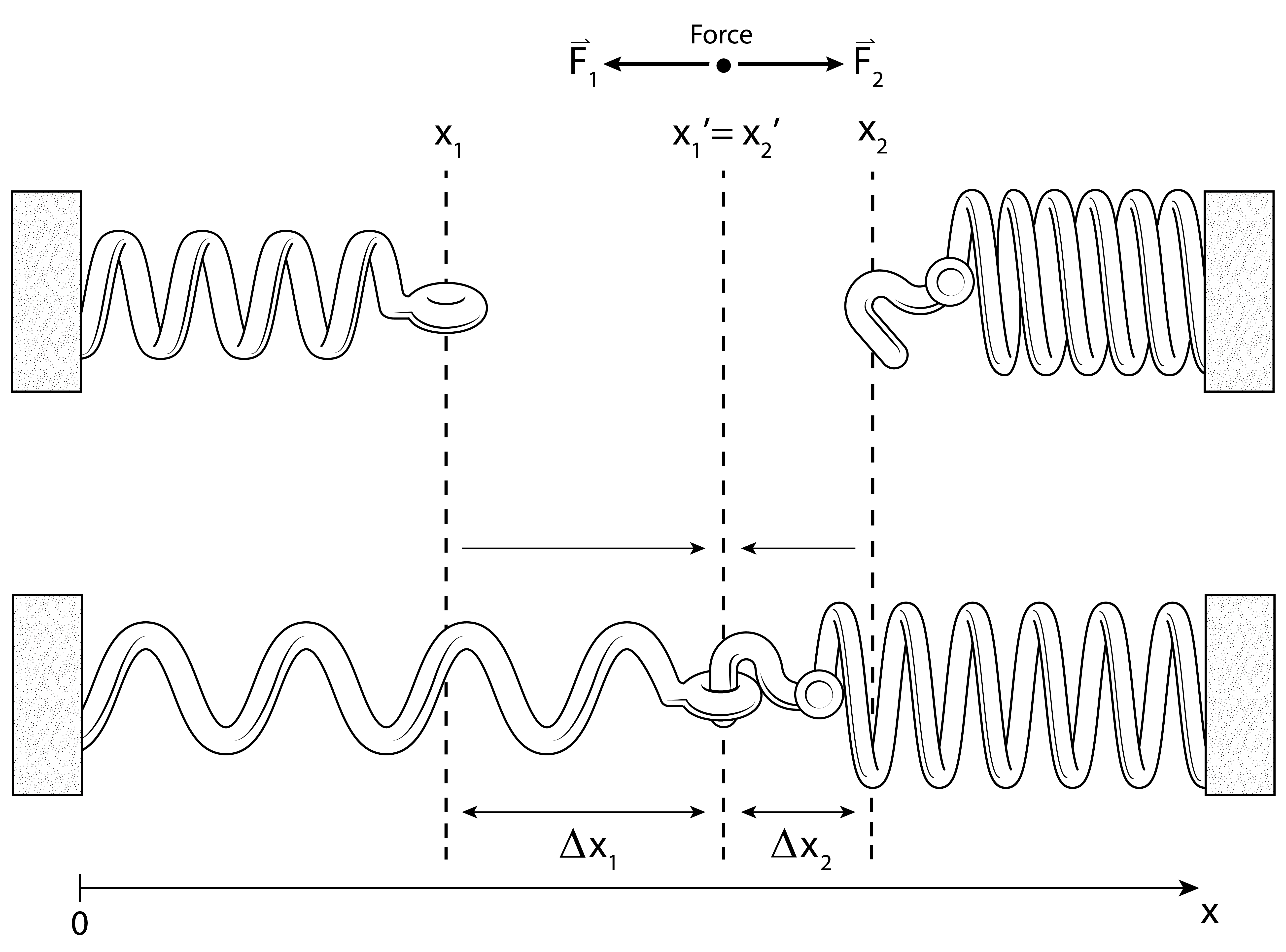
Figure 9: Two connected springs. (Top) Two springs attached to walls are disconnected and in a relaxed position. (Bottom) The two springs are brought together, attached, and then allowed to relax to the equilibrium state shown. The notations $\vec{F_{1}}$ and $\Delta\vec{x}_{1}$ in the figure correspond to $\vec{F_{a}}$ and $\Delta\vec{x}_{a}$ in the text, and similarly for $\vec{F_{2}}$.

B.2 Three connected metallic self-capacitors

The same reasoning is followed as in section B.1, but now with an additional third spring placed between spring $a$ and spring $c$, called spring $b$. This leads to the following two equations:

$$k_{a}\Delta\vec{x_{a}}=k_{\mathrm{eq_{1}}}\left(\Delta\vec{x_{b}}+\Delta\vec{x_{c}}\right)$$ (70)

$$k_{c}\Delta\vec{x_{c}}=k_{\mathrm{eq_{2}}}\left(\Delta\vec{x_{a}}+\Delta\vec{x_{b}}\right)$$ (71)

The notation $k_{\mathrm{eq_{1}}}$ refers to the equivalent spring constant of the two springs $k_{b}$ and $k_{c}$ in series, and $\left(\Delta\vec{x_{b}}+\Delta\vec{x_{c}}\right)$ is the total distance by which this equivalent spring is stretched. Solving (71) for $\Delta\vec{x_{b}}$ gives $\Delta\vec{x_{b}}=\frac{k_{c}\Delta\vec{x_{c}}}{k_{\mathrm{eq2}}}-\Delta\vec{x_{a}}$, which can be inserted into equation (70). Re-arranging (70) then leads to:

$$\Delta\vec{x_{c}}=\Delta\vec{x_{a}}\left(1+\frac{k_{a}}{k_{\mathrm{eq1}}}\right)\left(\frac{1}{\frac{k_{c}}{k_{\mathrm{eq2}}}+1}\right)~{}.$$ (72)

Writing out $k_{\mathrm{eq1}}=\frac{k_{b}k_{c}}{k_{b}+k_{c}}$, $k_{\mathrm{eq2}}=\frac{k_{a}k_{b}}{k_{a}+k_{b}}$ and substituting $\frac{1}{C_{i}}$ with $i=a,b,c$ for $k_{i}$, and $Q_{i}$ for $\Delta\vec{x_{i}}$ gives (after simplification):

$$Q_{c}=Q_{a}\left(1+\frac{C_{c}+C_{b}}{C_{a}}\right)\left(\frac{1}{1+\frac{C_{b}+C_{a}}{C_{c}}}\right)$$ (73)

which further reduces to $Q_{c}=Q_{a}\frac{C_{c}}{C_{a}}$. If $C_{a}=C_{c}$, then $Q_{a}=Q_{c}$, the same as was concluded in section B.1. Similarly, a relationship can be derived between $\Delta\vec{x_{c}}$ and $\Delta\vec{x_{b}}$,

$$\Delta\vec{x_{c}}=\Delta\vec{x_{b}}\left(1+\frac{k_{a}}{k_{\mathrm{eq1}}}\right)\left(\frac{1}{\left(\frac{k_{a}}{k_{\mathrm{eq1}}}\right)\frac{k_{c}}{k_{\mathrm{eq2}}}-1}\right)~{}.$$ (74)

This leads to the relationship between $Q_{c}$ and $Q_{b}$:

$$Q_{c}=~{} Q_{b}\left(1+\frac{C_{c}+C_{b}}{C_{a}}\right)$$ (75)

$$~{}~{}~{}~{}~{}~{}\times~{}\left(\frac{1}{\left(1+\frac{C_{b}}{C_{c}})\right)\left(1+\frac{C_{b}}{C_{a}}\right)-1}\right)~{},$$

which further reduces to $Q_{c}=Q_{b}\frac{C_{c}}{C_{b}}$.

B.3 Expressing the charge $Q_{c}$ in terms of $Q_{\mathrm{transf.}}$

Section B.2 provides expressions for $Q_{c}$ in terms of $Q_{a}$, and for $Q_{c}$ in terms of $Q_{b}$. However, the final intent is to find the charge deficit (or surplus) that results on disk2, when ion#1 moves closer (or farther away from) disk1. What is known is the amount of charge $Q_{\mathrm{transf.}}$ which would flow onto disk1, if it were connected to ground. This provides the total energy brought to disk1 by the movement of ion#1,  $E=\frac{Q^{2}_{\mathrm{transf.}}}{2\left(C_{a}+C_{b}+C_{c}\right)}$,  where $C_{a}=C_{\mathrm{disk1}}$, $C_{b}=C_{\mathrm{wire}}$, and $C_{c}=C_{\mathrm{disk2}}$. What remains unknown is how this energy will distribute among $C_{a}$, $C_{b}$, and $C_{c}$, when the system adjusts to the new potential. (Presumably this adjustment occurs adiabatically, since the resistance $R_{\mathrm{wire}}$ and inductance $L_{\mathrm{wire}}$ is low enough for the charge to flow between the capacitors much more quickly than the period of one oscillation. See subsection I.3, and appendices E and H). Specifically, the aim is to determine the amount of charge which ends up on $C_{c}$, which determines the strength of the resulting force on ion#2 when ion#1 moves. From the results of section B.2, it is now possible to express $Q_{c}$ in terms of $Q_{\mathrm{transf.}}$. With $C_{\mathrm{tot.}}\equiv\left(C_{a}+C_{b}+C_{c}\right)~{}$,

$$E=\frac{Q^{2}_{\mathrm{transf.}}}{2C_{\mathrm{tot.}}}=\frac{Q^{2}_{a}}{2C_{a}}+\frac{Q^{2}_{b}}{2C_{b}}+\frac{Q^{2}_{c}}{2C_{c}}~{}.$$ (76)

Using (73) and (75),  and the notation $\Lambda$ and $\Upsilon$ for the portions which depend on capacitance in (73) and (75), respectively (so that, e.g. $Q_{c}=Q_{a}\Lambda$) this becomes

$$\frac{Q^{2}_{\mathrm{transf.}}}{2C_{\mathrm{tot.}}}=\frac{Q^{2}_{c}}{2}\left(\frac{1}{C_{a}\left(\Lambda^{2}\right)}+\frac{1}{C_{b}\left(\Upsilon^{2}\right)}+\frac{1}{C_{c}}\right)~{},$$

which re-arranges to

$$Q_{c}=\frac{1}{\sqrt{\left(\frac{1}{C_{a}\left(\Lambda^{2}\right)}+\frac{1}{C_{b}\left(\Upsilon^{2}\right)}+\frac{1}{C_{c}}\right)C_{\mathrm{tot.}}}}Q_{\mathrm{transf.}}~{},$$ (77)

and further simplifies to:
$Q_{c}=\left(C_{c}~{}/~{}\left(C_{a}+C_{b}+C_{c}\right)\right)Q_{\mathrm{transf.}}$. This can be summarized succinctly as $Q_{c}=\zeta Q_{\mathrm{transf.}}$. In the limiting case $C_{a}=C_{c}$ and $C_{b}=0$, this reduces to $Q_{c}=\frac{1}{2}Q_{\mathrm{transf.}}$. Therefore, equation (77) taken together with equation (73) shows that in this limiting case, the charge deficit (or surplus) on $C_{a}$ is equal to the charge deficit (or surplus) on $C_{c}$ and the amount of charge deficit (surplus) on each is $Q_{a}=Q_{c}=\frac{1}{2}Q_{\mathrm{transf}}$. Note that the absolute amount of charge on the pickup-disks-and-wire system never changes; the system is never in contact with an external source (or sink) of charges. If it is assumed that initially the net charge is zero, then it remains permanently zero.

B.4 Expressing the charge $Q_{a}$ in terms of $Q_{\mathrm{transf.}}$

It is also possible to express the charge induced on disk1, $Q_{a}$, in terms of $Q_{\mathrm{transf.}}$. We start with the expression for the total energy induced on the coupling system, as in equation (76):

$$E=\frac{Q^{2}_{\mathrm{transf.}}}{2C_{\mathrm{tot.}}}=\frac{Q^{2}_{a}}{2C_{a}}+\frac{Q^{2}_{b}}{2C_{b}}+\frac{Q^{2}_{c}}{2C_{c}}~{}.$$

This can be rewritten by substituting the relationships derived in section B.2, $Q_{b}=Q_{c}\frac{C_{b}}{C_{c}}$ and $Q_{c}=Q_{a}\frac{C_{c}}{C_{a}}$, as

$$\frac{Q^{2}_{\mathrm{transf.}}}{2C_{\mathrm{tot.}}}=\frac{Q^{2}_{a}}{2C_{a}}+\frac{\left(Q_{c}\frac{C_{b}}{C_{c}}\right)^{2}}{2C_{b}}+\frac{\left(Q_{a}\frac{C_{c}}{C_{a}}\right)^{2}}{2C_{c}}~{}.$$

Substituting in $Q_{c}=Q_{a}\frac{C_{c}}{C_{a}}$ again, and simplifying, this becomes

$$\frac{Q^{2}_{\mathrm{transf.}}}{2C_{\mathrm{tot.}}}=\frac{Q^{2}_{a}}{2C_{a}}+\frac{Q^{2}_{a}C_{b}}{2C^{2}_{a}}+\frac{Q^{2}_{a}C_{c}}{2C^{2}_{a}}~{}.$$

Multiplying the first term by $C_{a}/C_{a}$ and then pulling out the factor of $Q^{2}_{a}/2C^{2}_{a}$ which is common to all three terms leads to

$$\frac{Q^{2}_{\mathrm{transf.}}}{2C_{\mathrm{tot.}}}=\frac{Q^{2}_{a}}{2C^{2}_{a}}\left(C_{a}+C_{b}+C_{c}\right)~{}.$$

Rearranging gives

$$\frac{Q^{2}_{\mathrm{transf.}}C^{2}_{a}}{\left(C_{a}+C_{b}+C_{c}\right)^{2}}=Q^{2}_{a}~{}.$$

Finally, after taking the square root this becomes

$$Q_{a}=\left(\frac{C_{a}}{C_{a}+C_{b}+C_{c}}\right)Q_{\mathrm{transf.}}=\eta~{}Q_{\mathrm{transf.}}~{},$$ (78)

where we have defined the coefficient $\eta\equiv C_{a}/\left(C_{a}+C_{b}+C_{c}\right)$. Comparing the coefficient $\eta$ from equation (78) with the coefficient $\zeta$ defined below equation (77), we see that $\eta$ and $\zeta$ are identical in the case of a symmetrical coupling system where $C_{a}=C_{c}$.

Appendix C Neglecting the ring of induced charge in the ground plane

In section II.3 we observed that the movement of ion#1 induces a ring of charge on disk2, and this ring of charge induces a second ring of opposite charge in the infinite conducting plane surrounding disk2. The purpose of this appendix is to argue that this second ring can be neglected when calculating the force on ion#2 due to the movement of ion#1. Hence, the second ring of induced charge can be neglected in the calculation of the coupling strength $\gamma$.

Suppose a tube is drawn around the ring of charge induced on the disk (called the ”first” or ”smaller-radius” ring), forming a torus. By Gauss’s law the total electric field flux through this tubular surface is equivalent to the total net charge contained inside of it. If one small segment of the tube is considered, it can be approximated as a cylindrical surface surrounding a cylindrical rod. Let ”$a$” be the radius of this cylindrical surface (the distance from the core of the tube, to the surface of the tube). Let $\theta$ be the angle which wraps around the core of the tube. Because we are looking at a small ”cylindrical” segment, we can make the approximation that the outward flux away from the core of the ring is homogeneous in all directions. (This assumption is valid if the gap between the disk and the infinite plane is large compared to the height and radius of the disk. If the gap is small, induced charges outside of the disk can cause charges near the edge of the disk to distribute unevenly.) Since the angle $\theta$ through which flux lands on the second ring is small compared to $2\pi$, the fraction of the total charge on the first ring which is induced on the outer conducting plane must necessarily be small. If it were considered, it would result in a slight reduction in the coupling between ion#1 and ion#2.

Note that mathematically, even the slightest tilt of the infinite plane in which disk2 is etched will result in the full charge $-Q_{\mathrm{ring}}$ being induced on the infinite plane. However, in an infinite plane which is only slightly tilted, the majority of the induced charges are induced at a location in the plane which is far away from the inner ring, and from ion#2. The contribution of these charges to the force on ion#2 is negligible.

Appendix D Optimizing the coupling strength $\gamma$ in the limit of large wire capacitance

The problem to solve is $\frac{\partial}{\partial r}\gamma\left(r\right)=0$ in the limit $C_{\mathrm{b}}\gg 2C_{\mathrm{disk}}$. Explicitly,

$$\frac{\partial}{\partial r}\left[\frac{q^{2}_{\mathrm{c}}}{4\pi\epsilon_{\mathrm{o}}}\left(\frac{r}{2r+\frac{C_{b}}{8\epsilon_{\mathrm{o}}}}\right)\left(\frac{dr^{2}}{\left(d^{2}+r^{2}\right)^{3}}\right)\right]=0~{}.$$

In the limit $C_{\mathrm{b}}\gg 2\times 8\epsilon_{\mathrm{o}}r$, this becomes

$$\frac{\partial}{\partial r}\left(\frac{dr^{3}}{\left(d^{2}+r^{2}\right)^{3}}\right)=0~{}.$$

This reduces to

$$\left(d^{2}+r^{2}\right)^{4}-2r^{2}\left(d^{2}+r^{2}\right)^{3}=0~{}.$$

$$\Rightarrow\quad d=r$$

Appendix E Resistance of the coupling wire

First, we consider a normal (non superconducting) cylindrical wire. The alternating-current (AC) resistance of a cylindrical wire is richard.ness@nessengr.com

$$R=\frac{l}{\sigma\left(2\pi a\delta-\pi\delta^{2}\right)}~{},$$ (79)

where $\sigma$ is the conductivity of the material, $a$ is the wire radius, $\delta$ is the skin-depth of the current in the wire, and $l$ is the wire length. The skin depth is given by $\delta=1\big{/}\sqrt{\pi f\mu\sigma}$ , where $f$ is the frequency of interest, $\mu$ is the permeability of the material (approximately $\mu_{0}$), and $\sigma$ is the conductivity of the material richard.ness@nessengr.com . A typical skin-depth for copper at $5~{}$MHz is $\delta\sim 30~{}\mu$m, which is larger than the radius $a$ of the proposed wire. For a moment, suppose the converse is true, $a\gg\delta$, and consider expression (79) as the wire radius $a$ shrinks and approaches the skin-depth $\delta$. In this case, equation (79) tends to $R=\frac{l}{\sigma\left(2\pi\delta^{2}-\pi\delta^{2}\right)}=\frac{l}{\sigma\pi\delta^{2}}$. In other words, the expression regains the form of the resistance of a cylindrical wire for a DC current, which is proportional to the inverse of the cross-sectional area richard.ness@nessengr.com . Given that in our case the skin depth $\delta$ is $>a$, we use the expression $R=\frac{l}{\sigma\pi\delta^{2}}$ to calculate the resistance. Taking $a\sim 10\times 10^{-6}$ m, the conductivity of copper at room temperature ($20~{}^{\mathrm{o}}\mathrm{C}$), $\sigma=6.0\times 10^{7}~{}\Omega^{-1}\cdot\mathrm{m}^{-1}$, and a $0.01$ m long wire gives

$$R_{\mathrm{wire}}=\frac{l}{\sigma\pi a^{2}}\sim 0.53~{}\Omega~{}.$$ (80)

At lower temperatures the conductivity of copper increases substantially, and at $30~{}$K the conductivity is $\sigma=1.2\times 10^{10}~{}\Omega^{-1}\cdot\mathrm{m}^{-1}$ (calculated as 1 over the total resistivity $\rho=0.0083\times 10^{-8}~{}\Omega\cdot~{}$m given in reference Matula (1979)). At this temperature the total resistance decreases to $R_{\mathrm{wire}}\sim~{}0.0027~{}\Omega~{}$.

A smaller wire decreases the wire capacitance, which increases the coefficient $\zeta$ and therefore the coupling strength $\gamma$, and reduces the exchange time $t_{\mathrm{ex.}}$. However, it also increases resistance and associated noise, decreasing the signal-to-noise ratio. If the signal-to-noise ratio is less of a constraint than the decoherence to exchange time ratio (see section IV.3), the wire radius could be significantly decreased. Presently, wires can be made with dimensions below $50~{}\mathrm{nm}~{}\times~{}10~{}\mathrm{nm}$, Bezryadin et al. (2000); Lau et al. (2001) which leads to a cross-sectional area equivalent to a cylindrical wire of radius $a\sim 12.6~{}\mathrm{nm}$, or roughly $\sim 10~{}$nm. For such dimensions, calculating the resistance using equation 80 gives only a lower bound. As the surface-area to volume ratio of the wire increases with decreasing diameter, the preponderance of edge effects leads to a decrease in the effective conductivity. Additionally, at small scales on the order of $25$ nm the energy of electrons can become noticeably quantized due to their confinement within a narrow potential well Nan . In this regime the conductance is calculated in multiples of the conductance quantum, $G=2e^{2}/h~{}$ Con , where $e$ is the charge of the electron and $h$ is Planck’s constant. The total conductance is given by combining the available conductance channels.

In section I.3 it was calculated that the maximum resistance which would still allow for all of the charge-imbalance to flow away from a grounded disk1 in the time of one half-cycle of the ion, assuming a frequency of oscillation of $5~{}$MHz, is on the order of $\sim 10~{}\mathrm{M}\Omega$. The value $R\sim 0.5~{}\Omega$ calculated with equation (80) for a wire with radius $a=10~{}\mu$m is far below this threshold, meaning charges should fully drain onto and away from pickup-disk1, as ion#1 moves closer to (farther from) it. However, if the wire radius is reduced to the order of $\sim 10~{}$nm, the resistance of a non superconducting wire increases dramatically to $R\sim 330~{}\mathrm{k}\Omega$. Moreover, in the coupling setup, pickup-disk1 is not connected to ground, but instead to a wire with finite capacitance, meaning the actual time needed to drain pickup-disk1 is greater than what is calculated in section I.3. Therefore, the values for the resistances calculated in section I.3 are over-estimates. Taken together, these factors suggest that for wires with radii on the order of $\sim 10~{}$nm, increased resistance could prevent full charge equilibration.

Next, we consider a superconducting coupling wire, and experimental figures of merit. A study in reference Lau et al. (2001) concludes that the resistance of superconducting nanowires is driven by quantum phase slips, over a free energy barrier which is proportional to the cross-sectional area of the wire. This suggests that the cross-sectional area remains an important parameter even in superconducting nanowires, and increasing the diameter of the wire may reduce its resistance. In reference Bezryadin et al. (2000), at a temperature $T<4~{}$K, the resistance of a $165~{}$nm long, $6~{}\mathrm{nm~{}thick}\times 21~{}\mathrm{nm~{}wide}$ superconducting nanowire is $R_{\mathrm{wire}}\lesssim 10~{}\Omega$ (down from a normal resistance of $R_{N}=4.53~{}\mathrm{k}\Omega$ for the same wire above its critical temperature). This is equivalent to the cross-sectional area of a cylindrical wire of radius $a\sim 6.3~{}$nm. Taking $R_{\mathrm{wire}}=10~{}\Omega$ and scaling this up to $1~{}$cm assuming the resistance of the wire increase linearly with length gives $R_{\mathrm{wire}}\sim 606~{}\mathrm{k}\Omega$. Reference Boogaard et al. (2004) makes measurements on a slightly fatter wire. They find that at a temperature $T=0.6~{}$K, a $3~{}\mu$m long, $100~{}\mathrm{nm~{}thick}\times 250~{}\mathrm{nm~{}wide}$ superconducting wire connected to non-superconducting, conducting leads, has a resistance of $R_{\mathrm{wire}}\approx 0.2~{}\Omega$. Scaling the length to $l=0.01~{}$m gives $R_{\mathrm{wire}}\approx 6.6~{}\Omega$. The cross-sectional area of this wire is equivalent to a cylindrical wire of radius $a\sim 90~{}$nm. In the latter case, the resistance $R_{\mathrm{wire}}\approx 0.2~{}\Omega$ is believed to be largely due to the non-superconducting nature of the leads which connect to either end of the superconducting wire Boogaard et al. (2004). If the interfaces between the two non-superconducting leads and the superconducting wire are responsible for the majority of the resistance, increasing the length of the superconducting wire should increase the wire resistance less than the linear extrapolation used above. Additionally, the resistance of a fully superconducting wire with the same dimensions would be less. A theoretical minimum resistance is given by the spreading resistance due to reservoirs at either end of the superconducting wire (such as our pickup disks), which in reference Boogaard et al. (2004) is expected to be $~{}11~{}\mathrm{m}\Omega$. We note that in Boogaard et al. (2004) the wire itself is suspended, and the reservoirs on either side of the superconducting wire are made of a normal conductor.

Using somewhat fatter wires, for a coiled $50~{}\mu$m diameter NbTi wire $\approx~{}37~{}$ meters long, in $2009$ Ulmer et al. achieved a Q-factor of Q $\approx 0.04\times 10^{6}$ for a superconducting resonator operating at $f=1.6~{}$MHz, $T=3.9~{}$K, with a residual equivalent series resistance $R_{\mathrm{res}}=0.58~{}\Omega$ Ulmer et al. (2009). Scaling the length down to $1~{}$cm and scaling the resistance correspondingly leads to $R_{\mathrm{res}}=0.00016~{}\Omega$. We obtain another estimate from reference Erickson et al. (2014), which studies a wire with $Q\sim 1\times 10^{7}$. The relationship between Q-factor and resistance is $Q=1/\left(\omega RC\right)$, where $\omega=2\pi f$ and $C$ is the wire capacitance. This can be rearranged to calculate the resistance $R$. For a $2~{}\mu$m wide, $25~{}$cm long wire with $Q\sim 1\times 10^{7}$ at $f=60~{}$MHz and $T=3~{}$K, $R\sim 0.00024~{}\Omega$, which scales to $R\sim 0.00001~{}\Omega$ for a $1~{}$cm wire.

Appendix F Calculating $\gamma$ from a non-linearized $Q^{\mathrm{N.L.}}_{\mathrm{transf.}}$

Starting with the result from reference Griffiths (1962b) which gives the charge enclosed in a circular region centered around $r=0$,

$$Q=\frac{qd}{\sqrt{r^{2}+d^{2}}}-q~{},$$ (81)

one can look at the derivative of the electric field above disk2 with respect to the distance ’$d_{1}$’ between ion#1 and disk1 (which is what is needed in the end), and realize that it depends on the derivative of the induced charge on disk1 with respect to $d_{1}$, or in other words, the derivative of $Q$. Combining this observation with the results from section II.3 and appendix B gives

$$\frac{\partial\vec{E}^{N.L.}_{\infty 2}}{\partial d_{1}}~{}= ~{}\frac{1}{4\pi\epsilon_{\mathrm{o}}}\frac{-\zeta d_{2}}{\left(d^{2}_{2}+r_{\mathrm{disk2}}^{2}\right)^{3/2}}\frac{\partial Q^{1}}{\partial d_{1}}\hat{z}$$

$$=\frac{q_{\mathrm{c}}}{4\pi\epsilon_{\mathrm{o}}}\frac{-\zeta d_{2}}{\left(d^{2}_{2}+r_{\mathrm{disk2}}^{2}\right)^{3/2}}\frac{r^{2}_{\mathrm{disk1}}}{\left(r^{2}_{\mathrm{disk1}}+d^{2}_{1}\right)^{3/2}}\hat{z}$$

Note that since $\zeta$ does not depend on $d_{1}$, it is factored out of the derivative, as is the portion of the electric field which depends only on ’$d_{2}$’, related to the ”ring of charge” model. Multiplying by the charge of the trapped particle, $q_{\mathrm{c}}$, and using the definition of the coupling constant leads to

$$\gamma^{\mathrm{N.L.}}=\frac{1}{2}\bigg{[}\frac{\partial\big{(}-q_{\mathrm{c}}\vec{E}^{N.L.}_{\infty 1}\big{)}}{\partial d_{2}}+\frac{\partial\big{(}-q_{\mathrm{c}}\vec{E}^{N.L.}_{\infty 2}\big{)}}{\partial d_{1}}\bigg{]}$$

$$=\zeta\frac{1}{8\pi\epsilon_{\mathrm{o}}}\frac{d_{1}}{\left(d^{2}_{1}+r_{\mathrm{disk1}}^{2}\right)^{3/2}}\frac{q^{2}_{\mathrm{c}}r^{2}_{\mathrm{disk2}}}{\left(r^{2}_{\mathrm{disk2}}+d^{2}_{2}\right)^{3/2}}\hat{z}$$

$$+~{}\zeta\frac{1}{8\pi\epsilon_{\mathrm{o}}}\frac{d_{2}}{\left(d^{2}_{2}+r_{\mathrm{disk2}}^{2}\right)^{3/2}}\frac{q^{2}_{\mathrm{c}}r^{2}_{\mathrm{disk1}}}{\left(r^{2}_{\mathrm{disk1}}+d^{2}_{1}\right)^{3/2}}\hat{z}~{},$$ (82)

which is the same result derived in section II.3.

Appendix G Using the equivalent circuit element method to calculate $C_{\mathrm{hyb.}}$

Here, we calculate an ”equivalent capacitance” for an ion in a harmonic trap following the method in Wineland and Dehmelt (1975). The method in reference Wineland and Dehmelt (1975) has been shown to be inappropriate for calculating coupling constants Van Horne and Mukherjee (2020a), but we include the calculation here for the sake of the comparison in section II.6. A difference with the calculation in Wineland and Dehmelt (1975) is that we do not use the expression $i~{}\overset{\leftarrow}{=}~{}ev_{z}/d$ , which describes the current $i$ induced to two parallel plates separated by a distance $d$, when a charge $e$ moves with velocity $v_{z}$ perpendicularly to the plates Shockley (1938); Sirkis and Holonyak Jr (1966). This expression is derived for the current induced within two fixed-voltage plates, but the coupling system in the present manuscript is electrically floating and does not remain at a fixed voltage. Instead, we use an expression better suited to the geometry and capacitances of a realistic coupling system. By a ”realistic” coupling system, we mean one in which the coefficient $\eta$ (see appendix B.4) is not zero. The calculation is specific to a model where a charged particle is suspended above one of two pickup-disk electrodes, which are connected to each other by a conducting wire. We begin by considering the sum of the forces acting on a trapped charge:

$$m\frac{d}{dt}\left(\frac{dz}{dt}\right)=-kz+eE_{\mathrm{temp}}~{},$$ (83)

where $\vec{E}_{\mathrm{temp}}$ is the electric field due to temporarily induced charges. Next, we write $\vec{E}_{\mathrm{temp}}$ in terms of its corresponding potential $V_{\mathrm{temp}}$, by starting with the potential produced by a singly charged particle above an infinite grounded plane, $V_{\mathrm{tot}}=\frac{1}{4\pi\epsilon_{\mathrm{o}}}\Bigg{(}\frac{e}{\sqrt{r^{2}+(z-d_{\mathrm{eq}})^{2}}}-\frac{e}{\sqrt{r^{2}+(z+d_{\mathrm{eq}})^{2}}}\Bigg{)}$, and subtracting the potential produced by the particle itself, $V_{\mathrm{particle}}=\frac{1}{4\pi\epsilon_{\mathrm{o}}}\left(\frac{e}{\sqrt{r^{2}+(d_{\mathrm{eq}}-z)^{2}}}\right)$, where the variable ”$r$” represents the radial distance away from the origin, which is located directly below the suspended charge. ”$d_{\mathrm{eq}}$” represents the distance between the charge and the plane, and as a point of clarification, in equation (83) the notation $z$ refers to displacement away from the minimum of the harmonic potential, whereas in the expression for $V_{\mathrm{tot}}$ the notation $z$ refers to the distance away from the plane at which the potential is evaluated. Calculating the corresponding electric field,

$$E_{z}~{}\overset{\leftrightarrow}{=}~{} \frac{-\partial{V}}{\partial{z}}~{}\overset{\leftarrow}{=}~{}\frac{-e}{4\pi\mathrm{\epsilon_{o}}}\left(\frac{z+d_{\mathrm{eq}}}{(r^{2}+(z+d_{\mathrm{eq}})^{2})^{3/2}}\right).~{}~{}~{}~{}$$ (84)

To keep track of independent and dependent variables, the single arrow over the rightmost equals sign in equation (84) and the expression for the current $i~{}\overset{\leftarrow}{=}~{}ev_{z}/d$ (above), $~{}\overset{\leftarrow}{=}~{}$, points from the independent variable (the charge) to the dependent variable (the potential gradient in equation (84), or the induced current in equation (89)). The double-arrow over the leftmost equals sign indicates that electric field and potential gradient both ”act” on each other; changing one automatically implies changing the other, indeed, they are different ways of expressing the same thing. We use causal equality (”arrow”) notation Van Horne and Mukherjee (2020a) to help avoid or identify mistakes in our derivation. Since equation (84) gives the field due to the full static induced charge but we are only interested in the field due to the temporarily induced charges, we replace $e$ by $Q_{\mathrm{temp}}$ , so $E_{z}$ becomes $E_{\mathrm{temp}}$. We are interested in the field which is produced by the temporary charge, specifically at the position of the charged particle, which is to say at $z=d_{\mathrm{eq}}$, $r=0$. Thus:

$$E_{\mathrm{temp}}\bigg{|}_{z=d_{\mathrm{\mathrm{eq}}},~{}r=0}~{}\overset{\leftarrow}{=}~{}\frac{-Q_{\mathrm{temp}}}{4\pi\mathrm{\epsilon_{o}}}\left(\frac{1}{4d_{\mathrm{eq}}^{2}}\right)~{}.$$ (85)

If the potential $\left(V_{\mathrm{tot}}-V_{\mathrm{particle}}\right)$, which is used to calculate equation (84), is evaluated at $z=d_{\mathrm{eq}}$, $r=0$, for only the charge $Q_{\mathrm{temp}}$, we find:

$$V_{\mathrm{temp}}\bigg{|}_{z=d_{\mathrm{eq}},~{}r=0}~{}\overset{\leftarrow}{=}~{}\frac{-Q_{\mathrm{temp}}}{4\pi\mathrm{\epsilon_{o}}}\left(\frac{1}{2d_{\mathrm{eq}}}\right)~{}.$$ (86)

Thus, we can rewrite $E_{\mathrm{temp}}$ in terms of $V_{\mathrm{temp}}$ as:

$$E_{\mathrm{temp}}~{}\overset{\leftrightarrow}{=}~{}V_{\mathrm{temp}}\left(\frac{1}{2d_{\mathrm{eq}}}\right)\hat{z}~{}.$$

Here, we have related the two causal equations (85) and (86). The equation of motion for the charged particle, (83), can therefore be written as:

$$m\frac{d}{dt}\left(\frac{dz}{dt}\right)\overset{\leftarrow}{=}-kz+\frac{eV_{\mathrm{temp}}}{2d_{\mathrm{eq}}}~{}.$$ (87)

Expressing the displacement ”$z$” in terms of an integral and using the relationship for a mechanical harmonic oscillator $\omega=\sqrt{\frac{k}{m}}$ ,

$$m\frac{d}{dt}\left(\frac{dz}{dt}\right)+m\omega^{2}\int{\frac{dz^{\prime}}{dt^{\prime}}dt^{\prime}}=\frac{eV_{\mathrm{temp}}}{2d_{\mathrm{eq}}}~{}.$$ (88)

Now, we can draw a relationship between the quantity $dz^{\prime}/dt^{\prime}$ which denotes the velocity of the particle, and the current $i$ which the movement of the particle induces in the pickup-disk circuit. We start with the total charge $Q(t)$ that a single charged particle induces in a disk-like region, similar to what was calculated in section I.2.1 (see below). In the expression for $Q(t)$, $\eta$ is a coefficient which accounts for the finite capacitance of the various parts of the coupling system, and $b\left(t\right)$ is the instantaneous displacement of the charged particle away from its equilibrium position

$$Q\left(t\right)~{}\overset{\leftarrow}{=}~{}\eta e\left[\frac{r^{2}b\left(t\right)}{(r^{2}+d_{\mathrm{eq}}^{2})^{3/2}}+\frac{d_{\mathrm{eq}}}{{(r^{2}+{d_{\mathrm{eq}}}^{2})}^{1/2}}-1\right]~{}.$$

Hence, the current through the pickup-disk system is related to the change in charge induced by the motion of the charged particle by:

$$i\equiv\frac{dQ}{dt}~{}\overset{\leftarrow}{=}~{}\eta\frac{er^{2}}{(r^{2}+d_{\mathrm{eq}}^{2})^{3/2}} \frac{db\left(t\right)}{dt}$$ (89)

$$=\eta\frac{er^{2}}{(r^{2}+d_{\mathrm{eq}}^{2})^{3/2}}\frac{dz}{dt}~{}~{}~{}$$

where we have neglected the impedance due to the resistance of the coupling wire $R_{\mathrm{wire}}$ and the inductance of the wire $L_{\mathrm{wire}}$. Neglecting $R_{\mathrm{wire}}$ is valid if $R_{\mathrm{wire}}$ is small enough that the induced charge re-equilibrates continuously as the trapped particle moves, or in other words in a ”low frequency” approximation. The same applies for neglecting the inductance. These two conditions are satisfied for a range of possible experimental implementations (see appendices E and H). Plugging the relationship between $i$ and $dz/dt$ back into the equation of motion (88) gives

$$\frac{m}{\eta er^{2}} \left(r^{2}+d_{\mathrm{eq}}^{2}\right)^{3/2}\frac{d\left(i\right)}{dt}$$ (90)

$$+~{}\frac{m\omega^{2}}{\eta er^{2}}\left(r^{2}+d_{\mathrm{eq}}^{2}\right)^{3/2}\int{idt}=\frac{eV_{\mathrm{flow}}}{2d_{\mathrm{eq}}}~{}.$$

Recalling that $\int{idt}\equiv Q$ , and $L\frac{d(i)}{dt}+\frac{Q}{C}=V$, the effective inductance and capacitance are defined as:

$$L_{\mathrm{hyb.}}\equiv\frac{2d_{\mathrm{eq}}m}{\eta e^{2}r^{2}}\left(r^{2}+d_{\mathrm{eq}}^{2}\right)^{3/2}~{},$$ (91)

and

$$C_{\mathrm{hyb.}}\equiv\frac{\eta e^{2}r^{2}}{2d_{\mathrm{eq}}m\omega^{2}\left(r^{2}+d_{\mathrm{eq}}^{2}\right)^{3/2}}~{}.$$ (92)

This case example contains the necessary correction on the induced current. However, the derivation still contains errors associated with defining the inductive and capacitive elements in equations (91) and (92), as explained in Van Horne and Mukherjee (2020a). One way to understand the issue is that using equation (92) one does not know how much the charged particle will be displaced as a result of adding a given amount of charge to one of the pickup disks, and using equation (91) one does not know how much a change in current within the coupling system will cause the trapped charge to accelerate. Expressions (91) and (92) are not equivalent to circuit elements, and using them to reason using equivalent circuits does not provide successful predictions. Nevertheless, they are included for the completeness of the comparison in section II.6.

Appendix H Proof that trapped ions drive the coupling system in the $\omega^{\mathrm{trapped~{}ion}}_{0}\ll\omega^{\mathrm{coupling~{}system}}_{0}$ frequency regime

The coupling system is comprised of three components, two disks and a connecting wire. Each of these has a self capacitance, electrical resistance, and inductance. The coupling system is therefore an L-R-C circuit. It is useful to know whether the frequency at which the trapped ions drive the coupling system is close to its resonant frequency. Driving the coupling system on resonance would not increase the coupling strength $\gamma$. However, it can ensure that the ratio of energy stored in the system $E^{\mathrm{stored}}$ to power dissipated through losses in the wire and disks in each cycle of oscillation $P^{\mathrm{dis.}}$, is maximized Jackson (2004). This is equivalent to the ratio of energy transferred from one part of the oscillator to the other in one half-oscillation $E^{\mathrm{trf.}}$, to energy dissipated in one half-oscillation $0.5P^{\mathrm{dis.}}$, being greatest. In turn, we conjecture that this implies the ratio of quantum information transmitted between the ions, to quantum information lost due to noise, is greatest, i.e. $I^{\mathrm{nfo.}}_{\mathrm{tansmitted}}\big{/}I^{\mathrm{nfo.}}_{\mathrm{lost}}=max$. Thus, driving the coupling system on resonance could increase the signal to noise ratio in the coupling system, which is one of the governing criteria outlined in section IV.1.

Before estimating the resonant frequency of the coupling system, we comment on the dynamics of the system as a whole. The system can be treated as two independent ions oscillating at their natural frequencies, driving the coupling system. This is justified as follows. The overall system can be represented as three masses connected to $4$ springs, where ion#1 and ion#2 are two masses on either side of a $3$rd mass. The $3$rd mass represents the impedance of the coupling system (the sum of the impedances of the two disks and the wire). When considering the dynamics of the system, we compare the strength of the interaction between an ion and the trapping potential, $k_{\mathrm{trap}}=m\left(\omega^{\mathrm{trapped~{}ion}}_{0}\right)^{2}$, with the strength of the interaction between an ion and the coupling system, on the order of $\gamma$. The coupling strength between the ions and the central mass is significantly weaker than the interaction between the ions and the trap potential, $\gamma\ll k_{\mathrm{trap}}$, which makes it reasonable to neglect the effect of the central mass (the coupling system) when considering the dynamics of the ions. The system is well approximated as two independent ions, each connected to a wall by it’s own spring. The ions drive the coupling system at their own natural frequency $\omega^{\mathrm{trapped~{}ion}}_{0}$, and changes to the coupling system do not significantly alter these dynamics.

We now apply constraints to estimate the resonant frequency of the coupling system. The total impedance of disk1+wire+disk2, is given by the impedance of an L-R-C series circuit: $Z=\sqrt{R^{2}+{(X_{L}-X_{C})}^{2}}$. The impedance is minimized for $X_{L}=X_{C}$, which is to say ${\omega_{0}}L_{\mathrm{wire}}=\frac{1}{{\omega_{0}}C_{\mathrm{tot.}}}$, from which the resonant frequency is ${\omega_{0}}=\sqrt{1/\left(L_{\mathrm{wire}}C_{\mathrm{tot.}}\right)}~{}$. The total capacitance is $C_{\mathrm{tot.}}=\left(C_{\mathrm{disk1}}+C_{\mathrm{wire}}+C_{\mathrm{disk2}}\right)$. We can estimate these individual capacitances, and hence $C_{\mathrm{tot.}}$. First, we estimate the disk capacitances, $C_{\mathrm{disk1}}=C_{\mathrm{disk2}}\equiv C_{\mathrm{d}}$. Once the coupling strength $\gamma$ is optimized as a function of $r_{\mathrm{disk1}}$, $r_{\mathrm{disk2}}$ (see section II.4), the radii of disk1 and disk2 are fixed by the distance between the ion and the disk, $r=d_{\mathrm{eq.}}/\sqrt{2}$. Assuming the thicknesses ”$\mathrm{a}$” (non-italicized) of disk1 and disk2 are much smaller than their radii (the limit $r\gg\mathrm{a}$), fixing the disks’ radii also fixes their capacitances, $C_{\mathrm{d}}\approx 8\epsilon_{\mathrm{o}}r$. Thus, $d_{\mathrm{eq.}}$ determines the disk capacitance $C_{\mathrm{d}}$. The capacitance of a cylindrical wire is $C_{\mathrm{w}}=2\pi\epsilon_{\mathrm{o}}l_{\mathrm{w}}/\mathrm{ln}\left(l_{\mathrm{w}}/a\right)$, where $l_{\mathrm{w}}$ is the length of the wire and ”$a$” (italicized) is the radius of the wire. The length of the wire is bounded in appendix K by $l_{\mathrm{w}}\geq 0.5~{}$mm, so below we will use $l_{\mathrm{w}}=0.01~{}$m as in table 1. The capacitance $C_{\mathrm{w}}$ does not depend strongly on the choice of wire radius $a$, since the dependence is logarithmic. The wire radius is chosen to be large to minimize resistance and associated Johnson-Nyquist noise, but small compared to $l_{\mathrm{w}}$ to ensure the validity of the model.

We claimed above that the resonant frequency of each ion does not depend on the coupling system, $\omega^{\mathrm{trapped~{}ion}}_{\mathrm{coupled}}\approx\omega^{\mathrm{trapped~{}ion}}_{0}$. The choice of frequency of the ions is chosen to simultaneously satisfy the two criteria $t_{\mathrm{deco.}}/t_{\mathrm{ex.}}\geq 10$ and $V_{\mathrm{sig.}}/V_{\mathrm{J.N.}}\geq 10$ in section IV.3. This means the frequency $\omega_{0}$ at which the coupling system is driven by the ions is fixed. Since both the resonant frequency and the total capacitance of the coupling system are fixed, if the coupling system’s resonant frequency is to match the resonant frequency of the ions, its inductance must be tailored to satisfy $L_{\mathrm{wire}}=1/\left(\left(\omega^{\mathrm{trapped~{}ion}}_{0}\right)^{2}C_{\mathrm{tot.}}\right)$. Expressing the total capacitance $C_{\mathrm{tot.}}$ in terms of the parameters of the coupling system using $C_{\mathrm{d}}=8\epsilon_{\mathrm{o}}r$ and $C_{\mathrm{w}}=2\pi\epsilon_{\mathrm{o}}l/\mathrm{ln}\left(l/a\right)$, gives

$$L_{\mathrm{wire}}=\frac{1}{\omega^{2}_{0}\left(2\times 8\epsilon_{\mathrm{o}}r_{\mathrm{disk}}+\frac{2\pi\epsilon_{\mathrm{o}}l}{\mathrm{ln}{\left(l/a\right)}}\right)}\qquad\qquad\qquad$$

$$\qquad\qquad\qquad\qquad\qquad=0.01~{}\mathrm{H}~{}.$$ (93)

Equation (93) is evaluated for $\omega_{0}=2\pi\times 5\times 10^{6}~{}$Hz, $r_{\mathrm{disk}}=35~{}\mu$m, $l=0.01~{}$m, and $a=10\times 10^{-6}~{}$m. Due to the low frequency $\omega_{0}$ at which the ions oscillate and the small capacitance $C_{\mathrm{tot.}}$ of the coupling system, the inductance $L_{\mathrm{wire}}$ needed for the resonance of the coupling system to match the resonance of the ions, is exceedingly large. It is not possible to produce such a large inductance, $L_{\mathrm{wire}}=0.01~{}\mathrm{H}$, using the coupling wire. The inductance of a typical $1~{}$cm long $10~{}\mu$m radius straight coupling wire is $\lesssim 1~{}\mu$H. This implies the coupling system cannot be designed to be on resonance with the ions. Since the actual inductance of the coupling system is much smaller than the inductance needed for resonance with the ions, the resonant frequency of the coupling system is greater than the resonant frequency of the ions. In other words, the frequency at which the ions drive the coupling system is less than the coupling system’s intrinsic resonant frequency. In this far-from-resonance regime, the charge distribution within the coupling system redistributes continuously as the ions oscillate, provided the resistance $R$ is low enough, which is verified in section I.3 and appendix E. Thus, we conclude that trapped ions drive the coupling system in a roughly electrostatic fashion, in the $\omega^{\mathrm{trapped~{}ion}}_{0}\ll\omega^{\mathrm{coupling~{}system}}_{0}$ frequency regime. This conclusion might be revisited for trapped electrons, which have a much smaller mass than atoms and a correspondingly higher oscillation frequency.

To summarize, for coupling electrodes with radii on the order of $\sim 50~{}\mu$m and ions oscillating at a frequency of $\sim 5~{}$MHz, engineering the coupling system to be an $LC$ resonator with a natural frequency on the order of $\sim 5~{}$MHz (the frequency the trapped ions), requires a coupling wire with an inductance $L_{\mathrm{wire}}\sim 0.1~{}\mathrm{H}$. This is too large to achieve using a typical coupling wire with length $l_{\mathrm{wire}}\sim 1~{}$cm, and radius $a\sim 10~{}\mu$m.

Appendix I Anomalous heating literature review and proportionality constant A-tilde

I.1 literature review discussion

In an effort to make the following literature review self-contained, there is some overlap between the contents of this appendix and section III.3. We start with how Anomalous heating depends on frequency. The number of phonons per second which an ion absorbs from nearby trapping electrodes follows a dependence $d\bar{n}/dt\propto 1/f^{\tilde{\alpha}}$, where $d\bar{n}/dt$ is the rate of change in the average number of motional quanta $\bar{n}$ in the ion over time, and $f$ is the secular frequency of the ion in the trap. The exponent $\tilde{\alpha}$ ranges from $\sim 1.7$ (at low temperatures below $75~{}$K, Bruzewicz et al. (2015); Labaziewicz et al. (2008)) to $2.4$ at room temperature, Epstein et al. (2007); Sedlacek et al. (2018b), with other room temperature (R.T.) measurements giving values on the order $\tilde{\alpha}\sim 2.0$ Deslauriers et al. (2006); Talukdar et al. (2016); Sedlacek et al. (2018b). The $1/f^{\tilde{\alpha}}$ dependence persists down to a cutoff frequency in the range of $1~{}$Hz to $1~{}$kHz, depending on the value of $\tilde{\alpha}$, below which the frequency dependence levels out preventing a non-physical divergence Talukdar et al. (2016). The heating rate also depends on the distance between the ion and the trap electrodes according to $d\bar{n}/dt\propto 1/d_{\mathrm{eq.}}^{\delta}$, with experimentally measured values of $\delta$ ranging from $3.5$ Deslauriers et al. (2006) to $4.3$ Sedlacek et al. (2018b), with other measurements giving values on the order $\delta\sim 4$ Turchette et al. (2000); Epstein et al. (2007); Sedlacek et al. (2018b, a). (A recent notable exception observed $\delta=2.75(9)$ An et al. (2019) (2019), and one reference extends the range to $\delta=5$, see Leibfried et al. (2003) section VII, subsection C). Additionally, the heating rate depends on the temperature of the trap electrodes Deslauriers et al. (2006); Labaziewicz et al. (2008), and varies as $d\bar{n}/dt\propto T^{\beta}$, with $2<\beta<4$ depending on the trap Labaziewicz et al. (2008). Whether or not the trap electrodes are in a superconducting phase does not noticeably affect the heating rate Brownnutt et al. (2015); Bruzewicz et al. (2015), indicating that heating is not due to bulk resistance but rather surface effects. While the scaling of the heating rate with distance $d_{\mathrm{eq.}}$ and temperature $T$ is related to properties of the trap electrodes, the $1/f^{\tilde{\alpha}}$ scaling with frequency could a priori be due to external noise sources Epstein et al. (2007). However, an observation that cooling, heating, and re-cooling (temperature cycling) of ion traps can reduce $1/f^{\tilde{\alpha}}$ heating substantially Labaziewicz et al. (2008), suggests the frequency dependence is related to properties of the trap electrodes, rather than external noise. This has been confirmed by further studies Hite et al. (2012); Daniilidis et al. (2011, 2014); Sedlacek et al. (2018b, a). Finally, the heating rate is inversely proportional to the mass of the ion, $d\bar{n}/dt=\left(e^{2}/\left(4mhf\right)\right)S_{\mathrm{E}}(2\pi f,d)$, where $e$ is the charge of the electron, $h$ is Plank’s constant, $f$ is the frequency of the ion in the trap, $m$ is the mass of the ion, and $S_{\mathrm{E}}$ is the spectral density of the electric field noise surrounding the ion Brownnutt et al. (2015). Although different models make different predictions for the explicit form of $S_{\mathrm{E}}$, there is no reason to believe that it should depend on the mass of the trapped ion, and the point of giving this relationship here is to show that the heating rate decreases with increasing mass $m$ Brownnutt et al. (2015).

$1/f^{\tilde{\alpha}}$ heating is problematic if the rate at which motional quanta enter the system is comparable to the time needed for manipulations of the quantum state, such as gate operations. Typically, the heating rate is similar to the decoherence time of a motional quantum state, $t_{\mathrm{deco.}}$. For a ${}^{25}\mathrm{Mg}^{+}$ ion $40~{}\mu$m above a room temperature surface trap, oscillating at $f=5.25~{}$MHz, reference Epstein et al. (2007) (2007) reports a heating rate of $300\pm 10~{}$ quantums per second. It has been shown that cooling the trap electrodes can reduce heating by one to two orders of magnitude. In reference Deslauriers et al. (2006), cooling to $150~{}$K reduces heating in a needle trap by one order of magnitude, and in reference Labaziewicz et al. (2008) cooling the electrodes to $10~{}$K in a surface trap reduces heating by two orders of magnitude. This suggests that for the combination $f=5.25~{}$MHz and $d_{\mathrm{eq.}}=40~{}\mu$m, at a temperature of $T=10~{}$K a heating rate of $3$ quantums per second could be achieved. Such heating rates have indeed been measured in more recent experiments, with a ${}^{88}\mathrm{Sr}^{+}$ ion ($m_{\left({}^{88}\mathrm{Sr}\right)}\approx 3.5\times m_{\left({}^{25}\mathrm{Mg}\right)}$) trapped at $d_{\mathrm{eq.}}=50~{}\mu$m above a superconducting niobium surface trap ($T_{\mathrm{c}}\sim 9.2~{}$K), at a frequency of $f=1~{}$MHz, and a temperature of $T=4~{}$K, showing a heating rate of roughly $15$ quanta per second Bruzewicz et al. (2015) (2015). An even lower heating rate was measured by the same group, using a ${}^{88}\mathrm{Sr}^{+}$ ion at the axial mode frequency $f=1.3~{}$MHz, $d_{\mathrm{eq.}}=50~{}\mu$m, and $T=10~{}$K, with around $\sim 5$ quanta per second in one gold trap and one superconducting niobium trap Sedlacek et al. (2018b) (2018).

The typical lifetime of a motional quantum state, in other words the $T_{1}$ coherence time, is closely linked to the heating rate of the ion. Higher heating rates reduce the $T_{1}$ coherence time. If the heating rate is the sole factor causing decoherence, the $T_{1}$ time is given by the time required for one motional quantum to enter the ion. Collectively, for the given frequencies, distances, and temperatures, the results above suggest a range of heating rates from $0.2~{}$ seconds per quantum to $0.066~{}$ seconds per quantum, giving a benchmark decoherence time $t_{\mathrm{deco.}}\sim 0.2~{}$s. A more precise measure of the time in which quantum information is lost is the phase decoherence time, $t_{\mathrm{deco.}}$. A $1/e$ amplitude decay time of $t_{\mathrm{deco.}}=3.9~{}(0.5)~{}$ms has been measured for a frequency $f=880~{}$kHz, and a distance $d_{\mathrm{eq.}}=50~{}\mu$m in a trap at room temperature Talukdar et al. (2016). If phase decoherence diminishes proportionally to decreasing heating rate, this suggests cooling to $T=10~{}$K could lead to a phase decoherence rate of $t_{\mathrm{deco.}}\sim 390~{}$ms. This is comparable to the time $t_{\mathrm{ex.}}$ needed to exchange quantum states via the coupling wire.

The considerations above point to $1/f^{\tilde{\alpha}}$ heating as a significant factor to consider when determining the minimum frequency $f$ and the distance $d_{\mathrm{eq.}}$ and temperature $T$ for which the coupling system should be designed. Presently, although substantial research has been dedicated to this subject (see Brownnutt et al. (2015); Sedlacek et al. (2018b), and see Noel et al. (2019) introduction), the mechanism(s) behind $1/f^{\tilde{\alpha}}$ heating of ions remain(s) somewhat of a mystery Brownnutt et al. (2015); Bruzewicz et al. (2015); Talukdar et al. (2016); Sedlacek et al. (2018b). A number of hypotheses for mechanisms have been proposed and subsequently called into question, ranging from Johnson-Nyquist voltage fluctuations due to thermal motion of the electrons in the trap electrodes Lamoreaux (1997); Henkel et al. (1999); Turchette et al. (2000); Bruzewicz et al. (2015) (refuted at low temperatures by Turchette et al. (2000); Deslauriers et al. (2006); Labaziewicz et al. (2008); Bruzewicz et al. (2015) and theoretically by Lamoreaux (1997)) to patch potentials of size $\ll$ $d_{\mathrm{eq.}}$ Turchette et al. (2000), to a surface diffusion model of atoms bound to the trap electrodes (Brownnutt et al. (2015), Talukdar et al. (2016)) (refuted by Bruzewicz et al. (2015), and by Talukdar et al. (2016) as a cause of decoherence), and two-level system fluctuations Safavi-Naini et al. (2011, 2013) (refuted by Bruzewicz et al. (2015), and by Talukdar et al. (2016) as a possible explanation for decoherence). Several of these models give rise to a heating rate which scales with the distance between the ion and the trap electrodes as $d^{-4}_{\mathrm{eq.}}$, similar to what is observed experimentally in Turchette et al. (2000); Epstein et al. (2007); Deslauriers et al. (2006); Sedlacek et al. (2018b). However, no individual mechanism has yet become widely accepted as a correct explanation for $1/f^{\alpha}$ heating Daniilidis and Häffner (2011); Bruzewicz et al. (2015); Brownnutt et al. (2015); Sedlacek et al. (2018b); Noel et al. (2019). It is also possible that $1/f^{\alpha}$ heating arises from a combination of different mechanisms Brownnutt et al. (2015); Sedlacek et al. (2018b). At present, a number of factors remain to be explored Brownnutt et al. (2015). For instance, noise is often linked to dissipative effects, and in non-ion trap systems, dissipative effects have been shown to reduce with manufacturing techniques such as annealing or heating via laser reflow treatment McRae et al. (2018); Righini et al. (2011). (Laser reflow treatment is not the same as the laser cleaning in Allcock et al. (2011).) Exploring avenues such as these, together with improvements in strategies like temperature cycling, examined in Labaziewicz et al. (2008), treatment of the trap by bombardment with energetic argon ions (ion milling), examined in Hite et al. (2012); Daniilidis et al. (2014); Sedlacek et al. (2018b), finding optimal atomic elements or alloys and crystalline structures for trap electrodes Sedlacek et al. (2018b), and other materials science research, may lead to significant reduction of $1/f^{\tilde{\alpha}}$ heating noise in the future.

I.2 Proportionality constant A-tilde

We first use the data in Sedlacek et al. (2018a) for $d\bar{n}/dt$ measured at various trap frequencies, used to measure $\tilde{\alpha}$. With $d=64~{}\mu$m, $T=295~{}$K we calculate $5$ values of $\tilde{A}$, and with $d=64~{}\mu$m, $T=5~{}$K we calculate another $5$ values of $\tilde{A}$, shown in the leftmost column of table 7.

Table 7: The proportionality constant $\tilde{A}$ calculated from data in references Sedlacek et al. (2018a) and Sedlacek et al. (2018b). All data is for planar traps. From left to right, the first three columns are for experiments using niobium (Nb) trap electrodes. The fourth column is for gold (Au) electrodes. In the first (left-most) column, the distance $d$ between the ion and the surface, and the temperature $T$ of the trap electrodes are fixed at a certain value, while the frequency $f$ of the ion oscillating in the trap is set to different values from $470~{}$kHz to $1.2~{}$MHz. In the second column, the frequency and temperature are fixed and observations are made for several distances $d$ in the range of $29~{}\mu$m to $83~{}\mu$m. In the third and fourth columns, $f$ and $d$ are fixed while the temperature is varied from $\sim 3~{}$K to $300~{}$K. The mean value for the left-most three columns using Nb traps is $\tilde{A}=0.012$ $~{}\pm 0.003$.

	$\tilde{A}{\color[rgb]{1,0,0}{}_{T=295~{}\mathrm{K}}~{}\left(\pm 7\right)}$, $\tilde{A}{\color[rgb]{0,0,1}{}_{T=5~{}\mathrm{K}}~{}\left(\pm 3\right)}$, $d=64~{}\mu$m, Nb	$\tilde{A}{\color[rgb]{1,0,0}{}_{T=295~{}\mathrm{K}}~{}\left(\pm 2\right)}$, $\tilde{A}{\color[rgb]{0,0,1}{}_{T=5~{}\mathrm{K}}~{}\left(\pm 1\right)}$, $f=850~{}$kHz, Nb	$\tilde{A}~{}\left(\pm 2\right)$, $f=1.3~{}$MHz, $d=50~{}\mu$m, Nb	$\tilde{A}~{}\left(\pm 9\right)$, $f=1.3~{}$MHz, $d=50~{}\mu$m, Au
	$0.0085$	$0.011$	$0.018$	$0.0085$
	$0.0091$	$0.011$	$0.015$	$0.0068$
	$0.0080$	$0.007$	$0.015$	$0.0065$
	$0.0080$	$0.009$	$0.016$	$0.0092$
	$0.0099$	$0.010$	$0.014$	$0.0068$
	$0.010$	$0.011$	$0.012$	$0.0077$
	$0.013$	$0.011$	$0.014$	$0.0081$
	$0.012$	$0.009$	$0.015$	$0.0090$
	$0.011$	$0.013$	–	$0.0076$
	$0.018$	–	–	–
Mean${}^{295~{}\mathrm{K}}$	$0.0087$	$0.010$	–	–
Mean${}^{5~{}\mathrm{K}}$	$0.013$	$0.011$	–	–
Mean	–	–	$0.015$	$0.0078$

Using the data for the heating rate measured at various distances $d$ between the ion and the trap blade, used in Sedlacek et al. (2018a) to measure $\delta$, gives another $5$ values of $\tilde{A}$ for $f=850~{}$kHz, $T=295~{}$K, plus an additional $4$ values of $\tilde{A}$ for $f=850~{}$kHz, $T=5~{}$K, shown in the second column of table 7. Finally, we use data from Sedlacek et al. (2018b) for the heating rate measured at various temperatures $T$ before ex situ ion milling (ESIM), used to measure $\beta$. This gives an additional $8$ values of $\tilde{A}$ for Nb trap E before ESIM and $9$ values of $\tilde{A}$ for Au trap D before ESIM (see Sedlacek et al. (2018b)).

Appendix J The range of frequencies which encode the motional quantum state

The aim of this study is to transfer quantum information encoded in the motional mode of a trapped charged particle from one ion, to another ion. To know the range of frequencies $\Delta f$ over which thermal or other noise disturbs the state as it is transferred through a conducting wire, one must first know the range of frequencies $\Delta f$ in which the quantum state is encoded. This range is determined by several factors. Two qualitatively distinct types of phenomena contribute to the total range $\Delta f$.

The first is phenomena which influence the spectrum over which a transition between different motional states can be excited or de-excited. In some cases, this spectrum is dominated by inherent properties of a given atomic transition. For example, a short-lived dipole transition from an internal P state to S state may have a linewidth (spectrum) on the order of tens of mega-Hertz. By contrast, for atomic transitions with narrow linewidths such as a ”clock” transition, the linewidth of the internal state’s carrier-transition can be tens of mHz. The intrinsic spectrum is called the natural linewidth of a transition. The total linewidth of a transition can be broadened relative to the natural linewidth, by external factors such as rapid large movement of the ion (Doppler broadening) or strong electro-magnetic fields. For instance, if the ion is exposed to a laser which induces a transition in the motional state of the ion, the spectrum broadens with increasing laser intensity. Herein we assume the ion is cooled below the Doppler cooling limit, so Doppler broadening is negligible. Moreover, using the present architecture it is not necessary to apply a laser or other external fields to transfer a motional quantum state from one ion to another. Thus, all lasers can be switched off during the state transfer. Under these conditions, the range of frequencies which contribute to the transition spectrum is dominated by the natural linewidth of the sideband transition, or noisy electromagnetic fields surrounding the ion.

We now suppose that the ion is exposed to lasers, to argue that there is an upper bound on the spectrum of motional mode transitions when the lasers are switched off. One way the motional state of a trapped ion can change is via coupling to an internal optical state transition. In this interaction, when an ion is exposed to incident light its internal state and motional (phonon) mode undergo a simultaneous transition, called a sideband transition. This can be contrasted with a transition where the ion’s internal state undergoes a transition, but its motional (phonon) mode does not, called a carrier transition. Under appropriate conditions the form of the Hamiltonian describing a sideband transition is the same as the Jaynes-Cummings Hamiltonian Leibfried et al. (2003). The spectrum of frequencies which contribute to the sideband transition can be calculated explicitly and is related to the Rabi oscillation frequency on the carrier transition and the spontaneous decay rate $\Gamma$, or natural linewidth of the carrier transition. The analytical expression gives the motional sideband spectrum as a Lorentzian Leibfried et al. (2003), and can be considered when the Lamb-Dicke parameter squared is much less than unity, $\eta^{2}\ll 1$, where $\eta=\left(2\pi/\lambda\right)\left(h/\left(8\pi^{2}mf\right)\right)^{1/2}$, and $\lambda$ is the wavelength of light inducing the internal carrier transition, $m$ is the mass of the ion, and $f$ is its frequency of motion. Under this condition, the width of the motional sidebands is narrower than the width of the carrier transition and decreases to zero as the laser intensity (and hence the Rabi oscillation frequency) tends to zero Leibfried et al. (2003). The natural linewidth of the carrier transition therefore gives an upper bound on the natural linewidth of the sidebands, $\Delta f_{\mathrm{s}}$, typically less than a few Hz for long-lived ”clock” transitions.

The second type of phenomena that contribute to $\Delta f$ is shifts in the spectrum as a whole. The total energy level of a given motional mode is the sum of the internal energy of the ion, $hf_{a}$ where $h$ is Plank’s constant and $f_{a}$ is the frequency of light required to excite the optical transition, plus the number of motional quanta of the ion in the harmonic pseudopotential, each of which has an energy $hf$ (in the approximation of a quantum harmonic oscillator, all motional quanta have the same energy). Therefore, a shift in either the internal state frequency $f_{a}$ or the motional state frequency $f$ causes the whole spectrum of the motional state to shift. For example, an AC electric field applied at a frequency slightly detuned from the resonant frequency of the internal state induces an AC stark shift in the internal energy levels, or in other words a shift in $f_{a}$. Similarly, the spectrum of the motional state $f$ can be shifted by changes in the trap potential. Shifts due to changes in $f$ are generally more significant than shifts in the whole motional mode spectrum due to changes in $f_{a}$. The harmonic oscillation frequency $f$ of the motional state in a linear Paul trap is given by Wineland et al. (1998); Johnson et al. (2016)

$$f=\frac{ne\mu V}{2\pi\sqrt{2}m\Omega R^{2}},$$ (94)

where $n$ is an integer, $e$ is the charge of the electron, $\mu$ is a dimensionless geometric efficiency factor, $V$ is the voltage set on the rf trap electrode, $m$ is the mass of the ion, $\Omega$ is the frequency of the voltage applied by the radio frequency (rf) trap, and here $R$ is the distance between the trap electrodes and the ion. Therefore, changes in $f$ can be due to fluctuations in the trap voltage $V$ or the frequency of the trap potential $\Omega$, which we can combine and collectively refer to as changes in the trap frequency, $\Delta f_{\mathrm{t}}$. In the absence of active stabilization measures, fluctuations in $f$ can be on the order of tens of kHz. However, active feedback stabilization measures have been shown to reduce fluctuations in the average motional mode frequency $f$ to the order of $<0.5~{}$kHz Johnson et al. (2016).

If the whole sideband spectrum shifts due to noise in the rf trap potential, and if these shifts happen rapidly compared to noise phenomena, the motional quantum state can be disrupted by destructive effects (noise phenomena) across all frequencies that the spectrum occupies, however briefly it samples those frequencies. Although the motional state may not absorb as much noise from each frequency as if it remains at a given frequency for an extended time, the full range of frequencies can be considered as an upper bound on the range of frequencies that contribute to noise. Therefore, the full range of frequencies which encode the quantum state, and hence the full range of frequencies which contribute to fluctuations in the motional mode is $\Delta f\leq\Delta f_{\mathrm{s}}+\left(\Delta f_{a}+\Delta f_{\mathrm{t}}\right)\approx\Delta f_{\mathrm{t}}<0.5~{}$kHz.

The overall sideband transition linewidth $\Delta f$ is determined by the combined properties of the system. This includes intensity broadening due to lasers, $1/f^{\tilde{\alpha}}$ heating radiation due to the trap electrodes, or black-body radiation, which affect $\Delta f_{\mathrm{s}}$ and $\Delta f_{a}$, as well as noise in the trap potential, which affects $\Delta f_{\mathrm{t}}$. For the benefit of intuition, we can give an experimentally measured upper bound on $\Delta f$ based on a non-optimized spectroscopic scan which includes the combined effects of all of these contributions. As a case example we consider a system that is not actively stabilized, using a $1,762~{}$nm laser to address the $S_{1/2}$ to $D_{5/2}$ transition of a ${}^{138}\mathrm{Ba}^{+}$ atom, at a laser intensity which yields a carrier $\pi$ time of $\sim 5~{}\mu$s. Measuring the probability of observing the ion in the $S_{1/2}$ state while scanning the frequency of the $1,762~{}$nm laser, we observe a radial sideband linewidth $\Delta f=30~{}$kHz. The main contribution to this linewidth is power-broadening of the sideband transition which leads to a large spread $\Delta f_{\mathrm{s}}$, due to high laser intensity during the measurement. Reducing the laser intensity reduces the carrier transition linewidth from about $80~{}$kHz to below $100~{}$Hz, and the sideband linewidth should decrease similarly. Thus, with lasers switched off, the main contributions to $\Delta f$ should be due to 1) power-broadening or other effects from residual fields surrounding the ion, such as those that cause $1/f^{\tilde{\alpha}}$ heating or black-body radiation, and 2) technical noise in the trapping potential. Technical noise is expected to be the dominant effect, meaning for a system with active stabilization we predict it is possible to achieve $\Delta f\approx\Delta f_{\mathrm{t}}=0.5~{}$kHz.

Appendix K Minimum length of the coupling wire

In this appendix we calculate the maximum distance at which two ions can exchange motional modes via the Coulomb interaction without the assistance of a coupling wire. This provides a minimum bound on useful wire lengths, because at inter-ion distances less than this, a coupling wire is theoretically not necessary. We start with the expression for the Coulomb force between two charged particles:

$$F=\frac{q_{1}q_{2}}{4\pi l^{2}_{\mathrm{Coul.}}\epsilon_{\mathrm{o}}},$$ (95)

where $q_{1}$ is the charge of one ion, $q_{2}$ is the charge of another ion, $l_{\mathrm{Coul.}}$ is the distance separating $q_{1}$ and $q_{2}$, and $\epsilon_{\mathrm{o}}$ is the vacuum permittivity. From this, the coupling strength is

$$\gamma_{\mathrm{Coul.}}\equiv-\frac{\partial F}{\partial l_{\mathrm{Coul.}}}=-\frac{\partial}{\partial l_{\mathrm{Coul.}}}\left[\frac{q_{1}q_{2}}{4\pi\epsilon_{\mathrm{o}}}l^{-2}_{\mathrm{Coul.}}\right]~{}~{}~{}~{}~{}~{}~{}~{}~{}~{}~{}~{}~{}~{}~{}~{}~{}$$

$$~{}~{}~{}~{}~{}~{}~{}~{}~{}~{}~{}~{}~{}~{}~{}~{}~{}~{}~{}~{}~{}~{}~{}~{}~{}~{}=\frac{q_{1}q_{2}}{2\pi\epsilon_{\mathrm{o}}l^{3}_{\mathrm{Coul.}}}~{}.$$ (96)

(Reference Brown et al. (2011) finds the same result, for two ions of identical mass in identical trap potentials). From reference Portes et al. (2008), if the rotating wave approximation is satisfied and the two ions oscillate with the same resonance frequency $f_{1}=f_{2}$, the time needed to exchange quantum states is $t^{\mathrm{Coul.}}_{\mathrm{ex.}}=\pi\omega m/\gamma_{\mathrm{Coul.}}$, where $\omega=2\pi f$ and $f$ is the oscillation frequency, and $m$ is the mass of the ion.

We can calculate the maximum distance by which two ions can be separated while still exchanging states via the Coulomb interaction faster than their decoherence time. We look for the distance $l_{\mathrm{Coul.}}$ at which the ratio $t_{\mathrm{deco.}}/t^{\mathrm{Coul.}}_{\mathrm{ex.}}=1$, or in other words, the distance $l_{\mathrm{Coul.}}$ at which

$$t_{\mathrm{deco.}}\geq t^{\mathrm{Coul.}}_{\mathrm{ex.}}=\frac{\pi\omega m}{\gamma_{\mathrm{Coul.}}}=\frac{\pi^{2}\omega m2\epsilon_{\mathrm{o}}l^{3}_{\mathrm{Coul.}}}{q_{1}q_{2}}~{}.$$ (97)

Solving for $l_{\mathrm{Coul.}}$ gives

$$l_{\mathrm{Coul.}}\leq\left(\frac{t_{\mathrm{deco.}}q_{1}q_{2}}{2\pi^{2}\epsilon_{\mathrm{o}}m\left(2\pi f\right)}\right)^{1/3}.$$ (98)

For separations smaller than $l_{\mathrm{Coul.}}$, the Coulomb interaction will allow two ions to exchange states faster than the decoherence time. Evaluating equation (98) for two singly-charged ions, $q_{1}=q_{2}=-e=1.6\times 10^{-19}~{}\mathrm{C}~{}$, the mass of a ${}^{9}\mathrm{Be}^{+}$ ion $m=1.5\times 10^{-26}~{}$kg, the frequency of oscillation $f=5~{}$MHz, and evaluating with $t_{\mathrm{deco.}}=0.32~{}$s for the case of a surface trap using equation (59) with $A=1.8\times 10^{-22}$, the distance $d=50\times 10^{-6}~{}$m, the temperature $T=10~{}$K, activation temperature $T_{\mathrm{p}}=10~{}$K, and the exponents $\tilde{\alpha}=2.4$, $\delta=4.0$, and $\beta=1.51$ from Sedlacek et al. (2018a, b) yields $l_{\mathrm{Coul.}}\lesssim 0.5~{}$mm. If $l_{\mathrm{Coul.}}\geq 0.5~{}$mm, state exchange via the Coulomb interaction occurs more slowly than the typical decoherence time. Since decoherence is usually dominated by $1/f^{\tilde{\alpha}}$ (Anomalous) noise, $t_{\mathrm{deco.}}$ depends strongly on the distance $d$ between the ion and trap electrodes as well as the oscillation frequency $f$ of the trapped ion. If the coherence time is increased by going to higher frequencies $f$ or larger distances $d$ between the ion and the trap electrodes (see equation (59)), the Coulomb interaction strength does not need to be as strong to accomplish state exchange more quickly than the decoherence time. In this case, the bound on $l_{\mathrm{Coul.}}$ in equation (98) increases.

For a direct Coulomb interaction, the length $l_{\mathrm{Coul.}}=0.5~{}$mm gives an intuitive notion of ion separation length scales in relation to decoherence time. Another interesting question is how the coupling strength via the Coulomb interaction compares with the coupling strength via the coupling system proposed herein. For an experimental demonstration that a coupling system can offer enhanced coupling compared to the direct Coulomb interaction, one would like the coupling wire to be long enough that any coupling observed is dominated by the coupling system. In this regime, turning the coupling system off or on for example by altering its resistance, can be used to monitor the coupling system’s effect. To decide on an appropriate length for the coupling wire, we specify a target ratio $\gamma/\gamma_{\mathrm{Coul.}}\geq 10$, where $\gamma$ denotes coupling via the conducting wire. Using equation (29) for $\gamma$, the inequality to solve is

$$\frac{q^{2}_{\mathrm{c}}}{4\pi\epsilon_{\mathrm{o}}}\left(\frac{r}{2r+\frac{C_{b}}{8\epsilon_{\mathrm{o}}}}\right)\left(\frac{dr^{2}}{\left(d^{2}+r^{2}\right)^{3}}\right)~{}~{}~{}~{}~{}~{}~{}~{}~{}~{}~{}~{}~{}~{}~{}~{}~{}~{}~{}~{}~{}$$

$$~{}~{}~{}~{}~{}~{}~{}~{}~{}~{}~{}~{}~{}~{}~{}~{}~{}~{}\geq 10\times\frac{q_{1}q_{2}}{2\pi\epsilon_{\mathrm{o}}l^{3}_{\mathrm{Coul.}}}~{}.$$ (99)

Letting $r=d/\sqrt{2}$ (see section II.4), this rearranges to

$$l_{\mathrm{Coul.}}\geq\left[10\times\left(\frac{27\sqrt{2}d^{2}}{2}\left[\frac{2d}{\sqrt{2}}+\frac{C_{\mathrm{b}}}{8\epsilon_{\mathrm{o}}}\right]\right)\right]^{1/3}~{}.$$ (100)

Substituting in the capacitance of a finite wire, $C_{\mathrm{b}}=2\pi\epsilon_{\mathrm{o}}l_{\mathrm{wire}}/\mathrm{ln}\left(l_{\mathrm{wire}}/a\right)$, where $l_{\mathrm{wire}}$ is the length of the coupling wire and $a$ is its radius gives

$$l_{\mathrm{Coul.}}\geq\left[10\times\left(\frac{27\sqrt{2}d^{2}}{2}\left[\frac{2d}{\sqrt{2}}+\frac{2\pi l_{\mathrm{wire}}}{8\mathrm{ln}\left(\frac{l_{\mathrm{wire}}}{a}\right)}\right]\right)\right]^{1/3}~{}.$$

Plotting this expression as a function of $l_{\mathrm{wire}}$ for $d=50\times 10^{-6}~{}$m and the wire radius $a=10\times 10^{-6}~{}$m gives the curve in figure 10.

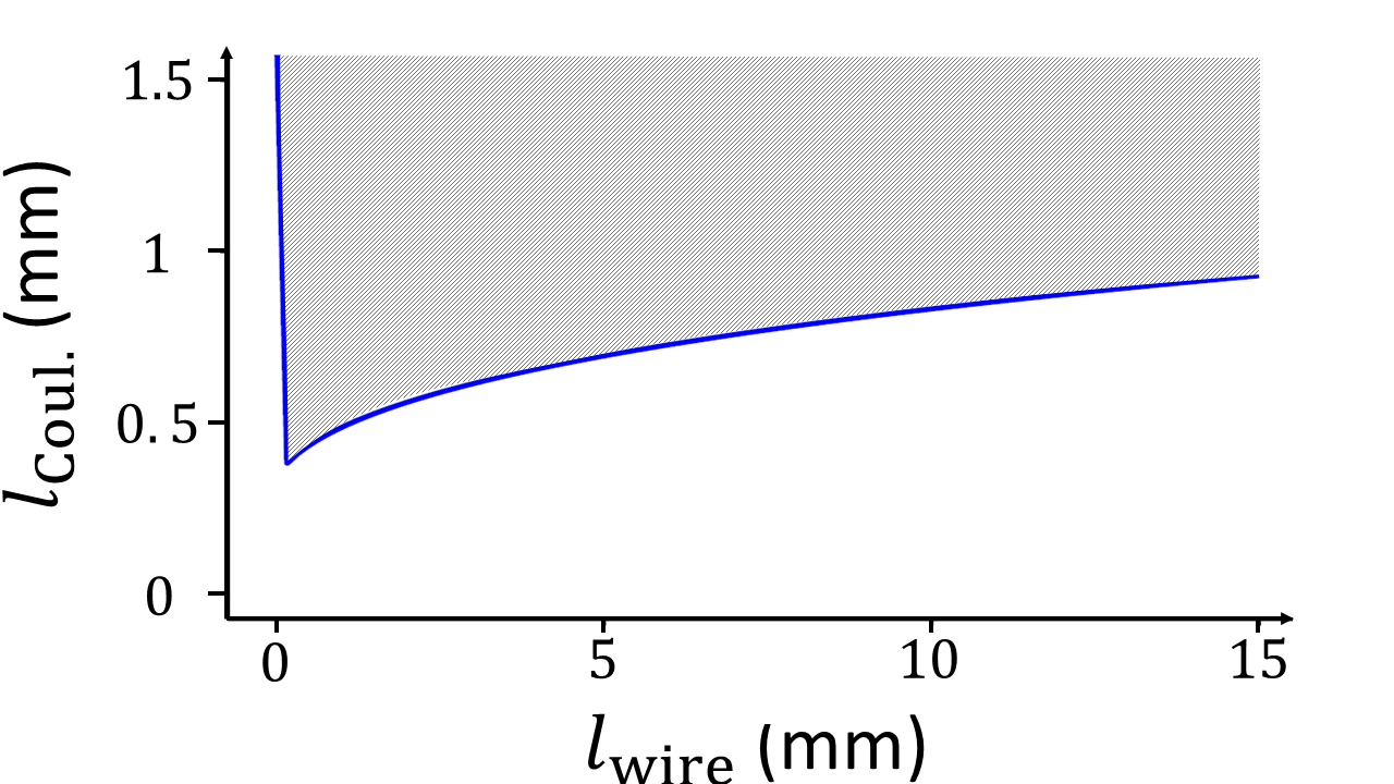
Figure 10: Wire lengths $l_{\mathrm{wire}}$ and ion separations $l_{\mathrm{Coul.}}$ which satisfy $\gamma/\gamma_{\mathrm{Coul.}}\geq 10$. The shaded region shows combinations of $l_{\mathrm{Coul.}}$ and $l_{\mathrm{wire}}$ that satisfy the inequality $\gamma\geq 10\times\gamma_{\mathrm{Coul.}}$

Figure 10 can be used as follows. First, pick a value for $l_{\mathrm{wire}}$, for example $10~{}$mm. Then draw a vertical line upwards until it intersects with the curve. All values of $l_{\mathrm{Coul.}}$ in the shaded region above the point of intersection satisfy $\gamma\geq 10\times\gamma_{\mathrm{Coul.}}$. To give an example, suppose $d=50\times 10^{-6}~{}$m and $l_{\mathrm{Coul.}}\geq 0.5~{}$mm so that decoherence occurs more quickly than state exchange via the direct Coulomb interaction. For instance, we may choose $l_{\mathrm{Coul.}}=1~{}$mm. Next, suppose we want to use a wire of length $l_{\mathrm{wire}}=10~{}$mm. Looking at figure 10 we see that if $l_{\mathrm{Coul.}}$ is greater than about $0.8~{}$mm, the condition $\gamma\geq 10\times\gamma_{\mathrm{Coul.}}$ is satisfied. Due to the physical layout of the coupling system, if $l_{\mathrm{wire}}=10~{}$mm the actual value of $l_{\mathrm{Coul.}}$ will also be about $l_{\mathrm{Coul.}}\approx 10~{}$mm, which means the criterion $\gamma\geq 10\times\gamma_{\mathrm{Coul.}}$ will be satisfied. In this scenario where $l_{\mathrm{Coul.}}\geq 0.8~{}$mm and $l_{\mathrm{Coul.}}\geq 0.5~{}$mm, if state exchange is observed between two ions, one can be confident that the state exchange is mediated by the coupling system rather than the direct Coulomb interaction.

With the coupling system described herein, the distance $l_{\mathrm{Coul.}}$ will in general be approximately equal to $l_{\mathrm{wire}}$. Following the procedure above, the cutoff on $l_{\mathrm{Coul.}}$ is nearly always smaller than $l_{\mathrm{wire}}$. This indicates that for most choices of $l_{\mathrm{wire}}$ the criterion $\gamma\geq 10\times\gamma_{\mathrm{Coul.}}$ is automatically satisfied. The one notable exception is when $l_{\mathrm{wire}}$ approaches the wire radius $a$ and the bound on $l_{\mathrm{Coul.}}$ diverges as shown in figure 10. This unrealistic artifact comes from a limitation in the expression for the capacitance of a finite cylindrical wire, which diverges when the wire radius $a$ approaches the wire length $l_{\mathrm{wire}}$. It is irrelevant provided $l_{\mathrm{wire}}\gg a$.

Appendix L Literature estimates of the decoherence time $t^{\mathrm{wire}}_{\mathrm{deco.}}$ in the coupling system

Johnson-Nyquist and shot noise can both be expressed in terms of a dissipated power. Some authors Daniilidis et al. (2009) use this to estimate a time in which information traveling from ion#1 to ion#2 will be lost, or in other words, a decoherence time for quantum information inside the wire. To illustrate, the power $P_{\mathrm{J.N.}}$ can be interpreted as an ”average number of phonons per second (of the relevant frequency)” entering the coupling system, or the average time for one phonon to disturb the quantum state. To estimate the decoherence time one can consider the time required for $P_{\mathrm{J.N.}}$ to ”produce” one quantum of motional energy, $hf$. In terms of the noise voltage, $P_{\mathrm{J.N.}}\equiv V^{2}_{\mathrm{J.N.}}/R_{\mathrm{wire}}$. From section III.1 we recall that $V_{\mathrm{J.N.}}=\sqrt{4k_{\mathrm{B}}TR_{\mathrm{wire}}\Delta f}$. At $T=10~{}$K with a resistance $R_{\mathrm{wire}}=0.00001~{}\Omega$ and a frequency bandwidth $\Delta f=500~{}$Hz, we find $V_{\mathrm{J.N.}}=1.7\times 10^{-12}~{}$V and hence $P_{\mathrm{J.N.}}\sim 2.8\times 10^{-19}~{}$J/s. For this power, the time needed to create one quantum of noise is $t^{\mathrm{wire}}_{\mathrm{deco.}}=hf/P_{\mathrm{J.N.}}=2.4\times 10^{-8}~{}$s, where $h$ is Plank’s constant. This is far less than the best (shortest) exchange times $t_{\mathrm{ex.}}$ calculated for the coupling system herein. Although the calculated decoherence time $t^{\mathrm{wire}}_{\mathrm{deco.}}$ should correlate with the rate at which the quantum state is disrupted by disturbances from the coupling system, it is not clear how successfully the process of decoherence is captured by a simple model in which noise fluctuations inject an effective power. If similar logic is applied to calculate exchange times assuming an exchange power $P_{\mathrm{ex.}}=V^{2}_{\mathrm{sig.}}/R_{\mathrm{wire}}$ and using the signal strength $V_{\mathrm{sig.}}=4.1\times 10^{-10}~{}$V from table 4, we find excessively short exchange times $t_{\mathrm{ex.}}=hf/P_{\mathrm{ex.}}=3.9\times 10^{-13}~{}$s.

Reference Kotler et al. (2017) outlines an alternative approach for estimating the decoherence time $t^{\mathrm{wire}}_{\mathrm{deco.}}$. The quality factor for an electrical resonator can be rewritten as $\Delta\omega=\omega/{Q}~{}$, which is the range of frequencies to which a resonator is sensitive, or in a sense, its ”linewidth”. When a damped resonator is excited, the characteristic time for the system to relax (ring down) is $t_{\mathrm{thermal}}=1/\left(\Delta\omega\right)=Q/\omega$. At thermal equilibrium the average number of phonons is given by the Bose-Einstein distribution $\bar{n}=\left[\mathrm{exp}(\hbar\omega/k_{\mathrm{B}}T)-1\right]^{-1}$. We now assume the time for the excited resonator to relax to thermal equilibrium, is the same as the time for the system to relax from an average phonon number $\bar{n}=0$, to the thermal equilibrium phonon number $\bar{n}=\left[\mathrm{exp}(\hbar\omega/k_{\mathrm{B}}T)-1\right]^{-1}$. If this is true, the average rate at which phonons must enter the system during the relaxation process is $\bar{n}/t_{\mathrm{thermal}}$ phonons per second. This can be used to define a coherence time

$$1/t^{\mathrm{wire}}_{\mathrm{deco.}}\equiv\bar{n}/t_{\mathrm{thermal}}~{}.$$ (101)

At high temperatures $\left(k_{\mathrm{B}}T\gg\hbar\omega\right)$ the Bose-Einstein distribution reduces to $\bar{n}\approx k_{\mathrm{B}}T/\hbar\omega$, so substituting $\bar{n}$ and $t_{\mathrm{thermal}}$ from above into equation 101 gives $t^{\mathrm{wire}}_{\mathrm{deco.}}\approx\hbar Q/k_{\mathrm{B}}T$. At a lower temperature, $\bar{n}=1$, the coherence time is $t^{\mathrm{wire}}_{\mathrm{deco.}}=t_{\mathrm{thermal}}=Q/\omega$. For a motional mode frequency $f=60~{}$MHz the energy of a quantum of oscillation is $E_{\mathrm{ion}}=hf\sim 4\times 10^{-26}~{}$J where $h$ is Plank’s constant. At a temperature $T=3~{}$K the thermal energy is $E_{\mathrm{temp.}}=k_{\mathrm{B}}T\sim 4\times 10^{-23}~{}$J. In this regime $k_{\mathrm{B}}T\gg hf$, so the decoherence time is $t^{\mathrm{wire}}_{\mathrm{deco.}}\approx\hbar Q/k_{\mathrm{B}}T$. Erickson et al. (2014) report a Q-factor of Q $>10^{7}$ for a resonator at $60~{}$MHz and $T=3~{}$K, using a wire $2~{}\mu$m wide and $25~{}$cm long Erickson et al. (2014). Using this Q-factor gives $t^{\mathrm{wire}}_{\mathrm{deco.}}\sim 2.5\times 10^{-5}~{}$s. This value seems more realistic than the value calculated using the model of an effective noise power injected into the coupling wire, but the second model may still be oversimplified. It is not clear why the time for a damped excited resonator to relax (”cool down”) should be the same as the time for a resonator with zero motional quanta to relax (”heat up”) to thermal equilibrium.

References

- Gaebler et al. (2016) J. P. Gaebler, T. R. Tan, Y. Lin, Y. Wan, R. Bowler, A. C. Keith, S. Glancy, K. Coakley, E. Knill, D. Leibfried, et al., Physical review letters 117, 060505 (2016).
- Harty et al. (2014) T. Harty, D. Allcock, C. J. Ballance, L. Guidoni, H. Janacek, N. Linke, D. Stacey, and D. Lucas, Physical review letters 113, 220501 (2014).
- Noguchi et al. (2020) A. Noguchi, A. Osada, S. Masuda, S. Kono, K. Heya, S. P. Wolski, H. Takahashi, T. Sugiyama, D. Lachance-Quirion, and Y. Nakamura, arXiv preprint arXiv:2005.02630 (2020).
- Barends et al. (2014) R. Barends, J. Kelly, A. Megrant, A. Veitia, D. Sank, E. Jeffrey, T. C. White, J. Mutus, A. G. Fowler, B. Campbell, et al., Nature 508, 500 (2014).
- Bruzewicz et al. (2019) C. D. Bruzewicz, J. Chiaverini, R. McConnell, and J. M. Sage, Applied Physics Reviews 6, 021314 (2019).
- Schäfer et al. (2018) V. Schäfer, C. Ballance, K. Thirumalai, L. Stephenson, T. Ballance, A. Steane, and D. Lucas, Nature 555, 75 (2018).
- Ballance et al. (2016) C. Ballance, T. Harty, N. Linke, M. Sepiol, and D. Lucas, Physical review letters 117, 060504 (2016).
- Wong-Campos et al. (2017) J. Wong-Campos, S. Moses, K. Johnson, and C. Monroe, Physical Review Letters 119, 230501 (2017).
- Oliver and Welander (2013) W. D. Oliver and P. B. Welander, MRS bulletin 38, 816 (2013).
- Rigetti et al. (2012) C. Rigetti, J. M. Gambetta, S. Poletto, B. Plourde, J. M. Chow, A. Córcoles, J. A. Smolin, S. T. Merkel, J. Rozen, G. A. Keefe, et al., Physical Review B 86, 100506 (2012).
- Brown et al. (2016) K. R. Brown, J. Kim, and C. Monroe, npj Quantum Information 2, 1 (2016).
- Landsman et al. (2019a) K. A. Landsman, Y. Wu, P. H. Leung, D. Zhu, N. M. Linke, K. R. Brown, L. Duan, and C. Monroe, Physical Review A 100, 022332 (2019a).
- Kaufmann et al. (2014) H. Kaufmann, T. Ruster, C. Schmiegelow, F. Schmidt-Kaler, and U. Poschinger, New Journal of Physics 16, 073012 (2014).
- Kaushal et al. (2020) V. Kaushal, B. Lekitsch, A. Stahl, J. Hilder, D. Pijn, C. Schmiegelow, A. Bermudez, M. Müller, F. Schmidt-Kaler, and U. Poschinger, AVS Quantum Science 2, 014101 (2020).
- Wan et al. (2020) Y. Wan, R. Jördens, S. Erickson, J. Wu, R. Bowler, T. Tan, P.-Y. Hou, D. Wineland, A. Wilson, and D. Leibfried, arXiv preprint arXiv:2003.03520 (2020).
- Pino et al. (2020) J. Pino, J. Dreiling, C. Figgatt, J. Gaebler, S. Moses, C. Baldwin, M. Foss-Feig, D. Hayes, K. Mayer, C. Ryan-Anderson, et al., arXiv preprint arXiv:2003.01293 (2020).
- Landsman et al. (2019b) K. A. Landsman, Y. Wu, P. H. Leung, D. Zhu, N. M. Linke, K. R. Brown, L. Duan, and C. Monroe, Physical Review A 100, 022332 (2019b).
- Stute et al. (2012) A. Stute, B. Casabone, P. Schindler, T. Monz, P. Schmidt, B. Brandstätter, T. Northup, and R. Blatt, Nature 485, 482 (2012).
- Monroe et al. (2014) C. Monroe, R. Raussendorf, A. Ruthven, K. Brown, P. Maunz, L.-M. Duan, and J. Kim, Physical Review A 89, 022317 (2014).
- Heinzen and Wineland (1990) D. Heinzen and D. Wineland, Physical Review A 42, 2977 (1990).
- Daniilidis et al. (2009) N. Daniilidis, T. Lee, R. Clark, S. Narayanan, and H. Häffner, Journal of Physics B: Atomic, Molecular and Optical Physics 42, 154012 (2009).
- Zurita-Sánchez and Henkel (2008) J. R. Zurita-Sánchez and C. Henkel, New Journal of Physics 10, 083021 (2008).
- Marzoli et al. (2009) I. Marzoli, P. Tombesi, G. Ciaramicoli, G. Werth, P. Bushev, S. Stahl, F. Schmidt-Kaler, M. Hellwig, C. Henkel, G. Marx, et al., Journal of Physics B: Atomic, Molecular and Optical Physics 42, 154010 (2009).
- Liang and Ke-Lin (2010) C. Liang and G. Ke-Lin, Chinese Physics B 19, 110309 (2010).
- Kotler et al. (2017) S. Kotler, R. W. Simmonds, D. Leibfried, and D. J. Wineland, Physical Review A 95, 022327 (2017).
- Rica et al. (2018) R. A. Rica, F. Domínguez, M. J. Gutiérrez, J. Bañuelos, J. J. del Pozo, and D. Rodríguez, The European Physical Journal Special Topics 227, 445 (2018).
- DiVincenzo (2000) D. P. DiVincenzo, Fortschritte der Physik: Progress of Physics 48, 771 (2000).
- Schmidt-Kaler et al. (2003) F. Schmidt-Kaler, S. Gulde, M. Riebe, T. Deuschle, A. Kreuter, G. Lancaster, C. Becher, J. Eschner, H. Häffner, and R. Blatt, Journal of Physics B: Atomic, Molecular and Optical Physics 36, 623 (2003).
- Deslauriers et al. (2006) L. Deslauriers, S. Olmschenk, D. Stick, W. Hensinger, J. Sterk, and C. Monroe, Physical Review Letters 97, 103007 (2006).
- Epstein et al. (2007) R. Epstein, S. Seidelin, D. Leibfried, J. Wesenberg, J. J. Bollinger, J. Amini, R. Blakestad, J. Britton, J. Home, W. M. Itano, et al., Physical Review A 76, 033411 (2007).
- Lucas et al. (2007) D. Lucas, B. Keitch, J. Home, G. Imreh, M. McDonnell, D. Stacey, D. Szwer, and A. Steane, arXiv preprint arXiv:0710.4421 (2007).
- Labaziewicz et al. (2008) J. Labaziewicz, Y. Ge, D. R. Leibrandt, S. X. Wang, R. Shewmon, and I. L. Chuang, Physical review letters 101, 180602 (2008).
- Hite et al. (2012) D. A. Hite, Y. Colombe, A. C. Wilson, K. R. Brown, U. Warring, R. Jördens, J. D. Jost, K. McKay, D. Pappas, D. Leibfried, et al., Physical review letters 109, 103001 (2012).
- Chiaverini and Sage (2014) J. Chiaverini and J. Sage, Physical Review A 89, 012318 (2014).
- Daniilidis et al. (2014) N. Daniilidis, S. Gerber, G. Bolloten, M. Ramm, A. Ransford, E. Ulin-Avila, I. Talukdar, and H. Häffner, Physical Review B 89, 245435 (2014).
- Bruzewicz et al. (2015) C. Bruzewicz, J. Sage, and J. Chiaverini, Physical Review A 91, 041402 (2015).
- Talukdar et al. (2016) I. Talukdar, D. Gorman, N. Daniilidis, P. Schindler, S. Ebadi, H. Kaufmann, T. Zhang, and H. Häffner, Physical Review A 93, 043415 (2016).
- Sedlacek et al. (2018a) J. Sedlacek, A. Greene, J. Stuart, R. McConnell, C. Bruzewicz, J. Sage, and J. Chiaverini, Physical Review A 97, 020302 (2018a).
- Sedlacek et al. (2018b) J. Sedlacek, J. Stuart, D. H. Slichter, C. Bruzewicz, R. McConnell, J. Sage, and J. Chiaverini, Physical Review A 98, 063430 (2018b).
- An et al. (2019) D. An, C. Matthiesen, E. Urban, and H. Häffner, Physical Review A 100, 063405 (2019).
- Griffiths (1962a) D. J. Griffiths, Introduction to electrodynamics (Prentice Hall New Jersey, 1962).
- Griffiths (1962b) D. J. Griffiths, “Introduction to electrodynamics,” (Prentice Hall New Jersey, 1962) Chap. 3, pp. 121–123, 3rd ed., the international version with Chinese writing on the cover.
- Daniilidis and Häffner (2013) N. Daniilidis and H. Häffner, Annu. Rev. Condens. Matter Phys. 4, 83 (2013).
- Young et al. (2007a) H. D. Young, R. A. Freedman, and L. Ford, “University physics vol 2 (chapters 21-37),” (Pearson education, 2007) Chap. 31, p. 1063, 12th ed.
- McDonald (2003) K. T. McDonald, “Capacitance of a thin conducting disk and of conducting spheroids,” (2003).
- (46) richard.ness@nessengr.com, “Skin depth/skin effect and calculator,” www.nessengr.com/technical-data/skin-depth/, accessed February 12, 2019.
- Young et al. (2007b) H. D. Young, R. A. Freedman, and L. Ford, “University physics vol 2 (chapters 21-37),” (Pearson education, 2007) Chap. 21, p. 730, 12th ed.
- Sorensen et al. (2004) A. S. Sorensen, C. H. van der Wal, L. I. Childress, and M. D. Lukin, Physical review letters 92, 063601 (2004).
- Bohman et al. (2018) M. Bohman, A. Mooser, G. Schneider, N. Schön, M. Wiesinger, J. Harrington, T. Higuchi, H. Nagahama, C. Smorra, S. Sellner, et al., Journal of Modern Optics 65, 568 (2018).
- Wineland and Dehmelt (1975) D. Wineland and H. Dehmelt, Journal of Applied Physics 46, 919 (1975).
- Van Horne and Mukherjee (2020a) N. Van Horne and M. Mukherjee, arXiv preprint arXiv:2008.07128 (2020a).
- Portes et al. (2008) D. Portes, H. Rodrigues, S. Duarte, and B. Baseia, The European Physical Journal D 48, 145 (2008).
- Estes et al. (1968) L. E. Estes, T. H. Keil, and L. M. Narducci, Physical Review 175, 286 (1968).
- Leibfried et al. (2003) D. Leibfried, R. Blatt, C. Monroe, and D. Wineland, Reviews of Modern Physics 75, 281 (2003), section III, Trapped two-level atoms coupled to light fields.
- Griffiths (1962c) D. J. Griffiths, “Introduction to electrodynamics,” (Prentice Hall New Jersey, 1962) Chap. 2,3, 3rd ed., see potential of an infinite wire above a grounded plane e.g. solutions to prbs 2.47 or 3.9.
- Lundberg (2002) K. H. Lundberg, Unpublished paper 3, 28 (2002).
- Kogan (2008) S. Kogan, Electronic noise and fluctuations in solids (Cambridge University Press, 2008).
- Blanter and Büttiker (2000a) Y. M. Blanter and M. Büttiker, Physics reports 336, 1 (2000a), the relevant information is found in one of the following sections: 1.3 or 1.4 or 2.4.
- (59) www.fis.unipr.it/~gigi/dida/strumentazione/harvard_noise.pdf, appendix A and Appendix B. Accessed February 08, 2020.
- Johnson et al. (2016) K. Johnson, J. Wong-Campos, A. Restelli, K. Landsman, B. Neyenhuis, J. Mizrahi, and C. Monroe, Review of Scientific Instruments 87, 053110 (2016).
- Matula (1979) R. A. Matula, Journal of Physical and Chemical Reference Data 8, 1147 (1979), see table 2, page 1161 of the document.
- Ulmer et al. (2009) S. Ulmer, H. Kracke, K. Blaum, S. Kreim, A. Mooser, W. Quint, C. C. Rodegheri, and J. Walz, Review of Scientific Instruments 80, 123302 (2009).
- Erickson et al. (2014) R. P. Erickson, M. R. Vissers, M. Sandberg, S. R. Jefferts, and D. P. Pappas, Physical review letters 113, 187002 (2014).
- (64) www.fis.unipr.it/~gigi/dida/strumentazione/harvard_noise.pdf, accessed February 08, 2020, Clear derivation, Appendix C.
- Schottky (1918) W. Schottky, Annalen der physik, Original version, in German 362, 541 (1918).
- Schottky (2018) W. Schottky, Journal of Micro/Nanolithography, MEMS, and MOEMS, English translation 17, 041001 (2018).
- Landauer (1957) R. Landauer, IBM Journal of research and development 1, 223 (1957).
- Li et al. (1990) Y. P. Li, D. C. Tsui, J. J. Heremans, J. Simmons, and G. Weimann, Applied physics letters 57, 774 (1990).
- Blanter and Büttiker (2000b) Y. M. Blanter and M. Büttiker, Physics reports 336, 1 (2000b), section 4, Shot noise in hybrid normal and superconducting structures (in introduction).
- Ostrove and Reichl (2019) C. Ostrove and L. E. Reichl, Physica B: Condensed Matter 561, 79 (2019).
- Büttiker (1992) M. Büttiker, Physical Review B 45, 3807 (1992).
- Chen and Ting (1991) L. Chen and C. Ting, Physical Review B 43, 4534 (1991).
- Schoelkopf et al. (1997) R. Schoelkopf, P. Burke, A. Kozhevnikov, D. Prober, and M. Rooks, Physical review letters 78, 3370 (1997).
- Turchette et al. (2000) Q. A. Turchette, B. King, D. Leibfried, D. Meekhof, C. Myatt, M. Rowe, C. Sackett, C. Wood, W. Itano, C. Monroe, et al., Physical Review A 61, 063418 (2000).
- Brownnutt et al. (2015) M. Brownnutt, M. Kumph, P. Rabl, and R. Blatt, Reviews of modern Physics 87, 1419 (2015).
- Lau et al. (2001) C. N. Lau, N. Markovic, M. Bockrath, A. Bezryadin, and M. Tinkham, Physical review letters 87, 217003 (2001).
- Chiaverini et al. (2005) J. Chiaverini, R. Blakestad, J. Britton, J. Jost, C. Langer, D. Leibfried, R. Eri, and D. Wineland, Quantum Information and Computation 5, 419 (2005).
- Wineland et al. (2005) D. J. Wineland, D. Leibfried, M. D. Barrett, A. Ben-Kish, J. C. Bergquist, R. Blakestad, J. J. Bollinger, J. Britton, J. Chiaverini, B. DeMarco, et al., in Laser Spectroscopy (World Scientific, 2005) pp. 393–402.
- Stick et al. (2006) D. Stick, W. Hensinger, S. Olmschenk, M. Madsen, K. Schwab, and C. Monroe, Nature Physics 2, 36 (2006).
- Boldin et al. (2018) I. A. Boldin, A. Kraft, and C. Wunderlich, Physical review letters 120, 023201 (2018).
- Savard et al. (1997) T. Savard, K. O’hara, and J. Thomas, Physical Review A 56, R1095 (1997).
- Walther et al. (2012) A. Walther, F. Ziesel, T. Ruster, S. T. Dawkins, K. Ott, M. Hettrich, K. Singer, F. Schmidt-Kaler, and U. Poschinger, Physical review letters 109, 080501 (2012).
- Hansen (2006) R. C. Hansen, Electrically small, superdirective, and superconducting antennas (John Wiley & Sons, 2006).
- Kleczewski et al. (2012) A. Kleczewski, M. R. Hoffman, J. Sherman, E. Magnuson, B. B. Blinov, and E. Fortson, Physical Review A 85, 043418 (2012).
- Bezryadin et al. (2000) A. Bezryadin, C. Lau, and M. Tinkham, Nature 404, 971 (2000).
- Safronova et al. (2014) M. Safronova, V. Dzuba, V. Flambaum, U. Safronova, S. Porsev, and M. Kozlov, Physical review letters 113, 030801 (2014).
- Tra (a) “What is a transmission line?” https://www.allaboutcircuits.com/textbook/radio-frequency-analysis-design/real-life-rf-signals/what-is-a-transmission-line/ (a), chapter 3 - Real-Life RF Signals. Accessed February 02, 2020.
- Tra (b) https://en.wikipedia.org/wiki/Transmission_line (b), section: Applicability. Accessed February 02, 2020.
- Mi et al. (2018) X. Mi, M. Benito, S. Putz, D. M. Zajac, J. M. Taylor, G. Burkard, and J. R. Petta, Nature 555, 599 (2018).
- Zurita-Sánchez and Henkel (2006) J. R. Zurita-Sánchez and C. Henkel, Physical Review A 73, 063825 (2006).
- Weingarten (1996) W. Weingarten, (1996).
- (92) https://en.wikipedia.org/wiki/Superconducting_radio_frequency, accessed February 03, 2020.
- Boogaard et al. (2004) G. Boogaard, A. Verbruggen, W. Belzig, and T. M. Klapwijk, Physical Review B 69, 220503 (2004).
- Dressel (2013) M. Dressel, Advances in Condensed Matter Physics 2013 (2013).
- Van Horne and Mukherjee (2020b) N. Van Horne and M. Mukherjee, arXiv preprint arXiv:2011.09777 (2020b).
- McDonald (2002) K. T. McDonald, Princeton Univ., Princeton, NJ.[Online]. Available: http://puhep1. princeton. edu/~ mcdonald/examples/ellipsoid. pdf (2002).
- Thomson (Lord Kelvin) W. Thomson (Lord Kelvin), “Papers on electrostatics and magnetism,” (Macmillan, London, 1884) pp. 7 and 178–179, 2nd ed., reprint of Papers on Electrostatics and Magnetism: by Sir William Thomson Kelvin, William Thomson, 1824-1907, and Burndy Library.
- Jackson (1999) J. D. Jackson, “Classical electrodynamics,” (Wiley, New York, 1999) pp. sec. 2.11, pg 78, 3rd ed., in figure 2.13.
- (99) https://en.wikipedia.org/wiki/Nanowire, section: Conductivity of nanowires. Accessed February 08, 2020.
- (100) https://physics.nist.gov/cgi-bin/cuu/Value?eqconqu2e2sh, accessed February 08, 2020.
- Shockley (1938) W. Shockley, Journal of applied physics 9, 635 (1938).
- Sirkis and Holonyak Jr (1966) M. D. Sirkis and N. Holonyak Jr, American Journal of Physics 34, 943 (1966).
- Jackson (2004) R. G. Jackson, Novel sensors and sensing (CRC Press, 2004).
- Daniilidis et al. (2011) N. Daniilidis, S. Narayanan, S. A. Möller, R. Clark, T. E. Lee, P. J. Leek, A. Wallraff, S. Schulz, F. Schmidt-Kaler, and H. Häffner, New Journal of Physics 13, 013032 (2011).
- Noel et al. (2019) C. Noel, M. Berlin-Udi, C. Matthiesen, J. Yu, Y. Zhou, V. Lordi, and H. Häffner, Physical Review A 99, 063427 (2019).
- Lamoreaux (1997) S. Lamoreaux, Physical Review A 56, 4970 (1997).
- Henkel et al. (1999) C. Henkel, S. Pötting, and M. Wilkens, Applied Physics B 69, 379 (1999).
- Safavi-Naini et al. (2011) A. Safavi-Naini, P. Rabl, P. Weck, and H. Sadeghpour, Physical Review A 84, 023412 (2011).
- Safavi-Naini et al. (2013) A. Safavi-Naini, E. Kim, P. Weck, P. Rabl, and H. Sadeghpour, Physical Review A 87, 023421 (2013).
- Daniilidis and Häffner (2011) N. Daniilidis and H. Häffner, Physics 4, 66 (2011).
- McRae et al. (2018) C. McRae, J. Béjanin, C. Earnest, T. McConkey, J. Rinehart, C. Deimert, J. Thomas, Z. Wasilewski, and M. Mariantoni, Journal of Applied Physics 123, 205304 (2018).
- Righini et al. (2011) G. Righini, Y. Dumeige, P. Feron, M. Ferrari, G. Nunzi Conti, D. Ristic, and S. Soria, La Rivista del Nuovo Cimento 34, 435 (2011).
- Allcock et al. (2011) D. Allcock, L. Guidoni, T. Harty, C. Ballance, M. Blain, A. Steane, and D. Lucas, New Journal of Physics 13, 123023 (2011).
- Van Horne et al. (2020) N. Van Horne, D. Yum, T. Dutta, P. Hänggi, J. Gong, D. Poletti, and M. Mukherjee, npj Quantum Information 6, 1 (2020).
- Wineland et al. (1998) D. J. Wineland, C. Monroe, W. M. Itano, D. Leibfried, B. E. King, and D. M. Meekhof, Journal of research of the National Institute of Standards and Technology 103, 259 (1998).
- Brown et al. (2011) K. R. Brown, C. Ospelkaus, Y. Colombe, A. C. Wilson, D. Leibfried, and D. J. Wineland, Nature 471, 196 (2011).