Morph Detection Enhanced by Structured Group Sparsity
Abstract
In this paper, we consider the challenge of face morphing attacks, which substantially undermine the integrity of face recognition systems such as those adopted for use in border protection agencies. Morph detection can be formulated as extracting fine-grained representations, where local discriminative features are harnessed for learning a hypothesis. To acquire discriminative features at different granularity as well as a decoupled spectral information, we leverage wavelet domain analysis to gain insight into the spatial-frequency content of a morphed face. As such, instead of using images in the RGB domain, we decompose every image into its wavelet sub-bands using 2D wavelet decomposition and a deep supervised feature selection scheme is employed to find the most discriminative wavelet sub-bands of input images. To this end, we train a Deep Neural Network (DNN) morph detector using the decomposed wavelet sub-bands of the morphed and bona fide images. In the training phase, our structured group sparsity-constrained DNN picks the most discriminative wavelet sub-bands out of all the sub-bands, with which we retrain our DNN, resulting in a precise detection of morphed images when inference is achieved on a probe image. The efficacy of our deep morph detector which is enhanced by structured group lasso is validated through experiments on three facial morph image databases, i.e., VISAPP17, LMA, and MorGAN.
1 INTRODUCTION
Face forgery detection has gained momentum recently in the biometric community owing to its vast application, especially in commercial face recognition systems [27, 19, 53, 37, 18, 10]. Photo-realistic forged images tamper with the functionality and integrity of security checkpoints, where, ideally, there must be a zero-tolerance policy to false acceptance [24, 51, 12, 40]. Introduced in [12], facial morph images, as one of the categories of the forged face images, can bypass established automated face recognition systems, as well as border control officers, where both struggle to distinguish a bona fide image from a morphed one [25] due to delicacy in synthesizing morphed samples. Face morphing attacks are synthesized using two look-alike genuine images, for example one representing a criminal and one for an innocent subject, in which the final morphed image can be verified against both subjects. Two underlying genuine images are sampled from two distributions, and the resulting morphed sample is characterized using the blended features of the two genuine images. If we assume the support of high-dimensional genuine and morphed samples are two underlying embedding low-dimensional manifolds, morphed samples are intentionally crafted near the discriminating boundary of the two manifolds, which justifies its verifiability against both real subjects.
Face morphing attacks are forged in either the image domain or in the latent domain. In image domain morphing, two genuine images are translated into a set of aligned averaged landmarks and a morphed sample is synthesized after warping and alpha blending. In latent space morphing, a generative adversarial network, which has an attached encoder, first captures the distribution of genuine images, and converts two genuine images into two latent vectors that can be mixed using the convex combination of both vectors. From the detection standpoint, previous research efforts have considered two approaches to detect morphed samples. Single morphed image detection, which is the focus of this study, labels an image as either genuine (negative) or morphed (positive). On the other hand, differential morph detection employs a probe image and an auxiliary one, which is usually a live photo of a subject, to define morph detection framework.
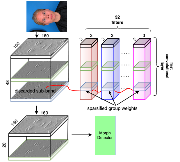
Deep learning-based techniques have shown compelling results for detecting morphed images through harnessing representation learning [7] by mapping data samples into an embedding space where the separability between genuine and morphed samples is guaranteed through the aligning parameter space of a Deep Neural Network (DNN). Since the discrepancies between a bona fide and its corresponding morphed image are subtle and local, fine-grained feature learning [16, 53] can be tailored for our morph detection algorithm. To mitigate the curse of dimensionality, feature selection is a powerful tool to find the most discriminating hyperplane in a binary classification setting. A DNN can pick the most discriminative structured group features of its input space by adjusting its kernel parameters used in its first convolutional layer. Enforcing a group sparsity constraint over the weights of the first convolutional layer in a DNN through the manipulation of its loss function can guide the parameter space to convergence on a set of parameters that picks the most discriminative channels of input data (see Figure 1).
In this work, we tackle single image morph detection. Inspired by the aforementioned feature selection scheme, we investigate the application of group-L1 sparsity [47] over the weights of the first convolutional layer in a DNN as the criterion for selecting the most discriminative input samples’ wavelet sub-bands. Discriminative wavelet sub-bands, which can be thought of as fine-grained features, are learned during the training of our DNN, guaranteeing that an optimal hyperplane will be found between genuine and morphed samples. We conduct experiments on three morph image datasets, i.e., VISAPP17 [23], LMA [9], and MorGAN [9]. Given supervised data samples, our DNN sparsifies the kernel parameters of the first convolutional layer on-the-fly while training, which drives our sparsity-guided DNN into detecting morphed samples.
2 RELATED WORKS
2.1 Morph Generation
The landmark based image morphing technique [23, 9, 38, 12] considers the geometry of two bona fide subjects for generating a morphed sample. Every pixel location in both genuine images is warped to preserve the correspondence in the resulting morphed sample, and a convex combination of the warped pixels cross-dissolve the warped pixels in the real images to synthesize that pixel location in the final morphed sample. On the other hand, Generative Adversarial Network (GAN)-based image morphing techniques focus on the distribution of real images. A trained GAN is able to find the distribution where data samples are drawn from. The point here is that a convex combination is generated in the latent domain . Since GANs do not map an image into a latent vector , an encoder attached to the generator of a GAN can achieve this mapping. A trained GAN maps two genuine images into a latent domain for interpolation, and a decoder maps the interpolated vector into the image domain to realize morphed samples [9, 1].
2.2 Morph Detection
Different methods have been proposed for morph detection [36, 3, 33, 41, 35, 14, 4, 45], some of which are discussed here. Ferrara et al. [13] introduced face demorphing to reverse the morphing process to detect altered images. Some research considers hand-crafted descriptors to detect morphed samples [11, 29, 34, 28], where the fusion of different features has proven to be compelling for morph detection [34, 32]. Deep morph detectors utilize the power of convolutional neural networks to detect morphed samples accurately [14, 30, 37, 38, 36, 22]. Several studies investigate denoising methods for the task of morph attack detection. In [31], Photo Response Non-Uniformity (PRNU) is investigated as an indicator to distinguish a bona fide sample from a morphed one. It is shown in [31] that morphed samples exhibit a distinguishing spectral response compared to the response related to bona fide images. In [46], the residual noise of an image is utilized to extract deep features for training a morph detector. In [2], to increase the accuracy of morph detection, a soft attention mechanism is adopted to steer the focus of a DNN into the most discriminative spatial regions in an image under investigation. In [8], a GAN-based single image morph discriminator is trained, which leverages adversarial learning to detect single image morphing attacks.
2.3 Selecting Structured Features
Feature selection is one of the most useful tools for classification, and finding relevant features that have the maximum mutual information with the predictor’s output is highly desirable. When features are arranged in a group setting, group Lasso [50], as one of the many feature selection methods, has shown impressive proficiency [52, 48, 47, 49, 15]. When the -norm of some structured parameters, such as grouped weights in a convolutional layer of a DNN, are added to the objective function in an optimization framework, which is known as Lasso regularization [43], sparsified grouped parameters leads to feature selection, which is known as structured group sparsity in a DNN [47].
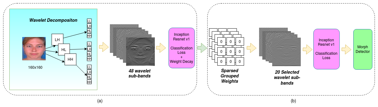
(b): We retrain our modified DNN using the 20 discriminative wavelet sub-bands, where the input channel size of our DNN is reduced to 20. A binary classifier is learned for morph detection.
3 PROPOSED FRAMEWORK
To incorporate fine-grained spatial-frequency features into our proposed framework, we leverage wavelet domain analysis as the basis of our deep morph detector. At varied granularity, wavelet sub-bands contain local discriminative information, where morphing artifacts are uncovered in this domain. Our wavelet-based deep morph detection mechanism is two-fold. First, we accomplish the sub-band selection to find the most informative subset of features to increase the confidence of our deep morph detector as far as inference is concerned. As presented in Figure 1, the optimization framework in the structured group sparsity zeros out the grouped weights corresponding to convolutional filters in a given layer of a DNN morph detector. Once some grouped weights in a convoluational layer converge to zero, those involved wavelet sub-bands are discarded, that is an implicit feature selection method. Secondly, we train our DNN detector using the selected wavelet sub-bands for the task of morph detection (see Figure 2).
3.1 Sub-band Selection Based on Group Lasso
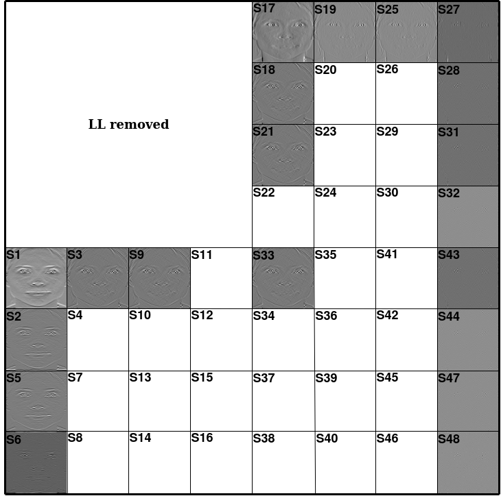
We utilize the valuable spatial-frequency information provided by the wavelet decomposition to enhance the accuracy of our proposed morph detector. We pre-processed every input image using a three-level uniform wavelet decomposition. Since the morphing artifacts are revealed in the high frequency spectra, we discard the Low-Low (LL) sub-band after the first level of decomposition, and the remaining 48 wavelet sub-bands are extracted to be used by our deep morph detector.
Since we intend to select the most discriminative wavelet sub-bands, our focus is on the first convolutional layer of our DNN. Please note that the input consists of wavelet sub-bands (channels) and the first convolutional layer is defined in the space of where and represent the number of filters, number of kernels, height, and width of a kernel, respectively. Here, we differentiate between the filter and the kernel terminologies as discussed in [5]. A kernel is a 2D array of size . A filter is an array of size , which is a 3D structure of stacked 2D kernels. For every input image, we have 48 concatenated wavelet sub-bands as input to our DNN detector, which implies that the number of kernels in each filter of the first convolutional layer is equal to 48. We employ 32 different filters in the first convolutional layer, where the size of each kernel is . Thus, the dimensions of the first convolutional layer in the stage of feature selection are as follows: and . It is worth mentioning that we have 48 different grouped weights that are shown by for c , where the first layer weights are denoted by . Discriminative wavelet sub-bands are selected in accordance with a supervised feature selection algorithm. Our objective is to impose a group sparsity constraint on the parameters of the first convolutional layer in our DNN framework. Adding a structured sparsity regularization penalty to the classification loss of our DNN detector forces our network into sparsifying the grouped weights of the first convolutional layer, which implicitly results in discarding irrelevant wavelet sub-bands, or selecting the most discriminative sub-bands. Thus, only a certain number of informative wavelet sub-bands, out of 48, are selected, with which we train our DNN morph detector.
3.2 Rewriting the Classification Loss of the DNN Detector
If we denote the classification loss of our DNN detector as , the set of parameters of our network as , the first layer weights as , and each grouped weight in the first layer as , the regularized loss function, denoted by , for training the deep neural network is as follows:
| (1) |
where is a set composed of all the group weights of the convolutional filters in the first layer, and is a parameter controlling the amount of sparsity. The regularized loss can be re-written as:
| (2) |
where delineates the binary cross-entropy classification loss and and .
3.3 Learning Deep Morph Detector
Regarding our feature selection scheme, as mentioned in Eqs. 1 and 2, there is a hyperparameter in the optimization framework of our DNN detector, which is the regularization coefficient. To find the optimal regularization coefficient we utilize the validation sets of our datasets. To incorporate all three datasets in the selection process of hyperparameter , we combine all the images in the three datasets, i.e., VISAPP17 [23], LMA [9], and MorGAN [9], and we create a “universal dataset”. A hyperparameter search is performed over different values of . For each value of , our group sparsity-constrained DNN is trained using the training portion of the universal dataset, and the performance of the trained DNN detector is evaluated through Area Under the Curve (AUC) using the validation portion of the universal dataset. The highest AUC corresponds to the optimal value for . Once, we obtained the most discriminative wavelet sub-bands, we retrain our DNN using the selected wavelet sub-bands. Please note that since the number of input wavelet sub-bands is reduced due to feature selection, the number of channels in the filters of the first convolutional layer is also reduced.
4 EVALUATIONS
4.1 Datasets
We employ the VISAPP17 [23], MorGAN [9], and LMA [9] datasets in this work. The VISAPP17 and LMA datasets were generated using facial landmark manipulation techniques, which is an alpha blending of the warped bona fide images. On the other hand, the MorGAN dataset is synthesized using a GAN, including a decoder network that utilizes transposed convolutional layers to transform a convex combination of two generated latent vectors into the image domain. The VISAPP17 dataset has been generated using the images in the Utrecht FCVP dataset, and the LMA and MorGAN datasets were generated using the CelebA dataset [20]. For all images, face detection is performed via MTCNN and all images are resized to . We apply 2D undecimated wavelet decomposition on all images, and since we get 48 concatenated wavelet sub-bands for each image, the dimension of each data sample is .
As for the universal dataset introduced in Section 3.4., the training set includes 1,631 bona fide, and 1,183 morphed images, the validation set consists of 462 bona fide, and 167 morphed samples and the test set includes 1,631 bonafide, and 1,183 morphed images.
4.2 Experimental Setup
We adopt a modified version of the Inception-ResNet-v1 [42] as the backbone of our DNN architecture for learning the discriminative sub-bands, as well as distinguishing morphed samples. We change the number of channels in the first convolutional layer of the Inception-ResNet-v1 to 48 during the sub-band selection stage. As mentioned in Section 3.2., a sample input consists of 48 stacked wavelet sub-bands; thus, the convolutional filters of the first layer have 48 channels, as seen in Figure 1. Inspired by [47], we use group -regularization to impose structured group sparsity constraint on the grouped weight parameters in the first convolutional layer of our deep neural network. For training our modified Inception-ResNet-v1, we adopt the Adam optimizer and training is done for 150 epochs. The learning schedule is as follows: the learning rate is initialized with 0.001, and it is divided by 10 after every 20 epochs. The training phase is accelerated using two 12 GB TITAN X (Pascal) GPUs.
4.3 Evaluation Metrics
We use the APCER, BPCER, and D-EER metrics to assess the performance of our deep morph detector. The first metric, Attack Presentation Classification Error Rate (APCER), is the percentage of morphed images that are classified as bona fide, and the second metric, Bona Fide Presentation Classification Error Rate (BPCER), represents percentage of bona fide samples that are classified as morphed. D-EER stands for Detection Equal Error Rate, at which APCER equals BPCER. The BPCER5 is the BPCER rate when APCER=5%, and similarly the BPCER10 is the BPCER rate when APCER=10%.
| Dataset | Algorithm | D-EER | 5% | 10% |
|---|---|---|---|---|
| VISAPP17 | BSIF+SVM [17] | 16.51 | 35.61 | 26.79 |
| SIFT+SVM [21] | 38.59 | 82.40 | 75.60 | |
| LBP+SVM [26] | 38.00 | 77.10 | 67.90 | |
| SURF+SVM [6] | 30.45 | 84.70 | 69.40 | |
| RGB+DNN [42] | 1.76 | 0.588 | 0.58 | |
| 48-sub-bands | 0.00 | 0.00 | 0.00 | |
| Ours | 0.00 | 0.00 | 0.00 | |
| LMA | BSIF+SVM [17] | 33.05 | 78.34 | 62.86 |
| SIFT+SVM [21] | 33.30 | 83.40 | 72.00 | |
| LBP+SVM [26] | 28.00 | 58.60 | 51.40 | |
| SURF+SVM [6] | 37.40 | 79.50 | 70.00 | |
| RGB+DNN [42] | 9.10 | 15.18 | 7.49 | |
| 48-sub-bands | 5.04 | 4.38 | 2.75 | |
| Ours | 6.80 | 8.60 | 4.89 | |
| MorGAN | BSIF+SVM [17] | 1.57 | 1.42 | 1.30 |
| SIFT+SVM [21] | 43.50 | 93.20 | 84.20 | |
| LBP+SVM [26] | 20.10 | 52.70 | 32.30 | |
| SURF+SVM [6] | 39.95 | 80.00 | 72.60 | |
| RGB+DNN [42] | 2.44 | 1.88 | 1.50 | |
| 48-sub-bands | 0.81 | 0.59 | 0.32 | |
| Ours | 0.42 | 0.38 | 0.22 |
4.4 Tuning the Group Sparsity Regularization Hyperparameter
We performed a search over the group sparsity regularization coefficient . To find the optimal value for , as discussed in Section 3.4., we fine tune our modified Inception-ResNet-v1 DNN [42], already pre-trained on VGGFace2, using the training portion of the universal dataset. For each value of hyperparameter , we trained our modified Inception-ResNet-v1 DNN using the training portion of the universal dataset, and we found the AUC metric when our trained DNN is evaluated using the validation portion of the universal dataset. It should be noted that we created the universal dataset for hyperparameter selection since we wanted to train a morph detector that performs well across different morphing techniques. In addition, after our network is fully trained, we zero out any grouped weight with a weight parameters norm smaller than 0.001. It was found that yields the top 20 most discriminative sub-bands, with the corresponding highest AUC of 99.31%. Figure 3 depicts the selected sub-bands along with the corresponding numbers after training our network using universal dataset, and .
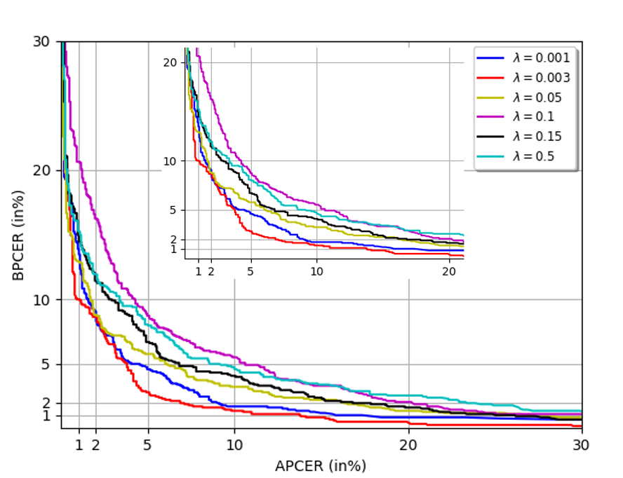
Considering the aforementioned hyperparameter tuning process, we displayed the performance of our morph detector for some selected values of using the validation portion of the universal dataset. Figure 4 shows the Detection Error Trade-off (DET) curves corresponding to different group sparsity regularization parameter . We can clearly see that the performance of our deep morph detector is at its best when .
| Train | Test | Algorithm | D-EER | 5% | 10% |
|---|---|---|---|---|---|
| Universal(VISAPP17+MorGAN+LMA) | VISAPP17 | BSIF+SVM [17] | 35.00 | 67.20 | 59.00 |
| SIFT+SVM [21] | 27.00 | 83.20 | 70.90 | ||
| LBP+SVM [26] | 37.67 | 72.50 | 59.50 | ||
| SURF+SVM [6] | 31.00 | 79.40 | 70.10 | ||
| RGB+DNN [42] | 0.00 | 0.00 | 0.00 | ||
| 48-sub-bands | 0.00 | 0.00 | 0.00 | ||
| Ours | 0.00 | 0.00 | 0.00 | ||
| LMA | BSIF+SVM [17] | 30.00 | 70.42 | 57.60 | |
| SIFT+SVM [21] | 28.31 | 67.70 | 50.00 | ||
| LBP+SVM [26] | 29.00 | 61.50 | 51.20 | ||
| SURF+SVM [6] | 33.40 | 74.50 | 62.70 | ||
| RGB+DNN [42] | 7.80 | 13.00 | 6.10 | ||
| 48-sub-bands | 4.62 | 4.22 | 2.73 | ||
| Ours | 4.44 | 4.11 | 2.21 | ||
| MorGAN | BSIF+SVM [17] | 28.80 | 62.42 | 45.70 | |
| SIFT+SVM [21] | 47.60 | 92.30 | 88.60 | ||
| LBP+SVM [26] | 31.20 | 62.00 | 55.60 | ||
| SURF+SVM [6] | 38.67 | 76.00 | 70.00 | ||
| RGB+DNN [42] | 4.69 | 4.70 | 2.74 | ||
| 48-sub-bands | 1.11 | 0.43 | 0.34 | ||
| Ours | 1.53 | 0.32 | 0.30 | ||
| Universal | BSIF+SVM [17] | 23.74 | 51.42 | 38.67 | |
| SIFT+SVM [21] | 37.21 | 87.45 | 76.71 | ||
| LBP+SVM [26] | 38.80 | 91.36 | 83.40 | ||
| SURF+SVM [6] | 36.00 | 75.50 | 65.76 | ||
| RGB+DNN [42] | 5.57 | 6.08 | 3.00 | ||
| 48-sub-bands | 3.12 | 1.78 | 0.97 | ||
| Ours | 2.78 | 1.75 | 1.21 |
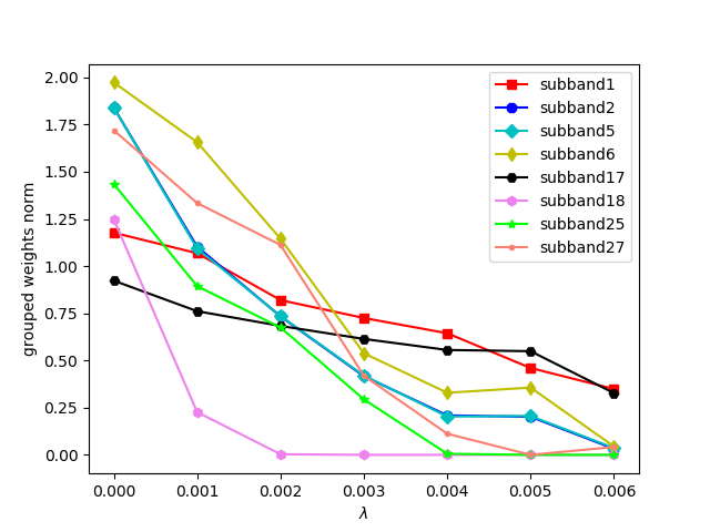
4.5 Grouped Weights Decay
To show the functionality of the group sparsity regularization coefficient , we plot the norms of the grouped weights in the first convolutional layer of our DNN as a function of the group sparsity regularization coefficient for some of the selected wavelet sub-bands (see Figure 5). Increasing the group sparsity penalty coefficient will push the grouped weight norms toward zero as expected.
4.6 Performance of the Deep Morph Detector
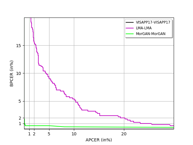
Once we found the top 20 discriminative wavelet sub-bands, we stacked the selected 20 wavelet sub-bands as data samples, and we retrained our modified Inception-ResNet-v1. It should be pointed out that the number of channels is reduced to 20. In the first scenario, we train the DNN using the 20-stacked wavelet sub-bands of each individual dataset, and the performance of the our morph detector is reported using the evaluation metrics introduced in Section 4.4. Table 1 delineates the performance of our deep morph detector when evaluated on our three datasets. Moreover, the corresponding DET curves are shown in Figure 6.a.
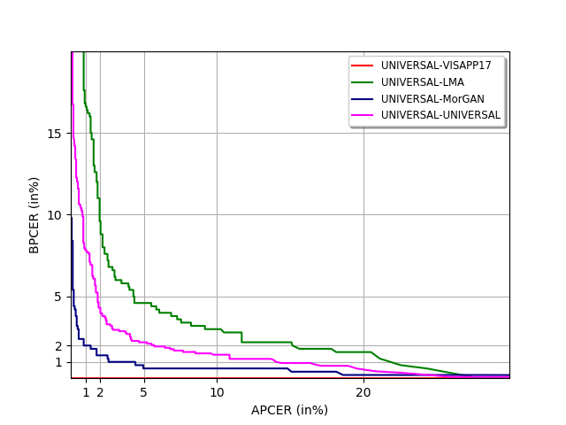
In the second scenario, we trained our DNN detector using the training portion of the universal dataset, and the performance of the deep morph detector is reported using the test set of the universal dataset, as well as the test sets of individual datasets. Table 2 summarizes the evaluation of our morph detector when trained on the universal dataset, and the pertinent DET curves are plotted in Figure 6.b.
Please note that in Table 1 and Table 2, RGB+DNN represents our baseline when the Inception-ResNet-v1 is trained on the original RGB images, and 48-sub-band data indicates the data samples that consist of 48 wavelet sub-bands without utilizing the structured group sparsity. Our results mentioned in Table 1 and Table 2 prove the effectiveness of feature selection scheme for detecting morphed samples. In particular, the morphed samples in the VISAPP17 and MorGAN datasets are detected precisely compared with the LMA dataset. Please note that the performance of our RGB+DNN baseline, which is trained on the Inception-ResNet-v1, is on par with the performance of other DNNs. In particular, regarding the state-of-the-art results, in [11] the morph detection results on the LMA dataset is as follows: D-EER: 0.00, BPCER@APCER=10%: 0.00 , BPCER@APCER=20%: 0.00. Also, their results on the MorGAN dataset is as follows: D-EER: 34.00, BPCER@APCER=10%: 67.00, BPCER@APCER=20%: 78.00. Comparing the state-of-the-art results with ours reveals that our method outperforms on the MorGAN dataset considerably and perform close to this baseline on the LMA dataset.
5 VISUALIZING THE FUNCTIONALITY OF THE DEEP MORPH DETECTOR
In this section, we adopt a few visualization techniques to explain the underlying mechanism of our morph detector. First, we utilize the t-distributed Stochastic Neighbor Embedding (t-SNE) [44] visualization technique to explain the classification performance improvement due to the imposed structured sparsity. Second, we utilize the Gradient-weighted Class Activation Mapping (Grad-CAM) [39] to show the most attended spatial regions in the input images when our trained classifier labels an input image as a bona fide or morphed image.
5.1 Visualizing the Functionality of Structured Group Sparsity
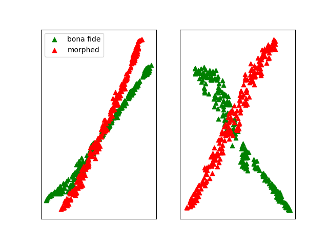
To display the efficacy of our feature selection scheme, which is selecting the most discriminative sub-bands, the t-SNE visualization technique is employed as a representative medium which preserves the local structure of samples when visualizing high dimensional data samples in a low dimensional space. We randomly select 200 bona fide, and 200 morphed samples from the MorGAN dataset for the following two cases. In the first case, we extract the DNN embedding features for the original 48-sub-band data samples for the 200 bona fide and 200 morphed sample. Please note that the employed DNN for feature extraction was already trained on the 48-sub-band data. As the second case, we find the deep features using a DNN trained on the 20-sub-band data for the same 200 bona fide and 200 morphed samples. The point here is that we use the same data samples for both cases, but with different number of wavelet sub-bands. These two subsets of data points are plotted using t-SNE as shown in Figure 7, and we see that 20-sub-band data, in the right column, are more separable compared to the 48-sub-band data in the left column, which substantiates the effectiveness of our feature selection algorithm.
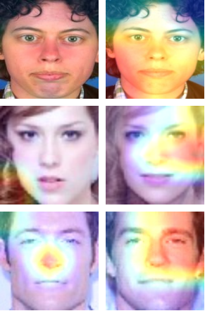
5.2 Grad-CAM Visualization
Understanding the key spatial areas in an input image, in terms of detection or classification, has been a long-standing topic of interest in the vision community. It is worth mentioning that our DNN is a non-attention-based architecture, and we do not use any attention mechanism in our DNN. In this section we adopt another useful visualization technique to observe which regions in the input images are paid more attention to from the DNN perspective in time of inference. In other words, we want to see which pixels are considered discriminative given our morph classification task. To explain the functionality of our trained DNN, we employ the Grad-CAM, which represents the gradient-weighted class activation maps. In this visualization method, the gradient of a class-specific logit is obtained with respect to all spatial locations in a given feature map of the last convolutional layer in the DNN under scrutiny. The calculated gradients are averaged-pooled globally for each feature map, and these coefficients are used for a weighted average of the feature maps along with a final ReLU activation function to produce the class specific Grad-CAM. In accordance with the notation used in [39], the importance of the weights incorporating the pixels in the feature map of the last convolutional layer is as follows:
| (3) |
where represents the total number of spatial locations in the feature map , delineates the score or logit for the class , and denotes the activation or feature map. Consequently, the Grad-CAM produced for class with respect to the final convolutional layer in the DNN is as follows:
| (4) |
To produce the class-specific Grad-CAM for a bona fide image and its corresponding morphed image, we choose the last convolutional layer in our modified Inception-ResNet-v1, which has 1792 feature maps with spatial size of . Based on Figure 8, the right images, that are morphed faces have substantially more attended regions compared to the left images, which are the bona fide samples.
6 CONCLUSION
In this paper, we employed structured group sparsity to force a DNN into finding the most discriminative subset of wavelet sub-bands, that are the wavelet sub-bands. To isolate the discriminating artifacts in the spatial-frequency feature domain, we adapted our framework into the wavelet domain. As far as learning the parameters of our DNN is concerned, the cost function of the DNN is constrained to meet the group Lasso condition, which is imposed on the grouped weights of the first convolutional layer. Our adjusted cost function results in finding the top 20 discriminative wavelet sub-bands, further enabling accurate morph detection with respect to our datasets. The D-EER, APCER5, and APCER10 rates obtained using our trained network with the optimal number of sub-bands substantiate the effectiveness of our framework. In particular, the morphed samples in the VISAPP17, and MorGAN datasets are detected accurately compared to the LMA dataset. In addition, to make the effectiveness of our morph detector transparent, we utilized two visualization techniques to explain the functionality of the proposed single image morph detector.
References
- [1] Rameen Abdal, Yipeng Qin, and Peter Wonka. Image2stylegan: How to embed images into the stylegan latent space? In Proceedings of the IEEE/CVF International Conference on Computer Vision, pages 4432–4441, 2019.
- [2] Poorya Aghdaie, Baaria Chaudhary, Sobhan Soleymani, Jeremy Dawson, and Nasser M Nasrabadi. Attention aware wavelet-based detection of morphed face images. In 2021 IEEE International Joint Conference on Biometrics (IJCB), pages 1–8. IEEE, 2021.
- [3] Poorya Aghdaie, Baaria Chaudhary, Sobhan Soleymani, Jeremy Dawson, and Nasser M Nasrabadi. Detection of morphed face images using discriminative wavelet sub-bands. arXiv preprint arXiv:2106.08565, 2021.
- [4] Stephanie Autherith and Cecilia Pasquini. Detecting morphing attacks through face geometry features. Journal of Imaging, 6(11):115, 2020.
- [5] Kunlun Bai. A comprehensive introduction to different types of convolutions in deep learning. https://towardsdatascience.com/a-comprehensive-introduction-to-different-types-of-convolutions-in-deep-learning-669281e58215, Feb. 2019.
- [6] Herbert Bay, Tinne Tuytelaars, and Luc Van Gool. Surf: Speeded up robust features. In European conference on computer vision, pages 404–417. Springer, 2006.
- [7] Yoshua Bengio, Aaron Courville, and Pascal Vincent. Representation learning: A review and new perspectives. IEEE transactions on pattern analysis and machine intelligence, 35(8):1798–1828, 2013.
- [8] Zander Blasingame and Chen Liu. Leveraging adversarial learning for the detection of morphing attacks. In 2021 IEEE International Joint Conference on Biometrics (IJCB), pages 1–8. IEEE, 2021.
- [9] Naser Damer, Alexandra Moseguí Saladié, Andreas Braun, and Arjan Kuijper. Morgan: Recognition vulnerability and attack detectability of face morphing attacks created by generative adversarial network. In 2018 IEEE 9th International Conference on Biometrics Theory, Applications and Systems (BTAS), pages 1–10. IEEE, 2018.
- [10] Hao Dang, Feng Liu, Joel Stehouwer, Xiaoming Liu, and Anil K Jain. On the detection of digital face manipulation. In Proceedings of the IEEE/CVF Conference on Computer Vision and Pattern recognition, pages 5781–5790, 2020.
- [11] Luca Debiasi, Naser Damer, Alexandra Moseguí Saladié, Christian Rathgeb, Ulrich Scherhag, Christoph Busch, Florian Kirchbuchner, and Andreas Uhl. On the detection of gan-based face morphs using established morph detectors. In International Conference on Image Analysis and Processing, pages 345–356. Springer, 2019.
- [12] Matteo Ferrara, Annalisa Franco, and Davide Maltoni. The magic passport. In IEEE International Joint Conference on Biometrics, pages 1–7. IEEE, 2014.
- [13] Matteo Ferrara, Annalisa Franco, and Davide Maltoni. Face demorphing. IEEE Transactions on Information Forensics and Security, 13(4):1008–1017, 2017.
- [14] Matteo Ferrara, Annalisa Franco, and Davide Maltoni. Face morphing detection in the presence of printing/scanning and heterogeneous image sources. arXiv preprint arXiv:1901.08811, 2019.
- [15] Jie Gui, Zhenan Sun, Shuiwang Ji, Dacheng Tao, and Tieniu Tan. Feature selection based on structured sparsity: A comprehensive study. IEEE transactions on neural networks and learning systems, 28(7):1490–1507, 2016.
- [16] Tao Hu, Honggang Qi, Qingming Huang, and Yan Lu. See better before looking closer: Weakly supervised data augmentation network for fine-grained visual classification. arXiv preprint arXiv:1901.09891, 2019.
- [17] Juho Kannala and Esa Rahtu. Bsif: Binarized statistical image features. In Proceedings of the 21st international conference on pattern recognition (ICPR2012), pages 1363–1366. IEEE, 2012.
- [18] Lingzhi Li, Jianmin Bao, Hao Yang, Dong Chen, and Fang Wen. Advancing high fidelity identity swapping for forgery detection. In Proceedings of the IEEE/CVF Conference on Computer Vision and Pattern Recognition, pages 5074–5083, 2020.
- [19] Lingzhi Li, Jianmin Bao, Ting Zhang, Hao Yang, Dong Chen, Fang Wen, and Baining Guo. Face x-ray for more general face forgery detection. In Proceedings of the IEEE/CVF Conference on Computer Vision and Pattern Recognition, pages 5001–5010, 2020.
- [20] Ziwei Liu, Ping Luo, Xiaogang Wang, and Xiaoou Tang. Deep learning face attributes in the wild. In Proceedings of International Conference on Computer Vision (ICCV), December 2015.
- [21] David G Lowe. Object recognition from local scale-invariant features. In Proceedings of the seventh IEEE international conference on computer vision, volume 2, pages 1150–1157. IEEE, 1999.
- [22] Yi Lu, Ke Xu, Tanfeng Sun, Kaiyue Qi, and Lihong Yao. Face morphing detection with convolutional neural network based on multi-features. In Proceedings of the 2020 International Conference on Aviation Safety and Information Technology, pages 611–616, 2020.
- [23] Andrey Makrushin, Tom Neubert, and Jana Dittmann. Automatic generation and detection of visually faultless facial morphs. In VISIGRAPP (6: VISAPP), pages 39–50, 2017.
- [24] Tom Neubert, Christian Kraetzer, and Jana Dittmann. A face morphing detection concept with a frequency and a spatial domain feature space for images on emrtd. In Proceedings of the ACM Workshop on Information Hiding and Multimedia Security, pages 95–100, 2019.
- [25] Sophie J Nightingale, Shruti Agarwal, and Hany Farid. Perceptual and computational detection of face morphing. Journal of Vision, 21(3):4–4, 2021.
- [26] Timo Ojala, Matti Pietikainen, and David Harwood. Performance evaluation of texture measures with classification based on kullback discrimination of distributions. In Proceedings of 12th International Conference on Pattern Recognition, volume 1, pages 582–585. IEEE, 1994.
- [27] Yuyang Qian, Guojun Yin, Lu Sheng, Zixuan Chen, and Jing Shao. Thinking in frequency: Face forgery detection by mining frequency-aware clues. In European Conference on Computer Vision, pages 86–103. Springer, 2020.
- [28] R. Raghavendra, K. Raja, S. Venkatesh, and C. Busch. Face morphing versus face averaging: Vulnerability and detection. In 2017 IEEE International Joint Conference on Biometrics (IJCB), pages 555–563, 2017.
- [29] R. Raghavendra, K. B. Raja, and C. Busch. Detecting morphed face images. In 2016 IEEE 8th International Conference on Biometrics Theory, Applications and Systems (BTAS), pages 1–7, 2016.
- [30] Kiran Raja, Sushma Venkatesh, RB Christoph Busch, et al. Transferable deep-cnn features for detecting digital and print-scanned morphed face images. In Proceedings of the IEEE Conference on Computer Vision and Pattern Recognition Workshops, pages 10–18, 2017.
- [31] Ulrich Scherhag, Luca Debiasi, Christian Rathgeb, Christoph Busch, and Andreas Uhl. Detection of face morphing attacks based on prnu analysis. IEEE Transactions on Biometrics, Behavior, and Identity Science, 1(4):302–317, 2019.
- [32] Ulrich Scherhag, Jonas Kunze, Christian Rathgeb, and Christoph Busch. Face morph detection for unknown morphing algorithms and image sources: a multi-scale block local binary pattern fusion approach. IET Biometrics, 9(6):278–289, 2020.
- [33] Ulrich Scherhag, Ramachandra Raghavendra, Kiran B Raja, Marta Gomez-Barrero, Christian Rathgeb, and Christoph Busch. On the vulnerability of face recognition systems towards morphed face attacks. In 2017 5th International Workshop on Biometrics and Forensics (IWBF), pages 1–6. IEEE, 2017.
- [34] Ulrich Scherhag, Christian Rathgeb, and Christoph Busch. Morph deterction from single face image: A multi-algorithm fusion approach. In Proceedings of the 2018 2nd International Conference on Biometric Engineering and Applications, pages 6–12, 2018.
- [35] Ulrich Scherhag, Christian Rathgeb, and Christoph Busch. Performance variation of morphed face image detection algorithms across different datasets. In 2018 International Workshop on Biometrics and Forensics (IWBF), pages 1–6. IEEE, 2018.
- [36] Ulrich Scherhag, Christian Rathgeb, Johannes Merkle, Ralph Breithaupt, and Christoph Busch. Face recognition systems under morphing attacks: A survey. IEEE Access, 7:23012–23026, 2019.
- [37] Clemens Seibold, Wojciech Samek, Anna Hilsmann, and Peter Eisert. Detection of face morphing attacks by deep learning. In International Workshop on Digital Watermarking, pages 107–120. Springer, 2017.
- [38] Clemens Seibold, Wojciech Samek, Anna Hilsmann, and Peter Eisert. Accurate and robust neural networks for security related applications exampled by face morphing attacks. arXiv preprint arXiv:1806.04265, 2018.
- [39] Ramprasaath R Selvaraju, Michael Cogswell, Abhishek Das, Ramakrishna Vedantam, Devi Parikh, and Dhruv Batra. Grad-cam: Visual explanations from deep networks via gradient-based localization. In Proceedings of the IEEE international conference on computer vision, pages 618–626, 2017.
- [40] Jag Mohan Singh, Raghavendra Ramachandra, Kiran B Raja, and Christoph Busch. Robust morph-detection at automated border control gate using deep decomposed 3d shape & diffuse reflectance. In 2019 15th International Conference on Signal-Image Technology & Internet-Based Systems (SITIS), pages 106–112. IEEE, 2019.
- [41] Luuk Spreeuwers, Maikel Schils, and Raymond Veldhuis. Towards robust evaluation of face morphing detection. In 2018 26th European Signal Processing Conference (EUSIPCO), pages 1027–1031. IEEE, 2018.
- [42] Christian Szegedy, Sergey Ioffe, Vincent Vanhoucke, and Alexander A Alemi. Inception-v4, inception-resnet and the impact of residual connections on learning. In Thirty-first AAAI conference on artificial intelligence, 2017.
- [43] Robert Tibshirani. Regression shrinkage and selection via the lasso. Journal of the Royal Statistical Society: Series B (Methodological), 58(1):267–288, 1996.
- [44] Laurens Van der Maaten and Geoffrey Hinton. Visualizing data using t-sne. Journal of machine learning research, 9(11), 2008.
- [45] Sushma Venkatesh, Raghavendra Ramachandra, Kiran Raja, and Christoph Busch. Face morphing attack generation & detection: A comprehensive survey. IEEE Transactions on Technology and Society, 2021.
- [46] Sushma Venkatesh, Raghavendra Ramachandra, Kiran Raja, Luuk Spreeuwers, Raymond Veldhuis, and Christoph Busch. Detecting morphed face attacks using residual noise from deep multi-scale context aggregation network. In The IEEE Winter Conference on Applications of Computer Vision, pages 280–289, 2020.
- [47] Wei Wen, Chunpeng Wu, Yandan Wang, Yiran Chen, and Hai Li. Learning structured sparsity in deep neural networks. In Advances in neural information processing systems, pages 2074–2082, 2016.
- [48] Shuo Xiang, Xiaoshen Tong, and Jieping Ye. Efficient sparse group feature selection via nonconvex optimization. In International Conference on Machine Learning, pages 284–292. PMLR, 2013.
- [49] Luyu Yang, Chenqiang Gao, Deyu Meng, and Lu Jiang. A novel group-sparsity-optimization-based feature selection model for complex interaction recognition. In Asian Conference on Computer Vision, pages 508–521. Springer, 2014.
- [50] Ming Yuan and Yi Lin. Model selection and estimation in regression with grouped variables. Journal of the Royal Statistical Society: Series B (Statistical Methodology), 68(1):49–67, 2006.
- [51] Le-Bing Zhang, Fei Peng, and Min Long. Face morphing detection using fourier spectrum of sensor pattern noise. In 2018 IEEE International Conference on Multimedia and Expo (ICME), pages 1–6. IEEE, 2018.
- [52] Shaoting Zhang, Junzhou Huang, Hongsheng Li, and Dimitris N Metaxas. Automatic image annotation and retrieval using group sparsity. IEEE transactions on systems, man, and cybernetics, Part B (Cybernetics), 42(3):838–849, 2012.
- [53] Hanqing Zhao, Wenbo Zhou, Dongdong Chen, Tianyi Wei, Weiming Zhang, and Nenghai Yu. Multi-attentional deepfake detection. In Proceedings of the IEEE/CVF Conference on Computer Vision and Pattern Recognition, pages 2185–2194, 2021.