Detection of collinear high energetic di-photon signatures with Micromegas Detectors

Abstract

The search for weakly interacting, light particles that couple to photons received significant attention in recent years. When those particles are produced at high energies, they lead to two, nearly collinear photons after their decay and hence can be detected by an electromagnetic calorimeter system. The typical dominant background in searches for those high energetic weakly particles are single, high energetic photons, which leave similar signatures in a standard calorimeter system. One promising approach to separate signal from background events is to employ a dedicated pre-shower detector in front of the calorimeter that can distinguish one- and two-photon signatures. In this work we present a conceptual design of such detector which is able to separate one from two collinear photon signatures with efficiencies between $20\text{\,}\mathrm{\char 37\relax}$ to $80\text{\,}\mathrm{\char 37\relax}$ for two photons separated by $100\text{\,}\mathrm{\SIUnitSymbolMicro m}$ to $2000\text{\,}\mathrm{\SIUnitSymbolMicro m}$, respectively, with energies above $300\text{\,}\mathrm{GeV}$ and a background rejection of more than $90\text{\,}\mathrm{\char 37\relax}$. Our pre-shower detector design has an active surface area of $10\text{\times}10\text{\,}{\mathrm{cm}}^{2}$, a depth of $230\text{\,}\mathrm{mm}$ and is based on Micromegas detectors, thus offering a cost effective solution.

1 Introduction

Axions and other very light axion-like particles (ALPs) [1, 2] appear in many extensions of the Standard Model and are well motivated theoretically: ALPs can solve the well-known strong CP problem [3, 4], act as a dark matter candidate [5] and could also explain the famous muon $(g_{\mu}-2)$ discrepancy [6]. The experimental effort to search for ALPs as dark matter candidates is ongoing and has been considerably intensified in recent years, leading to the proposal and construction of a wide range of dedicated experiments. ALPs with masses in the $\mathrm{MeV}$ regime and above are typically searched for in collider experiments, such as the ForwArd Search ExpeRiment (FASER) [7, 8], which was installed in the LHC in March 2021 and is situated $480\text{\,}\mathrm{m}$ along the line-of-sight of the proton collisions in front of the ATLAS interaction point at the LHC. ALPs are produced in collider experiments with typical momenta that are much larger than their mass, hence the generic experimental signatures are two highly collinear photons. While standard calorimeters can measure the total energy of those photons, they have no means to distinguish their electromagnetic showers if the distance between them is smaller than the cell-size of the calorimeter system.

In this paper, we present a conceptual pre-shower detector design that is able to separate high energetic one-photon events from collinear two-photon events. This separation is achieved by alternating layers of tungsten, that act as passive material triggering photon conversions and subsequent electromagnetic showers; and Micromegas detectors, for the reconstruction of charged particles. In total three layers of tungsten and three Micromegas detectors with an active area of $10\text{\times}10\text{\,}{\mathrm{cm}}^{2}$ and a two-dimensional readout are used. A simulation based on Geant4 was developed to evaluate the expected performance of the preshower detector, using deep neural networks for the event classification. The simulation was validated by test beam measurements at the MAMI (MAinz MIcrotron) accelerator. The optimisation of the detector layer as well as the prototype detector which was used during the test beam measurements is discussed in Section 2. The simulation as well as its validation is summarized in Section 3, followed by a discussion of the photon identification algorithm (Section 4) and the results (Section 5).

2 Detector Layout and Optimization

The schematic design of the pre-shower detector is shown in Figure 1. The number of passive tungsten layers as well as the number of active Micromegas detectors was fixed in our design approach as our total pre-shower detector should not exceed a potential minimal depth of $\approx$20 cm, however, the thickness of the tungsten layers was subject to optimization.

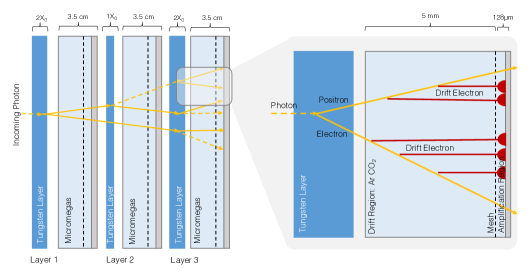
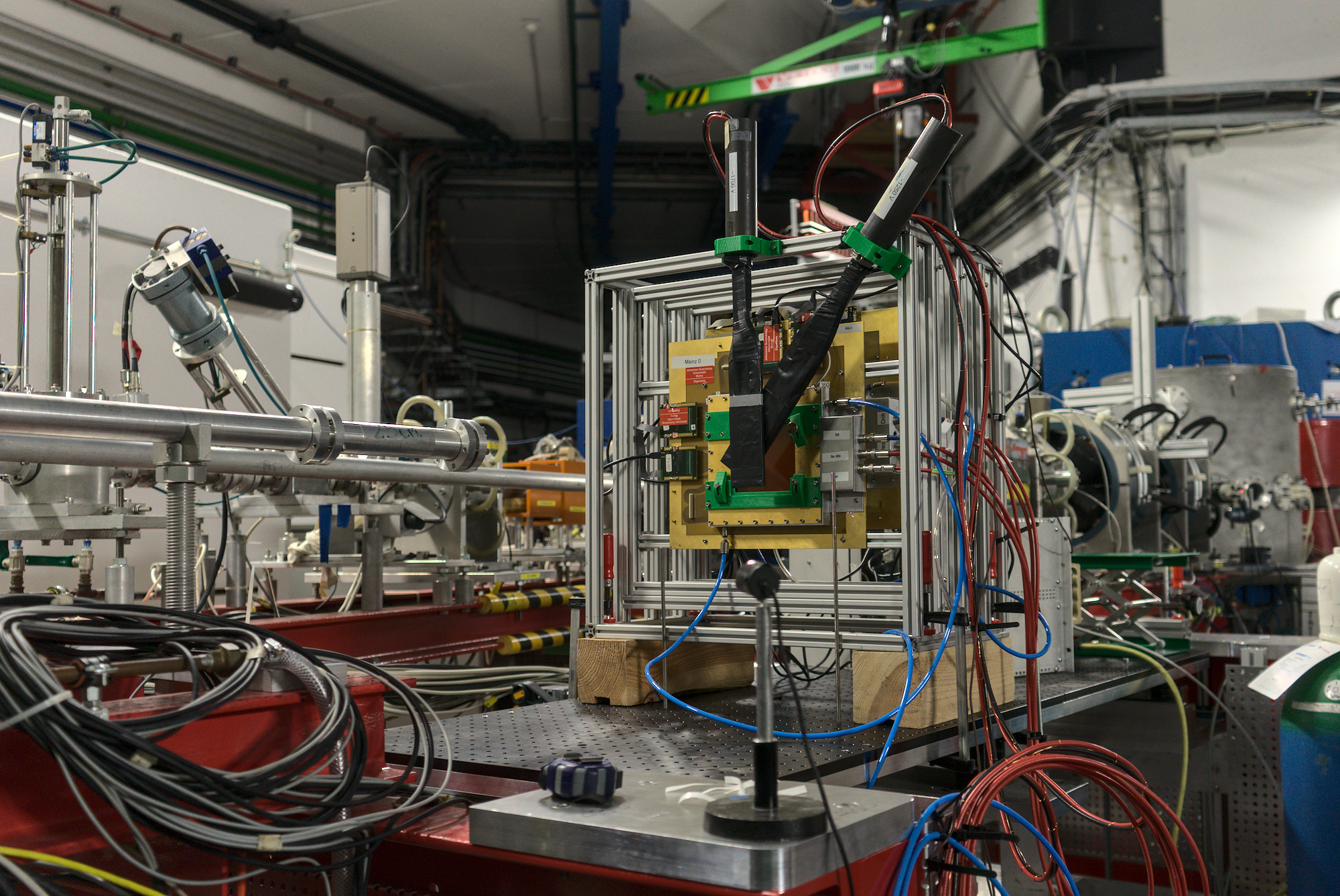
Figure 1: Schematic layout of the detector setup (left) as well as picture of the prototype in the test beam setup (right).

We propose to use standard Micromegas detectors with a two-dimensional readout, which have been originally designed by the MAMMA collaboration [9] and are described in detail in [10]. They have an active area of $10\text{\times}10\text{\,}\mathrm{cm}$ and a depth of $3.5\text{\,}\mathrm{cm}$ and have proven to operate with a high reliability, a very good spatial resolution of $<200\text{\,}\mathrm{\SIUnitSymbolMicro m}$ and also, they are not subject to dead-times from sparks. The drift-region, filled with a gas mixture of $93\text{\,}\mathrm{\char 37\relax}$ Argon and $7\text{\,}\mathrm{\char 37\relax}$ CO₂, has a depth of $5\text{\,}\mathrm{mm}$, while the amplification region has a depth of $128\text{\,}\mathrm{\SIUnitSymbolMicro m}$. The readout electrode of each detector comprises 360 copper readout strips in two separate, orthogonal layers with a strip pitch of $250\text{\,}\mathrm{\SIUnitSymbolMicro m}$, allowing to measure two-dimensional spatial information. The readout strips of the upper layer (defined as $y$-layer) are printed directly on top of the PCB and are covered by the resistive strips with a resistivity of $20\text{\,}\mathrm{M\SIUnitSymbolOhm}\text{\,}{\mathrm{cm}}^{-1}$. The lower layer (defined as $x$-layer) is separated from the upper layer by $70\text{\,}\mathrm{\SIUnitSymbolMicro m}$ of FR4, i.e. the same material used as isolating material in the PCB. The readout strips of the $x$-layer have a width of $200\text{\,}\mathrm{\SIUnitSymbolMicro m}$ and are placed parallel to the resistive strips, while the strips in the $y$-layer have a width of $80\text{\,}\mathrm{\SIUnitSymbolMicro m}$ and are perpendicularly placed with respect to the resistive strips. The larger width of the $x$-layer readout strips compensates for their weaker capacitive coupling. The woven mesh is made of stainless steel with a density of $157\text{\,}\mathrm{l}\mathrm{i}\mathrm{n}\mathrm{e}\mathrm{s}\mathrm{/}\mathrm{c}\mathrm{m}$ and a diameter of $18\text{\,}\mathrm{\SIUnitSymbolMicro m}$. It is mounted on support pillars of $0.4\text{\,}\mathrm{mm}$ diameter and covers an area of $10\text{\times}10\text{\,}\mathrm{cm}$ which defines the active area of the detector. The support pillars are placed along a regular matrix with $2.5\text{\,}\mathrm{mm}$ spacing in both directions.

The data acquisition is based on the RD51 Scalable Readout System (SRS) [11, 12]. The signal processing of the detector is based on the Analog Pipeline Voltage chip with $0.25\text{\,}\mathrm{\SIUnitSymbolMicro m}$ CMOS technology (APV25) [13] where the analog signal data is transmitted via HDMI cables to SRS electronics. The SRS electronics process the analog signal which is then further analyzed. It should be noted that the height of the recorded readout signal is related to the charge induced on the readout strip. The photon identification algorithms are based on the measured integrated charge in each strip of both layers in all three Micromegas detectors, since the measured charge is correlated with the number of created charged particles in the drift region of the detector. No timing information was used.

The figure of merit for the optimization of the system was the correct identification of two photon events with a separation of $200\text{\,}\mathrm{\SIUnitSymbolMicro m}2000\text{\,}\mathrm{\SIUnitSymbolMicro m}$ and energies of $100\text{\,}\mathrm{GeV}3500\text{\,}\mathrm{GeV}$ and one-photon events with energies of $200\text{\,}\mathrm{GeV}7000\text{\,}\mathrm{GeV}$. Several layouts have been tested, using the simulation and classification algorithms described in more detail in Sections 3 and 4. Optimal results have been achieved for $2\text{\,}\mathrm{$X_{0}$}$ of tungsten in front of the first and the last active layer and $1\text{\,}\mathrm{$X_{0}$}$ in front of the second active layer, with a separation of $7\text{\,}\mathrm{cm}$ between the active planes.

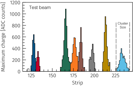
Figure 2: Single event in the Y-layer of the middle detector from the test beam (left) and from simulation (right). The different colors indicate the selected clusters.

3 Prototype Detector Simulation and Validation with test beam Measurements

Since it is highly challenging to organize test beam measurement campaigns which would allow to measure directly the pre-shower detector performance for the separation of collinear photon signatures at energies above several hundred $\mathrm{GeV}$, an alternative approach has been taken: one specific detector layout was setup and studied in test beam measurements. These measurements are then used to validate the Geant4 based simulation, which is used in a second step to estimate the detector performance for the separation of collinear photon signatures.

Incident electrons and photons may create an electromagnetic shower via Bremsstrahlung and pair-production in the tungsten layers, leading to electron positron pairs which enter the drift-region of the Micromegas detector, where they will interact with and ionize gas atoms. The resulting ionization electrons will drift to the amplification region and hence, induce a signal at the corresponding readout strips. Typically, signals due to one incident primary particle, i.e. electron or photon, will induce electric signal in neighbouring readout strips, leading to clusters. To find clusters in a first step, peaks are searched in the maximum charge distribution. The extent of the cluster is determined iterating the neighbouring strips of each peak in both directions until either more than two strips without charge are found or the charge is increasing. This allows to separate close-by clusters as long as they are not fully overlapping. The size of those cluster is then defined by the number of strips hit. Examples of the recorded charge distribution per readout strip for one electron event that produced a shower in the tungsten layers are shown in Figure 2 for the test beam measurement as well as the simulation, where several clusters can be clearly identified.

The recorded signal height as well as its time evolvement within one cluster depends on one hand, on the number of corresponding drift electrons and on the other hand, on the applied amplification voltage. The position of one cluster is defined as the weighted mean of all associated readout-strips with their measured signal. For the photon identification algorithm the maximum charge from each strip is taken and fed as an input to the neural network. It is therefore important that the number of clusters as well as their charge distribution is correctly described in the simulation.

The test beam setup of the pre-shower detector consists also of three active Micromegas planes that are interleaved by three layers of tungsten with a variable thickness of $1\text{\,}\mathrm{mm}$ to $6\text{\,}\mathrm{mm}$ (Figure 1). The distance between the passive tungsten and active Micromegas layers was $4\text{\,}\mathrm{mm}$ with $75\text{\,}\mathrm{mm}$ distance between the Micromegas layers to allow accessing the tungsten layers, yielding a total length of the prototype detector of $230\text{\,}\mathrm{mm}$. Different thicknesses of the tungsten layers have been chosen during the test beam measurements in order to validate the detector simulation over a larger parameter space. The test beam measurements have been conducted in 2020 at the MAMI accelerator facility at the Johannes Gutenberg University Mainz. MAMI provides a quasi-continuous electron beam with energy up to $1.5\text{\,}\mathrm{GeV}$. A beam energy of $855.1\text{\,}\mathrm{MeV}$ was used for the measurements presented in this paper. Clean signals have been recorded by applying drift and amplification voltages of $V_{D}=$300\text{\,}\mathrm{V}200\text{\,}\mathrm{V}225\text{\,}\mathrm{V}$$ and $V_{A}=$560\text{\,}\mathrm{V}565\text{\,}\mathrm{V}570\text{\,}\mathrm{V}$$ respectively for the three Micromegas detectors. The beam axis was chosen to be perpendicular to the readout-panels.

The test beam setup was then implemented also in the Geant4 simulation framework. The interaction of the incident electrons with the detector material and the propagation of the particles of the resulting electromagnetic shower through the detector, in particular the energy deposits within the drift volume of the Micromegas detectors, are simulated directly by Geant4. The position of each energy deposit is stored. Then the charge deposits are added to the strips based on event shapes extracted from data. The amplitude is determined by multiplying the deposited energy from Geant4 with a fixed gain factor for each layer. This allowed getting a reasonable description of the maximum charges for a first study without requiring a detailed simulation of the gas transport, amplification and digitization. Once the simulation has been implemented, the detector response of $100\,000$ events of incoming electrons with a energy of $855.1\text{\,}\mathrm{MeV}$ has been simulated.

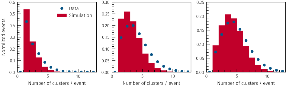
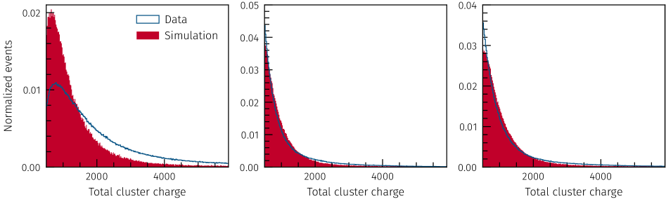
Figure 3: Comparison of the number of reconstructed clusters (top) and the total charge per cluster (bottom) in the $y$-layers of all detectors in simulation (bars) and test beam measurements (points/line).

In a second step, the cluster-finding algorithm has been applied to the test beam data and the simulation. The electronic response parameters have been tuned such that they describe the observed cluster properties, in particular the cluster-size as well as the signal height. It has been tested for all available setups of the prototype detector used during the test beam campaign. Figure 3 shows the number of reconstructed clusters as well as the total charge per cluster in all detector layers in simulation and measurement for the setup with $1\text{\,}\mathrm{$X_{0}$}$ in front of the first two layers and $2\text{\,}\mathrm{$X_{0}$}$ in front of the last layer. The mean of the number of clusters between data and simulation agrees at a $10\text{\,}\mathrm{\char 37\relax}$ level, however, systematically more clusters are reconstructed in data than simulation. This can be explained by dead channels not being explicitly modelled as well as by differences in the detector gain. Similarly, the total cluster charge is larger in data than in simulation. The largest deviation is found in the first detector layer which can be explained by sub-optimal bias voltage settings during the test beam. The effect of this disagreement on the final photon identification algorithms has been tested by scaling the simulated charge deposits.

Once the simulation was tuned and validated for the electron beam, the same setup was used to simulate single and di-photon events with various event kinematics: events are evenly distributed in the parameter space with the photon energies within $200\text{\,}\mathrm{GeV}7000\text{\,}\mathrm{GeV}$ for single photons and $100\text{\,}\mathrm{GeV}3500\text{\,}\mathrm{GeV}$ for di-photon events. The separation between the two photons is taken to be within $0\text{\,}\mathrm{\SIUnitSymbolMicro m}2000\text{\,}\mathrm{\SIUnitSymbolMicro m}$. In total 6 million single photon and 12 million di-photon events are simulated. The higher number of di-photon events is chosen to compensate for the lower event yield when applying filter criteria on the photon conversion.

4 Di-photon Identification

Single photon events are expected to produce fewer clusters in each layer compared to di-photon events. Moreover, the cluster distribution is expected to be narrower for the former, compared to the latter. For an optimal classification of single- and di-photon events, a deep convolutional neural network based classifier has been used.

For the nominal geometry with $1\text{\,}\mathrm{$X_{0}$}$ worth of absorber material in front of the first detector, $18.7\text{\,}\mathrm{\char 37\relax}$ of the photons produce less than $25$ hits. For the alternative geometry with $2\text{\,}\mathrm{$X_{0}$}$ of absorber, this number drops to only $10\text{\,}\mathrm{\char 37\relax}$ of photons producing less than $25$ hits due to the photon shower being initiated earlier. To ensure that the training consists mostly of events where the photons converted at least $25$ hits per photon are required across the three detectors. The training is performed using Keras [14] with Tensorflow [15] as the back-end.

The network takes inputs in two stages. First, the charge on each strip (total of 2160 inputs) is fed into one dimensional convolutions. The output of the convolution is reduced to a single dimension by a flatten layer. Afterwards, the total energy of the event is inserted as an additional input and passed into three dense layers. Here, the total event energy is smeared to reflect the resolution of a typical electromagnetic calorimeter. Finally, a layer with only a single output neuron is used. The activation function is a rectified linear unit for all layers except for the output layer which uses a sigmoid as the activation to ensure an output between $0$ and $1$. The labels are chosen such that the output is $0$ for single photon events and $1$ for di-photon events.

The network architecture has been optimized by minimizing the loss defined by binary cross-entropy. The parameters for the convolution layers, number of fully connected layers and number of neurons were determined by running a hyper-parameter scan where the architecture with the highest validation accuracy was selected. The parameters of the full network architecture are summarized in Table 1.

Layer type	Neurons	Kernel size / Filters	Parameters
Input (charges)
1D Conv.		$14$ / $20$	$6800$
Max. pooling
Flatten
Input (energy)
Concatenate
Dense	$40$		$576\,080$
Dense	$20$		$820$
Dense	$10$		$210$
Output	$1$		$11$
Total			$583\,921$

Table 1: Architecture of the neural network used for discriminating between single and di-photon events. Between each two layers, a dropout layer with a dropout rate of $0.1$ is present. ReLu is used as the activation function for all layers except the output which uses a sigmoid function.

5 Results

The expected performance of our preshower detector and di-photon reconstruction algorithm has been tested by using simulated events, which have not been used during the training of the network. First, we discuss the expected performance for several chosen single- and di-photon kinematics, followed by a discussion of the performance for ALP decays, where a convolution of several effects plays a role.

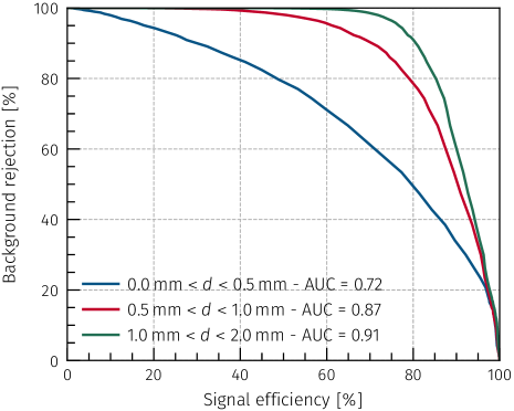
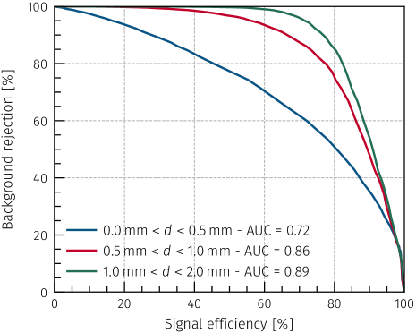
Figure 4: ROC curves of di-photon events evaluated for different photon distance ranges for photons with equal energies of $500\text{\,}\mathrm{GeV}$ (left) and asymmetric energies of $800\text{\,}\mathrm{GeV}$ and $200\text{\,}\mathrm{GeV}$ (right); and $1\text{\,}\mathrm{TeV}$ for single photon backgrounds. AUC stands for area under the curve.

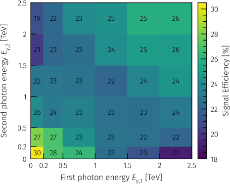
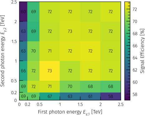
Figure 5: Signal efficiency for di-photon events evaluated in dependence of the two photons energy in multiple bins for di-photon events with a separation of $<300\text{\,}\mathrm{\SIUnitSymbolMicro m}$ (left) and for $$500\text{\,}\mathrm{\SIUnitSymbolMicro m}$<d<$1000\text{\,}\mathrm{\SIUnitSymbolMicro m}$$ (right) at an average background rejection of $90\text{\,}\mathrm{\char 37\relax}$.

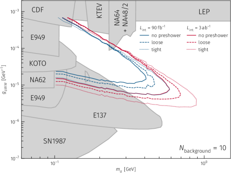
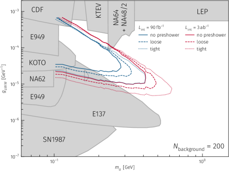
Figure 6: Maximum limits on the $3\sigma$ sensitive region in the ALP mass and coupling plane for integrated luminosities of $90\text{\,}{\mathrm{fb}}^{-1}$ (blue) and $3\text{\,}{\mathrm{ab}}^{-1}$ (red) for the assumption of 10 (left) and 200 (right) background events. Three different scenarios are shown: no preshower (solid), the loose working point with $90\text{\,}\mathrm{\char 37\relax}$ background rejection (dashed) and the thight working point with $99.5\text{\,}\mathrm{\char 37\relax}$ background rejection (dotted). As the expected number of events is only available for a minimum separation of $200\text{\,}\mathrm{\SIUnitSymbolMicro m}$ the reach is only calculated for this fiducial region. Already excluded regions are shown in grey and are taken from [16].

A good measure for the binary classifier is the Receiver Operating Characteristic (ROC) curve, defined by varying the classification-threshold and calculating the corresponding signal efficiency and the background rejection rate. An optimal classifier would yield an integral of the ROC curve of 1, while a pure random classifier for equal signal and background data-sets yields a value of 0.5. Figure 4 shows the ROC curves for two photon signatures with energies of $500\text{\,}\mathrm{GeV}$ and distances between them of $0\text{\,}\mathrm{\SIUnitSymbolMicro m}500\text{\,}\mathrm{\SIUnitSymbolMicro m}$, $500\text{\,}\mathrm{\SIUnitSymbolMicro m}1000\text{\,}\mathrm{\SIUnitSymbolMicro m}$ and $1000\text{\,}\mathrm{\SIUnitSymbolMicro m}2000\text{\,}\mathrm{\SIUnitSymbolMicro m}$ (signal) and single photon events with energies of $1\text{\,}\mathrm{TeV}$ (background). Figure 4 also shows the results for the same samples, however, the energies of the di-photon signals are now not equally shared but $800\text{\,}\mathrm{GeV}$ and $200\text{\,}\mathrm{GeV}$. We observe only minor differences between the symmetric and asymmetric energy split, however, as seen in the area under the curve (AUC) the efficiency for the symmetric case is slightly better. Evaluating the efficiencies with samples where the charge on all strips is scaled by $10\text{\,}\mathrm{\char 37\relax}$ up or down to account for the observed mismodelling in the simulation leads to a relative change of at most $4\text{\,}\mathrm{\char 37\relax}$ in the signal efficiency and $3.5\text{\,}\mathrm{\char 37\relax}$ in the background rejection.

Figure 5 shows the efficiencies for di-photon separations of $d<$300\text{\,}\mathrm{\SIUnitSymbolMicro m}$$ and $$500\text{\,}\mathrm{\SIUnitSymbolMicro m}$<d<$1000\text{\,}\mathrm{\SIUnitSymbolMicro m}$$ for a working point with $90\text{\,}\mathrm{\char 37\relax}$ average background rejection. As expected, it can be seen that the efficiency for small photon separations is lower compared to larger separations. In fact, the signal efficiency ranges from $19\text{\,}\mathrm{\char 37\relax}$ to $79.5\text{\,}\mathrm{\char 37\relax}$ for two photons separated by $100\text{\,}\mathrm{\SIUnitSymbolMicro m}$ to $2000\text{\,}\mathrm{\SIUnitSymbolMicro m}$, respectively, with energies above $100\text{\,}\mathrm{GeV}$, each, at an average background rejection rate of $90\text{\,}\mathrm{\char 37\relax}$ for a single photon with an energy above $200\text{\,}\mathrm{GeV}$.

6 Applications in Axion Search Experiments

As already previously motivated, the developed pre-shower detector could be directly applied in future Axion search experiments, such as FASER. Hence we estimate in the following the expected performance of the detector system for a concrete example. The kinematics of di-photons from ALP decays depend on the axion mass, $m_{a}$, the initial axion momentum as well as the coupling to photons $c_{a\gamma\gamma}$. The smaller the axion mass and the higher the axion momentum, the smaller the expected average distance of the two photons. Moreover, the energy of the two photons can be highly asymmetric depending on the relative orientation of the axion-decay in its restframe to the axion boost direction. A symmetric energy distribution between the two decay photons is therefore only expected if the decay is perpendicular to the axion momentum.

The physics reach for the observation of an axion signal with a confidence level of $3\sigma$ at the FASER experiment for several sencarios has been studied. The expected axion signal events are taken from simulation and are evaluated for 1452 different combinations of the ALP mass $m_{a}$ and coupling $g_{aWW}$ in the range $m_{a}=$0.1\text{\,}\mathrm{GeV}2\text{\,}\mathrm{GeV}$$ and $g_{aWW}=$5\text{\times}{10}^{-7}\text{\,}{\mathrm{GeV}}^{-1}8\text{\times}{10}^{-4}\text{\,}{\mathrm{GeV}}^{-1}$$. The integrated luminosity is fixed to $90\text{\,}{\mathrm{fb}}^{-1}$ reflecting a fraction of LHC-Run 2 and $3\text{\,}{\mathrm{ab}}^{-1}$ reflecting the High-Luminosity LHC. As a detailed simulation of the background is not available at point, the reach is evaluated for the assumptions of 10 or 200 background events for $90\text{\,}{\mathrm{fb}}^{-1}$ and 333 or 6666 background events for $3\text{\,}{\mathrm{ab}}^{-1}$, respectively.

The number of observed events is calculated by convoluting the number of expected events with a given kinematic in dependence of the two photon energies and their distance with the corresponding expected signal efficiencies of our pre-shower detector. The resulting physics yield is summarized in Figure 6 and has been evaluated for two different working points with a background rejection of $90\text{\,}\mathrm{\char 37\relax}$ (loose) and $99.5\text{\,}\mathrm{\char 37\relax}$ (tight), with corresponding average signal efficiencies of approximately $45\text{\,}\mathrm{\char 37\relax}$ and $30\text{\,}\mathrm{\char 37\relax}$. The systematic variation of the measured charge has negligible influence on the physics yield. The tight classification option significantly outperforms the loose option. Moreover it becomes evident that the pre-shower detectors extends the physics reach by a factor of three in axion mass and and a factor of five in the axion coupling strength.

7 Conclusion

A preshower detector based on three active layers of Micromegas detectors was presented, which is able to separate high energetic one-photon from two-photon events. Each of those Micromegas detectors has a depth of $1.5\text{\,}\mathrm{cm}$, is spark-resistant due to a resistive protection layer and allows for a spatial resolution of below $120\text{\,}\mathrm{\SIUnitSymbolMicro m}$, even at very high rates. The measured signals of the active layers are fed to a deep neural network, which acts as binary classifier. The efficiency ranges from $19\text{\,}\mathrm{\char 37\relax}$ to $79.5\text{\,}\mathrm{\char 37\relax}$ for two high energetic photons separated by $100\text{\,}\mathrm{\SIUnitSymbolMicro m}$ to $2000\text{\,}\mathrm{\SIUnitSymbolMicro m}$, respectively with a background rejection rate of $90\text{\,}\mathrm{\char 37\relax}$ for single photons. The efficiency is thereby rising fast with increasing photon distance reaching the plateau at $1000\text{\,}\mathrm{\SIUnitSymbolMicro m}$. The energy dependence is relatively small and the efficiency only drops significantly for one of the photons being less than $200\text{\,}\mathrm{GeV}$. In a second step, we estimated the increase of the sensitivity to the search for axion like particles at the FASER experiment when using the pre-shower detector. It was found that an increase by several factors in axion mass and coupling can be expected. In summary, the developed pre-shower detector design as well as the prototype detector offer a cost effective solution for the event classification of future experiments that aim for the discovery of ALPs in a mass region between $1\text{\,}\mathrm{MeV}$ and $5\text{\,}\mathrm{G}\mathrm{e}\mathrm{V}$ in the di-photon final state.

References

- [1] S. Weinberg “A New Light Boson?” In Phys.Rev.Lett. 40, 1978, pp. 223 DOI: 10.1103/PhysRevLett.40.223
- [2] F. Wilczek “Problem of Strong P and T Invariance in the Presence of Instantons” In Phys.Rev.Lett. 40, 1978, pp. 279 DOI: 10.1103/PhysRevLett.40.279
- [3] R. D. Peccei and H. R. Quinn “CP Conservation in the Presence of pseudoparticles” In Phys.Rev.Lett. 38(25), 1977, pp. 1440 DOI: 10.1103/PhysRevLett.38.1440
- [4] R. D. Peccei and H. R. Quinn “Constraints imposed by CP conservation in the presence of pseudoparticles” In Phys.Rev.D 16, 1977, pp. 1791 DOI: 10.1103/PhysRevD.16.1791
- [5] D. Cadamuro M. Goodsell J. Jaeckel J. RedondoΩP. Arias and A. Ringwald. “WISPy Cold Dark Matter” In JCAP 2012.06, 2012, pp. 013 DOI: 10.1088/1475-7516/2012/06/013
- [6] Martin Bauer, Matthias Neubert and Andrea Thamm “LHC as an Axion Factory: Probing an Axion Explanation for with Exotic Higgs Decays” In Phys. Rev. Lett. 119.3, 2017, pp. 031802 DOI: 10.1103/PhysRevLett.119.031802
- [7] FASER Collaboration “FASER: ForwArd Search ExpeRiment at the LHC”, 2019 arXiv: http://arxiv.org/abs/1901.04468
- [8] FASER Collaboration “FASER’s Physics Reach for Long-Lived Particles” In Physical Review D 99.9, 2019, pp. 095011 DOI: 10.1103/PhysRevD.99.095011
- [9] M. Byszewski and J. Wotschack “Resistive-Strips Micromegas Detectors with Two-Dimensional Readout” In JINST 7, 2012, pp. C02060 DOI: 10.1088/1748-0221/7/02/C02060
- [10] Tai-Hua Lin et al. “Signal Characteristics of a Resistive-Strip Micromegas Detector with an Integrated Two-Dimensional Readout” In Nucl. Instrum. Meth. A 767, 2014, pp. 281–288 DOI: 10.1016/j.nima.2014.09.002
- [11] S Martoiu, H Muller, A Tarazona and J Toledo “Development of the Scalable Readout System for Micro-Pattern Gas Detectors and Other Applications” In J. Inst. 8.03, 2013, pp. C03015–C03015 DOI: 10.1088/1748-0221/8/03/C03015
- [12] S. Martoiu, H. Muller and J. Toledo “Front-End Electronics for the Scalable Readout System of RD51” In 2011 IEEE Nuclear Science Symposium Conference Record Valencia, Spain: IEEE, 2011, pp. 2036–2038 DOI: 10.1109/NSSMIC.2011.6154414
- [13] L.Jones “The APV25 Deep Sub Micron Readout Chip for CMS Channels Detectors” In Proceedings of 5th workshop on Chips electronics for LHC experiments CERN/LHCC/99-09, 1999, pp. 162–166 DOI: 10.1088/1748-0221/8/03/C03015
- [14] François Chollet “Keras”, 2015 URL: https://keras.io
- [15] Martín Abadi et al. “TensorFlow: Large-Scale Machine Learning on Heterogeneous Systems”, 2015 URL: https://www.tensorflow.org/
- [16] Felix Kling and Sebastian Trojanowski “Looking Forward to Test the KOTO Anomaly with FASER” In Phys. Rev. D 102.1, 2020, pp. 015032 DOI: 10.1103/PhysRevD.102.015032