Magnetic anisotropy and magnetic ordering of transition-metal phosphorus trisulfides

Abstract

Here, a magnetic model with an unprecedentedly large number of parameters was determined from first-principles calculations for transition-metal phosphorus trisulfides (TMPS₃’s), which reproduced the measured magnetic ground states of bulk TMPS₃’s. Our Monte Carlo simulations for the critical temperature, magnetic susceptibility, and specific heat of bulk and few-layer TMPS₃’s agree well with available experimental data and show that the antiferromagnetic order of FePS₃ and NiPS₃ persists down to monolayers. Remarkably, the orbital polarization, which was neglected in recent first-principles studies, dramatically enhances the magnetic anisotropy of FePS₃ by almost two orders of magnitude. A recent Raman study [K. Kim et al., Nat. Commun. 10, 345 (2019)] claimed that magnetic ordering is absent in monolayer NiPS₃ but simultaneously reported a strong two-magnon continuum; we show that the criterion used to judge magnetic ordering there is invalid in monolayer NiPS₃, thus providing an understanding of the two seemingly contradictory experimental results. The rich predictions on the magnetic susceptibility and specific heat of few-layer FePS₃ and NiPS₃ await immediate experimental verifications.

Since the discovery of ferromagnetic materials Cr₂Ge₂Te₆ [1] and CrI₃ [2], there have been a plethora of studies on two-dimensional (2D) ferromagnetic materials. Recently, the research focus of 2D magnetic materials are moving from ferromagnetic 2D materials toward antiferromagnetic 2D materials. As Cr₂Ge₂Te₆ and CrI₃ have played the role of first and representative 2D ferromagnetic materials, few-layer transition-metal phosphorus trisulfides (TMPS₃’s) were synthesized first [3, 4, 5] and are playing the similar role for 2D antiferromagnetic materials. A series of Raman studies on the stability of magnetic orders in atomically thin TMPS₃ compounds was published recently [6, 7, 8, 9], which have so far been very highly cited reflecting that these first, representative 2D antiferromagnetic materials are of great interest. More recently, the strong coupling between the magnetic order and lights in FePS₃ and NiPS₃ is drawing huge attention [10, 11, 12].

Unlike the case of 2D ferromagnetic materials, whose magnetic properties and anisotropies are relatively well-known, there have been no satisfactory studies on these subjects for 2D antiferromagnetic materials so far. So, it is very timely and of broad importance to understand the magnetic properties, especially magnetic anisotropies, of the first and representative 2D antiferromagnetic materials from theory and first-principles calculations.

Moreover, there is more interesting physics in these compounds than 2D ferromagnetic materials from the viewpoint of the “magnetism in 2D materials.” According to the Mermin-Wagner theorem [13], the magnetic ordering in 2D materials depends critically on the kind of detailed interactions among the magnetic ions: the magnetic ordering at a finite temperature is absent but there is the so-called Berezinskii-Kosterlitz-Thouless transition [14, 15] in 2D XXZ systems. As to investigating this peculiar character of the 2D XXZ model, few-layer NiPS₃’s were considered an ideal testbed because their antiferromagnetic ordering is believed to be described by the XXZ model [16]. In a recent Raman study [7], magnetic ordering at a finite temperature of monolayer NiPS₃ was reported to be absent; this conclusion, which was based on their observation of complete absence of the frequency shift of certain peaks in the Raman spectra of monolayer NiPS₃, seemed to agree with the aforementioned belief: “NiPS₃ is (or at least is very close to) an ideal XXZ system so its magnetic ordering is critically affected by its thickness.” In this perspective, however, it still remained a puzzle that prominent two-magnon signals were also observed in the same Raman spectra of monolayer NiPS₃ at finite temperatures. If the emergence of strong two-magnon continuum in monolayer NiPS₃ is a clear evidence of magnetic ordering at a finite temperature, then why were the frequency shifts of certain Raman peaks, which accompany a magnetic phase transition in the case of bulk NiPS₃, not detected in the case of monolayer NiPS₃ at all although they were all detected in the cases of bilayer or thicker samples as reported in ref 7? Considering that ref 7 has significantly affected the following studies from the viewpoint of applying the Mermin-Wagner theorem to real 2D materials, understanding these seemingly contradictory experimental results is clearly of fundamental importance.

In this paper, we demonstrate that a magnetic model that accurately describes the basic magnetic properties of all three TMPS₃’s (MnPS₃, FePS₃, and NiPS₃)—ordering pattern, magnetic anisotropy, $T_{\mathrm{N}}$, magnetic susceptibility, and specific heat—can be constructed from density functional theory+$U$ (DFT+$U$) calculations using fully-relativistic pseudopotentials. The magnetic model presented here includes several factors such as the magnetic dipolar anisotropy, orbital degrees of freedom, and interlayer exchange interactions as well as anisotropies in (both intralayer and interlayer) exchange interactions, and single-ion anisotropy. Based on Monte Carlo simulations, we show those factors sometimes individually and sometimes as a whole play a crucial role in explaining the magnetic properties of TMPS₃’s and their thickness dependence.

In the case of TMPS₃, the magnetic models with up to 10 parameters were considered [17, 18], but still there is no comprehensive magnetic model for TMPS₃ that deals with various kinds of magnetic anisotropies and interlayer exchange interactions simultaneously. Even in a very recent examination of the magnetic anisotropy of CrI₃—arguably the most famous 2D ferromagnetic material that has been thoroughly studied over the past few years—less than 10 (symmetrically non-equivalent) parameters were considered [19]. Not to mention that a careful consideration of the tensorial form of all the magnetic interactions restricted by the symmetry ($C2/m$) of TMPS₃ was taken here, just the number, 73 parameters for each TMPS₃, is unprecedentedly large compared to the usual practice of studying magnetic interactions. Here, we demonstrate that our comprehensive magnetic models for TMPS₃, which took an unprecedented amount of work with respect to the standard of this field, were indeed necessary for us to reach an agreement with available experimental results and several new predictions that would attract the attention of the experimentalists.

Remarkably, we show that the orbital polarization, which was neglected in recent first-principles studies [20, 18], enhances the magnetic anisotropy of FePS₃ by almost two orders of magnitude and hence is of crucial importance in explaining the experimental results on its magnetic properties. Moreover, our calculation results predicted magnetic ordering at a finite temperature for monolayer NiPS₃, whose magnetic ordering was reported to be absent in a recent Raman study [7]. Importantly, we show that the criterion used in the Raman study to detect magnetic ordering does not work in the case of monolayer NiPS₃ and prove the conclusion of the Raman study that there is no magnetic ordering in monolayer NiPS₃ [7] to be wrong.

TMPS₃’s are layered materials (Figures 1a and b) with antiferromagnetic orders that vary with their transition metal (TM = Mn, Fe, and Ni) element [21]. The first constituent of our magnetic model for TMPS₃’s is the intralayer and interlayer exchange interactions which are written as

$$H^{\mathrm{intra}}_{\mathrm{exch}}=\frac{1}{2}\sum_{i=1}^{N}\sum_{n=1}^{3}\sum_{a=1}^{M_{n}}{\mathbf{S}_{i}^{\mathsf{T}}\,\mathbf{J}_{n}^{(a)}\,\mathbf{S}_{j(i,\,\mathbf{J}_{n}^{(a)})}}\\$$ (1)

and

$$H^{\mathrm{inter}}_{\mathrm{exch}}=\frac{1}{2}\sum_{i=1}^{N}\sum_{n=1}^{8}{\mathbf{S}_{i}^{\mathsf{T}}\,\mathbf{K}_{n}\,\mathbf{S}_{j(i,\,\mathbf{K}_{n})}},$$ (2)

respectively, where the site index $i$ runs over $N$ magnetic atoms in the system, $\mathbf{S}_{i}$ is the spin at the $i$-th site, $\mathbf{J}_{n}^{(a)}$ and $\mathbf{K}_{n}$ are symmetric matrices representing anisotropic intralayer and interlayer exchange interactions, respectively, and $\mathbf{S}_{j(i,\,\mathbf{J}_{n}^{(a)})}$ and $\mathbf{S}_{j(i,\,\mathbf{K}_{n})}$ denote the spins linked with $\mathbf{S}_{i}$ by $\mathbf{J}_{n}^{(a)}$ and $\mathbf{K}_{n}$, respectively (Figures 1c,d). $\mathbf{J}_{n}^{(a)}$’s corresponding to the nearest neighbors $(\mathbf{J}_{1}^{(1\text{--}3)})$, second-nearest neighbors ($\mathbf{J}_{2}^{(1\text{--}6)}$), and third-nearest neighbors ($\mathbf{J}_{3}^{(1\text{--}3)}$) were included. In the case of $\mathbf{K}_{n}$’s, eight different interlayer exchange paths $(\mathbf{K}_{1\text{--}8})$ were considered.

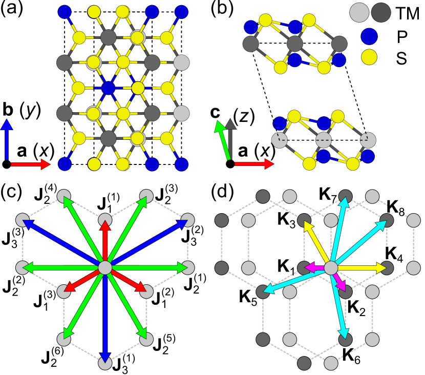
Figure 1: (a) Top view and (b) side view of the crystal structure of bulk TMPS₃’s. The global Cartesian axes (x, y and z) are defined such that the x and y directions coincide with the crystallographic direction a and b, respectively. (c) Intralayer and (d) interlayer exchange interactions considered.

The next is the single-ion anisotropy ($H_{\mathrm{SIA}}$):

$$H_{\mathrm{SIA}}=\sum_{i=1}^{N}{\mathbf{S}_{i}^{\mathsf{T}}\,\mathbf{D}\,\mathbf{S}_{i}},$$ (3)

where $\mathbf{D}$ is a symmetric matrix. In previous studies, a simpler version—diagonal $\mathbf{D}$ with $D_{xx}$ = $D_{yy}$ $\neq$ $D_{zz}$—has been used [16, 22].

In FePS₃, a coupling between orbital and spin polarizations ($LS$ coupling) leads to a strong magnetic anisotropy whose magnitude is about a few tens of meV [16], estimated from experimental results using crystal field theory. We therefore considered the following on-site contribution:

$$H_{LS}=\lambda{}\sum_{i=1}^{N}L_{iz}S_{iz},$$ (4)

where $\lambda$ represents the $LS$ coupling strength, and $L_{iz}$, which can be either $1$ or $-1$, is the magnetic quantum number for the orbital polarization of an Fe ion.

All the parameters of $H_{\text{exch}}^{\text{intra}}$, $H_{\text{exch}}^{\text{inter}}$, $H_{\text{SIA}}$, and $H_{LS}$ (eqs 1–4) were obtained based on DFT+$U$ calculations; see Supporting Information (SI) for calculation details of the anisotropic magnetic models.

Because the usual DFT(+$U$) methods cannot properly account for the dipolar coupling between local magnetic moments [23], we included the dipolar anisotropy ($H_{\rm dip}$) as the last constituent of our magnetic model:

$$H_{\mathrm{dip}}=\frac{1}{2}\sum_{i=1}^{N}\sum_{j=1,j\neq{}i}^{N}{}\left[\frac{\mathbf{m}_{i}\cdot\mathbf{m}_{j}}{r_{ij}^{3}}-\frac{3(\mathbf{m}_{i}\cdot\mathbf{r}_{ij})(\mathbf{m}_{j}\cdot\mathbf{r}_{ij})}{r_{ij}^{5}}\right],$$ (5)

where $\mathbf{m}_{i}$ and $\mathbf{m}_{j}$ are the local magnetic moments at the $i$-th and $j$-th sites, and $r_{ij}$ is the distance between $\mathbf{m}_{i}$ and $\mathbf{m}_{j}$; see SI for computational details of $H_{\mathrm{dip}}$.

Remarkably, the ground-state ordering patterns and the directions of spin moments of all three compounds obtained from our first-principles calculations (Figures 2a–c) agree perfectly with those obtained from neutron scattering experiments [24, 25, 26, 27].

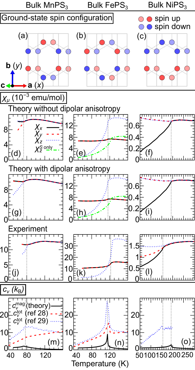
Figure 2: (a)–(c) The calculated ground-state spin-ordering pattern of bulk TMPS₃’s. (d)–(l) The magnetic susceptibility of bulk TMPS₃’s. The upper [(d)–(f)] and middle [(g)–(i)] panels show our calculation results, respectively, without and with considering the dipolar anisotropy. The lower [(j)–(l)] panels show the measured magnetic susceptibilities for bulk MnPS₃ and FePS₃ [16] and for bulk NiPS₃ [26]. In the case of FePS₃ [(e) and (h)], $\chi_{z}$ includes the effects of orbital polarizations (see also SI for computational details). (m)–(o) The calculated (magnetic) specific heat $c_{v}^{\mathrm{mag}}$ of bulk TMPS₃’s and the experimental data for the (total) specific heat $c_{v}^{\textrm{tot}}$ [28, 29]. The vertical dashed lines show the estimated critical temperatures.

Table 1 summarizes the contributions of $H_{\mathrm{exch}}^{\mathrm{intra}}$, $H_{\mathrm{exch}}^{\mathrm{inter}}$, $H_{\mathrm{SIA}}$, $H_{LS}$ and $H_{\mathrm{dip}}$ to the magnetic anisotropy of bulk TMPS₃. (i) In the case of MnPS₃, $H_{\mathrm{dip}}$ and $H_{\mathrm{SIA}}$ dominantly contribute to the magnetic anisotropy. These two contributions are of opposite (easy-axis and easy-plane, respectively) types and their sum results in a small easy-axis anisotropy (12.7 $\muup$eV) along $z$. Similar conclusions were drawn from previous experiments [30, 31]. (ii) In the case of FePS₃, $H_{LS}$ dominantly gives rise to a strong easy-axis anisotropy (20.6 meV) along $z$. The calculated $LS$ coupling strength $\lambda$ (10.2 meV) matches well with the $\lambda$ obtained from measured paramagnetic susceptibility (11.1–11.5 meV) [16]. (iii) In the case of NiPS₃, the contributions of $H_{\mathrm{SIA}}$, $H_{\mathrm{exch}}^{\mathrm{intra}}$ and $H_{\mathrm{dip}}$ are similar in magnitude. Their sum results in an easy-axis anisotropy (112.5 $\muup$eV) along $x$. While some studies claimed that NiPS₃ is best described by an XXZ model with easy-plane anisotropy [16, 7], our calculation results support the neutron scattering studies reporting an easy-axis anisotropy of a few hundred $\muup$eV [22] and the ordering direction of almost along $x$ [26].

	$\mathbf{n}$	$H_{LS}$	$H_{\rm SIA}$	$H_{\rm exch}^{\rm intra}$	$H_{\rm exch}^{\rm inter}$	$H_{\rm dip}$	$H_{\rm tot}$
MnPS3	$x$	0	$-$13.5	$-$1.4	0.1	18.6	3.8
	$y$	0	$-$14.3	$-$1.4	$-$0.1	17.6	1.6
	$z$	0.2	27.7	3.0	0.0	$-$36.2	$\mathbf{-5.3}$	(z)
FePS3	$x$	0	$-$10	404	15.6	$-$44.4	365
	$y$	0	$-$124	$-$120	$-$1.0	33.8	$-$211
	$z$	$-$20416	134	$-$284	$-$14.5	10.6	$\mathbf{-20567}$	(z)
NiPS3	$x$	0	$-$38.7	$-$21.1	$-$2.9	$-$11.9	$-\mathbf{74.6}$	(x)
	$y$	0	$-$21.0	45.7	$-$0.2	12.4	36.9
	$z$	$-$15	59.8	$-$24.6	3.2	0.6	39.0

Table 1: Magnetic anisotropy of bulk TMPS₃’s. The total energy ($H_{\text{tot}}$, the sum of eqs 1–5) per transition metal ion at a given ordering direction $\mathbf{n}$ ($x$, $y$ and $z$ in Figures 1a,b) is shown in units of $\muup$eV. The parenthesis in the last column shows the easy axis. The contributions of intralayer ($H_{\text{exch}}^{\text{intra}}$) and interlayer ($H_{\text{exch}}^{\text{inter}}$) exchange interactions, single-ion anisotropy ($H_{\text{SIA}}$), $LS$ coupling ($H_{LS}$), and dipolar anisotropy ($H_{\text{dip}}$) (eqs 1–5) are also shown.

Table 2 summarizes the isotropic intralayer exchange interaction $J_{n}^{(a)}(=1/3\,{\rm Tr}\,\mathbf{J}_{n}^{(a)}$) obtained from our calculations (here, the subscript $n$ in $J_{n}^{(a)}$ denotes the $n$-th nearest neighbor). For each $n$, there are two groups of $J_{n}^{(a)}$, e.g. $J_{1}^{(1)}$ and $J_{1}^{(2,3)}$, which are distinguished by the $C2/m$ symmetry of the crystal. These two groups should have different values for the isotropic exchange interactions in principle. However, since the distortion from a perfect honeycomb lattice is small, the difference between the two different values of $J_{n}^{(a)}$ turns out to be small for all $n$’s.

	$J_{1}^{(1)}$	$J_{1}^{(2,3)}$	$J_{2}^{(1,2)}$	$J_{2}^{(3\text{--}6)}$	$J_{3}^{(1)}$	$J_{3}^{(2,3)}$
MnPS3	1.06	1.18	0.07	0.07	0.72	0.69
FePS3	$-$1.36	$-$1.36	0.11	0.12	2.37	2.40
NiPS3	$-$5.21	$-$5.34	$-$0.23	$-$0.20	27.4	28.2

Table 2: Isotropic intralayer exchange interaction $J_{n}^{(a)}=1/3\,\mathrm{Tr}\,\mathbf{J}_{n}^{(a)}$ in units of meV (see Figure 1c also).

In the case of MnPS₃ and FePS₃, the calculated $J_{n}^{(a)}$’s are in good agreement with neutron scattering experiments [22]. In the case of NiPS₃, $J_{3}^{(1\text{--}3)}$ obtained from our calculations are larger than the value fitted with a model to experimental results, $J_{3}$ = 13.8 meV [22]. (Here, we doubled this value in order to compensate the difference in the definition of $J_{3}$ in ref 22 and in this study.) A rough estimate of the spin-wave gap in NiPS₃ is $\sim$ $2S\sqrt{3\Delta J_{3}}$ [22], where $\Delta$ is the single parameter that represents the total magnetic anisotropy energy per transition metal ion. Putting $J_{3}$ = 28 meV (Table 2), and $\Delta$ = 0.11 meV (the magnitude of the easy-axis anisotropy in NiPS₃, see Table 1) into the expression for the spin-wave gap yields 6.1 meV, which is very close to the measured spin-wave gap (7 meV) [22]. $J_{3}$ used in the experimental study is an intermediate parameter, which is indirectly estimated by a fitting procedure. On the other hand, the spin-wave gap is a directly measured quantity from neutron scattering spectra, and our calculations explain this measured gap quite well.

The classical Monte Carlo method, describing the magnetic ordering of ferromagnetic 2D materials well [32, 33], was employed in our study on the temperature and thickness dependence of the thermodynamic quantities of TMPS₃’s; see SI for discussions on the validity of using the classical Monte Carlo simulation. Figures 2d–l show the magnetic susceptibility of bulk TMPS₃’s. The calculated $T_{\text{N}}$’s of MnPS₃ and FePS₃ are 72 K and 116 K, respectively, in good agreement with experiments (80 K and 120 K, respectively) [21, 16]. In the case of MnPS₃ (Figure 2g), not only the $T_{\text{N}}$ but also the anisotropy of the magnetic susceptibility (the differences between $\chi_{x}$, $\chi_{y}$ and $\chi_{z}$) agrees with the experimental data (Figure 2j). As can be seen in Figures 2d and g, $H_{\text{dip}}$ plays a crucial role in reproducing the anisotropy of the magnetic susceptibility below $T_{\text{N}}$. Quite remarkably, in the case of FePS₃ (Figure 2h), the calculated magnetic susceptibilities reproduce the significant difference between $\chi_{z}$ and $\chi_{x,y}$ over all temperatures, in agreement with the experiment (Figure 2k). Here, we emphasize the importance of including the orbital degrees of freedom ($L_{iz}$ in eq 4) in calculating the magnetic susceptibility: the significant enhancement of $\chi_{z}$ shown in Figures 2e and h (see also SI for how the orbital contribution was considered in our Monte Carlo simulations).

In the case of NiPS₃ (Figure 2i), although the calculated $T_{\text{N}}$ (193 K) is 38 K higher than the experimental value (155 K) [16, 26], it is in much better agreement with experiments than previous theoretical estimations (353 K and 560 K from refs 22 and 34, respectively). More importantly, our calculations reproduce several key features observed in experiments: (i) the susceptibility is very isotropic ($\chi_{x}=\chi_{y}=\chi_{z}$) if $T>T_{\text{N}}$, (ii) there is a broad peak far above $T_{\text{N}}$ at $T\sim$250 K, and (iii) $\chi_{x}$ is the smallest if $T<T_{\text{N}}$, indicating that the antiferromagnetic order is almost along $x$ [26, 22].

Figures 2m–o show the magnetic specific heat ($c_{v}^{\mathrm{mag}}$) of bulk TMPS₃. The peak in the $c_{v}^{\text{mag}}$ of FePS₃ is much sharper than those in the other cases, in good agreement with experiments [28, 29], which is easily understood in that the magnetic anisotropy of FePS₃ is orders of magnitude larger than that of the other TMPS₃’s (Table 1). We note that the measured total specific heat ($c_{v}^{\mathrm{tot}}$) for bulk TMPS₃ shown in Figures 2m–o includes the contributions arising from phonons and other possible noises and that the discrepancies between the different experimental results call for further experimental studies guided by our paper.

Now we discuss how the $T_{\text{N}}$ and magnetic susceptibility change with the number of layers in few-layer FePS₃ and NiPS₃. In Figure 3, we first notice that the magnetic phase transition exists in the monolayer (1L) limit. The thickness dependence of the $T_{\text{N}}$ significantly varies with the transition metal element. In the case of FePS₃, the $T_{\text{N}}$ is (almost) independent of the number of layers, also in good agreement with experiments [6]. The interlayer exchange interactions in FePS₃ (see SI Table S1) are orders of magnitude smaller than the intralayer ones (Table 2) and the $LS$ coupling (see Table 1); this explains why the $T_{\text{N}}$ hardly changes with the thickness.

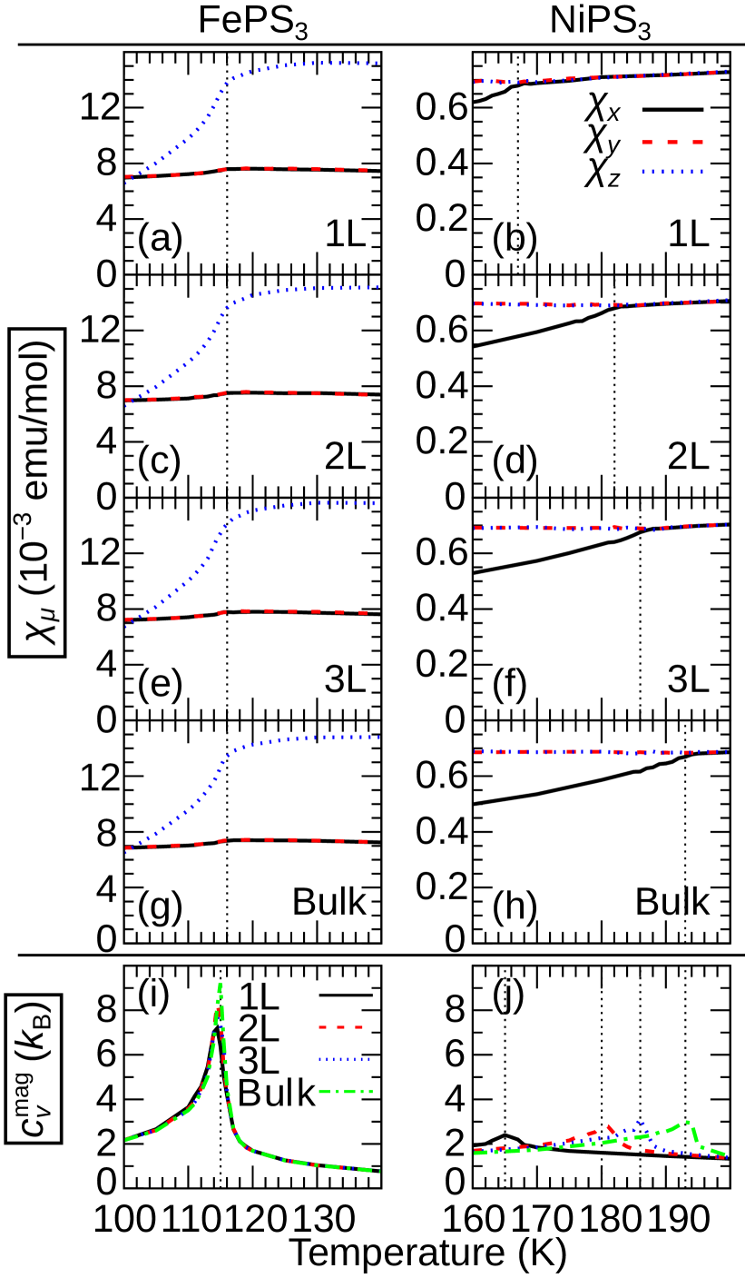
Figure 3: (a)–(h) The magnetic susceptibility of bulk and few-layer TMPS₃’s. (i)–(j) The specific heat arising from magnetic moments $c_{v}^{\mathrm{mag}}$ of bulk and few-layer TMPS₃’s. The vertical dashed lines show the estimated Néel temperatures.

By contrast, $T_{\text{N}}^{\mathrm{bulk}}-T_{\text{N}}^{\mathrm{1L}}$ of NiPS₃ (28 K) is much larger than that of FePS₃ (0 K); this is easily explained by the unusually large interlayer exchange interactions of NiPS₃, especially the second-nearest-neighbor ones ($K_{3,4}$ =$1/3\,\mathrm{Tr}\,\mathbf{K}_{3,4}$ $\sim$ 1.64 meV, see SI Table S1), which are as large as 30 % of the nearest-neighbor intralayer exchange interactions ($J_{1}^{(1\text{--}3)}$ $\sim$ $-$5.3 meV, see Table 2).

Notably, we predict a finite (and also considerably large) $T_{\mathrm{N}}$ for monolayer NiPS₃ (Figures 3b and j), which indicates that the magnetic order persists in the genuine 2D limit of NiPS₃. On the other hand, a recent Raman study drew exactly the opposite conclusion that the magnetic order is absent in monolayer NiPS₃ (but is present in bilayer or thicker samples) [7], which was largely based on their observation that the frequencies of certain Raman peaks (denoted as P₂ in ref 7, the $E_{g}$ modes at $\sim$180 cm^-1) did not budge with decreasing the temperature (far below the bulk $T_{\mathrm{N}}$) in monolayer samples while noticeably shifted in thicker samples.

At the same time, ref 7 also reported the emergence of a strong two-magnon continuum in the Raman spectrum of monolayer NiPS₃, which is a clear evidence of magnetic ordering, at similar temperatures as in thicker samples. Thus, the two seemingly contradictory experimental results have remained a puzzle so far.

Remarkably, we found that such a complete absence of the frequency shifts of P₂ peaks in the Raman spectrum of magnetically-ordered monolayer NiPS₃ can be fully understood if the effects of the three-fold-degenerate ground-state manifold of monolayer NiPS₃, as in other honeycomb-lattice compounds [35], is considered. Our resolution of this important puzzle, together with the results of our calculations, fully explains the seemingly contradictory experimental results in ref 7 but, at the same time, disproves the conclusion therein.

In the previous Raman study [7], a pair of degenerate Raman peaks (labeled as P₂ in ref 7), one of which was only visible in the parallel-polarization setup [$-z(xx)z$] and the other only in the cross-polarization setup [$-z(xy)z$], was considered an order parameter of bulk NiPS₃ because a frequency difference between the two Raman peaks (denoted as $\Delta$P₂ from now on) started to develop just below $T_{\mathrm{N}}$ and increased further as the temperature decreased while $\Delta$P₂ was negligible above $T_{\mathrm{N}}$. The same phenomenon was observed from the bulk down to the bilayer. In monolayers on the other hand, $\Delta$P₂ remained zero at all temperatures. The result was then interpreted that the magnetic order is absent only in monolayer NiPS₃.

However, we realized that $\Delta$P₂ cannot be measured from Raman experiments with the two (parallel- and cross-) polarization setups even if the magnetic order persists in monolayer NiPS₃. A monolayer NiPS₃ has a three-fold rotation symmetry (the $D_{3d}$ point group) due to the lack of monoclinic stacking; consequently, its zigzag antiferromagnetic ground states are triply degenerated (imagine three different zigzag directions that can fit in a honeycomb lattice). An important note here is that all three degenerate states appear in a sample as magnetic domains with three different optical responses (this phenomenon is common in compounds with three-fold ground states interconnected by three-fold rotations [35]). The Raman responses of such domains should be averaged when we discuss the polarization-setup dependence of Raman peaks in monolayer NiPS₃.

The two P₂ peaks are assigned to the $E_{g}$ phonon mode in the $D_{3d}$ point group and their Raman tensors, which we will denote as $E_{g}^{(1)}$ and $E_{g}^{(2)}$, are respectively given by

$$\begin{pmatrix}c&0&0\\ 0&-c&d\\ 0&d&0\end{pmatrix}\,\mathrm{and}\,\begin{pmatrix}0&-c&-d\\ -c&0&0\\ -d&0&0\end{pmatrix},$$ (6)

where $c$ and $d$ are real numbers. The Raman intensities in the parallel- and cross-polarization setups are proportional to the squares of the $xx$ and $xy$ components of the Raman tensors, respectively. The $E_{g}^{(1)}$ mode is therefore visible only in the parallel-polarization setup while the $E_{g}^{(2)}$ mode only in the cross-polarization setup. If magnetic ordering happens, a frequency difference between the two modes develops. Since the Raman peaks can be selectively captured (by adjusting the polarizations of incoming and outgoing lights), $\Delta$P₂ can be measured accurately no matter how broad each of the two P₂ peaks is (see Figure 4a).

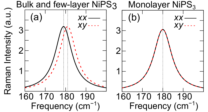
Figure 4: Simulated Raman spectra of NiPS₃ near the P₂ peaks for (a) few-layer and bulk NiPS₃ (the $C_{2h}$ point group) and (b) monolayer NiPS₃ (the $D_{3d}$ point group). It was assumed that the two peaks comprising P₂ are given by Lorentzians with the same height and width and their centers are separated by 2 cm^-1. The half-width at half-maximum is 5 cm^-1. These parameters were chosen to mimic the experimental results [7]. In the legends, $xx$ and $xy$ represent the parallel- and cross-polarization setups, respectively.

Note, however, that those Raman tensors are for one of the three zigzag orientations where the same-spin zigzag chains are aligned along the $x$ direction. The Raman tensors for the other zigzag orientations can be obtained by applying 120^∘ and 240^∘ rotations with respect to $z$ to the above expressions. In the case of the $E_{g}^{(1)}$ mode, the Raman tensors for all the different orientations are written as

$$\begin{pmatrix}c&0&0\\ 0&-c&d\\ 0&d&0\end{pmatrix}\,,\,\begin{pmatrix}-\frac{c}{2}&-\frac{\sqrt{3}c}{2}&-\frac{\sqrt{3}d}{2}\\ -\frac{\sqrt{3}c}{2}&\frac{c}{2}&-\frac{d}{2}\\ -\frac{\sqrt{3}d}{2}&-\frac{d}{2}&0\end{pmatrix}\,,\mathrm{and}\,\begin{pmatrix}-\frac{c}{2}&\frac{\sqrt{3}c}{2}&\frac{\sqrt{3}d}{2}\\ \frac{\sqrt{3}c}{2}&\frac{c}{2}&-\frac{d}{2}\\ \frac{\sqrt{3}d}{2}&-\frac{d}{2}&0\end{pmatrix}.$$ (7)

Similarly, the three $E_{g}^{(2)}$ Raman tensors for the three different zigzag orientations read

$$\begin{pmatrix}0&-c&-d\\ -c&0&0\\ -d&0&0\end{pmatrix}\,,\,\begin{pmatrix}\frac{\sqrt{3}c}{2}&\frac{c}{2}&\frac{d}{2}\\ \frac{c}{2}&-\frac{\sqrt{3}c}{2}&\frac{\sqrt{3}d}{2}\\ \frac{d}{2}&\frac{\sqrt{3}d}{2}&0\end{pmatrix}\,,\mathrm{and}\,\begin{pmatrix}-\frac{\sqrt{3}c}{2}&\frac{c}{2}&\frac{d}{2}\\ \frac{c}{2}&\frac{\sqrt{3}c}{2}&-\frac{\sqrt{3}d}{2}\\ \frac{d}{2}&-\frac{\sqrt{3}d}{2}&0\end{pmatrix}.$$ (8)

Element-wise square-averaging of the Raman tensors over the three zigzag orientations now yields the following intensity matrices

$$\begin{pmatrix}\frac{c^{2}}{2}&\frac{c^{2}}{2}&\frac{d^{2}}{2}\\ \frac{c^{2}}{2}&\frac{c^{2}}{2}&\frac{d^{2}}{2}\\ \frac{d^{2}}{2}&\frac{d^{2}}{2}&0\end{pmatrix}\,\mathrm{and}\,\begin{pmatrix}\frac{c^{2}}{2}&\frac{c^{2}}{2}&\frac{d^{2}}{2}\\ \frac{c^{2}}{2}&\frac{c^{2}}{2}&\frac{d^{2}}{2}\\ \frac{d^{2}}{2}&\frac{d^{2}}{2}&0\end{pmatrix},$$ (9)

respectively, for $E_{g}^{(1)}$ and $E_{g}^{(2)}$. Here, the $xx$ ($xy$) components of these two matrices give the domain-averaged Raman intensities for $E_{g}^{(1)}$ and $E_{g}^{(2)}$, respectively, in the parallel (cross) polarization setup. Remarkably, (i) these two matrices are exactly the same and (ii) their $xx$ and $xy$ components are also the same. An important point here is that there is certainly no polarization selection rule for the $E_{g}^{(1)}$ and $E_{g}^{(2)}$ modes if the averaging effects of the magnetic domains are taken into account: the two peaks comprising the P₂ peak are to be observed with equal intensities regardless of whether the parallel- or cross-polarization setup is used.

Such a disappearance of the polarization-setup dependence has a huge impact on detecting $\Delta$P₂ in practice; the impact is much more dramatic when the broadness of the two peaks comprising the P₂ peak is similar to or even larger than their frequency difference ($\Delta$P₂). If that condition is met, the two peaks appear to be just one peak. Unfortunately, the splitting in the peaks $\Delta$P₂ measured in ref 7 were at most $\sim$2 cm^-1 (in few-layer and bulk NiPS₃), and the half-width at half-maximum of the P₂ peaks in monolayer NiPS₃ were at least 5 cm^-1. Given that condition, $\Delta$P₂ cannot be measured because of the large overlap between the peaks as shown in Figure 4b.

In summary, our anisotropic magnetic model with an unprecedentedly large number of parameters determined from extensive first-principles calculations and classical Monte Carlo simulations with special handling of the orbital polarization effects explained the magnetic structure, critical temperature, susceptibility, and specific heat of bulk and few-layer TMPS₃’s reported from experiments. Moreover, we have shown that the criterion used to judge magnetic ordering in the recent Raman study of NiPS₃ [7] is invalid in the case of monolayer samples and that magnetic ordering in NiPS₃ persists down to the monolayer limit. Recently, direct measurements of the magnetic susceptibility of 2D materials were carried out [36]. Thus, our predictions on the thickness dependence of the thermodynamic quantities of few-layer TMPS₃’s can be verified immediately, which will allow a deeper understanding of magnetic ordering in atomically-thin 2D materials, a fundamental issue of the Mermin-Wagner theorem [13].

Appendix A Calculation details: anisotropic magnetic model from constrained DFT+$U$ calculations

A.1 Anisotropic magnetic model

In this section, we describe how the anisotropic magnetic model $H_{\rm tot}$, which is given by

$$H_{\rm tot} =\frac{1}{2}\sum_{i=1}^{N}\sum_{n=1}^{3}\sum_{a=1}^{M_{n}}{\mathbf{S}_{i}^{\mathsf{T}}\,\mathbf{J}_{n}^{(a)}\,\mathbf{S}_{j(i,\mathbf{J}_{n}^{(a)})}}+\frac{1}{2}\sum_{i=1}^{N}\sum_{n=1}^{8}{\mathbf{S}_{i}^{\mathsf{T}}\,\mathbf{K}_{n}\,\mathbf{S}_{j(i,\mathbf{K}_{n})}}$$

$$+\sum_{i=1}^{N}{\mathbf{S}_{i}^{\mathsf{T}}\,\mathbf{D}\,\mathbf{S}_{i}}+\sum_{i=1}^{N}\lambda L_{iz}S_{iz}+H_{\rm dip}\,,$$ (A10)

was determined from first-principles calculations. The $C2/m$ symmetry of the crystal structure of TMPS₃ was considered to restrict matrices $\mathbf{J}_{n}^{(a)}$, $\mathbf{K}_{n}$, and $\mathbf{D}$: (i) $\mathbf{J}_{1}^{(1)}$, $\mathbf{J}_{2}^{(1,2)}$, $\mathbf{J}_{3}^{(1)}$, $\mathbf{K}_{1}$, $\mathbf{K}_{4}$, and $\mathbf{D}$ are of the form

$$\begin{pmatrix}a&0&d\\ 0&b&0\\ d&0&c\end{pmatrix}\,,$$ (A11)

and (ii) the other matrices in eq A10 are of the form

$$\begin{pmatrix}a&e&d\\ e&b&f\\ d&f&c\end{pmatrix}\,,$$ (A12)

where $a$, $b$, $c$, $\cdots$, and $f$ are real numbers.

A.2 Total energy mapping analysis

To obtain the parameters in eq A10, we first calculated the total energies of bilayer TMPS₃’s with different magnetic patterns and different collinear directions. Figure S1 shows the collinear magnetic ordering patterns for which DFT+$U$ total energies were calculated. We mention that the lowest-energy configurations obtained from our first-principles calculations coincide with the ordering patterns for all three bulk TMPS₃ compounds reported from neutron scattering experiments: the patterns of Figures S1c, g, and f for MnPS₃ [24], FePS₃ [24, 25], and NiPS₃ [26], respectively. For each ordering pattern in Figure S1, six different collinear directions were chosen, which means in total 132 total energy calculations were carried out for each TMPS₃. With the $C2/m$ symmetry fully considered, the total energies are then used to obtain 73 free parameters for each TMPS₃ using the least square method. We note that for some of 22 ordering patterns depicted in Figure S1 the total energy was not employed as itself in the fitting procedure: For the ordering patterns in Figures S1e, j, and o, the difference between the total energies of the two ordering patterns was used; For the ordering patterns in Figure S1p, a specific combination of pluses and minuses of the total energies of the four ordering patterns was used as this particular choice gives the difference between $\mathbf{J}_{3}^{(1)}$ and $\mathbf{J}_{3}^{(2,3)}$. The spin directions of the transition metal ions were constrained to be along the collinear directions during the total energy calculations. In the case of MnPS₃ and NiPS₃, the collinear direction $\mathbf{n}$ was chosen to be [1, 0, 0]^T, [0, 1, 0]^T, [0, 0, 1]^T, [$\mathrm{sin}\,\theta$, 0, $\mathrm{cos}\,\theta$]^T, [0, $\mathrm{sin}\,\theta$, $\mathrm{cos}\,\theta$]^T, and [$\mathrm{cos}\,\phi$, $\mathrm{sin}\,\phi$, 0]^T (in Cartesian coordinates), where $\theta=30^{\circ}$ and $\phi=30^{\circ}$. In the case of FePS₃, a different choice for $\mathbf{n}$ was made to more accurately capture the magnetic anisotropy that strongly favors the $z$ direction: $\mathbf{n}$ = [$\mathrm{sin}\,\theta_{1}$, 0, $\mathrm{cos}\,\theta_{1}$]^T, [0, $\mathrm{sin}\,\theta_{1}$, $\mathrm{cos}\,\theta_{1}$]^T, [0, 0, 1]^T, [$\mathrm{sin}\,\theta_{2}$, 0, $\mathrm{cos}\,\theta_{2}$]^T, [0, $\mathrm{sin}\,\theta_{2}$, $\mathrm{cos}\,\theta_{2}$]^T, and [$\mathrm{sin}\,\theta_{2}\,\mathrm{cos}\,\phi$, $\mathrm{sin}\,\theta_{2}\,\mathrm{sin}\,\phi$, $\mathrm{cos}\,\theta_{2}$]^T, where $\theta_{1}=30^{\circ}$, $\theta_{2}=60^{\circ}$, and $\phi=30^{\circ}$.

A.3 Constrained DFT+$U$ calculations

We carried out DFT+$U$ calculations using our custom version of Quantum ESPRESSO suite [37], in which we implemented a scheme that constrains the spin directions as proposed in ref 38 with our adaptations for the DFT+$U$ method. In our implementation, the local magnetic moment at the $i$-th magnetic atom $\mathbf{m}_{i}$ was chosen to be

$$\mathbf{m}_{i}=\sum_{s_{1}s_{2}}\sum_{m}\sum_{n\mathbf{k}}\left<\psi_{n\mathbf{k}}^{s_{1}}\big{|}\phi_{im}\right>{\bm{\sigma}}_{s_{1}s_{2}}\left<\phi_{im}\big{|}\psi_{n\mathbf{k}}^{s_{2}}\right>,$$ (A13)

where $s_{1}$ and $s_{2}$ are the spinor indices, $\left|\psi_{n\mathbf{k}}^{s}\right>$ is the spin $s$ component of the Kohn-Sham spinor wavefunction with the band index $n$ and momentum $\mathbf{k}$, $\left|\phi_{im}\right>$ is the $3d$ atomic orbital of the $i$-th magnetic atom with the orbital magnetic quantum number $m$, and ${\bm{\sigma}}_{s_{1}s_{2}}$ is the $(s_{1},s_{2})$ component of the Pauli matrices ${\bm{\sigma}}=(\sigma^{x},\sigma^{y},\sigma^{z})$. Then the spin direction of the magnetic atom is constrained along a predefined direction $\mathbf{e}_{i}$ by minimizing the DFT total energy plus the penalty energy given as [38]

$$E_{p}=\sum_{i}\lambda_{i}\left(\left|\mathbf{m}_{i}\right|-\mathbf{e}_{i}\cdot\mathbf{m}_{i}\right),$$ (A14)

where $\lambda_{i}$ determines how close the constrained spin direction of $\mathbf{m}_{i}$ will be to $\mathbf{e}_{i}$. In our calculations $\lambda_{i}$ was typically set to 1 Ry, which yielded well-converged local magnetic moments, $\mathbf{m}_{i}$’s, close to their target directions, $\mathbf{e}_{i}$’s.

A.4 Further computational details

The exchange-correlation functional within the local density approximation (LDA) parametrized by Perdew and Zunger [39] was used to calculate the exchange-correlation energy. We employed a rotationally invariant LDA+$U$ method suggested by Liechtenstein et al . [40]. The effective Coulomb interaction $U$ was set to 6.5 eV and 4 eV for NiPS₃ and the other TMPS₃’s, respectively. In determining the $U$ values, we first tested several different $U$ values in the range 3–7 eV and chose the values that provide reasonable estimates for the $T_{\mathrm{N}}$ of the bulk TMPS₃ compounds. We then carried out linear response calculations with the hp.x program [41] in the Quantum ESPRESSO suite to see whether those empirical $U$ values could be supported by the well-established framework for computing $U$ values from first principles. Our linear response calculations yielded 2.9 eV, 3.9 eV, and 6.6 eV for the transition metal elements in MnPS₃, FePS₃, and NiPS₃, respectively, which are in good agreement with our empirically chosen $U$ values. In general, $U$ tends to increase across the row in the periodic table (from left to right) as the 3$d$ electrons get more localized [42]. In terms of $U$, therefore, CoPS₃ ($Z$=27 for Co) is expected to be somewhere between FePS₃ ($Z$=26 for Fe) and NiPS₃ ($Z$=28 for Ni); that would explain the gap between the $U$ of FePS₃ and that of NiPS₃.

Optimized, norm-conserving pseudopotentials [43, 44] that include the relativistic effects were used to simulate the interactions between the nuclei and electrons. The kinetic energy cutoff of the plane-wave basis was set to 80 Ry.

The atomic coordinates of a bilayer TMPS₃ were adopted from the atomic coordinates of the bulk structure reported from an experimental study [45]. Because of the over-binding behavior of the LDA, we did not carry out further structural relaxations. This over-binding behavior of the LDA has always been a notorious problem because a physical property of a material is often sensitive to its geometry. And when the LDA fails to provide a reasonable result for the structure, as it really does in the case of TMPS₃ as well as in the cases of many other materials, there is no way but to resort to the experimental structure since a structural relaxation with the LDA plus a van der Waals correction is not a viable option since all the available van der Waals correction methods are designed to work with the GGA. (In Section A.5 of this Supporting Information, we show why we chose to use the LDA and not the GGA.) Fortunately, keeping the experimental structure is known to give good results for the magnetic properties [46, 47, 48, 49, 50, 51], which are the main focus of our study, and we therefore used the experimental structure. To avoid spurious interactions between periodic images, a vacuum layer with 18 Å thickness was placed between the adjacent periodic images.

We calculated the total energy for a supercell (Figure S1) having $N_{1}\times N_{2}\times 1$ unit cells of nonmagnetic TMPS₃ (Figure S2), where ($N_{1}$, $N_{2}$) is (1, 1), (2, 1), (1, 2), (4, 1), and (1, 4). To keep the $k$-point density in the reciprocal space for the calculations involving supercells of different size the same, we used an $8/N_{1}\times 8/N_{2}\times 1$ Monkhorst-Pack grid [52] in the case of the $N_{1}\times N_{2}\times 1$-supercell calculations.

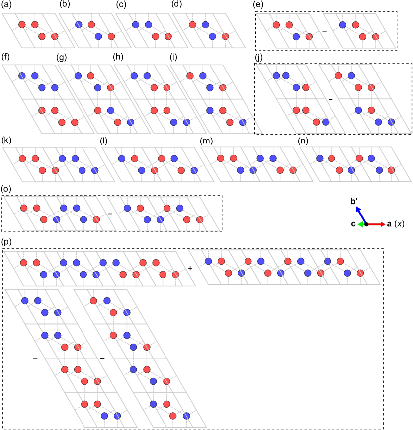
Figure S1: Top view of the collinear magnetic patterns of bilayer TMPS₃ used to calculate the parameters of the anisotropic magnetic model (eq A10). The red and blue disks represent the spin-up and spin-down transition metal ions, respectively, with respect to the collinear direction.

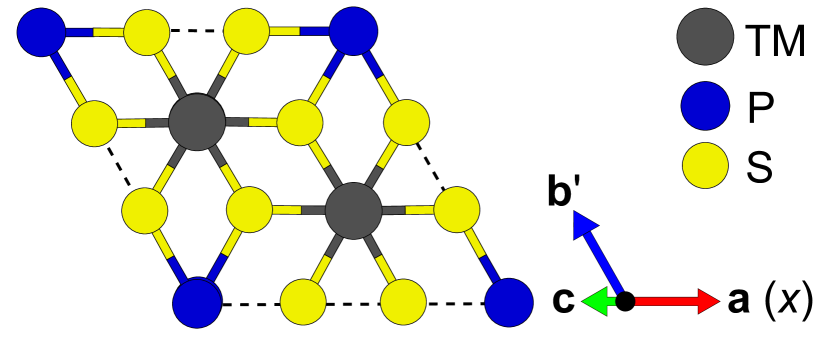
Figure S2: Top view of the primitive unit cell of nonmagnetic TMPS₃.

A.5 Note on exchange-correlation functional with non-collinear magnetism

In this work, we did not use the generalized gradient approximation (GGA) because the GGA with noncollinear magnetism (GGA+NCM) causes severe numerical instabilities (note that we need NCM thanks to spin-orbit coupling); with the GGA+NCM, we were not able to reach the level of accuracy needed to resolve the magnetic anisotropy energy, which could be as small as a few tens of $\muup$eV per transition metal atom. The GGA+NCM, of which a widely adopted formulation was proposed in ref 53, has “both formal and numerical problems” [54]. The computational issue most likely emerges from small regions in space where spin density is close to zero. Here, if the local spin polarization changes slowly in space passing through zero, its direction is reverted. This reversal in the direction of the local spin polarization is not a big deal in reality because the magnitude of the local spin polarization is zero. One remarkable peculiarity of the GGA+NCM is that even if the spin density changes smoothly over such regions, the GGA+NCM functional recognizes it as a kink, the gradient of which is singular, thus causing severe numerical instabilities.

We examined how this serious issue had been dealt with in some public software packages. Surprisingly, currently there is no systematic solution for these instabilities based on justifiable theory but only ad hoc methods have been made without sound theoretical justification. In the case of the Elk code [55], for example, the kinks were smoothed out by preventing the magnitude of magnetization density from being smaller than a threshold. We would have applied this prescription to our code if it had been possible to keep this threshold sufficiently small while attaining a reasonable degree of convergence. We found, however, that the threshold had to be fairly large for convergence, so that it would affect the small magnetic anisotropies that we wanted to determine as accurately as possible. In the case of VASP [56], this inherent instability of GGA+NCM can be dealt with by using its own variation (whose formal and conceptual validity is not discussed) different from the original formulation of ref 53. In passing we note that Quantum ESPRESSO did not make such ad hoc, unjustifiable compromises and hence it transparently shows the serious instability problem inherent in the GGA+NCM.

In fact, the numerical instability of the GGA+NCM is deeply related with its formal problem, as the scheme completely ignores the contribution to the exchange-correlation energy due to the gradient of magnetization density perpendicular to the local magnetization direction, while the exact exchange-correlation energy is certainly affected by that contribution [57]. There have been a few papers addressing this issue and proposing different formulations of the GGA+NCM [54, 58], but none of them really complied with the conditions that should be satisfied by the exact exchange-correlation energy; by the way, one of them has been retracted [59]. In contrast, the LDA is free from such issues. Therefore, we decided to use the LDA instead of the GGA to meet our strict criterion for convergence and to avoid the risk of being affected by those inherent problems of the GGA+NCM scheme.

Appendix B Calculation details: dipolar anisotropy

The contribution of the magnetic dipole-dipole interactions between localized magnetic moments to our magnetic model is given by the usual expression:

$$H_{\rm dip}=\frac{1}{2}\sum_{i=1}^{N}\sum_{j=1,j\neq{}i}^{N}\left[\frac{\mathbf{m}_{i}\cdot\mathbf{m}_{j}}{r_{ij}^{3}}-\frac{3(\mathbf{m}_{i}\cdot\mathbf{r}_{ij})(\mathbf{m}_{j}\cdot\mathbf{r}_{ij})}{r_{ij}^{5}}\right].$$ (B15)

The paramagnetic susceptibilities of MnPS₃ and NiPS₃ are well described by the spin-only magnetic moments of $S=2.5$ and $S=1$, respectively [16]. This indicates that $\mathbf{m}_{i}$ for MnPS₃ and NiPS₃ is given by $2\mu_{\rm B}\mathbf{S}_{i}$, where $\mu_{\rm B}$ is the Bohr magneton. In the case of FePS₃ ($S=2$), on the other hand, $\mathbf{m}_{i}$ is also contributed by the orbital polarizations. The $z$ component of $\mathbf{m}_{i}$ is now given by $m_{iz}=\mu_{\rm B}(2S_{iz}+L_{iz})$, while the $x$ and $y$ components have no orbital contributions and are given by $m_{ix}=2\mu_{\rm B}S_{ix}$ and $m_{iy}=2\mu_{\rm B}S_{iy}$, respectively. Because $H_{\rm dip}$ is negligibly small compared to the magnetic anisotropy arising from $LS$ coupling and a nonzero $L_{iz}$ ($=\pm 1$) affects only a fraction ($\sim$25%) of $m_{iz}$, whether the orbital contributions (the terms that include $L_{iz}$) of $H_{\rm dip}$ are exactly treated or not is of no importance at all in discussing the magnetic ordering of FePS₃. In our calculations, $H_{\rm dip}$ for FePS₃ was evaluated with $\mathbf{m}_{i}=2\mu_{\rm B}\mathbf{S}_{i}$ so that the spin-only part of $H_{\rm dip}$ was taken into account, but this term can also be dropped in investigating the magnetic ordering in FePS₃ (see the negligible difference between Figures 2e and h of the main manuscript).

Here, we further look into the effects of the dipolar anisotropy on the magnetic anisotropy of TMPS₃ by calculating $H_{\rm dip}$ for the ground-state magnetic configurations of bulk TMPS₃ (the configurations shown in Figures S1c, g, and f for MnPS₃, FePS₃, and NiPS₃, or, equivalently, in Figures 2a–c in the main manuscript, respectively) and examining the differences between the values of $H_{\rm dip}$ evaluated with imposing different collinear spin directions ($x$, $y$, and $z$) for $\mathbf{m}_{i}$’s. We circumvented the issue of dealing with summing over infinitely many pairs of the magnetic sites ($i$ and $j$ in eq B15) by neglecting the terms of which the distance between the spins $r_{ij}$ is longer than a certain cutoff $r_{\rm cut}$. The convergence of the dipolar anisotropy with respect to the cutoff distance was tested for several values of $r_{\rm cut}$ ranging from 5 Å to 50 Å.

As Figure S3 shows, the choice of $r_{\rm cut}$ = 9 Å yields reasonably converged results for the dipolar anisotropy of TMPS₃ (see the vertical dotted lines). In the case of MnPS₃ (Figure S3a), $H_{\rm dip}$ favors an easy-axis anisotropy along $z$. In the case of FePS₃ and NiPS₃ (Figures S3b and c), it gives rise to easy-axis anisotropies along the $x$ direction. The magnitude of the dipolar anisotropy is about a few tens of $\muup$eV, ranging between 10 $\muup$eV and 80 $\muup$eV, per transition metal ion.

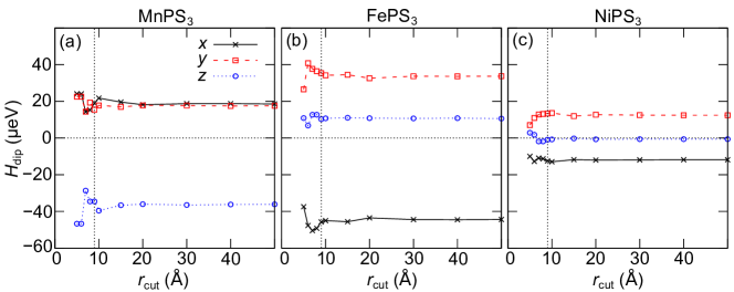
Figure S3: Convergence of the dipolar anisotropy, $H_{\rm dip}$ (eq B15) per transition metal ion, with respect to the cutoff distance $r_{\rm cut}$. The vertical dotted lines are placed at $r_{\rm cut}$ = 9 Å.

Appendix C Effects of LS coupling on the magnetic anisotropy energy and some related numerical issues

C.1 Effects of LS coupling in FePS₃

Given that $LS$ coupling dominantly contributes to the magnetic anisotropy of FePS₃, its (effective) functional form with respect to the orbital and spin polarizations can be assessed by looking at how the orbital polarization of an Fe ion and the total energy of the system change with the direction of the spin polarization. Here, we present a simple analysis based on our DFT+$U$ calculations using fully-relativistic pseudopotentials that can justify the specific form of the $LS$ coupling term, $\sum_{i=1}^{N}\lambda L_{iz}S_{iz}$, used in our magnetic model (eq A10).

We calculated the total energy of bilayer FePS₃ and the orbital polarization of an Fe ion within the system for ferromagnetic configurations (Figure S1a) of various collinear spin directions. The choice of using the ferromagnetic ordering is just for convenience, because then all the transition metal ions have the same orbital and spin polarizations ($L_{z}=L_{iz}$ and $S_{z}=S_{iz}$ for all $i$). We have checked that the results are essentially the same if we use the ground state magnetic configuration (Figure S1g).

Figure S4a shows the orbital polarization of an Fe ion as a function of the direction of its spin polarization. The $z$ component of the orbital polarization is unquenched and is almost constant ($L_{z}\sim 1$) as the spin rotates fully (by 360^∘ in the $yz$ plane as depicted) while the other components remain relatively small. Figure S4b displays the effect of this unquenched $L_{z}$ on the magnetic anisotropy. It shows the total energy of the magnetic configurations with $L_{z}\approx 1$ and $L_{z}\approx-1$. At $\theta$ = 90^∘, where the spin lies in the $xy$ plane, there is a cusp in the lowest-energy curve (the dash-dotted blue curve in Figure S4b), which is a direct consequence of the two-fold degeneracy arising from the orbital degrees of freedom ($L_{z}$ being either 1 or $-$1). This $\left|\cos\theta\right|$ dependence on the collinear spin direction is differentiated from the usual $\cos^{2}\theta$ dependence of the contributions arising from the other terms in eq A10. A similar analysis was done for the ground-state magnetic configuration (Figure S1h or, equivalently, Figure 2b in the main manuscript) and the same $\left|\cos\theta\right|$ dependence was obtained.

We note that a delicate handling of the initial occupation matrix was required especially when we tried to calculate the total energy for the magnetic configurations whose local spins were aligned with the hard axes, the $x$ and $y$ directions. And this numerical issue is closely related to the two-fold degeneracy shown at $\theta$ = 90^∘ and 270^∘ in Figure S4b. We had to initialize the occupation matrix with complex numbers so that the initial occupation matrix had unquenched orbital angular momentum (e.g. $L_{z}$ = $\pm 1$), and only through that way the correct, orbital-polarized ground states were obtained. Since filling the initial occupation matrix with complex numbers is not the common practice for LDA+$U$ calculations, it is likely that even experts in first-principles calculations might have missed this delicate total energy minimum.

C.2 Failure of magnetic force theorem

The influence of orbital degrees of freedom is not restricted to the sensitiveness to the initial condition on the occupation matrix. What is more important is that it excludes the use of the magnetic force theorem (MFT) [60] from consideration. Since knowing how the MFT is working is important to understand why it should not be used in the case of FePS₃, we will shortly describe how the method is commonly implemented. First, a non-relativistic, self-consistent calculation is carried out to obtain well-converged collinear spin densities (two scalar quantities for up and down channels). Thus obtained spin densities have no preference for a specific direction, as they are only representing a collinear spin system. They are converted to a magnetization density (a vector quantity), and its collinear direction is then rotated toward a certain direction, usually the $x$, $y$ or $z$ direction. The rotated vector quantity is then used to initiate a fully-relativistic, non-self-consistent calculation. Such a one-shot calculation is repeated for other directions. Finally, the magnetic anisotropy energy is calculated from comparing the sum of the (Kohn-Sham) energy eigenvalues resulted from one of such non-self-consistent calculations with those for other directions.

The advantage of the MFT method is immediately noticed: because the method treats spin-orbit coupling as a perturbation, it circumvents all the intricacies that would be faced if a self-consistency with including the effects of spin-orbit coupling were to be achieved. The disadvantage by contrast is not that obvious. An important note here is that a non-relativistic calculation always yields spin densities without orbital degrees of freedom. (Note that the contribution to the orbital polarization of a Bloch state $\psi_{n\mathbf{k}}$ is cancelled by its complex conjugate—which is a symmetry operation of the Hamiltonian if spin-orbit coupling is absent—state with Bloch wavevector $-\mathbf{k}$.) While the MFT assumes implicitly that spin-orbit coupling is a small perturbation, the effects of spin-orbit coupling are significant in FePS₃, as they result in orbital polarizations, which are forbidden in non-relativistic treatments. The basic assumption of the MFT is thus no longer satisfied. In other words, the magnetic anisotropy of FePS₃ should not be handled with the MFT.

However, recent theoretical studies on FePS₃ adopted the MFT and consequently reported much smaller (by almost two orders of magnitude) values for the magnetic anisotropy [20, 18], explaining why we had to resort to the computationally much trickier and heavier brute-force, total-energy method. Both our own MFT calculations on FePS₃ and more involved total energy calculations without using a good (i.e., filled with properly designed complex elements) initial occupation matrix resulted in metastable states whose energy was quantitatively very similar to those reported in these two papers [20, 18].

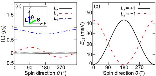
Figure S4: (a) Orbital polarization of an Fe ion in FePS₃ as a function of the direction of its spin polarization. Here, $\theta$ is the angle from $z$ (the out-of-plane direction of an FePS₃ monolayer) of the spin polairzation direction. (b) Magnetic anisotropy energy per Fe ion as a function of the spin polarization direction. The solid black curve and the dashed red curve represent the case of an Fe ion with $L_{z}\approx 1$ and that of an Fe ion with $L_{z}\approx-1$, respectively. The dash-dotted blue curve, which is slightly shifted downward for visual clarity, shows the lowest-energy at a given spin polarization direction.

Appendix D Isotropic interlayer exchange interactions

Table S1 shows the isotropic interlayer exchange interaction $K_{n}$ (= $1/3\,{\rm Tr}\,\mathbf{K}_{n}$) obtained from our calculations. For all TMPS₃’s the second-nearest-neighbor isotropic interlayer exchange interactions ($K_{3,4}$) are relatively large compared to the other $K_{n}$’s. Particularly in the case of NiPS₃, $K_{3,4}$ are 1.64 meV and as large as 30 % of $J_{1}^{(1\text{--}3)}$, indicating strong influence of the thickness on the magnetic properties of this compound. It is noteworthy that superexchange paths for $K_{n}$’s need to go through at least two S ions, e. g. , like TM-S-S-TM, and that such pathways are similar in their total length for all $K_{n}$’s considered in this work. This similarity partly explains how $K_{3,4}$ can be comparable to or even larger than the nearest-neighbor interlayer exchange interactions ($K_{1,2}$). Further investigation on the exchange mechanism behind $K_{n}$’s, which is beyond our current scope, would be helpful to address this issue, and we leave it for future studies.

	$K_{1}$	$K_{2}$	$K_{3}$	$K_{4}$	$K_{5}$	$K_{6}$	$K_{7}$	$K_{8}$
MnPS3	0.01	0.01	0.03	0.03	0.01	0.01	0.01	0.02
FePS3	0.04	0.04	0.11	0.12	0.03	0.03	0.03	0.05
NiPS3	$-$0.05	$-$0.08	1.64	1.64	0.47	0.36	0.36	0.46

Table S1: Isotropic interlayer exchange interaction $K_{n}$ in units of meV.

Appendix E Calculations details: classical Monte Carlo simulation

In our classical Monte Carlo simulations, the Metropolis algorithm [61] and a variant of the Wolff cluster algorithm [62], modified for inclusion of the anisotropic exchange interactions [63] and the single-ion anisotropy [64], were used to update spins during simulations. For each measurement, one Metropolis sweep of the entire spin lattice and 10 Wolff cluster updates were done. Typically, $10^{4}$–$10^{5}$ measurements were done for calculating thermodynamic quantities at a given temperature. The initial 20–50% of those measurements were discarded for thermalization. In the case of bulk TMPS₃, periodic boundary conditions were imposed for all the crystallographic directions ($\mathbf{a}$, $\mathbf{b}^{\prime}$, and $\mathbf{c}$ in Figure S2). We found that a superlattice containing $128\times 128\times 8$ unit cells including $128\times 128\times 8\times 2=4096$ spins was sufficient to converge the results. In the case of few-layer TMPS₃, periodic boundary conditions were used for only the in-plane directions ($\mathbf{a}$ and $\mathbf{b}^{\prime}$ in Figure S2). A $128\times 128\times 1$ superlattice was employed for the few-layer cases.

The magnetic susceptibility $\chi_{\mu}$ and the specific heat arising from the localized magnetic moments $c_{v}^{\rm mag}$ are defined as

$$\chi_{\mu}=\frac{\langle M_{\mu}^{2}\rangle-\langle M_{\mu}\rangle^{2}}{NT}$$ (E16)

and

$$c_{v}^{\rm mag}=\frac{\langle H^{2}_{\text{tot}}\rangle-\langle H_{\text{tot}}\rangle^{2}}{NT^{2}},$$ (E17)

respectively, where $\mu$ denotes the Cartesian direction $x$, $y$, and $z$, $N$ is the number of magnetic atoms, $T$ is the temperature, and $M_{\mu}$ is the total magnetic moment. The expression $\left<O\right>$ denotes the thermal average of a quantity $O$, i.e. the average of $O$ with the Boltzmann weight factor. In the case of MnPS₃ and NiPS₃, where the orbital degrees of freedom are suppressed ($L_{iz}=0$) by the crystal field effects, $\left<O\right>$ is simply a weighted average of $O[\{\mathbf{S}_{i}\}]$ over all spin configuration $\{\mathbf{S}_{i}\}$’s. It is straightforward to calculate this kind of weighted averages by using the importance sampling method, which is inherent in the process of updating spins by the algorithms we employed. If additional degrees of freedom arising from the orbital polarization should be considered, as in the case of FePS₃, things become much more complicated because then $\left<O\right>$ involves averaging over all possible orbital configurations, $\{L_{iz}\}$’s, as well as $\{\mathbf{S}_{i}\}$’s. In Section F, we discuss how to resolve this issue in practice.

Appendix F Orbital contributions to the magnetic susceptibility and specific heat

We present a detailed description of how the effects of the orbital degrees of freedom on thermodynamic quantities were treated in our Monte Carlo simulations. The basic idea is to integrate out orbital degrees of freedom in advance of averaging over spin degrees of freedom. We first consider the partition function $Z$ of the anisotropic magnetic model $H_{\rm tot}$ (eq A10):

$$Z=\sum_{\{\mathbf{S}_{i}\}}\sum_{\{L_{iz}\}}\left\{\exp\left[-\beta\left(H_{S{\rm only}}+\sum_{i=1}^{N}{\lambda L_{iz}S_{iz}}\right)\right]\right\},$$ (F18)

where $\beta$ is the inverse temperature $(k_{\text{B}}T)^{-1}$ and $H_{S{\rm only}}$ is the spin-only-dependent part of $H_{\rm tot}$ which reads

$$H_{S{\rm only}} =\frac{1}{2}\sum_{i=1}^{N}\sum_{n=1}^{3}\sum_{a=1}^{M_{n}}{\mathbf{S}_{i}^{\mathsf{T}}\,\mathbf{J}_{n}^{(a)}\,\mathbf{S}_{j(i,\mathbf{J}_{n}^{(a)})}}+\frac{1}{2}\sum_{i=1}^{N}\sum_{n=1}^{8}{\mathbf{S}_{i}^{\mathsf{T}}\,\mathbf{K}_{n}\,\mathbf{S}_{j(i,\mathbf{K}_{n})}}$$

$$+\sum_{i=1}^{N}{\mathbf{S}_{i}^{\mathsf{T}}\,\mathbf{D}\,\mathbf{S}_{i}}+H_{\text{dip}}.$$ (F19)

The summation over $\{L_{iz}\}$ in eq F18 can be done readily by exploiting that $L_{iz}$ can be either 1 or $-$1:

$$Z =\sum_{\{\mathbf{S}_{i}\}}\left\{\exp(-\beta H_{S{\rm only}})\sum_{\{L_{iz}\}}\left[\prod_{i=1}^{N}\exp\left(-\beta\lambda L_{iz}S_{iz}\right)\right]\right\}$$

$$=\sum_{\{\mathbf{S}_{i}\}}\left\{\exp(-\beta H_{S{\rm only}})\prod_{i=1}^{N}\left[\sum_{L_{iz}=\pm 1}\exp\left(-\beta\lambda L_{iz}S_{iz}\right)\right]\right\}$$

$$=\sum_{\{\mathbf{S}_{i}\}}\left\{\exp(-\beta H_{S{\rm only}})\prod_{i=1}^{N}2\cosh\left(-\beta\lambda S_{iz}\right)\right\}$$

$$=\sum_{\{\mathbf{S}_{i}\}}\left\{\exp\left[-\beta\left(H_{S{\rm only}}+\sum_{i=1}^{N}V_{i}(\beta,\lambda)\right)\right]\right\},$$ (F20)

where $V_{i}(\beta,\lambda)=-\beta^{-1}\ln\left[2\cosh\left(-\beta\lambda S_{iz}\right)\right]$. Here, $V_{i}(\beta,\lambda)$ can be thought of as an effective on-site potential that accounts for the effects of orbital degrees of freedom at a given temperature $T$.

The $z$ component of the total magnetic moment $\left<M_{z}\right>=\mu_{\rm B}\left<L_{z}+2S_{z}\right>$, where $L_{z}=\sum_{i=1}^{N}L_{iz}$ and $S_{z}=\sum_{i=1}^{N}S_{iz}$. The spin part can be written as

$$\left<S_{z}\right> =Z^{-1}\sum_{\{\mathbf{S}_{i}\}}\sum_{\{L_{iz}\}}\left\{S_{z}\exp\left[-\beta\left(H_{S{\rm only}}+\sum_{i=1}^{N}\lambda L_{iz}S_{iz}\right)\right]\right\}$$

$$=Z^{-1}\sum_{\{\mathbf{S}_{i}\}}\left\{S_{z}\exp(-\beta H_{S{\rm only}})\sum_{\{L_{iz}\}}\left[\prod_{i=1}^{N}\exp\left(-\beta\lambda L_{iz}S_{iz}\right)\right]\right\}$$

$$=Z^{-1}\sum_{\{\mathbf{S}_{i}\}}\left[S_{z}\exp(-\beta H_{S{\rm only}})\prod_{i=1}^{N}2\cosh\left(-\beta\lambda S_{iz}\right)\right]$$

$$=Z^{-1}\sum_{\{\mathbf{S}_{i}\}}\left\{S_{z}\exp\left[-\beta\left(H_{S{\rm only}}+\sum_{i=1}^{N}V_{i}(\beta,\lambda)\right)\right]\right\}$$

$$=\left<S_{z}\right>_{S}.$$ (F21)

Here, the notation $\left<O\right>_{S}$ was used to emphasize that the average was taken over spin configuration $\{\mathbf{S}_{i}\}$’s only, with the weight factor $Z^{-1}\exp[-\beta(H_{S{\rm only}}+\sum_{i=1}^{N}V_{i}(\beta,\lambda)]$. The orbital part can be written as a sum over possible spin configurations as well, i.e.

$$\left<L_{z}\right> =Z^{-1}\sum_{\{\mathbf{S}_{i}\}}\sum_{\{L_{iz}\}}\left\{L_{z}\exp\left[-\beta\left(H_{S{\rm only}}+\sum_{i=1}^{N}\lambda L_{iz}S_{iz}\right)\right]\right\}$$

$$=Z^{-1}\sum_{\{\mathbf{S}_{i}\}}\left\{\exp(-\beta H_{S{\rm only}})\sum_{\{L_{iz}\}}\left[L_{z}\prod_{i=1}^{N}\exp(-\beta\lambda L_{iz}S_{iz})\right]\right\}$$

$$=Z^{-1}\sum_{\{\mathbf{S}_{i}\}}\left\{\exp(-\beta H_{S{\rm only}})\sum_{\{L_{iz}\}}\left[\sum_{j=1}^{N}L_{jz}\prod_{i=1}^{N}\exp(-\beta\lambda L_{iz}S_{iz})\right]\right\}$$

$$=Z^{-1}\sum_{\{\mathbf{S}_{i}\}}\left\{\exp(-\beta H_{S{\rm only}})\sum_{j=1}^{N}\left[2\sinh(-\beta\lambda S_{jz})\prod_{i=1,i{\neq}j}^{N}2\cosh(-\beta\lambda S_{iz})\right]\right\}$$

$$=Z^{-1}\sum_{\{\mathbf{S}_{i}\}}\left\{\exp(-\beta H_{S{\rm only}})\sum_{j=1}^{N}\left[l_{jz}\prod_{i=1}^{N}2\cosh(-\beta\lambda S_{iz})\right]\right\}$$

$$=Z^{-1}\sum_{\{\mathbf{S}_{i}\}}\left\{\left(\sum_{j=1}^{N}l_{jz}\right)\exp\left[-\beta\left(H_{S{\rm only}}+\sum_{i=1}^{N}V_{i}(-\beta\lambda S_{iz})\right)\right]\right\}$$

$$=Z^{-1}\sum_{\{\mathbf{S}_{i}\}}\left\{l_{z}\exp\left[-\beta\left(H_{S{\rm only}}+\sum_{i=1}^{N}V_{i}(\beta,\lambda)\right)\right]\right\}$$

$$=\left<l_{z}\right>_{S},$$ (F22)

where $l_{iz}=\tanh(-\beta\lambda S_{iz})$ and $l_{z}=\sum_{i=1}^{N}l_{iz}$.

Some higher-order moments, such as $\langle L_{z}^{2}\rangle$, $\langle S_{z}L_{z}\rangle$, and $\langle S_{z}^{2}L_{z}^{2}\rangle$, which are needed in calculating $\chi_{z}$ and $c_{v}^{\rm mag}$, are written as

$$\langle L_{z}^{2}\rangle =Z^{-1}\sum_{\{\mathbf{S}_{i}\}}\sum_{\{L_{iz}\}}\left\{L_{z}^{2}\exp\left[-\beta\left(H_{S{\rm only}}+\sum_{i=1}^{N}\lambda L_{iz}S_{iz}\right)\right]\right\}$$

$$=Z^{-1}\sum_{\{\mathbf{S}_{i}\}}\left\{\exp(-\beta H_{S{\rm only}})\sum_{\{L_{iz}\}}\left[L_{z}^{2}\prod_{i=1}^{N}\exp(-\beta\lambda L_{iz}S_{iz})\right]\right\}$$

$$=Z^{-1}\sum_{\{\mathbf{S}_{i}\}}\left\{\exp(-\beta H_{S{\rm only}})\sum_{\{L_{iz}\}}\left[\sum_{j=1}^{N}\sum_{k=1}^{N}L_{jz}L_{kz}\prod_{i=1}^{N}\exp(-\beta\lambda L_{iz}S_{iz})\right]\right\}$$

$$=Z^{-1}\sum_{\{\mathbf{S}_{i}\}}\left\{\exp(-\beta H_{S{\rm only}})\sum_{\{L_{iz}\}}\left[\sum_{j=1}^{N}\left(1+\sum_{k=1,k{\neq}j}^{N}L_{jz}L_{kz}\right)\prod_{i=1}^{N}\exp(-\beta\lambda L_{iz}S_{iz})\right]\right\}$$

$$=Z^{-1}\sum_{\{\mathbf{S}_{i}\}}\left\{\exp(-\beta H_{S{\rm only}})\sum_{j=1}^{N}\left[\left(1+\sum_{k=1,k{\neq}j}^{N}l_{jz}l_{kz}\right)\prod_{i=1}^{N}2\cosh(-\beta\lambda S_{iz})\right]\right\}$$

$$=Z^{-1}\sum_{\{\mathbf{S}_{i}\}}\left\{\exp(-\beta H_{S{\rm only}})\sum_{j=1}^{N}\left[\left(1-l_{jz}^{2}+\sum_{k=1}^{N}l_{jz}l_{kz}\right)\prod_{i=1}^{N}2\cosh(-\beta\lambda S_{iz})\right]\right\}$$

$$=Z^{-1}\sum_{\{\mathbf{S}_{i}\}}\left\{\left[l_{z}^{2}+\sum_{j=1}^{N}(1-l_{jz}^{2})\right]\exp\left[-\beta(H_{S{\rm only}}+\sum_{i=1}^{N}V_{i}(\beta,\lambda)\right]\right\}$$

$$=\left<l_{z}^{2}+\sum_{i=1}^{N}(1-l_{iz}^{2})\right>_{S},$$ (F23)

$$\langle S_{z}L_{z}\rangle=\left<S_{z}l_{z}\right>_{S},$$ (F24)

and

$$\langle S_{z}^{2}L_{z}^{2}\rangle=\left<S_{z}^{2}\left\{l_{z}^{2}+\sum_{i=1}^{N}(1-l_{iz}^{2})\right\}\right>_{S},$$ (F25)

respectively.

Putting eqs F21–F25 into eqs E16 and E17, we obtain the expressions for $\chi_{z}$ and $c_{v}^{\rm mat}$:

$$\chi_{z}=\mu_{\rm B}^{2}\frac{\langle(l_{z}+2S_{z})^{2}\rangle_{S}-\langle l_{z}+2S_{z}\rangle_{S}^{2}+\langle\sum_{i=1}^{N}(1-l_{iz}^{2})\rangle_{S}}{NT}.$$ (F26)

and

$$c_{v}^{\text{mag}}=\frac{\langle H_{\rm tot,eff}^{2}\rangle_{S}-\langle H_{\rm tot,eff}\rangle_{S}^{2}+\langle\lambda^{2}\sum_{i=1}^{N}(1-l_{iz}^{2})S_{iz}^{2}\rangle_{S}}{NT^{2}},$$ (F27)

respectively, where $H_{\rm tot,eff}=H_{S{\rm only}}+\sum_{i=1}^{N}\lambda l_{iz}S_{iz}$.

Appendix G Quantum fluctuation effects on the stability of the antiferromagnetic ground state of monolayer NiPS₃

The isotropic intralayer exchange interactions ($J_{n}^{(a)}$, up to 28 meV) are much larger in magnitude than other constituents of our magnetic Hamiltonian for NiPS₃: the anisotropic intralayer exchange interactions (the traceless part of $\mathbf{J}_{n}^{(a)}$, $\sim$0.07 meV), the single-ion anisotropy ($\mathbf{D}$, $\sim$0.1 meV), and the dipolar anisotropy energy ($\sim$0.025 meV per transition metal ion). Therefore, we consider the quantum fluctuation effects in the $J_{1}$-$J_{2}$-$J_{3}$ Heisenberg model to gain insight into the possibility of a quantum spin liquid phase in monolayer NiPS₃.

Because $S$=1 for the Ni²⁺ ions ($3d^{8}$, high-spin configuration), the quantum effects of $S$=1 are of our particular interest. According to a study on the quantum ($S$=1/2 and $S$=1) $J_{1}$-$J_{2}$-$J_{3}$ model on the honeycomb lattice [65], the quantum spin liquid phase, which exists in a very small region in the parameter space in the case of $S$=1/2 (by the way, the sets of parameters for all three TMPS₃ compounds are outside this small region), disappears in the case of $S$=1 due to the weakening of quantum fluctuations. A spin liquid phase driven by the frustration arising from competing $J_{1}$, $J_{2}$, and $J_{3}$ is therefore not likely to happen.

In addition to the suppression of the quantum spin liquid phase, the phase boundaries of the classical $J_{1}$-$J_{2}$-$J_{3}$ model on the honeycomb lattice (see Figure S5) is only slightly changed when the quantum effects of $S$=1 are taken into account [65]. Since our magnetic model for NiPS₃ is well-separated from any of those phase boundaries (see Figure S5b), the stability of the zigzag antiferromagnetic phase, which is the low temperature phase of monolayer NiPS₃ given by the classical $J_{1}$-$J_{2}$-$J_{3}$ model, would not be affected by such small quantum fluctuation effects.

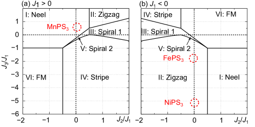
Figure S5: Phase diagrams of the classical $J_{1}$-$J_{2}$-$J_{3}$ model on the honeycomb lattice for (a) $J_{1}>0$ for MnPS₃ and (b) $J_{1}<0$ for FePS₃ and NiPS₃ (adapted from ref 66).

For all these reasons, for monolayer NiPS₃, the classical $J_{1}$-$J_{2}$-$J_{3}$ model provides almost the same answer as the quantum ($S$=1) $J_{1}$-$J_{2}$-$J_{3}$ model. Our use of classical Monte Carlo simulation can be justified in this regard.

Because the magnitude of the isotropic intralayer exchange interaction is much larger than that of the other contributions (the anisotropic intralayer exchange interactions, the single-ion anisotropy, and the dipolar anisotropy), we expect that our conclusion given above will not change when those minor contributions are fully considered within the quantum version ($S$=1) of our magnetic model for NiPS₃.

References

- Gong et al. [2017] C. Gong, L. Li, Z. Li, H. Ji, A. Stern, Y. Xia, T. Cao, W. Bao, C. Wang, Y. Wang, Z. Q. Qiu, R. J. Cava, S. G. Louie, J. Xia, and X. Zhang, Discovery of intrinsic ferromagnetism in two-dimensional van der Waals crystals, Nature 546, 265 (2017).
- Huang et al. [2017] B. Huang, G. Clark, E. Navarro-Moratalla, D. R. Klein, R. Cheng, K. L. Seyler, D. Zhong, E. Schmidgall, M. A. McGuire, D. H. Cobden, W. Yao, D. Xiao, P. Jarillo-Herrero, and X. Xu, Layer-dependent ferromagnetism in a van der Waals crystal down to the monolayer limit, Nature 546, 270 (2017).
- Lee et al. [2016a] S. Lee, K.-Y. Choi, S. Lee, B. H. Park, and J.-G. Park, Tunneling transport of mono- and few-layers magnetic van der Waals MnPS3, APL Mater. 4, 086108 (2016a).
- Du et al. [2016] K.-z. Du, X.-z. Wang, Y. Liu, P. Hu, M. I. B. Utama, C. K. Gan, Q. Xiong, and C. Kloc, Weak van der waals stacking, wide-range band gap, and raman study on ultrathin layers of metal phosphorus trichalcogenides, ACS Nano 10, 1738 (2016).
- Kuo et al. [2016] C.-T. Kuo, M. Neumann, K. Balamurugan, H. J. Park, S. Kang, H. W. Shiu, J. H. Kang, B. H. Hong, M. Han, T. W. Noh, and J.-G. Park, Exfoliation and Raman Spectroscopic Fingerprint of Few-Layer NiPS3 Van der Waals Crystals, Sci. Rep. 6, 20904 (2016).
- Lee et al. [2016b] J.-U. Lee, S. Lee, J. H. Ryoo, S. Kang, T. Y. Kim, P. Kim, C.-H. Park, J.-G. Park, and H. Cheong, Ising-type magnetic ordering in atomically thin FePS3, Nano Lett. 16, 7433 (2016b).
- Kim et al. [2019a] K. Kim, S. Y. Lim, J.-U. Lee, S. Lee, T. Y. Kim, K. Park, G. S. Jeon, C.-H. Park, J.-G. Park, and H. Cheong, Suppression of magnetic ordering in XXZ-type antiferromagnetic monolayer NiPS3, Nat. Commun. 10, 345 (2019a).
- Kim et al. [2019b] K. Kim, S. Y. Lim, J. Kim, J.-U. Lee, S. Lee, P. Kim, K. Park, S. Son, C.-H. Park, J.-G. Park, and H. Cheong, Antiferromagnetic ordering in van der Waals 2D magnetic material MnPS3 probed by Raman spectroscopy, 2D Mater. 6, 041001 (2019b).
- Lim et al. [2021] S. Y. Lim, K. Kim, S. Lee, J.-G. Park, and H. Cheong, Thickness dependence of antiferromagnetic phase transition in Heisenberg-type MnPS3, Curr. Appl. Phys. 21, 1 (2021).
- Kang et al. [2020] S. Kang, K. Kim, B. H. Kim, J. Kim, K. I. Sim, J.-U. Lee, S. Lee, K. Park, S. Yun, T. Kim, A. Nag, A. Walters, M. Garcia-Fernandez, J. Li, L. Chapon, K.-J. Zhou, Y.-W. Son, J. H. Kim, H. Cheong, and J.-G. Park, Coherent many-body exciton in van der Waals antiferromagnet NiPS3, Nature 583, 785 (2020).
- Hwangbo et al. [2021] K. Hwangbo, Q. Zhang, Q. Jiang, Y. Wang, J. Fonseca, C. Wang, G. M. Diederich, D. R. Gamelin, D. Xiao, J.-H. Chu, W. Yao, and X. Xu, Highly anisotropic excitons and multiple phonon bound states in a van der Waals antiferromagnetic insulator, Nat. Nanotechnol. 16, 655 (2021).
- Zhang et al. [2021] Q. Zhang, K. Hwangbo, C. Wang, Q. Jiang, J.-H. Chu, H. Wen, D. Xiao, and X. Xu, Observation of giant optical linear dichroism in a zigzag antiferromagnet FePS3, Nano Lett. 21, 6938 (2021).
- Mermin and Wagner [1966] N. D. Mermin and H. Wagner, Absence of ferromagnetism or antiferromagnetism in one- or two-dimensional isotropic heisenberg models, Phys. Rev. Lett. 17, 1133 (1966).
- Berezinskiǐ [1972] V. L. Berezinskiǐ, Destruction of long-range order in one-dimensional and two-dimensional systems possessing a continuous symmetry group. II. Quantum systems, Soviet Journal of Experimental and Theoretical Physics 34, 610 (1972).
- Kosterlitz and Thouless [1973] J. M. Kosterlitz and D. J. Thouless, Ordering, metastability and phase transitions in two-dimensional systems, J. Phys. C: Solid State Phys. 6, 1181 (1973).
- Joy and Vasudevan [1992] P. A. Joy and S. Vasudevan, Magnetism in the layered transition-metal thiophosphates MPS3 (M=Mn, Fe, and Ni), Phys. Rev. B 46, 5425 (1992).
- Vaclavkova et al. [2020] D. Vaclavkova, A. Delhomme, C. Faugeras, M. Potemski, A. Bogucki, J. Suffczyński, P. Kossacki, A. R. Wildes, B. Grémaud, and A. Saúl, Magnetoelastic interaction in the two-dimensional magnetic material MnPS3 studied by first principles calculations and Raman experiments, 2D Mater. 7, 035030 (2020).
- Olsen [2021] T. Olsen, Magnetic anisotropy and exchange interactions of two-dimensional FePS3, NiPS3 and MnPS3 from first principles calculations, Journal of Physics D: Applied Physics 54, 314001 (2021).
- Bacaksiz et al. [2021] C. Bacaksiz, D. Šabani, R. M. Menezes, and M. V. Milošević, Distinctive magnetic properties of CrI3 and CrBr3 monolayers caused by spin-orbit coupling, Phys. Rev. B 103, 125418 (2021).
- Nauman et al. [2021] M. Nauman, D. H. Kiem, S. Lee, S. Son, J.-G. Park, W. Kang, M. J. Han, and Y. Jo, Complete mapping of magnetic anisotropy for prototype Ising van der Waals FePS3, 2D Mater. 8, 035011 (2021).
- Brec [1986] R. Brec, Review on structural and chemical properties of transition metal phosphorus trisulfides MPS3, in Intercalation in Layered Materials, edited by M. S. Dresselhaus (Springer US, Boston, MA, 1986) pp. 93–124.
- Lançon et al. [2018] D. Lançon, R. A. Ewings, T. Guidi, F. Formisano, and A. R. Wildes, Magnetic exchange parameters and anisotropy of the quasi-two-dimensional antiferromagnet NiPS3, Phys. Rev. B 98, 134414 (2018).
- Pellegrini et al. [2020] C. Pellegrini, T. Müller, J. K. Dewhurst, S. Sharma, A. Sanna, and E. K. U. Gross, Density functional theory of magnetic dipolar interactions, Phys. Rev. B 101, 144401 (2020).
- Kurosawa et al. [1983] K. Kurosawa, S. Saito, and Y. Yamaguchi, Neutron diffraction study on MnPS3 and FePS3, Journal of the Physical Society of Japan 52, 3919 (1983).
- Lançon et al. [2016] D. Lançon, H. C. Walker, E. Ressouche, B. Ouladdiaf, K. C. Rule, G. J. McIntyre, T. J. Hicks, H. M. Rønnow, and A. R. Wildes, Magnetic structure and magnon dynamics of the quasi-two-dimensional antiferromagnet FePS3, Phys. Rev. B 94, 214407 (2016).
- Wildes et al. [2015] A. R. Wildes, V. Simonet, E. Ressouche, G. J. McIntyre, M. Avdeev, E. Suard, S. A. J. Kimber, D. Lançon, G. Pepe, B. Moubaraki, and T. J. Hicks, Magnetic structure of the quasi-two-dimensional antiferromagnet NiPS3, Phys. Rev. B 92, 224408 (2015).
- Lane and Zhu [2020] C. Lane and J.-X. Zhu, Thickness dependence of electronic structure and optical properties of a correlated van der Waals antiferromagnetic NiPS3 thin film, Phys. Rev. B 102, 075124 (2020).
- Takano et al. [2004] Y. Takano, N. Arai, A. Arai, Y. Takahashi, K. Takase, and K. Sekizawa, Magnetic properties and specific heat of MPS3 (M=Mn, Fe, Zn), J. Magn. Magn. Mater. Proceedings of the International Conference on Magnetism (ICM 2003), 272–276, E593 (2004).
- Šiškins et al. [2019] M. Šiškins, M. Lee, S. Mañas-Valero, E. Coronado, Y. M. Blanter, H. S. J. van der Zant, and P. G. Steeneken, Magnetic and electronic phase transitions probed by nanomechanical resonance, arXiv:1911.08537 [cond-mat, physics:physics] (2019).
- Wildes et al. [2007] A. R. Wildes, H. M. Rønnow, B. Roessli, M. J. Harris, and K. W. Godfrey, Anisotropy and the critical behaviour of the quasi-2D antiferromagnet, MnPS3, J. Magn. Magn. Mater. Proceedings of the 17th International Conference on Magnetism, 310, 1221 (2007).
- Hicks et al. [2019] T. J. Hicks, T. Keller, and A. R. Wildes, Magnetic dipole splitting of magnon bands in a two dimensional antiferromagnet, J. Magn. Magn. Mater. 474, 512 (2019).
- Torelli et al. [2019] D. Torelli, K. S. Thygesen, and T. Olsen, High throughput computational screening for 2D ferromagnetic materials: The critical role of anisotropy and local correlations, 2D Mater. 6, 045018 (2019).
- Olsen [2019] T. Olsen, Theory and simulations of critical temperatures in CrI3 and other 2D materials: Easy-axis magnetic order and easy-plane Kosterlitz–Thouless transitions, MRS Communications 9, 1142 (2019).
- Chittari et al. [2016] B. L. Chittari, Y. Park, D. Lee, M. Han, A. H. MacDonald, E. Hwang, and J. Jung, Electronic and magnetic properties of single-layer MPX3 metal phosphorous trichalcogenides, Phys. Rev. B 94, 184428 (2016).
- Sears et al. [2017] J. A. Sears, Y. Zhao, Z. Xu, J. W. Lynn, and Y.-J. Kim, Phase diagram of -RuCl3 in an in-plane magnetic field, Phys. Rev. B 95, 180411(R) (2017).
- Wong et al. [2019] P. K. J. Wong, W. Zhang, F. Bussolotti, X. Yin, T. S. Herng, L. Zhang, Y. L. Huang, G. Vinai, S. Krishnamurthi, D. W. Bukhvalov, Y. J. Zheng, R. Chua, A. T. N’Diaye, S. A. Morton, C.-Y. Yang, K.-H. Ou Yang, P. Torelli, W. Chen, K. E. J. Goh, J. Ding, M.-T. Lin, G. Brocks, M. P. de Jong, A. H. Castro Neto, and A. T. S. Wee, Evidence of spin frustration in a vanadium diselenide monolayer magnet, Adv. Matter. 31, 1901185 (2019).
- Giannozzi et al. [2009] P. Giannozzi, S. Baroni, N. Bonini, M. Calandra, R. Car, C. Cavazzoni, D. Ceresoli, G. L. Chiarotti, M. Cococcioni, I. Dabo, A. D. Corso, S. de Gironcoli, S. Fabris, G. Fratesi, R. Gebauer, U. Gerstmann, C. Gougoussis, A. Kokalj, M. Lazzeri, L. Martin-Samos, N. Marzari, F. Mauri, R. Mazzarello, S. Paolini, A. Pasquarello, L. Paulatto, C. Sbraccia, S. Scandolo, G. Sclauzero, A. P. Seitsonen, A. Smogunov, P. Umari, and R. M. Wentzcovitch, QUANTUM ESPRESSO: A modular and open-source software project for quantum simulations of materials, J. Phys.: Condens. Matter 21, 395502 (2009).
- Ma and Dudarev [2015] P.-W. Ma and S. L. Dudarev, Constrained density functional for noncollinear magnetism, Phys. Rev. B 91, 054420 (2015).
- Perdew and Zunger [1981] J. P. Perdew and A. Zunger, Self-interaction correction to density-functional approximations for many-electron systems, Phys. Rev. B 23, 5048 (1981).
- Liechtenstein et al. [1995] A. I. Liechtenstein, V. I. Anisimov, and J. Zaanen, Density-functional theory and strong interactions: Orbital ordering in Mott-Hubbard insulators, Phys. Rev. B 52, R5467 (1995).
- Timrov et al. [2018] I. Timrov, N. Marzari, and M. Cococcioni, Hubbard parameters from density-functional perturbation theory, Phys. Rev. B 98, 085127 (2018).
- Aryasetiawan et al. [2006] F. Aryasetiawan, K. Karlsson, O. Jepsen, and U. Schönberger, Calculations of Hubbard U from first-principles, Phys. Rev. B 74, 125106 (2006).
- Hamann [2013] D. R. Hamann, Optimized norm-conserving Vanderbilt pseudopotentials, Phys. Rev. B 88, 085117 (2013).
- Schlipf and Gygi [2015] M. Schlipf and F. Gygi, Optimization algorithm for the generation of ONCV pseudopotentials, Comput. Phys. Commun. 196, 36 (2015).
- Ouvrard et al. [1985] G. Ouvrard, R. Brec, and J. Rouxel, Structural determination of some MPS3 layered phases (M = Mn, Fe, Co, Ni and Cd), Mater. Res. Bull. 20, 1181 (1985).
- Solovyev et al. [2015] I. V. Solovyev, V. V. Mazurenko, and A. A. Katanin, Validity and limitations of the superexchange model for the magnetic properties of Sr2IrO4 and Ba2IrO4 mediated by the strong spin-orbit coupling, Phys. Rev. B 92, 235109 (2015).
- Fang and Nagaosa [2004] Z. Fang and N. Nagaosa, Quantum versus jahn-teller orbital physics in YVO3 and LaVO3, Phys. Rev. Lett. 93, 176404 (2004).
- Yaresko et al. [2009] A. N. Yaresko, G.-Q. Liu, V. N. Antonov, and O. K. Andersen, Interplay between magnetic properties and Fermi surface nesting in iron pnictides, Phys. Rev. B 79, 144421 (2009).
- Jacobsson et al. [2013] A. Jacobsson, B. Sanyal, M. Ležaić, and S. Blügel, Exchange parameters and adiabatic magnon energies from spin-spiral calculations, Phys. Rev. B 88, 134427 (2013).
- Foyevtsova et al. [2013] K. Foyevtsova, H. O. Jeschke, I. I. Mazin, D. I. Khomskii, and R. Valentí, Ab initio analysis of the tight-binding parameters and magnetic interactions in Na2IrO3, Phys. Rev. B 88, 035107 (2013).
- Lambrecht et al. [2003] W. R. L. Lambrecht, M. Prikhodko, and M. S. Miao, Electronic structure and magnetic interactions in MnN and Mn3N2, Phys. Rev. B 68, 174411 (2003).
- Monkhorst and Pack [1976] H. J. Monkhorst and J. D. Pack, Special points for Brillouin-zone integrations, Phys. Rev. B 13, 5188 (1976).
- Hobbs et al. [2000] D. Hobbs, G. Kresse, and J. Hafner, Fully unconstrained noncollinear magnetism within the projector augmented-wave method, Phys. Rev. B 62, 11556 (2000).
- Scalmani and Frisch [2012] G. Scalmani and M. J. Frisch, A New Approach to Noncollinear Spin Density Functional Theory beyond the Local Density Approximation, J. Chem. Theory Comput. 8, 2193 (2012).
- [55] The elk code (https://elk.sourceforge.io).
- Kresse and Furthmüller [1996] G. Kresse and J. Furthmüller, Efficient iterative schemes for ab initio total-energy calculations using a plane-wave basis set, Phys. Rev. B 54, 11169 (1996).
- Eich et al. [2013] F. G. Eich, S. Pittalis, and G. Vignale, Transverse and longitudinal gradients of the spin magnetization in spin-density-functional theory, Phys. Rev. B 88, 245102 (2013).
- Desmarais et al. [2019] J. K. Desmarais, J.-P. Flament, and A. Erba, Spin-orbit coupling from a two-component self-consistent approach. I. Generalized Hartree-Fock theory, J. Chem. Phys. 151, 074107 (2019).
- Desmarais et al. [2021] J. K. Desmarais, J.-P. Flament, and A. Erba, Retraction: “Spin-orbit coupling from a two-component self-consistent approach. II. Non-collinear density functional theories” [J. Chem. Phys. 151, 074108 (2019)], J. Chem. Phys. 154, 159901 (2021).
- Liechtenstein et al. [1987] A. I. Liechtenstein, M. I. Katsnelson, V. P. Antropov, and V. A. Gubanov, Local spin density functional approach to the theory of exchange interactions in ferromagnetic metals and alloys, J. Magn. Magn. Mater. 67, 65 (1987).
- Metropolis et al. [1953] N. Metropolis, A. W. Rosenbluth, M. N. Rosenbluth, A. H. Teller, and E. Teller, Equation of State Calculations by Fast Computing Machines, J. Chem. Phys. 21, 1087 (1953).
- Wolff [1989] U. Wolff, Collective monte carlo updating for spin systems, Phys. Rev. Lett. 62, 361 (1989).
- D’Onorio De Meo and Oh [1992] M. D’Onorio De Meo and S. K. Oh, Wolff algorithm and anisotropic continuous-spin models: An application to the spin–van der Waals model, Phys. Rev. B 46, 257 (1992).
- Leblanc et al. [2013] M. D. Leblanc, J. P. Whitehead, and M. L. Plumer, Monte Carlo simulations of intragrain spin effects in a quasi-2D Heisenberg model with uniaxial anisotropy, J. Phys.: Condens. Matter 25, 196004 (2013).
- Merino and Ralko [2018] J. Merino and A. Ralko, Role of quantum fluctuations on spin liquids and ordered phases in the Heisenberg model on the honeycomb lattice, Phys. Rev. B 97, 205112 (2018).
- Fouet et al. [2001] J. Fouet, P. Sindzingre, and C. Lhuillier, An investigation of the quantum J1-J2-J3 model on the honeycomb lattice, Eur. Phys. J. B 20, 241 (2001).