Gravitational Microlensing Rates in Milky Way Globular Clusters

Abstract

Many recent observational and theoretical studies suggest that globular clusters (GCs) host compact object populations large enough to play dominant roles in their overall dynamical evolution. Yet direct detection, particularly of black holes and neutron stars, remains rare and limited to special cases, such as when these objects reside in close binaries with bright companions. Here we examine the potential of microlensing detections to further constrain these dark populations. Based on state-of-the-art GC models from the CMC Cluster Catalog, we estimate the microlensing event rates for black holes, neutron stars, white dwarfs, and, for comparison, also for M dwarfs in Milky Way GCs, as well as the effects of different initial conditions on these rates. Among compact objects, we find that white dwarfs dominate the microlensing rates, simply because they largely dominate by numbers. We show that microlensing detections are in general more likely in GCs with higher initial densities, especially in clusters that undergo core collapse. We also estimate microlensing rates in the specific cases of M22 and 47 Tuc using our best-fitting models for these GCs. Because their positions on the sky lie near the rich stellar backgrounds of the Galactic bulge and the Small Magellanic Cloud, respectively, these clusters are among the Galactic GCs best-suited for dedicated microlensing surveys. The upcoming 10-year survey with the Rubin Observatory may be ideal for detecting lensing events in GCs.

1 Introduction

Constraining the demographics of compact object populations in globular clusters (GCs) has been of high interest in astronomy for several decades. Compact objects—stellar-mass black holes (BHs), neutron stars (NSs), and white dwarfs (WDs)—are the key ingredients for a wide array of sources and phenomena observed in clusters, including X-ray binaries (Katz_1975; Clark_1975; Verbunt_1984; Heinke_2005; Ivanova_2013; Giesler_2018; Kremer_2018a), millisecond radio pulsars (Lyne_1987; Sigurdsson_1995; Camilo_2005; Ransom_2008; Chomiuk_2013; Shishkovsky_2018; Fragione_2018c; Ye_2019), fast radio bursts (Kirsten_2021; Kremer_2021_FRB), and gravitational wave events (Moody_2008; Banerjee_2010; Bae_2014; Ziosi_2014; Rodriguez_2015; Rodriguez_2016; Askar_2016; Banerjee_2017; Hong_2018; Fragione_2018; Samsing_2018; Rodriguez_2018; Zevin_2019; Kremer_2019d). Populations of compact objects also greatly impact the overall dynamical evolution of GCs; in particular, stellar BHs can quickly concentrate in the cluster core due to dynamical friction and subsequently heat the cluster through frequent binary-mediated encounters (Spitzer_1969; Heggie_2003; Breen_2013; Kremer_2019b). Furthermore, massive WDs can dominate the central regions of core-collapsed GCs, also driving their dynamical evolution (e.g., Kremer_2020; Rui_2021b; Kremer_2021).

Observations and theory alike strongly indicate the existence of compact object populations in GCs. Milky Way GCs contain several known stellar-mass BH binary candidates detected via radio and X-ray observations, including in NGC 4472 (Maccarone_2007), M22 (Strader_2012), M62 (Chomiuk_2013), 47 Tuc (Miller-Jones_2015), and M10 (Shishkovsky_2018), as well as those detected via radial velocity measurements in NGC 3201 (Giesers_2018; Giesers_2019). Numerical simulations of GCs reinforce this observational evidence by demonstrating that Milky Way GCs can retain large populations of stellar-mass BHs up to the present day (e.g., Merritt_2004; Mackey_2007; Mackey_2008; Breen_2013; Morscher_2015; Peuten_2016; Chatterjee_2017a; Chatterjee_2017b; Askar_2018; Kremer_2018b; Kremer_2020; Weatherford_2018; Weatherford_2020; Antonini_2020). Meanwhile, observations of millisecond pulsars and low-mass X-ray binaries with neutron star accretors suggest that Milky Way GCs may on average contain hundreds of NSs each (e.g., Ivanova_2008; Kuranov_2006). Observations of WDs in GCs are also important; notably they enable stronger predictions of their host clusters’ ages (Hansen_2002; Hansen_2007; Hansen_2013) and distances (Renzini_1996). WDs are also observable as cataclysmic variables via their variability, emission lines, colours and X-ray emission (i.e., Knigge_2012). However, with their relatively large distances, GC cataclysmic variables are 10-100 times less bright than nearby ones observed in the Galactic field.

Yet the aforementioned observations are largely limited to special cases, particularly for BHs. Although NSs are detectable as pulsars and the younger, luminous end of the WD sequence is observable in some nearby clusters (e.g., Richer_1995; Richer_1997; Cool_1996), compact objects in GCs have otherwise only been directly detected in binaries via their influence on a luminous companion. This can be problematic when trying to use existing observations to constrain bulk properties of compact object populations in GCs. For example, dynamical simulations of GCs establish that the number of cluster BHs residing in binaries with luminous companions does not correlate with the total number of BHs in a cluster (Chatterjee_2017b; Kremer_2018a). The apparent BH mass distribution in clusters—useful for constraining supernova and collision physics as well as the cluster initial mass function and star formation history—is susceptible to bias if based solely on observations from binaries. In particular, mass segregation tends to cause the most massive BHs to form binaries with other BHs, not with observable stellar companions; the inferred BH mass distribution from observable BH binaries with a stellar companion could therefore be biased toward lower masses. Thus, in order to better constrain properties of the complete population of compact objects in clusters, additional observational strategies are necessary. Compact object detection through gravitational microlensing may serve such a purpose.

Because the fine alignment required to produce a microlensing event is rare and short-lived, searches for these events are challenging; for instance, early searches by the Massive Astrophysical Compact Halo Object (MACHO) collaboration revealed only three microlensing events by Galactic halo objects despite monitoring nearly $10^{7}$ stars in the Large Magellanic Cloud for over a year (Alcock_1995; Alcock_1996). Early efforts sought to constrain dark compact object populations in the mass range $10^{-7}<M/M_{\odot}<10^{-1}$ in the Galactic halo and bulge (e.g., Paczynski_1986; Paczynski_1991; Griest_1991; deRujula_1991). Since then, however, many microlensing events towards the Galactic bulge have been detected by several collaborations like the Optical Gravitational Lensing Experiment (OGLE; Udalski_1994; Udalski_2003; Udalski_2015), MACHO (Alcock_2000), and Microlensing Observations in Astrophysics (MOA; Bond_2001). Microlensing detections are accelerating as large surveys proliferate. In particular, the OGLE-IV survey now detects around 2000 photometric microlensing events towards the Galactic bulge every year (Udalski_2015). Most recently, Sahu_2022 reported the detection of the BH lensing event MOA-11-191/OGLE-11-0462 towards the Galactic Bulge with the BH inferred mass $\sim 7.1~{}M_{\odot}$. The same event has been analyzed in another recent work by Lam_2022 although they come to a slightly different conclusion than Sahu_2022 regarding the nature of the object. Thanks to such surveys, the future for microlensing is looking brighter.

The increasing frequency of microlensing detections has led to several recent theoretical studies of microlensing rates for compact objects, including stellar-mass BHs (Lu_2016; Zaris_2020), intermediate-mass BHs (Kains_2016; Safonova_2007; Kains_2018), NSs (Dai_2018), and WDs (McGill_2018). In particular, Harding_2017 estimate the microlensing event rate by nearby WD populations to be 30-50 per decade. Due to a small sample of BHs and NSs with well-known distances and proper motions, however, their estimates of the BH and NS rates are less certain.

In general, GCs have well-known distances and velocities, enabling more precise estimates of microlensing rates in these environments. GCs also feature dense populations of compact objects, making their optical depths much higher than in the field of the Milky Way. Paczynski_1994 originally proposed microlensing searches on GCs set against the backdrop of the dense Galactic bulge or the Small Magellanic Cloud. The first microlensing event in a GC was observed in M22 and the source star was located in the Galactic bulge (Pietrukowicz_2012). In addition to lensing of distant background stars, GCs can also produce observable microlensing events of the cluster stars themselves (so-called “self-lensing”). In this context, using the bright stars in NGC 5139 as sources, Zaris_2020 estimated the self-lensing rate of BHs in NGC 5139 to be in the range $0.1$–$1\,\rm{yr}^{-1}$ from their numerical simulations. While a reasonable number of self-lensing events in the dense regions of GCs can in principle occur for a large number of lenses ($\gtrsim 10^{4}$) and high velocity dispersion, detection requires high resolution imaging of the cluster background stars with powerful telescopes. Moreover, with fewer bright stars contained in GCs compared to the entire field of the Milky Way, many GCs would likely need to be observed to detect some microlensing events (Jetzer_1998).

In this paper, we analyse potential microlensing events in GCs using our realistic CMC Cluster Catalog models (Kremer_2020) with state-of-the-art prescriptions for the formation and kinematics of compact objects. In addition to predicting microlensing rates for compact objects, we also estimate the rates for M dwarfs, which usually dominate the cluster mass function in our models. In the rate analysis, we give additional attention to the clusters 47 Tuc (Ye_2021) and M22 (Kremer_2019a) given the higher potential for microlensing events provided by these clusters’ densely-populated backgrounds on the sky, i.e., the Small Magellanic Cloud (SMC) and the Galactic bulge, respectively.

This paper is structured as follows. In Section 2, we describe the computational method used to construct the CMC Cluster Catalog models, as well as the criteria we use to determine which additional CMC models most closely match 47 Tuc and M22. In Section 3, we review the basics of microlensing and explain how we estimate microlensing rates both numerically and analytically from our models. In Section 4, we present the microlensing rates due to sources both within the cluster (self-lensing) and outside the cluster (the distant background). Finally, in Section LABEL:sec:discussion, we summarize and discuss our results.

2 Modeling dense star clusters

2.1 CMC Catalog Models

In this paper, we predict gravitational lensing rates in the Milky Way GCs based on a large grid of cluster simulations recently published as the CMC Cluster Catalog (Kremer_2020). In particular, we analyse the microlensing event rates of 10 of the catalog’s 148 cluster simulations generated with our publicly released Cluster Monte Carlo (CMC) code (Rodriguez2021, and references therein). CMC is a Hénon-type Monte Carlo code (henon1971monte; henon1971montecluster) that has been continuously developed and improved for over two decades, beginning with Joshi_2000; Joshi_2001 and Fregeau_2003. The Monte Carlo Hénon method assumes spherical symmetry and orbit averaging, and is parallelized (Pattabiraman_2013), allowing us to model $10^{6}$ stars over a Hubble time in a couple days. CMC incorporates all relevant physical processes, such as two-body relaxation, three- and four-body strong encounters Fregeau_2007, three-body binary formation (Morscher_2015), and physical collisions and relativistic dynamics (Rodriguez_2018). It also includes stellar and binary evolution Hurley_2000; Hurley_2002 integrated with the COSMIC package for binary population synthesis Breivik_2020. We direct the reader to Rodriguez2021 for a detailed description of CMC’s implementation of all these processes, including up-to-date prescriptions for compact object formation.

All the catalog models adopt the standard Kroupa_2001 initial mass function (IMF) in the mass range 0.08-150$\,M_{\odot}$. The initial stellar velocities and positions of all objects draw from a King profile with initial central concentration $W_{0}=5$ King_1962. Our models do not include primordial mass segregation, so the initial velocities and positions of all objects do not depend on object mass. In this work, we explore the effect of the initial total number of objects $N$ and the initial cluster virial radius $r_{v}$ on the microlensing event rates while fixing other initial conditions such as the metallicity $Z=0.1\,Z_{\odot}$ and the Galactocentric radius $R_{\rm gc}=8$ kpc. Specifically, we use catalog models with initial $N=8\times 10^{5}$, $1.6\times 10^{6}$, and $3.2\times 10^{6}$, while $r_{v}$ ranges from 0.5 to 4 pc. Because the CMC Cluster Catalog contains only a few models with $N=3.2\times 10^{6}$, we could only expand our analysis to higher $N$ when using different values of the Galactocentric radius (20 kpc) and metallicity ($Z=0.01\,Z_{\odot}$). Using a metallicity of $0.01Z_{\odot}$ instead of $0.1Z_{\odot}$ does not significantly impact the microlensing rates as the metallicity does not have a major effect on the number and properties of compact objects below $0.1Z_{\odot}$. It only makes a significant difference as we approach solar metallicity (e.g., see Fig 1 in Kremer_2020). The primordial binary fraction in each model is $f_{b}=5\%$; to form binaries, we assign a companion star to a number $N\times f_{b}$ randomly chosen single stars. The companion masses draw from a flat mass ratio distribution in the range $[0.1,1]$ (e.g., Duquennoy_1991). The initial cluster size is set as the initial virial radius of the cluster, $r_{v}=GM_{\rm tot}^{2}/2U$, where $G$ is the gravitational constant, $M_{\rm tot}$ is the total cluster mass, and $U$ is the total cluster potential energy. As the half-mass relaxation of a cluster depends directly on its virial radius (i.e., Spitzer_1987),

$$t_{\rm rh}\sim\frac{M_{\rm tot}^{1/2}}{\braket{m}G^{1/2}\ln{\Lambda}}r_{v}^{3/2},$$ (1)

clusters with smaller virial radii evolve faster. Our model clusters truncate at the tidal radius

$$r_{t}=\left(\frac{GM_{\rm tot}}{2v_{\rm gc}^{2}}\right)^{1/3}R_{\rm gc}^{2/3},$$ (2)

where $v_{\rm gc}$ (set to $220\,\rm km\,s^{-1}$) is the circular velocity of the cluster around the Galactic center at Galactocentric distance $R_{\rm gc}$. Tidal stripping of stars due to the Galactic potential follows the Giersz_2008 energy criterion and is further described by Chatterjee_2010; Rodriguez2021.

Table 1 lists the cluster parameters of all the CMC Cluster Catalog models used in this study, including the theoretical core radius $r_{c,\mathrm{theoretical}}$ (specifically, the density-weighted core radius traditionally used by theorists, e.g., Casertano_1985) and the half-mass radius $r_{h}$, which contains half the cluster’s total mass, both at final time $t=12$ Gyr.

Table 1: Initial cluster parameters for all model GCs

	Simulation	$N$	$r_{v}$	$R_{\rm{gc}}$	$d$	$Z$	$f_{b}$	$M_{\mathrm{tot},f}$	$r_{c,f}$	$r_{h,f}$
		$\times 10^{5}$	pc	kpc	kpc	$Z_{\odot}$		$\times 10^{5}$ $M_{\odot}$	pc	pc
1	n8-rv0.5-rg8-z0.1	8	0.5	8	8	0.1	0.05	2.00	0.17	4.8
2	n16-rv0.5-rg8-z0.1	16	0.5	8	8	0.1	0.05	4.40	0.39	4.1
3	n8-rv1-rg8-z0.1	8	1	8	8	0.1	0.05	2.20	0.61	4.8
4	n16-rv1-rg8-z0.1	16	1	8	8	0.1	0.05	4.60	1.25	5.2
5	n32-rv1-rg20-z0.01	32	1	20	8	0.01	0.05	10.00	2.01	3.9
6	n8-rv2-rg8-z0.1	8	2	8	8	0.1	0.05	2.30	2.82	7
7	n16-rv2-rg8-z0.1	16	2	8	8	0.1	0.05	4.80	3.13	7.5
8	n32-rv2-rg20-z0.01	32	2	20	8	0.01	0.05	10.30	3.95	7.2
9	n8-rv4-rg8-z0.1	8	4	8	8	0.1	0.05	2.30	4.66	11.1
10	n16-rv4-rg8-z0.1	16	4	8	8	0.1	0.05	4.90	6.26	11.2
11	47 Tuc	30	4	7.4	4.5	0.38	0.022	9.60	0.8	7
12	M22	8	0.9	8	3.2	0.1	0.05	2.20	1.5	4.7

Note. — List of the CMC Cluster Catalog models used in this study (all are integrated to 12 Gyr) together with models tailored to fit 47 Tuc and M22 (at 10.2 and 10.9 Gyr, respectively). From left to right we give the initial number of objects $N$, initial virial radius $r_{v}$, Galactocentric distance $R_{\rm gc}$ (assumed constant), heliocentric distance $d$, metallicity $Z$, final total cluster mass $M_{\mathrm{tot}}$, theoretical core radius $r_{c}$, and half-mass radius $r_{h}$.

2.2 47 Tuc and M22

In addition to the models from the CMC Cluster Catalog, we also explore models designed to better match the specific Milky Way clusters 47 Tuc and M22. These clusters are of particular interest because they lie in front of the rich stellar backgrounds of the SMC and the Galactic bulge, respectively. We base our microlensing rate estimates for these GCs on our models of 47 Tuc (Ye_2021) and M22 (Kremer_2019a) that best match these clusters’ observed surface brightness and velocity dispersion profiles, as determined by the $\chi^{2}$ fitting methodology described by Kremer_2019a and Rui_2021.

To match 47 Tuc, Ye_2021 vary the initial number of stars, density profile, binary fraction, virial radius, tidal radius, and IMF. The density profile of the best-fitting model is an Elson profile Elson_1987 with $\gamma=2.1$. The IMF consists of a two-part power-low mass function in mass range $0.08-150\,M_{\odot}$ with a break mass at $0.8\,M_{\odot}$ and power-law slopes of $\alpha_{1}=0.4$ and $\alpha_{2}=2.8$ (Giersz_2011). The initial number of stars is $N=3\times 10^{6}$, with binary fraction $f_{b}=0.022$ Giersz_2011, virial radius $r_{v}=4$ pc, Galactocentric distance $R_{\rm gc}=7.4$ kpc Harris_2010; Baumgardt_2019, and metallicity $Z=0.0038$ (Harris_1996, 2010 edition). Following Ye_2021, we use the snapshot at $10.2$ Gyr as a representative of the best-fit models, which span the age of $\sim 9-12$ Gyr, consistent with 47 Tuc’s observationally estimated ages of $\sim 9-14$ Gyr (e.g., Dotter+2010; Hansen+2013; VandenBerg+2013; Brogaard+2017; Thompson+2010; Thompson+2020, and references therein). The model observational core radius and half-light radius are 0.4 pc and 3.8 pc at $t=10.2$ Gyr, respectively.

In the case of M22, however, Kremer_2019a investigated the effect of the initial virial radius $r_{v}\in[0.5,4]$ pc on the total number of BHs retained by the cluster. The best-fitting model features initial $r_{v}=0.9$ pc and age 10.9 Gyr. Other important initial conditions (kept fixed in the study) are initial $N=8\times 10^{5}$, binary fraction $f_{b}=0.05$, metallicity $Z=0.001$, and Galactocentric distance $R_{\rm gc}=8$ kpc, utilizing the standard Kroupa_2001 IMF in the range $0.08$–$150\,M_{\odot}$. The model observational core radius and half-light radius are 0.9 pc and 2.4 pc at $t=10.9$ Gyr, respectively. Important initial and final parameters from our best-fitting models to 47 Tuc and M22 are also provided in Table 1.

3 Microlensing rates

We now describe how we compute the microlensing rates in our models, referring throughout to Griest_1991 and Paczynski_1996.

Consider a luminous background star (source) star and a faint foreground object (lens) at distances $D_{S}$ and $D_{L}$ from an observer, respectively. As they pass each other with relative proper motion $\mu_{LS}$ perpendicular to the line of sight, the lens gravitationally focuses the light from the source star, amplifying its observed brightness by a factor

$$A=\frac{u^{2}+2}{u\sqrt{u^{2}+4}},$$ (3)

where $u\equiv\beta/\theta_{E}$ and $\beta$ is the angular separation between the lens and source relative to the observer. The angular Einstein radius is

$$\theta_{E} =\left(\frac{4Gm_{L}}{c^{2}}\frac{D_{S}-D_{L}}{D_{L}D_{S}}\right)^{1/2}$$ (4)

$$\approx 92.2\left(\frac{m_{L}/M_{\odot}}{D_{L}/{\rm pc}}\right)^{1/2}\left(1+\frac{D_{L}}{x}\right)^{-1/2}\rm{mas},$$

where $c$ is the speed of light, $m_{L}$ is the lens mass, and $x\equiv D_{S}-D_{L}$ is the distance between the source and lens. An angular separation corresponding to $u=1$ implies the source passing the lens at a projected distance equal to the Einstein radius and gives a magnification $A\approx 1.34$. Like Zaris_2020, we only count microlensing events that magnify the source star by more than a threshold value considered to be detectable by modern telescopes, $A_{T}=1.01$ (Bellini_2017). The maximum allowed misalignment is then $u_{\rm max}\equiv[2A_{T}(A_{T}^{2}-1)^{-1/2}-2]^{1/2}\approx 3.5$, corresponding to a decrease in magnitude by more than $\Delta{\rm mag}=2.5\log_{10}A_{T}\simeq 0.011$.

We calculate microlensing rates in our model GCs considering two different lens–source configurations. In both cases, all lenses belong to the GC and represent either stellar remnants or faint M dwarfs in the mass range $0.08-0.2\,M_{\odot}$. Source stars, however, are either located inside the GC as well (the “self-lensing” configuration) or in a distant background system, such as the Galactic bulge or SMC (the “background” configuration). In principle, source stars could be anywhere and future studies may consider alternative backgrounds for other clusters. Given our specific focus on M22 and 47 Tuc, however, we only consider background sources from the Galactic bulge and SMC. For these GCs, we estimate the background microlensing rates analytically, as described in Section 3.1. The self-lensing rates we compute numerically based on the positions and velocities of each object in our simulations, as detailed in Section 3.2.

For simplicity, we assume that all the lenses and sources are isolated (i.e., not in binaries or higher multiples). Based on the HST survey of globular clusters Sarajedini_2007, we assume that stars having masses down to about $0.2\,M_{\odot}$ can be resolved and hence act as source stars in microlensing events (at a distance of $4.5\,$kpc—the distance of 47 Tuc—this corresponds to an apparent v-band magnitude of roughly 24). This is an optimistic approximation since observing time on telescopes capable of observing this far down the main sequence will likely remain at a premium for the foreseeable future. Additionally, in actual observations of centrally crowded clusters (like 47 Tuc), it is possible that only a few percent of $0.2\,M_{\odot}$ stars may be detected in the cluster core and a few tens of percent in the cluster halo (Anderson_2008). This is a worst-case scenario for the most centrally crowded clusters and the central completeness rapidly improves with mass and approaches $100\%$ by about $0.4\,M_{\odot}$ for many of the nearby Milky Way GCs, including M22 (Weatherford_2018). Even so, any rate estimate that we base on cluster models without correcting for observational incompleteness will over-predict the observed rate by potentially a factor of a few.

3.1 Analytical rate estimates for distant background sources

We now describe the method we use to compute the microlensing rates for distant background sources. To lighten the notation in all the ensuing calculations, we re-scale the angular Einstein radius $\theta_{E}\rightarrow u_{\rm max}\theta_{E}$ (characterizing microlensing events that yield magnifications $A>A_{T}$). The probability of observing a microlensing event meeting this criterion at any time, referred to as the optical depth, is then given by the fraction of the sky swept out by the angular area $dS$ of all lenses, that is $d\tau=dS/\Omega$, where $\Omega$ is the solid angle of the region observed. Provided that the lens–source relative proper motion over the time interval $dt$ is approximately constant, the total rectangular area swept out by the lenses on the sky at distance $D_{L}$ is given by

$$dS(D_{L})=(2\theta_{E}\times\mu_{LS}dt)n(D_{L})\Omega D_{L}^{2}dD_{L},$$ (5)

where $2\theta_{E}\times\mu_{LS}dt$ is the angular area swept out by one lens and $n(D_{L})\Omega D_{L}^{2}dD_{L}$ is the number of lenses in a volume element $dV=\Omega D_{L}^{2}dD_{L}$ with shell thickness $dD_{L}$ and lens number density $n(D_{L})$ along the line of sight (see Figure 1). Integrating the contribution of all the shells along the line of sight yields Gaudi_2012

$$\Gamma =\frac{1}{\Omega}\int_{0}^{D_{S}}2\theta_{E}\mu_{LS}n(D_{L})dV$$

$$=\int_{0}^{D_{S}}2R_{E}v_{\perp}n(D_{L})dD_{L},$$ (6)

where we have used $\theta_{E}=R_{E}/D_{L}$ and $\mu_{LS}=v_{\perp}/D_{L}$ given the relative source-lens velocity $v_{\perp}$. Eq. (6) represents the probability that a single source star falls into the rectangular area of lenses per unit time, i.e., $\Gamma=d\tau/dt$, referred to as the microlensing rate. Monitoring a total number $N_{\star}$ of stars for a duration $T_{\rm obs}$ results in the total number of microlensing events:

$$N_{\rm ev}=N_{\star}\Gamma T_{\rm obs}.$$ (7)

To estimate the event rates for distant background sources, one can approximate the average lens and source distances ($D_{L}$ and $D_{S}$, respectively) as constant over the integration range in Eq. (6). Doing so yields (e.g., Fregeau_2002)

$$\Gamma(r)=2R_{E}v_{\perp}\Sigma(r),$$ (8)

where $r$ is the distance perpendicular to the line of sight and $\Sigma$ is the surface density of the lenses. Eq. (8) is also expressible in terms of angular quantities as follows (e.g., Harding_2017):

$$\Gamma(r)=2\theta_{E}\mu_{LS}\sigma_{L}(r),$$ (9)

where $\sigma_{L}$ is the surface density of the lenses in units of $\rm{arcsec}^{-2}$. Here, the angular Einstein radius and proper motion take units of arcsec and arcsec/yr, respectively.

Finally, when computing the total lens-source relative proper motions, we take the total transverse velocity to be that of typical GCs with respect to the Galactic center, i.e., $v_{\perp}\sim 100\,\rm km\,s^{-1}$. That is, we ignore the individual motions of the lenses, typically $\sim 10\,\rm km\,s^{-1}$.

The typical timescale over which a microlensing event takes place is obtained by

$$t_{E} \equiv\frac{R_{E}}{v_{\perp}}=u_{\rm max}\frac{\sqrt{4Gm_{L}D_{L}x/D_{S}}}{cv_{\perp}}$$ (10)

$$\simeq 22~{}\mathrm{days}\left(\frac{v_{\perp}}{100~{}\mathrm{km/s}}\right)^{-1}\left(\frac{m_{L}}{0.1M_{\odot}}\right)^{1/2}\left(\frac{D_{L}x/D_{S}}{2~{}\mathrm{kpc}}\right)^{1/2},$$

for $u_{\rm max}$=1.

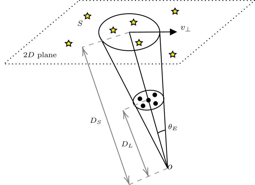
Figure 1: Demonstration of the lens-source geometry adopted in Section 3. The lenses and sources are at distances $D_{L}$ and $D_{S}$, respectively, from the observer $O$ along the line of sight. All the lenses and source stars are projected onto the two-dimensional plane of the sky. To compute the microlensing rate as the lens moves along this plane, we count the number of sources that lie within the area swept out by the Einstein ring (with diameter $2R_{E}$) at any point during the observing time interval.

3.2 Numerical calculations of self-lensing rates

We numerically compute the self-lensing rates in our cluster models similarly to Griest_1991; Zaris_2020. This method is more exact and accurate than the approximate analytical approach presented in the previous section but is limited to sources within the cluster (self-lensing). First we project the positions, $r$, and tangential and radial velocities, $v_{t}$ and $v_{r}$, respectively, of each object onto two dimensions, with angular coordinates assigned randomly on the unit sphere.

We imagine an Einstein ring attached to a lens moving across the corresponding sky-projected plane at a constant relative velocity, $v_{\perp}$, over an observing duration $T_{\rm obs}$ and check if the broad pass of the Einstein ring intersects with the position of a source (see Figure 1). The area swept out on the ‘sky’ by the lens will cover a narrow, nearly rectangular area across the plane perpendicular to the line of sight. We choose $T_{\rm obs}$ small enough that the lens only moves a small fraction of the cluster radius (enabling the projected trajectory to reasonably be described by a straight line) but large enough that the probability it will pass through a source is non-negligible. Finally, we compute the total microlensing rate by counting up the number of source stars inside the microlensing tube of radius $R_{E}=\theta_{E}D_{S}$ in the source plane and length $v_{\perp}T_{\rm obs}$ and then dividing by $T_{\rm obs}$.

4 Results

4.1 The CMC Cluster Catalog

In this section, we present our self-lensing rate estimates for the 10 CMC Cluster Catalog models. Table 2 lists for each model the total numbers of source stars $N_{\star}$ and various lens populations as well as the corresponding total event rates $\Gamma_{\rm tot}$ in units of events per year per $N_{\star}$. A quick glance confirms the natural expectation that the microlensing event rates are highest in clusters with the highest numbers of sources and lenses. As the numbers of both lens and source stars decrease, the microlensing event rates decrease by nearly the same factor. This trend is also evident in Figure LABEL:fig:mass_dist_catalog showing the relative contributions from lenses of different masses and radial positions in the cluster to the total self-lensing rates for three CMC Cluster Catalog models with different initial $N$. We see that the objects in the mass range $\simeq 0.1-0.7\,M_{\odot}$, which represent WDs and M dwarfs, dominate the microlensing rates. This is unsurprising since they dominate the cluster mass function at late times. Furthermore, as the initial $N$ increases, more NSs and BHs are retained and contribute to the microlensing rate. In Figure LABEL:fig:scatter_all, we show the mass and radial distributions of the different types of lenses that produce an observable event in the model n32-rv1-rg20-z0.01 with initial $N=3.2\times 10^{6}$ and virial radius $r_{v}=1\,$pc. As the lightest lenses we consider here ($\simeq 0.1\,M_{\odot}$), M dwarfs in this massive cluster are located mostly beyond the half-mass radius (4 pc), well into the cluster halo. Among various types of WDs, carbon-oxygen WDs, with average mass $0.75\,M_{\odot}$, produce the highest microlensing rate since they dominate by number. They are massive enough to segregate toward the cluster center, but only slightly so. The same is true for the NSs, with average mass $1.3\,M_{\odot}$, but the BHs reside much deeper in the cluster potential given their much higher average mass ($15\,M_{\odot}$).

Table 2: Self-lensing event rates of various lens populations in all model GCs

	Simulation	$N_{\star}$	$N_{\rm MD}$	$N_{\rm WD}$	$N_{\rm NS}$	$N_{\rm BH}$	$\Gamma_{\rm MD}$	$\Gamma_{\rm WD}$	$\Gamma_{\rm NS}$	$\Gamma_{\rm BH}$
							yr${}^{-1}$	yr${}^{-1}$	yr${}^{-1}$	yr${}^{-1}$
1	n8-rv0.5-rg8-z0.1	274944	232688	76753	273	1	0.004	0.01	8$\times 10^{-5}$	$<10^{-5}$
2	n16-rv0.5-rg8-z0.1	600279	537756	161703	740	64	0.04	0.05	6$\times 10^{-4}$	2$\times 10^{-4}$
3	n8-rv1-rg8-z0.1	300847	271497	80989	238	21	0.005	0.005	5$\times 10^{-5}$	2$\times 10^{-5}$
4	n16-rv1-rg8-z0.1	626541	578016	164008	610	207	0.03	0.03	4$\times 10^{-4}$	3$\times 10^{-4}$
5	n32-rv1-rg20-z0.01	1263364	1188229	343463	4901	962	0.1	0.1	0.002	0.003
6	n8-rv2-rg8-z0.1	314259	289919	81065	160	110	0.003	0.002	2$\times 10^{-5}$	3$\times 10^{-5}$
7	n16-rv2-rg8-z0.1	640980	598069	164674	449	534	0.02	0.01	2$\times 10^{-4}$	3$\times 10^{-4}$
8	n32-rv2-rg20-z0.01	1286873	1220092	345888	4160	1866	0.08	0.06	0.001	0.003
9	n8-rv4-rg8-z0.1	316884	293302	79556	74	297	0.001	0.001	$<10^{-5}$	2$\times 10^{-4}$
10	n16-rv4-rg8-z0.1	651299	610092	164273	335	979	0.008	0.005	1$\times 10^{-5}$	3$\times 10^{-4}$
11	47 Tuc	1209403	344100	447959	1298	159	0.03	0.2	0.002	4$\times 10^{-4}$
12	M22	291315	259255	76867	478	40	0.004	0.005	4$\times 10^{-5}$	2$\times 10^{-5}$

Note. — The total number of source stars $N_{\star}$, M dwarfs $N_{\mathrm{MD}}$, white dwarfs $N_{\mathrm{WD}}$, neutron stars $N_{\mathrm{NS}}$, and black holes $N_{\mathrm{BH}}$ at 12, 10.2, 10.9 Gyr for all CMC Catalog models, 47 Tuc and M22, respectively. The microlensing rate of each lens population is obtained numerically for a given total number of source stars $N_{\star}$ in all model GCs.