Conformal Hypergeometry and Integrability

Abstract.

Conformal field theories play a central role in modern theoretical physics with many applications to the understanding of phase transitions, gauge theories and even the quantum physics of gravity, through Maldacena’s celebrated holographic duality. The key analytic tool in the field is the so-called conformal partial wave expansion, i.e. a Fourier-like decomposition of physical quantities into a basis of partial waves for the conformal group SO$(1,d+1)$. This text provides an non-technical introduction to conformal field theory and the conformal bootstrap program with some focus on the mathematical aspects of conformal partial wave expansions. It emphasises profound relations with modern hypergeometry, group theory and integrable models of Gaudin and Calogero-Sutherland type.

1. Introduction

During the last century physicists gradually learned to appreciate the importance of conformal symmetry for our understanding of nature. By definition, conformal symmetry is made up of angle preserving transformations. The most commonly observed (conformal) symmetries are rotations and translations. These are present in all homogeneous and isotropic systems. Beyond that, dilations (scale transformations) are the most prominent examples of conformal transformations. Scale invariance is an important phenomenon in physics that refers to situations in which the features of a system do not change upon zooming in or out. The first known occurrence in nature is the critical point for the liquid-vapour transition in the phase diagram of water. Many more of these points have been discovered in the meantime. Some of them can be realized in spin systems such as the famous Ising model.

Particle physicists started to appreciate conformal field theories (CFTs) through the influential work of Wilson on the renormalization group [74]. By construction, scale invariance occurs at all fixed points of renormalization group transformations. This gives CFTs a very special status within the space of all theories, and makes them a good starting point to explore, in particular, non-perturbative phenomena in quantum field theory. More recently, CFTs became the main actors on another stage, Juan Maldacena’s celebrated AdS/CFT duality [47]. Its most general formulation proposes an equivalence between non-gravitational quantum systems in $d$ dimensions and gravitational systems in one dimension higher. In this context, a $d$-dimensional CFT is like a holographic screen for a gravitational theory in Anti-deSitter (AdS) space. As we make progress in dealing with CFTs, the AdS/CFT duality can be applied to provide novel views on the deep mysteries of a quantum theory of gravity, such as the phenomenon of Hawking radiation and black hole information.

The very brief history of scale/conformal invariance in physics that I presented in the first two paragraphs may serve one main purpose: it explains why a significant part of modern theoretical physics research is devoted to CFTs and why the interest ranges over so many different communities, from condensed matter theory and modern material science all the way to particle physics and quantum gravity.

Invariance under conformal transformations turns out to be a surprisingly powerful symmetry principle that strongly constrains physical observables such as the correlations between different measurements. These constraints may be exposed with the help of the most important analytical tool of CFT, the so-called conformal partial wave expansions. One should think of these as an extension of Fourier analysis, but for systems with conformal rather than mere translational symmetry. Just as plane waves in Fourier analysis are uniquely characterized by their behaviour under translations, conformal partial waves are determined by conformal symmetry alone, i.e. they belong to the realm of group and representation theory.

When conformal field theories were considered for the first time about 50 years ago, the relevant group theory was very far from being developed, which halted initial progress. This changed only after physicists started to focus on $d=2$ dimensions where conformal symmetry becomes infinite dimensional. For that case a very beautiful theory was developed with many deep relations to mathematics and integrable systems. But this is not our topic here. Instead, what I shall describe below is relevant for CFTs in dimension $d>2$. At the end of the last century, and in particular with the discovery of the AdS/CFT duality, the case for studying CFTs in $d>2$ had become so strong that physicists made another effort to develop at least some of its group theoretic foundations. The influential work of Dolan and Osborn [16, 17] on conformal partial waves for scalar 4-point functions and some subsequent work by other authors, see in particular [35, 45, 44, 57], eventually provided a basis for some new breakthrough developments in higher dimensional CFT, e.g. for the 3-dimensional critical Ising model.

At the time, physicists did not know that essentially all the required results on conformal partial waves were already contained in the seminal papers of Heckman and Opdam, see [31, 54, 30]. Somewhat surprisingly, before it was uncovered in [37], the profound relation went unnoticed between the study of integrable quantum mechanics of Calogero-Moser-Sutherland type on the one hand and conformal partial waves on the other. The main intent of this text is to help reduce the apparent and unfortunate divide between the physics communities that work on conformal field theories on the one hand and mathematicians with expertise in modern group theory, harmonic analysis, hypergeometry and integrability on the other. The study of CFTs continues to challenge profound advances of its group theoretic ingredients. So it is not too late for the relevant communities to join forces.

After these introductory remarks, let me describe the plan of this short note. The next section is meant as a smooth introduction to some basic notions of critical systems and CFT. In the example of the critical Ising model I will outline how statistical systems can become critical and possibly conformal. In addition, I shall introduce the notions of (scalar and spinning) fields, correlation functions, scaling weights, conformal partial waves etc. and I will sketch the main idea of the so-called conformal bootstrap program. Section 2 remains very descriptive, without precise definitions. Nevertheless, I hope that it can build a first intuition into the basic concepts of the area, in a spirit that is relatively close to the physicists’ approach. In section 3, I then rephrase the basic setup in a more mathematical language. There, the notions of fields, correlation functions and conformal partial waves are embedded into group theory and harmonic analysis. Once this is achieved, we can walk along well trodden paths into the world of hypergeometry and integrable systems. We will see the first examples of the relation between conformal partial waves and hypergeometry at the end of section 3. As I will argue there, conformal partial waves for scalar 4-point functions can be identified with the wave functions of hyperbolic Calogero-Moser-Sutherland models for the root system $BC_{2}$, i.e. these conformal partial waves are (close relatives of) $BC_{2}$ Heckman-Opdam hypergeometric functions. I conclude section 3 with a lightning overview of extensions which are more or less well understood, or at least have been actively researched already.

The final section is then devoted to a new important direction about which very little seems to be known for now: multipoint correlation functions. In a CFT, correlations of up to $N=3$ local measurements are essentially determined by conformal symmetry. Hence, the first non-trivial correlations that can be analysed with well studied conformal partial waves appears when $N=4$. The territory we shall begin to explore in the final section lies just one step beyond. For $N>4$, conformal partial waves were largely unexplored until very recently. Section 4 embeds the profound mathematical challenges in gaining control of these objects into the context of $N$-site Gaudin integrable models for the conformal group [6]. As I will discuss in detail, the study of the relevant conformal partial waves requires us to consider certain limits of the Gaudin integrable models which extend the so-called caterpillar or bending flow limits previously considered in [13, 14, 67]. In the final subsection I highlight an intriguing new appearance of the lemniscatic elliptic Calogero-Moser-Sutherland model of [20] in the context of $N$-point scalar conformal blocks or, equivalently, in limits of $N$-site Gaudin integrable models.

While sections 2 and 3 of this note survey developments from several decades and do not contain any new results, section 4 is based on some very recent research in collaboration with I. Buric, S. Lacroix, J.A. Mann and L. Quintavalle [5, 7].

Acknowledgments: I wish to thank my co-authors Ilija Buric, Misha Isachenkov, Sylvain Lacroix, Pedro Liendo, Yanick Linke, Jeremy Mann, Lorenzo Quintavalle, Evgeny Sobko for the inspiring collaboration on the material presented in this note. At the same time I am very grateful to the organizers of the workshop “Hypergeometry, Integrability and Lie Theory” at the Lorentz Center in Leiden for giving me the opportunity to present our work and to Jasper for providing the occasion. I have profited very much from many insightful questions, comments and discussions with participants during and after the meeting. This applies in particular to some of the new material included in the final subsection which has been stimulated by discussions with Pavel Etingof.

2. Conformal Field Theory and Partial Waves

2.1. The critical Ising model

As we have discussed in the introduction, conformal field theories are used to describe the critical behavior of many statistical systems. One of the most well known is the Ising model. Let us use this simple model to illustrate some of the key concepts. The Ising model can be defined on a $d$-dimensional hypercubic lattice with lattice sites given by $x_{n}=n^{\mu}\epsilon_{\mu}\in\mathbb{R}^{d}$. Here the summation over $\mu=1,\dots,d$ is understood and $\epsilon_{\mu}=\epsilon e_{\mu}$ coincide with the unit vectors $e_{\mu}$ of $\mathbb{R}^{d}$ up to a common scale factor $\epsilon$. We refer to $\epsilon$ as the lattice spacing. The coefficients $n^{\mu}$ are integers.

To each lattice site we now assign a spin $\sigma_{n}\in\{\pm 1\}$. Any such choice of spin assignments on all lattice sites is referred to as a spin configuration. The object $\sigma$ is (a discrete version) of what physicists call a field. In order to define our theory we must specify a measure on the on the space of configurations. For the Ising model, this measure is

(2.1) $$P_{\zeta}(\{\sigma\})=\mathcal{N}e^{\zeta\sum_{\langle nm\rangle}\sigma_{n}\sigma_{m}}\ .$$

Here the sum extends over nearest neighbors $\langle nm\rangle$, i.e. over all pairs of lattice sites that are a distance $|x_{n}-x_{m}|=\epsilon$ apart.

The nature of a typical configuration selected by the measure (2.1) depends very much on the value of the parameter $\zeta$. If we set $\zeta=0$, for example, neighboring spins do not interact, i.e. the value the measure assumes is the same on all spin configurations. Hence, if we measure the spin at site $n$, this won’t tell us anything about the value of the spin at another site $m$, in other words there is no correlation between the value $\sigma_{n}$ of the spin at site $n$ and the value of $\sigma_{m}$ at another sites $m\neq n$ of the lattice. In the opposite case with $\zeta=\infty$, configurations in which spins assume different values are infinitely suppressed, i.e. the measure only allows for the two constant configurations $\sigma_{n}=1$ or $\sigma_{n}=-1$ for all sites $n$. In this case, the correlations between spins are as strong as they can be. We only need to measure the spin $\sigma_{n}$ at one site $n$ to know its value at all the other sites $m\neq n$. Once we go away from this extreme case, spin flips are possible but still costly. In other words, while the measure still assumes its maximum value on the two constant configurations, it becomes less strongly peaked as we decrease $\zeta$. Consequently, spin configurations with large ‘islands’ of aligned spins will start to play a role. As we reduce the value of $\zeta$, smaller islands contribute. It turns out that, for some very special value $\zeta=\zeta_{c}$, islands of all sizes appear with equal probability. At this very special point, the system appears to be self-similar on scales that are large compared to the lattice spacing $\epsilon$ (and small compared to the overall size $L$ of the lattice if we consider a finite lattice). It is this ‘critical’ value $\zeta=\zeta_{c}$ of the parameter $\zeta$ that we want to focus on.

In order to probe the Ising model, physicists measure correlations between spins. The simplest interesting example is the correlation between two spins $\sigma_{n}$ and $\sigma_{m}$ at two different lattice sites $n,m$. The quantity is defined as

(2.2) $$\langle\sigma_{n}\sigma_{m}\rangle_{\zeta}=\sum_{\{\sigma\}}P_{\zeta}(\{\sigma\})\,\sigma_{n}\sigma_{m}\ .$$

To make this sum well defined, one can imagine that it is carried out on a finite lattice with $L^{d}$ lattice sites, even though criticality requires $L$ being sent to infinity at the end. As $\zeta$ approaches $\zeta_{c}$ the system becomes self-similar in the sense described above and hence this correlation function must take the form

(2.3) $$\langle\sigma_{n}\sigma_{m}\rangle_{\zeta_{c}}\sim\frac{1}{|x_{n}-x_{m}|^{2\Delta_{\sigma}}}\ .$$

Here, $|x_{n}-x_{m}|$ denotes the Euclidean distance between the lattice points $x_{n}$ and $x_{m}$ in $\mathbb{R}^{d}$. The $\sim$ means the function on the right hand side approximates the correlation function on intermediate scales or, equivalently, in the limit of an infinite lattice size $L$ and vanishing lattice spacing $\epsilon$. The parameter $\Delta_{\sigma}$ that describes how the correlation function falls off as we increase the distance between the two lattice sites is referred to as the scaling weight of $\sigma$. It is a very important observable of the critical system.

Determining the value of $\Delta_{\sigma}$ is one of the central challenges of CFT. In $d=2$ dimensions, it is possible to give an exact value. As was observed in [3], the scaling weight of the spin field in the critical 2-dimensional Ising model can be calculated using representation theory of the Virasoro algebra with central charge $c=1/2$. This approach famously gives

(2.4) $$\Delta^{\textrm{[2D]}}_{\sigma}=1/8\ .$$

For the 3-dimensional critical Ising model, the exact value of the scaling weight $\Delta_{\sigma}$ is not known, but there exist good numerical simulations (NSs) of the correlation (2.2) near $\zeta=\zeta_{c}$ that give the approximate result [29]

(2.5) $$\Delta^{\textrm{[3D],NS}}_{\sigma}\sim 0.51813(5)\ .$$

Let us point out right away that a more precise value of this exponent is known by now. However, this precision determination is based not on numerical simulation of the Ising model, but rather on the conformal bootstrap program that we shall outline below.

Before we go there, let us briefly mention that the scaling weight $\Delta_{\sigma}$ of the spin field $\sigma$ is not the only field in the Ising model. Obviously, it is possible to construct many similar quantities. To give just one additional example, let us introduce the object

(2.6) $$\varphi^{\mu}_{n}=\sigma(x_{n})\nabla^{\mu}\sigma(x_{n})=\sigma(x_{n})\sigma(x_{n}+\epsilon_{\mu})-1\ .$$

Note that the definition of $\varphi^{\mu}$ depends on the choice of a direction $\mu$ in the $d$-dimensional space. Physicists refer to $\varphi^{\mu}$ as a vector field as opposed to the spin field $\sigma$ which is scalar, i.e. does not single out any direction. One can go further and consider fields that are sensitive to the value of the Ising spin at more than two sites. The relevant sites may fall into a local cluster or be located along lines, surfaces, etc. One calls the associated objects local, line, surface operators, respectively. These operators can be inserted into correlation functions of the form (2.2), just as we did for the spin field $\sigma$. It turns out that the 2-point correlations of local operators also fall off with some characteristic exponent $\Delta_{\varphi}$ whose value depends on the field $\varphi$ that is inserted.

2.2. Conformal field theory

Critical systems are included in the wider class of homogeneous and isotropic systems which are invariant under translations $x^{\mu}\mapsto x^{\mu}+a^{\mu}$ and rotations $x^{\mu}\mapsto O^{\mu}_{\,\nu}x^{\nu}$ of points $x=(x^{\mu})\in\mathbb{R}^{d}$. As we have described above, the characteristic feature of critical system is self-similarity, i.e. at the critical point the symmetry is enhanced to include scale transformations $x^{\mu}\mapsto\lambda x^{\mu}$ with $\lambda\in\mathbb{R}^{+}$. It turns out, however, that the symmetry of many critical systems, including the critical Ising model, is further enhanced to the $d$-dimensional conformal group $SO(1,d+1)$. In addition to translations, rotations and scale transformations, the conformal group possesses $d$ generators of so-called special conformal transformations. This enhancement has dramatic consequences as we shall discuss now.

To begin exploring these consequences let us point out that in a conformal field theory, correlation functions of three fields are fixed by symmetry, up to some overall constant. This follows from the well known fact that conformal transformation can be used to map any set of three points in $\mathbb{R}^{d}$ to the values $x_{1}=0,x_{2}=\vec{e}_{1},x_{3}=\infty$. Hence, a 3-point function of scalar fields $\phi_{i}$ of scaling weight $\Delta_{i}$ must take the form

(2.7) $$\langle\phi_{1}(x_{1})\phi_{2}(x_{2})\phi_{3}(x_{3})\rangle=\frac{\gamma_{123}}{|x_{12}|^{\Delta_{12,3}}|x_{23}|^{\Delta_{23,1}}|x_{13}|^{\Delta_{13,2}}}=\gamma_{123}\includegraphics[width=56.9055pt,valign={c}]{scalarvert.png}$$

where $x_{ij}=x_{i}-x_{j}$ and $\Delta_{12,3}=\Delta_{1}+\Delta_{2}-\Delta_{3}$ etc. In more mathematical terms, the $x_{i}$-dependent function on the right hand side may be thought of as Clebsch-Gordon coefficients for the conformal group and the prefactors $\gamma_{123}$ provide a multiplication table for scalar fields of the theory. This is the interpretation we have tried to stress in the symbolic representation of the 3-point function on the right hand side.

What is so special about conformal field theories is indeed that their ‘multiplication table’ is really just a set of constants. To avoid confusion we need to stress that the ‘multiplication’ does not close on scalar fields, i.e. 3-point functions of two scalars and one vector field, for example, can be non-vanishing. But this does not alter the basic conclusion that conformal symmetry guarantees that there exists a ‘multiplication table’ of constants. It was already observed in the early days of CFT that the multiplication table of conformal field theories must obey stringent consistency conditions that are reminiscent of associativity constraints on multiplication tables in algebra. This observation is the main content of Polyakov’s conformal bootstrap program [61]. The concrete implementation of this program, however, is rather difficult and so far analytic solutions were only found for 2-dimensional conformal field theories. Nevertheless, the modern conformal bootstrap has led to profound new insights on conformal field theories in $d\geq 3$, see below.

2.3. Conformal partial waves and the bootstrap

The most basic associativity constraints arise from the study of 4-point correlation functions. These are no longer determined by conformal symmetry alone simply because one can form two independent conformally invariant cross ratios from four points in $\mathbb{R}^{d}$. We shall parametrize these through two variables $u_{1}$ and $u_{2}$. In order to analyse 4-point functions it is useful to expand them in terms of a ‘basis’ of conformal partial waves

(2.8) $$\langle\prod_{i=1}^{4}\phi_{i}(x_{i})\rangle\sum_{\Delta,l}\gamma_{12;\Delta,l}\gamma_{34;\Delta,l}G_{\Delta,l}(u_{1},u_{2})$$

Here the sum extends over all primary (= non-derivative) fields of scaling weight $\Delta$ and spin $l$, i.e. over fields that possess $l$ symmetric vector indices $\mu_{1},\dots,\mu_{l}$. Note that the coefficients $\gamma$ are part of the multiplication table, though they also include multiplication of scalar fields into fields that carry spin, unlike the coefficients we introduced in eq. (2.7). Generalizing the graphical notation we introduced in eq. (2.7) we can write such 3-point functions as

(2.9) $$\langle\phi_{1}(x_{1})\phi_{2}(x_{2})\Phi_{3}(x_{3})\rangle=\gamma_{12;\Delta,l}\includegraphics[width=65.44142pt,valign={c}]{SSSTTvert.png}\ .$$

The Clebsch-Gordan coefficients for two scalar and one spinning field are certainly known explicitly. But since we won’t need such detail, we shall content ourselves with the graphical notation. The conformal partial waves that appear in the expansion (2.8) of the scalar 4-point function can be considered as 4-point Clebsch-Gordan maps of the form

(2.10) $$G_{\Delta,l}=\includegraphics[width=71.13188pt,valign={c}]{scalar4point.png}\ .$$

The graphical notation in this equation emphases the construction of the partial wave by contraction of two (3-point) Clebsch-Gordan coefficients. One can actually translate this into a precise integral formula for $G$,

(2.11) $$G_{\Delta,l}\sim\int d^{d}x_{0}x_{10}^{l+a-\Delta}x_{20}^{l-a-\Delta}x_{30}^{l-b+\Delta-d}x_{40}^{l_{b}+\Delta-d}\left(|\mu||\tilde{\mu}|\right)^{l}Y^{d}_{l}\left(\frac{\mu\cdot\tilde{\mu}}{|\mu||\tilde{\mu}|}\right)$$

where

(2.12) $$\mu=\frac{x_{10}}{x_{10}^{2}}-\frac{x_{20}}{x_{20}^{2}}\quad,\quad\tilde{\mu}=\frac{x_{40}}{x_{40}^{2}}-\frac{x_{30}}{x_{30}^{2}},$$

the parameters $a,b$ are determined by the weights $\Delta_{i}$ as $2a=\Delta_{2}-\Delta_{1}$, $2b=\Delta_{3}-\Delta_{4}$ and $Y^{d}_{l}$ denotes zonal spherical functions. We have also used the notation $x^{t}=|x|^{t}$ whenever elements $x\in\mathbb{R}^{d}$ are raised to some power $t$. The integral over $x_{0}\in\mathbb{R}^{d}$ takes care of the sum over intermediate states when we construct a 4-point invariant from two 3-point invariants. Since the relevant representations of the conformal group are infinite dimensional (see next section), the summation is most easily expressed as an integral over some insertion point $x_{0}$ of the intermediate field of weight $\Delta$ and spin $l$.

Before we discuss which special functions the integrals (2.11) integrate to we want to sketch one important application of conformal partial wave expansions that should suffice to illustrate their importance. The attentive reader might have noticed already that the expansion (2.8) breaks the symmetry of the correlation functions with respect to the permutation of the four scalar fields. The expansion we have displayed pairs the fields $\phi_{1}$ and $\phi_{2}$ together. This arbitrary choice is referred to as the choice of a channel. To match common convention, we shall use the term operator product expansion (OPE) channel from now on, though it would be more appropriate to call it a conformal partial wave (CPW) channel here. In any case, for $N=4$ scalar fields there are two more channels, in addition to the one we have displayed, for which $\phi_{1}$ is paired with either $\phi_{3}$ or $\phi_{4}$. Note that the conformal partial waves $G$ do depend on the choice of the OPE channel. But after summing the partial waves with the coefficients $\gamma$, the symmetry between the four fields should be restored. This provides an important consistency condition on the coefficients $\gamma$ that is known as crossing symmetry condition. The conformal bootstrap [61] is designed to exploit these constraints in order to compute observables of the theory, such as the values of the scaling weights $\Delta$ or the coefficients $\gamma$. The program has had incredible success in $d=2$ dimensions after the seminal paper of Belavin, Polyakov and Zamolodchikov [3]. During the last decade, the conformal bootstrap has seen an impressive revival in higher dimensions with new numerical as well as analytical incarnations, see [64, 63, 60, 18, 19] as well as [25, 42, 1, 2, 40, 41] for early contributions and [59, 70, 58] for reviews, though geared to physicists. This has produced many stunning new insights including record precision computations of critical exponents in the critical Ising model [46] through the numerical conformal bootstrap (nCB),

(2.13) $$\Delta^{\textrm{[3D],nCB}}_{\sigma}\sim 0.5181489(10)\ .$$

Note that the bootstrap analysis succeeded to increase the precision to which we know the scaling weight $\Delta_{\sigma}$ of the spin field of the Ising model in $d=3$ dimensions by two orders of magnitude, as compared to all the clever numerical simulations that had been developed over a long time. This celebrated result has triggered a tremendous amount of new research that uses the bootstrap program to compute observables in (super)conformal field theories in higher dimensions.

The determination of $\Delta_{\sigma}$ for the $d=3$ critical Ising model required very good knowledge of the conformal partial waves which need to be evaluated in a power series expansion around one special point $u_{1}^{\ast},u_{2}^{*}$ in the space of cross ratios to very high orders. When conformal partial wave expansions were first introduced in [23, 24] the partial waves remained elusive objects. The necessary mathematical results that made efficient evaluation of the partial waves possible were pretty much out of reach back then. Physicists wondered for more than three decades what kind of special functions conformal partial are in dimension $d>2$. They were interested to understand how partial waves depend on the cross ratios $u_{i}$, the parameters $\Delta,l$ of the ‘intermediate field’ and on the weights $\Delta_{i}$ of the external fields. When higher dimensional conformal field theories became a central research topic at the end of the last century, Dolan and Osborn found a way to address these questions. Their idea was to characterize the partial waves as eigenfunctions of Casimir differential operators [16]. By analysing these operators they were able to uncover many interesting properties and in particular to express conformal partial waves in even dimensions through sums of products of Gauss’ hypergeometric functions [16, 17]. After a number of relevant extensions [35, 45, 44, 57], this line of research provided enough control over the conformal partial waves to implement a numerical version of Polyakov’s bootstrap program.

The central observation of [37] implied later that all the results physicists had obtained on conformal partial waves for scalar 4-point functions must be contained in the seminal series of papers by Heckman and Opdam [33, 32, 53, 55], see also [30, 56]. From the vantage point of [38] it became clear that the conformal partial waves (2.11) are sums of Harish-Chandra functions associated with the root system $BC_{2}$ and very close relatives of the corresponding Heckman-Opdam hypergeometric functions. At this point we will leave the more physics oriented approach of the first section to explain the relation between conformal partial waves and hypergeometry in a more mathematical language that should be easier to follow than the original work on the subject.

3. Conformal Partial Waves and Hypergeometry

3.1. Group theoretic reformulation

In order to understand the natural home of conformal partial waves in hypergeometry, we now want to start translating the physics ingredients we described above into a more mathematical language, mostly in the context of group theory. Recall that the symmetry group of a CFT is $G=SO(1,d+1)$ (or some covering thereof). The fields we worked with in the previous sections were inserted at points $x$ in the $d$-dimensional space. Since the action of conformal transformations is transitive, it is clear that we can think of space as a quotient of the conformal group by the stabilizer of a single point. The latter is the parabolic subgroup $P$ that is generated by dilations, rotations and special conformal transformations. Dilations form a subgroup $SO(1,1)\subset G$ while rotations are elements of $SO(d)\subset G$. These act on $\mathbb{R}^{d}$ in the usual way and hence they act on the $d$-dimensional abelian subgroup $N\subset G$ that is generated by special conformal transformations. Altogether, the stabilizer $P$ of a single point takes the form $P=K\ltimes N$ where $K=SO(1,1)\times SO(d)$. Note that $K$ is not compact. From now on we shall think of a point $x$ as an element $x\in G/P$ in the quotient space of the conformal group $G$ and the parabolic subgroup $P$.

The next ingredient we need to transfer to mathematics is the notion of a field. Configurations of a scalar field $\phi$ of weight $\Delta$ are elements in the space $\Gamma_{\Delta}$ of sections of a line bundle over the quotient space $G/P$. More precisely, we define

(3.1) $$\Gamma_{\Delta}=\Gamma_{\Delta}(G/P)=\{f:G\rightarrow\mathbb{C}\,|\,f(gp)=\chi_{\Delta}(p^{-1})f(g)\}\ .$$

The object $\chi_{\Delta}$ is a character of the parabolic subgroup $P\subset G$ that is trivial on the subgroups $N$ and $R=SO(d)$. On the generator $D$ of scale transformations, on the other hand, the character $\chi_{\Delta}$ assumes the value $\chi_{\Delta}(D)=\Delta$. Note that $D$ is an element of the conformal algebra $\mathfrak{g}=\mathfrak{so}(1,d+1)$ and we did not distinguish in notation between a character of the conformal group and its Lie algebra. Let us also stress that the linear spaces $\Gamma_{\Delta}$ of sections come equipped with the left regular action of the conformal group. For generic values of $\Delta$ the representation of $G$ on $\Gamma_{\Delta}$ is irreducible and infinite dimensional.

After this preparation we can now state that an $N$-point correlation function may be considered as a conformally invariant element in the tensor product of $N$ spaces $\Gamma_{1},\dots,\Gamma_{N}$,

(3.2) $$\langle\varphi_{1}(x_{1})\cdots\varphi_{N}(x_{N})\rangle\in\left(\Gamma_{1}\otimes\cdots\otimes\Gamma_{N}\right)^{G}$$

where the superscript $G$ is used to denote the subspace of $G$-invariant elements. To be more precise, the correlation function itself is not invariant, but there exists a map from the correlation function to the associated invariant. The latter is mediated by multiplication with a certain function $\Omega(x_{i};\Delta_{i})$ of the insertion points $x_{i}$. While $\Omega$ is not unique, there exists a canonical choice [8].

3.2. Conformal partial waves as spherical functions

For the moment let us focus on the case with $N=4$ scalar field insertions. The space of 4-point conformal invariants can be evaluated in two steps. First we want to evaluate the tensor product of the tensor factors $\Gamma_{1}=\Gamma_{\Delta_{1}}$ and $\Gamma_{2}=\Gamma_{\Delta_{2}}$. The result we are going to spell out in a moment involves the following linear space

(3.3) $$\Gamma_{\Delta}(G/K)\cong\{f:G\rightarrow\mathbb{C}\,|\,f(gk)=\chi_{\Delta}(k^{-1})f(g)\}\ .$$

The definition is similar to the construction in eq. (3.1), except that the right covariance condition only involves elements of the subgroup $K\subset P\subset G$ of the conformal group. In an abuse of notation we have denoted the character of this subgroup $K$ by the same symbol $\chi_{\Delta}$ as in the case of the parabolic subgroup $P$ above. Note that the two sets of characters are related by restriction since we assumed the character of $P$ to be trivial on the abelian subgroup $N\subset P$. With this notation we can now state [15]

(3.4) $$\Gamma_{i}(G/P)\otimes\Gamma_{j}(G/P)\cong\Gamma_{\Delta_{ij}}(G/K)\quad$$

where $\Delta_{ij}=\Delta_{i}-\Delta_{j}$. We can put this formula to use in the following analysis of conformal invariants in the 4-fold tensor product,

$$\left(\Gamma_{\Delta_{1}}\otimes\Gamma_{\Delta_{2}}\otimes\Gamma_{\Delta_{3}}\otimes\Gamma_{\Delta_{4}}\right)^{G} \cong \left(\Gamma_{\Delta_{12}}(G/K)\otimes\Gamma_{\Delta_{34}}(G/K)\right)^{G}\noindent$$

$$\cong \Gamma_{\Delta_{12},\Delta_{43}}(K\backslash G/K)\ .$$

The final result is expressed in terms of the spaces

(3.5) $$\Gamma_{\Delta,\Delta^{\prime}}(K\backslash G/K)=\{f:G\rightarrow\mathbb{C}\,|\,f(k_{l}gk_{r})=\chi_{\Delta_{21}}(k_{l})\chi_{\Delta_{34}}(k_{r}^{-1})f(g)\}\ .$$

These consist of sections of a line bundle over the double coset space $G/\!\!/K$. It is not difficult to see that the left action of $K$ in $G/K$ is transitive with stabilizer subgroup $B=SO(d-2)$. It follows that the double coset space has dimension

$$\textit{dim}\,(G/\!\!/K)=\textit{dim}(G)-2\textit{dim}(K)+\textit{dim}(B)=2\ .$$

The double quotient $G/\!\!/K$ coincides with the space of conformally invariant cross ratios that can be build from $N=4$ points in $\mathbb{R}^{d}$ for $d\geq 2$.

3.3. Hypergeometry of conformal partial waves

It is obvious that the Laplace operator on the conformal group $G$ descends to the space $\Gamma(K\backslash G/K)$. The associated radial Laplacian has been constructed and studied extensively in the mathematical literature [28, 34]. In particular, it is well known [51, 52] to be intimately related the trigonometric/hyperbolic Calogero-Moser-Sutherland Hamiltonian [11, 72, 49]

(3.6) $$H_{\textrm{CS}} = -\sum_{i=1}^{2}\frac{\partial^{2}}{\partial u_{i}^{2}}+\frac{k_{m}(k_{m}-1)}{2}\left[\sinh^{-2}\left(\frac{u_{1}+u_{2}}{2}\right)+\sinh^{-2}\left(\frac{u_{1}-u_{2}}{2}\right)\right]$$

$$\hskip 28.45274pt+\sum_{i=1}^{2}\left[k_{l}(k_{l}-1)\sinh^{-2}(u_{i})+\frac{k_{s}(k_{s}+2k_{l}-1)}{4}\sinh^{-2}\left(\frac{u_{i}}{2}\right)\right]$$

associated to the roots system $BC_{2}$ with multiplicity parameters given by

(3.7) $$k_{s}=\Delta_{43}\ ,\quad k_{m}=\frac{1}{2}(\Delta_{21}-\Delta_{43}+1)\ ,\quad k_{l}=\frac{1}{2}(d-2)$$

for the short, middle and long roots, respectively. These Hamiltonians have also been discussed in the talks of Margit Rössler and Eric Opdam at the meeting. The line of reasoning we have outlined here now allows to draw an important conclusion: In the case of scalar 4-point functions, the sought after conformal partial waves are eigenfunctions of a Calogero-Moser-Sutherland Hamiltonian and hence they are closely related with Heckman-Opdam hypergeometric functions for the $BC_{2}$ root system. To be quite precise, the boundary conditions one has to impose in the case of conformal partial waves differ from those imposed in the work of Heckman and Opdam. The correct conditions are described in [38]. It turns out that conformal partial waves are a linear combination of four of the eight Harish-Chandra functions in the problem.

In spite of this minor difference, the relation with Heckman-Opdam hypergeometry can be used to deduce many important properties in conformal partial waves, see [38]. The position of poles and their residues can be obtained easily from those of the corresponding Harish-Chandra functions, see e.g. [30, 56]. To obtain series expansions we realized the partial waves as the $q\mapsto 1^{-}$ limit of virtual Koornwinder polynomials [62] and employed the binomial expansions of Koornwinder polynomials from [50] to perform the degeneration with the help of [71, 43], see appendix A of [38] for details. Interesting shift equations for the various parameters of partial waves, finally, arise from the bispectral duality [65] between the trigonometric Calogero-Moser-Sutherland model with the rational Ruijsenaars-Schneider model for the same root system [66]. In this way, all properties of conformal partial waves physicists needed to prepare for applications in the modern conformal bootstrap can be recovered with relatively little effort from results mathematicians had obtained at the end of the last century.

The relation between conformal partial waves and Calogero-Moser-Sutherland models was first observed in [37] based on a direct analysis of the Casimir operators in the work of Dolan and Osborn. The direct group theoretical explanation I have outlined in the previous section has been described in [69, 68], with inspiration from earlier work in particular by Feher [21].

This group theoretic approach to conformal partial waves admits many relevant extensions. Among them is the extension to correlation functions of fields with spin, i.e. fields that transform non-trivially under the action of the rotation group $SO(d)\subset G$. In the general setup we described, this extension can be implemented by replacing the characters $\chi_{\Delta}$ of the parabolic subgroup $P$ or its subgroup $K=SO(1,1)\times SO(d)$ in eqs. (3.1) and (3.3), respectively, by some finite dimensional representations. The radial Laplacians on the associated vector bundles over the double coset $G/\!\!/K$ have been worked out very explicitly [69, 68] for a few representations of the rotation group $SO(d)$ in $d=3,4$. A general theory of the Hamiltonians and their eigenfunctions remains to be developed, even though for applications in physics sufficient control has been achieved, see [12, 39] and further references therein.

Another very important extension is required to study superconformal field theories, i.e. quantum field theories in which the conformal Lie algebra $\mathfrak{g}=\mathfrak{so}(1,d+1)$ gets extended to a superconformal one. This is particularly important since most known conformal quantum field theories are actually supersymmetric, especially in dimension $d>3$. For superconformal algebras of type I a general theory is obtained in [9, 10]. It reduces the theory of superconformal partial waves to that of ordinary conformal partial waves for fields with spin, see previous paragraph. The CFT literature contains few results in superconformal partial waves, except for very exceptional choices of field insertions, see e.g. [9] for references to the physics literature.

There is one more extension we want to briefly mention before we conclude this section. So far we have mostly discussed correlation functions of fields $\varphi(x)$ that are inserted at a point $x$ in the $d$-dimensional Euclidean space $x\in\mathbb{R}^{d}$ or its conformal compactification. But physics applications require to also consider operators that are localized along higher dimensional geometries such as lines, surfaces etc. One such example are the famous Wilson line operators in conformal gauge theories. Such non-local operators (fields) can be treated within the same framework, except that the stabilizer group $P$ of a point $x$ gets replaces by the stabilizer group $P_{p}=SO(1,p+1)\times SO(d-p)\ltimes\mathbb{R}^{d}$ of some $p$-dimensional submanifold. In this context, 2-point correlation functions of non-local fields can be treated pretty much in the same way as the 4-point function of local fields. The theory of conformal partial waves for 2-point correlation functions of non-local fields in CFT has been developed systematically in [36]. Not surprisingly, it can be reduced to the study of the Laplace operator on double quotients of the form $K_{p}\backslash G/K_{p^{\prime}}$ with $K_{p}=SO(1,p+1)\times SO(d-p)$. Therefore it is related to Heckman-Opdam hypergeometric functions for root systems $BC_{n}$ with the rank $n$ given by

(3.8) $$n=\textit{min}\left(p+2,p^{\prime}+2,d-p,d-p^{\prime}\right)\ .$$

Note that the rank is $n=2$ in case at least one of the non-local fields is inserted along a surface of dimension $p=0$ and $d\geq 2$. Higher ranks appear e.g. for correlation functions of two line operators (i.e. $p=p^{\prime}=1$) in $4$-dimensional conformal field theories etc. The theory of the associated conformal partial waves is relatively well developed, but this time only due to its relations with $BC_{n}$ Heckman-Opdam theory [36].

4. Integrability of Multipoint Conformal Partial Waves

Now that have described the link between conformal partial waves and hypergeometry at the example of scalar 4-point functions and have sketched a few extensions at the end of the previous section, I want to dedicate the final section to one challenging new direction that is only beginning develop. In the study of concrete conformal field theories physicists often compute correlation functions of more than $N=4$ fields. And even though the conformal bootstrap in its original formulation is focused on 4-point functions, one could very well imagine an alternative program that is based multipoint partial waves. Note that associativity of an algebra can be studied either within the set of all products that one can form from four elements of some linear basis or, alternatively, by studying associativity for higher products of a set of generating elements in the algebra. Some first attempt to carry the conformal bootstrap into this direction was recently made in [4], though in a somewhat restricted setting.

From these short comments we can conclude that it is of significant interest to develop a theory of multipoint conformal partial waves for $N>4$ insertion points. The following exposition of the subject in the context of integrability is based on several recent publications and work in progress [6, 5, 7]. There have also been other activities in physics to study multipoint partial waves, in particular directly through their integral representations. The most recent list of references to this research can be found in [7].

To set the stage, let us state the well-known fact that the number of independent conformal invariants one can build from $N$ points on $\mathbb{R}^{d}$ is given by

(4.1) $$n_{\textit{cr}}(N,d)=\left\{\begin{array}[]{ll}\frac{1}{2}N(N-3)&N\leq d+2\\[8.53581pt] Nd-\frac{1}{2}(d+2)(d+1)&N>d+2\end{array}\right.$$

Following the approach we have described above, a complete characterization of the associated conformal partial waves requires the same number of independent commuting differential operators. As in the case of the 4-point function, the set of differential operators depends on the choice of an OPE channel, see below for a precise definition.

4.1. Gaudin integrable models

The main idea for how to construct a complete set of commuting differential operators for each OPE channel of an N-point function exploits an interesting relation with Gaudin integrable systems. In order to make precise statements we need a bit of background on Gaudin models [26, 27]. Let us begin with a central object, the so-called Lax matrix,

(4.2) $$\mathcal{L}(w)=\sum_{i=1}^{N}\frac{\mathcal{T}^{(i)}_{\alpha}T^{\alpha}}{w-w_{i}}=\mathcal{L}_{\alpha}(w)T^{\alpha}\ .$$

Here, $w_{i}$ are a set of complex numbers, $T_{\alpha}$ denotes a basis of generators of the conformal Lie algebra in $d$ dimensions and $T^{\alpha}$ its dual basis with respect to an invariant bilinear form. The object $\mathcal{T}^{(i)}_{\alpha}$ denotes the set of right invariant vector fields on the space $\Gamma^{\Delta_{i}}_{G/P}$.

Given some conformally invariant symmetric tensor $\kappa_{p}$ of degree $p$ one can construct a family $\mathcal{H}_{p}(w)$ of commuting operators as [22, 73, 48]

(4.3) $$\mathcal{H}_{p}(w)=\kappa^{\alpha_{1}\cdots\alpha_{p}}_{p}\mathcal{L}_{\alpha_{1}}(w)\cdots\mathcal{L}_{\alpha_{p}}(w)+\dots\ ,$$

where the dots represent correction terms expressible as lower degree combinations of the Lax matrix components $\mathcal{L}_{\alpha}(w)$ and their derivatives with respect to $w$. For $p=2$ such correction terms are absent. The correction terms are necessary to ensure that the families commute,

(4.4) $$[\,\mathcal{H}_{p}(w)\,,\,\mathcal{H}_{q}(w^{\prime})\,]=0\ ,$$

for all $p,q$ and all $w,w^{\prime}\in\mathbb{C}$. It is a well-known fact that these families commute with the diagonal action of the conformal algebra, i.e.

(4.5) $$[\,\mathcal{T}_{\alpha}\,,\,\mathcal{H}_{p}(w)\,]=0\quad\textit{ where }\ \mathcal{T}_{\alpha}=\sum_{i=1}^{N}\mathcal{T}_{\alpha}^{(i)}\ .$$

Hence the commuting families $\mathcal{H}_{p}(w)$ of operators descend to differential operators on functions of the $n_{\textit{cr}}(N,d)$ conformally invariant cross ratios.

4.2. OPE limits of the Gaudin model

At this point, the commuting families $\mathcal{H}_{p}(w)$ still contain $N$ continuous parameters $w_{i},i=1,\dots,N$. Without loss of generality we can set three of these complex numbers to some specific values, e.g. $w_{1}=0,w_{N-1}=1,w_{N}=\infty$ so that we remain with $N-3$ complex parameters our Gaudin Hamiltonians depend on. The set of differential equations which characterize conformal partial waves, on the other hand, should only depend on the discrete choice of an OPE channel. As we shall see now, any OPE channel determines a certain limit of the parameters $w_{i}$. In other words, the parameters $w_{i}$ are entirely fixed by the channel.

In order to make a precise statement, we need a bit of preparation. Let us pick some OPE channel $\mathcal{C}$ along with an (arbitrary) external edge in the diagram. The latter serves as a reference point and we shall assign it the label $N$. As this edge is external, it is attached to a unique vertex which we will denote by $\rho_{\ast}$. Such a choice of reference vertex defines a so-called rooted tree representation of the channel, see Figure 1 for a concrete example with $N=8$. We draw the OPE diagram on a plane, with the vertex $\rho_{\ast}$ situated at the top and with each vertex having two downward edges attached. The representation on a plane forces us to make a choice of which edges are pointing towards the left and which edges are pointing towards the right: this choice is arbitrary, and gives rise to what is called a plane (or ordered) representation of the underlying rooted tree.

Figure 1. Plane rooted tree representation of an OPE diagram with 8 external fields.

Obviously, each vertex $\rho\in V$ from the set $V$ of $N-2$ vertices of the OPE diagram defines a partition $\underline{N}=I_{\rho,1}\mathbin{\mathchoice{\leavevmode\vtop{\halign{\hfil$\m@th\displaystyle#$\hfil\cr\cup\cr\cdot\crcr}}}{\leavevmode\vtop{\halign{\hfil$\m@th\textstyle#$\hfil\cr\cup\cr\cdot\crcr}}}{\leavevmode\vtop{\halign{\hfil$\m@th\scriptstyle#$\hfil\cr\cup\cr\cdot\crcr}}}{\leavevmode\vtop{\halign{\hfil$\m@th\scriptscriptstyle#$\hfil\cr\cup\cr\cdot\crcr}}}}I_{\rho,2}\mathbin{\mathchoice{\leavevmode\vtop{\halign{\hfil$\m@th\displaystyle#$\hfil\cr\cup\cr\cdot\crcr}}}{\leavevmode\vtop{\halign{\hfil$\m@th\textstyle#$\hfil\cr\cup\cr\cdot\crcr}}}{\leavevmode\vtop{\halign{\hfil$\m@th\scriptstyle#$\hfil\cr\cup\cr\cdot\crcr}}}{\leavevmode\vtop{\halign{\hfil$\m@th\scriptscriptstyle#$\hfil\cr\cup\cr\cdot\crcr}}}}I_{\rho,3}$, with the sets $I_{\rho,j}$ formed by the labels of the external fields attached to the three branches of the vertex. We shall fix the labelling of the three branches using the plane rooted tree representation of the channel: choose the branch $I_{\rho,1}$ to be the one pointing to the bottom left while the branch $I_{\rho,2}$ is pointing the bottom right. By construction, the last branch $I_{\rho,3}$ then always points to the top and contains the reference point $N$. Let us also note that the vertices $\rho\neq\rho^{*}$ are associated with a unique internal edge, namely the one that points upward. Thereby the plane rooted tree representation allows us to identify the set $E$ of internal edges with $E\equiv V\setminus\{\rho^{*}\}$.

So far, vertices were just enumerated by an element $\rho\in V$. Once we have drawn the diagram in a plane, we can assign a sequence $s^{\rho}=(s^{\rho}_{1},s^{\rho}_{2},\dots,s^{\rho}_{\delta_{\rho}})$ of elements $s^{\rho}_{a}\in\{1,2\}$ to each vertex $\rho$. This sequence $s^{\rho}$ encodes the path from $\rho_{\ast}$ to $\rho$. It tells us whether we have to move to the left (for $s_{a}^{\rho}=1$) or right (for $s_{a}^{\rho}=2$) every time we reach a new vertex until we arrive at $\rho$ after $\delta_{\rho}$ steps. We shall also refer to the length $\delta_{\rho}$ of the sequence as the depth of the vertex and to $s^{\rho}$ as the binary sequence of $\rho$. Note that the top vertex $\rho_{\ast}$ has depth $\delta_{\rho_{\ast}}=0$.

In order to construct the limit of the Gaudin model associated with the OPE channel $\mathcal{C}$, we need now construct a polynomial $g_{\rho}(\varpi)$ for each vertex $\rho$. If $s^{\rho}$ is the binary sequence associated with the vertex $\rho$, the polynomial $g_{\rho}$ is defined as

(4.6) $$g_{\rho}(\varpi)=\sum_{a=1}^{\delta_{\rho}}\varpi^{a-1}\delta_{s_{a}^{\rho},2}\ .$$

Obviously the top vertex $\rho_{\ast}$ is assigned to $g_{\rho_{\ast}}(\varpi)=0$. The vertices of depth $\delta_{\rho}=1$ are associated with $g_{\rho_{1}}(\varpi)=0$ or $g_{\rho_{2}}(\varpi)=1$, depending on whether they are reached from $\rho_{\ast}$ by going down to the left ($\rho_{1}$) or to the right ($\rho_{2}$) etc.

Similarly, we can assign polynomials $f_{i}(\varpi)$ to each external edge $1\leq i<N$ at the bottom of the plane rooted tree. Once again, we can encode the path from $\rho_{\ast}$ down to the edge $i$ by a binary sequence $s^{i}=(s^{i}_{1},s^{i}_{2},\dots,s_{\delta_{i}}^{i})$. The length $\delta_{i}$ of the sequence $s^{i}$ is also referred to as the depth of the edge $i$. Now we introduce

(4.7) $$f_{i}(\varpi)=\sum_{a=1}^{\delta_{i}}\varpi^{a-1}\delta_{s^{i}_{a},2}+\varpi^{\delta_{i}}\delta_{s^{i}_{\delta_{i}},1}\ .$$

and set

(4.8) $$f_{N}(\varpi)=\varpi^{-1}$$

for the external edge of the reference field at the top of the plane rooted tree. We have thus set up all the necessary notation that is needed to construct the relevant scaling limits of the $N$-site Gaudin model that remove the dependence on the continuous parameters $w_{i}$

The main idea in defining the channel dependent limit is to set $w_{i}=f_{i}(\varpi)$ and to send $\varpi$ to zero. When we perform this limit of the objects $\mathcal{H}^{(p)}(w;w_{i})$ of the $N$-site Gaudin model we must adjust the spectral parameter $w$ and multiply with some appropriate powers of $\varpi$ in order to obtain sufficiently many independent commuting operator. More precisely, for given a vertex $\rho$ we introduce

(4.9) $$\mathcal{H}_{\rho}^{(p)}(w)=\lim_{\varpi\to 0}\varpi^{pn_{\rho}}\mathcal{H}^{(p)}\bigl{(}\varpi^{n_{\rho}}w+g_{\rho}(\varpi),w_{i}=f_{i}(\varpi)\bigr{)}\ .$$

It can be shown that the set of these objects with $\rho\in E$ indeed contain $n_{\textit{cr}}(N,d)$ independent operators on the space of conformal invariants. These include operators of the form

(4.10) $$\mathcal{C}^{(p)}_{\rho}=\lim_{w\to\infty}w^{p}\mathcal{H}_{\rho}^{(p)}(w)\quad\mathit{for}\quad\rho\neq\rho^{*}\ .$$

These measure the weight and spin of the field which is exchanged along the internal edge $\rho\in E$ above the vertex $\rho\neq\rho^{*}$. We refer to the operators $\mathcal{C}^{(p)}_{\rho}$ as Casimir operators of the edge $\rho$. For a given edge $\rho\neq\rho^{*}$ there can be relations between operators with different values of $p$. Taking these into account, the internal edge $\rho\neq\rho^{*}$ provides us with

(4.11) $$n_{\textit{Cas}}(\rho,d):=\textrm{min}\left(|I_{\rho,3}|,N-|I_{\rho,3}|,\textrm{rank}_{d}\right)=:\mathfrak{d}_{\rho}$$

independent operators. Here $|I|$ denotes the order of the subset $I\subset\underline{N}$ and $\mathrm{rank}_{d}$ is the rank of the $d$-dimensional conformal algebra. It is easy to see that for $N>4$, the integers $n_{\textit{Cas}}$ do not add up to $n_{\textit{cr}}$. This means that the Casimir operators do not suffice to characterize multipoint conformal partial waves. The missing operators can all be constructed from the objects (4.9). It turns out that given a vertex $\rho$ and an index $p$ one can prepare

(4.12) $$n_{\textit{vert}}^{(p)}(\rho,d)=\textit{max}\left[\left((p-2)-\sum_{e\in\overline{E}_{\rho}}^{3}\Theta_{0}(p-2\mathfrak{d}_{e})(p-2\mathfrak{d}_{e}-1)\right),0\right]\,,$$

additional independent vertex differential operators. Here $\Theta_{0}$ is the Heaviside step function with $\Theta_{0}(0)=0$ and $\overline{E}_{\rho}$ consists of all external and internal edges that have one endpoint at the vertex $\rho$. For internal edges $e=\rho^{\prime}$, the quantity $\mathfrak{d}_{e}$ was introduced as a shorthand in eq. (4.11) and for external edges we set $\mathfrak{d}_{e}=1$. The formula applies for all $p$ as long as $d$ is odd. It requires some adjustment in even $d$, see [7] for details and a derivation.

Given this counting of independent commuting differential operators it is now possible to check that

(4.13) $$n_{\textit{cr}}(N,d)=\sum_{\rho\neq\rho^{*}}n_{\textit{Cas}}(\rho,d)+\sum_{\rho}\sum_{p}n_{\textit{vert}}^{(p)}(\rho,d)\ ,$$

i.e. that the set of independent differential operators suffices to completely characterize the multipoint conformal partial waves.

The OPE limits we described here are generalizations of the so-called caterpillar or bending flow limits that have been considered in the mathematical literature, see e.g. [13, 14, 67]. The caterpillar limit corresponds to the special case of an OPE limit for which the OPE diagram has the shape of a comb, see Figure 2. Following our conventions in [6], we enumerate the vertices $\rho=[r]$ by an integer $r=1,\dots,N-2$ that is related to its depth $\delta_{\rho}=\delta_{[r]}$ as $\delta_{[r]}=N-2-r$.

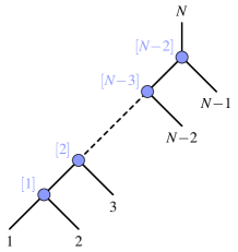
Figure 2. Choice of plane rooted tree representation of the comb channel OPE diagram with $N$ points.

One can compute the limit of the Gaudin model associated with this tree using the construction outlined in the previous subsection. For the polynomials $f_{i}$ that determine the parameters $w_{i}$ of the Gaudin model, one finds from eq. (4.7) that

(4.14) $$w_{i}=f_{i}(\varpi)=\varpi^{N-1-i},\qquad\forall\,i\in\{1,\cdots,N\}\ .$$

while all the vertex polynomials vanish, i.e. $g_{[r]}=0$ for $r=1,\dots,N-2$. Our general prescription (4.9) thus becomes

(4.15) $$\mathcal{H}_{[r]}^{(p)}(w)=\lim_{\varpi\to 0}\varpi^{p(N-2-r)}\mathcal{H}^{(p)}\bigl{(}\varpi^{N-2-r}w;w_{i}=\varpi^{N-1-i}\bigr{)}\ .$$

In order to illustrate our results and also prepare for the discussion in the next subsection we want to take a closer look at the case of $N=6$ points for $d>4$. According to equation (4.11), the three internal edges $[r],r=1,2,3,$ in the comb channel diagram contribute

(4.16) $$n_{\textit{Cas}}([1],d)=2=n_{\textit{Cas}}([3],d)\quad,\quad n_{\textit{Cas}}([2],d)=3$$

and hence a total number of $7$ Casimir differential operators. Our result (4.12), on the other hand shows that the four vertices $[r],r=1,\dots,4,$ contribute

(4.17) $$n_{\textit{vert}}^{(p)}([1],d)=0=n_{\textit{vert}}^{(p)}([4],d)\quad,\quad n_{\textit{vert}}^{(p)}([2],d)=1=n_{\textit{vert}}^{(p)}([3],d)$$

and hence a total of two vertex differential operators which are both of order four. When combined, the number of differential operators matches the number of $n_{\textit{cr}}=9$ cross ratios.

4.3. Relation with lemniscatic elliptic CMS model

The two inner vertices of the $N=6$ point partial wave are among the simplest vertices that carry degrees of freedom, i.e. for which $n_{\textit{vert}}\neq 0$. As one can infer from our general formula (4.12), it is in fact the unique vertex in $d>4$ that gives rise to a single parameter. Let us focus on the vertex $\rho=[2]$ of the $N=6$ point function, see our discussion at the end of the previous subsection, which connects the internal edges $[1]$ and $[2]$ with the external line $i=3$. According to our list (4.16), the edge $[2]$ admits two independent Casimir operators whose eigenvalues we parametrize through $\Delta_{1}$ and $l_{1}$. The internal edge $[3]$, on the other side, admits three independent Casimir operators. Their eigenvalues can be parametrized by three parameters $\Delta_{2},l_{2},\ell_{2}$. The external scalar edge comes with one parameter, namely the scaling weight $\Delta_{3}$ of the external scalar field. Let us note that for $d=4$, the vertex which we consider here is the special case of a single variable vertex with one additional parameter $\ell_{1}\neq 0$. On the other hand, if we specialize the non-trivial vertex of the $N=6$ point function to $\ell_{2}=0$ it can be considered down to $d=3$.

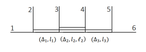
Figure 3. The two nontrivial vertices in the 6-point function are characterized by six quantum numbers each.

Our goal now is to identify the fourth order vertex differential operator for the single variable vertices. The easiest way to describe the findings of [7] involves a new algebra that is generated by operators $A,A^{\dagger}$ and $N$ which obey the following relations

(4.18) $$[N,A^{\dagger}]=A^{\dagger}\quad \quad[N,A]=-A\,,$$ ,

(4.19) $$AA^{\dagger}=R_{\alpha}(N+1)\quad \quad A^{\dagger}A=R_{\alpha}(N)$$ ,

where

$$R_{\alpha}(N)=\frac{N(N+2\alpha-1)}{(N+\alpha-1)(N+\alpha)}(N+\nu_{1}+2\alpha)(N-\nu_{1}-1)(N+\nu_{2}+2\alpha)(N-\nu_{2}-1)\,.$$

The algebra depends parametrically on the three spin parameters as $\alpha=\ell_{2}+(d-3)/2$ and $\nu_{k}=l_{k}-\ell_{2}$, but is independent of the conformal weights $\Delta_{i}$. The family of algebras comes equipped with an involutive anti-automorphism $\ast$ defined by $N^{\ast}=N$ and $A^{\ast}=A^{\dagger}$, provided that the parameters obey

(4.20) $$\bar{\alpha}=\alpha\,,\qquad\bar{\nu}_{1}=-(2\alpha+1+\nu_{1})\,,\qquad\bar{\nu}_{2}=-(2\alpha+1+\nu_{2})\,.$$

The vertex operator $H$ can now be written as a rational combination of the three generators as,

(4.21) $$H^{(d;\Delta_{i};l_{i};\ell_{i})}= B^{\dagger}B-\Gamma(N+\alpha)^{2}+\frac{\alpha(\alpha-1)\,K}{(N+\alpha)^{2}-1}+E^{(d;\Delta_{i};l_{k};\ell_{2})}.$$

Here, we defined the operators

(4.22) $$B^{\dagger}:= \frac{A-A^{\dagger}}{2\mathrm{i}}-\mathrm{i}(2\gamma_{1}\gamma_{2}+\mathrm{i}\gamma_{3})(N+\alpha)\,,$$

(4.23) $$B:= \frac{A-A^{\dagger}}{2\mathrm{i}}+\mathrm{i}(2\gamma_{1}\gamma_{2}-\mathrm{i}\gamma_{3})(N+\alpha)\,,$$

and the two parameters

(4.24) $$\Gamma:= \frac{1}{4}(1+4\gamma_{1}^{2})(1+4\gamma_{2}^{2})\,,$$

(4.25) $$K:= (\nu_{1}+\alpha)(\nu_{2}+\alpha)(\nu_{1}+\alpha+1)(\nu_{2}+\alpha+1)\,.$$

An expression for the constant term $E$ in our formula for the vertex operator (4.21) can be found in subsection 5.2 of [5]. The three parameters $\gamma_{i}$ that appear in the last few formulas are related to the conformal weights $\Delta_{i}$ of the three fields at the vertex as

$$\Delta_{i}=\frac{d}{2}+\mathrm{i}\gamma_{i}\ .$$

The operator $H$ is self-adjoint provided that the parameters $\gamma_{i}$ are real.

As one can easily check, the algebra generated by $A,A^{\dagger}$ and $N$ admits a representation in a basis $C_{n}^{(\alpha)}$ of the form

(4.26) $$NC_{n}^{(\alpha)} :=nC_{n}^{(\alpha)},$$

(4.27) $$AC_{n}^{(\alpha)} :=(n+\nu_{1}+2\alpha)(n+\nu_{2}+2\alpha)\frac{n+2\alpha-1}{n+\alpha}C_{n-1}^{(\alpha)}\,,$$

(4.28) $$A^{\dagger}C_{n}^{(\alpha)} :=(n-\nu_{1})(n-\nu_{2})\frac{n+1}{n+\alpha}C_{n+1}^{(\alpha)},$$

where eq. (4.27) applies to all integers $n>0$, and $AC_{0}^{(\alpha)}=0$ when $n=0$, i.e. the state $C_{0}^{(\alpha)}$ is annihilated by the lowering operator $A$. Similarly, the action of the raising operator $A^{\dagger}$ vanishes if $n=\nu_{1}$ or $n=\nu_{2}$. Consequently, one can restrict the action of $A,A^{\dagger}$ and $N$ to the finite dimensional subspace that is spanned by $C_{n}$ for $n=0,\dots,\mathrm{min}(\nu_{1},\nu_{2})$. When the basis is realized as Gegenbauer polynomials $C^{(\alpha)}(s)=C^{(\alpha)}(1-2\mathcal{X})$, the operators $A,A^{\dagger}$ describe the action of second order differential operators in the variable $\mathcal{X}$. We then showed that the resulting fourth order differential operator $H=H_{\mathcal{X}}$ can be mapped to the Hamiltonian $L$ of a crystallographic elliptic Calogero-Moser-Sutherland model that was discovered originally by Etingof, Felder, Ma and Veselov [20]. The latter acts on functions in a variable $z$ on the lemniscatic elliptic curve. We found the variables $\mathcal{X}$ to be related to $z$ as

(4.29) $$\mathcal{X}=\frac{\wp(1/2)^{2}}{\wp(1/2)^{2}-\wp(z)^{2}}\ ,$$

where $\wp$ is the Weierstrass elliptic function with lemniscatic periodicity conditions $\wp(z)=\wp(z+1)=\wp(z+i)$. Given this change of variables, our vertex Hamiltonian $H=H_{\mathcal{X}}$ and the elliptic CMS Hamiltonian $L=L_{z}$ of [20] are related as

(4.30) $$\Theta^{-1}H_{\mathcal{X}}\Theta\sim L_{z}$$

where

(4.31) $$\Theta\sim\,\mathcal{X}^{(l_{1}+l_{2}-2\ell_{2}+\Delta_{3}+(1-d)/2)/4}(1-\mathcal{X})^{(l_{1}+l_{2}-2\ell_{2}-\Delta_{3}+(1+d)/2)/4}\ .$$

The lemniscatic Calogero-Moser-Sutherland Hamiltonian $L$ involves seven parameters (multiplicities) whose values are determined by the three conformal weights $\Delta_{i}$, the spin parameters $l_{1},l_{2},\ell_{2}$ and the dimension $d$. Precise formulas can be found in [7]. A similar relation for a 3-point vertex with one scalar and two generic spinning legs of the $d=4$ dimensional conformal group also holds. In that case, the dimension $d$ is fixed and the seven multiplicities of the lemniscatic model $L$ are obtained from the three conformal weights and four spin variables $l_{1},\ell_{1},l_{2},\ell_{2}$, see [7] for precise formulas.

5. Concluding comments

This brings us to the end of this short note on higher dimensional CFT and its profound relation to multivariate hypergeometry. In the past, the interaction between these two fields has not lived up to its true potential. I hope that this text can make a modest contribution to developing a culture of mutual interest and understanding. It would clearly be very beneficial to join forces on overcoming some of the challenges that arise within CFT.

In my outline of concrete open problems I have focused on the study of multipoint partial waves, mostly because it is particularly timely and has seen some recent advances that are partly due to the very fruitful interactions I had during and after the workshop. Let me stress, however, that there are many other interesting problems that could profit from fresh mathematical input. One of these concerns the study of hypergeometric functions associated with (conformal) supergroups. I have only scratched this topic very briefly at the end of section 3. Given that most of the CFTs we know about are supersymmetric, progress in the theory of superconformal partial waves is guaranteed to have many applications. While physicists have made some advances over the last years, very much remains to be done.

References

- [1] Luis F. Alday, Agnese Bissi, and Tomasz Lukowski, Large spin systematics in CFT, JHEP 11 (2015), 101.
- [2] Luis F. Alday and Alexander Zhiboedov, Conformal Bootstrap With Slightly Broken Higher Spin Symmetry, (2015).
- [3] A.A. Belavin, Alexander M. Polyakov, and A.B. Zamolodchikov, Infinite Conformal Symmetry in Two-Dimensional Quantum Field Theory, Nucl.Phys. B241 (1984), 333–380.
- [4] Carlos Bercini, Vasco Gonçalves, and Pedro Vieira, Light-Cone Bootstrap of Higher Point Functions and Wilson Loop Duality, Phys. Rev. Lett. 126 (2021), no. 12, 121603.
- [5] Ilija Buric, Sylvain Lacroix, Jeremy Mann, Lorenzo Quintavalle, and Volker Schomerus, Gaudin Models and Multipoint Conformal Blocks: General Theory, JHEP 10 (2021), 139.
- [6] Ilija Buric, Sylvain Lacroix, Jeremy A. Mann, Lorenzo Quintavalle, and Volker Schomerus, From Gaudin Integrable Models to -dimensional Multipoint Conformal Blocks, Phys. Rev. Lett. 126 (2021), no. 2, 021602.
- [7] by same author, Gaudin Models and Multipoint Conformal Blocks II: Comb channel vertices in 3D and 4D, (2021).
- [8] Ilija Burić, Volker Schomerus, and Mikhail Isachenkov, Conformal Group Theory of Tensor Structures, JHEP 10 (2020), 004.
- [9] Ilija Buric, Volker Schomerus, and Evgeny Sobko, Superconformal Blocks: General Theory, JHEP 01 (2020), 159.
- [10] Ilija Burić, Volker Schomerus, and Evgeny Sobko, The superconformal -ing equation, JHEP 10 (2020), 147.
- [11] F. Calogero, Solution of the one-dimensional N body problems with quadratic and/or inversely quadratic pair potentials, J. Math. Phys. 12 (1971), 419–436.
- [12] Alejandro Castedo Echeverri, Emtinan Elkhidir, Denis Karateev, and Marco Serone, Seed Conformal Blocks in 4D CFT, JHEP 02 (2016), 183.
- [13] A. Chervov, G. Falqui, and L. Rybnikov, Limits of Gaudin algebras, quantization of bending flows, Jucys-Murphy elements and Gelfand-Tsetlin bases, Lett. Math. Phys. 91 (2010), 129–150.
- [14] Alexander Chervov, Gregorio Falqui, and Leonid Rybnikov, Limits of Gaudin Systems: Classical and Quantum Cases, SIGMA 5 (2009), 029.
- [15] V. K. Dobrev, G. Mack, V. B. Petkova, S. G. Petrova, and I. T. Todorov, Harmonic Analysis on the n-Dimensional Lorentz Group and Its Application to Conformal Quantum Field Theory, Lect. Notes Phys. 63 (1977), 1–280.
- [16] F.A. Dolan and H. Osborn, Conformal partial waves and the operator product expansion, Nucl.Phys. B678 (2004), 491–507.
- [17] by same author, Conformal Partial Waves: Further Mathematical Results, (2011).
- [18] Sheer El-Showk, Miguel F. Paulos, David Poland, Slava Rychkov, David Simmons-Duffin, et al., Solving the 3D Ising Model with the Conformal Bootstrap, Phys.Rev. D86 (2012), 025022.
- [19] by same author, Solving the 3d Ising Model with the Conformal Bootstrap II. c-Minimization and Precise Critical Exponents, J.Stat.Phys. xx (2014), xx.
- [20] Pavel Etingof, Giovanni Felder, Xiaoguang Ma, and Alexander Veselov, On elliptic Calogero-Moser systems for complex crystallographic reflection groups, Journal of Algebra 329 (2011), no. 1, 107–129, See also erratum 2.14 in http://www-math.mit.edu/~etingof/errorsinpapers.pdf.
- [21] L. Feher and B. G. Pusztai, Derivations of the trigonometric BC(n) Sutherland model by quantum Hamiltonian reduction, Rev. Math. Phys. 22 (2010), 699–732.
- [22] Boris Feigin, Edward Frenkel, and Nikolai Reshetikhin, Gaudin model, Bethe ansatz and correlation functions at the critical level, Commun. Math. Phys. 166 (1994), 27–62.
- [23] S. Ferrara, A. F. Grillo, G. Parisi, and R. Gatto, The shadow operator formalism for conformal algebra. Vacuum expectation values and operator products, Lett. Nuovo Cim. 4S2 (1972), 115–120.
- [24] S. Ferrara, A. F. Grillo, G. Parisi, and Raoul Gatto, Covariant expansion of the conformal four-point function, Nucl. Phys. B49 (1972), 77–98, [Erratum: Nucl. Phys.B53,643(1973)].
- [25] A. Liam Fitzpatrick, Jared Kaplan, David Poland, and David Simmons-Duffin, The Analytic Bootstrap and AdS Superhorizon Locality, JHEP 12 (2013), 004.
- [26] M. Gaudin, Diagonalisation d’une classe d’hamiltoniens de spin, Journal de Physique 37 (10) (1976), 1087–1098.
- [27] M. Gaudin, La fonction d’onde de Bethe, Masson, 1983.
- [28] Harish-Chandra, Collected papers, Springer, 1984.
- [29] Martin Hasenbusch, Finite size scaling study of lattice models in the three-dimensional Ising universality class, Phys. Rev. B 82 (2010), 174433.
- [30] G. Heckman and H. Schlichtkrull, Harmonic analysis and special functions on symmetric spaces, Academic Press, 1994.
- [31] G. J. Heckman, Root systems and hypergeometric functions. I-II, Compositio Mathematica 64 (1987), no. 3, 329–373 and 353–373.
- [32] by same author, Root systems and hypergeometric functions. ii, Compositio Mathematica 64 (1987), no. 3, 353–373.
- [33] G. J. Heckman and E. M. Opdam, Root systems and hypergeometric functions. i, Compositio Mathematica 64 (1987), no. 3, 329–373.
- [34] S. Helgason, Differential geometry, lie groups, and symmetric spaces, ISSN, Elsevier Science, 1979.
- [35] Matthijs Hogervorst and Slava Rychkov, Radial Coordinates for Conformal Blocks, Phys. Rev. D87 (2013), 106004.
- [36] Mikhail Isachenkov, Pedro Liendo, Yannick Linke, and Volker Schomerus, Calogero-Sutherland Approach to Defect Blocks, JHEP 10 (2018), 204.
- [37] Mikhail Isachenkov and Volker Schomerus, Superintegrability of -dimensional Conformal Blocks, Phys. Rev. Lett. 117 (2016), no. 7, 071602.
- [38] by same author, Integrability of conformal blocks. Part I. Calogero-Sutherland scattering theory, JHEP 07 (2018), 180.
- [39] Denis Karateev, Petr Kravchuk, and David Simmons-Duffin, Weight Shifting Operators and Conformal Blocks, JHEP 02 (2018), 081.
- [40] Apratim Kaviraj, Kallol Sen, and Aninda Sinha, Analytic bootstrap at large spin, JHEP 11 (2015), 083.
- [41] by same author, Universal anomalous dimensions at large spin and large twist, JHEP 07 (2015), 026.
- [42] Zohar Komargodski and Alexander Zhiboedov, Convexity and Liberation at Large Spin, JHEP 1311 (2013), 140.
- [43] T. H. Koornwinder, Okounkov’s BC-type interpolation Macdonald polynomials and their q=1 limit, ArXiv e-prints (2014).
- [44] Filip Kos, David Poland, and David Simmons-Duffin, Bootstrapping Mixed Correlators in the 3D Ising Model, JHEP 11 (2014), 109.
- [45] by same author, Bootstrapping the vector models, JHEP 06 (2014), 091.
- [46] Filip Kos, David Poland, David Simmons-Duffin, and Alessandro Vichi, Precision Islands in the Ising and Models, (2016).
- [47] Juan Martin Maldacena, The Large N limit of superconformal field theories and supergravity, Int. J. Theor. Phys. 38 (1999), 1113–1133.
- [48] A. I. Molev, Feigin-Frenkel center in types B, C and D, Inventiones Mathematicae 191 (2013), no. 1, 1–34.
- [49] J. Moser, Three integrable Hamiltonian systems connected with isospectral deformations, Adv. Math. 16 (1975), 197– 220.
- [50] A. Okounkov, BC-type interpolation Macdonald polynomials and binomial formula for Koornwinder polynomials, Transformation Groups 3 (1998), no. 2, 181–207.
- [51] M. A. Olshanetsky and A. M. Perelomov, Classical integrable finite dimensional systems related to Lie algebras, Phys. Rept. 71 (1981), 313.
- [52] by same author, Quantum Integrable Systems Related to Lie Algebras, Phys. Rept. 94 (1983), 313–404.
- [53] E. M. Opdam, Root systems and hypergeometric functions iii, Compositio Mathematica 67 (1988), no. 1, 21–49 (eng).
- [54] by same author, Root systems and hypergeometric functions III-IV, Compositio Mathematica 67 (1988), no. 1-2, 21–49 and 191–209.
- [55] by same author, Root systems and hypergeometric functions iv, Compositio Mathematica 67 (1988), no. 2, 191–209 (eng).
- [56] Eric M. Opdam, Part i: Lectures on dunkl operators, MSJ Memoirs, vol. Volume 8, pp. 2–62, The Mathematical Society of Japan, Tokyo, Japan, 2000.
- [57] João Penedones, Emilio Trevisani, and Masahito Yamazaki, Recursion Relations for Conformal Blocks, JHEP 09 (2016), 070.
- [58] David Poland, Slava Rychkov, and Alessandro Vichi, The Conformal Bootstrap: Theory, Numerical Techniques, and Applications, Rev. Mod. Phys. 91 (2019), 015002.
- [59] David Poland and David Simmons-Duffin, The conformal bootstrap, Nature Phys. 12 (2016), no. 6, 535–539.
- [60] David Poland, David Simmons-Duffin, and Alessandro Vichi, Carving Out the Space of 4D CFTs, JHEP 05 (2012), 110.
- [61] A.M. Polyakov, Nonhamiltonian approach to conformal quantum field theory, Zh. Eksp. Teor. Fiz. 66 (1974), 23–42.
- [62] Eric Rains, -symmetric polynomials, Transformation Groups 10 (2005), no. 1, 63–132.
- [63] Riccardo Rattazzi, Slava Rychkov, and Alessandro Vichi, Bounds in 4D Conformal Field Theories with Global Symmetry, J. Phys. A44 (2011), 035402.
- [64] Riccardo Rattazzi, Vyacheslav S. Rychkov, Erik Tonni, and Alessandro Vichi, Bounding scalar operator dimensions in 4D CFT, JHEP 0812 (2008), 031.
- [65] S. N. M. Ruijsenaars, Action Angle Maps and Scattering Theory for Some Finite Dimensional Integrable Systems. 1. The Pure Soliton Case, Commun. Math. Phys. 115 (1988), 127–165.
- [66] S. N. M. Ruijsenaars and H. Schneider, A New Class of Integrable Systems and Its Relation to Solitons, Annals Phys. 170 (1986), 370–405.
- [67] Leonid Rybnikov, Cactus group and monodromy of bethe vectors, (2016).
- [68] Volker Schomerus and Evgeny Sobko, From Spinning Conformal Blocks to Matrix Calogero-Sutherland Models, JHEP 04 (2018), 052.
- [69] Volker Schomerus, Evgeny Sobko, and Mikhail Isachenkov, Harmony of Spinning Conformal Blocks, JHEP 03 (2017), 085.
- [70] David Simmons-Duffin, The Conformal Bootstrap, Theoretical Advanced Study Institute in Elementary Particle Physics: New Frontiers in Fields and Strings, 2 2016.
- [71] Jasper V. Stokman and Tom H. Koornwinder, Limit Transitions for BC Type Multivariable Orthogonal Polynomials, 2005.
- [72] Bill Sutherland, Exact results for a quantum many body problem in one dimension. 2., Phys. Rev. A5 (1972), 1372–1376.
- [73] D. Talalaev, Quantization of the Gaudin system, (2004).
- [74] Kenneth G. Wilson, Renormalization group and critical phenomena. 1. Renormalization group and the Kadanoff scaling picture, Phys. Rev. B 4 (1971), 3174–3183.