Radiative transfer of ionizing radiation through gas and dust: grain charging in star forming regions

Abstract

The presence of charged dust grains is known to have a profound impact on the physical evolution of the multiphase interstellar medium (ISM). Despite its importance, this process is still poorly explored in numerical simulations due to its complex physics and the tight dependence on the environment. Here we introduce a novel implementation of grain charging in the cosmological radiative transfer code crash. We first benchmark the code predictions on a series of idealized dusty H ii regions created by a single star, in order to assess the impact of grain properties on the resulting spatial distribution of charges. Second, we perform a realistic radiative transfer simulation of a star forming region extracted from a dusty galaxy evolving in the Epoch of Reionization. We find that $\sim 13$% of the total dust mass gets negatively charged, mainly silicate and graphite grains of radius ${10}^{-3}\text{\,}\mathrm{\SIUnitSymbolMicro}\mathrm{m}$. A complex spatial distribution of grain charges is also found, primarily depending on the exposure to stellar radiation and strongly varying along different lines of sight, as a result of radiative transfer effects. We finally assess the impact of grain properties (both chemical composition and size) on the resulting charge distribution. The new implementation described here will open up a wide range of possible studies investigating the physical evolution of the dusty ISM, nowadays accessible to observations of high and low redshift galaxies.

1 Introduction

Recent high redshift observations (e.g. Knudsen et al. 2017; Tamura et al. 2019; Hashimoto et al. 2019; Bakx et al. 2020) show that dusty galaxies are present in the young Universe, well before the end of the epoch of reionization (EoR), at $z\gtrsim 6$ (Bouwens et al., 2021). Although detections at these redshifts are biased towards bright objects, they indicate that the interstellar medium (ISM) of many young galaxies is chemically evolved and could even contain a significant amount of cosmic dust obscuring these objects in certain electromagnetic bands (Fudamoto et al., 2021). In the Local Universe, where spatially resolved observations are available (e.g. Davies et al., 2017; Casasola et al., 2017; Davies et al., 2019; Lianou et al., 2019), cosmic dust is observed to co-evolve with its environment (e.g. Draine, 2011), so that its emission and absorption features may be used as diagnostics for different phases of the ISM and suggesting that it plays an important role in the life cycle of galaxies.

The evolution of a cosmic dust grain is driven by interactions with the surrounding gas (e.g. collisions with ions and molecules), the ambient radiation field (e.g. absorption, scattering, photo-electron emission), and other grains (e.g. coagulation, shattering). These processes will generally result in the grain obtaining a non-zero electric charge $eZ$, which in turn heavily affects subsequent interactions. Grain charging also contributes to regulating the thermal status of a plasma via photo-electric emission (e.g. Draine, 2011). As described in van Hoof et al. (2004), small dust grains dominate the photo-electric heating and cooling contribution of dust and could, in fact, be quite important in certain environments.

In cold molecular clouds, likely shielded from UV radiation, grains can interact with highly penetrating X-/cosmic rays and their secondary products, inducing changes in grain charge. This process has a strong impact on grain surface chemistry because it alters the rate of ion adsorption and the efficiency of ice mantle formation (e.g. Ivlev et al., 2015).

Where the density of dust is sufficiently high, as in proto-planetary disks or dense cloud cores, the grain size/shape distribution evolves through coagulation and fragmentation, processes that strongly depend on the charge of interacting grains (e.g. Dominik & Tielens, 1997; Akimkin et al., 2020) and have profound implications for the dust optical properties and thus for the extinction curve (e.g. Hirashita, 2012). Recent, spatially resolved ALMA observations of proto-planetary discs (e.g. Birnstiel et al., 2018), as well as far infrared/sub-mm observations of variations in dust opacity along ISM lines of sight containing dense clouds, provide evidence for such grain size/shape evolution (e.g. Köhler et al., 2012; Tazaki et al., 2019).

In the diffuse, warmer ISM, grains are exposed to a wider photon energy range and their interaction with the radiation field is complicated by the possible presence of electrically charged polycyclic aromatic hydrocarbons (PAHs) (e.g Siebenmorgen et al., 2014). As the ambient medium becomes hotter and ionized, grain destruction channels (e.g. sputtering) open up. Their efficiency depends also on grain charge (e.g. Murga et al., 2019).

Finally, in extreme environments illuminated by gamma-ray bursts or active galactic nuclei, high energy photons could increase grain charges to excessive values and induce Coulomb explosions (e.g. Waxman & Draine, 2000; Tazaki et al., 2020).

The depletion of certain atomic metals which enter the ISM in gaseous form to a large fraction (e.g. Si), as observed in our Galaxy, is often interpreted as evidence of grain growth, a process transferring metals from the gas phase onto grains (e.g. Whittet, 2010; Zhukovska et al., 2018). There is also a general consensus among recent hydro-dynamical and semi-analytic models of galaxy formation (e.g. Mancini et al. 2015; McKinnon et al. 2017; Popping et al. 2017; Gioannini et al. 2017; Aoyama et al. 2018; Graziani et al. 2020) that some form of grain growth is necessary to reproduce the total mass of dust in galaxies across cosmic timescales, while its efficiency remains controversial (Priestley et al., 2021). When studying this process, grain charge has to be considered, as the arrival rate of candidate ions for accretion (e.g. Si⁺) can be significantly modified by a non-zero charge (e.g. Zhukovska et al., 2018). Since grain growth taking place in shielded, cold clouds seems difficult due to ice mantle formation (Ceccarelli et al., 2018), photo-electric charging could play a significant role in the growth process of all grains stable to radiation exposure, taking place in a still unidentified phase of the ISM. Small grains, which account for most dust surface area and are more likely to be negatively charged compared to larger particles (e.g. Ibáñez-Mejía et al., 2019), are primary candidates for accreting positive ions (e.g. Weingartner & Draine, 1999) and thus accounting for most of the ISM growth.

Charge is a parameter of fundamental importance to the dynamics of grains in a plasma (e.g. Melzer, 2019). This has been studied in some detail in the interplanetary plasma (e.g. Mendis & Rosenberg, 1994), where direct observations and even in-situ measurements are available. It likely also plays a crucial role in stellar and galactic winds, which are often dusty (e.g. Veilleux et al., 2005). Coulomb drag on charged grains, for example, could significantly alter the dynamics of H ii regions (Akimkin et al., 2015, 2017) and radiation-pressure-driven winds (Hirashita & Inoue, 2019).

We finally note that the interaction of photons with dust could be significantly influenced by its charge. For example, absorption and scattering cross sections of neutral and charged grains differ (e.g. Bohren & Hunt, 1977; Heinisch et al., 2012; Kocifaj & Klačka, 2012; Kocifaj et al., 2012). This could impact dust extinction but also temperatures and emission spectra, especially of very small grains. For low charge numbers ($\left|Z\right|\sim 1$), the change in the absorption cross section of several PAHs has been investigated (e.g. Malloci et al., 2007) and is accounted for in some form by many dust models (e.g. Li & Draine, 2001; Draine & Li, 2007; Mulas et al., 2013). For other candidate components of cosmic dust populations, such studies seem to be missing; the same applies to radiative transfer models that self consistently account for this effect. Furthermore, the photo-electric yield (§ 2.2) of positively charged grains is reduced w.r.t. neutral grains; this inhibits photo-electrons from carrying away energy absorbed by the grain and enhances the probability of photo-destruction (e.g. Murga et al., 2019).

Despite the relevance of the charging process, to our knowledge, no available galaxy formation model explicitly accounts for it, since the physics regulating the process of charging depends on a number of variables at the ISM scale, poorly constrained or unresolved in numerical simulations: e.g. the free electron temperature, the plasma ionization status and chemical composition, as well as the presence of a UV and/or X-/cosmic ray flux. The relevant environmental conditions are difficult to reproduce in sub-grid models. Also note that all the above quantities can significantly vary both across galactic environments (e.g. Ibáñez-Mejía et al., 2019) and in time, as a result of the progress of star formation. Dependencies on the solid state properties of the grains (e.g. amorphous vs crystalline), on their shapes (e.g. spherical vs aggregates, Ma et al. 2013), sizes and chemical compositions (e.g. silicate vs carbonaceous dust) further complicate the theoretical modelling of the process (Draine & Sutin 1987; Weingartner & Draine 2001a; Weingartner et al. 2006, hereafter ; ; ).

Photo-ionization codes are a powerful tool to study grain charging and provide insights for galaxy formation models, since they follow the radiation field and gas ionization, which provides electrons to be accreted by grains. To our knowledge, charging is only accounted for by Cloudy (Ferland et al., 2017; van Hoof et al., 2020) in 1D and mocassin (Ercolano et al., 2003, 2005, 2008) in 3D, with both codes providing steady state solutions, i.e. disregarding any temporal evolution. Grain charging in Cloudy was first introduced by Baldwin et al. (1991). Their approach consists of computing a surface potential for each considered grain material (e.g. graphite, silicate) at each point in space, neglecting grain size dependencies or averaging them out. mocassin has adopted this approach and refined it by explicitly considering the strong grain size dependence (see § 2). In van Hoof et al. (2004) a major upgrade to the grain model of Cloudy was performed. A Mie theory (Mie, 1908; van de Hulst, 1957; Bohren & Huffman, 1983) implementation, based on Hansen & Travis (1974), was introduced in order to be able to work with arbitrary size distributions of spherical grains of arbitrary composition. In each bin of the size distribution chosen for each composition, intrinsic (absorption and scattering opacities) and derived (temperature, charge) physical grain properties are computed. The process of grain charging, in particular, is implemented in the form of a “hybrid” model (van Hoof et al., 2004; Abel et al., 2005), which modifies the treatment introduced in WD01 with the aim of resolving the charge distribution (see § 2.3) of small grains (radius $a<$1\text{\,}\mathrm{n}\mathrm{m}$$), while computing an average charge for large grains.

In this work we present the implementation of the grain charging process in the cosmological radiative transfer code crash (Ciardi et al. 2001; Maselli et al. 2003, 2009; Pierleoni et al. 2009; Graziani et al. 2013; Hariharan et al. 2017; Graziani et al. 2018; Glatzle et al. 2019, hereafter GCG19) and we discuss the spatial charge distribution in typical H ii regions created by single stellar sources (or populations including binaries) and in the cloudy environment typical of a star forming region.

The paper is organized as follows: § 2 briefly reviews grain charging physics and the temporal evolution of the process. The numerical implementation in crash is presented in § 3 and the results are discussed in § 4. More specifically, § 4.1 discusses some ideal configurations of H ii regions around a single stellar source; § 4.2 explores the case of a young stellar population, including binary stars, embedded in a previously dust enriched medium as it is generally found in cosmological simulations accounting for dust; and finally, § 4.3 explores a realistic case of a star forming region extracted from a galaxy simulated by the dustyGadget code. Technical details on recent improvements to our framework can be found in App. A describing new dust cross sections and in App. B providing details on algorithmic improvements and better consistency with analytic solutions on a wide range of gas densities polluted by dust. Finally, details on how electron yields are computed can be found in App. C, while further tests on analytic solutions are briefly shown in App. D.

2 Grain charging processes in a plasma

In this section we summarize the principal grain charging processes active in an astrophysical plasma pervaded by a radiation field. The plasma is described by its number density $n_{\mathrm{gas}}\,[$\mathrm{c}\mathrm{m}^{-3}$]$, its temperature $T\,[$\mathrm{K}$]$ and ionization state $x_{i}$ with $i\in\{{\text{H}^{+}},{\text{He}^{+}},{\text{He}^{++}}\}$; the cosmological abundance ratio is assumed for hydrogen and helium (i.e. $f_{\mathrm{H}}=0.92$ and $f_{\mathrm{He}}=0.08$), while molecules and atomic metals are not accounted for.

Hereafter, we follow the approach of WD01, who base their prescription for collisional charging on DS87. In light of the capabilities of our RT code (Graziani et al., 2018), we also account for the extension of their photo-electric charging prescription to X-ray energies described in WDB06. WD01 and WDB06 use the framework of the Silicate-Graphite-PAH model (e.g. Draine & Li, 2007), which, as in GCG19, we will adopt where concrete values are required, while aiming to keep any numerical implementation general.

2.1 Collisional charging

A dust grain will be subject to collisions with charged particles of any species present in the plasma. For large grains, the collisional cross section can be approximated to first order, i.e. by assuming monopole-monopole interaction between the particle and the grain, neglecting perturbations of the grain’s charge distribution caused by the incoming particle. A proper treatment for small grains, on the other hand, should account for the fact that the incoming charge could polarize the grain, creating an "image potential" (Jackson, 1962) and significantly enhancing the cross section. We refer the reader to DS87 for further details.

Free electrons are the most important collision partners due to their high abundance and velocities. Upon collision with a grain, an electron may be reflected or transmitted and escape to infinity. On the other hand, it may stick to the grain with a probability given by the sticking coefficient $s_{\mathrm{e}}$, adding a negative charge and lowering $Z$. $s_{\mathrm{e}}$ is highly uncertain and it depends on grain properties (composition, $a$, $Z$) and the electron’s kinetic energy (the latter and the composition dependency are neglected by WD01; see their § 3.1). If the electron’s kinetic energy is high enough, the collision could free one (or more) secondary electron(s), increasing $Z$ (see Draine & Salpeter 1979).

Collisions with ions present in the plasma (e.g. H⁺) can also occur, but ions are slower than electrons and will thus collide less frequently with dust grains. If a collision takes place, the ion is most likely neutralized by electrons from the grain, leading to an increase of $Z$. The resulting atom may be released back to the gas phase or it may remain adsorbed to the grain, the outcome being inconsequential to $Z$. Adsorption likely occurs in partially ionized media, where grains carry negative charges (see the introduction and, for an extended discussion, Zhukovska et al. 2018).

Grain-grain collisions, finally, are rare in tenuous media and are thus neglected in our discussion.

Given the above, the charging current experienced by a grain of some composition due to thermal collisions with plasma species $i$ (excluding secondary ionization in the case of electrons), can be expressed as follows:

$$J_{i}=q_{i}n_{i}s_{i}(a,Z)\sqrt{\frac{8kT}{\pi m_{i}}}\hat{J}(T,a,Z,q_{i})\,,$$ (1)

where $n_{i}$ is the number density of species $i$, $q_{i}$ its charge, $m_{i}$ its mass and $s_{i}$ its sticking/neutralization coefficient. Expressions for $\hat{J}$ can be found in DS87. The charging current due to thermal electrons ejecting secondaries ($J_{\mathrm{sec,gas}}$) has been modelled by Draine & Salpeter (1979, § III a) ii)).

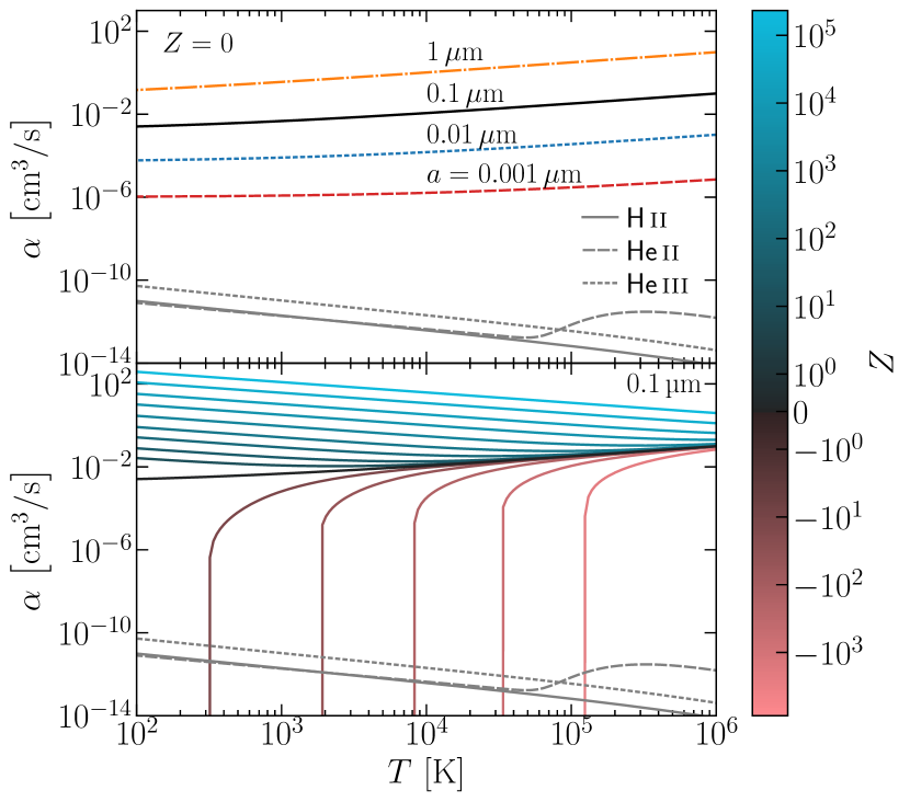
Figure 1: Electron charging rate coefficient as a function of plasma temperature for neutral grains of different sizes (top panel, indicated by the line style and colour) and for a grain of $0.1\text{\,}\mathrm{\SIUnitSymbolMicro}\mathrm{m}$ with different charge numbers (bottom panel, indicated by line colour as shown by the colour bar in symlog scale). Also shown for comparison are the hydrogen and helium recombination rate coefficients (grey lines).

In the top panel of Fig. 1 we show the electron charging rate coefficient $\alpha=J_{\mathrm{e}}/(-en_{\mathrm{e}})$ as a function of the plasma temperature for neutral grains of different sizes. Note that due to the associated uncertainties, WD01 provide identical prescriptions for $J_{\mathrm{e}}$ for both carbonaceous and silicate grains, even though in reality there likely is a composition dependence. $\alpha$ varies strongly with grain size, as expected due to the variation in the geometrical cross section. Note, however, that despite their smaller sticking coefficient, the rate coefficient for small grains is enhanced. One would expect a factor of $\sim${10}^{6}$$ between the rates for the $0.001\text{\,}\mathrm{\SIUnitSymbolMicro}\mathrm{m}$ and the $1\text{\,}\mathrm{\SIUnitSymbolMicro}\mathrm{m}$ grain, but at $100\text{\,}\mathrm{K}$ it is only $\sim${10}^{5}$$ due to the small grain effect discussed above.

In the bottom panel, we show $\alpha$ for $a=$0.1\text{\,}\mathrm{\SIUnitSymbolMicro}\mathrm{m}$$ and different charge numbers as indicated by the line colour. Hereafter, $0.1\text{\,}\mathrm{\SIUnitSymbolMicro}\mathrm{m}$ is our reference grain size as it is typical of the diffuse ISM and it will be represented by a solid black line in its neutral state. The lower limit on the charge numbers shown is set by auto-ionization (cf. WD01 Eq. (24)), while the upper limit is set by Coulomb explosion, assuming a tensile strength $S_{\mathrm{max}}=${10}^{11}\text{\,}\mathrm{d}\mathrm{y}\mathrm{n}\,\mathrm{c}\mathrm{m}^{-2}$$ for both grain materials (cf. WDB06 § 10.2.1). The auto-ionization limit for carbonaceous grains is slightly lower than for silicate grains, so it was chosen here. Positive grain charges result in a higher charging rate due to Coulomb focussing, which is more efficient for slower electrons (low temperatures). For negative charges, the rate is zero at low $T$ until the electrons have enough kinetic energy to overcome Coulomb repulsion. At this point the rate rises very steeply, soon reaching values comparable to those of the neutral case.

A similar analysis can be performed on the proton charging rate coefficient, yielding similar results as per Eq. (1); it is thus not repeated here for the sake of brevity.

2.2 Photo-electric charging

An astrophysical plasma will generally be pervaded by electromagnetic radiation, resulting in the absorption of photons by grains. Fig. 2 shows the volume-normalized absorption cross section as a function of photon energy $h\nu$ for grains represented by homogeneous spheres of graphite (top panel) and silicate (bottom panel) of different radii, computed in the Silicate-Graphite-PAH framework as described in App. A. The computation assumes neutral grains, but these values are also adopted for charged grains, since no prescription for the computation of their cross sections is available. For $h\nu<$200\text{\,}\mathrm{e}\mathrm{V}$$ and $a<$0.1\text{\,}\mathrm{\SIUnitSymbolMicro}\mathrm{m}$$, different resonances are present across grain compositions, while larger grains show a flat dependency on $h\nu$, referred to as “grey” absorption. At X-ray energies, absorption edges are visible since photons can interact with single constituent atoms. Finally, note that the increase of $\sigma_{\mathrm{a}}/a^{3}$ at $h\nu<$10\text{\,}\mathrm{e}\mathrm{V}$$ present for small graphite grains corresponds to the $2175\text{\,}\mathrm{\SIUnitSymbolAngstrom}$ extinction bump (cf. Draine 2011, Fig. 24.1).

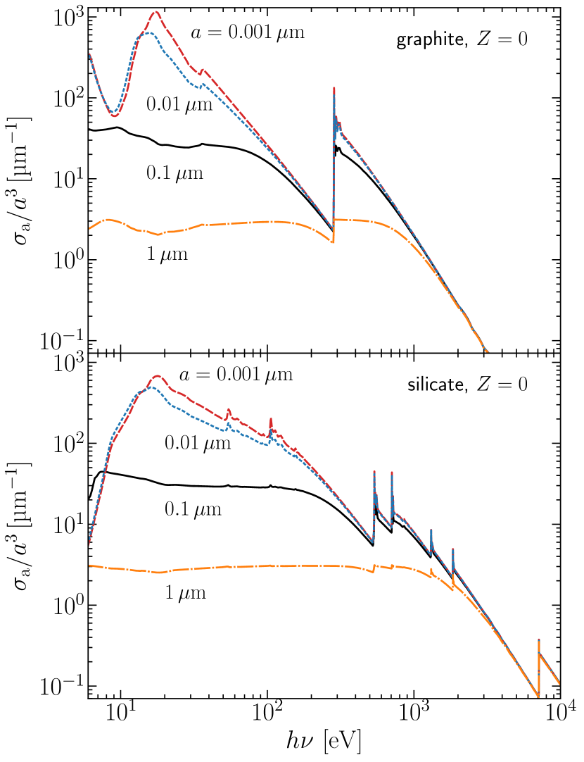
Figure 2: Absorption cross section normalized to volume for neutral graphite (top panel) and silicate (bottom panel) grains of different sizes (indicated by line style and colour) as function of photon energy.

A photon absorbed by a dust grain may eject electrons from it, thus increasing $Z$. The average number of electrons ejected following an absorption event (with a fixed set of parameters) is referred to as photo-electric yield $Y$. WD01 have computed separate yields for carbonaceous and silicate grains at low photon energies ($h\nu\leq$20\text{\,}\mathrm{e}\mathrm{V}$$) accounting for the dependence on $a$ and $Z$. Note that at these energies, electrons are ejected primarily from the band structure of a grain.

WDB06 updated the yield computation to treat additional processes occurring for $$20\text{\,}\mathrm{e}\mathrm{V}$<h\nu\lesssim$10\text{\,}\mathrm{k}\mathrm{e}\mathrm{V}$$. High-energy photons can eject electrons from the inner shells of a grain’s atoms, possibly inducing a cascade of Auger electrons if the first electron comes from a shell below the highest occupied one. In analogy to the secondary ionization process occurring in a gas photo-ionized by X-rays (see Graziani et al. 2018), photo-electrons released with high energy can themselves excite secondary electrons before leaving the grain. WDB06 provide an expression for each process and sum up all contributions to compute the total yield $Y$:

$$Y=Y_{\mathrm{band}}+Y_{\mathrm{inner}}+Y_{\mathrm{A}}+Y_{\mathrm{sec}}\,,$$ (2)

where $Y_{\mathrm{band}}$ is the band structure yield, $Y_{\mathrm{inner}}$ accounts for inner atomic shells which are not part of the band structure, $Y_{\mathrm{A}}$ is the associated Auger yield, and $Y_{\mathrm{sec}}$ denotes the secondary yield, which is computed accounting for all of the three previous yields.

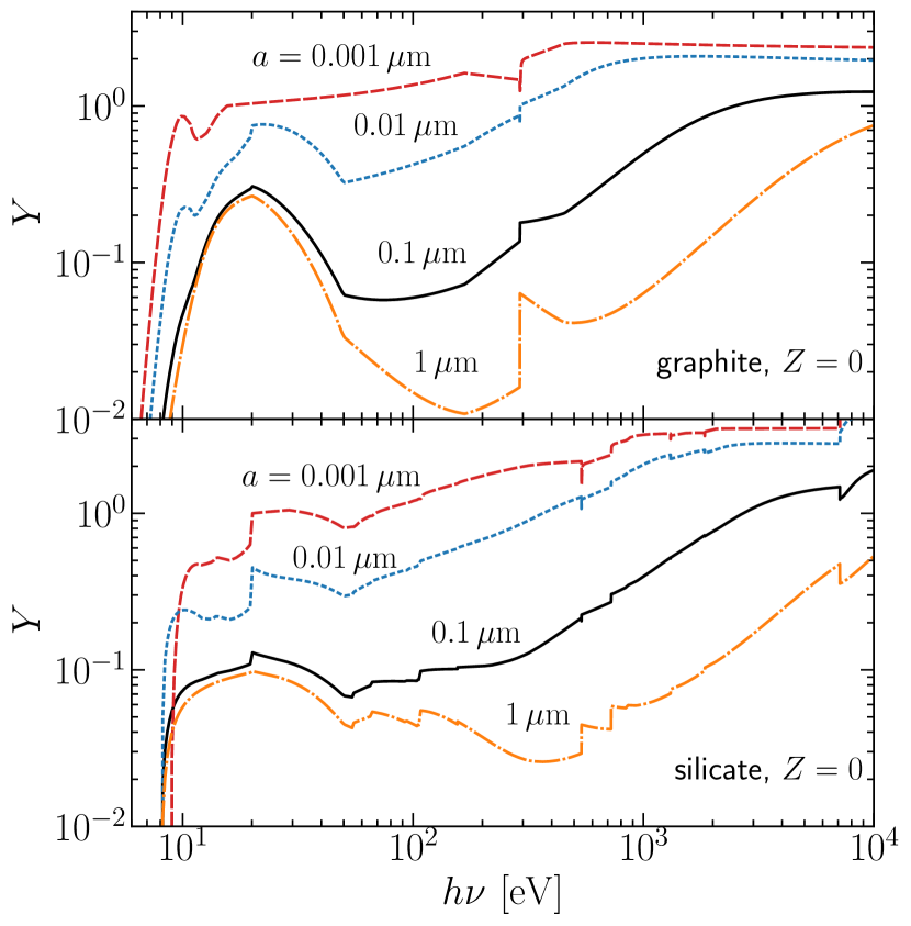
Figure 3: Photo-electron yield as a function of photon energy $h\nu$ for carbonaceous (upper panel) and silicate (lower panel) grains of various radii $a$ (indicated by line style and colour) with initial charge number $Z=0$.

Fig. 3 shows $Y$ for $Z=0$ as a function of $h\nu$, for different grain radii and materials. The yields are computed using our implementation following WDB06 (see App. C) and are tabulated in order to be included in our RT code (see § 3.1).

Grains of our reference size $0.1\text{\,}\mathrm{\SIUnitSymbolMicro m}$ (black lines) show an increasing trend up to $h\nu\sim$20\text{\,}\mathrm{e}\mathrm{V}$$ and a successive decrease until $h\nu\sim$50\text{\,}\mathrm{e}\mathrm{V}$$, where their yield starts to increase again up to X-ray energies ($h\nu\sim$\mathrm{k}\mathrm{e}\mathrm{V}$$). A strong dependence on the grain radius, concerning both trends and absolute values, is evident by comparing with other lines. Note, for example, that at $h\nu\sim$300\text{\,}\mathrm{e}\mathrm{V}$$, the value of $Y$ (for both materials) changes by a factor of $\sim$100$$ as $a$ goes from $1\text{\,}\mathrm{\SIUnitSymbolMicro}\mathrm{m}$ (big grains, orange line) to $1\text{\,}\mathrm{n}\mathrm{m}$ (very small grains, red line). For very small grains, $Y$ rapidly reaches high values, meaning that the photo-electric process is very efficient at all ionizing energies. Comparing lines with the same colour across panels, one notices also a strong dependence on chemical composition.

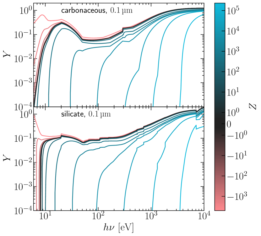
Figure 4: Photo-electric yield as a function of photon energy, $h\nu$, for carbonaceous (top panel) and silicate grains (bottom panel) of our reference grain radius $a=$0.1\text{\,}\mathrm{\SIUnitSymbolMicro}\mathrm{m}$$. Line colours indicate different values of $Z$, as shown by the colour bar (symlog scale).

The dependence of $Y$ on the initial $Z$ for our reference grain size is shown in Fig. 4. As in the bottom panel of Fig.  1, lines from red to light-blue indicate the transition from the lowest to the highest possible charge number. The Coulomb potential of positively charged grains, as expected, rapidly suppresses the photo-electric efficiency as indicated by the sudden decrease of $Y$ when $\log(Z)\geq 2$. For negative charge numbers, on the other hand, the expulsion of an electron is more likely when the incoming photons have energies $h\nu\leq$20\text{\,}\mathrm{e}\mathrm{V}$$, while at higher energies differences to the neutral case are weak. Again, a strong difference can be seen between grain materials; note, for example, that at $h\nu<$8\text{\,}\mathrm{e}\mathrm{V}$$ for very negatively charged silicate grains $Y\sim 1$, in opposition to the neutral case.

In analogy to the collisional case, given a radiation field with specific radiation energy density $u_{\nu}$, we can express the charging current experienced by a grain of some composition due to photo-ejections as follows:

$$J_{\mathrm{pe}}=e\int\mathop{}\!\mathrm{d}{\nu}\frac{cu_{\nu}}{h\nu}\sigma_{\mathrm{a}}(\nu,a)Y(\nu,a,Z)\,.$$ (3)

The excess electrons attached to negatively charged grains are assumed to occupy energy levels above the valence band by WD01. As a result, photo-detachment of these electrons has to be accounted for in the form of a separate current $J_{\mathrm{pd}}$, which is computed analogously to $J_{\mathrm{pe}}$:

$$J_{\mathrm{pd}}=e\int\mathop{}\!\mathrm{d}{\nu}\frac{cu_{\nu}}{h\nu}\sigma_{\mathrm{pd}}(\nu,a,Z)Y_{\mathrm{pd}}\,,$$ (4)

with the cross section $\sigma_{\mathrm{pd}}$ described in WD01 § 2.3.3 and $Y_{\mathrm{pd}}=1$ .

2.3 Time evolution of a grain’s charge

Not all charging currents discussed in § 2.1 and § 2.2 are relevant under all circumstances. When considering ionizing radiation, for example, $J_{\mathrm{pd}}$ is subdominant to $J_{\mathrm{pe}}$. Where a strong radiation field is present (i.e. close to ionizing sources), $J_{\mathrm{pe}}$ will also dominate over collisional charging with ions ($J_{\mathrm{ion}}$). Finally, in photo-ionized regions, where usually $T\sim${10}^{4}\text{\,}\mathrm{K}$$, $J_{\mathrm{sec,gas}}$ provides a second order contribution. For these reasons, in the discussion presented here, $J_{\mathrm{pd}}$ and $J_{\mathrm{sec,gas}}$ will be neglected. Moreover, the contribution of ions other than protons to $J_{\mathrm{ion}}$ will be neglected, i.e. we assume $J_{\mathrm{ion}}=J_{\mathrm{proton}}$.

In analogy to the case of ions (e.g. He⁰, He⁺, He⁺⁺), for a given set of conditions, a grain can be in a number of different charge states with varying probability. The associated probability distribution is referred to as grain charge distribution (e.g. WD01, Fig. 9). The number of available and typically occupied charge states, especially for large grains, however, is many times higher than in the case of ions. For this reason, we will use a simplified treatment here and consider the temporal evolution of only a single charge for given grain properties, described by:

$$e\frac{\mathop{}\!\mathrm{d}Z}{\mathop{}\!\mathrm{d}t}=J_{\mathrm{pe}}+J_{\mathrm{ion}}+J_{\mathrm{e}}\,.$$ (5)

In a steady state, the above equation becomes a root finding problem in $Z$:

$$J_{\mathrm{pe}}(Z)+J_{\mathrm{ion}}(Z)+J_{\mathrm{e}}(Z)=0\,.$$ (6)

3 The cosmological radiative transfer code crash

crash is a cosmological radiative transfer (RT) algorithm first introduced in Ciardi et al. (2001) to simulate cosmic reionization around the first stars. The RT is based on two common concepts: domain discretization and Monte Carlo (MC) sampling of the radiation field using a long-characteristics ray tracing scheme. Their combination allows to describe the radiation-matter interaction occurring in each cubic cell of a Cartesian grid, once it is crossed by a ray emitted from an arbitrary combination of sources. Both point-like sources, with arbitrary spectra (Maselli et al., 2009; Graziani et al., 2013), or a diffuse background field (Maselli et al., 2003; Graziani et al., 2019) can be chosen, depending on the astrophysical problem under investigation. crash is usually adopted to perform simulations of cosmological reionization of hydrogen and helium (Ciardi et al., 2003b, a, 2012; Eide et al., 2018, 2020) or to investigate specific problems linked to the fluctuations of the UV background at fixed redshift (Maselli & Ferrara, 2005; Graziani et al., 2019). Small scale cosmological environments, such as the ones involved by quasar H ii regions (Maselli et al., 2004; Kakiichi et al., 2017; Graziani et al., 2018) or Local Group-like volumes (Graziani et al., 2015) have been also investigated, proving the flexibility of the crash algorithm in simulating a wide range of cosmological environments.

As the general crash algorithm is extensively described in a series of technical papers (Maselli et al. 2003, 2009; Graziani et al. 2013, 2018; GCG19), here we provide the minimal outline necessary to present how Eq. (6) is solved within the time dependent RT scheme.

During the ray tracing cycle of crash, each time $N_{\nu}$ photons (distributed in a frequency bin around $\nu$) cross a cell along a cast path $l$, their number is reduced by:

$$\Delta N_{\nu}=N_{\nu}(1-\mathrm{e}^{-\tau_{\nu}})\,,$$ (7)

where $\tau_{\nu}=\sum_{i}\tau_{i,\nu}$ is the total optical depth of the cell at frequency $\nu$ and $i$ indicates the various species present in the environment, either neutral atoms, ions or dust. The partial optical depth contributed by each $i$ is given by

$$\tau_{i,\nu}=n_{i}\sigma_{i}l,$$ (8)

where $n_{i}$ and $\sigma_{i}(\nu)$ are number density and absorption cross section of the species $i$, respectively. The absorbed photons are then distributed among $i$ as:

$$\Delta N_{i,\nu}=\frac{\tau_{i,\nu}}{\tau_{\nu}}\Delta N_{\nu}\,.$$ (9)

This is used to estimate the time dependent photoionization rates for the different gas species and the associated heating contributions. Taking into account recombination, collisional ionization and various cooling processes, the ionization state and temperature of the gas are then updated by evolving the corresponding set of coupled, time-dependent differential equations (see original papers for more details). In GCG19 the energy deposited in the dust component was simply neglected and the corresponding photons removed from the total flux. In the next section we will detail how they are used in this release of the code to compute the effects of grain charging.

3.1 Grain charging implementation

In this section we describe the numerical implementation of grain charging in the latest release of crash (Graziani et al., 2018), extended in GCG19 to account for dust absorption in the hydrogen ionizing band $h\nu\in[$13.6\text{\,}\mathrm{e}\mathrm{V}$,$10\text{\,}\mathrm{k}\mathrm{e}\mathrm{V}$]$. The code version adopted here features a significant number of improvements in both algorithmic and engineering aspects, resulting, most significantly, in greatly improved behaviour when simulating media with high dust density, as documented in App. B.

To account for grain charging, we first expanded the list of initial conditions to include 3D maps of the charge at simulation start of each dust species $k$, $Z_{k}(t_{0})$. Furthermore, the DUST_SPECIES type has been extended to load tables of the electron charging rate coefficient as a function of plasma temperature and grain charge $\alpha_{k}(T,Z)$, as well as the photo-electric yield as a function of photon energy and grain charge $Y_{k}(h\nu,Z)$. The tables can be provided by any dust model, keeping the implementation general, while the data-set of built-in models has been expanded by including tables of the relevant quantities for the Silicate-Graphite-PAH model, computed as discussed in § 2. The DUST_IN_CELL type has been consistently extended to store the charge of each species in the cell.

A fully self consistent treatment of dust charging (neglecting the grain charge distribution; cf. § 2.3) in our time dependent scheme would require extending the system of equations describing the gas component by a set of equations (one per dust species) in the form of Eq. (5). Since grain charging timescales ($\sim e/(J_{\mathrm{pe}}-J_{\mathrm{e}})$, Draine & Lazarian 1998) can be many orders of magnitude shorter than hydrogen and helium ionization/recombination timescales (cf. Fig. 1), time integration of such a system is extremely challenging. The timesteps adopted in crash are adaptive, since a cell is updated every time it is crossed by a photon packet, but they are on the order of the gas recombination time scale and thus generally much longer than the dust charging timescale. Reaching small enough timesteps would require prohibitive numbers of photon packets or a complete restructuring of the crash algorithm to enable the use of implicit solvers, which are known to be difficult to combine with MCRT schemes (Noebauer & Sim, 2019). We therefore take a different approach and assume grain charges to always be in steady state at the timescales crash resolves, i.e. we evolve the grain charge of each species in each cell from steady state to steady state as the environment (radiation field, temperature, ionization state) changes.

More precisely, every time a cell is crossed by a photon packet, we compute the number of photons of each frequency absorbed by each dust species $\Delta N_{k,\nu}$ using Eq. (9). Since it is heavily affected by MC sampling noise, we accumulate this quantity over a number $N_{\mathrm{d}}$ of packet crossings ($\Delta N_{k,\nu}^{\mathrm{acc}}=\sum_{\mathrm{crossings}}\Delta N_{k,\nu}$) to obtain a robust estimate of its time average $\Delta N_{k,\nu}^{\mathrm{acc}}/\Delta t_{\mathrm{d}}$, where $\Delta t_{\mathrm{d}}$ is the time since the last charge computation. We then use a root finder to solve Eq. (6) for the new charge value $Z_{k}$, approximating the photo-electric charging current:

$$J_{\mathrm{pe},k}=\frac{e}{\Delta t_{\mathrm{d}}}\sum_{\nu}\Delta N_{k,\nu}^{\mathrm{acc}}Y_{k}(h\nu,Z_{k})\,,$$ (10)

and the electron charging current:

$$J_{\mathrm{e},k}=-en_{\mathrm{e}}\alpha_{\mathrm{e},k}(T,Z_{k})\,,$$ (11)

where $Y_{k}$ and $\alpha_{k}$ are computed by interpolation on the pre-loaded tables, and $n_{\mathrm{e}}$ and $T$ take the current cell values. $J_{\mathrm{ion}}$ is implemented analogously to $J_{\mathrm{e}}$, replacing electron properties with the corresponding proton properties. We verified that a value of $N_{\mathrm{d}}\sim 100$ is typically required to overcome MC noise. Finally, note that while we account for the dust contribution to $n_{\mathrm{e}}$, we do not yet account for the dust contribution to cooling and heating of the plasma.

A detailed validation of our approach in complex time dependent configurations is still outstanding and requires convergence tests in $N_{\mathrm{d}}$. This is particularly important in the case of very small grains, as their charging timescales could reach values comparable to those of the gas. The results presented below are not affected by the above issue, since they correspond to global equilibria of their respective configurations. Moreover, all results presented in § 4 have been validated by convergence tests in both photon sampling and ranges of assumed $N_{\mathrm{d}}$.

In GCG19, our simulations included only one dust species with properties corresponding to the average of a grain population. When considering only absorption, this does not constitute an approximation (Steinacker et al., 2013). However, since we now account also for charging, we have to resolve a given grain population in composition and size, as these strongly affect the charging process. A typical run of the updated code might now include eight dust species (see below). While accurate in terms of implementation, this is demanding in terms of memory requirements, which scale with the product of the number of computational cells, dust species and frequency bins (to compute $\Delta N_{k,\nu}^{\mathrm{acc}}$). The memory cost is especially high in cases investigating ISM environments, where the dust generally pollutes a large part of the domain, but in realistic cosmological simulations the dust-contaminated domain is usually restricted to the environments of star-forming galaxies, significantly limiting the number of enriched cells.

The new features documented above will be employed in the following to first study a series of H ii region configurations. We consider eight dust species, spanning the radii $a\in\{0.001,0.01,0.1,1.0\}\,$\mathrm{\SIUnitSymbolMicro}\mathrm{m}$$ and the compositions graphite and silicate in the Silicate-Graphite-PAH framework. We note that we use carbonaceous charging properties ($\alpha$ and $Y$, cf. § 2) for the graphite grains, since no pure graphite prescription is available.

4 Results

In this section we investigate the grain charges attained in H ii regions created by sources with different multi-frequency spectra. In all cases we assume a realistic dust population consisting of the eight species mentioned towards the end of § 3.1. Since for the time being we do not account for PAHs, we use the graphite/silicate size distribution from Mathis et al. (1977, MRN hereafter) extended down to $0.001\text{\,}\mathrm{\SIUnitSymbolMicro}\mathrm{m}$ with normalizations as given by Weingartner & Draine (2001b) to determine their relative abundances.

In detail, § 4.1 describes the spherically averaged profiles of an ideal H ii region created by a black body source, while the ideal case created by the spectrum of a young stellar population including binaries is investigated in § 4.2. In both cases, we consider only H-ionizing frequencies ($h\nu>$13.6\text{\,}\mathrm{e}\mathrm{V}$$). Finally, the grain charges obtained in a more realistic case are discussed in § 4.3, where dust, gas and stellar source distributions are motivated by a hydrodynamical simulation and the spectrum of each stellar population is modelled using BPASS (Stanway & Eldridge, 2018). In this case, we extend the spectra down to $6\text{\,}\mathrm{e}\mathrm{V}$.

4.1 Ideal H ii region of a black body source

Here we adopt the basic simulation setup of the reference run in GCG19 § 5.1 and thus only summarize its most important properties. A source with a black body spectrum ($T_{\mathrm{bb}}=${10}^{4}\text{\,}\mathrm{K}$$, and emissivity $\dot{N}=${10}^{49}\text{\,}\mathrm{s}^{-1}$$) is placed in the corner of an $($85\text{\,}\mathrm{p}\mathrm{c}$)^{3}$ box with a constant gas density $n_{\mathrm{g}}=$1\text{\,}\mathrm{c}\mathrm{m}^{-3}$$ and cosmological abundances of H and He mapped onto a Cartesian grid with $256^{3}$ cells. The medium is polluted with dust at a gas-to-dust ratio (GDR) of $124$. Initially, gas and dust are neutral and the gas temperature is $T=${10}^{2}\text{\,}\mathrm{K}$$. We run the simulation for $10\text{\,}\mathrm{M}\mathrm{y}\mathrm{r}$, ensuring that equilibrium in temperature and ionization is reached, while using $2\text{\times}{10}^{9}$ photon packets to obtain good MC convergence (to the per mill level in the volume averaged gas ionization fractions).

Fig. 5 shows the spherically averaged profiles of the charges of grains of different sizes (lines) and materials (panels) in the final equilibrium configuration. Close to the source, all grains are positively charged, but they attain negative charges as the photon flux becomes weaker when moving away from the source. At the hydrogen ionization front ($\sim$60\text{\,}\mathrm{p}\mathrm{c}$$), the number density of free electrons is drastically reduced, resulting in grain charges becoming more positive again. In contrast to the mono-frequency cases presented in App. D, however, the residual flux of high-energy photons beyond the ionization front results in weak ionization of the gas and thus a non-zero number density of free electrons, which keeps the charges negative instead of neutral outside the front. Further comparisons with equivalent simulations neglecting the contribution of $J_{\mathrm{ion}}$ also confirm that the implementation of this current is necessary when the flux of ionizing radiation is reduced significantly, i.e. at $r>$30\text{\,}\mathrm{p}\mathrm{c}$$. It is responsible, in particular, for the value of the charge to progressively approach its neutral, initial value at $r>$70\text{\,}\mathrm{p}\mathrm{c}$$. Also note that in the external regions of an idealized configuration like the one adopted here, the ionizing flux becomes so weak that numerical artefacts can affect the stability of the values when computing the spherical average for all quantities, including the predicted charge. This is the case, for example, of $1\text{\,}\mathrm{\SIUnitSymbolMicro}\mathrm{m}$ grains (orange line), whose trend starts to oscillate instead of becoming neutral at large distances. In the next section this issue will be solved by adopting a more realistic source spectrum extending to higher frequencies.

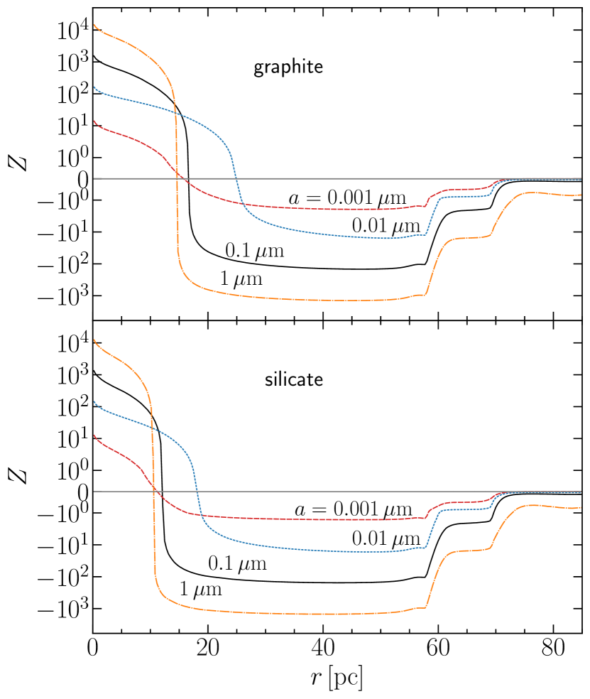
Figure 5: Spherically averaged grain charge at equilibrium as a function of distance $r$ from an ionizing black body source. The simulation includes eight species of grains with different sizes (line styles) and chemical compositions (panels). The horizontal line, corresponding to a neutral grain, is drawn to guide the eye. See text for details.

Finally note that even the highly idealized H ii region investigated here features a complex charge structure, predicting spatially strongly varying conditions for grain evolution.

4.2 Ideal H ii region created by a young stellar population

In this section we investigate a dusty H ii region surrounding a young stellar population including binary stars. The spectrum of the adopted population is obtained using pyBPASS and the BPASS v2.2.1 (Stanway & Eldridge, 2018) spectral database. A stellar metallicity of $0.1Z_{\odot}$, a Chabrier initial mass function (Chabrier, 2003) with an upper limit of $300\text{\,}\mathrm{M}_{\odot}$, a stellar age of $5\text{\,}\mathrm{M}\mathrm{y}\mathrm{r}$, and a mass of ${10}^{6}\text{\,}\mathrm{M}_{\odot}$ are chosen. The resulting spectrum is down-sampled to 100 bins for use in crash, and it extends into the soft X-ray regime ($h\nu\sim$5\text{\times}{10}^{2}\text{\,}\mathrm{e}\mathrm{V}$$), which we can consistently treat, including secondary ionization processes. The source has an ionizing emissivity $Q_{0}=$2.75\text{\times}{10}^{52}\text{\,}\mathrm{s}^{-1}$$, and is placed in the corner of a $($60\text{\,}\mathrm{p}\mathrm{c}$)^{3}$ box containing a homogeneous, cosmological H-He mixture at a density of $10\text{\,}\mathrm{c}\mathrm{m}^{-3}$ and dust at a GDR of $50$. These ISM conditions are motivated by average values found around young stellar populations, resolved in simulated dusty galaxies evolving in the epoch of reionization ($z\gtrsim 6$) in Graziani et al. (2020).

Fig. 6 shows the resulting radial profiles of the charges of grains of different sizes (lines) and materials (panels) at equilibrium. The qualitative behaviour is similar to that seen in Fig. 5, however, the harder spectrum results in higher charge values close to the source. In the $\sim$2\text{\,}\mathrm{p}\mathrm{c}$$ region closest to the source, the Coulomb explosion limit is reached for the smallest ($0.001\text{\,}\mathrm{\SIUnitSymbolMicro}\mathrm{m}$) grains of both compositions. Our numerical scheme does not account for grain destruction yet, so it simply sets the grain charge to zero in this region in order to clearly identify the possibly affected domain.As discussed in the previous section, far from the source the value of the negative charge is clearly affected by the contribution of $J_{\mathrm{ion}}$, as we also verified by comparing with a similar run disabling its contribution. Differently from the black body case, on the other hand, the presence of a soft X-ray flux at a large distance helps stabilizing the computation and removes any numerical artefacts.

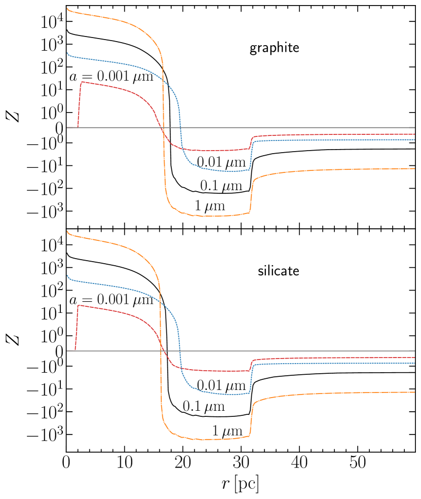
Figure 6: Like Fig. 5, but for a source with the spectrum of a young stellar population as provided by BPASS. See text for details.

The results presented here clearly show the potential of our implementation to investigate grain charging and some of its consequences as discussed in the introduction to this chapter. The case of high energy radiation causing partial gas ionization and thus making available electrons to negatively charge grains is particularly interesting, as this could be conducive to the growth of grains. Naturally, a closer investigation is required, taking into account diffuse matter and source distributions representative of the ISM, as well as further radiation bands, which could increase the photo-electric charging rate and drive grain charges towards more positive values. A first step in the direction of a more realistic model is taken in the next section.

4.3 Grain charging in a star forming region

In this section we investigate the effects of radiative transfer on the charge distribution of cosmic dust grains present in a star forming region of a galaxy evolving in the epoch of Reionization. To this aim, we set up a more realistic radiative transfer configuration which extends the previous cases by including non-H-ionizing frequencies down to a photon energy of $6\text{\,}\mathrm{e}\mathrm{V}$ and by mimicking a realistic gas distribution embedding the sources of radiation in high density, dust enriched clouds.

4.3.1 Initial conditions and cloud modelling

The star forming region under investigation is extracted from a galaxy present in a novel dustyGadget simulation (Graziani et al., 2020), which extends the rich chemical network of Gadget (see Maio et al. 2007 and references therein) by self-consistently accounting for the production of dust grains by evolving stars (Mancini et al., 2015; Ginolfi et al., 2018; Marassi et al., 2019) and their successive evolution in the galactic ISM (Hirashita, 2012). More specifically, the adopted simulation is performed on a cubic cosmological volume of $\sim$70\text{\,}\mathrm{c}\mathrm{M}\mathrm{p}\mathrm{c}$$ (comoving $\mathrm{M}\mathrm{p}\mathrm{c}$) side length with a gas/dark matter particle resolution of $\sim$8.2\text{\times}{10}^{6}$/$4.4\text{\times}{10}^{7}\text{\,}\mathrm{M}_{\odot}$$ using the feedback model introduced in Graziani et al. (2020), which is proven to guarantee a reliable estimate of the total dust mass present in the simulated galaxies. We note that although this large-scale simulation does not resolve the detailed structure of star forming regions (see below on how we address this issue), it nevertheless provides a reliable estimate of the amount of gas and dust, as well as the stellar content of such regions.

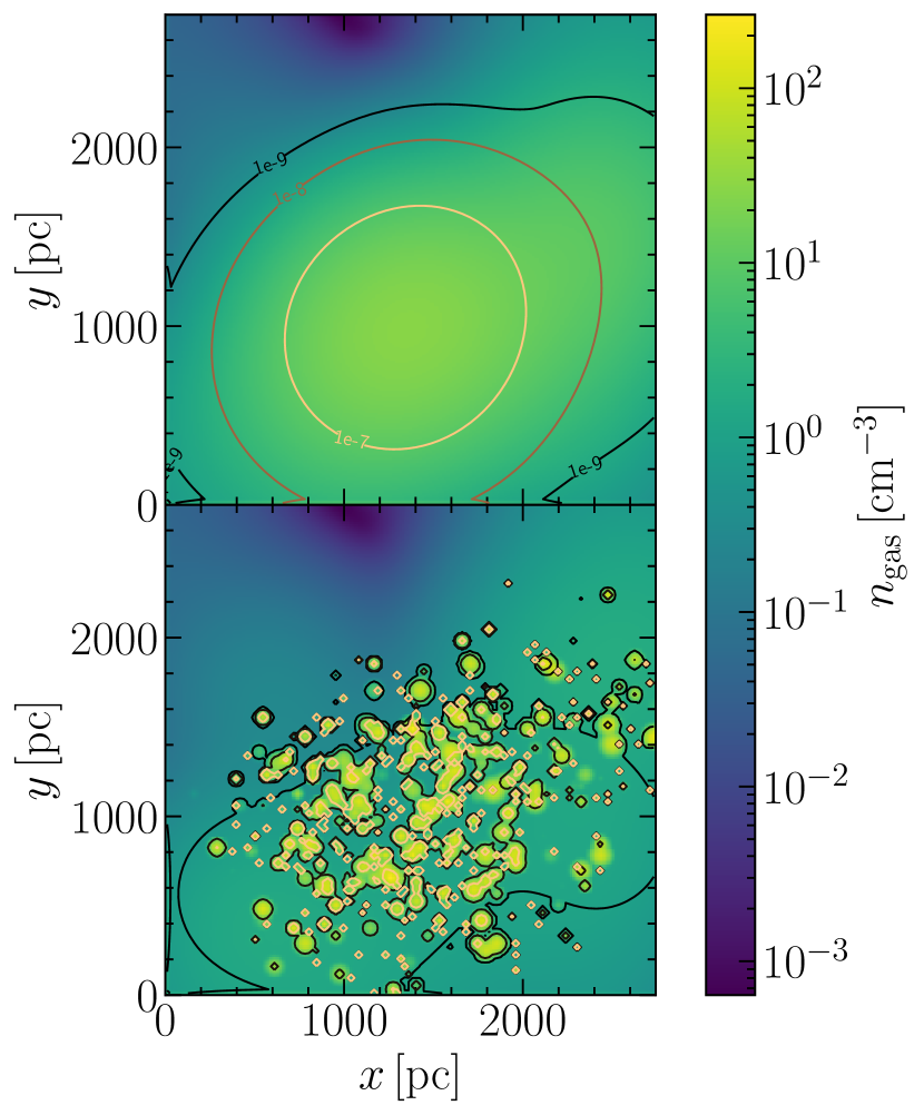
Figure 7: Slice cut of the gas number density distribution in the star forming region selected to compute grain charging, before (top) and after (bottom) remodelling of the clouds (see text for more details). The corresponding dust number density distributions [$\mathrm{c}\mathrm{m}^{-3}$] are shown using contour lines.

Here we select one of the most massive objects present in the cosmological volume at $z\sim 6.69$ and extract a cubic, isolated galactic region of $2.8\text{\,}\mathrm{p}\mathrm{k}\mathrm{p}\mathrm{c}$/side including $90$ stellar particles with masses around $2\text{\,}\mathrm{M}_{\odot}$ and ages varying from ${10}^{6}\text{\,}\mathrm{y}\mathrm{r}$ to $3\text{\times}{10}^{8}\text{\,}\mathrm{y}\mathrm{r}$. Their initial metallicity is spread over a range from $5\text{\times}{10}^{-4}\text{\,}\mathrm{Z}_{\odot}$ to $0.1\text{\,}\mathrm{Z}_{\odot}$. Their spectra in the range $6500\text{\,}\mathrm{e}\mathrm{V}$ are obtained from BPASS as in § 4.2, resulting in a spread in ionizing emissivity from $7\text{\times}{10}^{47}\text{\,}\mathrm{s}^{-1}$ to $2\text{\times}{10}^{53}\text{\,}\mathrm{s}^{-1}$. Gas and dust particles present in this region are projected onto a Cartesian grid of N${}_{\mathrm{c}}=128$ cells/side (i.e. the maximum allowed by the hydrodynamic simulation and equivalent to a spatial resolution of $21.9\text{\,}\mathrm{p}\mathrm{c}$), to create the necessary initial conditions for a crash run (see § 3 or refer to GCG19 for more details).

Fig. 7 (top panel) shows the resulting spatial distribution of $n_{\mathrm{gas}}$ in a slice cut of the volume selected to contain the brightest star. At the centre of the image, the gas number density, shown as colour palette, is $\sim${10}^{2}\text{\,}\mathrm{c}\mathrm{m}^{-3}$$ and it rapidly drops by three orders of magnitude towards the cube edges. The contour lines show the total grain number density corresponding to the adopted extended MRN size distribution. As already mentioned above, the mass resolution of the simulation is inadequate to resolve the clumpy gas structure typical of observed star forming regions. The total gas and dust mass present in the volume guarantee, on the other hand, that dust and metal pollution of the region are consistent with all episodes of star formation and evolution thanks to the accurate dust yields adopted in dustyGadget.

To address this issue and effectively increase the spatial resolution, we remodel the distribution of cold gas (see Graziani et al., 2020, for a description of the simulated ISM phases). The total mass of cold gas present in the volume is distributed among spherical clouds with a fixed density of $100\text{\,}\mathrm{c}\mathrm{m}^{-3}$ and sizes drawn from a power-law distribution with index $1.1$ ranging from $1\text{\,}\mathrm{p}\mathrm{c}$ to $100\text{\,}\mathrm{p}\mathrm{c}$. Once created, the cloud centres are distributed randomly among grid cells, weighting each cell with its original cold gas content; clouds are allowed to overlap creating even denser regions. The resulting gas distribution preserves the original gradient in spherical averages around the cube centre. The distribution of clouds and diffuse gas is shown in the bottom panel of Fig. 7 (same slice cut as in the top panel), visually illustrating how the above procedure creates an intricate pattern of overlapping clouds surrounding or embedding the stellar sources.

The dust associated with the original cold gas content of each cell is finally distributed among all clouds, weighting with the inverse of the cell-cloud distance. The resulting dust distribution is illustrated in the panel using contour lines of the grain number density; note how it statistically correlates in space with gas clumps by checking the positions of pink iso-contour lines and yellow regions present in the bottom panel. Also note that all the iso-contour lines twist together following the cloud clustering; this creates sudden spatial fluctuations of both gas and dust optical depths along different lines of sight. Large spatial fluctuations in the radiation field are thus expected, as a result of radiative transfer effects of photon filtering and shielding.

The initial temperature of the diffuse gas is taken from the hot phase of the hydrodynamical simulation, while clouds are assigned the temperature value it assumes for the cold phase (i.e. $T_{\mathrm{c}}\sim$8\text{\times}{10}^{3}\text{\,}\mathrm{K}$$). The initial charge of the grains is always setup as neutral, and the ionization fractions for hydrogen and helium are taken from collisional equilibrium calculations.

With the initial conditions described in the above paragraphs, we performed radiative transfer simulations through gas and dust and computed the grain charge distribution as described in § 3.1. The reference setup propagates ${10}^{7}$ photon packets from each source for a simulation duration of ${10}^{6}\text{\,}\mathrm{y}\mathrm{r}$ and assumes $N_{\mathrm{d}}=200$; its results are verified to be convergent by running an identical setup with photon sampling increased by one order of magnitude and testing additional values of $N_{\mathrm{d}}$.

4.3.2 Gas ionization and temperature

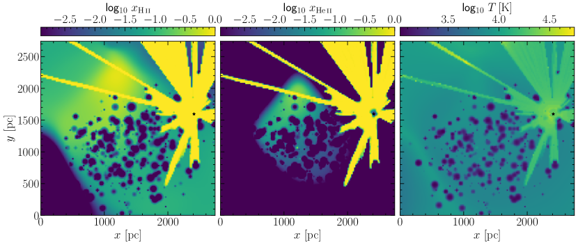
Figure 8: Slice cuts as in Fig. 7, showing hydrogen and helium ionization fractions (left and middle panel) and gas temperature (right panel) at the end of the radiative transfer simulation.

Hydrogen ($x_{\text{H}^{+}}$) and helium ($x_{\text{He}^{+}}$) ionization fractions and gas temperature ($T$) found at the end of the simulation in the usual slice cut are shown from left to right in Fig. 8. The gas close to the brightest star is fully ionized in both hydrogen and helium (yellow regions in the left and central panel). Doubly ionized helium (not shown here) is only present in direct proximity of the brightest star, where $x_{\text{He}^{+}}<1$ . While ionizing radiation can easily escape through specific lines of sight and reach the end of the simulated region (yellow pattern), dusty clouds are very effective in absorbing these photons and blocking their further propagation. In fact, even clouds close to the sources can remain significantly neutral in both H and He. The 3D picture is obviously more complicated as radiation from other sources, off the slice cut plane, and collisional ionization from hydrodynamic heating sustain a minimum fraction in ionized hydrogen and singly ionized helium. The gas temperature shown in the right panel is consistent with the ionization described above: temperatures higher than ${10}^{4}\text{\,}\mathrm{K}$ are easily found where ionizing radiation can propagate, while the densest clouds remain at the initial temperature or even lower (down to ${10}^{3}\text{\,}\mathrm{K}$). Finally note that ionization and temperature maps trace the presence of ionizing radiation only, while a background of non-ionizing photons is present in the simulated region. Its behaviour is better reflected by grain charges, as discussed in the next section.

4.3.3 Grain charges

The spatial distribution of the grain charges found at the end of the simulation is shown in Fig. 9. The figure refers to grains of radius ${10}^{-3}\text{\,}\mathrm{\SIUnitSymbolMicro}\mathrm{m}$; graphite/silicate dust is separately shown in the top/bottom panel respectively. Positively charged grains are found where the flux of radiation is high: either coming directly from the brightest source or the other, off-plane sources. Note that also non-ionizing radiation, the presence of which is not reflected by the ionization state of the gas, impacts grain charges. The figure clearly shows that dust grains can get negatively charged (green/blue regions) if located in clouds sufficiently far from the brightest source or shielded by other over-densities found along different lines of sight.

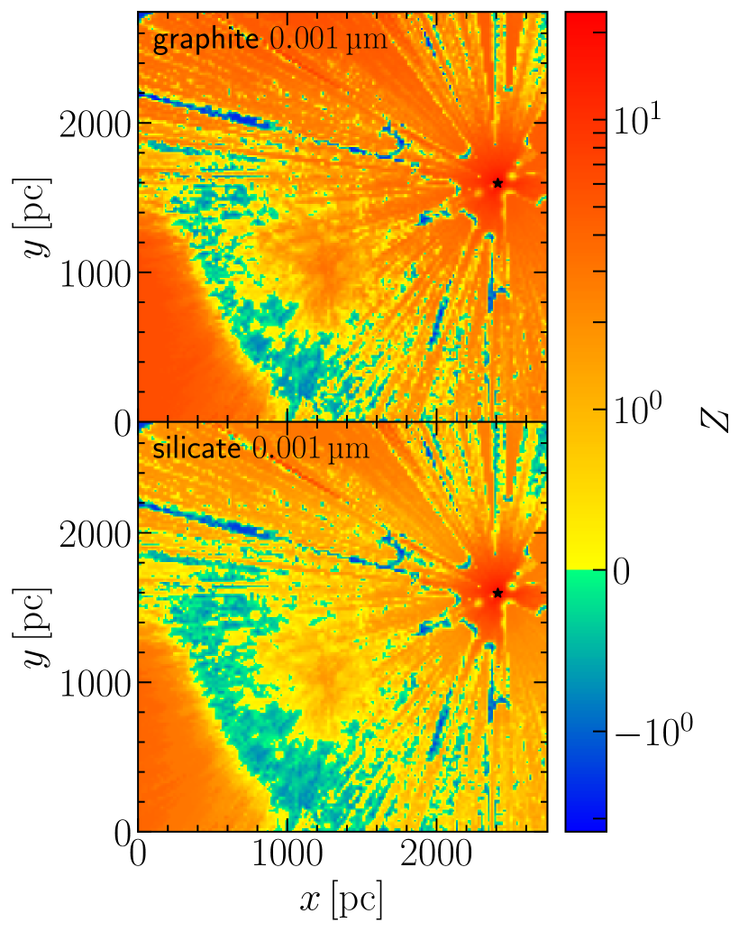
Figure 9: Slice cut of the grain charge spatial distribution in the selected star forming region. The charge of graphite grains of reference size ${10}^{-3}\text{\,}\mathrm{\SIUnitSymbolMicro}\mathrm{m}$ is shown in the top panel, while silicate dust is shown in the bottom panel. The colour palette indicates the charge acquired by grains at the end of the RT simulation: from yellow to red positive charges ($Z\geq 10$), while negative values are represented as gradient toward dark blue ($Z\leq-2$).

The potential $\Phi=\frac{eZ}{4\pi\epsilon_{0}a}$, shown in the composite of Fig. 10, is more readily comparable across grains of different sizes than their charges. By comparing the patterns, from left to right, it is clear that a negative potential (and thus charge) is favoured in the smallest grains of both chemical compositions. The graphite panels show a slightly redder tone than the silicate ones, indicating an overall slightly more positive potential for graphite grains.

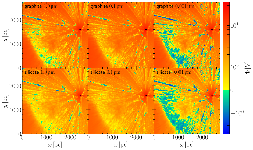
Figure 10: Slice cut of the spatial distribution of grain potential in the selected star forming region. Graphite grains are shown in the top panels, while silicate dust is shown in the bottom panels. The colour palette indicates the potential acquired by grains of different size at the end of the RT simulation. From left to right we show grains with $1\text{\,}\mathrm{\SIUnitSymbolMicro}\mathrm{m}$, $0.1\text{\,}\mathrm{\SIUnitSymbolMicro}\mathrm{m}$ and ${10}^{-3}\text{\,}\mathrm{\SIUnitSymbolMicro}\mathrm{m}$, respectively.

A quantitative picture of the statistics created in the entire volume can be found in Fig. 11, which shows the probability density (f) of $\Phi$ for the grain sizes and compositions of Fig. 10. Note that in the figure the scales and ranges of $\Phi$ are different across grain sizes. The histograms confirm the qualitative picture described in the slice cut, with distributions for graphite grains showing more weight at slightly positive potentials in the range of a few $\mathrm{V}$. At the same time, graphite grains reach lower negative potentials at any size. Negative charges are present for all grain sizes and compositions although in large grains the probability density is usually very low ($f\leq${10}^{-5}$$); the smallest grains, on the other hand, can reach potentials as low as $-5\text{\,}\mathrm{V}$ with higher values of f.

Negative charges are present with different percentage values in each grain population, strictly depending on their size and chemical composition. For example, by mass 12% of the smallest graphite grains (${10}^{-3}\text{\,}\mathrm{\SIUnitSymbolMicro}\mathrm{m}$) are negative, while the same value for silicate dust is 21%. Interestingly, the equivalent values for the largest grains are instead 4% and 2%, respectively. In this realistic case we note that the lowest values of the potential reached by intermediate and large grains are determined by $J_{\mathrm{ion}}$, which prevents values of the potential lower than $-50\text{\,}\mathrm{V}$/$-30\text{\,}\mathrm{V}$ for grains with the largest/intermediate radius. The smallest grains of both compositions, on the other hand, reach their most negative potentials as determined by auto-ionization.

Finally, it is important to quantify the percentage of negative dust with respect to the total mass. We find that at the end of the simulation (i.e. after $1\text{\,}\mathrm{M}\mathrm{y}\mathrm{r}$) about 13% of the total dust mass present in the simulated volume has a negative charge value; as expected, this is composed by silicate and graphite grains of radius ${10}^{-3}\text{\,}\mathrm{\SIUnitSymbolMicro}\mathrm{m}$ (71% and 26% respectively), with a marginal contribution of all the other larger solid particles.

Note that a non-H-ionizing galactic background/interstellar radiation field should be considered here when computing grain charges as we are considering an inner-galactic region. We defer such a treatment to future work.

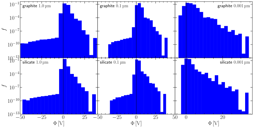
Figure 11: Probability density of the potential, $\Phi$ [V], of graphite (top panels) and silicate (bottom) dust grains at the end of the RT simulation. From left to right we show grains with $1\text{\,}\mathrm{\SIUnitSymbolMicro}\mathrm{m}$, $0.1\text{\,}\mathrm{\SIUnitSymbolMicro}\mathrm{m}$ and ${10}^{-3}\text{\,}\mathrm{\SIUnitSymbolMicro}\mathrm{m}$, respectively.

5 Conclusions

This paper introduces a novel implementation of the grain charging process in the cosmological radiative transfer code crash, extending the work of GCG19, where the contribution of dust grains was accounted for only as an additional term to the optical depth of the gas components. In this new implementation the grain charge is computed consistently with both radiative transfer effects and the assumed properties of dust grains, i.e. chemical composition and size distribution. After testing our implementation on a series of H ii regions with increasing physical realism, we studied the case of a complex star forming region extracted from a dustyGadget simulation (Graziani et al., 2020) and remodeled its cold gas phase to resolve dusty clouds. At the end of the simulation (i.e. after $1\text{\,}\mathrm{M}\mathrm{y}\mathrm{r}$) we find that $\sim 13$ % of the total dust mass remains negatively charged and largely distributed in regions far from the emitting sources or shielded by dense clouds found along many lines of sight. In particular:

• a complex distribution of grain charges is present in the entire volume with corresponding potentials varying from $-5$ to $50\text{\,}\mathrm{V}$;

• negative grains account for $\sim 13$ % of the total grain mass and are present in $18\%$ of the simulated volume at the end of the simulation; the negative mass is mainly due to silicate and graphite grains of radius ${10}^{-3}\text{\,}\mathrm{\SIUnitSymbolMicro}\mathrm{m}$ (71% and 26% respectively);

• a clear dependence on grain size emerges from the charges present in the simulated volume; a weak dependence on chemical composition is also found as graphite grains tend to acquire a slightly more positive potential while at the same time reaching lower minimal charges than silicate grains, at fixed grain size;

• grain charge does not directly correlate with gas ionization or temperature as it strictly depends on the radiation field, both at ionizing and non-ionizing frequencies ($h\nu\geq$6\text{\,}\mathrm{e}\mathrm{V}$$); negative charges seem to correlate with the distance from radiation sources, being present in both regions far from the sources or with significant shielding, as a result of radiative transfer effects.

Further investigations will be performed on zoom-in simulations of selected galaxies simulated with the dustyGadget code to establish the grain charge distribution in many environments of their resolved, multiphase dusty ISM.

Data Availability

The data underlying this article will be shared on reasonable request to the corresponding author.

Appendix A New dust cross sections

Since we encountered problems in reproducing the absorption cross sections of Silicate-Graphite-PAH mixtures using the Mie code by Wiscombe ( GCG19, Fig. 3), after the publication of GCG19 we adopted the Mie implementation used in Cloudy (e.g. Ferland et al., 2017), which provides less functionality but is also less complex. Conveniently, it applies anomalous diffraction theory in the appropriate limits ( GCG19, App. B). We extracted the relevant portions of source code and combined them into an independent C/C++ library. Moreover, we wrote a CPython extension with a NumPy universal function wrapper for the main routine, such that, after compilation, it can easily be called from Python with full support of NumPy array arguments. The code has been published.

Using this new library in combination with dielectric functions and PAH cross sections as described in GCG19 App. B, we find far better agreement with the published cross sections at all wavelengths.

Appendix B Photon counting inconsistency

We discovered an inconsistency in how ionizing photons absorbed by dust were counted in the crash version used in GCG19. This inconsistency resulted in too many photons being removed from photon packets and thus an overprediction of dust absorption. The effect is strongest in the regime of high gas densities and low GDRs, in which we reported disagreement with the analytic solution in App. A of GCG19 and which we, in light of our interest in more tenuous environments and this disagreement, avoided in the other simulations presented in GCG19. The issue has been fixed and we now find much better agreement with the analytic solution in a wide parameter range. This is illustrated in Fig. 12, where we show the hydrogen ionization fraction as a function of distance from the ionizing source normalized to the Strömgren radius, $r_{\rm S}$, for different gas densities (lines) and GDRs (panels). The analytic solution, computed as in Raga & Lora (2015), is shown in dashed and the corresponding crash results are shown in solid. The simulations were set up as described in App. A of GCG19.

We consider the agreement to be excellent, taking into account the stark differences in the two approaches. For possible origins of the remaining small deviations, see the discussion in App. A of GCG19.

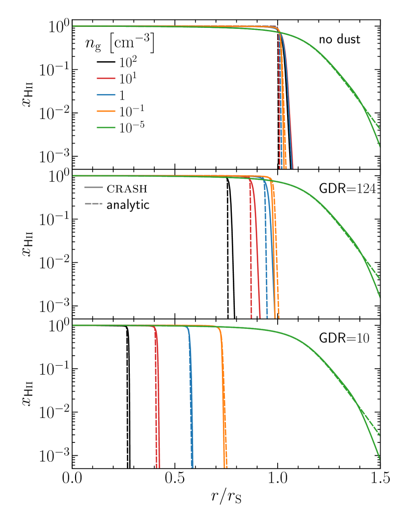
Figure 12: Hydrogen ionization fraction as a function of distance from the ionizing source normalized to the Strömgren radius for different gas densities (line colours) and gas to dust mass ratios (panels). The analytic solution (cf. Raga & Lora, 2015) is shown in dashed and the corresponding crash results are shown in solid. See text for details.

Appendix C Computation of photo-electric yields

Following WD01 and WDB06, we implemented a Python framework to compute the photo-electric yield for a grain of a given species (carbonaceous or silicate), size and charge at a given photon energy $h\nu$. Here we provide some details on our implementation, an experimental version of which has been made publicly available.

In the computation of the photon attenuation length $l_{\mathrm{a}}$ (see WD01), we use the same dielectric functions as in App. A ( GCG19, App. B) to be consistent.

In § 5, WDB06 state first that they use $E_{\mathrm{A},i,s,j}$ when evaluating the electron escape length $l_{\mathrm{e}}$ to compute $y_{0,\mathrm{A}}$ (Eq. (16)). In the next paragraph, however, they state that they use $\Theta_{\mathrm{A};i,s}$ when evaluating $y_{0,\mathrm{A}}$ and $\Theta_{\mathrm{A};i,s}$ also appears as an argument to $y_{0,\mathrm{A}}$ in Eq. (16). It is not clear to us where $\Theta_{\mathrm{A};i,s}$ could be required to evaluate Eq. (16) other than as a replacement for $E_{\mathrm{A},i,s,j}$ as the argument to $l_{\mathrm{e}}$. This would, however, effectively introduce a direct dependency of the initial Auger electron energy on the energy of the photon that created the inner shell vacancy, the filling of which initiates the Auger emission process. We do, therefore, not use $\Theta_{\mathrm{A};i,s}$ in Eq. (16) (or anywhere in our calculation, for that matter) and evaluate $l_{\mathrm{e}}$ using $E_{\mathrm{A},i,s,j}$.

When computing secondary electron yields (§ 6), WDB06 adopt bulk values for the initial energy of primary electrons ejected from band structure and inner shells (e.g. $E_{e,\mathrm{band}}=h\nu-W$) in the evaluation of Eq. (18). For consistency with the computation of primary yields, we set ${E_{e,k}=\Theta_{k}}$. This has no discernible effect on the results (see next paragraph) and is certainly negligible in light of all other uncertainties in the properties of grain materials.

In the top panel of Fig. 3, we reproduce Fig. 4 from WDB06 with very good agreement. The only difference discernible to the eye is the first peak in the $a=$0.001\text{\,}\mathrm{\SIUnitSymbolMicro m}$$ curve at ${\sim$10\text{\,}\mathrm{e}\mathrm{V}$}$. While our peak reaches $\sim 0.9$, their peak reaches only $\sim 0.7$ . This is owed to a small bug in the code that was used to plot Fig. 4 of WDB06 (J. Weingartner, private communication).

Appendix D Comparison with analytic solution

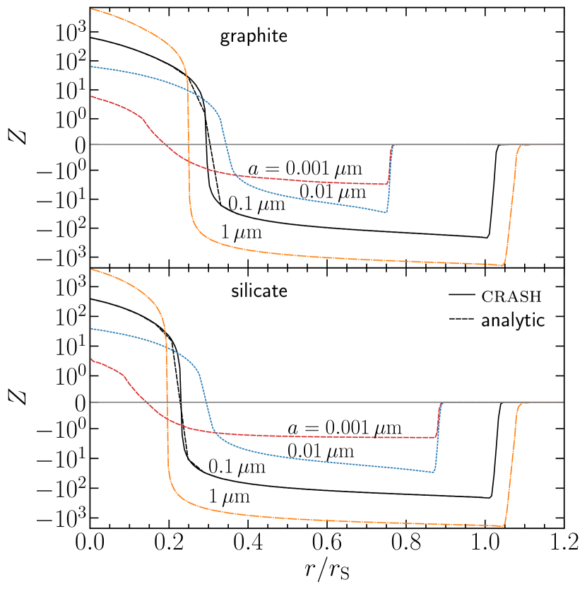
Figure 13: Grain charge at equilibrium as a function of distance from an ionizing source emitting at $13.6\text{\,}\mathrm{e}\mathrm{V}$ normalized to the Strömgren radius for simulations including grains of different sizes (line styles) and chemical compositions (panels). The gas number density is $1\text{\,}\mathrm{c}\mathrm{m}^{-3}$ and GDR$=$124$$. For $a=$0.1\text{\,}\mathrm{\SIUnitSymbolMicro}\mathrm{m}$$, we also show an analytic estimate (dashed black) for comparison to crash (solid black). The horizontal line is drawn to guide the eye. See text for details.

The analytic solution to the idealized, equilibrium dusty H ii region problem used in App. B provides the hydrogen ionization fraction $x_{\text{H}^{+}}$ and the ionizing photon flux as a function of radius from the source. While it is possible to modify it to account for dust charging (cf. Osterbrock & Ferland, 2006, § 7.7), here we take a simpler approach. For typical GDRs ($\sim$100$$), if hydrogen is highly ionized, dust charging will not appreciably change the number density of free electrons. This is clearly the case close to the source, while it is not necessarily true towards the ionization front. We therefore compute the grain charge using $x_{\text{H}^{+}}$ and the flux as given by the analytic solution, starting from the source and moving outward until we reach a point where the thus predicted charge value would result in a change of the free electron number density of more than one percent. At this point we stop the computation.

Fig. 13 shows spherical averages of the grain charge $Z$ for crash simulations featuring dust populations consisting of grains of a fixed radius (lines) and composition (panels). The simulation setup is identical to that of the simulations shown in Fig. 12 with $n_{\mathrm{g}}=$1\text{\,}\mathrm{c}\mathrm{m}^{-3}$$ and $\text{GDR}=124$, except for the fact that all dust mass is comprised of identical grains. Initially, the grain charge is set to zero and it is then evolved until equilibrium is reached. We show the analytic solution as discussed above only for $a=$0.1\text{\,}\mathrm{\SIUnitSymbolMicro}\mathrm{m}$$ so as to not overcrowd the plot.

Close to the source, the charge values are positive due to the high ionizing flux. At some distance, a transition to negative charge values takes place as free electrons from hydrogen ionization continue to be highly abundant, while the flux strongly decreases. The transition is sharper for larger grains. The charge then remains negative up to the ionization front where it returns to the initial zero value. The position of the ionization front varies depending on grain size and composition, since we keep the mass of dust constant and small grains offer a higher opacity per mass (cf. Fig. 2). The agreement with the analytic solution is excellent up to $\sim r_{\mathrm{S}}$, where we stop computing it as it is no longer valid. This is also true for the other grain sizes (not shown).

References

- Abel et al. (2005) Abel N. P., Ferland G. J., Shaw G., van Hoof P. A. M., 2005, ApJS, 161, 65
- Akimkin et al. (2015) Akimkin V. V., Kirsanova M. S., Pavlyuchenkov Y. N., Wiebe D. S., 2015, MNRAS, 449, 440
- Akimkin et al. (2017) Akimkin V. V., Kirsanova M. S., Pavlyuchenkov Y. N., Wiebe D. S., 2017, MNRAS, 469, 630
- Akimkin et al. (2020) Akimkin V. V., Ivlev A. V., Caselli P., 2020, ApJ, 889, 64
- Aoyama et al. (2018) Aoyama S., Hou K.-C., Hirashita H., Nagamine K., Shimizu I., 2018, MNRAS, 478, 4905
- Bakx et al. (2020) Bakx T. J. L. C., et al., 2020, MNRAS, 493, 4294
- Baldwin et al. (1991) Baldwin J. A., Ferland G. J., Martin P. G., Corbin M. R., Cota S. A., Peterson B. M., Slettebak A., 1991, ApJ, 374, 580
- Birnstiel et al. (2018) Birnstiel T., et al., 2018, ApJL, 869, L45
- Bohren & Huffman (1983) Bohren C. F., Huffman D. R., 1983, Absorption and Scattering of Light by Small Particles. Wiley-Blackwell, doi:10.1002/9783527618156
- Bohren & Hunt (1977) Bohren C. F., Hunt A. J., 1977, Can. J. Phys., 55, 1930
- Bouwens et al. (2021) Bouwens R., et al., 2021, arXiv e-prints, p. arXiv:2106.13719
- Casasola et al. (2017) Casasola V., et al., 2017, A&A, 605, A18
- Ceccarelli et al. (2018) Ceccarelli C., Viti S., Balucani N., Taquet V., 2018, MNRAS, 476, 1371
- Chabrier (2003) Chabrier G., 2003, PASP, 115, 763
- Chastenet et al. (2019) Chastenet J., et al., 2019, ApJ, 876, 62
- Ciardi et al. (2001) Ciardi B., Ferrara A., Marri S., Raimondo G., 2001, MNRAS, 324, 381
- Ciardi et al. (2003a) Ciardi B., Stoehr F., White S. D. M., 2003a, MNRAS, 343, 1101
- Ciardi et al. (2003b) Ciardi B., Ferrara A., White S. D. M., 2003b, MNRAS, 344, L7
- Ciardi et al. (2012) Ciardi B., Bolton J. S., Maselli A., Graziani L., 2012, MNRAS, 423, 558
- Davies et al. (2017) Davies J. I., et al., 2017, PASP, 129, 044102
- Davies et al. (2019) Davies J. I., et al., 2019, A&A, 626, A63
- Dominik & Tielens (1997) Dominik C., Tielens A. G. G. M., 1997, ApJ, 480, 647
- Draine (2011) Draine B. T., 2011, Physics of the Interstellar and Intergalactic Medium. Princeton University Press
- Draine & Lazarian (1998) Draine B. T., Lazarian A., 1998, ApJ, 508, 157
- Draine & Li (2007) Draine B. T., Li A., 2007, ApJ, 657, 810
- Draine & Salpeter (1979) Draine B. T., Salpeter E. E., 1979, ApJ, 231, 77
- Draine & Sutin (1987) Draine B. T., Sutin B., 1987, ApJ, 320, 803
- Eide et al. (2018) Eide M. B., Graziani L., Ciardi B., Feng Y., Kakiichi K., Matteo T. D., 2018, MNRAS, 476, 1174
- Eide et al. (2020) Eide M. B., Ciardi B., Graziani L., Busch P., Feng Y., Di Matteo T., 2020, MNRAS, 498, 6083
- Ercolano et al. (2003) Ercolano B., Barlow M. J., Storey P. J., Liu X.-W., 2003, MNRAS, 340, 1136
- Ercolano et al. (2005) Ercolano B., Barlow M. J., Storey P. J., 2005, MNRAS, 362, 1038
- Ercolano et al. (2008) Ercolano B., Young P. R., Drake J. J., Raymond J. C., 2008, ApJS, 175, 534
- Ferland et al. (2017) Ferland G. J., et al., 2017, Rev. Mex. Astron. Astrofís., 53, 385
- Fudamoto et al. (2021) Fudamoto Y., et al., 2021, Nature, 597, 489
- Ginolfi et al. (2018) Ginolfi M., Graziani L., Schneider R., Marassi S., Valiante R., Dell’Agli F., Ventura P., Hunt L. K., 2018, MNRAS, 473, 4538
- Gioannini et al. (2017) Gioannini L., Matteucci F., Calura F., 2017, MNRAS, 471, 4615
- Glatzle et al. (2019) Glatzle M., Ciardi B., Graziani L., 2019, MNRAS, 482, 321
- Graziani et al. (2013) Graziani L., Maselli A., Ciardi B., 2013, MNRAS, 431, 722
- Graziani et al. (2015) Graziani L., Salvadori S., Schneider R., Kawata D., de Bennassuti M., Maselli A., 2015, MNRAS, 449, 3137
- Graziani et al. (2018) Graziani L., Ciardi B., Glatzle M., 2018, MNRAS, 479, 4320
- Graziani et al. (2019) Graziani L., Maselli A., Maio U., 2019, MNRAS, 482, L112
- Graziani et al. (2020) Graziani L., Schneider R., Ginolfi M., Hunt L. K., Maio U., Glatzle M., Ciardi B., 2020, MNRAS, 494, 1071
- Hansen & Travis (1974) Hansen J. E., Travis L. D., 1974, Space Sci. Rev., 16, 527
- Hariharan et al. (2017) Hariharan N., Graziani L., Ciardi B., Miniati F., Bungartz H.-J., 2017, MNRAS, 467, 2458
- Harris et al. (2020) Harris C. R., et al., 2020, Nature, 585, 357
- Hashimoto et al. (2019) Hashimoto T., et al., 2019, PASJ, 71, 71
- Heinisch et al. (2012) Heinisch R. L., Bronold F. X., Fehske H., 2012, Phys. Rev. Lett., 109, 243903
- Hirashita (2012) Hirashita H., 2012, MNRAS, 422, 1263
- Hirashita & Inoue (2019) Hirashita H., Inoue A. K., 2019, MNRAS, 487, 961
- Hunter (2007) Hunter J. D., 2007, Comput. Sci. Eng., 9, 90
- Ibáñez-Mejía et al. (2019) Ibáñez-Mejía J. C., Walch S., Ivlev A. V., Clarke S., Caselli P., Joshi P. R., 2019, MNRAS, 485, 1220
- Ivlev et al. (2015) Ivlev A. V., Padovani M., Galli D., Caselli P., 2015, ApJ, 812, 135
- Jackson (1962) Jackson J. D., 1962, Class. Electrodyn. N. Y. Wiley 1962
- Kakiichi et al. (2017) Kakiichi K., Graziani L., Ciardi B., Meiksin A., Compostella M., Eide M. B., Zaroubi S., 2017, MNRAS, 468, 3718
- Knudsen et al. (2017) Knudsen K. K., Watson D., Frayer D., Christensen L., Gallazzi A., Michałowski M. J., Richard J., Zavala J., 2017, MNRAS, 466, 138
- Kocifaj & Klačka (2012) Kocifaj M., Klačka J., 2012, Opt. Lett., 37, 265
- Kocifaj et al. (2012) Kocifaj M., Klačka J., Videen G., Kohút I., 2012, J. Quant. Spectrosc. Radiat. Transf., 113, 2561
- Köhler et al. (2012) Köhler M., Stepnik B., Jones A. P., Guillet V., Abergel A., Ristorcelli I., Bernard J.-P., 2012, A&A, 548, A61
- Li & Draine (2001) Li A., Draine B. T., 2001, ApJ, 554, 778
- Lianou et al. (2019) Lianou S., Barmby P., Mosenkov A. A., Lehnert M., Karczewski O., 2019, A&A, 631, A38
- Ma et al. (2013) Ma Q., Matthews L. S., Land V., Hyde T. W., 2013, ApJ, 763, 77
- Maio et al. (2007) Maio U., Dolag K., Ciardi B., Tornatore L., 2007, Monthly Notices of the Royal Astronomical Society, 379, 963
- Malloci et al. (2007) Malloci G., Joblin C., Mulas G., 2007, Chem. Phys., 332, 353
- Mancini et al. (2015) Mancini M., Schneider R., Graziani L., Valiante R., Dayal P., Maio U., Ciardi B., Hunt L. K., 2015, Mon. Not. R. Astron. Soc. Lett., 451, L70
- Marassi et al. (2019) Marassi S., Schneider R., Limongi M., Chieffi A., Graziani L., Bianchi S., 2019, MNRAS, 484, 2587
- Maselli & Ferrara (2005) Maselli A., Ferrara A., 2005, MNRAS, 364, 1429
- Maselli et al. (2003) Maselli A., Ferrara A., Ciardi B., 2003, MNRAS, 345, 379
- Maselli et al. (2004) Maselli A., Ferrara A., Bruscoli M., Marri S., Schneider R., 2004, MNRAS, 350, L21
- Maselli et al. (2009) Maselli A., Ciardi B., Kanekar A., 2009, MNRAS, 393, 171
- Mathis et al. (1977) Mathis J. S., Rumpl W., Nordsieck K. H., 1977, ApJ, 217, 425
- McKinnon et al. (2017) McKinnon R., Torrey P., Vogelsberger M., Hayward C. C., Marinacci F., 2017, MNRAS, 468, 1505
- Melzer (2019) Melzer A., 2019, Physics of Dusty Plasmas. Lecture Notes in Physics Vol. 962, Springer, Cham, doi:10.1007/978-3-030-20260-6
- Mendis & Rosenberg (1994) Mendis D. A., Rosenberg M., 1994, ARA&A, 32, 419
- Mie (1908) Mie G., 1908, Ann. Phys., 330, 377
- Mulas et al. (2013) Mulas G., Zonca A., Casu S., Cecchi-Pestellini C., 2013, ApJS, 207, 7
- Murga et al. (2019) Murga M. S., Wiebe D. S., Sivkova E. E., Akimkin V. V., 2019, MNRAS, 488, 965
- Noebauer & Sim (2019) Noebauer U. M., Sim S. A., 2019, Living Rev. Comput. Astrophys., 5, 1
- Osterbrock & Ferland (2006) Osterbrock D. E., Ferland G. J., 2006, Astrophysics of Gaseous Nebulae and Active Galactic Nuclei, second edn. University Science Books
- Pierleoni et al. (2009) Pierleoni M., Maselli A., Ciardi B., 2009, MNRAS, 393, 872
- Popping et al. (2017) Popping G., Somerville R. S., Galametz M., 2017, MNRAS, 471, 3152
- Priestley et al. (2021) Priestley F. D., De Looze I., Barlow M. J., 2021, MNRAS, p. stab122
- Raga & Lora (2015) Raga A. C., Lora V., 2015, Rev. Mex. Astron. Astrofís., 51, 189
- Siebenmorgen et al. (2014) Siebenmorgen R., Voshchinnikov N. V., Bagnulo S., 2014, A&A, 561, A82
- Stanway & Eldridge (2018) Stanway E. R., Eldridge J. J., 2018, MNRAS, 479, 75
- Steinacker et al. (2013) Steinacker J., Baes M., Gordon K. D., 2013, ARA&A, 51, 63
- Tamura et al. (2019) Tamura Y., et al., 2019, ApJ, 874, 27
- Tazaki et al. (2019) Tazaki R., Tanaka H., Kataoka A., Okuzumi S., Muto T., 2019, ApJ, 885, 52
- Tazaki et al. (2020) Tazaki R., Ichikawa K., Kokubo M., 2020, ApJ, 892, 84
- Veilleux et al. (2005) Veilleux S., Cecil G., Bland-Hawthorn J., 2005, ARA&A, 43, 769
- Waxman & Draine (2000) Waxman E., Draine B. T., 2000, ApJ, 537, 796
- Weingartner & Draine (1999) Weingartner J. C., Draine B. T., 1999, ApJ, 517, 292
- Weingartner & Draine (2001a) Weingartner J. C., Draine B. T., 2001a, ApJS, 134, 263
- Weingartner & Draine (2001b) Weingartner J. C., Draine B. T., 2001b, ApJ, 548, 296
- Weingartner et al. (2006) Weingartner J. C., Draine B. T., Barr D. K., 2006, ApJ, 645, 1188
- Whittet (2010) Whittet D. C. B., 2010, ApJ, 710, 1009
- Willis et al. (1973) Willis R. F., Feuerbacher B., Fitton B., 1973, in Greenberg J. M., van de Hulst H. C., eds, IAU Symposium Vol. 52, Interstellar Dust and Related Topics. State University of New York at Albany, Albany, N.Y., U.S.A, p. 303
- Zhukovska et al. (2018) Zhukovska S., Henning T., Dobbs C., 2018, ApJ, 857, 94
- van Hoof et al. (2004) van Hoof P. A. M., Weingartner J. C., Martin P. G., Volk K., Ferland G. J., 2004, MNRAS, 350, 1330
- van Hoof et al. (2020) van Hoof P. A. M., Van de Steene G. C., Guzmán F., Dehghanian M., Chatzikos M., Ferland G. J., 2020, CAOSP, 50, 32
- van de Hulst (1957) van de Hulst H. C., 1957, Light Scattering by Small Particles. John Wiley & Sons