and CAS Center for Excellence in Topological Quantum Computation,
University of Chinese Academy of Sciences (UCAS), Beijing 100190, China
Baby universes, ensemble averages and factorizations with matters
Abstract
We investigate 2D topological gravity theories with matter fields turned on. We compute correlators of boundary creation operators with extra matter insertions. We provide a systematic procedure to determine a set of -states on which the correlation functions of the different boundary operators factorize. Our results suggest that the boundary dual is an ensemble average of theories with different numbers of replicas of a seed matter contribution that is represented by excitations on top of the gravity sector. The construction of the -states and the subsequent computations in the Hilbert space point of view are most conveniently done when the bulk couplings of the matter fields are expanded in a basis of vortices, which can be thought of as a 1-dimensional analogue of the SD-branes. We further demonstrate the existence of null states and the conditions imposed by reflection positivity. Moreover, in the CGS model with only disk and cylinder topologies we map the baby universe creation and annihilation operators to the coupling constants in the one time SYK model, which allows us to match the wormhole and half-wormhole contributions in the CGS model explicitly to those identified in the SYK model. This explicitly realizes Coleman’s initial idea. Some details of the computations in a variety of concrete models are presented.
1 Introduction
Recent advances Penington:2019npb ; Almheiri:2019psf ; Almheiri:2019hni ; Penington:2019kki ; Almheiri:2019qdq in deriving the Page curve Page:1993wv ; Page:2013dx from semi-classical gravity have partially resolved the information paradox Hawking:1976ra of black hole physics and also vastly improved our understanding about quantum gravity. A major lesson from these developments is that classical gravitational path integral is actually able to access aspects of the quantum information if other nontrivial configurations, for example the complex Saad:2018bqo ; Witten:2021nzp or constrained Saad:2018bqo ; Cotler:2020lxj saddles, non-saddle contributions Saad:2018bqo ; Stanford:2019vob , and saddles that probe the discrete spectrum of the boundary dual theory Saad:2021rcu , are included.
In particular, the wormhole saddle is perhaps the most mysterious one and has recently attracted much attention see e.g. Hebecker:2018ofv ; Kundu:2021nwp for recent reviews. Wormholes are configurations connecting remote spacetime regions. When these regions are originally connected, an extra wormhole connection can be interpreted as the creation and absorption of a baby universe. Wormholes and baby universes are quite mysterious since naively they are in tension with unitarity; information appears to lose due to the entanglement between the quantum states in the parent universe and the states in the baby universe, and physics on the different asymptotic boundaries do not factorize due to the “non-local” interaction through the wormhole Hawking:1987mz ; Giddings:1987cg ; Lavrelashvili:1987jg ; Hawking:1988ae . Resolutions of this tension are suggested Coleman:1988cy ; Giddings:1988wv ; Giddings:1988cx ; Polchinski:1994zs where the creation and annihilation of wormholes are proposed to be related to the randomness of coupling constants which are called -parameters and -states. As a result, the wormhole amplitudes compute an ensemble average of quantum theories labelled by different -parameters, and unitarity is restored in each sector. 111There are discussions McNamara:2020uza about the incompatibility between the existence of the parameters and the Swampland proposal that prefers no free parameter in quantum gravity in dimensional spacetime. For a review, see Brennan:2017rbf ; Palti:2019pca . However, this statement has not been realized in explicit computations. For example, it is not clear how to remove the enormous would-be redundancy in the naive baby universe Hilbert space.
Wormholes and baby universes lead to new puzzles Witten:1999xp ; Maldacena:2004rf when we consider AdS/CFT correspondence. The existence of multi-boundary AdS spacetime suggests the gravity theory is dual to an ensemble of theories rather than a specific theory. But this is quite unfamiliar in the previous known AdS/CFT examples. On the other hand, some low dimensional examples, such as the Jackiw-Teitelboim (JT) gravity Jackiw:1984je ; Teitelboim:1983ux , do hint at possible ensemble theories as the boundary dual. JT gravity is firstly shown Maldacena:2016hyu ; Kitaev:2017awl to describe the low-energy sector of the Sachdev-Ye-Kitaev (SYK) model Sachdev:1992fk ; KitaevTalk2 with random coupling. Furthermore, it is shown Stanford:2019vob ; Saad:2019lba that JT gravity is dual to a matrix ensemble. Later on more explicit 2d Stanford:2019vob ; Iliesiu:2019lfc ; Kapec:2019ecr ; Maxfield:2020ale ; Witten:2020wvy ; Arefeva:2019buu ; Betzios:2020nry ; Anninos:2020ccj ; Berkooz:2020uly ; Mertens:2020hbs ; Turiaci:2020fjj ; Anninos:2020geh ; Gao:2021uro ; Godet:2021cdl ; Johnson:2021owr ; Blommaert:2021etf ; Okuyama:2019xbv ; Forste:2021roo and 3d Maloney:2020nni ; Afkhami-Jeddi:2020ezh ; Cotler:2020ugk ; Perez:2020klz ; Cotler:2020hgz ; Ashwinkumar:2021kav ; Afkhami-Jeddi:2021qkf ; Collier:2021rsn ; Benjamin:2021ygh ; Dong:2021wot ; Dymarsky:2020pzc ; Meruliya:2021utr examples of ensemble duality are proposed. See further explorations of wormhole, baby universe and ensemble average in Saad:2018bqo ; Saad:2019pqd ; Blommaert:2019wfy ; Giddings:2020yes ; Benjamin:2020mfz ; Blommaert:2020seb ; Gesteau:2020wrk ; Bousso:2020kmy ; Stanford:2020wkf ; Harlow:2020bee ; Peng:2020rno ; Garcia-Garcia:2020ttf ; Goel:2020yxl ; Chen:2020ojn ; Hsin:2020mfa ; Anegawa:2020lzw ; Belin:2020jxr ; Marolf:2021kjc ; Casali:2021ewu ; Janssen:2021stl ; Cotler:2021cqa ; Verlinde:2021kgt ; Verlinde:2021jwu ; Altland:2021rqn ; Freivogel:2021ivu ; Blommaert:2021gha ; Stanford:2021bhl ; Raeymaekers:2021ypf ; Betzios:2021fnm ; Qi:2021oni ; Almheiri:2021jwq ; Heckman:2021vzx ; Blommaert:2021fob ; Ambjorn:2021wdm ; Dong:2021oad ; Engelhardt:2020qpv ; Iliesiu:2021are . The tension between Euclidean wormholes and AdS/CFT is usually referred to as the factorization problem.
In Marolf:2020xie , Marolf and Maxfield showed that the failure of factorization and dualities involving an ensemble of theories are very general for gravity theory with wormholes by studying a 2d toy model. This model is a theory of 2d topological surfaces whose partition function can be treated as a (circular) boundary creation operator . The correlation functions of the boundary creation operators can be systematically computed. They found the natural interpretation of the boundary dual of this topological gravity theory is an average of an ensemble of theories weighted by a discrete Poisson distribution. The eigenvalues of are explained as the parameters of the theory and they only take integer values. Motivated by this model, the factorization problem is studied carefully in Saad:2021uzi , where they find that (approximate) factorization can be restored if we add back the “off-diagonal” contribution which later on is called the half-wormhole. This idea is explicitly realized in some other toy models Saad:2021rcu ; Mukhametzhanov:2021nea ; Garcia-Garcia:2021squ ; Choudhury:2021nal ; Mukhametzhanov:2021hdi . Some generalizations of this model are also proposed. In Balasubramanian:2020jhl , the 2d surface is equipped with spin structures, in Casali:2021ewu the bulk theory is reduced to a 1d worldline theory, and in Gardiner:2020vjp , the bulk theory is replaced by a Dijkgraaf-Witten theory.
In this paper, we study various properties of the matter sector coupled with the topological surface theories, both that proposed in Marolf:2020xie and also the model introduced in Coleman:1988cy ; Giddings:1988cx and recently analyzed in Saad:2021uzi . We compute the correlators of boundary creation operators with matter fields turned on, and find the result can again be written as an average over boundary field theories. It turns out that there is also a version of the factorization problem in the matter sector; on the other hand, the correlators with matter fields do factorize in a refined set of -states. We propose a relatively general procedure to find those states. In some cases, it seems there are multiple choices of the -states and the different choices look quite distinct from each other. We discuss the relations between these choices and their possible consequences. We further discuss the null states in the Hilbert space of the baby universes with additional matter fields. Besides, the results we found seem to suggest that due to the matter couplings we can give some refined interpretation of the boundary dual; on each of the original -state, the boundary dual can be considered as replicas of a seed matter theory. In the matter-coupled CGS model, we analyze the factorization problem in more detail and argue that its resolution requires the field content on the “auxiliary” boundary to be correlated with the field content on the closed baby universe.
2 Review of the topological gravity theory of surfaces
Following Marolf:2020xie , we use to denote the boundary condition of circular boundaries and to denote the corresponding boundary creation operator. A general state of the theory is
| (1) |
here is the no-boundary state. The inner product is computed by a path integral subject to the boundary condition
| (2) |
where is some measure which can be understood as symmetry factors and is the bulk Euler’s character that does not count the number of boundaries. For any (connected) closed surface without boundaries, the summation equals to
| (3) |
Therefore the vacuum diagrams with different number of genera sum to
| (4) |
It is more convenient to define the normalized vacuum state . In this note, without special notice, all the correlation functions are computed within the normalized vacuum state so that the results in Marolf:2020xie are simply
| (5) |
where is the Bell polynomial.
In analogy with the AdS/CFT duality in higher dimensions, the bulk one-point function
| (6) |
is related to the partition function of the dual boundary theory. In the present case, the boundary theory should be a topological quantum mechanics with vanishing Hamiltonian therefore the value simply counts the dimension of the Hilbert space
| (7) |
As discussed in Marolf:2020xie , we should not directly identify since ; rather, the bulk results should be regarded as an ensemble average of different boundary values
| (8) |
where is considered as a random variable drawn from a Poisson distribution with parameter , and is the probability of . The natural interpretation of this result is that the boundary dual of this topological gravity theory is an ensemble average of different boundary theories with a Poisson probability measure. Indeed, this ensemble average interpretation maps the moment generating function (MGF) of the ensemble of boundary theories, , precisely to the bulk result in (5).
Furthermore, since has the physical meaning of creating a boundary, the above result indicates that we can map the ground state of each individual boundary theory with a fixed to the -states
| (9) |
of the bulk operator. The projection coefficient of this map, namely the probability distribution , provide a geometric meaning to the theory and the bulk -state; the in the probability distribution means the corresponding bulk configuration has connected components. Since these -states diagonalize the operator, then naturally counts the number of connected components of spacetime configuration.
3 Turning on topological matters
In practice, lots of interesting physics such as Hawking radiation, happen in the presence of matter fields. Therefore it is interesting to turn on bulk matters in the topological gravity/surface theory in Marolf:2020xie . In the rest of this paper, the matter theory describes particle trajectories222Equivalently one can think of these particle trajectories as topological lines. on the 2d surface. We will only consider topologically distinct trajectories that end on the boundaries of the 2d surface; these trajectories can also be interpreted as the (topological) Witten diagrams of the bulk matter theory.
3.1 Bulk computations
To set up our computation, we would like to introduce operators that create boundary excitations and shoot particles into the bulk. A naive choice is to introduce the set of matter operators , and boundaries with matter insertions would be
| (10) |
where the index labels the particle states (or species) and we define this state by inserting the operator on the boundary created by the original boundary operator .
However, we immediately notice a subtlety that
| (11) |
where is the matter operator that shoots a “particle” into the bulk from boundary and the operator creates a boundary of type . This is true because only when acts after the operator the matter can be created. This suggests that a more convenient way to deal with the boundary Hilbert space description is to not consider and as separate operators, rather, we should consider new types of boundary operators
| (12) |
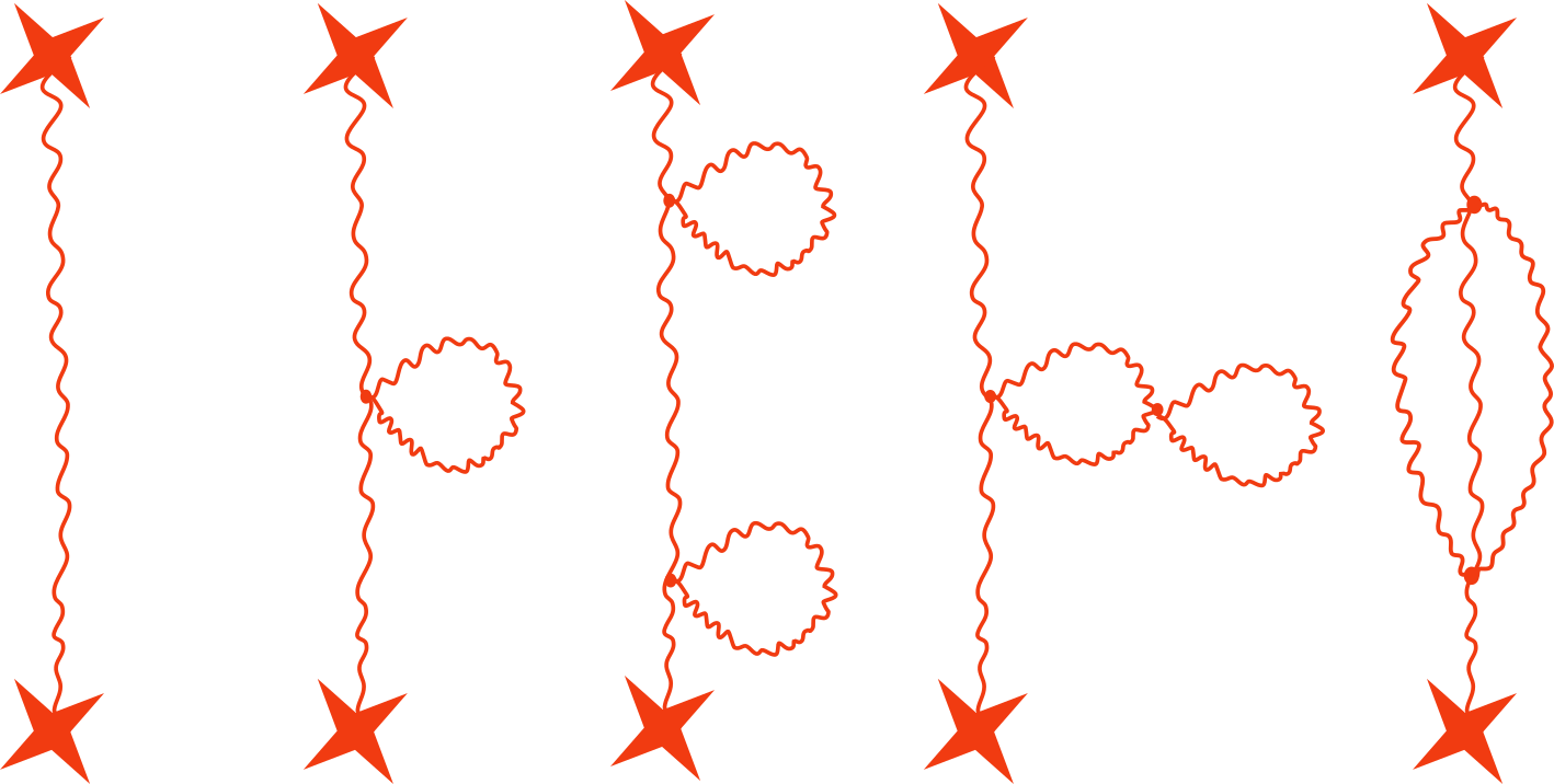
To clarify the notation, the here is quite general, it can be a single particle state or other complicated many-particle states. An illustration of this is shown in Fig. 1.
It is clear that the original “vacuum” boundary operator commutes with since they are different boundaries.
Because non-trivial topological configurations are allowed on the bulk surfaces, the propagating excitations may wind around non-trivial cycles, see e.g. Figure 2 for an illustration. In this note, we will not study this refined structure (a simple illustration of how it can be handled is shown in Appendix A). If we were studying this theory in Lorentzian signature, this omission helps forbid the presence of “closed timely curves”. However, in the following we focus on Euclidean computations, and closed curves are not strictly forbidden. Nevertheless, in this paper, we take this Lorentzian intuition as motivation and still impose the no-winding assumption for simplicity.
Notice that this assumption will not over-simplify the computation. The reasoning follows from the intuition learned from the surface computation in Marolf:2020xie : summing over non-trivial topologies amounts to renormalize the surface contribution from to . It is very likely that in the matter section this is also true; summing over the winding sectors simply leads to a renormalization of the bulk propagators. So imposing this no-winding condition is effectively equivalent to directly working with renormalized correlation functions.
We start by computing the correlation functions involving only the boundary operators, namely and . The correlation functions receive both the gravitational contributions and the matter computations.
As an illustration, it is useful to first present the calculation of a simple example , see Figure 3.
In this case we can first compute the gravity contribution, which results in two possible topologies, a pair of disks contributing and a cylinder contributing . Then on each surface, we compute the correlation functions of the matter that are injected into this surface.333The matter correlators are normalized by . Putting the two contributions together, we get
| (13) |
where the first term comes from the two-disk geometry, as shown in Figure 3(a), and the second term comes from the cylinder geometry, as shown in Figure 3(b). As a consistency check, we find the correlator (13) reduces to
| (14) |
without any matter insertion as expected. Notice that in deriving the above expression, we have neglected the backreactions of the matter fields to the background geometry. In fact, in our model both the gravity and the matter theory are topological so perturbative backreations are automatically absent. However, we do assume the matter fields are “light” and the non-perturbative backreactions can be neglected, which means we assume the insertion of bulk matter field does not change the topology of the background spacetime, pictorially this means the contributions shown in Figure 4 is not allowed.
To complete this demonstration, we evaluate the matter contribution in the above expression. The simplest choice is to consider free matter theory
| (15) |
In this theory, higher-order correlation functions of the matter fields all factorize into products of these 2-point functions. The final 2-point correlation function thus reads
| (16) |
As can be seen from this explicit example, the matter fields not only contribute a multiplicative factor, but they could also significantly alter the structure of the gravitational path integral, even if we do not consider the non-perturbative corrections from the matter fields.
Next, we move on to compute the correlation functions in a generic theory, which can be done in a few steps as follows.
First, we compute the partition function of the matter theory on a single (connected) surface with an arbitrary number of boundaries
| (17) |
where is the -point correlation function of the bulk matter theory on a connected surface, which is computed by summing over topological distinct Witten diagrams. The subscript indicates that we consider all the matter contributions on a given connected surface. For later convenience, we call the function the surface connection polynomial (SCP) of the bulk matter field.
In the second step, we compute the path integral on all possible bulk topologies that end on a given number of, say , boundaries . The result is a sum over configurations with different numbers of disconnected components, which is organized into the Bell polynomials. On each component the contribution from the matter fields can be computed from the known SCP function, or . Putting all these together, we get
| (18) |
where is the number of appearing in the partition .
The last step is to sum over these correlation functions to get the generating function
| (19) | ||||
| (20) | ||||
| (21) | ||||
| (22) |
Up to now, the derivation is fairly general and details of the matter theory are all encoded in the SCP function. In the above derivation, there are no constraints imposed on . In practice, since the function is defined on a single connected surface, it can also be formulated as the expectation value of some source term in the bulk matter field theory. We will present further details in later examples. Here we only present a most general schematic computation.
First, without the sources, we can compute
| (23) |
where is the “propagator” of the topological theory and describes the possible interactions of the theory.
Next, the expectation values of the matter fields with the sources are
| (24) |
where represents chemical potentials sourcing the matter insertions.
It is clear that the function depends not only on the theory we consider, it also depends on what are the operators inserted on the boundaries. So we denote by the SCP function for the special case where all the boundaries are for any fixed . To understand how this is reflected in the above general result, we consider the following special example as an illustration. Suppose we want to compute
| (25) |
We assume are only “gravitationally coupled” to each other, namely they can be connected by the same surface, but the matter lines do not go from one type to the other. In this case, the SCP has a special form
| (26) |
This relation is easily derived from
| (27) | ||||
| (28) |
When the fugacity of the different boundaries are different, it is easy to modify the above result to
| (29) |
Therefore in this special case, we have
| (30) |
In more general theories, the SCP does not factorize and we have to evaluate it as a whole.
3.2 The -states
We can rewrite the above result (22) into another form that clarifies the factorization problem and gives a clear hint on what are the -states in the presence of matter fields.
3.2.1 -states on which the correlators factorizes
We start with the rewriting
| (31) |
To get a better understanding of the physical meaning of the above results444Clearly, one way of understanding this result is to consider a redefined quantity (32) in which sense the computation is the same as the one in Marolf:2020xie with the only difference that the matter contribution is considered. But this does not provide more information about the factorization, -states, and the boundary ensemble average interpretation. Furthermore, the redefined constant depends on the chemical potential of the insertion and thus is not universal. Therefore in the following, we provide more instructive interpretations of the same result., we rewrite
| (33) |
where the potential and source are the same as that in (24), and the power is represented by introducing replicas.
If we can further rewrite it into
| (34) |
where the notation represents an integral over continuous components of and a further sum over the discrete values of , so that
| (35) | ||||
| (36) |
This expansion makes it clear that
| (37) |
An interesting feature is that there could be different ways to do the rewriting (36) or (37), as we will explain in more details in the following, for example (104)-(106), (124), (128), (185) and (187), choosing one particular rewriting or choosing a specific set of is simply adopting a certain set of basis of the -states. For later convenience, we first cast the results of (104)-(106), (124), (128), (185) and (187) here ( their derivation are provided in the later example sections)
| (38) | ||||
| (39) | ||||
| (40) |
In fact, among those different expansions, there is a more direct way to streamline the choice of a set of -states in generic theories. Consider a bulk theory with some topological bulk matter fields coupled, then at least perturbatively order-by-order we can compute the connected correlation functions of the matter fields. We then sum them up with the fugacity to get the effective action of their connected correlators; indeed the connected correlators can be obtained from the effective potential by taking appropriate derivatives with respect to the source . This effective potential for the matter part is dubbed the “curve connection polynomial” (CCP), , in the rest of this paper
| (41) |
where , is the connected -point correlation function of the bulk matter fields. 555In some sense the effective potential contains to all contact diagrams whose product leads to the connected correlation functions of the matter fields. This is the 1D analogue of the sum of surface theory discussed in Marolf:2020xie . Next we reorganize the series into
| (42) |
where the coefficients are related by
| (43) |
This relation can be reversed for any fixed to get
| (44) |
where
| (45) |
with being the Schur polynomial and means is absent in the list. Further notice that both the expressions should be considered as formal power series which might converge only asymptotically. But this is what we are familiar with in usual perturbative expansion in QFT.
A more subtle issue is that the inversion formula (44) depends on the choice of the cutoff ; for different the transformation coefficients are different. The physical meaning of the cutoff is the following. The cutoff is on the index of , which is also the power of . Therefore the cutoff sets up an accuracy goal so that the rewriting (42) can accurately reproduce the true result (41) up to the connected -point functions. As a result, if we want to compute up to -point correlation functions, we can use the above result for ; although the detailed transformation coefficients are different, the correlation function computed from any lead to the same result up to .
Working with the form of (43), we find simply
| (46) |
where labels the number of connected components of the matter fields and can be set to 1 if such information is not needed. According to (22), the generating function is
| (47) | ||||
| (48) | ||||
| (49) |
This means
| (50) |
where we have defined . Therefore the correlation function of the partition function is again a statistical average of a set of discrete values, which always take integer values in the different theories. 666Here the expression contains an infinite product, which in practice truncates to a finite product up to . Accordingly, the sum in the last factor also truncates to . But since the cutoff can be taken arbitrarily large, here and in the following we still keep the infinite product form of this expression.
This expression actually gives a clear indication of what is the set of -states. They should be labeled by an infinite tower of integers so that
| (51) |
The -states with different eigenvalues are orthogonal, and the -states with the same eigenvalue can be defined orthogonal via the Gram-Schmidt orthogonalization process. After this we get
| (52) |
This set of -states is determined to diagonalize only the operator. When different types of boundary operators appear in the correlation functions, we should go to a different basis of the -states so that all different boundaries are simultaneously diagonalized. In the latter case, we expect more labels in the -states. To verify this explicitly, we consider the above example (30). For each , we can follow the above prescription to get
| (53) |
Plugging this into (30), we get
| (54) | |||
| (55) | |||
| (56) |
Expanding it out, we get
| (57) | |||
| (58) |
We see that including other types of boundaries introduces another towers of integers that labels the -state (51), i.e. the -states now look like
| (59) |
We can then check that
| (60) | ||||
| (61) |
We expect that this is a general property, namely when more types of boundaries are included, more and more labels are needed to specify an -state. In particular, it should also be true for the basis.
We would also like to understand the physical meaning of the crucial change of basis (43) in the above derivation. On interpretation is to consider this as an expansion in terms of vortices that is analogues to the spacetime-D-brane (SD-brane) introduced for the surface theory in Marolf:2020xie or the eigenbrane introduced in Blommaert:2019wfy . Recall that the SD-brane is a coherent state of the boundary creation operator
| (62) |
Expanding out the SD-brane boundary condition means we consider all possible number of surfaces that can end on the SD-brane, and hence
| (63) |
And an eigenbrane in the JT gravity imposes a boundary condition on the brane that fixes an eigenvalue of the matrix ensemble. In our computation, the expansion basis plays the same role as a “SD-brane” for the matter fields, which we denote by , in the effective potential of the matter fields. Indeed, this vortex type of interaction in the effective potential allows any number of the matter lines to end on it
| (64) |
Furthermore, the value in the exponent is precisely the charge of the vortex under the rotation , and this charge is closely related to the eigenvalues of the -eigenstates. Given this, we call the expansion basis the “-vortex” basis.
Notice that this vortex only interact with the matter part; if we were to introduce a new type of spacetime D-brane where the matter line can also end on, we should consider the operator
| (65) |
But at the moment we do not need such SD-branes in our construction.
3.2.2 Hilbert space and null states with matters
To understand better the Hilbert space structure, we first consider the inner product
| (66) | ||||
| (67) |
For an arbitrary state , inner product of them can be computed by formal power series expansion and the linearity of the inner product
| (68) | |||
| (69) |
The norm of a state is easily obtained from this inner product and null states are simply defined as
| (70) |
Notice that although the -states with matter turned on are labelled by a tower of integers instead of a single integer, the condition that determines the null states is the same as that for the pure gravity Marolf:2020xie . For example, states of the form
| (71) |
are all null. Therefore there is also this huge gauge equivalence in the Hilbert space.
When there are different types of boundary insertions, it is easy to find that states of the following form
| (72) |
are all null states. An illustration of the null states is shown in Figure. 5.
In fact, there are other types of null states that are crucial in the construction of the Hilbert space. Their origin is from the interplay between different types of the different types of boundaries as illustrated in Figure 6.
To understand the origin of such null states, notice that the above results with different types of boundaries crucially depend on the assumption that they are mutually separable, namely their SCP satisfies (30). However, the existence of processes like the one shown in Figure 6 indicates . Some more details of this type of correlators is presented in section 4.3, and we will present a more thorough analysis of the null states in an upcoming publication. Here we only present a simple computation to illustrate that such null states could exist. Consider an -state that simultaneously diagonalizes the , , operators with the eigenvalues , and respectively. From our general discussion and the more careful treatment in section 4.3, we expect to take any value in . Furthermore, we assume the theory is invariant under the flavor rotation, thus the eigenvalues do not depend on the specific choice of the flavor index. We then consider operators that add “half” a boundary to the states; they have open boundary edges and should map the -states to other states in the Hilbert space. We denote the resulting states by
| (73) |
Now consider a general combination
| (74) |
Its inner product gives
| (75) | ||||
| (76) |
In the derivation, we have used
| (77) | ||||
| (78) | ||||
| (79) |
From this expression, it is clear that there exist choices of the eigenvalues of the different operators so that this inner product (76) can be zero, ie
| (80) |
The physical Hilbert space should be the naive ones divided by such null states. Reflection positivity also imposes a bound
| (81) |
on the norm of this state. The exact expressions of the norm and also the null states clearly depend on which theory we consider, we will present further model-specific results about the null states in later examples, such as in section 4.3. We will leave a complete analysis of these null states in the near future.
3.2.3 Comments on the -states
We now make a few comments about the results in the previous section.
The choice (51) and more generally (61) are only one way of choosing a set of -states, as will show momentarily, different choices of -states could be made. In those cases, clarifying the relations between these choices could lead to a deeper understanding of the computation. In particular, we could have chosen a different expansion
| (82) |
where is in some open subset of , instead of the choice of all the integers in (42). In the above computation, we choose (42) so that this set of bases is single-valued under monodromy around the origin once we continue the source to the whole complex plane. However, we could also choose the expansion in (82), a physical interpretation of this latter choice is that the bulk matter field is slightly heavier so that they backreact and could be regarded as conical singularities. The latter expansion is very similar in spirit with the expansion used in Witten:2020wvy where the bulk dual is also interpreted as conical defects. It will be interesting to study further details of this latter expansion scheme.
More interestingly, this change of basis (43) and (44) is true for any set of couplings up to the truncation we discussed above. Different values of the coupling constants change the shape of the distributions of the random variables used to label the -state.
The first implication of this result is that the choice of basis, namely the -states, are not unique; in different bases, the theory might look dramatically different, much more than what we discussed in the previous bullet point. For example, the different presentations might involve either continuous distribution (37), e.g. (38)-(40) or discrete ones (49) or (401)
Secondly, this result can be understood as a low-dimensional analogue of the RG flows in more familiar QFTs. 777An earlier example demonstrating this idea is discussed in Peng:2020rno . In the set of basis chosen in (42) and (43), all the higher point vertices are retained (again up to the cutoff ), and the result is a discrete sum. On the contrary, in the choice (37), or concretely (38)-(40), the result is an average over a continuous variable. This can be regarded as a toy version of renormalization to get a low energy effective action in the IR. Indeed, the -states in the basis (42) are labelled by a tower of integers
| (83) |
that reflects the existence of all the couplings. Notice that although the couplings might not all be independent, the labels we used to label the -states are all independent. For example, we can consider the case with and . All the ’s are generated by only one independent variable, but the integers are all independent random variables from different Poisson distributions. 888This is to say that the sources are not linearly related to each other, although there could be complicated algebraic relations among those, the labels associated with the different sources are thus treated totally independently. On the other hand in the basis (163) the -states are
| (84) |
where is a continuous variable. In this case, there is only one extra parameter to label the state, which manifests a coarse-graining process; many variables associated with the higher point couplings are “integrated out” in the sense that only a certain combination of them is used to describe the resulting IR physics.
Moreover, the result can be considered as one form of the realization of the original ideal of Giddings-Strominger and Coleman Giddings:1988cx ; Coleman:1988cy where the spacetime wormholes are introduced. One argument in their discussion, which is also widely accepted in the follow-up literature, see e.g. Marolf:2020xie ; Saad:2021rcu ; Saad:2021uzi and other related works, is that the choice of a bulk -state corresponds to a choice of boundary couplings. From the result (401) we see that if we identify the labels of the -states to be specific values of some boundary couplings, the bulk coupling is exactly the average of the boundary coupling with an extra weight factor due to the background value .
3.3 Boundary descriptions
From the above general discussion, we could deduce at least two different boundary dual descriptions of the bulk computation. Despite the quite different appearance, they describe the same physics. The fact that both descriptions come from the same bulk theory means they should be equivalent to each other.
3.3.1 Manifest replicas
We start with the result (22) and interpret it as a compound (Poisson) distribution. Consider a random variable that is a sum of different random variables
| (85) |
where each of the is independently drawn from the same distribution , namely they are i.i.d. Furthermore, the number of the number of is another random variable drawn from a distribution that does not depend on . Then the moment generating function (MGF), denoted by MG, of the compound distribution is
| (86) |
where is the fugacity that help organize all the higher order moments, and the moment generating function is defined to be
| (87) |
where is the moment. In our computation we consider the distribution to be a Poisson distribution with the Poisson parameter (hence the compound distribution is called a compound Poisson distribution), which has a moment generating function
| (88) |
Given this, if we consider the distribution that has a MGF
| (89) |
we find their compound distribution have a MGF
| (90) |
This is precisely the general result (22) we obtained previously. In particular, the gravity/surface contribution leads to the Poisson distribution of the number of copies of the matter fields; and the matter contribution provides the details of each copy in this compound Poisson distribution interpretation. This interpretation is pictorially illustrated in Figure 7.
As a consistent check, we notice that if we choose the distribution to be the constant distribution, which means we insert an identity operator and there is no extra matter excitations, whose probability distribution is a delta function
| (91) |
with a MGF
| (92) |
Then the resulting composite distribution is
| (93) |
which is nothing but the result of Marolf:2020xie once we normalize to .
This leads to a clear interpretation of our result (22). Recall that in the results of Marolf:2020xie the random variable counts the dimensions of the Hilbert space of the boundary theory which is drawn from an ensemble. It can be reinterpreted as a composite random variable
| (94) |
where each is a random variable that generate a sub-Hilbert space, and the are identical copies of the same system. When this sub-Hilbert system contains a single state , their contribution to , in other words, the MGFx is always . This corresponds to the distribution function in the above discussion.
While in our theory with matter fields, the effect of adding bulk matter does not change the fact that is still a trace of some sub-Hilbert spaces and the number of such sub-Hilbert spaces is still from the same Poisson distribution. These are determined by the “surface/gravity” sector of the theory, and including different numbers of replicas of the sub-Hilbert spaces leads to the ensemble of theories. However, due to the existence of the matter fields in the correlators, the sub-Hilbert that is detected contains more states due to the matter excitations; in the compound distribution language, this means the variables follow another distribution instead of the constant distribution. Our computation provides another explicit example, with matter fields coupled, of the recent insight that gravitational path integral might be dual to the average of an ensemble of field theories. Notice that ideas similar to this compound Poisson distribution have previously been discussed in Peng:2020rno although the discussion there is mainly from the field theory considerations, the interpretation in this section is closely related and inspired by Peng:2020rno .
Also notice that there could be other variance of this boundary interpretation where again the matter theory and the gravity sector play different roles. We will provide some discussions about this in section 4.4.
3.3.2 Manifest -states
The above approach makes a clear separation of the gravity contribution and the matter contribution, in particular, it manifests the replica structure of the matter sector in a given state.
There is yet another point of view where the matter and gravity contributions are combined into a new type of boundary insertion (12). Along this line of thought, the natural description is actually in terms of the eigenstates of (or the common eigenstates of and ), which we refer to as the -states in the previous section.
This leads to another boundary interpretation that is manifestly dual to the set of -states. 999Notice that in both the two points of view, the boundary dual of the bulk gravity computation are all ensemble average of theories; although they are written in different “bases” and manifest different properties.
Recall that in the approach in Marolf:2020xie the value can be interpreted as the trace of the identity operator in the boundary dual theory and hence can be identified with the dimension of the Hilbert space. Our computation (51), (61) shows that the eigenvalues of the operators contain an infinite set of integers, and their weighted sum, which is again an integer, should be considered as the trace of the inserted matter operator. Notice that unlike the previous compound Poisson distribution interpretation, here the range of the summation does not depend on explicitly and each random variables are all drawn from independent Poisson distribution; information of the specific matter coupling , and the eigenvalue of the gravity sector , are all encoded in the set of Poisson parameters. This is in sharp contrast with the previous interpretation where the composite variable is a sum of random variables whose distribution could be of different types, the explicit type of the distribution encodes the information of the matter theory and the value comes in explicitly as the number of boundary replicas.
As briefly discussed in the previous section, in this Hilbert space interpretation, if we make a very naive analogue to a collection of harmonic oscillators, these discrete values can be thought of as the eigenvalues of a set of number operators on the Fock space of the matter field; indeed, the form
| (95) |
of the eigenvalue resembles the mass square of string states where is the eigenvalue of the number operator at level and in (49) is similar to a classical action.
Concretely, we can consider a set of harmonic oscillators and , so that
| (96) |
In terms of this set of oscillators, the operators is identified with the number operator
| (97) |
as desired.
In this -state picture, the natural interpretation of the boundary dual is a collection of theories whose parameters, such as the coupling constants, are related to the labels of the -states, i.e. the set of ’s. The ensemble average is done according to the product Poisson distributions in (50), (58).
Some other choices of the -states also have clear physical meanings. For example, we can choose the sets of -states as in (104), (105), (106), and (148) (151), which are labelled by continuous variables. Different from the above interpretation of the ’s as the eigenvalues of the number operators, we can think of the as eigenvalues of some position operator in the harmonic oscillator analogue. We plan to provide a more detailed analysis of this relation in the near future.
When there are different classes of boundaries, as discussed in section (3.2.2), we just introduce multiple flavors of the oscillators and the latter computation is in exact parallel. While there could be extra subtleties/novelties in this case since by now we have considered the different types of boundaries independent. However as we discussed previously, due to the existence of the process as shown in Figure 6, there might be other relations between the different boundaries and hence extra null states other than those discussed in (72) must exist. We will provide further details of this analysis in a future publication.
3.4 Matter contributions to and
In the discussion of Marolf:2020xie , one condition imposed on the bulk path integral computation is that we should include a factor of for each of the boundaries. It is explained in Marolf:2020xie that this condition can be considered as the consequence of reflection positivity.
In the presence of matter fields, they contribute to the entropy and . For our topological theory, this comes from the contribution from the matter lines winding around the non-contractible cycles due to the genus or the boundary. Since it is clear that such winding contributions are identical on each cycle, it is clear that their contributions to and are identical. Therefore this is consistent with the condition imposed previously. In fact, if there are no other contributions, our above argument provides different reasoning of the origin of the condition .
4 Example: Real scalars
In the following, we denote the boundary operator as , where we drop the index that labels the different boundaries and keep only the index that labels different matter fields. Furthermore, in this section we focus on the simplest case where , that creates a single real particle, which is dubbed a “singleton”.
4.1 Free fields, singleton insertion
In this case the boundary insertion is .
4.1.1 Summing over diagrams
In the current case of free matter theory with singleton insertions, only even insertions lead to non-vanishing contributions. In the presence of insertions, the trajectories are simply a collection of propagators. Since the total number of such diagrams is and each diagram simply contributes a factor of , we therefore have
| (98) |
Plugging this into (17), we get
| (99) |
As expected, in a free scalar theory, the SCP is Gaussian. We then have
| (100) |
4.1.2 Bulk path integral
As discussed in general in the previous section, there is a systematic way to compute the SCP on a given surface. Since only a single surface is involved, this counting is the same as computing the partition function of the matter fields. Furthermore, since the matter field is topological, the path integral to get the partition function is simple to evaluate.
In the current free theory, the SCP is nothing but the expectation of the sources . For example, the insertion of means we turn on the source and in the free theory the expectation value of this is
| (101) |
This reproduces the previous result we got from counting all the diagrams.
4.1.3 Probability interpretation and -states
To look for the set of -states, we consider the rewriting
| (102) |
Then we get
| (103) | |||
| (104) |
We can further do a change of variable to get
| (105) |
Another useful change of variable is and we get
| (106) |
Although the most conservative point of view on this result is that the integral over should be interpreted as a probability distribution that we average over. However, if we take the point of view discussed in section 3.3.1 more seriously, we can regard the integral kernels, for example the in the last line above, as an effective action of the matter fields, once we condition on the state. Adopting this point of view, the expression (104) and (106) suggest the boundary dual to be an average over different theories with different actions; the action explicitly depends on the random variable . However, we find there exist other rewriting (105) where it seems the dual is a single theory with path integral kernel , and the average is on the operator inserted in the single theory, like the discussion in Pollack:2020gfa ; Belin:2020hea ; Peng:2020rno . This could be regarded as a proof of concept example illustrating one scenario where an ensemble average of theories could be traded for an average over an ensemble of operators/states in a single theory.
4.1.4 Multiple flavors
In this case the boundary insertion is . A direct counting leads to the simple result
| (107) |
The result is almost identical to the result in the previous case with only one flavor since the theory is free and different flavors do not mix.
One can also verify this by computing the expectation value from the following explicit integral
| (108) |
The generating function can again be written as
| (109) | ||||
| (110) |
4.2 Free fields, doubleton insertion
As we mentioned the matter operator can be quite general rather than just a single-particle state. The generating function clearly depends on the different matter insertions in the boundary theories. In this section, we consider the case with a doubleton insertion, namely , so the new boundary operator is .
4.2.1 Summing over diagrams
To compute the generating function
| (111) |
we first compute the CCP . Assuming that the theory is again free, we find
| (112) |
with the generating function
| (113) |
The corresponding SCP is
| (114) |
It can be recognized as the generating function of Wishart distribution . The first few moments are
| (115) | |||
| (116) |
Therefore following our general discussion we can obtain the generating function for the boundary operator
| (117) |
Because the matter field is free, namely the bulk matter lines do not join or split, and also because each insertion is a doubleton, we expect the result to be identical with the result of the topological surface theory with end-of-the-world branes in Marolf:2020xie . It is clear that our result indeed agrees with the result in Marolf:2020xie .
4.2.2 Bulk path integral approach
We can also compute the function from the integral of the topological matter theory
| (118) | ||||
| (119) |
Notice that in the last line we have used the fact that the normalization is
| (120) |
where is the number of flavors and it normalizes the numerator to
| (121) |
This reproduces the above result
| (122) |
When there is only one flavor, we can rewrite the generating function to
| (123) | ||||
| (124) |
Notice that in the last line we have written the integral in a manifestly positive manner. 101010Curiously, we can introduce a number of fermions/Grassmann variables to rewrite the result into (125) When there are multiple flavors, ie , in this case the is an matrix. We can thus rewrite
| (126) | ||||
| (127) | ||||
| (128) |
where is a matrix.
4.3 Free fields, singleton and doubleton insertions
Let us combine the three boundary operators which we have studied in the previous sections together and consider
| (129) |
where for simplicity we only consider one flavor of matter. The SCP is still given by summing over diagrams that are restricted on a connected surface:
| (130) |
Recall that is just the SCP of so (130) implies that is independent of and while and are correlated. The correlation can also be understood from Figure 6. Therefore the proposal (58) and (59) are not valid anymore 111111It is easy to check there is no solutions for if we naively follow the discussion around (30) or (46) since clearly the assumption (30) does not hold here. Since decouples let us focus on
| (131) |
whose CCP can be written as a double series
| (132) |
Following the idea of (42), we rewrite the CCP as
| (133) |
with the relationship
| (134) |
The inversion with the truncation still works, but the result is not very illuminating so we omit them here. Similar to (49), the generating function can be expand to
| (135) |
Therefore the -states are labeled by the tower of integers satisfying
| (136) |
Given these -states, one can also define the “half-circle” excited states
| (137) |
Let us consider the following special state
| (138) |
where there is only one non-vanishing quantum number . The norm of this state is then given by
| (139) | |||||
whose minimal value is at
| (140) | |||
| (141) |
Therefore the state
| (142) |
is null. More generally when more quantum numbers are non-zero, the null states are
| (143) |
The null condition (143) could be put into a more instructive form
| (144) |
where the notion “” indicates that the above expression (144) is true when acting on simultaneous eigenstates of the different boundary creation operators.
More generally, the above null condition gives the border of the region allowed by reflection positivity. This bound imposed by reflection positivity
| (145) |
indicates that quantum numbers of the boundaries with a lower number of insertions lead to a lower bound on the quantum numbers of the boundaries with a larger number of insertions.
Clearly, similar null states exist once we turn on boundaries with higher numbers of matter insertions, and the half-circle Hilbert space is spanned by
| (146) |
The reflection positivity also leads to relations among the quantum numbers in the set of -states that diagonalize the new set of boundary operators. In practice, the null states and the reflection positive region can be determined from the Kac determinant, or equivalent the determinant of the Hankel matrix whose elements are
| (147) |
From the familiar Kac determinant argument, or equivalently from the Hamburger theorem, the following two statements are equivalent
-
1.
The Hilbert space is positive semidefinite.
-
2.
All Hankel matrices are positive semidefinite.
Therefore vanishing of the determinants gives the null states and the positivity of minors of the above matrix gives the reflection positivity constraints. Notice that this is the same technique used in recent amplituhedron/positive geometry discussion Arkani-Hamed:2020blm .
4.4 Some further speculations about the boundary interpretation
Following the approach discussed in section 3.3.1, we can focus on a single state. Each individual boundary theory is defined in one of such -states. The matter theory is treated perturbatively, which means the inclusion of the matter fields does not affect our choice of the -state. In this interpretation, the sum over in (148)-(151) should be considered as a sum over different -states, i.e. averaging over different theories. The integrals in or are just the path integral of the matter fields within the individual theory.
To see this more clearly, we first rewrite the result more instructively as an integral weighted by an effective action. Immediately we find that the effective action does not only depend on the choice of the -states , it also depends on the choice of the operator/boundary conditions. As we have worked out in details in the previous sections, we have
| (148) | ||||
| (149) | ||||
| (150) | ||||
| (151) |
where we have defined , and notice that in both the above expressions, the integration variable and play a similar role as the boundary dual of the matter theory we coupled in the bulk.
Therefore, the exponent of the integrand should be identified as the action with the specific source inserted. Indeed, in the variable the action looks like the Liouville theory at for (149) or for (151) where is identified as the Liouville field. The insertion is also in the form of (half of) the Liouville potential. Alternatively, in the variable the action contains a logarithmic potential as in the Coulomb gas model.
One peculiar feature of this computation is that naively since the effective action is independent of the boundary insertion, it should be universal for all different types of boundary insertions. However, from our result it appears that the effective action needed to reproduce the bulk computation for the different boundary insertions are slightly different. For example, the difference between (149) and (151) is just the choice of the boundary insertions versus , or equivalently versus . However, the effective actions for the boundary matter field are different in the same -state. This is slightly counter-intuitive but it could actually be possible, viewed from both the boundary and the bulk points of view. From the boundary point of view, the effective action of the correlators is the Legendre transformation of the original theory in the presence of the operator insertions where the latter is treated as a source. So if the sources are different, the resulting effective actions after the Legendre transformation are expected to be different. From the bulk point of view, changing the boundary operator insertion has the effect of both changing the matter fields shot into the bulk and possibly changing the bulk propagator due to different boundary conditions. Indeed, as we observed here that changing the boundary insertion from to , ie from (148) to (150), the change of the effective action is simply replacing to or in the Liouville theory analogue changing to , this is the low-dimensional analogue of reducing the propagator by a factor of since the term in Liouville gives precisely the propagator of the Liouville field .
Let us reiterate here that the results on the RHS of (148)-(151) should be considered as boundary results, following the suggestion originated in Marolf:2020xie , although the LHS of the equation is computed from the bulk. This is thus a baby version of the holographic duality.
4.5 Interacting fields, singletons insertion
In the presence of interactions, it is very tedious to sum over all diagrams in the bulk and compute the SCP. However, for some simple interactions, we can compute the bulk path integral explicitly.
4.5.1 Bulk path integral approach
The simplest example is the theory with a bulk interaction. The path integral with the source turned on is
| (152) |
For simplicity, we first consider the case with only one flavor, ie . In which case the integral reduces to
| (153) |
In this case, we can evaluate the integral by expanding the coupling
| (154) | ||||
| (155) | ||||
| (156) |
where
| (157) |
We can compute the effective action from this “partition function”; it is formally just the log of the function. While we do not have a closed-form expression for it, we can find an expansion of the effective action order by order
| (158) | ||||
| (159) |
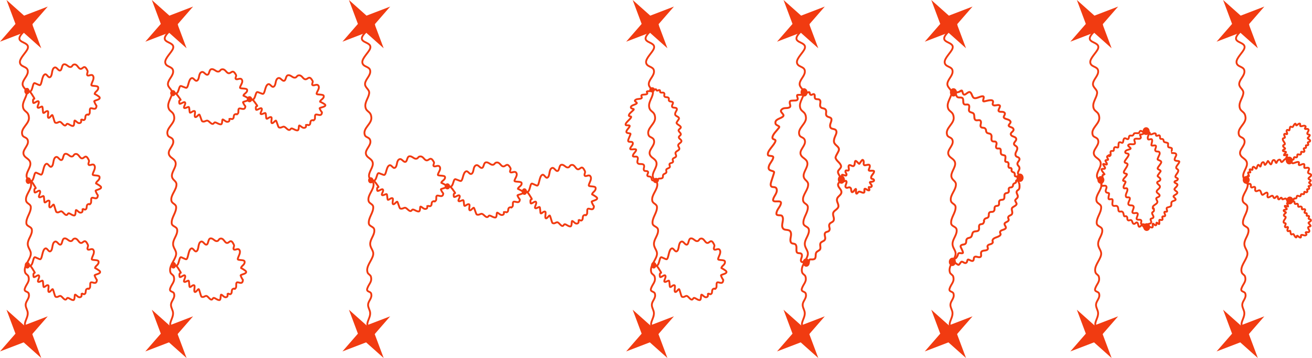
As a consistency check, the series reproduce the diagrams from perturbative expansions; for example, the terms in the order can be obtained by summing over the following diagrams in Figure 8 with the appropriate symmetry factor.
However, at this moment getting a similar expression of is not easy. To proceed, we make some simplifying assumptions. In the following two subsections, we take two of such simplifications.
4.5.2 Interacting matter fields, singleton insertions, universal coupling constants, without internal propagators
First, we consider the diagrams with only contact interactions. This can be regarded as taking the limit
| (160) |
where is the original set of couplings and the are the rescaled couplings. Further notice that the limit where we only consider the contact type diagrams is the exact 1D analogue of the 2D surface theory in Marolf:2020xie after the genera are summed over. In this limit the curve connection polynomial (CCP) is
| (161) |
To write down the generating function in a compact form, we can further assume some relations among the couplings, one choice is
| (162) |
then the generating function is
| (163) |
The corresponding SCP is
| (164) |
With these results, we get the generating function
| (165) |
Notice that in this analysis we have kept explicitly the and as free parameters. They turn out to be useful knobs that help probe different limits that we are interested in. For example, to get back the classical limit of Marolf:2020xie , we can use the 1-point vertex to terminate the boundary matter insertion and remove the effects of the matter insertion. The “propagation” of the matter can be removed by formally tuning the “self-energy” so that it cancels the bare propagator. Then setting , we arrive at
| (166) |
which is the same as in Marolf:2020xie once we normalize .
In addition, we can also probe the Gaussian limit, also known as the CGS limit. The crucial point is that we can use the free propagators between the boundaries to select only cylindrical background geometries and turn off the higher coupling by setting . Then a limit leads to
| (167) |
This is the generating function of the CGS model Saad:2021uzi .
Next, we look for the probability distribution interpretation. To achieve this, we consider the to be MGF of some random variable . One interpretation is that has two components
| (168) |
where the moment generating function of and are respectively
| (169) | ||||
| (170) |
Thus the PDF of the and variable is
| (171) | ||||
| (172) |
The probability distribution of is thus
| (173) |
where we have rewrite the Poisson probability distribution function in a continuous fashion
| (174) |
Plugging in the PDF of the normal distribution
| (175) |
we get
| (176) | ||||
| (177) |
which is again a continuous distribution. This can be considered as a superposition of different normal distributions centered at integer spaced values.
One can check this probability distribution indeed leads to the MGF (164) or (196)
| (178) | |||
| (179) |
Plugging in , and , we get
| (180) |
The probability distribution is thus
| (181) |
Making use of this result, we rewrite the partition function
| (182) | |||
| (183) | |||
| (184) | |||
| (185) |
This leads to
| (186) | |||
| (187) |
where
| (188) |
From this result, we find the correlation can again be understood as an average over a Probability distribution. A crucial difference is that now there is a second Poisson distribution due to the inclusion of the matter field; the parameter of the second Poisson distribution is proportional to , which is entirely a consequence of the inclusion of the matter field.
To understand of the appearance of the second Poisson distribution let us consider the special case with and then becomes exactly the generating function of Poisson distribution. The corresponding matter theory has universal coupling in the sense that for all we have
| (189) |
namely all the connected correlation functions are equal. Then the partition function is
| (190) | ||||
| (191) |
This means
| (192) |
Writing in this way, we tempt to conclude that the eigenvalues of the operator is , which indicates the -state can be labelled by , i.e. . The average value of this eigenvalue does not only depend on the free parameters , and of the theory, it also depends on the “dummy” variable via
| (193) |
This is an explicit example of our previous general discussion, and the proportionality to is consistent with the other interpretation that the surfaces provide different ground states and the matter fields create extra excitations on each of the ground states. Furthermore, the expansion discussed in (42) automatically truncates in this case due to the fine-tuning of all the coupling constants .
To show that our analysis is general and does not depend on this choice, we can consider another situation where the coupling constants are
| (194) |
This leads to the generating function
| (195) |
The corresponding SCP is
| (196) |
The remaining computation can be carried out in exact parallel, and the final result is the same as (185) with replaced by .
4.5.3 Interacting matter fields, singletons, tree level with internal propagators
We can in fact relax the constraints in the previous section to allow internal propagators, and thus exchanged diagrams. This leads to the tree approximation of the matter theory.
We take the -vertices to be diagonal in the flavor space and set the fugacity . As a result, matter with different species gets decoupled. For each connected component of a tree level Witten diagram, we have
| (197) |
where represents the number of external points and represents the number of -point vertices.
Notice that the number of 2-valent vertices can be shifted away by the redefinition of the edges
| (198) |
which is another equivalent expression of the fact that a theory with only 2-pt vertices is essentially free. Therefore in the following, we restrict the sum to run from 3 to infinity. The solution of this set of equations is
| (199) |
Namely, for a given set of external points and the number of internal vertices, the total number of edges and the number of one type of vertices are determined. Notice that we have also used the no-loop assumption to cutoff the sum; in the absence of loops, a connected diagram can involve only up to -valence vertices.
Then each diagram gives a contribution to the partition function as
| (200) |
where we do not put in the information of since it is totally determined by the powers of and .
In fact, for a diagram with a set of labelled vertices, there are
| (201) |
For our cases the internal vertices are not labelled, so the actual number is
| (202) |
One can compute the total number of tree diagrams for a given number of external points, these numbers have a generating function
| (203) |
where is the principal branch of the product logarithm function.
The curve connection polynomial which is associated with connected tree is a refinement of the above numbers
| (204) | |||
| (205) |
The generating function of this series of polynomials can be worked out
| (206) |
where a subtle issue is the shift by one in the expansion of the generating function. To cure this shift, we can simply integrate the generating function to get
| (207) | ||||
| (208) |
In the free limit this reduces to , which is the only contribution from the free theory.
Then the surface connection polynomial which compute moments can be computed as
| (209) |
where represents all the partitions of the integer , represents the number of times the value appears in the partition and is the length of the partition. For example, we get
| (210) | |||
| (211) | |||
| (212) |
The generating function of the surface connection function is thus
| (213) |
The full generating function is then
| (214) |
As a first consistency check, we find that at , this result reduces to the free theory result. This partition function again can be understood as a compound Poisson distribution. The moment generating function of each individual distribution is
| (215) |
This leads to a probability interpretation of the -pt correlation function
| (216) | ||||
| (217) |
where in the second line we have used the explicit expression of (213). In fact, this is a general result since the function in similar discussions will always has the form of exponential of times the generating function of the curve connection polynomial. Therefore in this step we can trivially always evaluate the -term in the expansion by replacing by .
Therefore, we get
| (218) |
As in the previous cases, in the probability interpretation the different terms in the ensemble (ie different choice of ) is just the same copy of but with extra weighting factor multiplied on . We expect the to appear here since by definition it counts the configurations among different boundaries. The only non-trivial effect is the “uniform” entrance of the rescaling factor in . As we explained in the case of free theory, the reason for this is that gravity makes replicas of the matter theory. But clearly we notice that is not the power of some polynomial so this is not the basis where the correlation functions factorize. To get to that basis, we need to go through the procedure discussed in section 3.2.1.
As another consistency check, let us derive these results again from a saddle point calculation that automatically extracts out the tree level results (213).
| (219) |
The saddle points are obtained by solving the equation
| (220) |
It turns out that there are infinite many solutions
| (221) |
where is branch of the Lambert W function or the product logarithm. Assuming that and are real values then only and are real functions. Among them the principle branch has a convergence radius and can be extended to all complex plane with a branch cut. So we claim that is the only physical saddle. This then leads to the saddle point answer of the generating function
| (222) |
which matches (213) exactly.
Another simple example is the case with only 3-pt vertices. This is the same as rearranging -array trees to binary trees. To get an explicit result, let us assume . Then the counting (197) gives
| (223) |
The number of diagrams with 3-valent vertices is
| (224) |
The curve connection polynomial is a refinement of the above numbers
| (225) | |||
| (226) |
with the generating function
| (227) |
The corresponding generating function of the surface connection polynomial is
| (228) |
We can again verify this result from a saddle point computation. Keeping only the three-vertex, the momentum generating function should be given by
| (229) |
The saddle points are easily found to be
| (230) |
However the saddle point does not obey the boundary condition that requires regularity as , so the only physical saddle is . Substituting into the integrand of (229) leads to tree-level results (228). Expanding (228) with respect to one can find
| (231) |
in the coefficient of the term reflects that there are three ways to combine two 3-vertices into a 4-vertex. After introducing 3-vertices satisfies a new distribution whose moment generating function is given by (228).
4.5.4 More general discussions
We can turn on more general types of vertices that mixes the different flavors. As a warm up, let us first consider two-valent vertices, or 2-vertex for short. We consider 2-vertices of the form . Since perturbatively correlation functions can be obtained from the source term
| (232) |
we first compute the expectation value of the source in the free theory by a simple Gaussian integral
| (233) |
Similarly we can compute the generating function (99) in the presence of 2-vertex interaction
| (234) |
As expected, two-vertices modifies the propagator from to . As a consistency check, one can compute the two-point function directly by summing over the perturbative results
| (235) |
Next we move on to a theory with three-vertex and as what is done previously we first focus on tree level results. First considering the curve connection polynomial that counts the different ways of connecting marked points on boundaries so that they are all path-connected into one component. It is straightforward to write down the first few examples
| (236) |
and more generally
| (237) |
Here the factor counts the number of ways to connect three-vertices into a tree. The result can be proved by induction. Assuming there are ways to connect three-vertices to form a tree. This tree will have edges, so there are ways to add another three-vertex. Therefore there are ways to connect three-vertices to form a new labelled tree. It will be convenient to define the generating function of this polynomial as
| (238) |
Based on this we can define the “surface connection polynomial” that counts the different ways to path connect the marked points on the boundaries of a given surface. Notice that here the different boundaries might not be path-connected, they only need to be connected by the surface and the paths among the marked points on the different boundaries could have different disconnected components. So we introduce a fugacity 121212We use the same here as the number of species because later when we consider the diagonal coupling these two numbers indeed coincide. to keep track of the number of connected paths. This polynomial can be computed for each given by definition
| (239) |
where represents all the partitions of the integer , represents the number of times the value appears in the partition and is the length of the partition. By switching the order of the summation we can find that its generating function is given by
| (240) |
As we argued above this tree-level result should be able to be reproduced from a saddle point approximation of the integral
| (241) |
from the boundary theory. The saddle point equation is
| (242) |
which is a set of non-linear algebraic equations. One can solve it order by order with respect to . For example, the first order solution is
| (243) |
In this order the saddle point approximation of (241) is
| (244) |
which in consistent with (240).
4.6 Interacting fields with flavors, doubleton insertion
We can also consider the case where the boundary insertion is a doubleton. We can get the result by evaluating the following integral
| (245) |
Notice that here we have normalized the expectation value so that .
We can expand the above expression to get
| (246) | ||||
| (247) |
where the minus signs in the above expressions are due to the coupling in the action. The second equality of each line is simply an expansion in powers of that counts all the loop expansions. We can verify this expansion order by order in the perturbative expansion of with the Feynman propagator , vertex and appropriate symmetry factors.
We can consider other generalizations where multiple flavors of matter fields coexist in the bulk. Then the path integral in the bulk can be computed as
| (248) |
To proceed, we make a change of variable
| (249) |
and the measure becomes the standard -sphere
| (250) |
For spherical symmetrical integrand, the angular part simply gives
| (251) |
and the integral reduces to the 1-dimensional one
| (252) |
The partition functions can then be computed as
| (253) | ||||
| (254) |
We can now compute
| (255) |
Expanding out the different powers we get
| (256) | ||||
| (257) |
| (258) | ||||
| (259) |
With all these results, we proceed with no difficulty to get the -state and the probability interpretation.
5 Example: complex scalars
We can also couple complex matter fields to gravity. The structure is largely the same as the results in the real scalar case, although the detailed counting is slightly different.
5.1 Free fields, singleton insertions
We consider single-particle excitation that is described by the new boundary operators and . For a free theory, all correlation functions factorize into products of 2-point functions
| (260) |
Note that and appearing in a correlation function commute because they correspond to different boundaries. We want to compute
| (261) |
One way to proceed is to do a formal power expansion
| (262) | ||||
| (263) |
where we have defined . In the first line we have only kept the even power since the odd power terms have vanishing expectation values, and in the second line we have used the fact that since there is one insertion on each boundary, the path between different boundaries are all pairwise connected and thus the counting of surfaces is the same as counting of the pairing of the matter fields. More general surfaces must be connected by such pairs, so the number of surfaces with boundaries is just different ways of connecting pairs and hence . The origin of the universal factor comes the number of ways to group and into pairs.
Alternatively, we can find CCP to be
| (264) |
where pairs of the boundary insertions are connected by paths and is the Kronecker delta function. The factor of 2 is there because ultimately we want to compute the correlation function (261) so the contains one contribution like and another factor like .
They have a generating function
| (265) |
Notice that the generating function is computed in terms of pairs of boundaries. This also indicates the generating function of SCP
| (266) |
which is also counted in pairs of boundaries. So in the expansion there is a factor in
| (267) |
The other factor is the different ways of grouping the insertions in pairs. This gives the generating function (263). In fact, for the current case, we can directly count the SCP (the surface connection polynomial)
| (268) | |||
| (269) |
where selects boundaries to have insertions and the counts the different ways of pairing up the ’s with the ’s. The remaining computation is the same as above.
From this result we can try to extract the boundary dual of our bulk computation in the matter sector. For this we adopt the statistic interpretation developed in section 3.3.1. The SCP (266) can be understood as the MFG of some random variable and satisfying the complex Gaussian distribution as expected
| (270) |
To evaluate the integral we can use the standard field redefinition
| (271) |
Accordingly (263) can be understood as the generating function of compound random variables and
| (272) |
where still satisfies Poisson distribution and satisfy the complex Gaussian distribution.
5.2 Free fields, doubleton insertions
Let us denote the interesting boundary operator by . To compute the generating function
| (273) |
we first compute the curve connection polynomial . Given the rule (260) one can easily find
| (274) |
whose generating function is
| (275) |
Therefore the generating function of the surface connection polynomial is
| (276) |
We can also include the operator into the computation
| (277) |
which is consistent with the generating function with EOW branes Marolf:2020xie once we set . The generating function (277) can be again obtained from exponentiate the connected surface connection generating function, the factorial structure of it makes sure that the result after the exponentiation gives the correct counting of the degeneracy. This means
| (278) | ||||
| (279) | ||||
| (280) | ||||
| (281) |
where the represents the surface connection polynomial with fugacities that correspond to the matter part, the and boundaries respectively. In the third line we have expressed this polynomial as products of the “mattered” boundaries and the normal boundaries with the associated symmetry, together with the defined in the expansion of (276) with respect to .
To evaluate (281), we change variable
| (282) | ||||
| (283) | ||||
| (284) |
where in the last step we have done the two sums separately since they decouple.
5.3 Interacting fields, singleton insertions, with internal propagators
To illustrate some subtleties about the interacting theories, let us study two-vertex first. The most general two-vertex is of the form
| (285) |
Note that the first two terms are not common in a complex field theory since they break the symmetry. In our theory, they will introduce non-trivial propagators (two-point function) and . The last term can be absorbed into the kinetic term and renormalize the bare propagator. So we will only consider the first two types of vertices, and do the integral to get the partition function
| (287) | |||||
Now we add in the interactions perturbatively. We focus on three-vertices of the following four types
| (288) |
A closed-form expression for the partition function of this interacting theory is complicated. Here we only provide some perturbative analysis. For example, the leading order correction is simply given by
If we focus again on the tree-level diagrams, their contributions to the partition function can also be obtained from a saddle approximation of the integral
| (290) |
The saddle point equation can be solved exactly, but the expression of the solution is very complicated so we only present its series expansion with respect to the couplings
| (291) | |||
| (292) |
Then the tree diagram contributions to are
| (293) |
Other -vertex can be analyzed similarly. The results are not very illuminating so we skip all the details.
5.4 Interacting fields, singleton insertions, without internal propagators
Another limit that is under analytic control is to consider again only contact diagrams, as we did in section (4.5.2) for the real scalar theory. One choice is to assume all the couplings to be the same, i.e.
| (294) |
whose generating function (CCP) is
| (295) |
which factorizes and hence it means that and can be counted independently.
Another choice is to consider only those preserving the symmetry
| (296) |
In this case the corresponding CCP generating function is
| (297) |
5.5 Interacting fields, doubleton insertions
From the result in the previous section, it is clear that the operators and have to come in pairs for the correlation functions to have more interesting results. So it is more natural to consider the insertion of the boundary operator . In the simplest setting, let us fix the boundary operator to be diagonal and consider the bulk vertices to be homogeneously -valent
| (298) |
For simplicity in counting the contributing Witten diagrams, we represent the two types of fields by white () and black () dots. Next we count the connected diagrams. Denoting , the numbers of external white and black points, and , the numbers of internal vertices. Because the propagator connects with , a simple counting leads to
| (299) |
where is the total number of edges. This gives
| (300) |
Furthermore, looking only at the black and white dots separately, each edge connects one and only one white/black dot, therefore we get the following refined conditions
| (301) |
This enables us to solve in terms of the external points
| (302) | ||||
| (303) |
Moreover, since the number and are integers, we get the condition
| (304) |
which requires
| (305) |
From this counting, it is clear that each diagram contributes
| (306) |
to the final partition function. There are some further simplifications that we can take.
First, we can focus on tree amplitudes, since the effect of all the loop corrections is some extra renormalization factors.
Second, we do not need to consider all types of vertices; our theory is topological and all higher valence vertices can be resolved into 3-valent vertices connected by internal propagators. As a result, we only include 3-vertices (298).
It turns out that it is still complicated to discuss the most general case with these interactions. Therefore in the rest we consider a perturbative treatment that includes at most one and one insertion. The cases without any insertion have been discussed previously, in the following we only sum over diagrams with one pair of insertions.
Again, we first consider the CCP in the presence of one pair of interactions, we get
| (307) |
Notice that comparing to the free piece,
| (308) |
we find . Then the SCP can be obtained as
| (309) |
where the product over means only one of the in the series should be kept. Explicitly, this means in terms of we have the following expansion
| (310) |
where
| (311) | ||||
| (312) |
We can then compute their generating function
| (313) |
Since this is a perturbative expansion, to the leading order we can express the above result in a more compact way
| (314) |
where
| (315) |
This means the probability distribution changes from to . This is as we expected since the inclusion of the bulk interaction should alter the boundary theory as well as their probability interpretation.
The spectral partition function is now
| (316) |
More concretely, we can expand the above MGF of the compound distribution into
| (317) | ||||
| (318) | ||||
| (319) | ||||
| (320) | ||||
| (321) |
where is the Pochhammer symbol. This means
| (322) | ||||
| (323) | ||||
| (324) |
In particular, for the result can be written as
| (325) |
Since this is only a perturbative result, we can reorganize the terms into a more suggestive manner
| (326) | |||
| (327) |
which, to the leading order of , is the same as the previous result but it is written in terms of factors.
On the other hand, we know there is another presentation of the result following the general discussions in section 3.2 where on each -state the result becomes the power of the eigenvalue. It is interesting to further understand the relation between the two presentations.
6 The operator approach in the CGS model
The theory discussed above involves surfaces with arbitrary genera. One can also study similar problems in the CGS model Coleman:1988cy ; Giddings:1988cx that only picks up the contributions from the disk and cylinder contributions. Besides the apparent simplicity of the surfaces, another property that becomes quite handy is that there is a powerful operator approach of the theory which helps streamline many of the computations. In the following, we first discuss an attempt to understand the problems we discussed above in terms of operators in the surface gravity theory, and then introduce the CGS model with its operator presentation.
6.1 Factorization and normal ordering in the surface model
In the surface model Marolf:2020xie , the correlation function does not factorize
| (328) |
in particular
| (329) |
From the bulk point of view, the non-factorization is due to the inclusion of wormhole contributions in the correlators. From the boundary point of view, it is because that the boundary theory is the average of an ensemble of theories.
We can also understand the non-factorization of the surface theory from a point of view of operators. As suggested in Marolf:2020xie , one can think of that acts as a number operator on the Hilbert space of a harmonic oscillator such that
| (330) | |||
| (331) |
The no-boundary state then can be identified with the coherent state
| (332) |
In this description, the non-factorization of can be attributed to the fact that is not normal-ordered. Suppose alternatively if we define as
| (333) |
then the factorization is manifest
| (334) |
However, the correlation functions of the normal ordered operator are not directly computed by a Euclidean path integral. In addition, there is not a universal way to define “normal-ordering” in a classical gravity theory.
It is interesting to further explore the normal-ordering effect of the boundary creation operators. For example, an interesting question is if there is a way to compute quantities like directly from bulk gravity path integral. In the following, we discuss a similar question in the CGS model introduced in Coleman:1988cy ; Giddings:1988wv and recently re-analyzed in Saad:2021rcu ; Saad:2021uzi . We will defer more detailed discussions somewhere else.
6.2 Lightening review of the CGS model
Recall the moments in the surface theory in Marolf:2020xie is given by the Bell polynomial, whose generating function can be written as
| (335) |
If we keep only the first two terms in the above sum and neglect all the other higher-order terms, then becomes approximately like the moments of a Gaussian distribution with mean value and variance being . Physically, this means we only include the spacetime with disk and cylinder topology in the theory. The model in this limit is precisely the CGS model.
In the CGS model, has a continuous spectrum and it has a natural representation as (shifted) position operator in a harmonic oscillator Hilbert space
| (336) | |||
| (337) |
The basis is orthogonal such that
| (338) |
and state are interpreted as the “-universe” states. Then the states can be expended in terms of the -universe states up to . For example the state is given by
| (339) |
Let us consider the -point function in an arbitrary state
| (340) |
where it is written as an overlap between the state and the unnormalized auxiliary state . The -point function in general does not factorize into , but it does factorize in the so-called -states which are the eigenvectors of the operator i.e.
| (341) |
Therefore the factorization equation of this correlation function
| (342) | |||
| (343) | |||
| (344) |
leads to the identity dubbed as the “exclusion rule” Saad:2021rcu
| (345) |
One can also introduce different species of boundaries , into the CGS model. In the presence of multiple species, the above exclusion rule can be generalized to
| (346) |
which is enough to guarantee the factorization of the two point function
| (347) |
6.3 Normal ordering in the CGS model
It is very suggestive to interpret as a partition function of a theory without average and similarly is interpreted as the averaged partition function
| (348) | |||||
| (349) |
Defining the “normal-ordered” quantity
| (350) | ||||
| (351) |
we find
| (352) | |||
| (353) |
and using Cyl, we get
| (354) |
Noticing that
| (355) |
we find the identity (345) or (354) are reminiscent of the half-wormhole saddle point explored in a simplified SYK model Saad:2021rcu , see also Mukhametzhanov:2021nea , where is the wormhole saddle and correspond to the half-wormhole saddle that averages to zero.
6.4 Matching (half-)wormholes in the CGS model and the SYK model
From the boundary point of view, the bulk wormhole saddle point is due to an average over an ensemble of boundary theories. A natural question is then what, if exists, is the bulk dual description of the individual theory in the ensemble. In Saad:2021rcu , this question is analyzed in a simplified SYK model at one time point, and a key finding is that if we consider the correlation function of the partition function of the SYK model, there are additional half-wormhole saddle points in addition to the wormhole saddle point. The crucial point is that the wormhole saddle is self-averaging so is still visible after we take the average over the SYK coupling, on the other hand, the half-wormhole saddle point does not survive the average and is not visible in the averaged theory. We can try to demonstrate the half-wormhole saddles in the CGS model.
In addition, the CGS model originates from the attempt to understand the effects of spacetime wormholes on quantum field theories. There the coupling constants in the field theory are considered as the expectation value of the baby-universe creation operators. It is therefore natural to ask if we could use the CGS model to understand possible effects related to the wormholes. The one time SYK model turns out to be the simplest field theory to test these ideas. In particular, this means the partition function of the one time SYK model might be rewritten into
| (356) |
where we have identified the coupling constants by a pair of baby universe creation and annihilation operators and the dots represent other terms that are left out in the CGS approximation). As a result, schematically we can write the Lagrangian of this theory as
| (357) |
which is in the form of Coleman’s effective Lagrangian to include the wormhole effects.
To proceed, consider the CGS model with species, there are thus independent Gaussian operators satisfying
| (358) |
Let us map the shifted operators to non-overlapping -element subsets of , where , and are all integers
| (359) |
Each operator, either or , satisfies normal distribution with zero mean and a finite variance. The total number of independent is , which is set to be the same as the number of species. One can give a canonical ordering of the set of , which is carried through from the ordering of the index set
| (360) |
Then together with the canonical ordering of there is a one-to-one map from Disk to the operator .
With these operators one can construct a new operator defined by
| (361) |
where the prime in the summation means it runs over non-intersecting sets of only. This operator is precisely the partition function of the SYK model at one-time Saad:2021rcu if we identify the set of to the set of coupling constants there.
From the above canonical mapping, this also defines an operator
| (362) |
In an -state of the operator in the bulk, the one-point function is
| (363) |
which could be mapped to the partition function once we identify the -eigenvalue with the corresponding value of the coupling constant . From this mapping from to the boundary partition function, we understand that the should be considered as a boundary creation operator where on the boundary it creates a copy of this SYK model resides. The fact that this boundary operator is different from the original CGS boundary means there are now at least two types of the boundaries; each operator creates a “parent” boundary dual to the SYK model and each original operator, which is now identified with the coupling constant of the SYK model, creates a baby universe/wormhole from the parent universe. This is consistent with the fact that in general for fixed and large , the value so that the operator is much heavier than the original CGS boundary creation operator .
An illustration of our setup is shown in Figure 9, we treat as an operator that creates correlated boundaries, which can effectively be regarded as a new type of boundary. This is denoted by a red multiple-winded circle in Figure 9. The state is again the pair of -states as in Saad:2021uzi , which is denoted by a blue fuzzy circle 9.
Next we can compute to derive a similar identity as (345). We compute this in details for the example with and ; general results for arbitrary and can be obtained similarly. In this case the operator (361) has three terms
| (364) |
and is given by
| (365) |
The mapping to the bulk operators on an -state gives
| (366) |
where Disk. What we would like to do in the following is to use this mapping to try to get a direct geometric interpretation of the half-wormhole saddle point suggested in Saad:2021uzi . This could lead to a direct gravitational interpretation of the SYK computation.
Indeed, we can expand as a function of , or
| (367) |
following the general discussion in the CGS model.
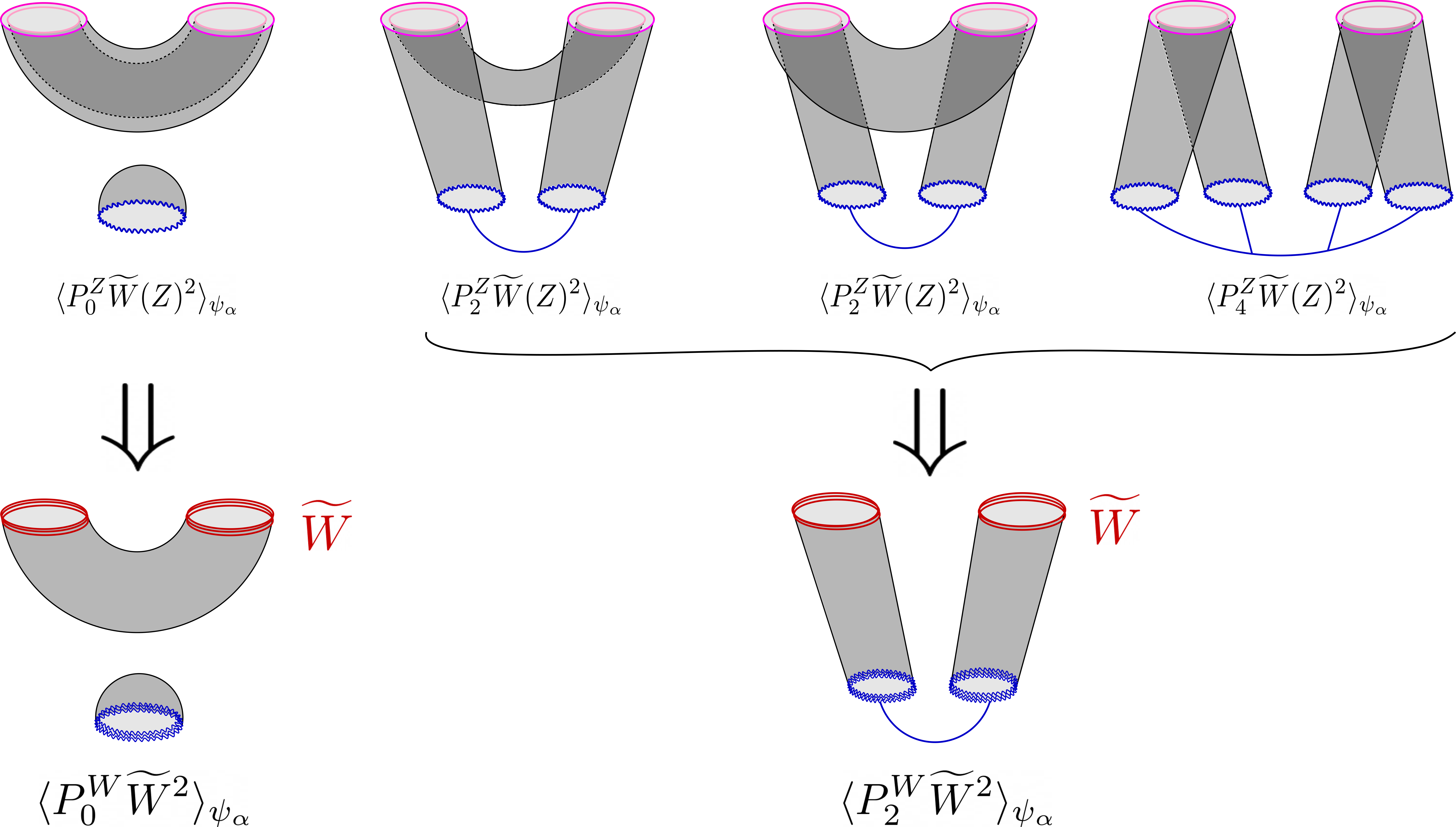
We can then reorganize the above terms in to the following groups
| (368) |
which effectively defines the projector
| (369) | ||||
| (370) |
This rewriting is depicted in Figure 9. To reiterate our logic, we have treated as a new boundary operator, denoted by multiple-wound red circles. The so defined projects into the “-universe” states with boundaries. Note that is not Gaussian, so in principle we can draw the last diagram in the second line of Figure 9 as a pair of pants with two boundaries and one boundary. But we keep the linked boundary figure to remind the reader that later this contribution is identified with the contribution from the half wormholes.
From the first line of Figure 9, we read out the expressions for the different terms in . In particular, we find
| (371) | ||||
| (372) |
Recall that the left hand side of-(372) is just so we obtain
| (373) |
The second term of (365) is off-diagonal and only contribute to and thus
| (374) |
Combing (373) and (374) we get
| (375) | |||
| (376) |
which exactly reproduces the half-wormhole saddle computed directly in the SYK model Mukhametzhanov:2021nea . Notice that for this case with , automatically means . For larger values of this property is no longer true, but this is compensated by the fact that more diagrams contribute to and one can check that the result still matches with the result from the SYK model Mukhametzhanov:2021nea . In addition, the wormhole/half-wormhole saddle decomposition in the SYK computation when and exactly matches with our CGS computation via the mapping (359) we setup in this section, namely
| (377) |
We can further introduce global symmetries such as flavors to the SYK model such as in Gross:2016kjj , then we would get
| (378) |
which is an analogue of (346). Similarly, we can interpret the second term as the half-wormhole.
6.5 A vanishing limit of the CGS model
The CGS model is defined on surfaces. However, due to the relatively simple topologies allowed in the model, it is straightforward to define a 1D theory that consists of lines with no intersection or bifurcation. They can be thought of as the limit of the CGS model where all the circular boundaries, and possibly the disks attached ending on them, shrink to points and the cylinders shrink to lines. We can thus also consider this model as a “vanishing” limit of the CGS model.
We find all results of the CGS model carry through in this limit. Even in cases where the boundary circles are identified with some thermal cycles, we can still consider their infinite temperature limit and deduce the results for the 1D model.
Notice that this limit is not well-defined in the more general surface theory defined in Marolf:2020xie ; the genera on those surfaces will all shrink to loops in this 1D theory, but the shrinking results are not unique even for the simplest genus 1 case. Therefore only for the CGS, namely the surfaces are all disks or cylinders so that there are no nontrivial cycles on the surface that are not homologous to the boundary of the surface, this shrinking process is well defined. That is why we consider this limit only for this CGS model.
It turns out that we can use this 1D theory as the lines and by introducing large numbers of the lines and knitting them together (so that the lines do not bifurcate and this theory remains free), leads to a discrete version of the 2D theory.
This provides an alternative, but speculative, interpretation of the computation in the previous section; the boundary could be considered as creating a 1D boundary that is a wormhole with vanishing size while the creates the usual boundary.
6.6 CGS model with matters
As we have shown in the previous sections, if we couple the surface theory with matters, will in general be described by a compound Poisson distribution. We can consider a similar Disk-Cylinder approximation of in the sense that only the disk and cylinder topologies are taken into account. In this model, there is an analogue of (345) with matter contribution turned on. Let us consider a general boundary operator , the generating function in the Disk-Cylinder limit becomes
| (379) |
So effectively we end up with a family of Gaussian random variables and we can introduce the -universe states following Saad:2021uzi . We denote the one-universe state with fixed value of as and the states of -universes with fixed values as . Here we have chosen the continuous basis for the matter field because it is easier to show the computation. Then all the form a complete basis for the 1-universe state. We can define a projector
| (380) |
Let be some -state and adopting the same trick of introducing as in Saad:2021uzi , we compute the 1-point function
| (381) |
and the two-point function
| (382) |
Using the relation
| (383) |
and equalizing we find
| (384) | |||
| (385) |
which is a simple generalization of (345). One way to fix the inner product is to use the relation (383). First we need to compute , the gravity contribution gives Cyl since it has a cylinder topology. The matter contribution should be
| (386) |
Therefore (383) implies
| (387) |
Acknowledgements.
We thank many members of KITS for interesting discussions. CP is supported by the Fundamental Research Funds for the Central Universities, funds from the University of Chinese Academy of Science (UCAS), and funds from the Kavli Institute for Theoretical Science (KITS). JT is supported by the UCAS program of special research associate and by the internal funds of KITS.Appendix A A summation of winding modes
First consider the simplest case with one boundary, on which one particle is created and then absorbed. Again we only focus on the single connected contribution. his correspond to
| (388) |
where the represents the 1 topologically distinct way of the particle to travel in the bulk. Notice that the order of the boundary insertion is fixed by the orientation of the bulk surface relative to the boundary. Notice that in the presence of matter fields, the definition of the partition function now becomes
| (389) |
where is the Euler characteristic of the surface connected to the boundary and is the chemical potential conjugate to the winding number around non-contractible cycles on the surface. In the following, we first consider the simple example where there is only one flavor of boundaries and one flavor of matter field.
An illustration of this is shown in Fig. 10
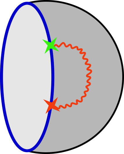
Then we consider the two boundary case
| (390) | |||
| (391) | |||
| (392) | |||
| (393) |
where represents winding times clock-wisely on the cylinder and represents winding times counter-clockwise. In principle we can take to relate the two directions, but if this is imposed the sum does not converge. Therefore as a regulator we do not take , or equivalently we take , so that the above sum converges. At the very end we can choose to set .
An illustration of this computation is shown in Fig. 11. Further notice that in the current counting we allow the trajectories of the different particles to intersect.
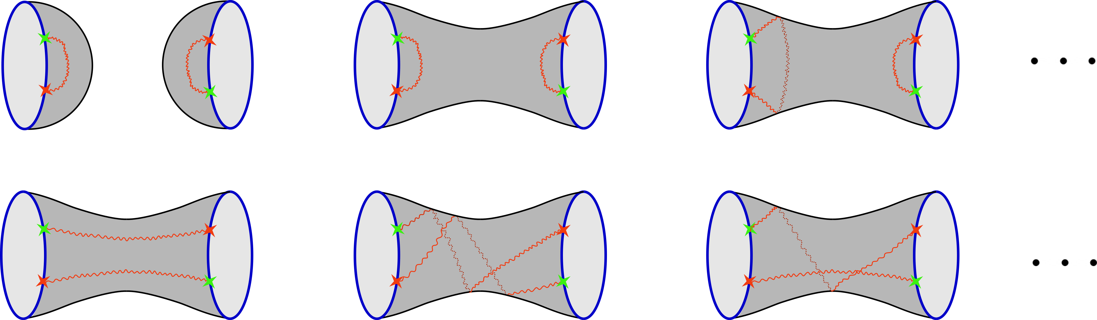
Now we see another version of the factorization puzzle
| (394) |
This is a refined version of the factorization problem, which is the simplified version of the non-vanishing of in the more general (higher dimensional) field theory consideration. Resolving this puzzle gives information about the matter excitations that contribute to the state or the wavefunction.
Appendix B Some simple checks of the truncation proposals
The idea is to rewrite the CCP, which is usually defined as
| (395) |
into the new basis
| (396) |
To illustrate how the procedure discussed in section (3.2), let us consider some simple examples. For the free scalar example, the CCP is given by
| (397) |
Suppose we want to compute the moments up to , whose expressions are known to us
| (398) |
To verify how the procedure work, we truncate the series to and solve for
| (399) | |||
| (400) |
The the general expression of the infinite summations (401)
| (401) |
truncates and can be carried out explicitly. We can perform this sum with two steps: first we fix and sum over all the then take the average of in the Poisson distribution. Fixing , the (401) reduces to
| (402) |
where we have defined convenient parameters . Therefore we can think of are random variables of Poisson distributions with parameters . Then it is easy to obtain first few powers of
| (403) |
which after substituting into (400) equals to
| (404) |
Indeed taking the average of in the Poisson distribution leads to (398). And (402) gives the wrong result of the coefficient at the next order
| (405) |
as expected.
Next, let us consider one flavor of free real matter theory with doubleton insertion, the CCP is then given by
| (406) |
We again truncate the series up to then we can solve
| (407) | |||
| (408) |
The first three moments are still given by the coefficients of in (403) but with new . Substituting (407) into (403) leads to
| (409) |
and
| (410) | |||
| (411) |
which also match our previous results.
As the last example, let us consider the mixture of singleton and doubleton insertions discussed in section 4.3. The corresponding CCP can be obtained by expanding the logarithm of the SCP (130). Then the change of basis leads to
| (412) |
where we have truncated the series up to . The solution is
| (413) | |||
| (414) | |||
| (415) |
Then one can compute the following correlation functions before taking the average
| (416) | |||
| (417) |
References
- (1) G. Penington, “Entanglement Wedge Reconstruction and the Information Paradox,” JHEP 09, 002 (2020) doi:10.1007/JHEP09(2020)002 [arXiv:1905.08255 [hep-th]].
- (2) A. Almheiri, N. Engelhardt, D. Marolf and H. Maxfield, “The entropy of bulk quantum fields and the entanglement wedge of an evaporating black hole,” JHEP 12, 063 (2019) doi:10.1007/JHEP12(2019)063 [arXiv:1905.08762 [hep-th]].
- (3) A. Almheiri, R. Mahajan, J. Maldacena and Y. Zhao, “The Page curve of Hawking radiation from semiclassical geometry,” JHEP 03, 149 (2020) doi:10.1007/JHEP03(2020)149 [arXiv:1908.10996 [hep-th]].
- (4) G. Penington, S. H. Shenker, D. Stanford and Z. Yang, “Replica wormholes and the black hole interior,” [arXiv:1911.11977 [hep-th]].
- (5) A. Almheiri, T. Hartman, J. Maldacena, E. Shaghoulian and A. Tajdini, “Replica Wormholes and the Entropy of Hawking Radiation,” JHEP 05, 013 (2020) doi:10.1007/JHEP05(2020)013 [arXiv:1911.12333 [hep-th]].
- (6) D. N. Page, “Information in black hole radiation,” Phys. Rev. Lett. 71, 3743-3746 (1993) doi:10.1103/PhysRevLett.71.3743 [arXiv:hep-th/9306083 [hep-th]].
- (7) D. N. Page, “Time Dependence of Hawking Radiation Entropy,” JCAP 09, 028 (2013) doi:10.1088/1475-7516/2013/09/028 [arXiv:1301.4995 [hep-th]].
- (8) S. W. Hawking, “Breakdown of Predictability in Gravitational Collapse,” Phys. Rev. D 14, 2460-2473 (1976) doi:10.1103/PhysRevD.14.2460
- (9) P. Saad, S. H. Shenker and D. Stanford, “A semiclassical ramp in SYK and in gravity,” [arXiv:1806.06840 [hep-th]].
- (10) E. Witten, “A Note On Complex Spacetime Metrics,” [arXiv:2111.06514 [hep-th]].
- (11) J. Cotler and K. Jensen, “Gravitational Constrained Instantons,” Phys. Rev. D 104, 081501 (2021) doi:10.1103/PhysRevD.104.L081501 [arXiv:2010.02241 [hep-th]].
- (12) D. Stanford and E. Witten, “JT gravity and the ensembles of random matrix theory,” Adv. Theor. Math. Phys. 24, no.6, 1475-1680 (2020) doi:10.4310/ATMP.2020.v24.n6.a4 [arXiv:1907.03363 [hep-th]].
- (13) P. Saad, S. H. Shenker, D. Stanford and S. Yao, “Wormholes without averaging,” [arXiv:2103.16754 [hep-th]].
- (14) A. Hebecker, T. Mikhail and P. Soler, “Euclidean wormholes, baby universes, and their impact on particle physics and cosmology,” Front. Astron. Space Sci. 5, 35 (2018) doi:10.3389/fspas.2018.00035 [arXiv:1807.00824 [hep-th]].
- (15) A. Kundu, “Wormholes & Holography: An Introduction,” [arXiv:2110.14958 [hep-th]].
- (16) S. W. Hawking, “Quantum Coherence Down the Wormhole,” Phys. Lett. B 195, 337 (1987) doi:10.1016/0370-2693(87)90028-1
- (17) S. B. Giddings and A. Strominger, “Axion Induced Topology Change in Quantum Gravity and String Theory,” Nucl. Phys. B 306, 890-907 (1988) doi:10.1016/0550-3213(88)90446-4
- (18) G. V. Lavrelashvili, V. A. Rubakov and P. G. Tinyakov, “Disruption of Quantum Coherence upon a Change in Spatial Topology in Quantum Gravity,” JETP Lett. 46, 167-169 (1987)
- (19) S. W. Hawking, “Wormholes in Space-Time,” Phys. Rev. D 37, 904-910 (1988) doi:10.1103/PhysRevD.37.904
- (20) S. R. Coleman, “Black Holes as Red Herrings: Topological Fluctuations and the Loss of Quantum Coherence,” Nucl. Phys. B 307, 867-882 (1988) doi:10.1016/0550-3213(88)90110-1
- (21) S. B. Giddings and A. Strominger, “Baby Universes, Third Quantization and the Cosmological Constant,” Nucl. Phys. B 321, 481-508 (1989) doi:10.1016/0550-3213(89)90353-2
- (22) S. B. Giddings and A. Strominger, “Loss of Incoherence and Determination of Coupling Constants in Quantum Gravity,” Nucl. Phys. B 307, 854-866 (1988) doi:10.1016/0550-3213(88)90109-5
- (23) J. Polchinski and A. Strominger, “A Possible resolution of the black hole information puzzle,” Phys. Rev. D 50, 7403-7409 (1994) doi:10.1103/PhysRevD.50.7403 [arXiv:hep-th/9407008 [hep-th]].
- (24) J. McNamara and C. Vafa, [arXiv:2004.06738 [hep-th]].
- (25) T. D. Brennan, F. Carta and C. Vafa, “The String Landscape, the Swampland, and the Missing Corner,” PoS TASI2017, 015 (2017) doi:10.22323/1.305.0015 [arXiv:1711.00864 [hep-th]].
- (26) E. Palti, “The Swampland: Introduction and Review,” Fortsch. Phys. 67, no.6, 1900037 (2019) doi:10.1002/prop.201900037 [arXiv:1903.06239 [hep-th]].
- (27) E. Witten and S. T. Yau, “Connectedness of the boundary in the AdS / CFT correspondence,” Adv. Theor. Math. Phys. 3, 1635-1655 (1999) doi:10.4310/ATMP.1999.v3.n6.a1 [arXiv:hep-th/9910245 [hep-th]].
- (28) J. M. Maldacena and L. Maoz, “Wormholes in AdS,” JHEP 02, 053 (2004) doi:10.1088/1126-6708/2004/02/053 [arXiv:hep-th/0401024 [hep-th]].
- (29) R. Jackiw, “Lower Dimensional Gravity,” Nucl. Phys. B 252, 343-356 (1985) doi:10.1016/0550-3213(85)90448-1
- (30) C. Teitelboim, “Gravitation and Hamiltonian Structure in Two Space-Time Dimensions,” Phys. Lett. B 126, 41-45 (1983) doi:10.1016/0370-2693(83)90012-6
- (31) J. Maldacena and D. Stanford, “Remarks on the Sachdev-Ye-Kitaev model,” Phys. Rev. D 94, no.10, 106002 (2016) doi:10.1103/PhysRevD.94.106002 [arXiv:1604.07818 [hep-th]].
- (32) A. Kitaev and S. J. Suh, “The soft mode in the Sachdev-Ye-Kitaev model and its gravity dual,” JHEP 05, 183 (2018) doi:10.1007/JHEP05(2018)183 [arXiv:1711.08467 [hep-th]].
- (33) S. Sachdev and J. Ye, “Gapless spin fluid ground state in a random, quantum Heisenberg magnet,” Phys. Rev. Lett. 70, 3339 (1993) doi:10.1103/PhysRevLett.70.3339 [arXiv:cond-mat/9212030 [cond-mat]].
-
(34)
A. Kitaev, ”A simple model of quantum holography.” Talks at KITP
http://online.kitp.ucsb.edu/online/entangled15/kitaev/ and
http://online.kitp.ucsb.edu/online/entangled15/kitaev2
A. Kitaev, ”Hidden correlations in the Hawking radiation and thermal noise.” Talk at KITP http://online.kitp.ucsb.edu/online/joint98/kitaev/ - (35) P. Saad, S. H. Shenker and D. Stanford, “JT gravity as a matrix integral,” [arXiv:1903.11115 [hep-th]].
- (36) L. V. Iliesiu, “On 2D gauge theories in Jackiw-Teitelboim gravity,” [arXiv:1909.05253 [hep-th]].
- (37) D. Kapec, R. Mahajan and D. Stanford, “Matrix ensembles with global symmetries and ’t Hooft anomalies from 2d gauge theory,” JHEP 04, 186 (2020) doi:10.1007/JHEP04(2020)186 [arXiv:1912.12285 [hep-th]].
- (38) H. Maxfield and G. J. Turiaci, “The path integral of 3D gravity near extremality; or, JT gravity with defects as a matrix integral,” JHEP 01, 118 (2021) doi:10.1007/JHEP01(2021)118 [arXiv:2006.11317 [hep-th]].
- (39) E. Witten, “Matrix Models and Deformations of JT Gravity,” Proc. Roy. Soc. Lond. A 476, no.2244, 20200582 (2020) doi:10.1098/rspa.2020.0582 [arXiv:2006.13414 [hep-th]].
- (40) I. Aref’eva and I. Volovich, “Gas of Baby Universes in JT Gravity and Matrix Models,” Symmetry 12, no.6, 975 (2020) doi:10.3390/sym12060975 [arXiv:1905.08207 [hep-th]].
- (41) P. Betzios and O. Papadoulaki, “Liouville theory and Matrix models: A Wheeler DeWitt perspective,” JHEP 09, 125 (2020) doi:10.1007/JHEP09(2020)125 [arXiv:2004.00002 [hep-th]].
- (42) D. Anninos and B. Mühlmann, “Notes on matrix models (matrix musings),” J. Stat. Mech. 2008, 083109 (2020) doi:10.1088/1742-5468/aba499 [arXiv:2004.01171 [hep-th]].
- (43) M. Berkooz, V. Narovlansky and H. Raj, “Complex Sachdev-Ye-Kitaev model in the double scaling limit,” JHEP 02, 113 (2021) doi:10.1007/JHEP02(2021)113 [arXiv:2006.13983 [hep-th]].
- (44) T. G. Mertens and G. J. Turiaci, “Liouville quantum gravity – holography, JT and matrices,” JHEP 01, 073 (2021) doi:10.1007/JHEP01(2021)073 [arXiv:2006.07072 [hep-th]].
- (45) G. J. Turiaci, M. Usatyuk and W. W. Weng, “Dilaton-gravity, deformations of the minimal string, and matrix models,” doi:10.1088/1361-6382/ac25df [arXiv:2011.06038 [hep-th]].
- (46) D. Anninos and B. Mühlmann, “Matrix integrals & finite holography,” JHEP 06, 120 (2021) doi:10.1007/JHEP06(2021)120 [arXiv:2012.05224 [hep-th]].
- (47) P. Gao, D. L. Jafferis and D. K. Kolchmeyer, “An effective matrix model for dynamical end of the world branes in Jackiw-Teitelboim gravity,” [arXiv:2104.01184 [hep-th]].
- (48) V. Godet and C. Marteau, “From black holes to baby universes in CGHS gravity,” JHEP 07, 138 (2021) doi:10.1007/JHEP07(2021)138 [arXiv:2103.13422 [hep-th]].
- (49) C. V. Johnson, F. Rosso and A. Svesko, “Jackiw-Teitelboim supergravity as a double-cut matrix model,” Phys. Rev. D 104, no.8, 086019 (2021) doi:10.1103/PhysRevD.104.086019 [arXiv:2102.02227 [hep-th]].
- (50) A. Blommaert and M. Usatyuk, “Microstructure in matrix elements,” [arXiv:2108.02210 [hep-th]].
- (51) K. Okuyama and K. Sakai, “JT gravity, KdV equations and macroscopic loop operators,” JHEP 01, 156 (2020) doi:10.1007/JHEP01(2020)156 [arXiv:1911.01659 [hep-th]].
- (52) S. Forste, H. Jockers, J. Kames-King and A. Kanargias, “Deformations of JT Gravity via Topological Gravity and Applications,” [arXiv:2107.02773 [hep-th]].
- (53) A. Maloney and E. Witten, “Averaging over Narain moduli space,” JHEP 10, 187 (2020) doi:10.1007/JHEP10(2020)187 [arXiv:2006.04855 [hep-th]].
- (54) N. Afkhami-Jeddi, H. Cohn, T. Hartman and A. Tajdini, “Free partition functions and an averaged holographic duality,” JHEP 01, 130 (2021) doi:10.1007/JHEP01(2021)130 [arXiv:2006.04839 [hep-th]].
- (55) J. Cotler and K. Jensen, “AdS3 gravity and random CFT,” JHEP 04, 033 (2021) doi:10.1007/JHEP04(2021)033 [arXiv:2006.08648 [hep-th]].
- (56) A. Pérez and R. Troncoso, “Gravitational dual of averaged free CFT’s over the Narain lattice,” JHEP 11, 015 (2020) doi:10.1007/JHEP11(2020)015 [arXiv:2006.08216 [hep-th]].
- (57) J. Cotler and K. Jensen, “AdS3 wormholes from a modular bootstrap,” JHEP 11, 058 (2020) doi:10.1007/JHEP11(2020)058 [arXiv:2007.15653 [hep-th]].
- (58) M. Ashwinkumar, M. Dodelson, A. Kidambi, J. M. Leedom and M. Yamazaki, “Chern-Simons Invariants from Ensemble Averages,” doi:10.1007/JHEP08(2021)044 [arXiv:2104.14710 [hep-th]].
- (59) N. Afkhami-Jeddi, A. Ashmore and C. Cordova, “Calabi-Yau CFTs and Random Matrices,” [arXiv:2107.11461 [hep-th]].
- (60) S. Collier and A. Maloney, “Wormholes and Spectral Statistics in the Narain Ensemble,” [arXiv:2106.12760 [hep-th]].
- (61) N. Benjamin, S. Collier, A. L. Fitzpatrick, A. Maloney and E. Perlmutter, “Harmonic analysis of 2d CFT partition functions,” doi:10.1007/JHEP09(2021)174 [arXiv:2107.10744 [hep-th]].
- (62) J. Dong, T. Hartman and Y. Jiang, “Averaging over moduli in deformed WZW models,” doi:10.1007/JHEP09(2021)185 [arXiv:2105.12594 [hep-th]].
- (63) A. Dymarsky and A. Shapere, “Comments on the holographic description of Narain theories,” JHEP 10, 197 (2021) doi:10.1007/JHEP10(2021)197 [arXiv:2012.15830 [hep-th]].
- (64) V. Meruliya, S. Mukhi and P. Singh, “Poincaré Series, 3d Gravity and Averages of Rational CFT,” JHEP 04, 267 (2021) doi:10.1007/JHEP04(2021)267 [arXiv:2102.03136 [hep-th]].
- (65) P. Saad, “Late Time Correlation Functions, Baby Universes, and ETH in JT Gravity,” [arXiv:1910.10311 [hep-th]].
- (66) A. Blommaert, T. G. Mertens and H. Verschelde, “Eigenbranes in Jackiw-Teitelboim gravity,” JHEP 02, 168 (2021) doi:10.1007/JHEP02(2021)168 [arXiv:1911.11603 [hep-th]].
- (67) S. B. Giddings and G. J. Turiaci, “Wormhole calculus, replicas, and entropies,” JHEP 09, 194 (2020) doi:10.1007/JHEP09(2020)194 [arXiv:2004.02900 [hep-th]].
- (68) N. Benjamin, S. Collier and A. Maloney, “Pure Gravity and Conical Defects,” JHEP 09, 034 (2020) doi:10.1007/JHEP09(2020)034 [arXiv:2004.14428 [hep-th]].
- (69) A. Blommaert, “Dissecting the ensemble in JT gravity,” [arXiv:2006.13971 [hep-th]].
- (70) E. Gesteau and M. J. Kang, “Holographic baby universes: an observable story,” [arXiv:2006.14620 [hep-th]].
- (71) R. Bousso and E. Wildenhain, “Gravity/ensemble duality,” Phys. Rev. D 102, no.6, 066005 (2020) doi:10.1103/PhysRevD.102.066005 [arXiv:2006.16289 [hep-th]].
- (72) D. Stanford, “More quantum noise from wormholes,” [arXiv:2008.08570 [hep-th]].
- (73) D. Harlow and E. Shaghoulian, “Global symmetry, Euclidean gravity, and the black hole information problem,” JHEP 04, 175 (2021) doi:10.1007/JHEP04(2021)175 [arXiv:2010.10539 [hep-th]].
- (74) C. Peng, “Ensemble averages, Poisson processes, and microstates,” Phys. Rev. D 103, no.6, L061901 (2021) doi:10.1103/PhysRevD.103.L061901 [arXiv:2010.11192 [hep-th]].
- (75) A. M. García-García and V. Godet, “Euclidean wormhole in the Sachdev-Ye-Kitaev model,” Phys. Rev. D 103, no.4, 046014 (2021) doi:10.1103/PhysRevD.103.046014 [arXiv:2010.11633 [hep-th]].
- (76) A. Goel, L. V. Iliesiu, J. Kruthoff and Z. Yang, “Classifying boundary conditions in JT gravity: from energy-branes to -branes,” JHEP 04, 069 (2021) doi:10.1007/JHEP04(2021)069 [arXiv:2010.12592 [hep-th]].
- (77) Y. Chen and H. W. Lin, “Signatures of global symmetry violation in relative entropies and replica wormholes,” JHEP 03, 040 (2021) doi:10.1007/JHEP03(2021)040 [arXiv:2011.06005 [hep-th]].
- (78) P. S. Hsin, L. V. Iliesiu and Z. Yang, “A violation of global symmetries from replica wormholes and the fate of black hole remnants,” Class. Quant. Grav. 38, no.19, 194004 (2021) doi:10.1088/1361-6382/ac2134 [arXiv:2011.09444 [hep-th]].
- (79) T. Anegawa, N. Iizuka, K. Tamaoka and T. Ugajin, “Wormholes and holographic decoherence,” JHEP 03, 214 (2021) doi:10.1007/JHEP03(2021)214 [arXiv:2012.03514 [hep-th]].
- (80) A. Belin, J. De Boer, P. Nayak and J. Sonner, “Charged Eigenstate Thermalization, Euclidean Wormholes and Global Symmetries in Quantum Gravity,” [arXiv:2012.07875 [hep-th]].
- (81) D. Marolf and J. E. Santos, “AdS Euclidean wormholes,” Class. Quant. Grav. 38, no.22, 224002 (2021) doi:10.1088/1361-6382/ac2cb7 [arXiv:2101.08875 [hep-th]].
- (82) O. Janssen, M. Mirbabayi and P. Zograf, “Gravity as an ensemble and the moment problem,” JHEP 06, 184 (2021) doi:10.1007/JHEP06(2021)184 [arXiv:2103.12078 [hep-th]].
- (83) J. Cotler and K. Jensen, “Wormholes and black hole microstates in AdS/CFT,” JHEP 09, 001 (2021) doi:10.1007/JHEP09(2021)001 [arXiv:2104.00601 [hep-th]].
- (84) H. Verlinde, “Wormholes in Quantum Mechanics,” [arXiv:2105.02129 [hep-th]].
- (85) H. Verlinde, “Deconstructing the Wormhole: Factorization, Entanglement and Decoherence,” [arXiv:2105.02142 [hep-th]].
- (86) A. Altland, D. Bagrets, P. Nayak, J. Sonner and M. Vielma, “From operator statistics to wormholes,” Phys. Rev. Res. 3, no.3, 033259 (2021) doi:10.1103/PhysRevResearch.3.033259 [arXiv:2105.12129 [hep-th]].
- (87) B. Freivogel, D. Nikolakopoulou and A. F. Rotundo, “Wormholes from Averaging over States,” [arXiv:2105.12771 [hep-th]].
- (88) A. Blommaert and J. Kruthoff, “Gravity without averaging,” [arXiv:2107.02178 [hep-th]].
- (89) D. Stanford, Z. Yang and S. Yao, “Subleading Weingartens,” [arXiv:2107.10252 [hep-th]].
- (90) J. Raeymaekers, “A note on ensemble holography for rational tori,” [arXiv:2110.08833 [hep-th]].
- (91) P. Betzios, E. Kiritsis and O. Papadoulaki, “Interacting systems and wormholes,” [arXiv:2110.14655 [hep-th]].
- (92) X. L. Qi, Z. Shangnan and Z. Yang, “Holevo Information and Ensemble Theory of Gravity,” [arXiv:2111.05355 [hep-th]].
- (93) A. Almheiri and H. W. Lin, “The Entanglement Wedge of Unknown Couplings,” [arXiv:2111.06298 [hep-th]].
- (94) J. J. Heckman, A. P. Turner and X. Yu, “Disorder Averaging and its UV (Dis)Contents,” [arXiv:2111.06404 [hep-th]].
- (95) A. Blommaert, L. V. Iliesiu and J. Kruthoff, “Gravity factorized,” [arXiv:2111.07863 [hep-th]].
- (96) J. Ambjørn, Y. Sato and Y. Watabiki, “Wormholes, a fluctuating cosmological constant and the Coleman mechanism,” Phys. Lett. B 815, 136152 (2021) doi:10.1016/j.physletb.2021.136152 [arXiv:2101.00478 [hep-th]].
- (97) X. Dong, S. McBride and W. W. Weng, “Replica Wormholes and Holographic Entanglement Negativity,” [arXiv:2110.11947 [hep-th]].
- (98) N. Engelhardt, S. Fischetti and A. Maloney, “Free energy from replica wormholes,” Phys. Rev. D 103, no.4, 046021 (2021) doi:10.1103/PhysRevD.103.046021 [arXiv:2007.07444 [hep-th]].
- (99) E. Casali, D. Marolf, H. Maxfield and M. Rangamani, “Baby Universes and Worldline Field Theories,” [arXiv:2101.12221 [hep-th]].
- (100) L. V. Iliesiu, M. Kologlu and G. J. Turiaci, “Supersymmetric indices factorize,” [arXiv:2107.09062 [hep-th]].
- (101) D. Marolf and H. Maxfield, “Transcending the ensemble: baby universes, spacetime wormholes, and the order and disorder of black hole information,” JHEP 08, 044 (2020) doi:10.1007/JHEP08(2020)044 [arXiv:2002.08950 [hep-th]].
- (102) P. Saad, S. Shenker and S. Yao, “Comments on wormholes and factorization,” [arXiv:2107.13130 [hep-th]].
- (103) B. Mukhametzhanov, “Half-wormholes in SYK with one time point,” [arXiv:2105.08207 [hep-th]].
- (104) A. M. García-García and V. Godet, “Half-wormholes in nearly AdS2 holography,” [arXiv:2107.07720 [hep-th]].
- (105) S. Choudhury and K. Shirish, “Wormhole calculus without averaging from tensor model,” [arXiv:2106.14886 [hep-th]].
- (106) B. Mukhametzhanov, “Factorization and complex couplings in SYK and in Matrix Models,” [arXiv:2110.06221 [hep-th]].
- (107) V. Balasubramanian, A. Kar, S. F. Ross and T. Ugajin, “Spin structures and baby universes,” JHEP 09, 192 (2020) doi:10.1007/JHEP09(2020)192 [arXiv:2007.04333 [hep-th]].
- (108) J. G. Gardiner and S. Megas, “2d TQFTs and baby universes,” JHEP 10, 052 (2021) doi:10.1007/JHEP10(2021)052 [arXiv:2011.06137 [hep-th]].
- (109) N. Arkani-Hamed, T. C. Huang and Y. T. Huang, “The EFT-Hedron,” JHEP 05, 259 (2021) doi:10.1007/JHEP05(2021)259 [arXiv:2012.15849 [hep-th]].
- (110) J. Pollack, M. Rozali, J. Sully and D. Wakeham, “Eigenstate Thermalization and Disorder Averaging in Gravity,” Phys. Rev. Lett. 125, no.2, 021601 (2020) doi:10.1103/PhysRevLett.125.021601 [arXiv:2002.02971 [hep-th]].
- (111) A. Belin and J. de Boer, “Random statistics of OPE coefficients and Euclidean wormholes,” Class. Quant. Grav. 38, no.16, 164001 (2021) doi:10.1088/1361-6382/ac1082 [arXiv:2006.05499 [hep-th]].
- (112) D. J. Gross and V. Rosenhaus, “A Generalization of Sachdev-Ye-Kitaev,” JHEP 02, 093 (2017) doi:10.1007/JHEP02(2017)093 [arXiv:1610.01569 [hep-th]].