The Lick AGN Monitoring Project 2016: Velocity-Resolved H $\beta$ Lags in Luminous Seyfert Galaxies

Vivian U Department of Physics and Astronomy, 4129 Frederick Reines Hall, University of California, Irvine, CA 92697, USA Department of Physics and Astronomy, University of California, Riverside, CA 92521, USA Aaron J. Barth Department of Physics and Astronomy, 4129 Frederick Reines Hall, University of California, Irvine, CA 92697, USA H. Alexander Vogler Department of Physics and Astronomy, 4129 Frederick Reines Hall, University of California, Irvine, CA 92697, USA Department of Physics and Astronomy, University of California, 1 Shields Avenue, Davis, CA 95616, USA Hengxiao Guo Department of Physics and Astronomy, 4129 Frederick Reines Hall, University of California, Irvine, CA 92697, USA Tommaso Treu Department of Physics and Astronomy, University of California, Los Angeles, CA 90095-1547, USA Vardha N. Bennert Physics Department, California Polytechnic State University, San Luis Obispo CA 93407, USA Gabriela Canalizo Department of Physics and Astronomy, University of California, Riverside, CA 92521, USA Alexei V. Filippenko Department of Astronomy, University of California, 501 Campbell Hall, Berkeley, CA 94720-3411, USA Miller Institute for Basic Research in Science, University of California, Berkeley, CA 94720, USA Elinor Gates Lick Observatory, P.O. Box 85, Mt. Hamilton, CA 95140, USA Frederick Hamann Department of Physics and Astronomy, University of California, Riverside, CA 92521, USA Michael D. Joner Department of Physics and Astronomy, N283 ESC, Brigham Young University, Provo, UT 84602, USA Matthew A. Malkan Department of Physics and Astronomy, University of California, Los Angeles, CA 90095-1547, USA Anna Pancoast Harvard-Smithsonian Center for Astrophysics, 60 Garden Street, Cambridge, MA 02138, USA Peter R. Williams Department of Physics and Astronomy, University of California, Los Angeles, CA 90095-1547, USA Jong-Hak Woo Astronomy Program, Department of Physics and Astronomy, Seoul National University, 1 Gwanak-ro, Gwanak-gu, Seoul 08826, Korea SNU Astronomy Research Center, Seoul National University, 1 Gwanak-ro, Gwanak-gu, Seoul 08826, Republic of Korea Bela Abolfathi Department of Physics and Astronomy, 4129 Frederick Reines Hall, University of California, Irvine, CA 92697, USA L. E. Abramson Carnegie Observatories, 813 Santa Barbara Street, Pasadena, CA 91101, USA Stephen F. Armen Department of Astronomy, San Diego State University, San Diego, CA 92182-1221, USA Hyun-Jin Bae Astronomy Program, Department of Physics and Astronomy, Seoul National University, 1 Gwanak-ro, Gwanak-gu, Seoul 08826, Korea Thomas Bohn Department of Physics and Astronomy, University of California, Riverside, CA 92521, USA Benjamin D. Boizelle Department of Physics and Astronomy, N283 ESC, Brigham Young University, Provo, UT 84602, USA Department of Physics and Astronomy, 4129 Frederick Reines Hall, University of California, Irvine, CA 92697, USA Azalee Bostroem Department of Physics and Astronomy, University of California, 1 Shields Avenue, Davis, CA 95616, USA DiRAC Institute, Department of Astronomy, University of Washington, 3910 15th Avenue, NE, Seattle, WA 98195, USA Andrew Brandel Department of Physics and Astronomy, 4129 Frederick Reines Hall, University of California, Irvine, CA 92697, USA Thomas G. Brink Department of Astronomy, University of California, 501 Campbell Hall, Berkeley, CA 94720-3411, USA Sanyum Channa Department of Physics, University of California, Berkeley, CA 94720, USA Department of Physics, Stanford University, Stanford, CA 94305, USA M. C. Cooper Department of Physics and Astronomy, 4129 Frederick Reines Hall, University of California, Irvine, CA 92697, USA Maren Cosens Physics Department, California Polytechnic State University, San Luis Obispo CA 93407, USA Physics Department, University of California, San Diego, 9500 Gilman Drive, La Jolla, CA 92093 USA Center for Astrophysics and Space Sciences, University of California, San Diego, 9500 Gilman Drive, La Jolla, CA 92093 USA Edward Donohue Physics Department, California Polytechnic State University, San Luis Obispo CA 93407, USA Booz Allen, 1615 Murray Canyon Road, Suite 8000, San Diego, CA 92108, USA Sean P. Fillingham Department of Physics and Astronomy, 4129 Frederick Reines Hall, University of California, Irvine, CA 92697, USA Diego González-Buitrago Department of Physics and Astronomy, 4129 Frederick Reines Hall, University of California, Irvine, CA 92697, USA Universidad Nacional Autónoma de México, Instituto de Astronomía, AP 106, Ensenada 22860, BC, México Goni Halevi Department of Astronomy, University of California, 501 Campbell Hall, Berkeley, CA 94720-3411, USA Department of Astrophysical Sciences, Princeton University, 4 Ivy Lane, Princeton, NJ 08544, USA Andrew Halle Department of Physics, University of California, Berkeley, CA 94720, USA Carol E. Hood Department of Physics, California State University, San Bernardino, 5500 University Parkway, San Bernardino, CA 92407, USA Keith Horne SUPA Physics and Astronomy, University of St Andrews, North Haugh, St Andrews, KY16 9SS, Scotland, UK J. Chuck Horst Department of Astronomy, San Diego State University, San Diego, CA 92182-1221, USA Maxime de Kouchkovsky Department of Astronomy, University of California, 501 Campbell Hall, Berkeley, CA 94720-3411, USA Benjamin Kuhn Space Telescope Science Institute, 3700 San Martin Drive, Baltimore, MD 21218, USA Department of Astronomy, San Diego State University, San Diego, CA 92182-1221, USA Sahana Kumar Department of Astronomy, University of California, 501 Campbell Hall, Berkeley, CA 94720-3411, USA Department of Physics, Florida State University, 77 Chieftan Way, Tallahassee, FL 32306, USA Douglas C. Leonard Department of Astronomy, San Diego State University, San Diego, CA 92182-1221, USA Donald Loveland Physics Department, California Polytechnic State University, San Luis Obispo CA 93407, USA Lawrence Livermore National Laboratory, 7000 East Avenue, Livermore, CA 94550 Christina Manzano-King Department of Physics and Astronomy, University of California, Riverside, CA 92521, USA Ian McHardy University of Southampton, Highfield, Southampton, SO17 1BJ, UK Raúl Michel Instituto de Astronomía, Universidad Nacional Autónoma de México, AP 877, Ensenada, Baja California, C.P. 22830 México Melanie Kae B. Olaes Department of Astronomy, San Diego State University, San Diego, CA 92182-1221, USA Daeseong Park Department of Astronomy and Atmospheric Sciences, Kyungpook National University, Daegu, 41566, Republic of Korea Korea Astronomy and Space Science Institute, Daejeon, 34055, Republic of Korea Songyoun Park Astronomy Program, Department of Physics and Astronomy, Seoul National University, 1 Gwanak-ro, Gwanak-gu, Seoul 08826, Korea Liuyi Pei Department of Physics and Astronomy, 4129 Frederick Reines Hall, University of California, Irvine, CA 92697, USA Timothy W. Ross Department of Astronomy, University of California, 501 Campbell Hall, Berkeley, CA 94720-3411, USA Jordan N. Runco Department of Physics and Astronomy, University of California, Los Angeles, CA 90095-1547, USA Jenna Samuel Department of Astronomy, The University of Texas at Austin, 2515 Speedway, Stop C1400, Austin, TX 78712, USA Department of Physics and Astronomy, University of California, 1 Shields Avenue, Davis, CA 95616, USA Javier Sánchez Department of Physics and Astronomy, 4129 Frederick Reines Hall, University of California, Irvine, CA 92697, USA Fermi National Accelerator Laboratory, Kirk Rd. & Pine St, Batavia, IL 60510, USA Kavli Institute for Cosmological Physics, 5640 South Ellis Avenue, Chicago, IL 60637, USA Bryan Scott Department of Physics and Astronomy, University of California, Riverside, CA 92521, USA Remington O. Sexton Department of Physics and Astronomy, University of California, Riverside, CA 92521, USA U.S. Naval Observatory, 3450 Massachusetts Ave NW, Washington, DC 20392-5420, USA Department of Physics and Astronomy, George Mason University, 4400 University Dr, Fairfax, VA 22030-4444, USA Jaejin Shin Astronomy Program, Department of Physics and Astronomy, Seoul National University, 1 Gwanak-ro, Gwanak-gu, Seoul 08826, Korea Isaac Shivvers Department of Astronomy, University of California, 501 Campbell Hall, Berkeley, CA 94720-3411, USA Chance L. Spencer Physics Department, California Polytechnic State University, San Luis Obispo CA 93407, USA Department of Physics, California State University Fresno, Fresno, CA 93740-8031, USA Benjamin E. Stahl Department of Astronomy, University of California, 501 Campbell Hall, Berkeley, CA 94720-3411, USA Department of Physics, University of California, Berkeley, CA 94720, USA Samantha Stegman Department of Astronomy, University of California, 501 Campbell Hall, Berkeley, CA 94720-3411, USA Department of Chemistry, University of Wisconsin, Madison, WI 53706, USA Isak Stomberg Physics Department, California Polytechnic State University, San Luis Obispo CA 93407, USA Deutsches Elektronen-Synchrotron DESY, 22607 Hamburg, Germany Stefano Valenti Department of Physics and Astronomy, University of California, 1 Shields Avenue, Davis, CA 95616, USA L. Villafaña Department of Physics and Astronomy, University of California, Los Angeles, CA 90095-1547, USA Jonelle L. Walsh George P. and Cynthia W. Mitchell Institute for Fundamental Physics and Astronomy, Department of Physics & Astronomy, Texas A&M University, 4242 TAMU, College Station, TX 77843, USA Heechan Yuk Department of Astronomy, University of California, 501 Campbell Hall, Berkeley, CA 94720-3411, USA Department of Physics and Astronomy, University of Oklahoma, 440 W. Brooks St., Norman, OK 73019, USA WeiKang Zheng Department of Astronomy, University of California, 501 Campbell Hall, Berkeley, CA 94720-3411, USA

Abstract

We carried out spectroscopic monitoring of 21 low-redshift Seyfert 1 galaxies using the Kast double spectrograph on the 3 m Shane telescope at Lick Observatory from April 2016 to May 2017. Targeting active galactic nuclei (AGN) with luminosities of $\lambda L_{\lambda}$ (5100 Å) $\approx 10^{44}$ erg s^-1 and predicted H $\beta$ lags of $\sim 20$ –30 days or black hole masses of $10^{7}$ – $10^{8.5}$ M_⊙, our campaign probes luminosity-dependent trends in broad-line region (BLR) structure and dynamics as well as to improve calibrations for single-epoch estimates of quasar black hole masses. Here we present the first results from the campaign, including H $\beta$ emission-line light curves, integrated H $\beta$ lag times (8–30 days) measured against $V$ -band continuum light curves, velocity-resolved reverberation lags, line widths of the broad H $\beta$ components, and virial black hole mass estimates ( $10^{7.1}$ – $10^{8.1}$ M_⊙). Our results add significantly to the number of existing velocity-resolved lag measurements and reveal a diversity of BLR gas kinematics at moderately high AGN luminosities. AGN continuum luminosity appears not to be correlated with the type of kinematics that its BLR gas may exhibit. Follow-up direct modeling of this dataset will elucidate the detailed kinematics and provide robust dynamical black hole masses for several objects in this sample.

Seyfert galaxies, supermassive black holes, active galactic nuclei, reverberation mapping

^†^†software: mpfit (Markwardt, 2009), CARMA (Kelly et al., 2009, 2014), IDL Astronomy User’s Library (Landsman, 1993), IRAF (Tody, 1986), CARAMEL (Pancoast et al., 2011, 2014a, Villafaña et al., in prep.), mapspec (Fausnaugh, 2017)

\turnoffedit

1 Introduction

It has been known for about two decades that black hole (BH) mass exhibits a tight correlation with the stellar velocity dispersion of the galactic bulge within which it resides, and this relation holds over several orders of magnitude in black hole mass (e.g., Ferrarese & Merritt, 2000; Gebhardt et al., 2000). This relation suggests that supermassive black holes and their host galaxies are tightly linked throughout their lifetimes. A fundamental understanding of the growth of supermassive black holes and their interaction with their immediate vicinity will provide key constraints on cosmological models of galaxy evolution Springel et al. (2005); Croton et al. (2006). A crucial component in these numerical recipes is therefore the accurate determination of black hole masses as a function of cosmic history.

Robust black hole mass measurements have been limited mostly to nearby galaxies owing to the exquisite angular resolution needed to spatially resolve a black hole’s sphere of influence. The technique of temporally resolving the structure of the broad-line region (BLR) around an actively accreting black hole, called reverberation mapping (RM; Blandford & McKee, 1982; Peterson, 1993), provides a viable alternative — or in the case of the distant universe, the only currently available — tool for directly measuring black hole masses.

Black hole scaling relations, such as that between the BLR size and the active galactic nuclei (AGN) rest-frame luminosity at 5100 Å (the radius–luminosity relationship; Wandel et al., 1999; Kaspi et al., 2000, 2005; Bentz et al., 2006, 2009a, 2013; Shen, 2013), enable “single-epoch” mass-determination methods for estimating black hole masses in broad-lined AGN out to high redshifts. The calibrations for such mass estimates, however, rest upon the presumptions that distant quasars are similar to the low-redshift reverberation-mapped AGN, while in fact they exhibit higher luminosities and larger Eddington ratios Richards et al. (2011); Shen (2013). Whether virial assumptions for BLR gas dynamics based on local Seyferts can be extended to distant quasars must be tested against a broad range of black hole masses and luminosities. RM, as a tool that probes BLR gas structure, provides the means for such a test.

The RM method is successful for black hole mass determination because the emission lines in the BLR gas are found to respond to the stochastic continuum variations in an AGN via the transfer function Peterson (1993)

L(v_{z},t)=\int^{\infty}_{-\infty}\Psi(v_{z},\tau)~{}C(t-\tau)~{}d\tau\quad,

(1)

where $L(v_{z},t)$ is the emission-line luminosity at line-of-sight velocity $v_{z}$ at observed time $t$ , $C(t)$ is the continuum light curve, and $\Psi(v_{z},\tau)$ is the transfer function that maps continuum variability to the emission-line response at $v_{z}$ after some time delay $\tau$ . This simple model assumes a linear response and no background light; fitting AGN light curves requires the linearized echo model that subtracts off the reference levels, e.g. $L(v_{z},t)-L_{0}(v_{z})$ (see discussion in Horne et al., 2021). Monitoring both the continuum and the emission-line light curves provides data that can allow the determination of $\Psi(v_{z},\tau)$ , also known as the velocity-delay map, whose shape depends on the structure and kinematics of the BLR Horne et al. (2004). In practice, precise velocity-resolved information in the form of the transfer function demands intense monitoring with frequent sampling, high signal-to-noise ratio (S/N) data, and long duration. As a result, the number of AGN with such data available to-date has been limited.

With the goal of refining black hole scaling relations through expanding the local reverberation-mapped AGN database by which they are anchored, we embarked on a campaign aimed to monitor AGN at higher luminosity than samples targeted in the 2008 and 2011 campaigns of the Lick AGN Monitoring Project (LAMP, e.g., Bentz et al., 2009b; Barth et al., 2015). Higher-luminosity AGN tend to have longer lags. Coupled with the fact that they have weaker variability amplitudes owing to the ample fuel supply in their accretion disks vanden Berk et al. (2004); Wilhite et al. (2008); MacLeod et al. (2010), lag recovery is more challenging for these objects. The advent of large, multi-object programs such as SDSS-RM Shen et al. (2015) and OzDES Yuan et al. (2015) provides a new landscape where large numbers of reverberation lags for H $\beta$ , Mg II, and C IV in quasars are determined over a broad redshift range Shen et al. (2016); Grier et al. (2017, 2019). Grier et al. (2017) measured H $\beta$ time lags for 44 AGN with luminosities $\log$ [ $\lambda L_{\lambda}$ (5100 Å)/ $L_{\sun}]\approx 43$ –45.5 at redshifts $z=0.12$ –1. Early results from the SDSS-RM campaign determined C IV lags in 52 quasars Grier et al. (2019), whereas those from OzDES found two C IV-based black hole masses to be among the highest redshift ( $z=1.9$ –2.6) and highest mass black holes [ $M_{\mathrm{BH}}=(3.3$ –4.4) $\times 10^{9}$ M_☉] measured thus far with RM studies Hoormann et al. (2019). Complementing these large multifiber spectroscopic studies, our campaign targeted AGN at low redshifts and aimed to yield high-fidelity data for velocity-resolved lag measurements and dynamical modeling.

During the past several years, different groups have determined resolved velocity-delay reverberation signatures for dozens of unique objects among local Seyferts, changing-look AGN, and those with H $\beta$ asymmetry (e.g., Bentz et al., 2010a; Grier et al., 2013; Pancoast et al., 2014b; De Rosa et al., 2018; Du et al., 2018a; Williams et al., 2018, 2020; Lu et al., 2019; Zhang et al., 2019; Sergeev, 2020; Lu et al., 2021; Bentz et al., 2021). Our primary intent is to use a large, relatively broad sample to investigate statistical luminosity-dependent trends in BLR structure and gas dynamics using velocity-resolved reverberation, which could directly impact the accuracy of virial mass estimates. Here we present our first results that focus on new H $\beta$ velocity-resolved measurements along with integrated H $\beta$ lags and virial black hole masses. Our dataset will allow for forward-modeling work using, for instance, the CARAMEL code (Pancoast et al., 2011, 2014a, Villafaña et al., in prep.) to directly determine black hole masses.

This paper is organized as follows. The sample selection is described in Section 2. In Section 3, we present our observational program at Lick Observatory and details of the data reduction and processing work. Section 4 reports on our photometric campaign to provide the continuum light curves for our AGN sources. In Section 5, we illustrate our emission-line light curves and subsequent integrated and velocity-resolved H $\beta$ lag detections, including an assessment of the lag significance and the observed variety of BLR kinematics. Section 6 depicts our line-width measurements and derived virial black hole masses, within the larger context of how our results compare with the existing AGN radius–luminosity relation.

Throughout the paper, we have adopted $H_{0}=67.8$ km s^-1 Mpc^-1, $\Omega_{\rm m}$ = 0.308, and $\Omega_{\rm vac}$ = 0.692 Planck Collaboration et al. (2016).

2 Sample Selection

The past Lick AGN Monitoring Project (LAMP) campaigns targeted AGN with H $\beta$ lags of $\sim 3$ –15 days (Bentz et al., 2009b, 2010b; Barth et al., 2015). The chief objective of this campaign is to investigate BLR kinematics of moderate-luminosity AGN, so we targeted primarily Seyfert 1s with extinction-corrected $\log$ [ $\lambda L_{\lambda}$ (5100 Å)/ $L_{\sun}$ ] $\approx 43.5$ –43.9. Based on the radius–luminosity relation (e.g., Bentz et al., 2013), the targeted AGN continuum luminosity range corresponds to an H $\beta$ lag range of 20 $-$ 30 days. We note, however, that recent results from the SEAMBH (Du et al., 2016a, 2018b; Du & Wang, 2019) and SDSS-RM (Grier et al., 2017) programs have shown that some AGN have lags shorter than would be expected from earlier versions of the radius–luminosity relation (Bentz et al., 2013).

We applied this 20–30-day criterion in H $\beta$ lag or equivalently $\lambda L_{\lambda}$ (5100 Å) to various catalogs of Type 1 AGN (e.g., Boroson & Green, 1992; Marziani et al., 2003; Peterson et al., 2004; Vestergaard & Peterson, 2006; Bachev et al., 2008; Winter et al., 2010; Shen et al., 2011; Zu et al., 2011; Joshi et al., 2012; Bennert et al., 2015; Sun & Shen, 2015). Our selection was further narrowed with a redshift limit at $z<0.08$ to ensure that the H $\beta$ and [O III] lines fall blueward of the cutoff wavelength of the dichroic used in the Kast spectrograph (5500 Å). Sources were selected with declination $\delta\geq$ $-$ 5° and magnitude $<$ 17 in the optical $V$ or $r$ band. We also assessed the short-term variability in previous light curves from the Catalina Real-time Transient Survey Drake et al. (2009) for all our candidate sources and selected those with at least 0.1 magnitude of variations. Targets having high-quality velocity-resolved lag measurement from previous RM campaigns were excluded (e.g., Denney et al., 2010; Grier et al., 2012; Du et al., 2014; Wang et al., 2014), as were those no longer featuring broad hydrogen recombination lines in archival Lick optical spectra.

In order to ensure that lags can be measured accurately, we placed a further constraint requiring that the monitoring duration of an AGN, defined as the longest continuous period when the AGN can be observed at airmass $<$ 2 during our campaign, be at least 3 times larger than the expected H $\beta$ lag based on simulations. Given that our initial campaign duration was designed to be 9 months long (which extended to 1 year later on), this constraint resulted in a sample of 29 objects with duration-to-lag ratio $>$ 3. Two sources with slightly shorter H $\beta$ lag estimates (Mrk 315: 13 days; Mrk 704: 16 days) were included to better fill the right-ascension range of the sample.

After an initial probationary period of $\sim 1$ month, we discarded 8 sources showing low continuum variability amplitude, retaining a sample of 21 objects for ongoing monitoring. This final sample of Seyfert 1s and their properties are listed in Table 1.

Table 1: Sample Properties

Object	Other Name(s)	Right Ascension	Declination	Redshift	Reference
		(J2000)	(J2000)
Zw 535-012		00:36:20.983	$+$ 45:39:54.08	0.04764	1
I Zw 1	UGC 00545, Mrk 1502, PG 0050+124	00:53:34.940	$+$ 12:41:36.20	0.05890	2
Mrk 1048	NGC 985, VV 285	02:34:37.769	$-$ 08:47:15.44	0.04314	2
Ark 120	UGC 03271, Mrk 1095	05:16:11.421	$-$ 00:08:59.38	0.03271	3
Mrk 376	KUG 0710+457, IRAS 07105+4547	07:14:15.070	$+$ 45:41:55.78	0.05598	3
Mrk 9		07:36:56.979	$+$ 58:46:13.43	0.03987	1,3
Mrk 704	CGCG 091-065, MCG +03-24-043	09:18:26.005	$+$ 16:18:19.22	0.02923	4
MCG +04 $-$ 22 $-$ 042		09:23:43.003	$+$ 22:54:32.64	0.03235	5
Mrk 110	PG 0921+525	09:25:12.870	$+$ 52:17:10.52	0.03529	6,7
RBS 1303	CGS R14.01	13:41:12.904	$-$ 14:38:40.58	0.04179	4
Mrk 684		14:31:04.783	$+$ 28:17:14.11	0.04608	1
Mrk 841	J15040+1026	15:04:01.201	$+$ 10:26:16.15	0.03642	5
Mrk 1392	1505+0342	15:05:56.553	$+$ 03:42:26.32	0.03614	8
SBS 1518+593		15:19:21.650	$+$ 59:08:23.70	0.07810	9
3C 382	CGCG 173-014	18:35:03.390	$+$ 32:41:46.80	0.05787	2
NPM1G+27.0587	2MASX J18530389+2750275	18:53:03.874	$+$ 27:50:27.72	0.06200	10
RXJ 2044.0+2833		20:44:04.500	$+$ 28:33:12.10	0.05000	10
PG 2209+184	II Zw 171	22:11:53.889	$+$ 18:41:49.86	0.07000	2
PG 2214+139	Mrk 304	22:17:12.262	$+$ 14:14:20.89	0.06576	2
RBS 1917	2MASX J22563642+0525167	22:56:36.500	$+$ 05:25:17.20	0.06600	2
Mrk 315		23:04:02.622	$+$ 22:37:27.53	0.03887	1

Note. — Objects in this and subsequent tables and figures are listed in RA order. Redshifts are from NED. References for $\lambda L_{\lambda}$ (5100 Å) used to estimate the H $\beta$ lag in our sample selection: (1) Previous Lick spectra; (2) Marziani et al. (2003); (3) Joshi et al. (2012); (4) Barth et al. (2015); (5) Winter et al. (2010); (6) Peterson et al. (2004); (7) Zu et al. (2011); (8) Bennert et al. (2015); (9) Sun & Shen (2015); (10) Bachev et al. (2008)

3 The Spectroscopic Campaign at Lick

3.1 Overview of the Observational Program

We conducted a spectroscopic monitoring program of 1 yr duration at Lick Observatory on Mount Hamilton, California. Prior to the start of the campaign, we ran simulations to determine the minimum threshold for successful lag recovery among monitoring periods of varying lengths and cadences. Our estimated H $\beta$ lag range required a sampling cadence of two nights per week over the course of a year to sufficiently resolve time-dependent emission-line variations and to extend the temporal baseline for detecting robust reverberation signal across the entire extent of the BLR, accounting for anticipated weather losses and seasonal gaps.

This project was allocated 100 nights at the Lick 3 m Shane telescope across three observing semesters between 2016 April 28 and 2017 May 6 (UT). The observing runs were distributed mostly with a frequency of $\sim 2$ nights per week as requested, with the exception of bright time and occasional scheduling constraints owing to other time-sensitive observing programs. Partial nights were occasionally exchanged with or obtained from other programs to facilitate the sampling cadence of certain targets during this monitoring period.

Spectroscopic data were taken using the Kast Double Spectrograph Miller & Stone (1994). The red CCD detector was upgraded halfway into our campaign (September 17–20, 2016). The upgrade from the Reticon $400\times 1200$ pixel CCD to the Hamamatsu $4096\times 1024$ pixel CCD significantly improved the quantum efficiency, up to a factor of 2 at the red end, and removed severe fringing effects. Images taken with the new red CCD suffered from a high incidence rate of cosmic-ray hits and alpha-particle hits due to radioactive material in the new dewar window. These defects were removed at the reduction stage where frames were combined before the spectrum was extracted.

We employed the following setup for our AGN observations: the D55 dichroic with the 600/4310 grism (nominal coverage of 3300–5520 Å at 1.02 Å/pixel) on the blue side and the 600/7500 grating (nominal coverage of 4000–11,000 Å at 2.35 Å/pixel pre-upgrade, and 3800–10,000 Å at 1.31 Å/pixel post-uprade) on the red side, a compromise between broad spectral coverage and moderate spectral resolution. The plate scale was 0 $\farcs$ 43/pixel for both the blue and the new red detectors, and 0 $\farcs$ 78/pixel for the old red detector. A slit width of 4″ was employed to minimize slit losses due to seeing variations between different nights (Filippenko, 1982). A fixed position angle, optimized for each individual target, was chosen so that the spectroscopic aperture sampled the same portion of the host galaxy across the duration of the monitoring campaign.

Exposure times were typically up to 30 min per object each night, split into 2 or 3 separate exposures (pre- and post-upgrade of the red CCD, respectively) to facilitate cosmic-ray cleaning. Standard calibrations including bias exposures, arc frames (using the Ar, He, Hg, Cd, and Ne lamps), and dome flats were taken during the afternoon, and well-calibrated flux standard stars (G191B2B, Feige 34, BD+284211, HZ44, BD+262606, and/or BD+174708) were observed during the nights. Before the red CCD upgrade, red-side observations suffered from severe fringing at wavelengths longward of 7000 Å. In order to remove the fringe pattern, dome flats at the position of every object were taken before or after each standard star and AGN observation on the red side. This time-consuming procedure was no longer needed after the upgrade that eliminated the fringing effect. The observing parameters for our sample are listed in Table 2.

The wet 2016–2017 winter season at Lick hampered our observing effort, particularly during December through February. Overall, our spectroscopic campaign achieved an observational success rate of $\lesssim 70$ %, where 30 nights were lost entirely to weather or dome issues. For another 12 nights, only 6 or fewer AGN were observed when typically 12–15 objects would have been observed on a night with good conditions. We were confident that at least fourteen nights of observations were carried out under photometric conditions. Of the 70 nights when data were obtained, half were done with the old red CCD and half with the upgraded detector. The number of total epochs observed for each object ranges from 22 to 50, with a median of 38 (see Table 2).

Table 2: Observing Parameters

Object	Slit PA	$t_{\rm exp}$	Monitoring Period	$N_{\rm obs}$	S/N	$N_{\rm phot}$
	(deg)	(s)	(UT)
Zw 535 $-$ 012	100	1800	2016/06/27 $-$ 2017/03/04	41	57	10
I Zw 1	45	1600	2016/07/03 $-$ 2017/02/01	34	103	6
Mrk 1048	0	1800	2016/08/08 $-$ 2017/02/16	27	88	5
Ark 120	0	1800	2016/08/15 $-$ 2017/03/26	34	124	5
Mrk 376	70	1800	2016/05/01 $-$ 2017/05/01	31	84	6
Mrk 9	90	1800	2016/05/01 $-$ 2017/05/01	33	78	5
Mrk 704	130	1800	2016/10/20 $-$ 2017/05/01	23	106	3
MCG +04 $-$ 22 $-$ 042	145	1800	2016/05/01 $-$ 2017/05/01	34	54	7
Mrk 110	44	1200	2016/05/01 $-$ 2017/05/01	41	74	6
RBS 1303	20	1200	2016/05/01 $-$ 2017/05/01	22	67	5
Mrk 684	60	1800	2016/05/01 $-$ 2017/05/01	43	98	12
Mrk 841	50	800	2016/05/01 $-$ 2017/05/01	45	77	11
Mrk 1392	50	1800	2016/05/01 $-$ 2017/05/01	39	55	10
SBS 1518+593	90	1800	2016/05/01 $-$ 2017/05/01	48	44	8
3C 382	70	1800	2016/05/01 $-$ 2016/12/03	50	81	12
NPM1G+27.0587	60	1800	2016/05/01 $-$ 2016/12/03	38	55	7
RXJ 2044.0+2833	60	1800	2016/05/01 $-$ 2016/12/31	46	58	9
PG 2209+184	60	1800	2016/05/01 $-$ 2016/12/31	40	32	9
PG 2214+139	60	1800	2016/05/18 $-$ 2016/12/31	43	81	10
RBS 1917	30	1800	2016/06/01 $-$ 2016/12/31	32	39	9
Mrk 315	60	1800	2016/06/07 $-$ 2016/12/31	35	59	9

Note. — $t_{\rm exp}$ represents the typical total on-source exposure time for each AGN every night it was observed, usually split among 2–4 frames. $N_{\rm obs}$ represents the total number of spectroscopic observations for each source. S/N represents the median S/N per pixel in the continuum at (5100–5200) ( $1+z$ ) Å. $N_{\rm phot}$ represents the number of photometric nights for each source.

3.2 Spectroscopic Data Reduction

The Kast spectroscopic data were reduced using a combination of standard routines in IRAF and IDL, following the procedure outlined by Barth et al. (2015). Here we provide a brief description of the reduction process of the blue-side data and pre-/post-upgrade red-side data.

In general, the data were processed via bias subtraction, flat fielding, cosmic-ray cleaning, one-dimensional (1D) extraction using an unweighted boxcar extraction region, wavelength calibration, and flux calibration. Error spectra were extracted and propagated through all subsequent calibration steps. Multiple spectra taken on the same night were combined. The width adopted for the spectral extraction was 10″, though it was widened to $\sim 15$ –20″ for some sources (Mrk 315, Mrk 9, MCG +04 $-$ 22 $-$ 042, and NPM1G+27.0587) and during particular nights where the seeing was exceptionally poor.

Most of the AGN were flux calibrated using the standard-star exposure that was closest in airmass. However, the flux-calibrated spectra for a few epochs exhibited some abnormal slopes and features close to the dichroic cutoff. We were unable to conclusively determine the cause of these anomalies, but they were most likely related to the dichroic. Since the [O III] $\lambda$ 5007 line, situated close to the dichroic cutoff, was assumed to be constant throughout the observing campaign and was used to normalize the nightly spectra, this peculiarity identified in several spectra added extra scatter to the H $\beta$ light curves. In these cases, we attempted to correct the problem by calibrating the AGN with standard stars that were taken close in time for six nights. As a result, this flux-calibration issue was partially rectified but remained responsible for some residual scatter in the emission-line light curves.

For red-side data taken prior to 2016 Sep. 20, each observation was flattened using a dome-flat exposure taken at the same telescope position. For red-side data taken between 2016 Sep. 20 and 2017 Jan. 31, the Kast red dewar was slightly tilted and thus the two-dimensional spectra had to be adjusted with a rotation of 0.9° before spectral extraction.

3.3 Photometric and Spectral Scaling

To ensure that all the spectra for each AGN are on consistent flux and wavelength scales across the monitoring period, a modified version of the procedure described by van Groningen & Wanders (1992, hereafter VGW92) was applied to the blue-side data for internal calibration (see Barth et al., 2015; Fausnaugh, 2017, for more details). Having the spectra exhibit consistent spectral resolution throughout the temporal series is important particularly for extracting velocity-resolved measurements. First, we computed the shifts in wavelength among the time-series spectra from cross correlation. We applied these shifts to align the spectra and calculated an initial mean spectrum that was then designated as the reference. The [O III] $\lambda$ 5007 fluxes, presumed to be intrinsically constant throughout the course of the observing campaign, were measured from spectra taken during photometric nights and were averaged to estimate the true absolute flux of [O III]. The number of photometric nights designated per object ranged from 3 to 12, with a median of 8 nights. The resulting reference spectrum was then scaled to match this measurement of the [O III] flux, with a median uncertainty of 8%.

Each night’s spectrum was then aligned and scaled to the reference by matching the [O III] $\lambda$ 5007 emission-line profile following our modified VGW92 scaling method. In order to minimize variations outside of intrinsic AGN variability, we aimed to achieve a uniform spectral resolution across the full time series of spectra. Where VGW92 ignores resolution corrections for epochs observed at lower resolution than the reference spectrum, we adopted instead a modified approach similar to that described by Fausnaugh (2017): we first applied a Gaussian broadening kernel to the reference spectrum to ensure that all the rescaled spectra match a single resolution, typically the worst among the spectra. Excluding the occasional extreme outliers, this broadening kernel had a typical $\sigma$ of $\sim 1.5$ –3 Å with a median $\sigma$ of 2 Å for each AGN. Each of the spectra was then aligned by wavelength, scaled in flux, and broadened in spectral resolution to match the [O III] line profile of the broadened reference spectrum.

We performed a comparison of the modified VGW92 spectral scaling method to that using the Python code mapspec Fausnaugh (2017) with the same wavelength windows and broadened reference spectrum. Differences between the two approaches include the following: (i) VGW92 calls for using a Gaussian kernel for smoothing, while mapspec offers an additional option of using Gauss-Hermite polynomials; and (ii) our modified VGW92 approach fits for free parameters via $\chi^{2}$ minimization, while mapspec uses a Bayesian framework to optimize rescaling parameters and estimate model uncertainties. The runtime for the modified VGW92 method was typically $\sim 100$ times shorter than for mapspec. We ran several tests comparing the level of scatter in the light curves of the [O III] line that resulted from both methods and concluded that modified VGW92 performed better for most of the AGN in our sample. We subsequently adopted the spectra scaled with the modified VGW92 approach for the ensuing analysis.

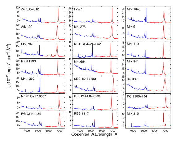
Refer to caption — Figure 1: Mean spectra for the LAMP2016 sample including both blue- and red-side data. Here, as in Table 1, the AGN are shown in order of increasing right ascensions.

The scaling of the red-side data took a different approach. To normalize the red-side flux scale, red-side spectra were stitched to the corresponding blue-side spectra via aligning their overlapping regions ( $\sim 5300$ –5500 Å). All spectra were first aligned to the reference spectrum in wavelength. Because the ends of the spectra tended to be noisy, we used a weighted average to determine the overall multiplicative scaling factor. This technique worked well in most cases where the spectra were smooth or well behaved at the ends. The average scaled spectra for the sample are presented in Figure 1.

3.4 Noise-Corrected RMS Spectra

Relative variability across the spectrum can be visualized using the root-mean-square (rms) spectrum. The Peterson et al. (2004) procedure of taking the standard deviation of flux values at each wavelength element over all the epochs may inadvertently bias the rms spectrum given the inclusion of various noise factors in addition to genuine AGN variability Barth et al. (2015). To remove the contribution due to photon-counting noise from the rms spectrum, Pei et al. (2017) suggested an approach to produce the “excess rms” (e-rms hereafter) spectrum defined per wavelength element $\lambda$ and epoch $i$ as

\textrm{e-rms}_{\lambda}=\sqrt{\frac{1}{N-1}\sum^{N}_{i=1}[(F_{\lambda,i}-\langle F_{\lambda}\rangle)^{2}-\delta^{2}_{\lambda,i}]}\quad,

(2)

where $N$ is the number of epochs in the time series, $\langle F_{\lambda}\rangle$ is the flux averaged over the time series, and $F_{\lambda,i}$ and $\delta_{\lambda,i}$ refer to the flux and rms uncertainty in the flux at each $\lambda$ and $i$ , respectively. This was applied to the set of scaled spectra for each AGN.

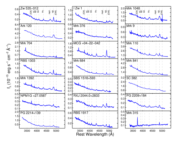
In the case of an AGN with strongly varying broad-line profiles, broad features are expected to dominate the e-rms spectra in the relevant spectral regions. The narrow [O III] lines, on the other hand, generally vanish in the rms given that they are assumed to be constant within the time-series data. Presented in Figure 2, the e-rms spectra generally feature a strong blue continuum (except for Mrk 315), broad-line emission in the Balmer series and (usually) in He II. The absence of residual narrow [O III] features confirms that our internal flux calibration worked well near this wavelength, but other residual narrow-line features are likely artifacts of imperfect flux calibration errors that increase at bluer wavelengths. This is particularly the case for Mrk 315, which has a red e-rms continuum slope and prominent [O II] $\lambda$ 3727.

3.5 Spectral Decomposition

The traditional approach of measuring broad emission-line fluxes using a simple linear continuum subtraction is subject to several inadequacies. A linear continuum model is unable to separate blended emission-line features, such as He II or Fe II lines that often overlap the broad H $\beta$ profile. Furthermore, a linear fit is a poor approximation to the actual continuum, which includes both AGN and host-galaxy components. Residual errors from continuum subtraction can be particularly problematic for velocity-resolved RM in the faint high-velocity wings of broad emission lines, where oversubtraction or undersubtraction of the continuum could lead to biased inferences on BLR structure and kinematics. In recent years, spectral decomposition approaches have been applied to the data from some RM campaigns (e.g., Barth et al., 2013, 2015; Hu et al., 2015). By fitting a multicomponent model to each night’s spectrum, the contributions of individual line and continuum components can be isolated.

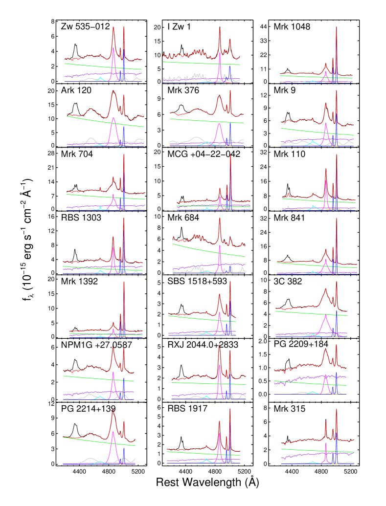
Here we have adopted and applied the spectral fitting method described by Barth et al. (2015) for the H $\beta$ spectral region. We refer the reader to Barth et al. (2015) for a detailed description, and provide a brief overview of the method here. The model components include a power-law AGN continuum, starlight from a single-burst old stellar population at solar metallicity (Bruzual & Charlot, 2003) convolved with a Gaussian velocity broadening, and emission lines including [O III] (narrow), H $\beta$ (broad and narrow), He II (broad and narrow), He I (broad), and an Fe II emission template convolved with a Gaussian velocity broadening. Emission-line profiles were modeled using a fourth-order Gauss-Hermite function, except for the He I and He II lines for which a Gaussian was used. Each line’s velocity centroid was allowed to vary independently, except for the [O III] $\lambda\lambda$ 4959, 5007 lines which were required to have the same velocity profile and a 1:3 flux ratio. For the Fe II blends, we tested different template spectra as described by Boroson & Green (1992), Véron-Cetty et al. (2004), and Kovačević et al. (2010). In the near future, we will employ a promising, new Fe II template spectrum based on Mrk 493 (Park et al., in prep.). Similar to Barth et al. (2015), the multicomponent Kovačević et al. (2010) template provided the best fit to the Fe II lines in all of our AGN and was used for the final fits, except for the case of I Zw 1. For I Zw 1 we found that the Boroson & Green (1992) template, which is based on I Zw 1 itself, provided the best fit with minimized residuals. As part of the fitting process, a Cardelli et al. (1989) reddening model is applied to the model spectrum, allowing $E(B-V)$ to be a free parameter. Fitting was carried out over a rest-wavelength range of approximately 4200–5200 Å, with the exact range tailored to the data for each AGN depending on its redshift. The H $\gamma$ + [O III] $\lambda 4363$ blend was masked out from the fit, because decomposing this blend would add several additional free parameters to the model. The full model, including the multicomponent Kovačević et al. (2010) iron template, includes 33 free parameters. Model fits were optimized using a Levenberg-Marquart algorithm as implemented by Markwardt (2009). For each AGN, the model was first fitted to the mean spectrum, and the fit parameters from the mean spectrum fit were used as the starting parameter estimates for the fit to each individual night’s spectrum. The overall mean spectrum as fitted with the different model components for each galaxy is illustrated in Figure 3.

4 The Photometric Campaign

AGN continuum light curves were measured from imaging data. We chose the $V$ band since it provides a fairly clean continuum measurement with relatively little contamination from broad emission lines for low-redshift sources. To maximize the chances of detecting the delayed response of the emission-line variations to those of the continuum, we began the photometric monitoring campaign two months before the start of the spectroscopic program. From February 2016 to May 2017, our team used a network of eight telescopes across the world and obtained high-fidelity $V$ -band images with up to nightly cadence within each object’s monitoring season.

4.1 Telescopes and Cameras

Our photometric campaign included observations with the following telescopes: the 0.76 m Katzman Automatic Imaging Telescope (KAIT) Filippenko et al. (2001) and the Anna Nickel telescope at Lick Observatory on Mount Hamilton, California; the Las Cumbres Observatories Global Telescope (LCOGT) network Brown et al. (2013); Boroson et al. (2014); the 2 m Liverpool Telescope at the Observatorio del Roque de Los Muchachos on the Canary island of La Palma, Spain Steele et al. (2004); the 1 m Illinois Telescope at Mount Laguna Observatory (MLO; Smith & Nelson, 1969) in the Laguna Mountains, California; the San Pedro Mártir Observatory (SPM) 1.5 m Johnson telescope (Butler et al., 2012; Watson et al., 2012) at the Observatory Astronómico Nacional located in Baja California, México; the Fred Lawrence Whipple Observatory 1.2 m telescope on Mount Hopkins, Arizona; and the 0.9 m West Mountain Observatory (WMO) telescope at Utah Lake in Utah. KAIT, LCOGT, SPM-1.5 m, and Liverpool are fully robotic telescopes. Table 3 summarizes the telescope and detector properties.

Table 3: Telescope and CCD Properties for Imaging Observations

Telescope	$D_{\rm mirror}$	Detector	Field of View	Pixel Scale	Gain	Read Noise	Binning
	(m)			(″/pix)	( $e^{-}$ /ADU)	( $e^{-}$ )
FLWO-1.2 m	1.2	Fairchild CCD 486	23 $\farcm$ 1 $\times$ 23 $\farcm$ 1	0.336	4.45	7.18	2 $\times$ 2
KAIT	0.76	Apogee AP7	6 $\farcm$ 8 $\times$ 6 $\farcm$ 8	0.80	4.5	12.0	1 $\times$ 1
LCOGT-2 m	2.0	Merope	4 $\farcm$ 7 $\times$ 4 $\farcm$ 7	0.467	1.0	9.0	2 $\times$ 2
LCOGT-1 m	1.0	Fairchild Imaging	26 $\farcm$ 5 $\times$ 26 $\farcm$ 5	0.389	1.0	13.5	1 $\times$ 1
Liverpool	2.0	e2V CCD 231	10′ $\times$ 10′	0.304	1.62	8.0	2 $\times$ 2
MLO-1 m	1.0	Fairchild 446	13 $\farcm$ 3 $\times$ 13 $\farcm$ 3	0.718	2.13	3.88	1 $\times$ 1
Nickel	1.0	Loral	6 $\farcm$ 3 $\times$ 6 $\farcm$ 3	0.368	1.7	8.3	2 $\times$ 2
SPM-1.5 m	1.5	Fairchild 3041	5 $\farcm$ 4 $\times$ 5 $\farcm$ 4	0.32	4.2	14.0	2 $\times$ 2
WMO-0.9 m	0.9	Finger Lakes PL-09000	25 $\farcm$ 2 $\times$ 25 $\farcm$ 2	0.61	1.37	12.0	1 $\times$ 1

4.2 Photometry Measurements and Continuum Light Curves

All images were processed with reduction procedures applied as part of the standard pipeline for each facility, including overscan subtraction and flat-fielding. For telescopes that did not include world coordinate system (WCS) solutions as part of their standard processing, we used astrometry.net Lang et al. (2010) to add WCS information to the FITS headers.

Measurement of the AGN light curves was carried out using the automated aperture photometry pipeline described by Pei et al. (2014), which can be used to measure AGN light curves using data from any number of telescopes with diverse camera properties. This procedure, written in IDL and based on the photometry routines in the IDL Astronomy User’s Library (Landsman, 1993), is designed to automate the process of identifying the AGN and a set of comparison stars in each image by their coordinates, measuring their instrumental magnitudes, and using the comparison-star measurements to obtain a consistent magnitude scale across the full time series for data from multiple telescopes.

The aperture-photometry routine returns photometric uncertainties (in magnitudes) based on the photon-counting statistics, background uncertainty, and CCD readout noise. However, other error sources contribute to the actual error budget, such as imperfect flat-fielding and point-spread function (PSF) variations across the field of view. To account for these additional error sources, we measured the excess variance $\sigma_{x}^{2}$ in the light curves of the comparison stars for each AGN, for each telescope’s data. Assuming that the excess variance in the comparison-star light curves is a good estimate of the additional error over and above the statistical uncertainties, we inflated the fractional flux uncertainties on the AGN photometry by addition in quadrature using $\sigma_{\mathrm{tot}}^{2}=\sigma_{\mathrm{phot}}^{2}+\langle\sigma_{x}^{2}\rangle$ , where $\sigma_{\mathrm{phot}}$ is the original photometric uncertainty on a given data point, and $\langle\sigma_{x}^{2}\rangle$ is the average (over all comparison stars in the field) of the excess variance in the comparison-star light curves. This error adjustment was carried out separately for each telescope’s data.

AGN light curves measured from different telescopes tend to have small offsets in magnitude relative to one another as a result of differences in filter transmission curves, even after normalizing them to the same set of comparison stars. To correct for these offsets, we applied an additive shift (in magnitudes) to bring each telescope’s data into best average agreement with the data from the telescope having the most data points for each AGN. Finally, the $V$ -band magnitude scale for each AGN field was calibrated using observations of standard stars taken on photometric nights at WMO and cross-checked against the AAVSO Photometric All-Sky Survey Henden et al. (2016).

Magnitudes were converted to $f_{\lambda}$ for measurement of broad emission-line lags. The typical uncertainties of the photometric data points $\langle\delta_{f}\rangle$ are at the 0.4% level, not exceeding 0.7% for any AGN. The final $V$ -band light curves are presented in Table 4 and shown alongside the emission-line light curves in §5.

Table 4:

V

-band Light Curve Data

Object	HJD	$f_{\lambda}$	$\delta_{f}$	Telescope
IZw1	7555.8493	7.124	0.020	LCOGT-fl
IZw1	7557.8446	7.197	0.022	LCOGT-fl
IZw1	7558.8839	7.210	0.023	LCOGT-fl
IZw1	7559.8607	7.207	0.022	LCOGT-fl
IZw1	7561.9280	7.195	0.021	LCOGT-fl
IZw1	7563.9231	7.312	0.021	LCOGT-fl
IZw1	7564.9379	7.237	0.018	LCOGT-McDonald
IZw1	7566.9208	7.226	0.021	LCOGT-fl
IZw1	7567.9343	7.194	0.022	LCOGT-fl
IZw1	7570.9122	7.242	0.017	LCOGT-McDonald

Note. — Dates are listed as HJD $-$ 2450000. Units for continuum flux density $f_{\lambda}$ are 10^-15 erg s^-1 cm^-2 Å^-1. This table is published in its entirety in machine-readable format on the online version of the journal. Sample entries are shown here for guidance regarding the table’s form and content.

5 Emission-Line Light Curves and Lag Determination

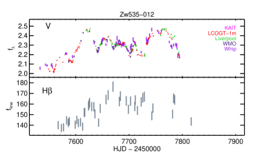
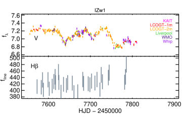
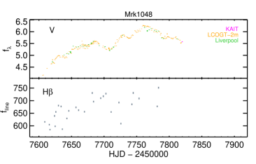
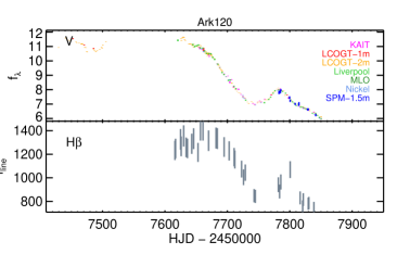
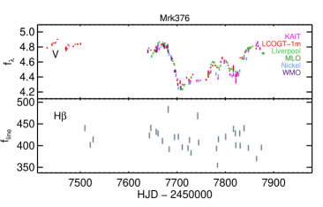
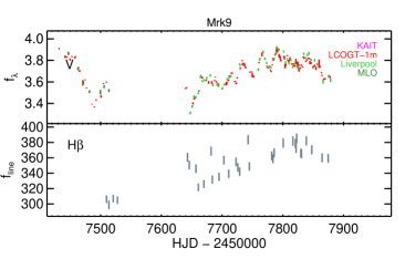
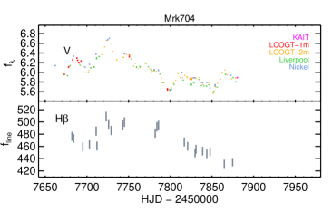
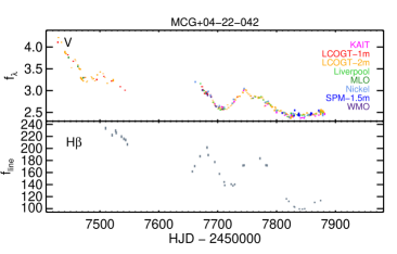
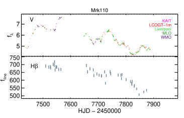
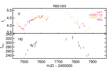
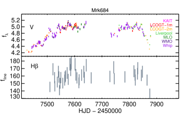
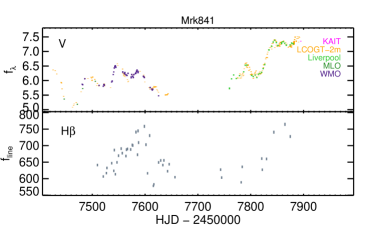
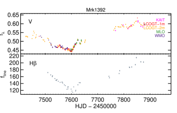
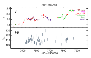
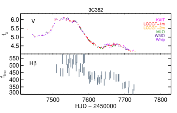
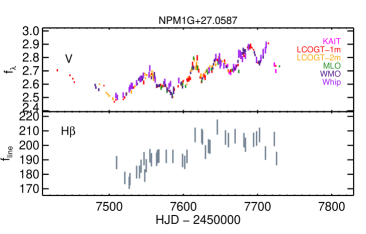
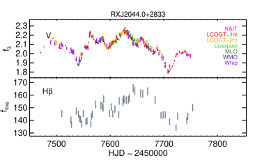
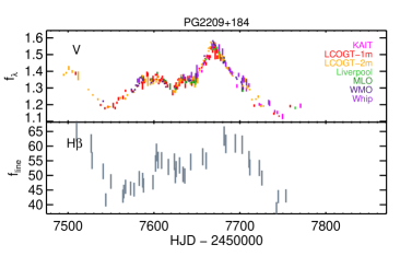
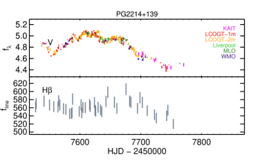
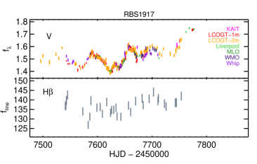
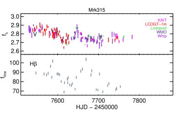
We used results from spectral decomposition to derive H $\beta$ emission-line light curves. The flexibility of the multicomponent modeling afforded us a number of ways to extract the H $\beta$ flux. In the spectral region near the H $\beta$ line, sources with strong Fe II emission were subjected to substantial degeneracy of spectral decomposition that could result in, from night to night, instability in model fitting in terms of how much flux gets assigned to the different model components. This instability results in additional noise in the H $\beta$ light curve. To minimize the noise due to degeneracy from spectral fits, we used a version of the decomposed model spectra where only the AGN and stellar continuum components have been removed. This version consisted of the residuals of all present emission lines after continuum subtraction. We then selected a corresponding extraction window free of other emission lines for the calculation of H $\beta$ flux (see Table 5). A different way to extract H $\beta$ flux is to use a version of the decomposed model spectra that only contained H $\beta$ broad and narrow components, with other emission-line components as well as the AGN and stellar continua removed. The resulting H $\beta$ light curves computed from the two methods were very similar for objects that have relatively clean H $\beta$ spectral regions, but those for the emission-line residual versions were less noisy for objects with more complex line profiles within the H $\beta$ spectral region. The final H $\beta$ light-curve measurements for the full sample are presented in Table 6. The light curves for the $V$ band and H $\beta$ are shown in . The rest of the emission-line features will be presented in a forthcoming paper.

Table 5: Emission-Line Extraction Windows in Å (observed frame),

F_{\rm var}

, and [O III] Excess Scatter

Object	H $\beta$	$F_{\rm var}$	[O III]	$\sigma_{\mathrm{[O~{}\textsc{iii}]}}$
Zw 535 $-$ 012	5018 $-$ 5181	0.050	5220 $-$ 5270	0.016
I Zw 1	5099 $-$ 5199	0.044	5263 $-$ 5337	0.054
Mrk 1048	5002 $-$ 5153	0.071	5200 $-$ 5252	0.004
Ark 120	4931 $-$ 5102	0.195	5143 $-$ 5200	0.043
Mrk 376	5069 $-$ 5201	0.064	5259 $-$ 5322	0.016
Mrk 9	5007 $-$ 5127	0.069	5179 $-$ 5241	0.016
Mrk 704	4945 $-$ 5059	0.046	5126 $-$ 5192	0.015
MCG $+$ 04 $-$ 22 $-$ 042	4986 $-$ 5079	0.268	5149 $-$ 5203	0.012
Mrk 110	4985 $-$ 5120	0.083	5161 $-$ 5208	0.015
RBS 1303	5001 $-$ 5136	0.081	5185 $-$ 5251	0.019
Mrk 684	5032 $-$ 5131	0.058	5209 $-$ 5262	0.048
Mrk 841	4949 $-$ 5120	0.073	5167 $-$ 5218	0.006
Mrk 1392	4958 $-$ 5108	0.173	5165 $-$ 5212	0.007
SBS 1518 $+$ 593	5191 $-$ 5310	0.051	5369 $-$ 5428	0.024
3C 382	5030 $-$ 5226	0.142	5268 $-$ 5342	0.067
NPM1G $+$ 27.0587	5092 $-$ 5246	0.051	5289 $-$ 5352	0.024
RXJ 2044.0 $+$ 2833	5040 $-$ 5187	0.055	5240 $-$ 5276	0.019
PG 2209 $+$ 184	5147 $-$ 5280	0.122	5329 $-$ 5387	0.052
PG 2214 $+$ 139	5110 $-$ 5260	0.028	5307 $-$ 5355	0.024
RBS 1917	5111 $-$ 5261	0.028	5231 $-$ 5444	0.016
Mrk 315	5002 $-$ 5111	0.109	5174 $-$ 5236	0.016

Table 6: H

\beta

Light Curve Data

Object	HJD	$f$	$\delta_{f}$ (stat)	$\delta_{f}$ (modified)
Mrk 110	7509.74	690.6	0.76	10.47
Mrk 110	7520.75	683.9	0.94	10.38
Mrk 110	7526.73	686.3	0.96	10.42
Mrk 110	7527.73	678.7	0.93	10.30
Mrk 110	7536.71	701.7	1.10	10.67
Mrk 110	7540.71	695.0	1.05	10.56
Mrk 110	7541.71	717.2	1.39	10.93
Mrk 110	7543.72	665.7	1.34	10.15
Mrk 110	7546.72	685.8	1.13	10.43
Mrk 110	7549.69	683.1	1.35	10.41

Note. — Dates are listed as HJD $-$ 2450000. Units for emission-line flux $f$ are in 10^-15 erg s^-1 cm^-2. The original $\delta_{f}$ represents the photon-counting errors on the flux measurement, while the modified $\delta_{f}$ incorporates the spectral scaling uncertainties from [O III] scatter. This table is published in its entirety in machine-readable format on the online version of the journal. Sample entries are shown here for guidance regarding the table’s form and content.

To account for the residual uncertainties from spectral scaling, we computed the excess variance in the [O III] light curve for each AGN as the additional uncertainty term. We then combined this excess variance term with the statistical error in quadrature such that

\delta_{f}^{2}\mathrm{(modified)}=\delta^{2}_{f}\mathrm{(stat)}+(f\times\sigma_{\mathrm{[O~{}\textsc{iii}]}})^{2}\quad.

(3)

Both the statistical and the modified errors are listed in Table 6. Following Bentz et al. (2009a), we compute the variability statistics $F_{\rm var}$ for each light curve and found that it ranges from 0.028 to 0.268, with a median of 0.069 (see Table 5). Almost a third of our sample (3C 382, Ark 120, MCG $+$ 04 $-$ 22 $-$ 042, Mrk 1392, Mrk 315, and PG 2209 $+$ 184) exhibit strong variability in the H $\beta$ light curves with $F_{\rm var}>0.1$ . Among the rest of the sample, a few galaxies (such as Zw 535 $-$ 012, Mrk 110, Mrk 841, RBS 1303, and RXJ2044.0 $+$ 2833) still display discernible variability for plausible lag determination even if the signal is diluted by large error bars or outliers.

5.1 Integrated H $\beta$ Lags

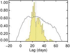
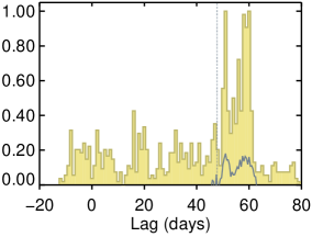
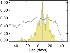
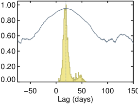
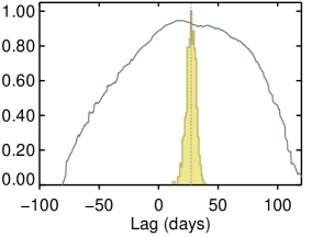
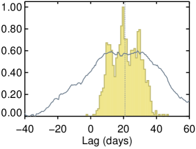
Following White & Peterson (1994), Peterson et al. (2004) and others, cross-correlation was employed to determine the delay in the integrated H $\beta$ line signal relative to that from the $V$ -band continuum from the photometric campaign. We chose to adopt the interpolated cross-correlation function (ICCF; e.g., Peterson et al., 1998) method. Given a lag range that represents reasonable bounds of the expected lag, the cross-correlation function (CCF) between the two light curves is computed at every time lag $\tau$ at 0.5 day intervals via

F_{\rm CCF}(\tau)=\frac{1}{N-1}\sum_{i=1}^{N}\frac{[L(t_{i})-\bar{L}][C(t_{i}-\tau)-\bar{C}]}{\sigma_{C}\sigma_{L}}\quad,

(4)

where $\bar{L}$ ( $\bar{C}$ ) and $\sigma_{L}$ ( $\sigma_{C}$ ) are the mean and standard deviation of the emission-line (continuum) time series, respectively.

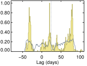
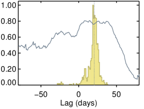
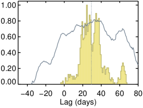
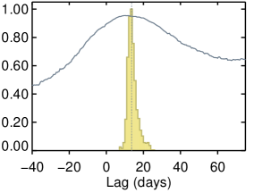
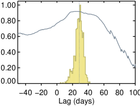
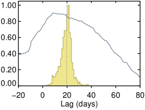
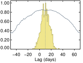
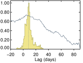
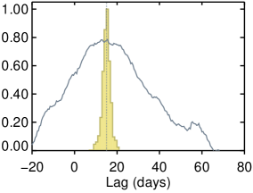
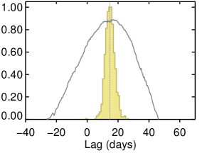
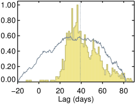
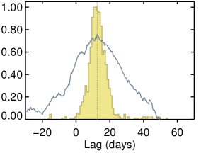
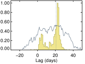
Two lag measures are computed: $\tau_{\rm peak}$ , the lag at the peak of the CCF, and $\tau_{\rm cen}$ , the centroid of the CCF for all points in the CCF above a predetermined threshold value (80% of the peak CCF value). We adopt the latter for the subsequent analysis. For error analysis, we employed the Monte Carlo flux randomization method and repeated the CCF calculation for 10³ realizations, building up distributions of correlation measurements. The median and $\pm$ 1 $\sigma$ widths of the cross-correlation centroid distributions (CCCD) were then adopted as the final lag measurements, and their associated uncertainties as shown in .

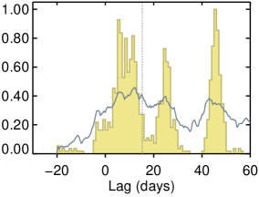
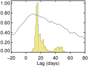
5.2 Assessment of Cross-Correlation Reliability

In any RM campaign, it is expected that some AGN will yield highly robust measurements of reverberation lag, thanks to strong variability and high-quality data, while other objects may exhibit little or no evidence for correlated variability between the continuum and emission-line light curves. This can occur as a result of observational factors including low S/N or poor temporal sampling, or factors intrinsic to the AGN including low variability amplitude or low responsivity of the emission line to variations in the ionizing continuum. There is not necessarily a clear demarcation between reliable and unreliable lag measurements, and a variety of methods have been used to assess the significance or quality of lag detections (e.g., Grier et al., 2017). In some cases, a simple threshold value of the correlation strength $r_{\mathrm{max}}$ is used, but $r_{\mathrm{max}}$ alone is not necessarily a good indicator of correlation significance for red-noise light curves. An alternative method is to employ null-hypothesis testing to determine the probability that two uncorrelated red-noise light curves having the same S/N and cadence as the data would yield an $r_{\mathrm{max}}$ at least as strong as the observed value. Such methods have been employed for analysis of multiwavelength continuum correlations in AGN (e.g., Uttley et al., 2003; Arévalo et al., 2008; Chatterjee et al., 2008), but until recently have rarely been employed to assess broad-line reverberation lags (Penton et al., 2021; Li et al., 2021). Our method will be presented in detail by Guo et al. (in prep.), and we provide a brief description here.

We first generated light curves according to the damped random walk (DRW) model with the Python software CARMA¹¹1https://github.com/brandonckelly/carma_pack (Kelly et al., 2009, 2014). The DRW model provides an adequate description of ultraviolet/optical variabilities in AGN, though with plausible deviations on short (McHardy et al., 2006; Mushotzky et al., 2011; Kasliwal et al., 2015; Smith et al., 2018) or long (MacLeod et al., 2010; Guo et al., 2017) timescales. Each simulated light curve represents a segment randomly selected from a 100-times longer light curve predicted from the same DRW model fitted to the observed light curve. We resampled each mock light curve to have the same cadence as the real observations and added Gaussian random noise based on the S/N of the data, creating $10^{3}$ realizations of each light curve. Cross-correlation measurements were then carried out using the simulated data to determine the distribution of $r_{\mathrm{max}}$ values that would be obtained for uncorrelated light curves. A two-way simulation was performed — that is, we calculated the CCF between the real continuum and each simulated emission-line light curve for the first 500 simulations, and then the opposite way for the rest of the realizations.

We measured the CCF for all the simulations, using the same lag search range employed for each AGN, and counted, out of 10³, the number of positive lags ( $\tau>0$ ) with peak values $r_{\rm max}$ higher than our observed $r_{\rm max}$ . The resulting fraction represents the probability that a correlation signal found between two uncorrelated light curves would exceed the correlation signal of the data. This derived $p$ -value, denoted $p(r_{\mathrm{max}})$ , thus provides an indicator of the robustness of our lag detections given the observed $r_{\mathrm{max}}$ and the observed properties of the light curves including S/N, cadence, and duration.

We emphasize that the $p$ -values derived from this method are not false-positive probabilities, and they do not give a measure of the absolute “significance” of a lag detection. Strictly speaking, our $p$ -values simply give the probability that uncorrelated light curves having the same statistical properties as the data would give a cross-correlation signal as strong as that seen in the data. Consequently, a smaller $p$ -value denotes a more robust and reliable detection of the correlation signal between two light curves. In general, for broad-line RM we have a strong prior that a reverberation signal is very likely to be present in the data, thus our null hypothesis of intrinsically uncorrelated light curves is an extreme and fairly unlikely scenario. We further emphasize that there is no strict cutoff between significant and insignificant lag detections by this method; the $p$ -value merely gives an indication of the relative degree of reliability between different measurements.

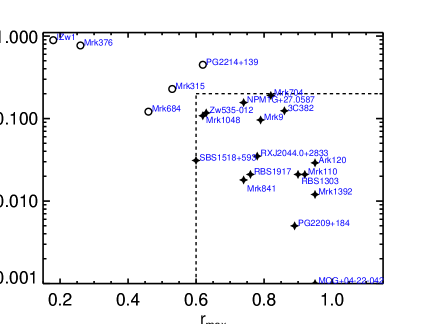
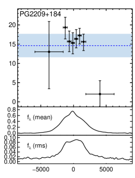
We assess the quality of our resulting lags based on these quantitative assessment indicators in Figure 11. As expected, there is an anticorrelation between $r_{\mathrm{max}}$ and $p(r_{\mathrm{max}})$ , but it is not a tight one-to-one relationship owing to the differences in S/N, sampling cadence, and variability amplitude among our sample. The results are consistent with the general expectation that the highest-quality light curves that exhibit clear correlated variability have high $r_{\rm max}$ and small $p(r_{\mathrm{max}})$ values. Considering these lag-assessment results, we conclude that 16 of the 21 AGN in our sample falling in the region $p(r_{\mathrm{max}})<0.2$ and $r_{\mathrm{max}}>0.6$ have correlations between continuum and H $\beta$ light curves that are sufficiently robust for the ensuing analyses (noting that they display a broad range of $p$ -values and thus range from highly robust to relatively weak detections of correlated variability), while we discard the remaining five objects from further analysis based on their low $r_{\mathrm{max}}$ and high $p$ -values. Based partly on visual inspection of the light-curve quality, our chosen $r_{\mathrm{max}}$ threshold is relatively conservative compare to those selected by other large surveys (e.g., minimum $r_{\mathrm{max}}$ = 0.45 by SDSS-RM; Grier et al., 2017). These $r_{\rm max}$ and $p(r_{\mathrm{max}})$ values, along with AGN luminosities and lag measurements $\tau_{\rm cen}$ in both observed and rest frames, are reported in Table 7. [Only the $r_{\rm max}$ and $p(r_{\mathrm{max}})$ are reported for the subsample of sources with unreliable lag measurements.]

Table 7: AGN Luminosity and H

\beta

Cross-Correlation Lag Results

		$\tau_{\rm cen}$	$\tau_{\rm peak}$	$\tau_{\rm cen}$	$\tau_{\rm peak}$
Object	$\lambda L_{\lambda}$ (5100 Å)	Observed Frame		Rest Frame		$r_{\rm max}$	$p(r_{\mathrm{max}})$	BLR Kinematics
	(10⁴³ erg s^-1)	(days)	(days)	(days)	(days)
Zw 535 $-$ 012	4.9 $\pm$ 0.7	21.3 ${}_{-4.8}^{+8.5}$	22.0 ${}_{-8.0}^{+6.5}$	20.3 ${}_{-4.6}^{+8.1}$	21.0 ${}_{-7.6}^{+6.2}$	0.63	0.12	Infalling
Mrk 1048	9.5 $\pm$ 1.8	7.8 ${}_{-9.8}^{+10.1}$	10.0 ${}_{-13.0}^{+9.0}$	7.4 ${}_{-9.4}^{+9.7}$	9.6 ${}_{-12.5}^{+8.6}$	0.62	0.11	Infalling
Ark 120	9.2 $\pm$ 3.4	19.3 ${}_{-4.6}^{+6.1}$	20.5 ${}_{-4.5}^{+5.5}$	18.7 ${}_{-4.5}^{+5.9}$	19.9 ${}_{-4.4}^{+5.3}$	0.95	0.03	Ambiguous
Mrk 9	5.6 $\pm$ 0.4	20.3 ${}_{-7.6}^{+4.2}$	15.0 ${}_{-7.0}^{+12.0}$	19.5 ${}_{-7.3}^{+4.1}$	14.4 ${}_{-6.7}^{+11.5}$	0.79	0.10	Ambiguous
Mrk 704	6.2 $\pm$ 0.6	29.8 ${}_{-10.3}^{+10.4}$	34.5 ${}_{-19.5}^{+5.5}$	28.9 ${}_{-10.0}^{+10.2}$	33.5 ${}_{-18.9}^{+5.3}$	0.82	0.19	Infalling
MCG $+$ 04 $-$ 22 $-$ 042	1.6 $\pm$ 0.4	13.7 ${}_{-1.9}^{+2.5}$	10.5 ${}_{-1.0}^{+3.0}$	13.3 ${}_{-1.8}^{+2.4}$	10.2 ${}_{-1.0}^{+2.9}$	0.95	0.00	Symmetric
Mrk 110	7.2 $\pm$ 1.7	28.8 ${}_{-5.2}^{+4.4}$	22.5 ${}_{-4.0}^{+7.5}$	27.8 ${}_{-5.1}^{+4.3}$	21.7 ${}_{-3.9}^{+7.2}$	0.92	0.02	Symmetric
RBS 1303	2.4 $\pm$ 0.4	19.4 ${}_{-4.5}^{+3.6}$	13.5 ${}_{-4.5}^{+7.5}$	18.7 ${}_{-4.3}^{+3.4}$	13.0 ${}_{-4.3}^{+7.2}$	0.90	0.02	Outflowing
Mrk 841	6.7 $\pm$ 0.9	11.7 ${}_{-3.7}^{+5.0}$	9.0 ${}_{-2.0}^{+5.0}$	11.2 ${}_{-3.5}^{+4.8}$	8.7 ${}_{-1.9}^{+4.8}$	0.74	0.02	Infalling
Mrk 1392	1.6 $\pm$ 0.6	27.6 ${}_{-4.0}^{+3.6}$	17.5 ${}_{-2.0}^{+3.0}$	26.7 ${}_{-3.9}^{+3.5}$	16.9 ${}_{-1.9}^{+2.9}$	0.95	0.01	Symmetric
SBS 1518 $+$ 593	10.6 $\pm$ 1.0	21.7 ${}_{-9.5}^{+9.0}$	22.0 ${}_{-11.0}^{+9.5}$	20.1 ${}_{-8.9}^{+8.4}$	20.4 ${}_{-10.2}^{+8.8}$	0.60	0.03	Infalling
3C 382	15.0 $\pm$ 3.1	10.0 ${}_{-7.1}^{+7.2}$	6.5 ${}_{-7.0}^{+13.5}$	9.5 ${}_{-6.7}^{+6.8}$	6.1 ${}_{-6.6}^{+12.8}$	0.86	0.12	Symmetric
NPM1G $+$ 27.0587	10.9 $\pm$ 1.0	8.5 ${}_{-4.7}^{+5.0}$	7.5 ${}_{-4.0}^{+6.5}$	8.0 ${}_{-4.5}^{+4.7}$	7.1 ${}_{-3.8}^{+6.1}$	0.74	0.16	Infalling
RXJ 2044.0 $+$ 2833	5.3 $\pm$ 0.5	15.1 ${}_{-2.0}^{+1.7}$	15.0 ${}_{-3.5}^{+4.0}$	14.4 ${}_{-1.9}^{+1.6}$	14.3 ${}_{-3.3}^{+3.8}$	0.78	0.04	Infalling
PG 2209 $+$ 184	2.3 $\pm$ 0.6	14.6 ${}_{-3.1}^{+3.0}$	16.0 ${}_{-5.0}^{+3.0}$	13.7 ${}_{-2.9}^{+2.8}$	15.0 ${}_{-4.7}^{+2.8}$	0.89	0.01	Ambiguous
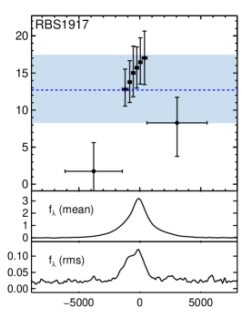
RBS 1917	4.9 $\pm$ 0.5	12.7 ${}_{-4.1}^{+4.6}$	12.5 ${}_{-3.5}^{+4.5}$	11.9 ${}_{-3.9}^{+4.3}$	11.7 ${}_{-3.3}^{+4.2}$	0.76	0.02	Outflowing
I Zw 1	28.5 $\pm$ 4.0	$\cdots$	$\cdots$	$\cdots$	$\cdots$	0.18	0.89	$\cdots$
Mrk 376	17.6 $\pm$ 1.8	$\cdots$	$\cdots$	$\cdots$	$\cdots$	0.26	0.77	$\cdots$
Mrk 684	8.3 $\pm$ 0.9	$\cdots$	$\cdots$	$\cdots$	$\cdots$	0.46	0.12	$\cdots$
PG 2214 $+$ 139	21.2 $\pm$ 1.3	$\cdots$	$\cdots$	$\cdots$	$\cdots$	0.62	0.45	$\cdots$
Mrk 315	3.2 $\pm$ 0.4	$\cdots$	$\cdots$	$\cdots$	$\cdots$	0.53	0.23	$\cdots$

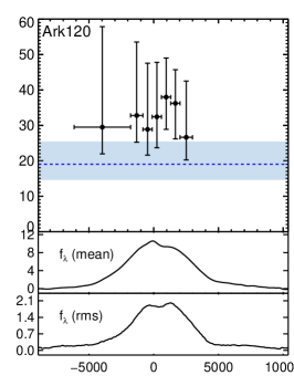
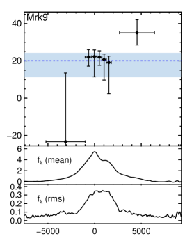
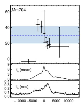
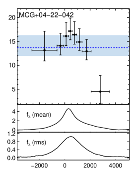
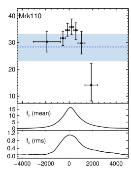
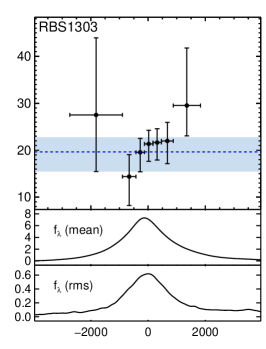
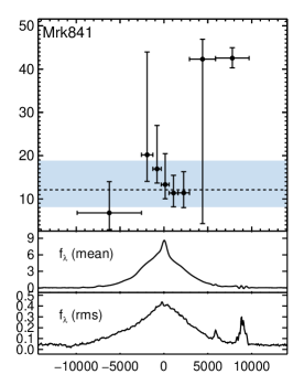
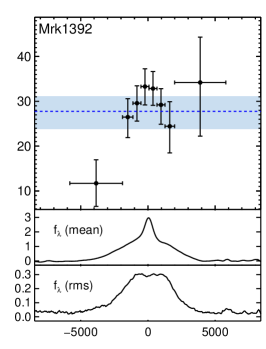
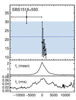
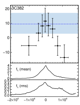
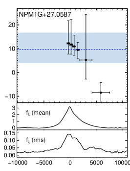
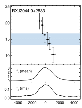
5.3 Velocity-Resolved H $\beta$ Lags

To obtain velocity-resolved reverberation results as a means to probe the kinematics of the BLR gas, we used CCF to compute lag measurements for individual velocity segments of the emission line. Our procedure follows that described by Bentz et al. (2009b), Denney et al. (2009), and Grier et al. (2013), and is detailed below.

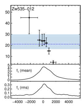
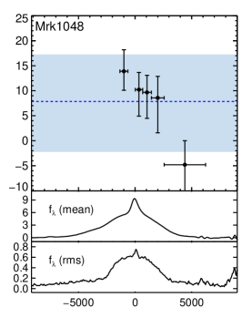
To verify the effect of binning on the apparent BLR kinematics, we divided the broad H $\beta$ component into eight bins via two different schemes: (i) bins of equal rms flux, and (ii) bins of equal velocity width. In the first approach, we initially determined the total rms flux from integrating the H $\beta$ line in the e-rms spectrum. Then we established velocity bins such that the rms flux within each bin would equal one-eighth of the total flux. There are some exceptions in the cases where the red wing of the rms profile suffered from significant noise and the last bin was thus truncated at the red line wing. In the second approach, bins are divided evenly across the width of the line in velocity space. In either binning scheme, light curves were computed from each bin of the continuum-subtracted H $\beta$ profile and lags were measured against the $V$ -band continuum light curve. Resulting lags from the two binning schemes generally agree in the line’s core where the S/N is high; minor disagreement is found in the noisy line wings of some sources. For clarity, we adopt the first scheme (equal-rms-flux binning) and show the resulting for each AGN with robust lag in Figure 12 and in Table 8.

Table 8: Velocity-Resolved Lags

Object	Velocity Bin	$\tau_{\rm cen}$
	(km s^-1)	(days)
Mrk110	-1910 $\pm$ 2324	30.34 ${}^{+3.90}_{-3.86}$
Mrk110	-539 $\pm$ 417	31.66 ${}^{+2.60}_{-2.79}$
Mrk110	-151 $\pm$ 357	34.66 ${}^{+2.57}_{-2.26}$
Mrk110	205 $\pm$ 357	35.83 ${}^{+3.04}_{-2.85}$
Mrk110	563 $\pm$ 357	34.65 ${}^{+2.79}_{-3.48}$
Mrk110	1040 $\pm$ 596	29.80 ${}^{+4.45}_{-4.04}$
Mrk110	1874 $\pm$ 1073	14.12 ${}^{+8.08}_{-5.93}$

Note. — This table is published in its entirety in machine-readable format on the online version of the journal. Sample entries are shown here for guidance regarding the table’s form and content.

5.4 Implications for BLR Kinematics

The velocity-resolved lags allow us to make simple qualitative inferences about the BLR geometry and kinematics from the transfer-function models (e.g., Welsh & Horne, 1991; Horne et al., 2004; Bentz et al., 2009b). Qualitatively, symmetric velocity-resolved structure around zero velocity is consistent with either Keplerian, disk-like rotation or random motion without net radial inflow or outflow over an extended BLR. In such a case, the high-velocity wings exhibit the shortest lags because the highest rotation speeds correspond to material orbiting closest to the central black hole. Radially infalling gas produces an asymmetric pattern displaying longer lags at the high-velocity blue wing, while the opposite is true in the case of outflow-dominated kinematics. We note that the presence of absorption, noise, or other geometric complexities may muddle these interpretations, which could be elucidated with direct modeling using forward-modeling codes such as CARAMEL in follow-up work (Villafaña et al., in prep.).

We find a diversity of among our sample symmetric (3C 382, MCG +04 $-$ 22 $-$ 042, Mrk 110, Mrk 1392), infalling (Mrk 1048, Mrk 704, Zw 535 $-$ 012, Mrk 841, RXJ 2044.0+2833, NPM1G $+$ 27.0587, SBS 1518+593), and outflowing (RBS 1303 and RBS 1917) . In the cases of Ark 120, Mrk 9, and PG 2209+184, the velocity-resolved structure appears flat across the H $\beta$ profile within the uncertainties, which may be difficult to describe with simple models. Whether these kinematics exhibit luminosity-dependent trends and how a subset of these results relate to other RM samples will be further examined in §6 and Appendix, respectively.

6 Black Hole Scaling Relations

6.1 AGN Radius–Luminosity Relationship

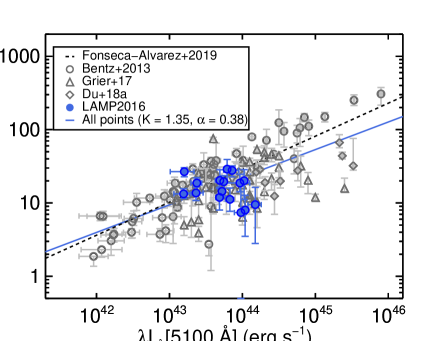
Here we compare our sample on the AGN radius–luminosity relationship with other RM samples from the literature Bentz et al. (2013); Grier et al. (2017); Du et al. (2018b) in Figure 13. The best-fit line from SDSS-RM for this relation is

\log(R_{\rm BLR}/{\rm ltday})=K+\alpha\log(\lambda L_{\lambda}(5100\,\AA)/10^{44}~{}{\rm erg~{}s}^{-1}),

(5)

with a median slope $\alpha$ = 0.45 and a median normalization $K$ = 1.46 Fonseca Alvarez et al. (2019). We computed the AGN luminosity $\lambda L_{\lambda}$ (5100 Å) based on the AGN continuum flux at 5100 Å as extracted from the decomposition of the mean spectrum. Luminosity distances were derived using the cosmology calculator ( $H_{0}=67.8$ km s^-1 Mpc^-1) provided by Wright (2006). All of our AGN fall within 0.5 dex of the radius–luminosity relation as defined by the literature points within the range of $\lambda L_{\lambda}$ (5100 Å) = $10^{43.5-44.4}$ erg s^-1. The best-fit line in the form of Equation 5 for all the data points combining our current work with those from the literature has a normalization $K$ = 1.35 and $\alpha$ = 0.38.

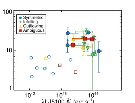
We further explore whether BLR kinematics might depend on AGN luminosity. Past work has shown that while inflow or outflow are indicated in a subset of AGN, the majority of H $\beta$ velocity-delay maps appear roughly symmetric with rotationally dominated kinematics (e.g., Bentz et al., 2009b, 2010b; Denney et al., 2010; Barth et al., 2011; Horne et al., 2021). The AGN with velocity-resolved reverberation detected to-date are mostly within the low-luminosity range [ $\lambda L_{\lambda}$ (5100 Å) = $10^{42-43.5}$ erg s^-1]. Our results add significantly to the existing number of sources having velocity-resolved measurements with $\lambda L_{\lambda}$ (5100 Å) $\approx 10^{44}$ erg s^-1. we illustrate the BLR kinematics via different colored symbols shown alongside those from the literature in Figure 14. No trend is seen between BLR kinematics and AGN luminosity either within our LAMP2016 sample or when combined with past results from the literature. It is plausible that the BLR shows time-dependent structural changes, from both the kinematic and the geometric points of view, and there may be a lag in its correlation with the of the AGN. The diversity in BLR kinematics found in our moderately high-luminosity sample appears consistent with that seen among AGN with super-Eddington accretion rates (e.g., Du et al., 2016b).

6.2 H $\beta$ Line Widths

Following the procedure outlined by Barth et al. (2015), we measured the line width of the broad H $\beta$ component from both the spectrally-decomposed mean spectrum and the rms spectrum. The mean spectrum constructed from the time-series data has a continuum level of zero with just residual noise from spectral fitting, but the continuum of the rms spectrum incorporates photon-counting errors in addition to residual noise. The noise continuum is removed after a simple linear fit before making line-width measurements.

We computed the line width using two separate parameters according to Peterson et al. (2004): the full width at half-maximum intensity (FWHM) of the line, and the line dispersion $\sigma_{\rm line}$ . The FWHM of a single-peaked line is defined as the difference between the wavelengths blueward and redward of the peak $P(\lambda)_{\rm max}$ that correspond to half of its height. A double-peaked line requires additional attention to defining $P(\lambda_{\rm blue,red})_{\rm max}$ for the blue and red peaks, respectively, and thus their corresponding wavelengths at half the maximum height, but otherwise the procedure in determining the difference between the resulting wavelengths is similar. As for $\sigma_{\rm line}$ (square root of the second moment of the H $\beta$ line profile), we adopted from Peterson et al. (2004) the following:

\sigma^{2}_{\rm line}(\lambda)=\langle\lambda^{2}\rangle-\lambda_{0}^{2}\quad,

(6)

where

\langle\lambda^{2}\rangle=\frac{\int\lambda^{2}P(\lambda)d\lambda}{\int P(\lambda)d\lambda}

(7)

and

\lambda_{0}=\frac{\int\lambda P(\lambda)d\lambda}{\int P(\lambda)d\lambda}\quad.

(8)

In each of these calculations, we also varied the endpoints of the H $\beta$ extraction window randomly within $\pm 5$ Å ten times in order to account for uncertainties brought about by the precise choice of the H $\beta$ spectral limits. The resulting line-width measurement is the mean from these ten trials.

For error analysis associated with the measured width parameters, we undertook a Monte Carlo bootstrapping procedure and simulated 100 realizations of the mean and rms spectra, respectively, based on random subset sampling of the existing nightly spectra. For a source with $n$ epochs of observations, we simulate new mean and rms spectra of the broad H $\beta$ component from combining $n$ randomly-drawn time-series spectra with repetition allowed. We repeated our measurement of the FWHM and $\sigma_{\rm line}$ on these new spectra, where the means and the standard deviations of the resulting distributions were taken as the line widths and their corresponding uncertainties, respectively.

The final line-width measurements are corrected for instrumental broadening subtracted in quadrature from the observed line width $\Delta\lambda_{\rm obs}$ :

\Delta\lambda^{2}_{\rm intrinsic}=\Delta\lambda^{2}_{\rm obs}-\Delta\lambda^{2}_{\rm inst}\quad.

(9)

Given that we used the same blue-side spectral setup as the LAMP2011 campaign, we adopt from Barth et al. (2015) the instrumental FWHM of 380 km s^-1 and dispersion $\sigma_{\rm inst}\approx 162$ km s^-1 for our small corrections. The resulting FWHM and $\sigma_{\rm line}$ measured from both the mean and the e-rms spectra are presented in Table 9.

Table 9: Rest-Frame Line Widths of the Broad H

\beta

Component

	Mean				rms
Object	FWHM		$\sigma_{\rm line}$		FWHM		$\sigma_{\rm line}$
Zw 535 $-$ 012	2705 $\pm$	33	1474 $\pm$	28	2005 $\pm$	80	1259 $\pm$	112
I Zw 1	2187 $\pm$	920	1644 $\pm$	102	2665 $\pm$	700	916 $\pm$	165
Mrk 1048	4830 $\pm$	80	1840 $\pm$	58	4042 $\pm$	406	1726 $\pm$	76
Ark 120	5656 $\pm$	44	2125 $\pm$	41	4765 $\pm$	84	1882 $\pm$	42
Mrk 376	10055 $\pm$	341	2662 $\pm$	38	14438 $\pm$	1439	3633 $\pm$	210
Mrk 9	3751 $\pm$	71	1555 $\pm$	68	3159 $\pm$	144	1326 $\pm$	69
Mrk 704	8597 $\pm$	448	2002 $\pm$	63	8597 $\pm$	448	2009 $\pm$	102
MCG $+$ 04 $-$ 22 $-$ 042	2658 $\pm$	57	1141 $\pm$	39	2120 $\pm$	39	977 $\pm$	29
Mrk 110	2048 $\pm$	13	1203 $\pm$	32	2052 $\pm$	100	1314 $\pm$	69
RBS 1303	2286 $\pm$	21	1243 $\pm$	26	1738 $\pm$	113	1292 $\pm$	156
Mrk 684	2174 $\pm$	33	1216 $\pm$	74	2391 $\pm$	632	2010 $\pm$	773
Mrk 841	7073 $\pm$	311	2139 $\pm$	55	7452 $\pm$	660	2278 $\pm$	96
Mrk 1392	4267 $\pm$	25	1635 $\pm$	13	3690 $\pm$	138	1501 $\pm$	38
SBS 1518 $+$ 593	3312 $\pm$	24	1782 $\pm$	21	4656 $\pm$	1692	2249 $\pm$	255
3C 382	7772 $\pm$	54	4218 $\pm$	67	13926 $\pm$	2337	5616 $\pm$	97
NPM1G $+$ 27.0587	3501 $\pm$	28	1683 $\pm$	42	2893 $\pm$	177	1735 $\pm$	136
RXJ 2044.0 $+$ 2833	2196 $\pm$	31	989 $\pm$	32	2047 $\pm$	72	870 $\pm$	50
PG 2209 $+$ 184	4045 $\pm$	34	1573 $\pm$	40	3247 $\pm$	88	1353 $\pm$	64
PG 2214 $+$ 139	5133 $\pm$	17	1947 $\pm$	55	4867 $\pm$	473	1984 $\pm$	90
RBS 1917	2399 $\pm$	11	1180 $\pm$	50	1653 $\pm$	287	851 $\pm$	154
Mrk 315	3097 $\pm$	252	1824 $\pm$	67	3411 $\pm$	1438	2031 $\pm$	260

Note. — All line-width measurements are in km s^-1.

6.3 Virial Black Hole Masses

The mass of a black hole may be determined most robustly using dynamical modeling codes such as CARAMEL (e.g., Pancoast et al., 2011). Nonetheless, virial estimates are useful within uncertainties that depend on the BLR geometry. The black hole mass and its associated uncertainty are computed and propagated from the virial equation

M_{\rm virial}=f\frac{c\tau v^{2}}{G}\quad,

(10)

	$\displaystyle\sigma_{M}=\sqrt{\left(\frac{\delta M}{\delta\tau}\sigma_{\tau}\right)^{2}+\left(\frac{\delta M}{\delta v}\sigma_{v}\right)^{2}}$
	$\displaystyle=M\sqrt{\left(\frac{\sigma_{\tau}}{\tau}\right)^{2}+4\left(\frac{\sigma_{v}}{v}\right)^{2}}\quad,$		(11)

where $f$ is the scaling factor that depends on the geometry and kinematics of the BLR, $c$ is the speed of light, $\tau\pm\sigma_{\tau}$ is the time delay with uncertainties, $v\pm\sigma_{v}$ is the velocity of the BLR gas with uncertainties as measured by the line width, and $G$ is the gravitational constant. The empirically fitted virial factor from Woo et al. (2015) is consistent with that from CARAMEL dynamical modeling Pancoast et al. (2014b), so we have adopted for our black hole mass calculations $\langle f\rangle=10^{0.65}=4.47$ from Woo et al. (2015), $\tau=\tau_{\mathrm{cen}}$ , and $v=\sigma_{\mathrm{line}}$ (rms) to facilitate comparisons with other studies. We present both the virial products $c\tau_{\rm cen}\sigma^{2}_{\rm line}/G$ and the derived $f$ -dependent black hole masses in Table 10. Comparisons of our results to existing prior black hole mass measurements for several sources can be found in Appendix. Overall, we find agreements between our measurements and those from the literature within uncertainties.

Table 10: Virial Products and Derived BH Masses

Object	$c\tau_{\rm cen}\sigma^{2}_{\rm line}/G$	$M_{\rm BH}^{\dagger}$
	(10 ${}^{7}~{}M_{\odot}$ )	(10 ${}^{8}~{}M_{\odot}$ )
Zw 535 $-$ 012	0.85 ${}^{+0.36}_{-0.18}$	0.38 ${}^{+0.16}_{-0.08}$
Mrk 1048	0.50 ${}^{+0.60}_{-0.64}$	0.22 ${}^{+0.27}_{-0.29}$
Ark 120	1.62 ${}^{+0.55}_{-0.38}$	0.73 ${}^{+0.25}_{-0.17}$
Mrk 9	0.91 ${}^{+0.21}_{-0.41}$	0.41 ${}^{+0.09}_{-0.18}$
Mrk 704	2.30 ${}^{+0.91}_{-0.79}$	1.03 ${}^{+0.41}_{-0.36}$
MCG $+$ 04 $-$ 22 $-$ 042	0.34 ${}^{+0.07}_{-0.05}$	0.15 ${}^{+0.03}_{-0.02}$
Mrk 110	0.77 ${}^{+0.14}_{-0.15}$	0.35 ${}^{+0.06}_{-0.07}$
RBS 1303	0.57 ${}^{+0.09}_{-0.12}$	0.25 ${}^{+0.04}_{-0.06}$
Mrk 841	1.04 ${}^{+0.58}_{-0.35}$	0.47 ${}^{+0.26}_{-0.16}$
Mrk 1392	1.40 ${}^{+0.17}_{-0.20}$	0.63 ${}^{+0.08}_{-0.09}$
SBS 1518 $+$ 593	1.23 ${}^{+0.49}_{-0.56}$	0.55 ${}^{+0.22}_{-0.25}$
3C 382	3.12 ${}^{+2.51}_{-2.19}$	1.39 ${}^{+1.12}_{-0.98}$
NPM1G $+$ 27.0587	0.51 ${}^{+0.37}_{-0.30}$	0.23 ${}^{+0.16}_{-0.13}$
RXJ 2044.0 $+$ 2833	0.27 ${}^{+0.04}_{-0.04}$	0.12 ${}^{+0.02}_{-0.02}$
PG 2209 $+$ 184	0.66 ${}^{+0.14}_{-0.14}$	0.29 ${}^{+0.06}_{-0.06}$
RBS 1917	0.32 ${}^{+0.12}_{-0.12}$	0.14 ${}^{+0.06}_{-0.05}$

Note. — ^†Assuming $f=4.47$ Woo et al. (2015).

7 Conclusions

We present the first results from our 100-night LAMP2016 campaign where we monitored a sample of 21 luminous Seyfert 1 nuclei with AGN luminosity $\lambda L_{\lambda}$ (5100 Å) $\approx 10^{44}$ erg s^-1 during April 2016 – May 2017 at Lick Observatory. Our analysis here provided the H $\beta$ emission-line light curves and integrated H $\beta$ lag detections measured against $V$ -band continuum photometric light curves for the full sample. We further assessed the significance of the lag determinations, and computed, for a subset of sources with good-quality lags, their velocity-resolved reverberations, inferred BLR kinematics, broad H $\beta$ line widths, and virial black hole mass estimates.

The unusually rainy weather at Mount Hamilton during the winter months of 2016–2017 hampered our ability to monitor the variability of our AGN as closely as would have been ideal, leaving large gaps in several of our emission-line light curves. Consequently, we were not able to measure reliable lags for six of our AGN owing to inadequate light curves. Our overall results nearly double the number of existing velocity-resolved lag measurements, particularly at the moderately high-luminosity regime among previous reverberation-mapped samples, and revealed a diversity of BLR gas kinematics. depend on other properties of the accreting black holes. Follow-up direct dynamical modeling work will shed light on the detailed kinematics and provide robust dynamical black hole masses to help further calibrate widely-adopted black hole scaling relations.

We thank the anonymous referee for thoughtful comments and great suggestions that significantly improved this manuscript. We are grateful to M. Fausnaugh for offering help with their mapspec code used to test different spectral scaling of our Shane/Kast data, and M. Bentz for providing her table of values for the radius–luminosity relationship. We acknowledge the following individuals for their time and effort contributed to the Lick observing campaign: (Shane) Zachary Parsons, Estefania Padilla Gonzalez, Noah Rivera, Cristilyn Gardner, Jake Haslemann, Sean Lewis, and Ellen Glad; (Nickel) Nick Choksi, Sameen Yunus, Jeff Molloy, Andrew Rikhter, and Haynes Stephens. Photometric data collection at MLO was supported by NSF grant AST-1210311; we thank Robert Quimby, Emma Lee, Joseph Tinglof, Eric McLaughlin, Amy Igarashi, and Tariq Johnson for assistance with these observations. We are deeply grateful to the UCO/Lick staff for help with scheduling and supporting the observations. Research at Lick Observatory is partially supported by a generous gift from Google. The Kast red CCD detector upgrade, led by B. Holden, was made possible by the Heising-Simons Foundation, William and Marina Kast, and the University of California Observatories. KAIT and its ongoing operation were made possible by donations from Sun Microsystems, Inc., the Hewlett-Packard Company, AutoScope Corporation, Lick Observatory, the NSF, the University of California, the Sylvia & Jim Katzman Foundation, and the TABASGO Foundation. Data presented herein were obtained using the UCI Remote Observing Facility, made possible by a generous gift from John and Ruth Ann Evans. Research at UC Irvine has been supported by NSF grants AST-1412693 and AST-1907208. V.U acknowledges funding support from the University of California Riverside’s Chancellor’s Postdoctoral Fellowship and NASA Astrophysics Data Analysis Program Grant #80NSSC20K0450. Her work was conducted in part at the Aspen Center for Physics, which is supported by NSF grant PHY-1607611; she thanks the Center for its hospitality during the “Astrophysics of Massive Black Holes Merger" workshop in June and July 2018. T.T. acknowledges support by the Packard Foundation through a Packard research fellowship. V.N.B. and I.S. gratefully acknowledge assistance from NSF Research at Undergraduate Institutions (RUI) grants AST-1312296 and AST-1909297. Note that findings and conclusions do not necessarily represent views of the NSF. G.C. acknowledges NSF support under grant AST-1817233. J.H.W. acknowledges the funding from the Basic Science Research Program through the National Research Foundation of Korean Government (NRF-2021R1A2C3008486). A.V.F.’s group at U.C. Berkeley is grateful for support from the TABASGO Foundation, the Christopher R. Redlich Fund, the Miller Institute for Basic Research in Science (in which he is a Miller Senior Fellow), and many individual donors. K.H. acknowledges support from STFC grant ST/R000824/1. We acknowledge the generous support of Marc J. Staley, whose fellowship partly funded B.E.S. whilst contributing to the work presented herein as a graduate student. I.S. acknowledges support from the Deutsche Forschungsgemeinschaft (DFG, German Research Foundation) under Germany’s Excellence Strategy — EXC 2121 "Quantum Universe" — 390833306. Research by S.V. is supported by NSF grants AST–1813176 and AST-2008108. This work makes use of observations from the LCOGT network. The Liverpool Telescope is operated on the island of La Palma by Liverpool John Moores University in the Spanish Observatorio del Roque de los Muchachos of the Instituto de Astrofisica de Canarias with financial support from the UK Science and Technology Facilities Council. Based on observations acquired at the Observatorio Astronómico Nacional in the Sierra San Pedro Mártir (OAN-SPM), Baja California, México, we thank the daytime and night support staff at the OAN-SPM for facilitating and helping obtain our observations. Some of the data used in this paper were acquired with the RATIR instrument, funded by the University of California and NASA Goddard Space Flight Center, and the 1.5-meter Harold L. Johnson telescope at the Observatorio Astronómico Nacional on the Sierra de San Pedro Mártir, operated and maintained by the Observatorio Astronómico Nacional and the Instituto de Astronomía of the Universidad Nacional Autónoma de México. Operations are partially funded by the Universidad Nacional Autónoma de México (DGAPA/PAPIIT IG100414, IT102715, AG100317, IN109418, IG100820, and IN105921). We acknowledge the contribution of Leonid Georgiev and Neil Gehrels to the development of RATIR. This research was made possible through the use of the AAVSO Photometric All-Sky Survey (APASS), funded by the Robert Martin Ayers Sciences Fund and NSF grant AST-1412587 and contributed by observers worldwide. We acknowledge the use of The AGN Black Hole Mass Database as a compilation of some of the reverberation mapped black hole masses prior to 2015 Bentz & Katz (2015). This research has made use of the NASA/IPAC Extragalactic Database (NED), which is operated by the Jet Propulsion Laboratory, California Institute of Technology, under contract with the National Aeronautics and Space Administration. Shane (Kast double spectrograph), KAIT, Nickel, LCOGT, MLO:1m, OANSPM:1.5m, FLWO:1.2m, BYU:0.9m, Liverpool:2m, AAVSO \restartappendixnumbering

Appendix A Comparison With Prior $M_{\rm BH}$ Measurements

A.1 Ark 120

Ark 120 was monitored by Peterson et al. (1998) and Peterson et al. (2004) who had measured a rest-frame H $\beta$ lag of 47.1 ${}^{+8.3}_{-12.4}$ and 37.1 ${}^{+4.8}_{-5.4}$ days and $\sigma_{\rm line}$ of 1959 $\pm$ 109 and 1884 $\pm$ 48 km s^-1 from two different epochs, respectively. Adopting the same $\langle f\rangle$ of 4.47 from Woo et al. (2015) as in this study, the black hole masses calculated are 1.57 ${}^{+0.45}_{-0.59}\times$ 10⁸ M_⊙ and 1.15 ${}^{+0.21}_{-0.23}\times$ 10⁸ M_⊙, respectively.

In comparison, we measured a shorter lag of 18.7 ${}^{+5.9}_{-4.5}$ days in H $\beta$ , resulting in a smaller black hole mass of . In a concurrent campaign, the MAHA group determined an H $\beta$ lag of 16.2 ${}^{+3.2}_{-3.1}$ days and consequently a black hole mass of 0.68 ${}^{+0.14}_{-0.13}\times 10^{8}$ (using the same virial factor) in Ark 120 Du et al. (2018a). indicating that the state of the AGN and the intrinsic BLR properties in the past two decades.

A.2 Mrk 704

Mrk 704 was among five bright Seyfert 1 galaxies that were targeted by De Rosa et al. (2018) in an RM campaign in early 2012. De Rosa et al. (2018) measured an H $\beta$ lag of 12.65 ${}^{+1.49}_{-2.14}$ days and $\sigma_{\rm line}$ of 1860 ${}^{+108}_{-130}$ km s^-1, resulting in a black hole mass of 0.43 ${}^{+0.16}_{-0.12}\times 10^{8}$ M_⊙, . Four years later, we determined a longer lag of 28.9 ${}^{+10.2}_{-10.0}$ days and a larger $\sigma_{\rm line}$ of 2009 $\pm$ 102 km s^-1. Our black hole mass measurement of ,

A.3 Mrk 110

Like Ark 120, Mrk 110 was another RM target monitored by Peterson et al. (1998) and Peterson et al. (2004) within the time period and had a rest-frame H $\beta$ lag of 20.4 ${}^{+10.5}_{-6.3}$ , 24.3 ${}^{+5.5}_{-8.3}$ , and 33.3 ${}^{+14.9}_{-10.0}$ days with $\sigma_{\rm line}$ of 1115 $\pm$ 103, 1196 $\pm$ 141, 755 $\pm$ 29 km s^-1 from three different epochs, respectively. Adopting the same $\langle f\rangle$ of 4.47 from Woo et al. (2015) as in this study, the black hole mass calculated correspond to 2.2 ${}^{+1.5}_{-1.1}\times$ 10⁷ M_⊙, 3.0 ${}^{+1.4}_{-1.8}\times$ 10⁷ M_⊙, and 1.7 ${}^{+0.9}_{-0.6}\times$ 10⁷ M_⊙, or a combined value of 2.3 ${}^{+0.8}_{-0.7}\times$ 10⁷ M_⊙

With a measured H $\beta$ lag of 27.8 ${}^{+4.3}_{-5.1}$ days and a $\sigma_{\rm line}$ of 1314 $\pm$ 69 km s^-1, we obtained a larger black hole mass of

A.4 SBS 1518+593

SBS 1518+593 was one target from the MAHA campaign carried out by Du et al. (2018a) during a similar time frame as our LAMP study. Du et al. (2018a) established an H $\beta$ lag of 19.7 ${}^{+9.9}_{-6.0}$ days and $\sigma_{\rm line}$ of 1038 $\pm$ 20 km s^-1. The inferred black hole mass adjusting for $\langle f\rangle$ is 1.98 ${}^{+1.00}_{-0.61}\times 10^{7}$ M_⊙, . Measuring a similar lag of 20.1 ${}^{+8.4}_{-8.9}$ days and larger $\sigma_{\rm line}$ of 2249 $\pm$ 255 km s^-1, our black hole mass for this AGN was , However, our disagree qualitatively — Du et al. (2018a) found the BLR kinematics to be in virialized motion while we see infalling behavior. This discrepancy may be due to differences in our respective campaigns’ monitoring durations, where they observed SBS 1518+593 for approximately 180 days while our coverage spanned 360 days. This discrepancy may also be due to the fact that our H $\beta$ light curve exhibits much noise and scatter, which may in turn affect our velocity-resolved measurement.

A.5 Zw 535-012

The black hole mass in Zw 535-012 was previously determined to be 2.6 $\times$ 10⁷ M_⊙ (Wang et al., 2009), . It was computed using the scaling law from Greene & Ho (2005), assuming $\log L$ (H $\beta$ ) = 42.1 erg s^-1 and FWHM(H $\beta$ ) = 2555 km s^-1 from a single-epoch spectroscopic observation in 2006. In our campaign, we obtained a black hole mass of , which is 1.4 times larger than the previous estimate but consistent within .

References

Arévalo et al. (2008) Arévalo, P., Uttley, P., Kaspi, S., et al. 2008, MNRAS, 389, 1479, doi: 10.1111/j.1365-2966.2008.13719.x
Bachev et al. (2008) Bachev, R., Strigachev, A., Semkov, E., & Mihov, B. 2008, A&A, 488, 887, doi: 10.1051/0004-6361:200810030
Barth et al. (2011) Barth, A. J., Pancoast, A., Thorman, S. J., et al. 2011, ApJ, 743, L4, doi: 10.1088/2041-8205/743/1/L4
Barth et al. (2013) Barth, A. J., Pancoast, A., Bennert, V. N., et al. 2013, ApJ, 769, 128, doi: 10.1088/0004-637X/769/2/128
Barth et al. (2015) Barth, A. J., Bennert, V. N., Canalizo, G., et al. 2015, ApJS, 217, 26, doi: 10.1088/0067-0049/217/2/26
Bennert et al. (2015) Bennert, V. N., Treu, T., Auger, M. W., et al. 2015, ApJ, 809, 20, doi: 10.1088/0004-637X/809/1/20
Bentz & Katz (2015) Bentz, M. C., & Katz, S. 2015, PASP, 127, 67, doi: 10.1086/679601
Bentz et al. (2009a) Bentz, M. C., Peterson, B. M., Netzer, H., Pogge, R. W., & Vestergaard, M. 2009a, ApJ, 697, 160, doi: 10.1088/0004-637X/697/1/160
Bentz et al. (2006) Bentz, M. C., Peterson, B. M., Pogge, R. W., Vestergaard, M., & Onken, C. A. 2006, ApJ, 644, 133, doi: 10.1086/503537
Bentz et al. (2021) Bentz, M. C., Williams, P. R., Street, R., et al. 2021, arXiv e-prints, arXiv:2108.00482. https://arxiv.org/abs/2108.00482
Bentz et al. (2009b) Bentz, M. C., Walsh, J. L., Barth, A. J., et al. 2009b, ApJ, 705, 199, doi: 10.1088/0004-637X/705/1/199
Bentz et al. (2010a) —. 2010a, ApJ, 716, 993, doi: 10.1088/0004-637X/716/2/993
Bentz et al. (2010b) Bentz, M. C., Horne, K., Barth, A. J., et al. 2010b, ApJ, 720, L46, doi: 10.1088/2041-8205/720/1/L46
Bentz et al. (2013) Bentz, M. C., Denney, K. D., Grier, C. J., et al. 2013, ApJ, 767, 149, doi: 10.1088/0004-637X/767/2/149
Bian et al. (2012) Bian, W.-H., Fang, L.-L., Huang, K.-L., & Wang, J.-M. 2012, MNRAS, 427, 2881, doi: 10.1111/j.1365-2966.2012.22123.x
Blandford & McKee (1982) Blandford, R. D., & McKee, C. F. 1982, ApJ, 255, 419, doi: 10.1086/159843
Boroson et al. (2014) Boroson, T., Brown, T., Hjelstrom, A., et al. 2014, in Society of Photo-Optical Instrumentation Engineers (SPIE) Conference Series, Vol. 9149, Observatory Operations: Strategies, Processes, and Systems V, 91491E, doi: 10.1117/12.2054776
Boroson & Green (1992) Boroson, T. A., & Green, R. F. 1992, ApJS, 80, 109, doi: 10.1086/191661
Brown et al. (2013) Brown, T. M., Baliber, N., Bianco, F. B., et al. 2013, PASP, 125, 1031, doi: 10.1086/673168
Bruzual & Charlot (2003) Bruzual, G., & Charlot, S. 2003, MNRAS, 344, 1000, doi: 10.1046/j.1365-8711.2003.06897.x
Butler et al. (2012) Butler, N., Klein, C., Fox, O., et al. 2012, in Society of Photo-Optical Instrumentation Engineers (SPIE) Conference Series, Vol. 8446, Ground-based and Airborne Instrumentation for Astronomy IV, ed. I. S. McLean, S. K. Ramsay, & H. Takami, 844610, doi: 10.1117/12.926471
Cardelli et al. (1989) Cardelli, J. A., Clayton, G. C., & Mathis, J. S. 1989, ApJ, 345, 245, doi: 10.1086/167900
Chatterjee et al. (2008) Chatterjee, R., Jorstad, S. G., Marscher, A. P., et al. 2008, ApJ, 689, 79, doi: 10.1086/592598
Croton et al. (2006) Croton, D. J., Springel, V., White, S. D. M., et al. 2006, MNRAS, 365, 11, doi: 10.1111/j.1365-2966.2005.09675.x
Dalla Bontà et al. (2020) Dalla Bontà, E., Peterson, B. M., Bentz, M. C., et al. 2020, ApJ, 903, 112, doi: 10.3847/1538-4357/abbc1c
De Rosa et al. (2018) De Rosa, G., Fausnaugh, M. M., Grier, C. J., et al. 2018, ApJ, 866, 133, doi: 10.3847/1538-4357/aadd11
Denney et al. (2009) Denney, K. D., Peterson, B. M., Pogge, R. W., et al. 2009, ApJ, 704, L80, doi: 10.1088/0004-637X/704/2/L80
Denney et al. (2010) —. 2010, ApJ, 721, 715, doi: 10.1088/0004-637X/721/1/715
Drake et al. (2009) Drake, A. J., Djorgovski, S. G., Mahabal, A., et al. 2009, ApJ, 696, 870, doi: 10.1088/0004-637X/696/1/870
Du & Wang (2019) Du, P., & Wang, J.-M. 2019, ApJ, 886, 42, doi: 10.3847/1538-4357/ab4908
Du et al. (2014) Du, P., Hu, C., Lu, K.-X., et al. 2014, ApJ, 782, 45, doi: 10.1088/0004-637X/782/1/45
Du et al. (2015) —. 2015, ApJ, 806, 22, doi: 10.1088/0004-637X/806/1/22
Du et al. (2016a) Du, P., Lu, K.-X., Zhang, Z.-X., et al. 2016a, ApJ, 825, 126, doi: 10.3847/0004-637X/825/2/126
Du et al. (2016b) Du, P., Lu, K.-X., Hu, C., et al. 2016b, ApJ, 820, 27, doi: 10.3847/0004-637X/820/1/27
Du et al. (2018a) Du, P., Brotherton, M. S., Wang, K., et al. 2018a, ApJ, 869, 142, doi: 10.3847/1538-4357/aaed2c
Du et al. (2018b) Du, P., Zhang, Z.-X., Wang, K., et al. 2018b, ApJ, 856, 6, doi: 10.3847/1538-4357/aaae6b
Fausnaugh (2017) Fausnaugh, M. M. 2017, PASP, 129, 024007, doi: 10.1088/1538-3873/129/972/024007
Ferrarese & Merritt (2000) Ferrarese, L., & Merritt, D. 2000, ApJ, 539, L9, doi: 10.1086/312838
Filippenko (1982) Filippenko, A. V. 1982, PASP, 94, 715, doi: 10.1086/131052
Filippenko et al. (2001) Filippenko, A. V., Li, W. D., Treffers, R. R., & Modjaz, M. 2001, in Astronomical Society of the Pacific Conference Series, Vol. 246, IAU Colloq. 183: Small Telescope Astronomy on Global Scales, ed. B. Paczynski, W.-P. Chen, & C. Lemme, 121
Fonseca Alvarez et al. (2019) Fonseca Alvarez, G., Trump, J. R., Homayouni, Y., et al. 2019, arXiv e-prints, arXiv:1910.10719. https://arxiv.org/abs/1910.10719
Gebhardt et al. (2000) Gebhardt, K., Bender, R., Bower, G., et al. 2000, ApJ, 539, L13, doi: 10.1086/312840
Greene & Ho (2005) Greene, J. E., & Ho, L. C. 2005, ApJ, 630, 122, doi: 10.1086/431897
Grier et al. (2012) Grier, C. J., Peterson, B. M., Pogge, R. W., et al. 2012, ApJ, 755, 60, doi: 10.1088/0004-637X/755/1/60
Grier et al. (2013) Grier, C. J., Peterson, B. M., Horne, K., et al. 2013, ApJ, 764, 47, doi: 10.1088/0004-637X/764/1/47
Grier et al. (2017) Grier, C. J., Trump, J. R., Shen, Y., et al. 2017, ApJ, 851, 21, doi: 10.3847/1538-4357/aa98dc
Grier et al. (2019) Grier, C. J., Shen, Y., Horne, K., et al. 2019, ApJ, 887, 38, doi: 10.3847/1538-4357/ab4ea5
Guo et al. (2017) Guo, H., Wang, J., Cai, Z., & Sun, M. 2017, ApJ, 847, 132, doi: 10.3847/1538-4357/aa8d71
Henden et al. (2016) Henden, A. A., Templeton, M., Terrell, D., et al. 2016, VizieR Online Data Catalog, II/336
Hoormann et al. (2019) Hoormann, J. K., Martini, P., Davis, T. M., et al. 2019, MNRAS, 487, 3650, doi: 10.1093/mnras/stz1539
Horne et al. (2004) Horne, K., Peterson, B. M., Collier, S. J., & Netzer, H. 2004, PASP, 116, 465, doi: 10.1086/420755
Horne et al. (2021) Horne, K., De Rosa, G., Peterson, B. M., et al. 2021, ApJ, 907, 76, doi: 10.3847/1538-4357/abce60
Hu et al. (2015) Hu, C., Du, P., Lu, K.-X., et al. 2015, ApJ, 804, 138, doi: 10.1088/0004-637X/804/2/138
Joshi et al. (2012) Joshi, R., Chand, H., Wiita, P. J., Gupta, A. C., & Srianand, R. 2012, MNRAS, 419, 3433, doi: 10.1111/j.1365-2966.2011.19985.x
Kasliwal et al. (2015) Kasliwal, V. P., Vogeley, M. S., & Richards, G. T. 2015, MNRAS, 451, 4328, doi: 10.1093/mnras/stv1230
Kaspi et al. (2005) Kaspi, S., Maoz, D., Netzer, H., et al. 2005, ApJ, 629, 61, doi: 10.1086/431275
Kaspi et al. (2000) Kaspi, S., Smith, P. S., Netzer, H., et al. 2000, ApJ, 533, 631, doi: 10.1086/308704
Kelly et al. (2009) Kelly, B. C., Bechtold, J., & Siemiginowska, A. 2009, ApJ, 698, 895, doi: 10.1088/0004-637X/698/1/895
Kelly et al. (2014) Kelly, B. C., Becker, A. C., Sobolewska, M., Siemiginowska, A., & Uttley, P. 2014, ApJ, 788, 33, doi: 10.1088/0004-637X/788/1/33
Kilerci Eser et al. (2015) Kilerci Eser, E., Vestergaard, M., Peterson, B. M., Denney, K. D., & Bentz, M. C. 2015, ApJ, 801, 8, doi: 10.1088/0004-637X/801/1/8
Kovačević et al. (2010) Kovačević, J., Popović, L. Č., & Dimitrijević, M. S. 2010, ApJS, 189, 15, doi: 10.1088/0067-0049/189/1/15
Landsman (1993) Landsman, W. B. 1993, in Astronomical Society of the Pacific Conference Series, Vol. 52, Astronomical Data Analysis Software and Systems II, ed. R. J. Hanisch, R. J. V. Brissenden, & J. Barnes, 246
Lang et al. (2010) Lang, D., Hogg, D. W., Mierle, K., Blanton, M., & Roweis, S. 2010, AJ, 139, 1782, doi: 10.1088/0004-6256/139/5/1782
Li et al. (2021) Li, S.-S., Yang, S., Yang, Z.-X., et al. 2021, arXiv e-prints, arXiv:2106.05655. https://arxiv.org/abs/2106.05655
Lu et al. (2019) Lu, K.-X., Bai, J.-M., Zhang, Z.-X., et al. 2019, ApJ, 887, 135, doi: 10.3847/1538-4357/ab5790
Lu et al. (2021) Lu, K.-X., Wang, J.-G., Zhang, Z.-X., et al. 2021, arXiv e-prints, arXiv:2106.10589. https://arxiv.org/abs/2106.10589
MacLeod et al. (2010) MacLeod, C. L., Ivezić, Ž., Kochanek, C. S., et al. 2010, ApJ, 721, 1014, doi: 10.1088/0004-637X/721/2/1014
Markwardt (2009) Markwardt, C. B. 2009, in Astronomical Society of the Pacific Conference Series, Vol. 411, Astronomical Data Analysis Software and Systems XVIII, ed. D. A. Bohlender, D. Durand, & P. Dowler, 251. https://arxiv.org/abs/0902.2850
Martínez-Aldama et al. (2019) Martínez-Aldama, M. L., Czerny, B., Kawka, D., et al. 2019, ApJ, 883, 170, doi: 10.3847/1538-4357/ab3728
Martínez-Aldama et al. (2020) Martínez-Aldama, M. L., Zajaček, M., Czerny, B., & Panda, S. 2020, ApJ, 903, 86, doi: 10.3847/1538-4357/abb6f8
Marziani et al. (2003) Marziani, P., Sulentic, J. W., Zamanov, R., et al. 2003, ApJS, 145, 199, doi: 10.1086/346025
McHardy et al. (2006) McHardy, I. M., Koerding, E., Knigge, C., Uttley, P., & Fender, R. P. 2006, Nature, 444, 730, doi: 10.1038/nature05389
Miller & Stone (1994) Miller, J. S., & Stone, R. P. S. 1994, Lick Observatory Technical Reports, 66
Mushotzky et al. (2011) Mushotzky, R. F., Edelson, R., Baumgartner, W., & Gand hi, P. 2011, ApJ, 743, L12, doi: 10.1088/2041-8205/743/1/L12
Pancoast et al. (2011) Pancoast, A., Brewer, B. J., & Treu, T. 2011, ApJ, 730, 139, doi: 10.1088/0004-637X/730/2/139
Pancoast et al. (2014a) —. 2014a, MNRAS, 445, 3055, doi: 10.1093/mnras/stu1809
Pancoast et al. (2014b) Pancoast, A., Brewer, B. J., Treu, T., et al. 2014b, MNRAS, 445, 3073, doi: 10.1093/mnras/stu1419
Pei et al. (2014) Pei, L., Barth, A. J., Aldering, G. S., et al. 2014, ApJ, 795, 38, doi: 10.1088/0004-637X/795/1/38
Pei et al. (2017) Pei, L., Fausnaugh, M. M., Barth, A. J., et al. 2017, ApJ, 837, 131, doi: 10.3847/1538-4357/aa5eb1
Penton et al. (2021) Penton, A., Malik, U., Davis, T., et al. 2021, arXiv e-prints, arXiv:2101.06921. https://arxiv.org/abs/2101.06921
Peterson (1993) Peterson, B. M. 1993, PASP, 105, 247, doi: 10.1086/133140
Peterson et al. (1998) Peterson, B. M., Wanders, I., Bertram, R., et al. 1998, ApJ, 501, 82, doi: 10.1086/305813
Peterson et al. (2004) Peterson, B. M., Ferrarese, L., Gilbert, K. M., et al. 2004, ApJ, 613, 682, doi: 10.1086/423269
Planck Collaboration et al. (2016) Planck Collaboration, Ade, P. A. R., Aghanim, N., et al. 2016, A&A, 594, A13, doi: 10.1051/0004-6361/201525830
Richards et al. (2011) Richards, G. T., Kruczek, N. E., Gallagher, S. C., et al. 2011, AJ, 141, 167, doi: 10.1088/0004-6256/141/5/167
Sergeev (2020) Sergeev, S. G. 2020, MNRAS, 495, 971, doi: 10.1093/mnras/staa1210
Shen (2013) Shen, Y. 2013, Bulletin of the Astronomical Society of India, 41, 61. https://arxiv.org/abs/1302.2643
Shen et al. (2008) Shen, Y., Greene, J. E., Strauss, M. A., Richards, G. T., & Schneider, D. P. 2008, ApJ, 680, 169, doi: 10.1086/587475
Shen & Liu (2012) Shen, Y., & Liu, X. 2012, ApJ, 753, 125, doi: 10.1088/0004-637X/753/2/125
Shen et al. (2011) Shen, Y., Richards, G. T., Strauss, M. A., et al. 2011, ApJS, 194, 45, doi: 10.1088/0067-0049/194/2/45
Shen et al. (2015) Shen, Y., Brandt, W. N., Dawson, K. S., et al. 2015, ApJS, 216, 4, doi: 10.1088/0067-0049/216/1/4
Shen et al. (2016) Shen, Y., Horne, K., Grier, C. J., et al. 2016, ApJ, 818, 30, doi: 10.3847/0004-637X/818/1/30
Smith & Nelson (1969) Smith, C. E., & Nelson, B. 1969, PASP, 81, 74, doi: 10.1086/128742
Smith et al. (2018) Smith, K. L., Mushotzky, R. F., Boyd, P. T., et al. 2018, ApJ, 857, 141, doi: 10.3847/1538-4357/aab88d
Springel et al. (2005) Springel, V., Di Matteo, T., & Hernquist, L. 2005, MNRAS, 361, 776, doi: 10.1111/j.1365-2966.2005.09238.x
Steele et al. (2004) Steele, I. A., Smith, R. J., Rees, P. C., et al. 2004, Society of Photo-Optical Instrumentation Engineers (SPIE) Conference Series, Vol. 5489, The Liverpool Telescope: performance and first results, ed. J. Oschmann, Jacobus M., 679–692, doi: 10.1117/12.551456
Sun & Shen (2015) Sun, J., & Shen, Y. 2015, ApJ, 804, L15, doi: 10.1088/2041-8205/804/1/L15
Tody (1986) Tody, D. 1986, in Society of Photo-Optical Instrumentation Engineers (SPIE) Conference Series, Vol. 627, Instrumentation in astronomy VI, ed. D. L. Crawford, 733, doi: 10.1117/12.968154
Uttley et al. (2003) Uttley, P., Edelson, R., McHardy, I. M., Peterson, B. M., & Markowitz, A. 2003, ApJ, 584, L53, doi: 10.1086/373887
van Groningen & Wanders (1992) van Groningen, E., & Wanders, I. 1992, PASP, 104, 700, doi: 10.1086/133039
vanden Berk et al. (2004) vanden Berk, D., Yip, C., Connolly, A., Jester, S., & Stoughton, C. 2004, in Astronomical Society of the Pacific Conference Series, Vol. 311, AGN Physics with the Sloan Digital Sky Survey, ed. G. T. Richards & P. B. Hall, 21. https://arxiv.org/abs/astro-ph/0310840
Véron-Cetty et al. (2004) Véron-Cetty, M. P., Joly, M., & Véron, P. 2004, A&A, 417, 515, doi: 10.1051/0004-6361:20035714
Vestergaard & Peterson (2006) Vestergaard, M., & Peterson, B. M. 2006, ApJ, 641, 689, doi: 10.1086/500572
Wandel et al. (1999) Wandel, A., Peterson, B. M., & Malkan, M. A. 1999, ApJ, 526, 579, doi: 10.1086/308017
Wang et al. (2009) Wang, J., Mao, Y. F., & Wei, J. Y. 2009, AJ, 137, 3388, doi: 10.1088/0004-6256/137/2/3388
Wang et al. (2014) Wang, J.-M., Du, P., Hu, C., et al. 2014, ApJ, 793, 108, doi: 10.1088/0004-637X/793/2/108
Watson et al. (2012) Watson, A. M., Richer, M. G., Bloom, J. S., et al. 2012, in Society of Photo-Optical Instrumentation Engineers (SPIE) Conference Series, Vol. 8444, Ground-based and Airborne Telescopes IV, ed. L. M. Stepp, R. Gilmozzi, & H. J. Hall, 84445L, doi: 10.1117/12.926927
Welsh & Horne (1991) Welsh, W. F., & Horne, K. 1991, ApJ, 379, 586, doi: 10.1086/170530
White & Peterson (1994) White, R. J., & Peterson, B. M. 1994, PASP, 106, 879, doi: 10.1086/133456
Wilhite et al. (2008) Wilhite, B. C., Brunner, R. J., Grier, C. J., Schneider, D. P., & vanden Berk, D. E. 2008, MNRAS, 383, 1232, doi: 10.1111/j.1365-2966.2007.12655.x
Williams et al. (2018) Williams, P. R., Pancoast, A., Treu, T., et al. 2018, ApJ, 866, 75, doi: 10.3847/1538-4357/aae086
Williams et al. (2020) —. 2020, ApJ, 902, 74, doi: 10.3847/1538-4357/abbad7
Winter et al. (2010) Winter, L. M., Lewis, K. T., Koss, M., et al. 2010, ApJ, 710, 503, doi: 10.1088/0004-637X/710/1/503
Woo et al. (2015) Woo, J.-H., Yoon, Y., Park, S., Park, D., & Kim, S. C. 2015, ApJ, 801, 38, doi: 10.1088/0004-637X/801/1/38
Wright (2006) Wright, E. L. 2006, PASP, 118, 1711, doi: 10.1086/510102
Yuan et al. (2015) Yuan, F., Lidman, C., Davis, T. M., et al. 2015, MNRAS, 452, 3047, doi: 10.1093/mnras/stv1507
Zhang et al. (2019) Zhang, Z.-X., Du, P., Smith, P. S., et al. 2019, ApJ, 876, 49, doi: 10.3847/1538-4357/ab1099
Zu et al. (2011) Zu, Y., Kochanek, C. S., & Peterson, B. M. 2011, ApJ, 735, 80, doi: 10.1088/0004-637X/735/2/80

The Lick AGN Monitoring Project 2016: Velocity-Resolved Hβ𝛽\beta Lags in Luminous Seyfert Galaxies