Coherent spin-valley oscillations in silicon

Abstract

Electron spins in silicon quantum dots are excellent qubits because they have long coherence times, high gate fidelities, and are compatible with advanced semiconductor manufacturing techniques Watson et al. (2018); Mi et al. (2018a); Xue et al. (2019); Huang et al. (2019); Andrews et al. (2019); Zwerver et al. (2021); Noiri et al. (2021); Xue et al. (2021). The valley degree of freedom, which results from the specific character of the Si band structure, is a unique feature of electrons in Si spin qubits Ando et al. (1982); Zwanenburg et al. (2013). However, the small difference in energy between different valley levels often poses a challenge for quantum computing in Si Friesen et al. (2007); Culcer et al. (2010). Here, we show that the spin-valley coupling in Si, which enables transitions between states with different spin and valley quantum numbers Yang et al. (2013); Hao et al. (2014); Huang and Hu (2014); Zhang et al. (2020), enables coherent control of electron spins in Si. We demonstrate coherent manipulation of effective single- and two-electron spin states in a Si/SiGe double quantum dot without ac magnetic or electric fields. Our results illustrate that the valley degree of freedom, which is often regarded as an inconvenience, can itself enable quantum manipulation of electron spin states.

I Introduction

Recent demonstrations of gate fidelities approaching the regime of fault-tolerance Noiri et al. (2021); Xue et al. (2021); Madzik et al. (2021); Mills et al. (2021) confirm the potential of quantum computing in Si. Compared with other solid-state platforms, Si qubits offer the promise of extremely long coherence times and compatibility with large-scale semiconductor fabrication. Despite this promise, quantum computing with electron spins in Si must contend with a major complication: energy levels in Si quantum wells or interfaces are nominally two-fold degenerate. The conduction band minima in Si occur near six equivalent faces of the first Brillouin zone Schäffler (1997), and in quantum wells, tensile strain associated with the semiconductor growth raises the energies of four of the six levels. The remaining two low-lying “valleys” are approximately degenerate, and the splitting between these levels depends on the microscopic details of the semiconductor Ando et al. (1982); Zwanenburg et al. (2013).

Because of this fact, electron spins in Si quantum dots possess not only spin and orbital quantum numbers, but also valley quantum numbers. Unfortunately, the energy difference Friesen et al. (2007) between otherwise identical quantum states with different valley quantum numbers, which is often in the range of $10^{-5}$ eV, presents various obstacles for quantum information processing with electrons in Si. Small valley splittings can, for example, reduce control fidelities Kawakami et al. (2014), limit initialization and readout of spin qubits Culcer et al. (2010); Jones et al. (2019), and hamper the operation of qubits whose Hamiltonians depend on the valley splitting Penthorn et al. (2019); Mi et al. (2018b). Measuring valley splittings Borselli et al. (2011); Mi et al. (2017); Chen et al. (2021a) and increasing them through fabrication Sasaki et al. (2009); Chen et al. (2021b); McJunkin et al. (2021); Neyens et al. (2018) or device-operation approaches Goswami et al. (2007); Yang et al. (2013) are major areas of research. Furthermore, the valley and spin degrees of freedom can also interact through spin-orbit coupling. Such spin-valley coupling can introduce a “hot spot” with enhanced relaxation between single-spin states when the Zeeman energy equals the valley splitting Yang et al. (2013); Hao et al. (2014); Huang and Hu (2014); Zhang et al. (2020); Hollmann et al. (2020).

Because of these challenges, the valley quantum number in Si is often not used and frequently viewed as a defect or nuisance rather than a feature, though some types of qubits take advantage of the valley splitting in Si Schoenfield et al. (2017); Penthorn et al. (2019); Koh et al. (2012). In this work, we show that the valley degree of freedom and the associated spin-orbit-driven coupling between states with different spin and valley quantum numbers Yang et al. (2013); Hao et al. (2014); Huang and Hu (2014); Zhang et al. (2020) can enable coherent electron-spin rotations between different effective single- and two-electron spin states. This coupling between spin states is simple to use because it does not require ac magnetic or electric fields. We also show that spin-valley coupling enables exploring previously-inaccessible spin-spin couplings, including singlet-triplet and triplet-triplet transitions, revealing a family of new spin qubits. This method of controlling spin qubits takes advantage of the unique nature of the Si band structure and offers an especially simple method for coherent manipulation of single- and multi-spin states in Si.

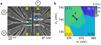
Figure 1: Experimental setup. a, Scanning electron micrograph of a device that is nominally identical to the one used. A double dot is formed under plunger gates $P_{1}$ and $P_{2}$. A sensor dot is formed beneath plunger gate $P_{S}$. Yellow boxes with an “x” in them represent Ohmic contacts to the quantum well. The direction of the external magnetic field $B^{z}$ is indicated. b, Pauli spin blockade at the (3,1)-(4,0) charge transition. The trapezoid in the (4,0) charge region indicates the Pauli spin blockade region. $S$ is the measured charge-sensor signal. The detuning $\epsilon$ is defined as a change in the plunger gate voltages along the diagonal of the charge stability diagram such that $(\Delta V_{1},\Delta V_{2})=(-\epsilon,\epsilon)$, with $\epsilon=0$ at the (4,0)-(3,1) charge transition.

II Device and Hamiltonian

We employ a double quantum dot fabricated in an undoped Si/SiGe heterostructure with an overlapping-gate architecture Zajac et al. (2015); Angus et al. (2007); Zajac et al. (2015); Borselli et al. (2015); Zajac et al. (2016); Connors et al. (2021) (Fig. 1a). Quantum dots 1 and 2, which together form the double dot, are formed beneath plunger gates $P_{1}$ and $P_{2}$, respectively, with their electron occupancies controlled by the positive voltages applied to the gates, $V_{1}$ and $V_{2}$. We use the quantum dot beneath gate $P_{S}$ as a charge sensor and measure its conductance via rf reflectometry for fast spin-state readout Reilly et al. (2007); Barthel et al. (2009); Connors et al. (2020). The device is cooled in a dilution refrigerator to a base temperature of about 10 mK.

We tune the device to the (4,0)-(3,1) charge transition, where the (i,j) notation indicates that dot 1(2) is occupied with i(j) electrons (Fig. 1b). We describe this system of four electrons using a phenomenological Hubbard model, in addition to valley, spin, and spin-valley terms in the total Hamiltonian: $H=H^{Hub}+H^{v}+H^{s}+H^{sv}$ (see Methods). Within this framework, the relevant four-electron quantum states consist of Slater determinants of the lowest four single-particle energy levels of the two quantum dots: two valleys ($-$ and $+$) in dot 1 and two valleys ($-$ and $+$) in dot 2. In the (4,0) charge configuration, both valleys in dot 1 are full. In the (3,1) charge configuration, two electrons in dot 1 fill a single valley, either $+$ or $-$. The remaining electron occupies the unfilled valley in dot 1, and the electron in dot 2 can occupy either of its valleys. Below, we refer to the unpaired electrons (those without another electron in the same dot and valley) as “valence” electrons, and we label the four-spin states by the configuration of the valence electrons. Figure 2a, for example, depicts the state $\ket{\uparrow^{\scalebox{0.6}{$+$}}\downarrow^{\scalebox{0.6}{$-$}}}$, where the left arrow indicates the spin of the valence electron in dot 1, the right arrow indicates the spin of the valence electron in dot 2, and the superscripts indicate the valley of each spin. As we show in the following, while, in general, the electron dynamics in our device involve all four electrons, viewing these four-electron spin states as effective two-electron states results in a surprisingly intuitive and useful picture of the system.

In the absence of spin-valley coupling, the low-energy states of this Hamiltonian yield an effective singlet-triplet qubit Hu and Das Sarma (2001); Barnes et al. (2011); Vorojtsov et al. (2004); Nielsen et al. (2013); Harvey-Collard et al. (2017, 2018); West et al. (2019); Connors et al. (2021); Jock et al. (2021); Seedhouse et al. (2021); Liu et al. (2021), whose eigenstates are $\ket{S^{\scalebox{0.6}{$+$}\scalebox{0.6}{$-$}}}=(\ket{\uparrow^{\scalebox{0.6}{$+$}}\downarrow^{\scalebox{0.6}{$-$}}}-\ket{\downarrow^{\scalebox{0.6}{$+$}}\uparrow^{\scalebox{0.6}{$-$}}})/\sqrt{2}$ and $\ket{T_{0}^{\scalebox{0.6}{$+$}\scalebox{0.6}{$-$}}}=(\ket{\uparrow^{\scalebox{0.6}{$+$}}\downarrow^{\scalebox{0.6}{$-$}}}+\ket{\downarrow^{\scalebox{0.6}{$+$}}\uparrow^{\scalebox{0.6}{$-$}}})/\sqrt{2}$. These states are separated in energy by the exchange coupling $J(\epsilon)$. In addition, if $J(\epsilon)<\Delta E_{Z}=g_{1}\mu_{B}B^{z}-g_{2}\mu_{B}B^{z}$, where $g_{1(2)}$ is the $g$ factor of dot 1(2) Liu et al. (2021); Connors et al. (2021) and $B^{z}$ is the externally applied in-plane magnetic field, the eigenstates of the singlet-triplet qubit are $(\ket{T_{0}^{\scalebox{0.6}{$+$}\scalebox{0.6}{$-$}}}+\ket{S^{\scalebox{0.6}{$+$}\scalebox{0.6}{$-$}}})/\sqrt{2}=\ket{\uparrow^{\scalebox{0.6}{$+$}}\downarrow^{\scalebox{0.6}{$-$}}}$ and $(\ket{T_{0}^{\scalebox{0.6}{$+$}\scalebox{0.6}{$-$}}}-\ket{S^{\scalebox{0.6}{$+$}\scalebox{0.6}{$-$}}})/\sqrt{2}=\ket{\downarrow^{\scalebox{0.6}{$+$}}\uparrow^{\scalebox{0.6}{$-$}}}$ Petta et al. (2005); Foletti et al. (2009).

All measurements presented in this paper begin with the state initialized as a singlet in the (4,0) charge configuration. We separate the valence electrons into the $\ket{S^{\scalebox{0.6}{$+$}\scalebox{0.6}{$-$}}}$ state by tunneling into the (3,1) configuration. Then, we manipulate the joint spin state of the valence electrons by pulsing $\epsilon$ (Fig. 1b). We define $\epsilon$ such that positive values of $\epsilon$ feature positive voltage pulses away from the idling tuning on $P_{2}$ and negative voltage pulses on $P_{1}$. To measure the device, we perform a Pauli spin blockade (PSB) readout Petta et al. (2005); Foletti et al. (2009), which allows us to distinguish between the singlet and triplet configurations of the two valence electrons (Fig. 1b). In the absence of interactions with other spin states, such as any of the polarized triplets, the two electrons remain with high probability in the subspace spanned by $\ket{S^{\scalebox{0.6}{$+$}\scalebox{0.6}{$-$}}}$ and $\ket{T_{0}^{\scalebox{0.6}{$+$}\scalebox{0.6}{$-$}}}$.

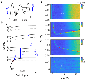
Figure 2: Spin funnels. a, Schematic of occupied levels associated with the $\ket{\uparrow^{\scalebox{0.6}{$+$}}\downarrow^{\scalebox{0.6}{$-$}}}$ state. b, Energy level diagram showing the relevant energy levels for the spin funel experiments. $E_{Z}=\bar{g}\mu_{B}B^{z}$ is the average Zeeman energy of the two dots. The red circle denotes the mixing point between $\ket{S^{\scalebox{0.6}{$+$}\scalebox{0.6}{$-$}}}$ and $\ket{T_{-}^{\scalebox{0.6}{$+$}\scalebox{0.6}{$-$}}}$. c, The four spin funnels observed in this experiment. In each graph the valley configuration of the relevant $T_{-}$ state is indicated. The dashed red lines for the second and third spin funnels show the extracted values used to calculate $E^{v}_{1(2)}$. $\Delta S$ is the measured charge-sensor signal minus the most likely signal value occurring at $\epsilon<5$ mV (corresponding to the singlet signal value) in each plot.

III Valley splittings

We begin by extracting the valley splitting in each dot, $E^{v}_{1(2)}$, from a “spin funnel” measurement Petta et al. (2005); Liu et al. (2021). Near zero magnetic field, a spin funnel reveals the field $B^{z}$ where the lowest-energy singlet, $\ket{S^{\scalebox{0.6}{$+$}\scalebox{0.6}{$-$}}}$, and the lowest-energy polarized triplet, $\ket{T_{-}^{\scalebox{0.6}{$+$}\scalebox{0.6}{$-$}}}=\ket{\downarrow^{\scalebox{0.6}{$+$}}\downarrow^{\scalebox{0.6}{$-$}}}$, come into resonance, which occurs when $\bar{g}\mu_{B}B^{z}=J(\epsilon)$, where $\bar{g}=(g_{1}+g_{2})/2$ is the average $g$-factor of dots 1 and 2 (Fig. 2b). However, at higher magnetic fields, the excited $T_{-}$ states ($\ket{T_{-}^{\scalebox{0.6}{$-$}\scalebox{0.6}{$-$}}}=\ket{\downarrow^{\scalebox{0.6}{$-$}}\downarrow^{\scalebox{0.6}{$-$}}}$, $\ket{T_{-}^{\scalebox{0.6}{$+$}\scalebox{0.6}{$+$}}}=\ket{\downarrow^{\scalebox{0.6}{$+$}}\downarrow^{\scalebox{0.6}{$+$}}}$, or $\ket{T_{-}^{\scalebox{0.6}{$-$}\scalebox{0.6}{$+$}}}=\ket{\downarrow^{\scalebox{0.6}{$-$}}\downarrow^{\scalebox{0.6}{$+$}}}$) come into resonance with $\ket{S^{\scalebox{0.6}{$+$}\scalebox{0.6}{$-$}}}$ when $\bar{g}\mu_{B}B^{z}=\Delta+J(\epsilon)$, where $\Delta$ can be any of $\{E^{v}_{1},E^{v}_{2},E^{v}_{1}+E^{v}_{2}\}$ (Fig. 2b).

Figure 2c shows the four spin funnels we observe, which in the following we refer to as the “first,” “second,” “third,” and “fourth” spin funnels according to the order in which they occur when sweeping the magnetic field from zero. In each panel, the thin bright lines indicate the magnetic-field and detuning values with relatively high triplet-return probabilities, which occur when $\ket{S^{\scalebox{0.6}{$+$}\scalebox{0.6}{$-$}}}$ comes into resonance with one of the above mentioned triplet states. We determine $J(\epsilon)$ from the first spin funnel, together with measurements of coherent exchange oscillations (see Methods). We use the magnetic-field and detuning values of the second and third spin funnels to extract the valley splitting of dot 1 and dot 2, respectively.

The data of Fig. 2c reveal two notable features. First, $E^{v}_{1}$ and $E^{v}_{2}$ clearly depend on the gate voltages, as evidenced by the downward and upward sloping lines of the second and third spin funnels at large values of $\epsilon$. We extract the voltage dependencies of the valley splitting of each dot by assuming that $E^{v}_{1}=E^{v}_{1}(\Delta V_{1})$ and $E^{v}_{2}=E^{v}_{2}(\Delta V_{2})$. We find $dE^{v}_{1}/d\Delta V_{1}=0.066$ meV/V and $dE^{v}_{2}/d\Delta V_{2}$ varies from $0.033$ to $0.54$ meV/V across the voltage range that we measure. The negative slope of the second spin funnel occurs because positive changes to $\epsilon$ involve a negative change to $\Delta V_{1}$. These values are in agreement with recent reports in Si quantum dots Liu et al. (2021); Jock et al. (2021).

The second notable feature of the data in Fig. 2c is the second and third spin funnels are substantially brighter than the first, especially deep in (3,1). Usually, the dominant $S$-$T_{-}$ mixing mechanism is a transverse hyperfine gradient Stepanenko et al. (2012), which is expected to be small in Si. The presence of a small transverse gradient, for example, explains why the first spin funnel is relatively dim. To understand the prominence of the second and third spin funnels, recall that deep in the (3,1), where $J(\epsilon)\approx 0$, the singlet-triplet-qubit eigenstates are $\ket{\uparrow^{\scalebox{0.6}{$+$}}\downarrow^{\scalebox{0.6}{$-$}}}$ and $\ket{\downarrow^{\scalebox{0.6}{$+$}}\uparrow^{\scalebox{0.6}{$-$}}}$. On the second spin funnel, the state $\ket{\downarrow^{\scalebox{0.6}{$-$}}\downarrow^{\scalebox{0.6}{$-$}}}$ comes into resonance with these two eigenstates. A mechanism that simultaneously flips the spin in dot 1 and changes its valley could induce a rapid transition between the triplet and one of the eigenstates. Likewise, a mechanism that can simultaneously flip the spin and change the valley of the electron in dot 2 could generate a similar strong transition between $\ket{\downarrow^{\scalebox{0.6}{$+$}}\downarrow^{\scalebox{0.6}{$+$}}}$ and the opposite eigenstate.

IV Single-Spin-valley coupling

In Si, spin-orbit coupling can generate such a “spin-valley” coupling between single-spin states with different spin and valley quantum numbers: $\braket{\uparrow^{\scalebox{0.6}{$-$}}}{H^{sv}}{\downarrow^{\scalebox{0.6}{$+$}}}=\Delta^{sv}$ Yang et al. (2013); Hao et al. (2014); Huang and Hu (2014); Zhang et al. (2020). Spin-valley couplings have been explored for their effects on spin-state energies Hao et al. (2014); Scarlino et al. (2017); Veldhorst et al. (2015), spin relaxation times Yang et al. (2013); Tahan and Joynt (2014); Zhang et al. (2020); Hollmann et al. (2020), and as ways to assist with qubit manipulation Corna et al. (2018); Bourdet et al. (2018); Jock et al. (2021). However, despite the prominent $S$-$T_{-}$ mixing observed here and previously Liu et al. (2021), which suggests substantial spin-valley coupling rates, this mechanism has not been explored as a method itself to coherently manipulate spin states.

To investigate this possibility, we set $B^{z}=279.2$ mT, near the second spin funnel. We prepare the state $\ket{\uparrow^{\scalebox{0.6}{$+$}}\downarrow^{\scalebox{0.6}{$-$}}}$ in the (3,1) charge configuration by adiabatic separation of the $\ket{T_{0}^{\scalebox{0.6}{$+$}\scalebox{0.6}{$-$}}}$ state in the presence of a $g$-factor difference (see Methods), and then we pulse to different values of $\epsilon$ deep in (3,1). Near $\epsilon=30$ mV, where $J(\epsilon)\approx 0$, we observe prominent Rabi oscillations with frequency $f_{1}=8.2$ MHz. These oscillations occur because the excited triplet $\ket{\downarrow^{\scalebox{0.6}{$-$}}\downarrow^{\scalebox{0.6}{$-$}}}$ comes into resonance with the $\ket{\uparrow^{\scalebox{0.6}{$+$}}\downarrow^{\scalebox{0.6}{$-$}}}$ state (Figs. 3a-b). The oscillation frequency is determined by the single-spin-valley coupling in dot 1, such that $f_{1}=2\braket{\uparrow^{\scalebox{0.6}{$+$}}\downarrow^{\scalebox{0.6}{$-$}}}{H^{sv}}{\downarrow^{\scalebox{0.6}{$-$}}\downarrow^{\scalebox{0.6}{$-$}}}=2\Delta^{sv}_{1}$, where we have set Planck’s constant $h=1$. While this is apparent within the two-electron picture, it is indeed also true in the full four-electron picture (see Methods). When we instead prepare the state $\ket{\downarrow^{\scalebox{0.6}{$+$}}\uparrow^{\scalebox{0.6}{$-$}}}$ (by adiabatic separation of the $\ket{S^{\scalebox{0.6}{$+$}\scalebox{0.6}{$-$}}}$ state) at the same magnetic field, we observe no Rabi oscillations (Fig. 3c), which is expected since $\braket{\downarrow^{\scalebox{0.6}{$+$}}\uparrow^{\scalebox{0.6}{$-$}}}{H^{sv}}{\downarrow^{\scalebox{0.6}{$-$}}\downarrow^{\scalebox{0.6}{$-$}}}=0$. Such a transition would require a pure spin flip in dot 2 and a pure valley change in dot 1.

Furthermore, when we prepare $\ket{\downarrow^{\scalebox{0.6}{$+$}}\uparrow^{\scalebox{0.6}{$-$}}}$ at $B^{z}=380.8$ mT, near the third spin funnel, we observe prominent Rabi oscillations with $f_{2}=2\braket{\downarrow^{\scalebox{0.6}{$+$}}\uparrow^{\scalebox{0.6}{$-$}}}{H^{sv}}{\downarrow^{\scalebox{0.6}{$+$}}\downarrow^{\scalebox{0.6}{$+$}}}=2\Delta^{sv}_{2}=15.2$ MHz, but we do not observe Rabi oscillations when we prepare $\ket{\uparrow^{\scalebox{0.6}{$+$}}\downarrow^{\scalebox{0.6}{$-$}}}$ (Figs. 3d-f). Tuning the magnetic field away from either the second or third spin funnel and performing the same experiment yield no measurable oscillations with either initial state (see Methods). We hypothesize that the features visible in Figs. 3c and 3e result from spurious coupling between the states $\ket{\downarrow^{\scalebox{0.6}{$+$}}\uparrow^{\scalebox{0.6}{$-$}}}$ and $\ket{\uparrow^{\scalebox{0.6}{$+$}}\downarrow^{\scalebox{0.6}{$-$}}}$, likely due to residual exchange coupling (see Methods).

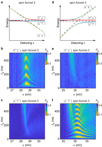
Figure 3: Single-spin Rabi oscillations driven by spin-valley coupling. a, Energy level diagram at large $\epsilon$ and with $B^{z}$ near the second spin funnel. Here, the excited triplet state $\ket{\downarrow^{\scalebox{0.6}{$-$}}\downarrow^{\scalebox{0.6}{$-$}}}$ (green) hybridizes with the product state $\ket{\uparrow^{\scalebox{0.6}{$+$}}\downarrow^{\scalebox{0.6}{$-$}}}$ (red). The black dashed lines show the case in the absence of spin-valley coupling for comparison. b, Spin-valley-driven Rabi oscillations between $\ket{\uparrow^{\scalebox{0.6}{$+$}}\downarrow^{\scalebox{0.6}{$-$}}}$ and $\ket{\downarrow^{\scalebox{0.6}{$-$}}\downarrow^{\scalebox{0.6}{$-$}}}$, acquired at $B^{z}=279.2$ mT, near the second spin funnel. We initialize and readout the state $\ket{\uparrow^{\scalebox{0.6}{$+$}}\downarrow^{\scalebox{0.6}{$-$}}}$ before and after the evolution for a variable time $t_{e}$ and at variable $\epsilon$. c, Control experiment corresponding to b where we prepare and readout the state $\ket{\downarrow^{\scalebox{0.6}{$+$}}\uparrow^{\scalebox{0.6}{$-$}}}$. No Rabi oscillations are visible. d, Energy level diagram at large $\epsilon$ and with $B^{z}$ near the third spin funnel. Here, the excited triplet state $\ket{\downarrow^{\scalebox{0.6}{$+$}}\downarrow^{\scalebox{0.6}{$+$}}}$ (green) hybridizes with $\ket{\downarrow^{\scalebox{0.6}{$+$}}\uparrow^{\scalebox{0.6}{$-$}}}$ (blue). e, f, Same measurements as in b and c, respectively, but conducted with $B^{z}=380.8$ mT, near the third spin funnel. Here, spin-valley-driven Rabi oscillations between $\ket{\downarrow^{\scalebox{0.6}{$+$}}\uparrow^{\scalebox{0.6}{$-$}}}$ and $\ket{\downarrow^{\scalebox{0.6}{$+$}}\downarrow^{\scalebox{0.6}{$+$}}}$ are visible, but not between $\ket{\uparrow^{\scalebox{0.6}{$+$}}\downarrow^{\scalebox{0.6}{$-$}}}$ and $\ket{\downarrow^{\scalebox{0.6}{$+$}}\downarrow^{\scalebox{0.6}{$+$}}}$.

We interpret the data of Fig. 3 as evidence for combined spin-valley Rabi oscillations between effective single-electron states. Specifically, Fig. 3b corresponds to simultaneous spin flips and valley changes in dot 1, and Fig. 3f corresponds to simultaneous spin flips and valley changes in dot 2. Because the spin-valley coupling is an “always-on” matrix element, no ac magnetic or electric fields are required for these spin rotations. Thus, spin-valley coupling offers a method for single-spin control which complements traditional methods based on oscillating fields. In the present context, these single-spin oscillations are facilitated by singlet-triplet initialization and readout. Note that the quantum states, which we label as effective two-electron states with the valence configuration, are actually four-electron states. Thus, within the two-electron picture, the data of Fig. 3 represent a single spin undergoing spin and valley oscillations. Within the four-electron picture, however, all of the electrons in a particular dot will participate in the spin-valley oscillations. In Fig. 3b, for example, all three electrons undergo collective spin-valley changes (see Methods). Nevertheless, the two-electron picture provides an intuitive picture of our four-electron system and accurately predicts the spin-valley couplings we observe.

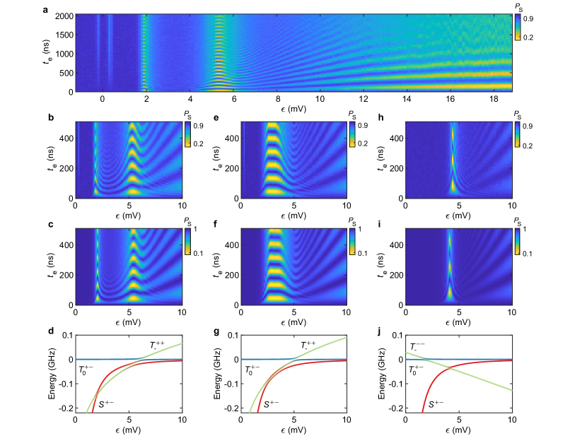
Figure 4: $S$-$T_{-}$ oscillations driven by spin-valley coupling. a, With $B^{z}=372.3$ mT, near the third spin funnel, we prepare the state $\ket{S^{\scalebox{0.6}{$+$}\scalebox{0.6}{$-$}}}$ and pulse to different values of $\epsilon$ for different evolution times $t_{e}$. The first two vertical lines in the data between $\epsilon=-1$ mV and 1 mV result from the first and second spin funnels. The two sets of Rabi oscillations near $\epsilon=2$ mV and 5 mV are $S$-$T_{-}$ Rabi oscillations. The oscillations for $\epsilon>6$ mV are exchange- and gradient-driven $S$-$T_{0}$ oscillations. b, High-resolution scan of the two sets of Rabi oscillations at $B^{z}=372.3$ mT. c, Numerical simulation corresponding to b. d, Numerically computed energies for the three relevant levels in c. e, High-resolution scan of Rabi oscillations at $B^{z}=371.3$ mT, when the two $S$-$T_{-}$ avoided crossings have merged. f, Numerical simulation corresponding to e. g, Numerically computed energies for the three relevant levels in f. h, High-resolution scan of Rabi oscillations at $B^{z}=295.0$ mT, on the second spin funnel. i, Numerical simulation corresponding to h. j, Numerically computed energies for the three relevant levels in i.

V Singlet-triplet and triplet-triplet spin-valley coupling

Given the existence of single-spin-valley matrix elements associated with dots 1 and 2 ($\Delta^{sv}_{1}$ and $\Delta^{sv}_{2}$, respectively), we also expect that strong singlet-triplet mixing should occur when $J(\epsilon)$ is appreciable, and when the singlet-triplet qubit eigenstates are effective singlets and triplets, instead of effective product states. Indeed, one can see that $\braket{S^{\scalebox{0.6}{$+$}\scalebox{0.6}{$-$}}}{H^{sv}}{T_{-}^{\scalebox{0.6}{$-$}\scalebox{0.6}{$-$}}}=\Delta^{sv}_{1}/\sqrt{2}$, and $\braket{S^{\scalebox{0.6}{$+$}\scalebox{0.6}{$-$}}}{H^{sv}}{T_{-}^{\scalebox{0.6}{$+$}\scalebox{0.6}{$+$}}}=-\Delta^{sv}_{2}/\sqrt{2}$ (see Methods).

To test for this effect, we set $B^{z}=372.3$ mT, still near the third spin funnel. At this field, the $\ket{S^{\scalebox{0.6}{$+$}\scalebox{0.6}{$-$}}}$ and $\ket{T_{-}^{\scalebox{0.6}{$+$}\scalebox{0.6}{$+$}}}$ states come into resonance when $J(\epsilon)\gg\Delta E_{Z}$. We initialize $\ket{S^{\scalebox{0.6}{$+$}\scalebox{0.6}{$-$}}}$ and pulse $\epsilon$ suddenly, which preserves the singlet state as the charge configuration changes. After variable evolution time, we pulse $\epsilon$ to the PSB region for readout. Against a broad background of exchange-driven and gradient-driven $S$-$T_{0}$ oscillations, two narrow regions with pronounced and long-lived Rabi oscillations are visible (Fig. 4a).

A high resolution scan of the two avoided crossings (Fig. 4b) agrees strikingly well with numerical simulations (see Methods) (Fig. 4c). Figure 4d shows the energies of the relevant three states in these simulations. Because $E^{v}_{2}(\Delta V_{2})$ increases with $\epsilon$, the energy the of $\ket{T_{-}^{\scalebox{0.6}{$+$}\scalebox{0.6}{$+$}}}$ state intersects that of the $\ket{S^{\scalebox{0.6}{$+$}\scalebox{0.6}{$-$}}}$ state twice at this magnetic field, yielding two different avoided crossings between these states. In either case, the Rabi frequency is $f_{2}^{ST}=11.3$ MHz. Note that $f_{2}^{ST}/f_{2}=0.74$, in agreement with our expectation that $\braket{S^{\scalebox{0.6}{$+$}\scalebox{0.6}{$-$}}}{H^{sv}}{T_{-}^{\scalebox{0.6}{$+$}\scalebox{0.6}{$+$}}}=-\Delta^{sv}_{2}/\sqrt{2}$

At a slightly lower magnetic field $B^{z}=371.3$ mT, the two $S$-$T_{-}$ avoided crossings merge, yielding an extended avoided crossing with pronounced Rabi oscillations of the same frequency (Fig. 4e). As above, numerical simulations (Figs. 4f-g) agree with our data. When we set $B^{z}=295.0$ mT, on the second spin funnel, we only observe one avoided crossing (Fig. 4h) because $E^{v}_{1}(\Delta V_{1})$ decreases with $\epsilon$ and therefore the energy of the $\ket{T_{-}^{\scalebox{0.6}{$-$}\scalebox{0.6}{$-$}}}$ state only intersects that of the $\ket{S^{\scalebox{0.6}{$+$}\scalebox{0.6}{$-$}}}$ state once (Fig. 4j). The oscillation frequency $f_{1}^{ST}=6$ MHz and $f_{1}^{ST}/f_{1}=0.73$, again in agreement with the expectation that $\braket{S^{\scalebox{0.6}{$+$}\scalebox{0.6}{$-$}}}{H^{sv}}{T_{-}^{\scalebox{0.6}{$-$}\scalebox{0.6}{$-$}}}=\Delta^{sv}_{1}/\sqrt{2}$.

These data represent evidence of $S$-$T_{-}$ Rabi oscillations, driven by spin-valley coupling. Previously, $S$-$T_{-}$ Rabi oscillations in Si (or $S$-$T_{+}$ oscillations in GaAs quantum dots) have not been observed, because the most common mechanisms for $S$-$T_{-}$ mixing occur in parameter regimes that feature extreme sensitivity to hyperfine or charge noise and significant decoherence Stepanenko et al. (2012); Petta et al. (2010); Nichol et al. (2015). Despite this obstacle, however, coherent oscillations of $S$-$T_{-}$ superposition states in Si (or $S$-$T_{+}$ states in GaAs) have been observed through Landau-Zener interferometry Petta et al. (2010); Wu et al. (2014); Fogarty et al. (2018). Our results, however, show how the spin-valley coupling overcomes the longstanding challenge of manipulating $S$-$T_{-}$ systems and enables straightforward, universal quantum control of an $S$-$T_{-}$ qubit.

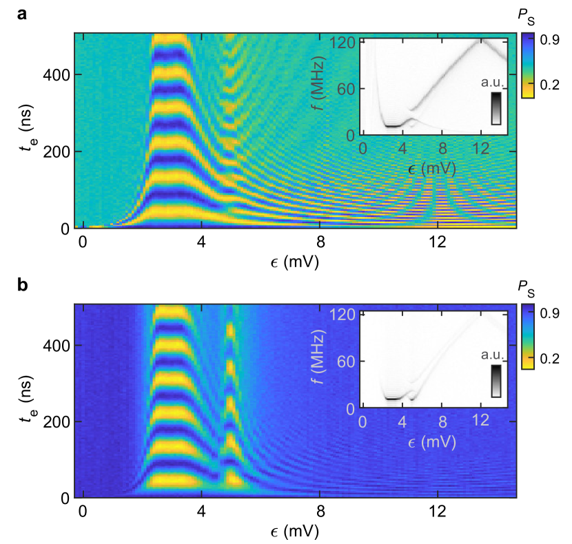
Figure 5: Coherent manipulation of joint spin states through spin-valley coupling. a, Ramsey oscillations at different values of $\epsilon$. Inset: Absolute value of the fast Fourier transform of the data. b, Oscillations measured with a $\pi$ pulse at $\epsilon=3$ mV before and after the evolution. The $\pi$ pulses map $\ket{S^{\scalebox{0.6}{$+$}\scalebox{0.6}{$-$}}}$ to $\ket{T_{-}^{\scalebox{0.6}{$+$}\scalebox{0.6}{$+$}}}$ and vice versa. The oscillations near $\epsilon=5$ mV correspond to $T_{0}$-$T_{-}$ Rabi oscillations, also mediated by spin-valley coupling. Inset: Absolute value of the fast Fourier transform of the data.

To illustrate the potential of spin-valley coupling for full quantum control of $S$-$T_{-}$ states, we set $B^{z}=371.1$ mT, where the two $S$-$T_{-}$ avoided crossings on the third spin funnel merge. We perform a Ramsey experiment by applying a $3\pi/2$ pulse at the avoided crossing before an evolution segment of variable time and $\epsilon$, and a $\pi/2$ pulse after the evolution (Fig. 5a). Now, at values of $\epsilon>6$ mV, we observe relatively high-frequency oscillations corresponding to the time evolution of $S$-$T_{-}$ superposition states. In this range, the frequency of these oscillations increases with $\epsilon$ because of the $\epsilon$ dependence of $E^{v}_{2}$ which determines the energy of the $\ket{T_{-}^{\scalebox{0.6}{$+$}\scalebox{0.6}{$+$}}}$ state (Fig. 5g). Because of the approximately linear increase of $E^{v}_{2}(\Delta V_{2})$ with $\epsilon$, the coherence of these oscillations is nearly constant. Such a scenario, where the coherence of an electrically-controlled multi-electron spin qubit does not decrease with frequency, is rare because such qubit splittings are usually highly non-linear functions of voltages Petta et al. (2005); Dial et al. (2013). We discuss the coherence of these oscillations in further detail below. More complicated pulse sequences are straightforward to implement. In Methods, we discuss a spin-echo experiment, which improves the coherence time of $S$-$T_{-}$ superposition states by roughly a factor of 10.

A close inspection of Fig. 5a reveals an additional set of oscillations near $\epsilon=5$ mV. To elucidate these oscillations, we prepare the $\ket{T_{-}^{\scalebox{0.6}{$+$}\scalebox{0.6}{$+$}}}$ state by applying a $\pi$ pulse at the $S$-$T_{-}$ avoided crossing before pulsing to different values of $\epsilon$ (Fig. 5b). After a variable evolution time, we apply another $\pi$ pulse on resonance, effectively mapping $\ket{T_{-}^{\scalebox{0.6}{$+$}\scalebox{0.6}{$+$}}}$ back to $\ket{S^{\scalebox{0.6}{$+$}\scalebox{0.6}{$-$}}}$. The data from this experiment reveal another avoided crossing near $\epsilon=5$ mV, which we attribute to mixing between $\ket{T_{-}^{\scalebox{0.6}{$+$}\scalebox{0.6}{$+$}}}$ and $\ket{T_{0}^{\scalebox{0.6}{$+$}\scalebox{0.6}{$-$}}}$ (Fig. 5g). These triplet-triplet oscillations have a similar frequency as the main avoided crossing, because $\braket{T_{0}^{\scalebox{0.6}{$+$}\scalebox{0.6}{$-$}}}{H^{sv}}{T_{-}^{\scalebox{0.6}{$+$}\scalebox{0.6}{$+$}}}=\Delta^{sv}_{2}/\sqrt{2}$ (and $\braket{T_{0}^{\scalebox{0.6}{$+$}\scalebox{0.6}{$-$}}}{H^{sv}}{T_{-}^{\scalebox{0.6}{$-$}\scalebox{0.6}{$-$}}}=\Delta^{sv}_{1}/\sqrt{2}$). Such triplet-triplet oscillations represent a previously-unexplored spin-state transition driven by spin-valley coupling between effective joint spin states in a double quantum dot.

As a final confirmation that these effects originate from spin-orbit coupling, we measure the dependence of $\Delta^{sv}_{1}$ and $\Delta^{sv}_{2}$ on the direction of the external in-plane magnetic field (see Methods). We find that the magnitudes of both spin-valley couplings oscillate with the in-plane field angle as expected for spin-orbit coupling (see Methods). In addition to corroborating the notion that the spin-valley coupling in our system originates from spin-orbit coupling, these data reveal differences in the relative strengths of the Rashba and Dresselhaus spin-orbit couplings and valley phase differences between quantum dots Zhang et al. (2020).

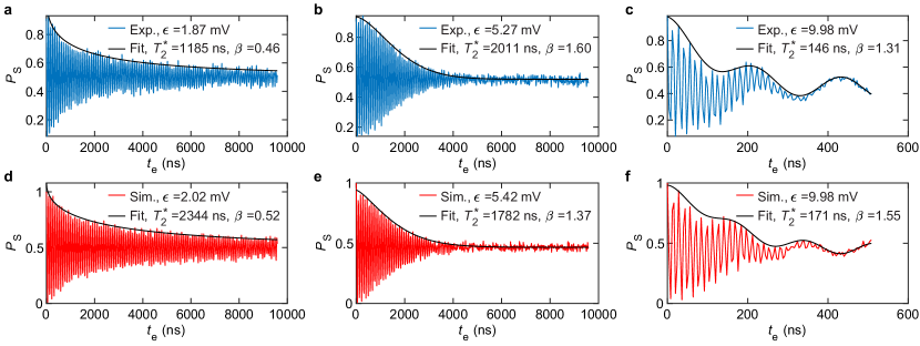
Figure 6: Measured and simulated $S$-$T_{-}$ oscillations on the third spin funnel, where the two avoided crossings are separate. a, Measured Rabi oscillations at the left avoided crossing. The data are fit to an equation of the form $P_{S}(t)=P_{0}+A\cos(\omega t+\phi)\exp\left[-(t/T_{2}^{*})^{\beta}\right]$, with $P_{0}$, $A$, $\omega$, $\phi$, $T_{2}^{*}$, and $\beta$ as fit parameters. The overlaid black line is $P_{0}+A\exp\left[-(t/T_{2}^{*})^{\beta}\right]$. b, Measured Rabi oscillations at the right avoided crossing. c, Measured Ramsey oscillations near $\epsilon=10$ mV. The slow background oscillations are $S$-$T_{0}$ oscillations. We fit the data to an equation of the form $P_{S}(t)=P_{0}+A\cos(\omega t+\phi)\exp\left[-(t/T_{2}^{*})^{\beta}\right]+A_{2}\cos(\omega_{2}t+\phi_{2})$, where $A_{2}$, $\omega_{2}$, and $\phi_{2}$ describe the $S$-$T_{0}$ oscillations. The black line is $P_{0}+A\exp\left[-(t/T_{2}^{*})^{\beta}\right]+A_{2}\cos(\omega_{2}t+\phi)$. d, Numerical simulations corresponding to panel a and fit. We choose the value of $\epsilon$ corresponding to the local minimum in the oscillation frequency in the region near $\epsilon=2$ mV, corresponding to the location of the left avoided crossing. e, Numerical simulation corresponding to b and fit. We choose the value of $\epsilon$ corresponding to the local minimum in the oscillation frequency in the region near $\epsilon=5$ mV, corresponding to the location of the right avoided crossing. f, Numerical simulation corresponding to c. Here we chose the same value of $\epsilon$ as in c. In all cases, the measured and simulated values of $T_{2}^{*}$ and $\beta$ show reasonably good agreement with each other.

VI Spin-valley oscillation coherence

Finally, we analyze the coherence of the observed spin-valley $S$-$T_{-}$ oscillations. We set $B^{z}=370.4$ mT, on the third spin funnel, where the two avoided crossings remain separate, and perform Ramsey experiments using a similar procedure to that described above. Figures 6a-c show the time series obtained from these experiments at three specific detunings: the two values of $\epsilon$ where the $S$-$T_{-}$ avoided crossings occur, and one value of $\epsilon$ deep in (3,1). Both avoided crossings feature long-lived coherence (Fig. 6a-b), with Rabi oscillations persisting for at least several microseconds.

The decay of Rabi oscillations at both avoided crossings is clearly non-Gaussian (Figs. 6a-b), especially at the left avoided crossing. We attribute this fact to the non-Gaussian nature of fluctuations in the energy splitting at the avoided crossing Makhlin and Shnirman (2004). For the left avoided crossing, we expect this effect to be pronounced, because the energy splitting in the vicinity of the avoided crossing depends strongly and non-linearly on $\epsilon$. In both cases, however, our numerical simulations (Figs. 6d-e) (see Methods) reproduce both the observed coherence times and decay shapes. The simulations are based on solving the Schrödinger equation for the time evolution of the relevant three levels ($\ket{S^{\scalebox{0.6}{$+$}\scalebox{0.6}{$-$}}}$, $\ket{T_{0}^{\scalebox{0.6}{$+$}\scalebox{0.6}{$-$}}}$, and either $\ket{T_{-}^{\scalebox{0.6}{$-$}\scalebox{0.6}{$-$}}}$ or $\ket{T_{-}^{\scalebox{0.6}{$+$}\scalebox{0.6}{$+$}}}$) and include independent, random, quasistatic magnetic-field fluctuations for each electron (with rms value $\sigma_{B}=8$ $\mu$T, corresponding to an inhomogeneuosly broadened single-spin coherence time of 1 $\mu$s), as well as independent gate-voltage fluctuations on each plunger gate (with rms values 34 $\mu$V and 92 $\mu$V for $P_{1}$ and $P_{2}$, respectively, see Methods).

At $\epsilon=10$ mV, where the oscillations reflect the time evolution of $S$-$T_{-}$ superposition states (in addition to the slower, $S$-$T_{0}$ dynamics), the decay occurs over a timescale of about a hundred nanoseconds (Fig. 6c). Because we assume that the valley splitting $E^{v}_{2}(\Delta V_{2})$ depends only on $V_{2}$, we attribute this decay to electrical noise associated with $V_{2}$. Because of this, and because a similar data set on the second spin funnel reflects the noise associated with $V_{1}$, we can determine the effective gate voltage fluctuations separately for each dot. As above, our numerical simulations reproduce the approximate decay time and shape (Figs. 6f). In the future, this ability to independently resolve electrical fluctuations on separate quantum dots will complement measurements of charge noise based on exchange coupling Dial et al. (2013); Connors et al. (2021); Jock et al. (2021), which depends on the difference between chemical potentials of two dots.

We have performed similar analyses for the second spin funnel and for the third spin funnel at a magnetic field where the avoided crossings have merged (see Methods). In all cases, we achieve roughly the same level of agreement between experiment and simulation, suggesting that our simple three-level model with independent quasi-static electrical and magnetic noise associated with each dot successfully explains the features we observe.

VII Conclusion

We have demonstrated that spin-valley coupling, a phenomenon usually considered a hindrance in Si spin-qubit systems, can enable coherent manipulation of both single- and multi-spin states in Si quantum dots. Our measurements reveal a simple method to control effective single-spin states without ac magnetic or electric fields, as well as $S$-$T_{-}$ Rabi and Ramsey oscillations and previously-unexplored triplet-triplet oscillations. Because of its simplicity, this method of coherent spin manipulation can potentially supplement existing control methods in many existing qubit encodings. Coherent spin manipulation via spin-valley coupling can also immediately add an important capability to charge-noise spectroscopy in Si quantum dots by offering a method to explore local charge noise in quantum-dot spin qubits, complementing standard techniques based on exchange coupling. Finally, our measurements present a striking confirmation of how simple Hubbard models and effective valence-electron pictures can apply to multi-electron systems undergoing complex, collective dynamics.

More broadly, our measurements introduce a new family of spin qubits, including effective single-spin, singlet-triplet, and triplet-triplet qubits based on spin-valley coupling. The long coherence times and ease of control associated with these qubits warrants future work to fully characterize their properties, including gate fidelities. The implementation of systems with multiple spin-valley qubits will likely require that the different spin qubits either have the same valley splittings or different Zeeman energies, which could be potentially achieved through heterostructure engineering Sasaki et al. (2009); Chen et al. (2021b); McJunkin et al. (2021); Neyens et al. (2018), voltage control of valley splittings Yang et al. (2013); Chen et al. (2021b); Hollmann et al. (2020), or local magnetic field control Borjans et al. (2020); Astner et al. (2017). Altogether, these results highlight the suprising usefulness of the valley degree of freedom, a unique feature of electrons in Si, for quantum information processing.

VIII Data Availability

The data that support the findings of this study are available from the corresponding author upon reasonable request.

IX Acknowledgments

We thank Lisa F. Edge of HRL Laboratories, LLC. for the epitaxial growth of the SiGe material. This work was sponsored the Army Research Office under grants W911NF-16-1-0260 and W911NF-19-1-0167. The views and conclusions contained in this document are those of the authors and should not be interpreted as representing the official policies, either expressed or implied, of the Army Research Office or the U.S. Government. The U.S. Government is authorized to reproduce and distribute reprints for Government purposes notwithstanding any copyright notation herein.

X Author Contributions

X.C., E.J.C., and J.M.N. conceptualized the experiment, conducted the investigation, and participated in writing. J.M.N. supervised the effort.

References

- Watson et al. (2018) T. F. Watson, S. G. J. Philips, E. Kawakami, D. R. Ward, P. Scarlino, M. Veldhorst, D. E. Savage, M. G. Lagally, M. Friesen, S. N. Coppersmith, M. A. Eriksson, and L. M. K. Vandersypen, Nature 555, 633 (2018).
- Mi et al. (2018a) X. Mi, M. Benito, S. Putz, D. M. Zajac, J. M. Taylor, G. Burkard, and J. R. Petta, Nature 555, 599 (2018a).
- Xue et al. (2019) X. Xue, T. Watson, J. Helsen, D. Ward, D. Savage, M. Lagally, S. Coppersmith, M. Eriksson, S. Wehner, and L. Vandersypen, Phys. Rev. X 9, 021011 (2019).
- Huang et al. (2019) W. Huang, C. H. Yang, K. W. Chan, T. Tanttu, B. Hensen, R. C. C. Leon, M. A. Fogarty, J. C. C. Hwang, F. E. Hudson, K. M. Itoh, A. Morello, A. Laucht, and A. S. Dzurak, Nature 569, 532 (2019).
- Andrews et al. (2019) R. W. Andrews, C. Jones, M. D. Reed, A. M. Jones, S. D. Ha, M. P. Jura, J. Kerckhoff, M. Levendorf, S. Meenehan, S. T. Merkel, A. Smith, B. Sun, A. J. Weinstein, M. T. Rakher, T. D. Ladd, and M. G. Borselli, Nature Nanotechnology 14, 747 (2019).
- Zwerver et al. (2021) A. M. J. Zwerver, T. Krähenmann, T. F. Watson, L. Lampert, H. C. George, R. Pillarisetty, S. A. Bojarski, P. Amin, S. V. Amitonov, J. M. Boter, R. Caudillo, D. Corras-Serrano, J. P. Dehollain, G. Droulers, E. M. Henry, R. Kotlyar, M. Lodari, F. Luthi, D. J. Michalak, B. K. Mueller, S. Neyens, J. Roberts, N. Samkharadze, G. Zheng, O. K. Zietz, G. Scappucci, M. Veldhorst, L. M. K. Vandersypen, and J. S. Clarke, arXiv:2101.12650 [cond-mat, physics:quant-ph] (2021), arXiv: 2101.12650.
- Noiri et al. (2021) A. Noiri, K. Takeda, T. Nakajima, T. Kobayashi, A. Sammak, G. Scappucci, and S. Tarucha, arXiv preprint arXiv:2108.02626 (2021).
- Xue et al. (2021) X. Xue, M. Russ, N. Samkharadze, B. Undseth, A. Sammak, G. Scappucci, and L. M. Vandersypen, arXiv preprint arXiv:2107.00628 (2021).
- Ando et al. (1982) T. Ando, A. B. Fowler, and F. Stern, Rev. Mod. Phys. 54, 437 (1982).
- Zwanenburg et al. (2013) F. A. Zwanenburg, A. S. Dzurak, A. Morello, M. Y. Simmons, L. C. L. Hollenberg, G. Klimeck, S. Rogge, S. N. Coppersmith, and M. A. Eriksson, Rev. Mod. Phys. 85, 961 (2013).
- Friesen et al. (2007) M. Friesen, S. Chutia, C. Tahan, and S. N. Coppersmith, Phys. Rev. B 75, 115318 (2007).
- Culcer et al. (2010) D. Culcer, Ł. Cywiński, Q. Li, X. Hu, and S. D. Sarma, Physical Review B 82, 155312 (2010).
- Yang et al. (2013) C. H. Yang, A. Rossi, R. Ruskov, N. S. Lai, F. A. Mohiyaddin, S. Lee, C. Tahan, G. Klimeck, A. Morello, and A. S. Dzurak, Nature Comm. 4, 2069 (2013).
- Hao et al. (2014) X. Hao, R. Ruskov, M. Xiao, C. Tahan, and H. Jiang, Nature Comm. 5, 3860 (2014).
- Huang and Hu (2014) P. Huang and X. Hu, Phys. Rev. B 90, 235315 (2014).
- Zhang et al. (2020) X. Zhang, R.-Z. Hu, H.-O. Li, F.-M. Jing, Y. Zhou, R.-L. Ma, M. Ni, G. Luo, G. Cao, G.-L. Wang, X. Hu, H.-W. Jiang, G.-C. Guo, and G.-P. Guo, Phys. Rev. Lett. 124, 257701 (2020).
- Madzik et al. (2021) M. T. Madzik, S. Asaad, A. Youssry, B. Joecker, K. M. Rudinger, E. Nielsen, K. C. Young, T. J. Proctor, A. D. Baczewski, A. Laucht, et al., arXiv preprint arXiv:2106.03082 (2021).
- Mills et al. (2021) A. Mills, C. Guinn, M. Gullans, A. Sigillito, M. Feldman, E. Nielsen, and J. Petta, arXiv preprint arXiv:2111.11937 (2021).
- Schäffler (1997) F. Schäffler, Semicond. Sci. Technol. 12, 1515 (1997).
- Kawakami et al. (2014) E. Kawakami, P. Scarlino, D. R. Ward, F. R. Braakman, D. E. Savage, M. G. Lagally, M. Friesen, S. N. Coppersmith, M. A. Eriksson, and L. M. K. Vandersypen, Nat Nano 9, 666 (2014).
- Jones et al. (2019) A. Jones, E. Pritchett, E. Chen, T. Keating, R. Andrews, J. Blumoff, L. De Lorenzo, K. Eng, S. Ha, A. Kiselev, S. Meenehan, S. Merkel, J. Wright, L. Edge, R. Ross, M. Rakher, M. Borselli, and A. Hunter, Phys. Rev. Applied 12, 014026 (2019).
- Penthorn et al. (2019) N. E. Penthorn, J. S. Schoenfield, J. D. Rooney, L. F. Edge, and H. Jiang, npj Quantum Information 5, 1 (2019).
- Mi et al. (2018b) X. Mi, S. Kohler, and J. R. Petta, Phys. Rev. B 98, 161404 (2018b).
- Borselli et al. (2011) M. G. Borselli, R. S. Ross, A. A. Kiselev, E. T. Croke, K. S. Holabird, P. W. Deelman, L. D. Warren, I. Alvarado-Rodriguez, I. Milosavljevic, F. C. Ku, W. S. Wong, A. E. Schmitz, M. Sokolich, M. F. Gyure, and A. T. Hunter, Appl. Phys. Lett. 98, 375202 (2011).
- Mi et al. (2017) X. Mi, C. G. Peterfalvi, G. Burkard, and J. R. Petta, Phys. Rev. Lett. 119, 176803 (2017).
- Chen et al. (2021a) E. H. Chen, K. Raach, A. Pan, A. A. Kiselev, E. Acuna, J. Z. Blumoff, T. Brecht, M. D. Choi, W. Ha, D. R. Hulbert, M. P. Jura, T. E. Keating, R. Noah, B. Sun, B. J. Thomas, M. G. Borselli, C. Jackson, M. T. Rakher, and R. S. Ross, Phys. Rev. Applied 15, 044033 (2021a).
- Sasaki et al. (2009) K. Sasaki, R. Masutomi, K. Toyama, K. Sawano, Y. Shiraki, and T. Okamoto, Applied Physics Letters 95, 222109 (2009).
- Chen et al. (2021b) E. H. Chen, K. Raach, A. Pan, A. A. Kiselev, E. Acuna, J. Z. Blumoff, T. Brecht, M. D. Choi, W. Ha, D. R. Hulbert, M. P. Jura, T. E. Keating, R. Noah, B. Sun, B. J. Thomas, M. G. Borselli, C. Jackson, M. T. Rakher, and R. S. Ross, Phys. Rev. Applied 15, 044033 (2021b).
- McJunkin et al. (2021) T. McJunkin, E. R. MacQuarrie, L. Tom, S. F. Neyens, J. P. Dodson, B. Thorgrimsson, J. Corrigan, H. E. Ercan, D. E. Savage, M. G. Lagally, R. Joynt, S. N. Coppersmith, M. Friesen, and M. A. Eriksson, Phys. Rev. B 104, 085406 (2021).
- Neyens et al. (2018) S. F. Neyens, R. H. Foote, B. Thorgrimsson, T. Knapp, T. McJunkin, L. Vandersypen, P. Amin, N. K. Thomas, J. S. Clarke, D. Savage, et al., Applied Physics Letters 112, 243107 (2018).
- Goswami et al. (2007) S. Goswami, K. Slinker, M. Friesen, L. McGuire, J. Truitt, C. Tahan, L. Klein, J. Chu, P. Mooney, D. W. Van Der Weide, et al., Nature Physics 3, 41 (2007).
- Hollmann et al. (2020) A. Hollmann, T. Struck, V. Langrock, A. Schmidbauer, F. Schauer, T. Leonhardt, K. Sawano, H. Riemann, N. V. Abrosimov, D. Bougeard, and L. R. Schreiber, Phys. Rev. Applied 13, 034068 (2020).
- Schoenfield et al. (2017) J. S. Schoenfield, B. M. Freeman, and H. Jiang, Nature communications 8, 1 (2017).
- Koh et al. (2012) T. S. Koh, J. K. Gamble, M. Friesen, M. A. Eriksson, and S. N. Coppersmith, Phys. Rev. Lett. 109, 250503 (2012).
- Zajac et al. (2015) D. M. Zajac, T. M. Hazard, X. Mi, K. Wang, and J. R. Petta, Applied Physics Letters 106, 223507 (2015).
- Angus et al. (2007) S. J. Angus, A. J. Ferguson, A. S. Dzurak, and R. G. Clark, Nano Lett. 7, 2051 (2007).
- Borselli et al. (2015) M. G. Borselli, K. Eng, R. S. Ross, T. M. Hazard, K. S. Holabird, B. Huang, A. A. Kiselev, P. W. Deelman, L. D. Warren, I. Milosavljevic, A. E. Schmitz, M. Sokolich, M. F. Gyure, and A. T. Hunter, Nanotechnol. 26, 375202 (2015).
- Zajac et al. (2016) D. M. Zajac, T. M. Hazard, X. Mi, E. Nielsen, and J. R. Petta, Phys. Rev. Applied 6, 054013 (2016).
- Connors et al. (2021) E. J. Connors, J. Nelson, and J. M. Nichol, “Charge-noise spectroscopy of si/sige quantum dots via dynamically-decoupled exchange oscillations,” (2021), arXiv:2103.02448 .
- Reilly et al. (2007) D. J. Reilly, C. M. Marcus, M. P. Hanson, and A. C. Gossard, Applied Physics Letters 91, 162101 (2007).
- Barthel et al. (2009) C. Barthel, D. J. Reilly, C. M. Marcus, M. P. Hanson, and A. C. Gossard, Phys. Rev. Lett. 103, 160503 (2009).
- Connors et al. (2020) E. J. Connors, J. Nelson, and J. M. Nichol, Phys. Rev. Applied 13, 024019 (2020).
- Hu and Das Sarma (2001) X. Hu and S. Das Sarma, Phys. Rev. A 64, 042312 (2001).
- Barnes et al. (2011) E. Barnes, J. P. Kestner, N. T. T. Nguyen, and S. Das Sarma, Phys. Rev. B 84, 235309 (2011).
- Vorojtsov et al. (2004) S. Vorojtsov, E. R. Mucciolo, and H. U. Baranger, Physical Review B 69, 115329 (2004).
- Nielsen et al. (2013) E. Nielsen, E. Barnes, J. P. Kestner, and S. Das Sarma, Phys. Rev. B 88, 195131 (2013).
- Harvey-Collard et al. (2017) P. Harvey-Collard, N. T. Jacobson, M. Rudolph, J. Dominguez, G. A. Ten Eyck, J. R. Wendt, T. Pluym, J. K. Gamble, M. P. Lilly, M. Pioro-Ladrière, and M. S. Carroll, Nature Communications 8, 1029 (2017).
- Harvey-Collard et al. (2018) P. Harvey-Collard, B. D’Anjou, M. Rudolph, N. T. Jacobson, J. Dominguez, G. A. Ten Eyck, J. R. Wendt, T. Pluym, M. P. Lilly, W. A. Coish, M. Pioro-Ladrière, and M. S. Carroll, Phys. Rev. X 8, 021046 (2018).
- West et al. (2019) A. West, B. Hensen, A. Jouan, T. Tanttu, C.-H. Yang, A. Rossi, M. F. Gonzalez-Zalba, F. Hudson, A. Morello, D. J. Reilly, and A. S. Dzurak, Nature Nanotechnology 14, 437 (2019).
- Jock et al. (2021) R. M. Jock, N. T. Jacobson, M. Rudolph, D. R. Ward, M. S. Carroll, and D. R. Luhman, “A silicon singlet-triplet qubit driven by spin-valley coupling,” (2021), arXiv:2102.12068 .
- Seedhouse et al. (2021) A. E. Seedhouse, T. Tanttu, R. C. Leon, R. Zhao, K. Y. Tan, B. Hensen, F. E. Hudson, K. M. Itoh, J. Yoneda, C. H. Yang, A. Morello, A. Laucht, S. N. Coppersmith, A. Saraiva, and A. S. Dzurak, PRX Quantum 2, 010303 (2021).
- Liu et al. (2021) Y. Y. Liu, L. A. Orona, S. F. Neyens, E. R. MacQuarrie, M. A. Eriksson, and A. Yacoby, Phys. Rev. Applied 16, 024029 (2021).
- Petta et al. (2005) J. R. Petta, A. C. Johnson, J. M. Taylor, E. Laird, A. Yacoby, M. D. Lukin, C. M. Marcus, M. P. Hanson, and A. C. Gossard, Science 309, 2180 (2005).
- Foletti et al. (2009) S. Foletti, H. Bluhm, D. Mahalu, V. Umansky, and A. Yacoby, Nature Phys. 5, 903 (2009).
- Stepanenko et al. (2012) D. Stepanenko, M. S. Rudner, B. I. Halperin, and D. Loss, Physical Review B 85, 075416 (2012).
- Scarlino et al. (2017) P. Scarlino, E. Kawakami, T. Jullien, D. Ward, D. Savage, M. Lagally, M. Friesen, S. Coppersmith, M. Eriksson, and L. Vandersypen, Physical Review B 95, 165429 (2017).
- Veldhorst et al. (2015) M. Veldhorst, R. Ruskov, C. H. Yang, J. C. C. Hwang, F. E. Hudson, M. E. Flatté, C. Tahan, K. M. Itoh, A. Morello, and A. S. Dzurak, Phys. Rev. B 92, 201401 (2015).
- Tahan and Joynt (2014) C. Tahan and R. Joynt, Phys. Rev. B 89, 075302 (2014).
- Corna et al. (2018) A. Corna, L. Bourdet, R. Maurand, A. Crippa, D. Kotekar-Patil, H. Bohuslavskyi, R. Laviéville, L. Hutin, S. Barraud, X. Jehl, M. Vinet, S. De Franceschi, Y.-M. Niquet, and M. Sanquer, npj Quantum Inf 4, 6 (2018).
- Bourdet et al. (2018) L. Bourdet, L. Hutin, B. Bertrand, A. Corna, H. Bohuslavskyi, A. Amisse, A. Crippa, R. Maurand, S. Barraud, M. Urdampilleta, et al., IEEE Transactions on Electron Devices 65, 5151 (2018).
- Petta et al. (2010) J. R. Petta, H. Lu, and A. C. Gossard, Science 327, 669 (2010).
- Nichol et al. (2015) J. M. Nichol, S. P. Harvey, M. D. Shulman, A. Pal, V. Umansky, E. I. Rashba, B. I. Halperin, and A. Yacoby, Nat Commun 6 (2015).
- Wu et al. (2014) X. Wu, D. R. Ward, J. R. Prance, D. Kim, J. K. Gamble, R. T. Mohr, Z. Shi, D. E. Savage, M. G. Lagally, M. Friesen, S. N. Coppersmith, and M. A. Eriksson, Proceedings of the National Academy of Sciences 111, 11938 (2014).
- Fogarty et al. (2018) M. A. Fogarty, K. W. Chan, B. Hensen, W. Huang, T. Tanttu, C. H. Yang, A. Laucht, M. Veldhorst, F. E. Hudson, K. M. Itoh, D. Culcer, T. D. Ladd, A. Morello, and A. S. Dzurak, Nature Communications 9, 4370 (2018).
- Dial et al. (2013) O. E. Dial, M. D. Shulman, S. P. Harvey, H. Bluhm, V. Umansky, and A. Yacoby, Phys. Rev. Lett. 110, 146804 (2013).
- Makhlin and Shnirman (2004) Y. Makhlin and A. Shnirman, Phys. Rev. Lett. 92, 178301 (2004).
- Borjans et al. (2020) F. Borjans, X. G. Croot, X. Mi, M. J. Gullans, and J. R. Petta, Nature 577, 195 (2020).
- Astner et al. (2017) T. Astner, S. Nevlacsil, N. Peterschofsky, A. Angerer, S. Rotter, S. Putz, J. Schmiedmayer, and J. Majer, Physical review letters 118, 140502 (2017).