Learning to Fit Morphable Models

Abstract

Fitting parametric models of human bodies, hands or faces to sparse input signals in an accurate, robust, and fast manner has the promise of significantly improving immersion in AR and VR scenarios. A common first step in systems that tackle these problems is to regress the parameters of the parametric model directly from the input data. This approach is fast, robust, and is a good starting point for an iterative minimization algorithm. The latter searches for the minimum of an energy function, typically composed of a data term and priors that encode our knowledge about the problem’s structure. While this is undoubtedly a very successful recipe, priors are often hand defined heuristics and finding the right balance between the different terms to achieve high quality results is a non-trivial task. Furthermore, converting and optimizing these systems to run in a performant way requires custom implementations that demand significant time investments from both engineers and domain experts. In this work, we build upon recent advances in learned optimization and propose an update rule inspired by the classic Levenberg–Marquardt algorithm. We show the effectiveness of the proposed neural optimizer on three problems, 3D body estimation from a head-mounted device, 3D body estimation from sparse 2D keypoints and face surface estimation from dense 2D landmarks. Our method can easily be applied to new model fitting problems and offers a competitive alternative to well-tuned ’traditional’ model fitting pipelines, both in terms of accuracy and speed.

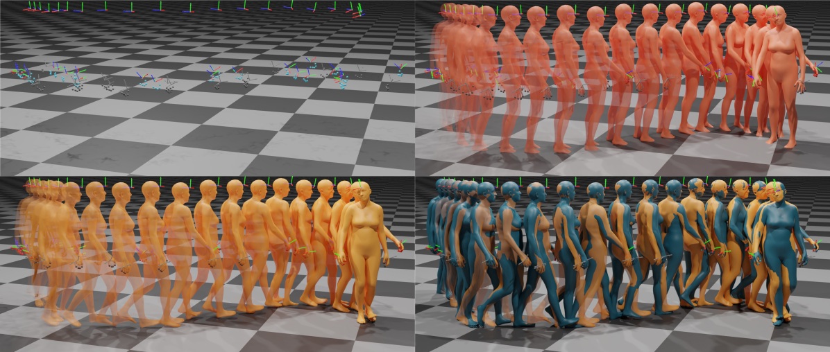
Figure 1: Top: Head and hand tracking signals from AR/VR devices (left) and the corresponding body model fit obtained from regression followed by iterative mathematical optimization. Bottom: Body model fit obtained from our learned optimizer (left), overlaid with the ground-truth (right). Learned optimizers are fast, able to tightly fit the input data and require significantly less manual labor to achieve this result. All results are estimated independently per-frame.

1 Introduction

Fitting parametric models [21, 61, 58, 78, 35, 3] to noisy input data is one of the most common tasks in computer vision. Notable examples include fitting 3D body [9, 40, 42, 58, 75, 15, 23], face [21], and hands [5, 10, 28, 66].

Direct regression using neural networks is the de facto default tool to estimate model parameters from observations. While the obtained predictions are robust and accurate to a large extent, they often fail to tightly fit the observations [85] and require large quantities of annotated data. Classic optimization methods, e.g. the Levenberg–Marquardt (LM) algorithm [44, 51], can tightly fit the parametric model to the data by iteratively minimizing a hand-crafted energy function, but are prone to local minimas and require good starting points for fast convergence. Hence, practitioners combine these two approaches to benefit from their complementary strengths, initializing the model parameters from a regressor, followed by energy minimization using a classic optimizer.

If we look one level deeper, optimization-based model fitting methods have another disadvantage of often requiring hand-crafted energy functions that are difficult to define and non-trivial to tune. Besides the data terms, each fitting problem effectively requires the definition of their own prior terms and regularization terms. Besides the work required to formulate these terms and train the priors, domain experts needs to spend significant amounts of time to balance the effect of each term. Since these priors are often hand-defined or assumed to follow distributions that are tractable / easy to optimize, the resulting fitting energy usually contains biases that can limit the accuracy of the resulting fits.

To get the best of both regression using deep learning and classical numerical optimization, we turn to the field of machine learning based continuous optimization [63, 64, 16, 2, 67, 84]. Here, instead of updating the model parameters using a first or second order model fitter, a network learns to iteratively update the parameters that minimize the target loss, with the added benefit of optimized ML back-ends for fast inference. End-to-end network training removes the need for hand-crafted priors, since the model learns them directly from data.

Inspired by the properties of the popular Levenberg–Marquardt and Adam [38] algorithms, our main contribution extends the system presented in [67] with an iterative machine learning solver which (i) keeps information from previous iterations, (ii) controls the learning rate of each variable independently and (iii) combines updates from gradient descent and from a network that is capable of swiftly reducing the fitting energy, for robustness and convergence speed. We evaluate our approach on different challenging scenarios: full-body tracking from head and hand inputs only, e.g. given by a device like the HoloLens 2, body estimation from 2D keypoints and face tracking from 2D landmarks, demonstrating both high quality results and versatility of the proposed framework.

2 Related Work

Learning to optimize [63, 64, 2] is a field that, casts optimization as a learning problem. The goal is to create models that learn to exploit the problem structure, producing faster and more effective energy minimizers. In this way, we can remove the need for hand-designed parameter update rules and priors, since we can learn them directly from the data. This approach has been used for image denoising and depth-from-stereo estimation [73], rigid motion estimation [47], view synthesis [24], joint estimation of motion and scene geometry [16], non-linear tomographic inversion problem with simulated data [1], face alignment [77] and object reconstruction from a single image [41].

Parametric human model fitting: The seminal work of Blanz and Vetter [8] introduced a parametric model of human faces and a user-assisted method to fit the model to images. Since then, the field has evolved and produced better face models and faster, more accurate and more robust estimation methods [21]. With the introduction of SMPL [46], the field of 3D body pose and shape estimation has been rapidly progressing. The community has created large motion databases [48] from motion capture data, as well as datasets, both real and synthetic, with images and corresponding 3D body ground-truth [50, 57, 27]. Thanks to these, we can now train neural network regressors that can reliably predict SMPL parameters from images [34, 36, 42, 85, 43, 45] and videos [14, 39]. With the introduction of expressive models [35, 58, 78], the latest regression approaches [15, 62, 23] can now predict the 3D body, face and hands. However, one common issue, present in all regression scenarios, is the misalignment of the predictions and the input data [85, 65]. Thus, they often serve as the initial point for an optimization-based method [9, 58, 75], which refines the estimated parameters until some convergence criterion is met. This combination produces system that are effective, robust and able to work in real-time and under challenging conditions [69, 66, 52]. These hybrid regression-optimization systems are also effective pseudo annotators for in-the-wild images [42], where standard capture technologies are not applicable. However, formulating the correct energy terms and finding the right balance between them is a challenging and time-consuming task. Furthermore, adapting the optimizer to run in real-time is a non-trivial operation, even when using popular algorithms such as the Levenberg–Marquardt algorithm [44, 51, 32] which has a cubic complexity. Thus, explicitly computing the Jacobian [16, 47] is often prohibitive in practice, either in terms of memory or runtime. The most common and practical way to speedup the optimization is to utilize the sparsity of the problem or make certain assumptions to simplify it [22]. Learned optimizers promise to overcome these issues, by learning the parametric model priors directly from the data and taking more aggressive steps, thus converging in fewer iterations. The effectiveness of these approaches has been demonstrated in different scenarios, such as fitting a body model [46, 78] to images [67, 84] and videos [82], to sparse sensor data from electromagnetic sensors [37] and multi-body estimation from multi-view images [19].

We propose a new update rule, computed as a weighted combination of the gradient descent step and the network update [67], where their relative weights are a function of the residuals. Many popular optimizers have an internal memory, such as Adam’s [38] running averages, Clark et al.’s [16] and Neural Descent’s [84] RNN. We adopt this insight, using an RNN to predict the network update and the combination weights. The network can choose to follow either the gradient or the network direction more, using both current and past residual values.

Estimating 3D human pose from a head-mounted device is a difficult problem, due to self-occlusions caused by the position of the headset and the sparsity of the input signals [79]. Yuan and Kitani [81, 80] cast this as a control problem, where a model learns to produce target joint angles for a Proportional-Derivative (PD) controller. Other methods [72, 71] tackle this as a learning problem, where a neural network learns to predict the 3D pose from the cameras mounted on the HMD. Guzov et al. [26] use sensor data from IMUs placed on the subject’s body and combine them with camera self-localization. They formulate an optimization problem with scene constraints, enabling the capture of long-term motions that respect scene constraints, such as foot contact with the ground. Finally, Dittadi et al. [18] propose a likelihood model that maps head and hand signals to full body poses. In our work, we focus on this scenario and empirically show that the proposed optimizer rule is competitive, both with a classic optimization baseline and a state-of-the-art likelihood model [18].

3 Method

3.1 Neural Fitter

Levenberg–Marquardt (LM) [44, 51, 32] and Powell’s dog leg method (PDL) [59] are examples of popular iterative optimization algorithms used in applications that fit either faces or full human body models to observations. These techniques employ the Gauss-Newton algorithm for both its convergence rate approaching the quadratic regime and its computational efficiency, enabling real-time model fitting applications, e.g. generative face [70, 88] and hand [69, 66] tracking. For robustness, LM and PDL both combine the Gauss-Newton algorithm and gradient descent, leading to implicit and explicit trust region being used when calculating updates, respectively. In LM, the relative contribution of the approximate Hessian and the identity matrix is weighted by a single scalar that is changing over iterations with its value carried over from one iteration to the next. Given an optimization problem over a set of parameters $\Theta$, LM computes the parameter update $\Delta\bm{\Theta}$ as the solution of the system $(J^{T}J+\lambda\text{diag}(J^{T}J))\Delta\bm{\Theta}=J^{T}\mathcal{R}$, where $J$ is the Jacobian and $\mathcal{R}$ are the current residual values. It is interesting to note that several popular optimizers, including ADAGRAD [20] and Adam [38], also carry over information about previous iteration(s), in this case to help control the learning rate for each parameter.

Inspired by the success of these algorithms, we aim at constructing a novel neural optimizer that (a) is easily applicable to different fitting problems, (b) can run at interactive rates without requiring significant efforts, (c) does not require hand crafted priors. (d) carries over information about previous iterations of the solve, (e) controls the learning rate of each parameter independently, (f) for robustness and convergence speed, combines updates from gradient descent and from a method capable of very quickly reducing the fitting energy. Note that the Learned Gradient Descent (LGD) proposed in [67] achieves (a), (b), and (c), but does not consider (d), (e), and (f). As demonstrated experimentally in Section 4, each of these additional properties leads to improved results compared to [67], and the best results are achieved when combined together.

Algorithm 1 Neural fitting

Input data $D$

$\bm{\Theta}_{0}=\Phi\left(D\right)$

$h_{0}=\Phi_{h}\left(D\right)$

while not converged do

     $\Delta\bm{\Theta}_{n},h_{n}\leftarrow f([\bm{g}_{n-1},\bm{\Theta}_{n-1}],D,h_{n-1})$

     $\bm{\Theta}_{n}\leftarrow\bm{\Theta}_{n-1}+u\left(\Delta\bm{\Theta}_{n},\bm{g}_{n-1},\bm{\Theta}_{n-1}\right)$

end while

Our proposed neural fitter estimates the values of the parameters $\bm{\Theta}$ by iteratively updating an initial estimate $\bm{\Theta}_{0}$, see Algorithm 1. While the initial estimate $\bm{\Theta}_{0}$ obtained from a deep neural network $\Phi$ might be sufficiently accurate for some applications, we will show that a careful construction of the update rule ($u(.)$ in Alg. 1) leads to significant improvements after only a few iterations. It is important to note that we do not focus on building the best possible initializer $\Phi$ for the fitting tasks at hand, which is the focus of e.g. VIBE [39] and SPIN [42]. That being said, note that these regressors could be leveraged to provide $\bm{\Theta}_{0}$ from Alg. 1. $h_{0}$ and $h_{n}$ are the hidden states of the optimization process. At the $n$-th iteration in the loop of Alg. 1, we use a neural network $f$ to predict $\Delta\bm{\Theta}_{n}$, and then apply the following update rule:

$$u(\Delta\bm{\Theta}_{n},\bm{g}_{n-1},\bm{\Theta}_{n-1})=\bm{\lambda}\Delta\bm{\Theta}_{n}+(-\bm{\gamma}\bm{g}_{n-1})$$ (1)

$$\bm{\lambda},\bm{\gamma}=f_{\bm{\lambda},\gamma}(\mathcal{R}(\bm{\Theta}_{n-1}),\mathcal{R}(\bm{\Theta}_{n-1}+\Delta\bm{\Theta}_{n})),\bm{\lambda},\bm{\gamma}\in\mathbb{R}^{\lvert\bm{\Theta}\rvert}$$ (2)

Note that LGD [67] is a special case of Eq. 1, with $\lambda=1,\gamma=0$, and with no knowledge preserved across fitting iterations. $\bm{g}_{n}$ is the gradient of the target data term w.r.t. to the problem parameters: $\bm{g}_{n}=\nabla\mathcal{L}^{D}$.

The proposed neural fitter satisfies the requirements (a), (b) and (c) in a similar fashion to LGD [67]. In the following, we describe how the properties (d), (e), and (f) outlined earlier in this section are satisfied.

(d): keeping track of past iterations. The functions $f,f_{\bm{\lambda},\bm{\gamma}}$ are implemented with a Gated Recurrent Unit (GRU) [13]. Unlike previous work, where the learned optimizer only stores past parameter values and the total loss [84], leveraging GRUs allows to learn an abstract representation of the knowledge that is important to use and forget about the previous iteration(s), and of the knowledge about the current iteration that should be preserved.

(e): independent learning rate. When fitting face or body models to data, the variables being optimized over are of different nature. For instance, rotations might be expressed in Euler angles while translation in meters. Since each of these parameter has a different scale and / or unit, it is useful to have per-parameter step size values. Here, we propose to predict vectors $\lambda$ and $\gamma$ independently to scale the relative contribution of $\Delta\bm{\Theta}_{n}$ and $\bm{g}_{n}$ to the update applied to each entry of $\bm{\Theta}_{n}$. It is interesting to note that $f_{\lambda}$ having knowledge about the current value of residuals at $\bm{\Theta}_{n}$ and the residual at $\bm{\Theta}_{n}+\Delta\bm{\Theta}_{n}$, effectively makes use of an estimate of the step direction before setting a step size which is analogous to how line-search operates. Motivated by this observation we tried a few learned versions of line search which yielded similar or inferior results to what we propose here. The alternatives we tried are described in the Sup. Mat..

(f): combining gradient descent and network updates. LM interpolates between Gradient Descent (GD) and Gauss-Newton (GN) using an iteration dependent scalar. LM combines the benefits of both approaches, namely fast convergence near the minimum like GN and large descent steps away from the minimum like GD. In this work, we replace the GN direction, which is often prohibitive to compute, with a network-predicted update, described in Eq. 1. The neural optimizer should learn the optimal descent direction and the relative weights to minimize the data term in as few steps as possible. In the Sup. Mat. we provide alternative combinations, e.g. via convex combination, which yielded inferior results in our experiments.

3.2 Human Body Model and Fitting Tasks

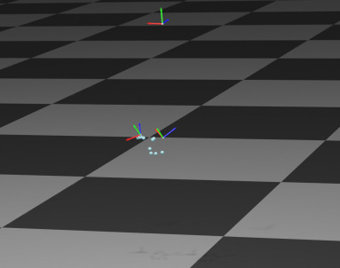
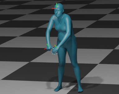
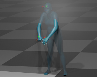
Figure 2: Left to right: 1) Input 6-DoF transformations $T_{\mathtt{H}},T_{\mathtt{L}},T_{\mathtt{R}}$ and fingertip positions $P_{i=1,\ldots 5}^{\mathtt{L}},P_{i=1,\ldots 5}^{\mathtt{R}}$, given by the head-mounted device, 2) ground-truth mesh, 3) half-space visibility, everything behind the headset is not visible.

We represent the human body using SMPL [46]/SMPL+H [61], a differentiable function that computes mesh vertices $M(\bm{\theta},\bm{\beta})\in\mathbb{R}^{\mathtt{V}\times 3}$, $\mathtt{V}=6890$, from pose $\bm{\theta}$ and shape $\bm{\beta}$, using standard linear blend skinning (LBS). The 3D joints, $\mathcal{J}(\bm{\beta})$, of a kinematic skeleton are computed from the shape parameters. The pose parameters $\bm{\theta}\in\mathbb{R}^{\mathtt{J}\times\mathtt{D}+3}$ contain the parent-relative rotations of each joint and the root translation, where $\mathtt{D}$ is the dimension of the rotation representation and $\mathtt{J}$ is the number of skeleton joints. We represent rotations using the 6D rotation parameterization of Zhou et al. [87], thus $\theta\in\mathbb{R}^{\mathtt{J}\times 6+3}$. The world transformation $T_{j}(\bm{\theta})\in SE(3)$ of each joint $j$ is computed by following the transformations of its parents in the kinematic tree: $T_{j}(\bm{\theta})=T_{p(j)}(\bm{\theta})*T\left(\bm{\theta}_{j},\mathcal{J}_{j}(\bm{\beta})\right)$, where $p(j)$ is the index of the parent of joint $j$ and $T\left(\bm{\theta}_{j},\mathcal{J}_{j}(\bm{\beta})\right)$ is the rigid transformation of joint $j$ relative to its parent. Variables with a hat denote observed quantities.

We focus on two 3D human body estimation problems: 1) fitting a body model [46] to 2D keypoints and 2) inferring the body, including hand articulation [61], from head and hand signals returned by AR/VR devices, shown in Fig. 2. The first is by now a standard problem in the Computer Vision community. The second, which uses only head and hand signals in the AR/VR scenario, is a significantly harder task which requires strong priors, in particular to produce plausible results for the lower body and hands. The design of such priors is not trivial, requires expert knowledge and a significant investment of time.
2D keypoint fitting: We follow the setup of Song et al. [67], computing the projection of the 3D SMPL joints $\mathcal{J}$ with a weak-perspective camera $\Pi$ with scale $s\in\mathbb{R}{}$, translation $\bm{t}\in\mathbb{R}^{2}$: $\mathtt{j}=\Pi_{o}(\mathcal{J}(\bm{\theta},\bm{\beta}),s,\bm{t})$. Our goal is to estimate SMPL and camera parameters $\bm{\Theta}^{B}=\{\bm{\theta},\bm{\beta}\}$, $\mathrm{K}^{B}=\{s,\bm{t}\}$, such that the projected joints $\mathtt{j}$ match the detected keypoints $D^{B}=\{\hat{\mathtt{j}}\}$, e.g. from OpenPose [11]. Fitting SMPL+H to AR/VR device signals: We make the following assumptions: 1. the device head tracking system provides a 6-DoF transformation $\hat{T}^{\mathtt{H}}$, that contains the position and orientation of the headset in the world coordinate frame. 2. the device hand tracking system gives us the orientation and position of the left and right wrist, $\hat{T}^{\mathtt{L}},\hat{T}^{\mathtt{R}}\in SE(3)$, and the positions of the fingertips $\hat{P}_{1,\ldots,5}^{\mathtt{L}},\hat{P}_{1,\ldots,5}^{\mathtt{R}}\in\mathbb{R}^{3}$ in the world coordinate frame, if and when they are in the field of view (FOV) of the HMD. In order to estimate the SMPL+H parameters that best fit the above observations, we compute the estimated headset position and orientation from the SMPL+H world transformations as $T^{\mathtt{H}}(\bm{\Theta})=T^{\text{\mbox{HMD}}}T_{j_{\mathtt{H}}}(\bm{\Theta})$, where $j_{\mathtt{H}}$ is the index of the head joint of SMPL+H. $T^{\text{\mbox{HMD}}}$ is a fixed transform from the SMPL+H head joint to the headset, obtained from an offline calibration phase.
Visibility is represented by $v_{\mathtt{L}},v_{\mathtt{R}}\in\{0,1\}$ for the left and right hand respectively. We examine two scenarios: 1. full visibility, where the hands are always visible, 2. half-space visibility, where only the area in front of the HMD is visible. Specifically, we transform the points into the coordinate frame of the headset, using $T^{\mathtt{H}}$. All points with $z\geq 0$ are behind the headset and thus invisible. Fig. 2 right visualizes the plane that defines what is visible or not.
To sum up, the sensor data are: $D^{\text{\mbox{HMD}}}=\{\hat{T}^{\mathtt{H}},\hat{T}^{\mathtt{L}},\hat{T}^{\mathtt{R}},\hat{P}_{i=1,\ldots,5}^{\mathtt{L}},\hat{P}_{i=1,\ldots,5}^{\mathtt{R}},v_{\mathtt{L}},v_{\mathtt{R}}\}$. The goal is to estimate the parameters $\bm{\Theta}^{\text{\mbox{HMD}}}=\left\{\bm{\theta}\right\}\in\mathbb{R}^{315}$, that best fit $D^{\text{\mbox{HMD}}}$. Note that we assume we are given body shape $\bm{\beta}$ for the HMD fitting scenario.

3.3 Human Face Model and Fitting Task

We represent the human face using the parametric face model proposed by Wood et al. [74]. It is a blendshape model [21], with $\mathtt{V}=7667$ vertices, 4 skeleton joints (head, neck and two eyes), with their rotations and translations denoted with $\bm{\theta}$, identity $\bm{\beta}\in\mathbb{R}^{256}$ and expression $\bm{\psi}\in\mathbb{R}^{233}$ blendshapes. The deformed face mesh is obtained with standard linear blend skinning.

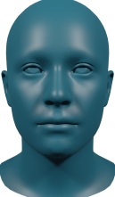
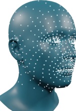
Figure 3: Blue: The face model template of Wood et al. [74]. White: 669 dense landmarks.

For face fitting, we select a set of mesh vertices as the face landmarks $\mathcal{P}(\bm{\theta},\bm{\psi},\bm{\beta})\in\mathbb{R}^{\mathtt{P}\times 3}$, $\mathtt{P}=669$ (see Fig. 3 right). The input data are the corresponding 2D face landmarks $\hat{p}\in\mathbb{R}^{\mathtt{P}}\times 2$, detected using the landmark neural network proposed by Wood et al. [74].

For this task, our goal is to estimate translation, joint rotations, expression and identity coefficients $\bm{\Theta}^{F}=\left\{\bm{\theta},\bm{\psi},\bm{\beta}\right\}\in\mathbb{R}^{516}$ that best fit the 2D landmarks $D^{F}=\hat{p}$. We assume we are dealing with calibrated cameras and thus have access to the camera intrinsics $\mathrm{K}$. $\Pi_{p}(\mathcal{P};\mathrm{K})$ is the perspective camera projection function used to project the 3D landmarks $\mathcal{P}$ onto the image plane.

3.4 Data Terms

The data term is a function $\mathcal{L}^{D}(\bm{\Theta};D)$ that measures the discrepancy between the observed inputs $D$ and the parametric model evaluated at the estimated parameters $\bm{\Theta}$.

At the $n$-th iteration of the fitting process, we compute both 1) the array $\mathcal{R}(\bm{\Theta}_{n})$ that contains all the corresponding residuals of the data term $\mathcal{L}^{D}$ for the current set of parameters $\bm{\Theta}_{n}$, and 2) the gradient $\bm{g}_{n}=\nabla\mathcal{L}^{D}(\bm{\Theta}_{n})$.

Let $\llbracket\rrbracket$ by any metric appropriate for $SE(3)$ [18] and $\lVert\rVert_{\psi}$ a robust norm [6]. To compute residuals, we use the Frobenius norm for $\llbracket\rrbracket$ and $\lVert\rVert_{\psi}$ Note that any other norm choice can be made compatible with LM [83].

Body fitting to 2D keypoints: We employ the re-projection error between the detected joints and those estimated from the model as the data term:

$$\mathcal{L}^{D}(\bm{\Theta}^{B};D^{B})=\lVert\hat{\mathtt{j}}-\Pi_{p}\left(\mathcal{J}(\bm{\Theta}^{B}),\mathrm{K}^{B}\right)\rVert_{\psi}$$ (3)

Here $\mathcal{J}(\bm{\Theta}^{B})$ denotes the “posed” joints.

Body fitting to HMD signals: We measure the discrepancy between the observed data $D^{\text{\mbox{HMD}}}$ and the estimated model parameters $\bm{\Theta}^{\text{\mbox{HMD}}}$ with the following data term:

$$\mathcal{L}^{D}(\bm{\Theta}^{\text{\mbox{HMD}}};D^{\text{\mbox{HMD}}})=\llbracket\hat{T}^{\mathtt{H}},T^{\mathtt{H}}(\bm{\Theta}^{\text{\mbox{HMD}}})\rrbracket+$$ (4)

$$\sum_{w\in{\mathtt{L},\mathtt{R}}}v_{w}\left(\llbracket\hat{T}^{w},T^{w}(\bm{\Theta}^{\text{\mbox{HMD}}})\rrbracket+\sum_{i=1}^{5}\lVert\hat{P}_{i}^{w}-P_{i}^{w}(\bm{\Theta}^{\text{\mbox{HMD}}})\rVert_{\psi}\right)$$

Face fitting to 2D landmarks: The data term is the landmark re-projection error:

$$\mathcal{L}^{D}(\bm{\Theta}^{F};D^{F})=\lVert\hat{p}-\Pi_{p}\left(\mathcal{P}(\bm{\Theta}^{F});\mathrm{K}^{F}\right)\rVert_{\psi}$$ (5)

3.5 Training Details

Training losses: We train our learned fitter using a combination of model parameter and mesh losses. Their precise formulation can be found in the Sup. Mat.

Model structure: Unless otherwise specified, $f,f_{\bm{\lambda},\bm{\gamma}}$ (in Alg. 1, (2)) use a stack of two GRUs with 1024 units each. The initialization $\Phi,\Phi_{h}$ in Alg. 1 are MLPs with two layers of 256 units, ReLU [54] and Batch Normalization [33].

Datasets: For the body fitting tasks, we use AMASS [48] to train and test our fitters. When fitting SMPL to 2D keypoints, we use 3DPW’s [50] test set to evaluate the learned fitter’s accuracy, using the detected OpenPose [11] keypoints as the target. The face fitter is trained and evaluated on synthetic data. Please see the Sup. Mat. for more details on the datasets.

4 Experiments

4.1 Metrics

Metrics with a PA prefix are computed after undoing rotation, scale and translation, i.e. Procrustes alignment. Variables with a tilde are ground-truth values.

Vertex-to-Vertex (V2V): As we know the correspondence between ground-truth $\tilde{M}$ and estimated vertices $M$, we are able to compute the mean per-vertex error: $\mbox{V2V}(\tilde{M},M)=\frac{1}{\mathtt{V}}\sum_{i=1}^{\mathtt{V}}\lVert\tilde{M}_{i}-M_{i}\rVert_{2}$. For SMPL+H, in addition to the full mesh error (FB), we report error values for the head (H) and hands (L, R). A visualization of the selected parts is included in the Sup. Mat. The 3D per-joint error (JntErr) is equal to: $\mbox{JntErr}(\tilde{\mathcal{J}},\mathcal{J})=\frac{1}{\mathtt{J}}\sum_{i=1}^{\mathtt{J}}\lVert\tilde{\mathcal{J}}_{i}-\mathcal{J}_{i}\rVert_{2}$.

Ground penetration (GrPe.): We report the average distance to the ground plane for all vertices below ground [82]: $\text{GrPe.}(M)=\frac{1}{\lvert\mathtt{S}\rvert}\sum_{n\in\mathtt{S}}\lvert d_{\text{gnd}}(M_{i})\rvert$, where $d_{\text{gnd}}({M}_{i})=M_{i}\cdot n_{\text{gnd}}$ and $\mathtt{S}=\{i\mid d_{\text{gnd}}(M_{i})<0\}$.

Face landmark error (LdmkErr): We report the mean distance between estimated and ground-truth 3D landmarks $\mbox{LdmkErr}(\tilde{\mathcal{P}},\mathcal{P})=\frac{1}{\mathtt{P}}\sum_{i=1}^{\mathtt{P}}\lVert\tilde{\mathcal{P}}_{i}-\mathcal{P}_{i}\rVert_{2}$.

Table 1: Using 3DPW [50] to compare different approaches that estimate SMPL from images, 2D keypoints and part segmentation masks. Replacing LGD’s [67] update rule with ours leads to a 2 mm PA-MPJPE improvement. Our full system, that uses GRUs, leads to a further 1.6 mm improvement. “O/R” denotes Optimization/Regression.

Method	Type	Image	2D keypoints	Part segmentation	PA-MPJPE
SMPLify [9]	O	✗	✓	✗	106.1
SCOPE [22]	O	✗	✓	✗	68.0
SPIN [42]	R	✓	✗	✗	59.6
VIBE [39]	R	✓	✗	✗	55.9
Neural Descent [84]	R+O	✓	✓	✓	57.5
LGD [67]	R+O	✗	✓	✗	55.9
Ours, LGD + Eq. 1	R+O	✗	✓	✗	53.9
Ours (full)	R+O	✗	✓	✗	52.2

4.2 Quantitative Evaluation

Table 2: Fitting SMPL+H to simulated sequences of HMD data. Our proposed fitter outperforms the classical optimization baselines (L-BFGS prefix) on the full body and ground penetration metrics, with similar or better performance on the part metrics, and the regressor baselines (the VAE predictor [18] and the regressor $\Phi$), on all metrics. “F/H” denotes full / half-plane visibility.

	Vertex-to-vertex (mm) $\downarrow$						JntErr		GrPe.
Method	Full body		Head		L / R hand		(mm) $\downarrow$		(mm) $\downarrow$
	F	H	F	H	F	H	F	H	F	H
L-BFGS, GMM	73.1	116.2	2.9	3.4	3.2 / 3.0	5.6 / 5.3	49.7	137.26	70.8	74.0
L-BFGS, GMM, Tempo.	72.6	113.3	2.9	3.4	3.3 / 3.1	6.8 / 6.5	49.4	132.1	70.7	73.5
L-BFGS, VAE Enc.	76.1	119.3	3.9	4.1	5.3 / 4.7	8.7 / 7.6	52.6	140.5	63.6	66.7
Dittadi et al. [18]	n/a		n/a		n/a		43.3	n/a	n/a
Ours $\Phi,(N=0)$	44.2	69.7	19.1	22.7	27.8 / 25.9	32.1 / 29.9	38.9	84.9	16.1	20.1
Ours $(N=5)$	26.1	49.9	2.2	3.2	3.0 / 3.3	3.1 / 3.7	18.1	62.1	12.5	15.5

Fitting the body to 2D keypoints: We compare our proposed update rule with existing regressors, classic and learned optimization methods on 3DPW [50]. For a fairer comparison with Song et al. [67], we train two versions of our proposed fitter, one where we change the update rule of LGD with Eq. 1, and our full system which also has network architecture changes. Table 1 shows that just by changing the update rule (Ours, LGD + Eq. 1), we outperform all baselines.
Fitting the body to HMD data: In Tab. 2 we compare our proposed learned optimizer with a standard optimization pipeline, a variant of SMPLify [9, 58] adapted to the HMD fitting task (first 3 rows), and two neural network regressors (a VAE predictor [18] in the 4th row and our initializer $\Phi$ of Alg. 1 in the 5th row), on the task of fitting SMPL+H to sparse HMD signals, see Sec. 3.2. The optimization baseline minimizes the energy with data term ($\mathcal{L}^{D}$ in Eq. 4), gravity term $\mathcal{L}^{\mathcal{G}}$, prior term $\mathcal{L}^{\bm{\theta}}_{\text{prior}}$, without/with temporal term $\mathcal{L}^{\mathrm{T}}$ (first/second row of Tab. 2) to estimate the parameters $\bm{\Theta}_{1,\ldots,\mathrm{T}}$ of a sequence of length $\mathrm{T}$:

$$\mathcal{L}^{\mathcal{O}}(\bm{\Theta}^{\text{\mbox{HMD}}})=\mathcal{L}^{D}(\bm{\Theta}^{\text{\mbox{HMD}}};D^{\text{\mbox{HMD}}})+\mathcal{L}^{\mathcal{G}}+\mathcal{L}^{\bm{\theta}}_{\text{prior}}+\mathcal{L}^{\mathrm{T}}$$ (6)

$$\mathcal{L}^{\mathcal{G}}(\bm{\Theta}^{\text{\mbox{HMD}}})=1-\frac{T_{\text{pelvis}}(1,:3)\cdot\bm{\mathrm{u}}}{\lVert T_{\text{pelvis}}(1,:3)\rVert_{2}\lVert{\bm{\mathrm{u}}}\rVert_{2}},\,\bm{\mathrm{u}}=(0,1,0)$$

$$\mathcal{L}^{\mathrm{T}}(\bm{\Theta}^{\text{\mbox{HMD}}})=\sum_{t=1}^{\mathrm{T}-1}\llbracket T_{t+1}(\bm{\Theta}_{t+1}^{\text{\mbox{HMD}}})-T_{t}(\bm{\Theta}_{t}^{\text{\mbox{HMD}}})\rrbracket$$

We use two different pose priors, a GMM [9] and a VAE encoder $\mathcal{E}(*)$ [58]:

$$\mathcal{L}^{\bm{\theta}}_{\text{GMM}}=-\min_{j}{\log{\left(w_{j}\mathcal{N}(\bm{\theta};\mu_{\bm{\theta},j},\Sigma_{\bm{\theta},j})\right)}}$$ (7)

$$\mathcal{L}^{\bm{\theta}}_{\text{VAE}}=\text{Neg. Log-Likelihood}(\mathcal{N}(\mathcal{E}(\bm{\theta}),\mathcal{I}))$$ (8)

We minimize the loss above using L-BFGS [55, Ch. 7.2] for 120 iterations on the test split of the MoCap data. We choose L-BFGS instead of Levenberg-Marquardt, since PyTorch currently lacks the feature to efficiently compute jacobians, without having to resort to multiple backward passes for derivative computations. We report the results for both full and half-space visibility in Tab. 2 using the metrics of Section 4.1. Our method outperforms the baselines in terms of full-body and penetration metrics, and shows competitive performance w.r.t. to the part metrics. Regression-only methods [18] cannot tightly fit the data, due to the lack of a feedback mechanism.

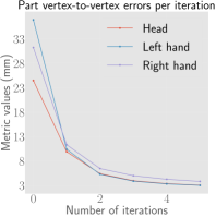
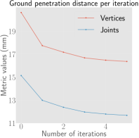
Figure 4: Errors per iteration when fitting SMPL+H to HMD data for the half-space visibility scenario, see Sup. Mat. for full visibility. Left to right: 1) full body vertex and joint errors, 2) head, left and right hand V2V errors and 3) vertex and joint ground distance, computed on the set of points below ground.

Runtime: Our method (PyTorch) runs at 150 ms per frame on a P100 GPU, while the baseline L-BFGS method (PyTorch) above requires 520 ms, on the same hardware. We are aware that a highly optimized real-time version of the latter exists and runs at 0.8 ms per frame, performing at most 3 LM iterations, but it requires investing significant effort into a problem specific C++ codebase.

Fig. 4 contains the metrics per iteration of our method, averaged across the entire test dataset. It shows that our learned fitter is able to aggressively optimize the target data term and converge quickly.

Table 3: Using per-step network weights reduces head and ground penetration errors, albeit at an N-folder parameter increase. Weights V2V (mm) $\downarrow$ JntErr GrPe. FB H L / R (mm) $\downarrow$ (mm)$\downarrow$ Shared 52.3 3.5 3.6 / 3.7 64.1 18.2 Per-step 49.9 3.2 3.1 / 3.7 62.1 15.5 Table 4: GRU vs a residual feed-forward network [29, 68]. GRU’s memory makes it more effective. Multiple layers bring further benefits, but increase runtime. Network V2V (mm) $\downarrow$ JntErr GrPe. Structure FB H L / R (mm) $\downarrow$ (mm)$\downarrow$ ResNet 65.3 6.8 7.3 / 7.6 73.1 16.2 GRU (1024) 53.6 3.7 3.4 / 4.0 66.1 15.1 GRU (1024, 1024) 49.9 3.2 3.1 / 3.7 62.1 15.5

Table 5: Comparison of our update rule (Eq. 1) with the pure network update $\Delta\Theta_{n}$. Our proposed combination improves the results for all metrics. Update V2V (mm) $\downarrow$ JntErr GrPe. Rule FB H L / R (mm) $\downarrow$ (mm)$\downarrow$ +$\Delta\Theta_{n}$ 53.8 14.7 7.8 / 7.9 66.3 15.8 +Eq. 1 49.9 3.2 3.1 / 3.7 62.1 15.5 Table 6: Learning to predict $\gamma$ is better than a constant, with performance degrading gracefully, providing an option for a lower computational cost. Learning V2V (mm) $\downarrow$ JntErr GrPe. rate $\bm{\gamma}$ FB H L / R (mm) $\downarrow$ (mm)$\downarrow$ 1e-4 51.9 3.5 3.8 / 4.6 64.2 15.5 Learned 49.9 3.2 3.1 / 3.7 62.1 15.5

Ablation study: We perform our ablations on the problem of fitting SMPL+H to HMD signals, using the half-space visibility setting. Unless otherwise stated, we report the performance of regression and 5 iterations of the learned fitter.

We first compare two variants of the fitter, one with shared and the other with separate network weights per optimization step. Table 4 shows that the latter can help reduce the errors, at the cost of an N-fold increase in memory.

Secondly, we investigate the effect of the type and structure of the network, replacing the GRU with a feed-forward network with skip connections, i.e., ResNet [29, 68]. We also train a version of our fitter with a single GRU with 1024 units. Table 4 shows that the GRU is better suited to this type of problem, thanks to its internal memory. This is very much in line with many popular continuous optimizer work [84].

Thirdly, we compare the update rule of Eq. 1 with a learned fitter that only uses the network update, i.e. $\bm{\gamma}=0,\bm{\lambda}=1$ in Eq. 1. This is an instantiation of LGD [67], albeit with a different network and task. Table 6 shows that the proposed weighted combination is better than the pure network update.

Fourthly, we investigate whether we need to learn the step size $\bm{\gamma}$ or if a constant value is enough. Table 6 shows that performance gracefully degrades when using a constant learning value. Therefore, it is an option for decreasing the computational cost, without a significant performance drop.

Finally, we present some qualitative results in Fig. 6. Notice how the learned fitter corrects the head pose and hand articulation of the initial predictions.

Table 7: Face fitting to 2D landmarks.

	V2V (mm) $\downarrow$				LdmkErr
	Face		Head		(mm) $\downarrow$
Method	-	PA	-	PA	-	PA
LM	34.4	3.7	33.8	5.3	33.8	3.4
Ours	7.9	3.5	8.5	4.1	8.0	3.7

Face fitting to 2D landmarks: We compare our proposed learned optimizer with a C++ production grade solution that uses LM to solve the face fitting problem described in Sec. 3.3. Given the per-image 2D landmarks as input, the optimization baseline minimizes the energy with data term ($\mathcal{L}^{D}$ in Eq. 5) and a simple regularization term to estimate $\bm{\Theta}^{F}=\left\{\bm{\theta},\bm{\psi},\bm{\beta}\right\}$:

$$\mathcal{L}^{\mathcal{O}}(\bm{\Theta}^{F})=\mathcal{L}^{D}(\bm{\Theta}^{F};D^{F})+\mathbf{w}*\lVert\bm{\Theta}^{F}\rVert_{2}$$ (9)

$\mathbf{w}$ contains the different regularization weights for $\bm{\theta},\bm{\psi},\bm{\beta}$, which are tuned manually for the best baseline result.

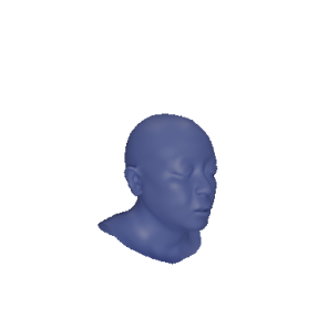
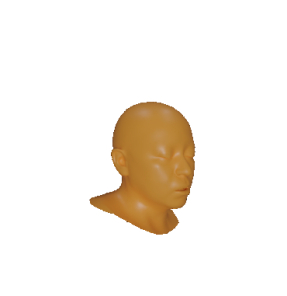
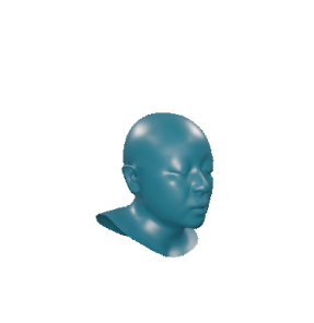
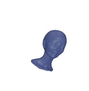
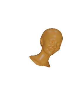
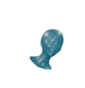
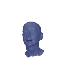
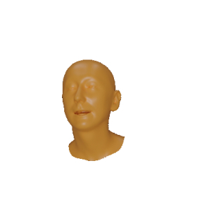
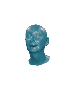
a)b)c)d)

Figure 5: Face model [74] fitting to to dense 2D landmarks a) target 2D landmarks, b) LM fitter, c) ours, d) ground-truth.

The quantitative comparison in Tab. 7 shows that our proposed fitter outperforms the LM baseline on almost all metrics. The large value in absolute errors (“-” columns) is due to the wrong estimation of the depth of the mesh. After alignment (PA columns), the gap is much smaller. See Fig. 5 for a qualitative comparison.

Runtime: Here, the baseline optimization is in C++ and thus for a fair comparison, we only compare the time it takes to compute the parameter update given the residuals and jacobians (per-iteration). Computing the values of the learned parameter update (ours, using PyTorch) takes 12 ms on a P100 GPU, while computing the LM update (baseline, C++) requires 34.7 ms ($504$ free variables). Note that the LM update only requires 0.8 ms on a laptop CPU when optimizing over $100$ free variables. The difference is due to the cubic complexity of LM w.r.t. the number of free variables of the problem.

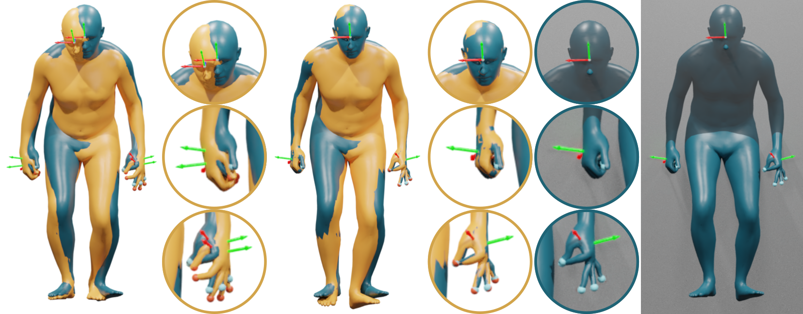
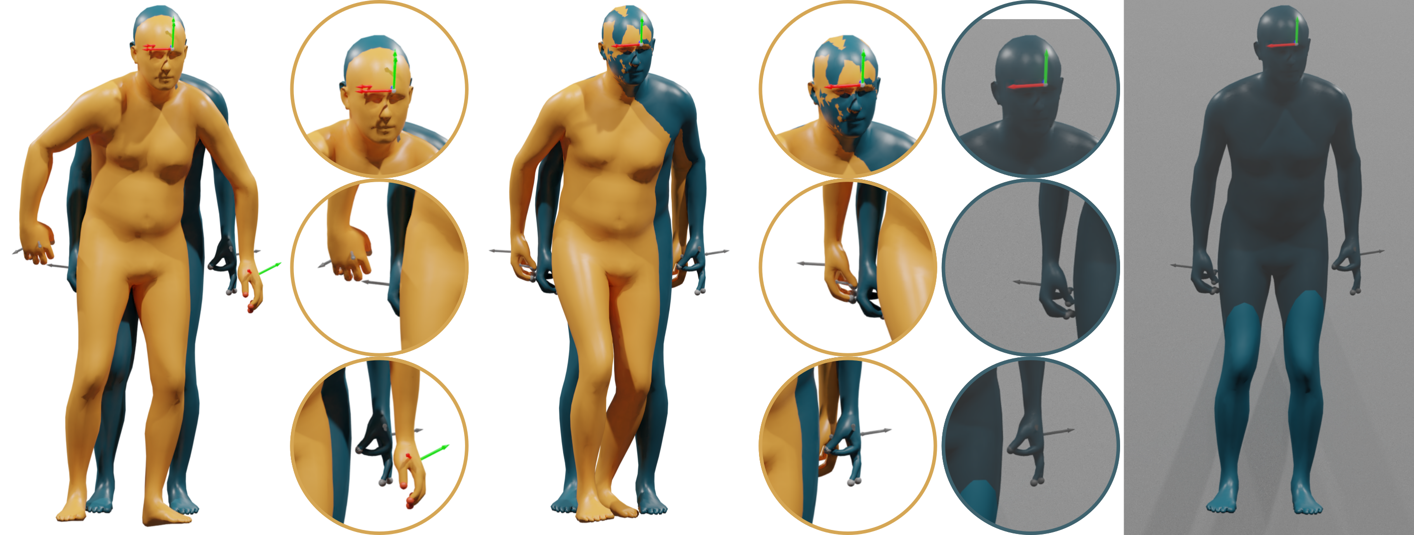
1) Initial $\Phi$ output2) Iteration $N=5$3) Ground-truth

Figure 6: Estimates in yellow, ground-truth in blue, best viewed in color. Our learned optimizer successfully fits the target data and produces plausible poses for the full 3D body. Points that are greyed out are outside of the field of view, e.g. the hands in the second row, and thus not perfectly fitted.

4.3 Discussion

If we apply the proposed method to a sequence of data, we will get plausible per-frame results, but the overall motion will be implausible. Since the model is trained on a per-frame basis and lacks temporal context, it cannot learn the proper dynamics present in temporal data. Thus, limbs in successive frames will move unnaturally, with large jumps or jitter. Future extensions of this work should therefore explore how to best use past frames and inputs. This could be coupled with a physics based approach, either as part of a controller [82] or using explicit physical losses [76, 86, 60] in $\mathcal{L}^{D}$. Another interesting direction is the use of more effective parameterizations for the per-step weights [31, 17]. While all the problems we tackle here are under-constrained and could thus have multiple solutions, the current system returns only one. Therefore, combining the proposed system with multi-modal regressors [7, 43] is another possible extension.

5 Conclusion

In this work, we propose a learned parameter update rule inspired from classic optimization algorithms that outperforms the pure network update and is competitive with standard optimization baselines. We demonstrate the utility of our algorithm on three different problem sets, estimating the 3D body from 2D keypoints, from sparse HMD signals and fitting the face to dense 2D landmarks. Learned optimizers combine the advantages of classic optimization and regression approaches. They greatly simplify the development process for new problems, since the parameter priors are directly learned from the data, without manual specification and tuning, and they run at interactive speeds, thanks to the development of specialized software for neural network inference. Thus, we believe that our proposed optimizer will be useful for any applications that involve generative model fitting.

Acknowledgement: We thank Pashmina Cameron, Sadegh Aliakbarian, Tom Cashman, Darren Cosker and Andrew Fitzgibbon for valuable discussions and proof reading.

Supplementary Material

6 Social impact

Accurate tracking is a necessary pre-requisite for the next generation of communication and entertainment through virtual and augment reality. Learned optimizers represent a promising avenue to realize this potential. However, it can also be used for surveillance and tracking of private activities of an individual, if the corresponding sensor is compromised.

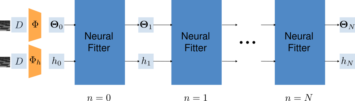
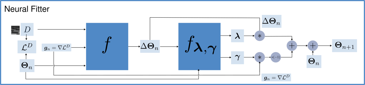
Figure A.1: Top: the general fitting process described in Alg. 1. Bottom: A schematic representation of our update rule, described in Eq. 1, 2 of the main paper.

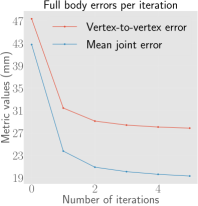
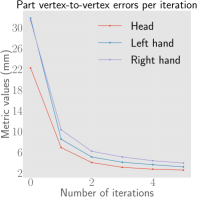
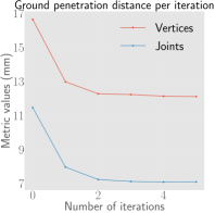
Figure A.2: Errors per iteration when fitting SMPL+H to HMD data, assuming that the hands are always visible. From left to right: 1) Full body vertex and joint errors, 2) head, left and right hand V2V errors and 3) vertex and joint ground distance, computed on the set of points below ground.

7 Errors per iteration

Figure A.2 shows the metric values per iteration, averaged across the test set, for our fitter on the task of fitting SMPL+H to HMD head and hand signals. Different to the main paper, this figure corresponds to the full visibility scenario, i.e. the hands are always visible. The learned fitter aggressively optimizes the target data term and quickly converges to the minimum.

8 Update rule

In addition to the update rule described in Eq. 1 of the main paper, we investigated two other alternatives, based on the convex combination of the network update and gradient descent. The first is a simple re-formulation of Eq. 1, with $\bm{\lambda}\in[0,1]$, selecting either the network update or the gradient descent direction. In the second, we first compute a convex combination between the normalized network update and gradient descent, i.e. selecting a direction, and then scale the computed direction according to $\bm{\gamma}$.

$$u(\Delta\bm{\Theta}_{n},\bm{g}_{n},\bm{\Theta}_{n})=\bm{\lambda}\Delta\bm{\Theta}_{n}+(1-\bm{\lambda})\left(-\bm{\gamma}\bm{g}_{n}\right)$$ (10)

$$u(\Delta\bm{\Theta}_{n},\bm{g}_{n},\bm{\Theta}_{n})=\bm{\gamma}\left[\bm{\lambda}\left(\frac{\Delta\bm{\Theta}_{n}}{\lVert\Delta\bm{\Theta}_{n}\rVert}\right)+(1-\bm{\lambda})\left(\frac{-\bm{g}_{n}}{\lVert\bm{g}_{n}\rVert}\right)\right]$$

$$\bm{\lambda}=\sigma\left(f_{\lambda}(\mathcal{R}(\bm{\Theta}_{n}),\mathcal{R}(\bm{\Theta}_{n}+\Delta\bm{\Theta}_{n})),\bm{\lambda}\in\mathbb{R}^{\lvert\bm{\Theta}\rvert}\right)$$

Here, $\sigma()$ is the sigmoid function: $\sigma(x)=\frac{1}{1+\exp{(-x)}}$. The learning rate of the gradient descent term is the same as the main text:

$$\bm{\gamma}=f_{\gamma}(\mathcal{R}(\bm{\Theta}_{n}),\mathcal{R}(\bm{\Theta}_{n}+\Delta\bm{\Theta}_{n})),\bm{\gamma}\in\mathbb{R}^{\lvert\bm{\Theta}\rvert}$$ (11)

We empirically found that the performance of these two variants is inferior to the proposed update rule, but we nevertheless list them for completeness.

9 Additional ablation

Table A.1 contains an additional ablation experiment, where we compare different options for the type of variable for $\bm{\lambda}$, $\bm{\gamma}$, namely whether to use a scalar or a vector variable, and and whether to use a common network predictor for $\bm{\lambda}$, $\bm{\gamma}$. We use the problem of fitting SMPL to 2D keypoint predictions, evaluating our results using the 3DPW test set.

Table A.1: Predicting vector values for $\bm{\lambda},\bm{\gamma}$ is always better than scalars. This is expected, since each variable to be optimized has different scale and the learned fitter must adapt its predicted updates accordingly. Having a shared network for $\bm{\lambda},\bm{\gamma}$ improves performance and lowers the number of parameters of the learned fitter.

Vector $\bm{\lambda}$	Vector $\bm{\gamma}$	Shared network for $\bm{\lambda},\bm{\gamma}$	PA-MPJPE (mm)
✓	✗	✗	52.8
✗	✓	✗	52.7
✓	✓	✗	52.3
✓	✓	✓	52.2

10 Qualitative comparisons

We present a qualitative comparison of the proposed learned optimizer with a classic optimization-based method in Fig. A.3. Without explicit hand-crafted constraints, the classic approach cannot resolve problems such as ground-floor penetration. Formulating a term to represent this constraint is not a trivial process. Furthermore, tuning the relative weight of this term to avoid under-fitting the data term is not a trivial process. Our proposed method on the other hand can learn to handle these constraints directly from data, without any heuristics.

11 Training details

11.1 GRU formulation

All our recurrent networks are implemented with Gated Recurrent Units (GRU) [13], with layer normalization [4]:

$$z_{n}=\sigma_{g}\left(LN(W_{z}x)+LN(U_{z}h_{n-1})\right)$$ (12)

$$r_{n}=\sigma_{g}\left(LN(W_{r}x)+LN(U_{r}h_{n-1})\right)$$

$$\hat{h}_{n}=\phi_{h}\left(LN(W_{h}x)+LN(U_{h}\left(r_{n}\odot h_{n-1}\right))\right)$$

$$h_{n}=(1-z_{n})\odot h_{n-1}+z_{n}\odot\hat{h}_{n},\quad h_{0}=\Phi_{h}\left(D\right)$$

We also tried replacing the GRUs with LSTMs [30], but did not observe significant performance benefit. Hence we chose the computationally lighter GRUs.

11.2 Training losses

We apply a loss on the output of every step of our network:

$$\mathcal{L}(\{\bm{\Theta}_{n}\}_{n=0}^{N},\{\hat{\bm{\Theta}}_{n}\}_{n=0}^{N};D)=\sum_{i=0}^{N}\mathcal{L}_{i}(\bm{\Theta}_{i},\hat{\bm{\Theta}}_{i};D)$$ (13)

The loss $\mathcal{L}_{i}$ contains the following terms:

$$\mathcal{L}_{i}=\lambda_{M}\mathcal{L}_{i}^{M}+\lambda_{\mathcal{E}}\mathcal{L}_{i}^{\mathcal{E}}+\lambda_{T}\mathcal{L}_{i}^{T}+\lambda_{\bm{\theta}}\mathcal{L}_{i}^{\bm{\theta}}$$ (14)

$$\mathcal{L}_{i}^{M}=\lVert\hat{M}-M\rVert_{1}$$ (15)

$$\mathcal{L}_{i}^{\mathcal{E}}=\sum_{(i,j)\in\mathcal{E}}\lVert(\hat{M}_{i}-\hat{M}_{j})-(M_{i}-M_{j})\rVert_{1}$$ (16)

$$\mathcal{L}_{i}^{T}=\sum_{j=1}^{J}\lVert\hat{T}_{j}-T_{j}\rVert_{1}$$ (17)

$$\mathcal{L}_{i}^{\bm{\theta}}=\lVert\hat{R}_{\bm{\theta}}-R_{\bm{\theta}}\rVert_{1}+\lVert\hat{\bm{t}}-\bm{t}\rVert_{1}$$ (18)

$M$ represents the mesh vertices deformed by parameters $\bm{\Theta}$. $\mathcal{E}$ is the set of vertex indices of the mesh edges. $T$ denotes the transformations in world coordinate while $R_{\bm{\theta}}$ denotes the rotation matrices (in the parent-relative coordinate frame) computed from the pose values $\bm{\theta}$. $\bm{t}$ is the root translation vector. We use the following values for the weights of the training losses: $\lambda_{M}=1000$, $\lambda_{\mathcal{E}}=1000$, $\lambda_{T}=100$, $\lambda_{\bm{\theta}}=1$, $\lambda_{\bm{t}}=100$.

11.3 Datasets

For body fitting from HMD signals, we use a subset of AMASS [48] to train and test our method. Specifically, we use CMU [12], KIT [49] and MPI_HDM05 [53], adopting the same pre-processing and training, test splits as [18]. An important difference is that we fit the neutral SMPL+H to the gendered SMPL+H data found in AMASS, to preserve correct contact with the ground and avoid the use of heuristics [60]. We attach random hand poses from the MANO [61] training set to simulate hand articulation. In all our experiments that involve SMPL+H, we use the ground-truth shape parameters $\bm{\beta}$. Future work could include estimating a subset of the shape parameters corresponding to height from the position of the headset. For the learned fitter that estimates body parameters from 2D joints, we use the data, augmentation and evaluation protocol of Song et al. [67]. To be more precise, we use AMASS [48] to train the fitter and evaluate the resulting model on 3DPW [50], which contains sequences of subjects in complex poses in outdoor scenes, along with SMPL parameters captured using RGB cameras and IMUs.

For face fitting from 2D landmarks, we use the face model proposed in [74] to generate a synthetic face dataset by sampling $50000$ sets of parameters from the model space. For each sample, we vary pose, identity and expression. We use a perspective camera with focal length $(512,512)$ and principal point $(256,256)$ (in pixels) to project the 3D landmarks onto the image for 2D landmarks. Afterwards, we randomly split this by $80/20$ into training and testing sets.

11.4 Training schedule

We implement our model in [56] and train it with a batch size of 512 on 4 GPUs using Adam [38]. We anneal the learning rate by a factor of 0.1 after 400 epochs. We apply dropout with a probability of $p=0.5$ on the hidden states of the GRUs. We initialize the weights of the output linear layer of Eq. 12 with a gain equal to $0.01$ [25].

11.5 Edge loss

We empirically observed that the loss between the 3D edges of the predicted and ground-truth meshes helps training converge faster.

11.6 Runtimes

We measure time on the 2D keypoint fitting problem on a Quadro P5000 GPU and with a batch size of 512 data points. Our extra networks and update rule add 6 (ms) per iteration to LGD’s [67] runtime. Using a common network for $\bm{\gamma}$ and $\bm{\lambda}$ reduces this to 4 (ms).

11.7 Number of iterations

Similar to LGD [67], we observe limited gains beyond 5 iterations. Training with more iterations, e.g. 10 or 20, leads to similar performance, at the cost of increased training time. Picking a random number of iterations during training, e.g. 5 to 20, does not affect the final result.

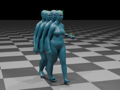
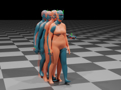
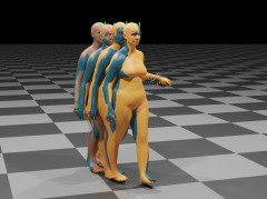
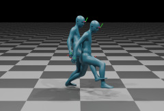
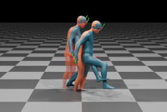
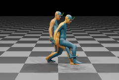
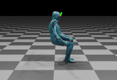
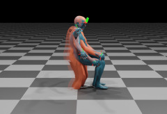
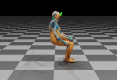
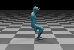
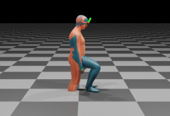
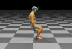
Figure A.3: Comparison of our learned fitter with a Levenberg-Marquardt based optimization method. Left to right: 1) Input HMD data and Ground-Truth mesh (blue), 2) LM solution (orange) overlayed on the GT, 3) our solution (yellow) overlayed on the GT. While the classic LM optimization successfully fits the input data, it still needs hand-crafted priors to prevent ground floor penetration. In contrast, our proposed fitter learns from the data to avoid such penetrations.

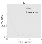
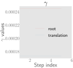
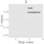
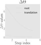
Figure A.4: Average norm for (left to right) 1) $\lVert\bm{g}_{n}\rVert_{2}$, 2) $\lVert\bm{\gamma}\rVert_{2}$, 3) $\lVert\bm{\lambda}\rVert_{2}$ and 4) $\lVert\Delta\bm{\Theta}_{n}\rVert_{2}$, computed across the test set, for the root rotation and translation. The learned optimizer slows down as it approaches a minimum of the target data term.

References

- [1] Adler, J., Öktem, O.: Solving ill-posed inverse problems using iterative deep neural networks. Inverse Problems 33(12), 124007 (2017)
- [2] Andrychowicz, M., Denil, M., Gómez, S., Hoffman, M.W., Pfau, D., Schaul, T., Shillingford, B., de Freitas, N.: Learning to learn by gradient descent by gradient descent. In: NeurIPS. vol. 29. Curran Associates, Inc. (2016), https://proceedings.neurips.cc/paper/2016/file/fb87582825f9d28a8d42c5e5e5e8b23d-Paper.pdf
- [3] Anguelov, D., Srinivasan, P., Koller, D., Thrun, S., Rodgers, J., Davis, J.: SCAPE: Shape Completion and Animation of People. ACM Transactions on Graphics 24(3), 408–416 (July 2005). https://doi.org/10.1145/1073204.1073207, https://doi.org/10.1145/1073204.1073207
- [4] Ba, J.L., Kiros, J.R., Hinton, G.E.: Layer normalization. arXiv preprint arXiv:1607.06450 (2016)
- [5] Baek, S., Kim, K.I., Kim, T.K.: Pushing the envelope for RGB-based dense 3D hand pose estimation via neural rendering. In: Computer Vision and Pattern Recognition (CVPR). pp. 1067–1076 (June 2019)
- [6] Barron, J.T.: A general and adaptive robust loss function. Computer Vision and Pattern Recognition (CVPR) pp. 4326–4334 (June 2019)
- [7] Biggs, B., Novotny, D., Ehrhardt, S., Joo, H., Graham, B., Vedaldi, A.: 3D Multi-bodies: Fitting Sets of Plausible 3D Human Models to Ambiguous Image Data. In: NeurIPS. vol. 33, pp. 20496–20507. Curran Associates, Inc. (2020), https://proceedings.neurips.cc/paper/2020/file/ebf99bb5df6533b6dd9180a59034698d-Paper.pdf
- [8] Blanz, V., Vetter, T.: A morphable model for the synthesis of 3D faces. In: ACM Transactions on Graphics (Proceedings of SIGGRAPH). pp. 187–194 (1999)
- [9] Bogo, F., Kanazawa, A., Lassner, C., Gehler, P., Romero, J., Black, M.J.: Keep it SMPL: Automatic estimation of 3D human pose and shape from a single image. In: European Conference on Computer Vision (ECCV). pp. 561–578. Lecture Notes in Computer Science, Springer International Publishing (October 2016)
- [10] Boukhayma, A., Bem, R.d., Torr, P.H.: 3D hand shape and pose from images in the wild. In: Computer Vision and Pattern Recognition (CVPR). pp. 10843–10852 (June 2019)
- [11] Cao, Z., Hidalgo, G., Simon, T., Wei, S.E., Sheikh, Y.: OpenPose: Realtime Multi-Person 2D Pose Estimation using Part Affinity Fields. Transactions on Pattern Analysis and Machine Intelligence (TPAMI) 43(1), 172–186 (2021)
- [12] Carnegie Mellon University: CMU MoCap Dataset, http://mocap.cs.cmu.edu
- [13] Cho, K., van Merriënboer, B., Gulcehre, C., Bahdanau, D., Bougares, F., Schwenk, H., Bengio, Y.: Learning phrase representations using RNN encoder–decoder for statistical machine translation. In: Proceedings of the 2014 Conference on Empirical Methods in Natural Language Processing (EMNLP). pp. 1724–1734. Association for Computational Linguistics, Doha, Qatar (Oct 2014). https://doi.org/10.3115/v1/D14-1179, https://aclanthology.org/D14-1179
- [14] Choi, H., Moon, G., Lee, K.M.: Beyond Static Features for Temporally Consistent 3D Human Pose and Shape from a Video. In: Computer Vision and Pattern Recognition (CVPR). pp. 1964–1973 (June 2021)
- [15] Choutas, V., Pavlakos, G., Bolkart, T., Tzionas, D., Black, M.J.: Monocular Expressive Body Regression through Body-Driven Attention. In: European Conference on Computer Vision (ECCV). pp. 20–40 (August 2020)
- [16] Clark, R., Bloesch, M., Czarnowski, J., Leutenegger, S., Davison, A.J.: Learning to Solve Nonlinear Least Squares for Monocular Stereo. In: European Conference on Computer Vision (ECCV). pp. 291–306 (September 2018)
- [17] Dehesa, J., Vidler, A., Padget, J., Lutteroth, C.: Grid-Functioned Neural Networks. In: ICML. Proceedings of Machine Learning Research, vol. 139, pp. 2559–2567. PMLR (July 2021), https://proceedings.mlr.press/v139/dehesa21a.html
- [18] Dittadi, A., Dziadzio, S., Cosker, D., Lundell, B., Cashman, T.J., Shotton, J.: Full-Body Motion From a Single Head-Mounted Device: Generating SMPL Poses From Partial Observations. In: International Conference on Computer Vision (ICCV). pp. 11687–11697 (October 2021)
- [19] Dong, Z., Song, J., Chen, X., Guo, C., Hilliges, O.: Shape-aware Multi-Person Pose Estimation from Multi-View Images. In: International Conference on Computer Vision (ICCV). pp. 11158–11168 (October 2021)
- [20] Duchi, J., Hazan, E., Singer, Y.: Adaptive Subgradient Methods for Online Learning and Stochastic Optimization. Journal of Machine Learning Research 12(7), 2121––2159 (2011)
- [21] Egger, B., Smith, W.A.P., Tewari, A., Wuhrer, S., Zollhoefer, M., Beeler, T., Bernard, F., Bolkart, T., Kortylewski, A., Romdhani, S., Theobalt, C., Blanz, V., Vetter, T.: 3D Morphable Face Models - Past, Present and Future. ACM Transactions on Graphics 39(5) (August 2020). https://doi.org/10.1145/3395208
- [22] Fan, T., Alwala, K.V., Xiang, D., Xu, W., Murphey, T., Mukadam, M.: Revitalizing Optimization for 3D Human Pose and Shape Estimation: A Sparse Constrained Formulation. In: International Conference on Computer Vision (ICCV). pp. 11457–11466 (October 2021)
- [23] Feng, Y., Choutas, V., Bolkart, T., Tzionas, D., Black, M.J.: Collaborative regression of expressive bodies using moderation. In: International Conference on 3D Vision (3DV). pp. 792–804 (2021)
- [24] Flynn, J., Broxton, M., Debevec, P., DuVall, M., Fyffe, G., Overbeck, R., Snavely, N., Tucker, R.: DeepView View Synthesis with Learned Gradient Descent. In: Computer Vision and Pattern Recognition (CVPR). pp. 2367–2376 (June 2019)
- [25] Glorot, X., Bengio, Y.: Understanding the difficulty of training deep feedforward neural networks. In: Proceedings of the Thirteenth International Conference on Artificial Intelligence and Statistics. pp. 249–256. JMLR Workshop and Conference Proceedings (2010)
- [26] Guzov, V., Mir, A., Sattler, T., Pons-Moll, G.: Human POSEitioning System (HPS): 3D Human Pose Estimation and Self-Localization in Large Scenes From Body-Mounted Sensors. In: Computer Vision and Pattern Recognition (CVPR). pp. 4318–4329 (June 2021)
- [27] Hassan, M., Choutas, V., Tzionas, D., Black, M.J.: Resolving 3D human pose ambiguities with 3D scene constraints. In: International Conference on Computer Vision (ICCV). pp. 2282–2292 (October 2019), https://prox.is.tue.mpg.de
- [28] Hasson, Y., Varol, G., Tzionas, D., Kalevatykh, I., Black, M.J., Laptev, I., Schmid, C.: Learning Joint Reconstruction of Hands and Manipulated Objects. In: Computer Vision and Pattern Recognition (CVPR). pp. 11807–11816 (June 2019)
- [29] He, K., Zhang, X., Ren, S., Sun, J.: Deep residual learning for image recognition. In: Computer Vision and Pattern Recognition (CVPR). pp. 770–778 (June 2016)
- [30] Hochreiter, S., Schmidhuber, J.: Long short-term memory. Neural computation 9(8), 1735–1780 (1997)
- [31] Holden, D., Komura, T., Saito, J.: Phase-Functioned Neural Networks for Character Control. ACM Transactions on Graphics 36(4) (July 2017). https://doi.org/10.1145/3072959.3073663, https://doi.org/10.1145/3072959.3073663
- [32] Igel, C., Toussaint, M., Weishui, W.: Rprop using the natural gradient. In: Trends and Applications in Constructive Approximation. pp. 259–272. Birkhäuser Basel, Basel (2005)
- [33] Ioffe, S., Szegedy, C.: Batch normalization: Accelerating deep network training by reducing internal covariate shift. In: ICLR. pp. 448–456. PMLR (2015)
- [34] Joo, H., Neverova, N., Vedaldi, A.: Exemplar Fine-Tuning for 3D Human Pose Fitting Towards In-the-Wild 3D Human Pose Estimation. In: International Conference on 3D Vision (3DV). pp. 42–52 (2021)
- [35] Joo, H., Simon, T., Sheikh, Y.: Total capture: A 3D deformation model for tracking faces, hands, and bodies. In: Computer Vision and Pattern Recognition (CVPR). pp. 8320–8329 (June 2018)
- [36] Kanazawa, A., Black, M.J., Jacobs, D.W., Malik, J.: End-to-end recovery of human shape and pose. In: Computer Vision and Pattern Recognition (CVPR). pp. 7122–7131 (June 2018)
- [37] Kaufmann, M., Zhao, Y., Tang, C., Tao, L., Twigg, C., Song, J., Wang, R., Hilliges, O.: EM-POSE: 3D Human Pose Estimation From Sparse Electromagnetic Trackers. In: International Conference on Computer Vision (ICCV). pp. 11510–11520 (October 2021)
- [38] Kingma, D.P., Ba, J.: Adam: A method for stochastic optimization. In: ICLR (2015), http://arxiv.org/abs/1412.6980
- [39] Kocabas, M., Athanasiou, N., Black, M.J.: VIBE: Video inference for human body pose and shape estimation. In: Computer Vision and Pattern Recognition (CVPR). pp. 5252–5262 (June 2020)
- [40] Kocabas, M., Huang, C.H.P., Hilliges, O., Black, M.J.: PARE: Part attention regressor for 3D human body estimation. In: International Conference on Computer Vision (ICCV). pp. 11127–11137 (October 2021)
- [41] Kokkinos, F., Kokkinos, I.: To The Point: Correspondence-driven monocular 3D category reconstruction. In: NeurIPS (2021), https://openreview.net/forum?id=AWMU04iXQ08
- [42] Kolotouros, N., Pavlakos, G., Black, M.J., Daniilidis, K.: Learning to reconstruct 3D human pose and shape via Model-Fitting in the loop. In: International Conference on Computer Vision (ICCV). pp. 2252–2261 (October 2019)
- [43] Kolotouros, N., Pavlakos, G., Jayaraman, D., Daniilidis, K.: Probabilistic modeling for human mesh recovery. In: International Conference on Computer Vision (ICCV). pp. 11585–11594 (October 2021)
- [44] Levenberg, K.: A method for the solution of certain non-linear problems in least squares. Quarterly of applied mathematics 2(2), 164–168 (1944)
- [45] Li, J., Xu, C., Chen, Z., Bian, S., Yang, L., Lu, C.: HybrIK: A Hybrid Analytical-Neural Inverse Kinematics Solution for 3D Human Pose and Shape Estimation. In: Computer Vision and Pattern Recognition (CVPR). pp. 3383–3393 (June 2021)
- [46] Loper, M., Mahmood, N., Romero, J., Pons-Moll, G., Black, M.J.: SMPL: A Skinned Multi-Person Linear Model. ACM Transactions on Graphics (Proceedings of SIGGRAPH Asia) 34(6), 248:1–248:16 (October 2015)
- [47] Lv, Z., Dellaert, F., Rehg, J.M., Geiger, A.: Taking a deeper look at the inverse compositional algorithm. In: Computer Vision and Pattern Recognition (CVPR). pp. 4581–4590 (June 2019)
- [48] Mahmood, N., Ghorbani, N., Troje, N.F., Pons-Moll, G., Black, M.J.: AMASS: Archive of motion capture as surface shapes. In: International Conference on Computer Vision (ICCV). pp. 5442–5451 (October 2019)
- [49] Mandery, C., Terlemez, O., Do, M., Vahrenkamp, N., Asfour, T.: The KIT whole-body human motion database. In: 2015 International Conference on Advanced Robotics (ICAR). pp. 329–336 (Jul 2015). https://doi.org/10.1109/ICAR.2015.7251476
- [50] von Marcard, T., Henschel, R., Black, M., Rosenhahn, B., Pons-Moll, G.: Recovering Accurate 3D Human Pose in The Wild Using IMUs and a Moving Camera. In: European Conference on Computer Vision (ECCV). pp. 614–631 (September 2018)
- [51] Marquardt, D.W.: An algorithm for least-squares estimation of nonlinear parameters. Journal of the society for Industrial and Applied Mathematics 11(2), 431–441 (1963)
- [52] Mueller, F., Davis, M., Bernard, F., Sotnychenko, O., Verschoor, M., Otaduy, M.A., Casas, D., Theobalt, C.: Real-time pose and shape reconstruction of two interacting hands with a single depth camera. ACM Transactions on Graphics 38(4) (July 2019). https://doi.org/10.1145/3306346.3322958, https://doi.org/10.1145/3306346.3322958
- [53] Müller, M., Röder, T., Clausen, M., Eberhardt, B., Krüger, B., Weber, A.: Documentation mocap database HDM05. Tech. Rep. CG-2007-2, Universität Bonn (Jun 2007)
- [54] Nair, V., Hinton, G.E.: Rectified linear units improve restricted boltzmann machines. In: ICML (2010)
- [55] Nocedal, J., Wright, S.J.: Numerical Optimization. Springer, New York, NY, USA, second edn. (2006)
- [56] Paszke, A., Gross, S., Massa, F., Lerer, A., Bradbury, J., Chanan, G., Killeen, T., Lin, Z., Gimelshein, N., Antiga, L., Desmaison, A., Kopf, A., Yang, E., DeVito, Z., Raison, M., Tejani, A., Chilamkurthy, S., Steiner, B., Fang, L., Bai, J., Chintala, S.: Pytorch: An imperative style, high-performance deep learning library. In: Advances in Neural Information Processing Systems 32, pp. 8024–8035. Curran Associates, Inc. (2019), http://papers.neurips.cc/paper/9015-pytorch-an-imperative-style-high-performance-deep-learning-library.pdf
- [57] Patel, P., Huang, C.H.P., Tesch, J., Hoffmann, D.T., Tripathi, S., Black, M.J.: AGORA: Avatars in geography optimized for regression analysis. In: Computer Vision and Pattern Recognition (CVPR). pp. 13463–13473 (June 2021)
- [58] Pavlakos, G., Choutas, V., Ghorbani, N., Bolkart, T., Osman, A.A.A., Tzionas, D., Black, M.J.: Expressive body capture: 3D hands, face, and body from a single image. In: Computer Vision and Pattern Recognition (CVPR). pp. 10975–10985 (June 2019)
- [59] Powell, M.J.D.: A hybrid method for nonlinear equations. In: Numerical Methods for Nonlinear Algebraic Equations. Gordon and Breach (1970)
- [60] Rempe, D., Birdal, T., Hertzmann, A., Yang, J., Sridhar, S., Guibas, L.J.: HuMoR: 3D Human Motion Model for Robust Pose Estimation. In: International Conference on Computer Vision (ICCV). pp. 11468–11479 (October 2021)
- [61] Romero, J., Tzionas, D., Black, M.J.: Embodied hands: Modeling and capturing hands and bodies together. ACM Transactions on Graphics (Proceedings of SIGGRAPH Asia) 36(6) (November 2017)
- [62] Rong, Y., Shiratori, T., Joo, H.: FrankMocap: A Monocular 3D Whole-Body Pose Estimation System via Regression and Integration. In: International Conference on Computer Vision Workshops (ICCVw) (October 2021)
- [63] Schmidhuber, J.: Learning to control fast-weight memories: An alternative to dynamic recurrent networks. Neural Computation 4(1), 131–139 (1992)
- [64] Schmidhuber, J.: A neural network that embeds its own meta-levels. In: IEEE International Conference on Neural Networks. pp. 407–412. IEEE (1993)
- [65] Seeber, M., Poranne, R., Polleyfeyes, M., Oswald, M.: RealisticHands: A Hybrid Model for 3D Hand Reconstruction. In: International Conference on 3D Vision (3DV). pp. 22–31 (December 2021)
- [66] Shen, J., Cashman, T.J., Ye, Q., Hutton, T., Sharp, T., Bogo, F., Fitzgibbon, A.W., Shotton, J.: The Phong Surface: Efficient 3D Model Fitting using Lifted Optimization. In: European Conference on Computer Vision (ECCV). pp. 687–703. Springer (August 2020)
- [67] Song, J., Chen, X., Hilliges, O.: Human Body Model Fitting by Learned Gradient Descent. In: European Conference on Computer Vision (ECCV). pp. 744–760 (August 2020)
- [68] Srivastava, R.K., Greff, K., Schmidhuber, J.: Training very deep networks. In: NeurIPS. vol. 28. Curran Associates, Inc. (2015), https://proceedings.neurips.cc/paper/2015/file/215a71a12769b056c3c32e7299f1c5ed-Paper.pdf
- [69] Taylor, J., Bordeaux, L., Cashman, T., Corish, B., Keskin, C., Sharp, T., Soto, E., Sweeney, D., Valentin, J., Luff, B., Topalian, A., Wood, E., Khamis, S., Kohli, P., Izadi, S., Banks, R., Fitzgibbon, A., Shotton, J.: Efficient and precise interactive hand tracking through joint, continuous optimization of pose and correspondences. ACM Transactions on Graphics 35(4) (July 2016). https://doi.org/10.1145/2897824.2925965, https://doi.org/10.1145/2897824.2925965
- [70] Thies, J., Zollhofer, M., Stamminger, M., Theobalt, C., Nießner, M.: Face2Face: Real-time Face Capture and Reenactment of RGB Videos. In: Computer Vision and Pattern Recognition (CVPR). pp. 2387–2395 (June 2016)
- [71] Tomè, D., Alldieck, T., Peluse, P., Pons-Moll, G., Agapito, L., Badino, H., la Torre, F.D.: SelfPose: 3D Egocentric Pose Estimation from a Headset Mounted Camera. Transactions on Pattern Analysis and Machine Intelligence (TPAMI) pp. 1–1 (2020). https://doi.org/10.1109/TPAMI.2020.3029700
- [72] Tome, D., Peluse, P., Agapito, L., Badino, H.: xR-EgoPose: Egocentric 3D Human Pose from an HMD Camera. In: International Conference on Computer Vision (ICCV). pp. 7728–7738 (October 2019)
- [73] Vogel, C., Pock, T.: A primal dual network for low-level vision problems. In: Pattern Recognition. pp. 189–202. Springer International Publishing, Cham (2017)
- [74] Wood, E., Baltrušaitis, T., Hewitt, C., Dziadzio, S., Johnson, M., Estellers, V., Cashman, T.J., Shotton, J.: Fake It Till You Make It: Face Analysis in the Wild Using Synthetic Data Alone. In: International Conference on Computer Vision (ICCV). pp. 3681–3691 (October 2021)
- [75] Xiang, D., Joo, H., Sheikh, Y.: Monocular Total Capture: Posing Face, Body, and Hands in the Wild. In: Computer Vision and Pattern Recognition (CVPR). pp. 10965–10974 (June 2019)
- [76] Xie, K., Wang, T., Iqbal, U., Guo, Y., Fidler, S., Shkurti, F.: Physics-Based Human Motion Estimation and Synthesis From Videos. In: International Conference on Computer Vision (ICCV). pp. 11532–11541 (October 2021)
- [77] Xiong, X., De la Torre, F.: Supervised descent method and its applications to face alignment. In: Computer Vision and Pattern Recognition (CVPR). pp. 532–539 (June 2013)
- [78] Xu, H., Bazavan, E.G., Zanfir, A., Freeman, W.T., Sukthankar, R., Sminchisescu, C.: GHUM & GHUML: Generative 3D human shape and articulated pose models. In: Computer Vision and Pattern Recognition (CVPR). pp. 6183–6192 (June 2020)
- [79] Yang, D., Kim, D., Lee, S.H.: LoBSTr: Real-time Lower-body Pose Prediction from Sparse Upper-body Tracking Signals. Computer Graphics Forum (2021). https://doi.org/10.1111/cgf.142631
- [80] Yuan, Y., Kitani, K.: Ego-Pose Estimation and Forecasting as Real-Time PD Control. In: International Conference on Computer Vision (ICCV). pp. 10082–10092 (October 2019)
- [81] Yuan, Y., Kitani, K.M.: 3D Ego-Pose Estimation via Imitation Learning. In: European Conference on Computer Vision (ECCV). pp. 763 – 778 (September 2018)
- [82] Yuan, Y., Wei, S.E., Simon, T., Kitani, K., Saragih, J.: SimPoE: Simulated Character Control for 3D Human Pose Estimation. In: Computer Vision and Pattern Recognition (CVPR). pp. 7159–7169 (June 2021)
- [83] Zach, C.: Robust bundle adjustment revisited. In: European Conference on Computer Vision (ECCV). pp. 772–787. Springer International Publishing, Cham (September 2014)
- [84] Zanfir, A., Bazavan, E.G., Zanfir, M., Freeman, W.T., Sukthankar, R., Sminchisescu, C.: Neural Descent for Visual 3D Human Pose and Shape. In: Computer Vision and Pattern Recognition (CVPR). pp. 14484–14493 (June 2021)
- [85] Zhang, H., Tian, Y., Zhou, X., Ouyang, W., Liu, Y., Wang, L., Sun, Z.: PyMAF: 3D human pose and shape regression with pyramidal mesh alignment feedback loop. In: International Conference on Computer Vision (ICCV). pp. 11446–11456 (October 2021)
- [86] Zhang, S., Zhang, Y., Bogo, F., Marc, P., Tang, S.: Learning Motion Priors for 4D Human Body Capture in 3D Scenes. In: International Conference on Computer Vision (ICCV). pp. 11343–11353 (October 2021)
- [87] Zhou, Y., Barnes, C., Lu, J., Yang, J., Li, H.: On the continuity of rotation representations in neural networks. In: Computer Vision and Pattern Recognition (CVPR). pp. 5738–5746 (June 2019)
- [88] Zollhöfer, M., Thies, J., Garrido, P., Bradley, D., Beeler, T., Pérez, P., Stamminger, M., Nießner, M., Theobalt, C.: State of the art on monocular 3D face reconstruction, tracking, and applications. In: Computer Graphics Forum. vol. 37, pp. 523–550. Wiley Online Library (2018)