Blended Diffusion for Text-driven Editing of Natural Images

Abstract

Natural language offers a highly intuitive interface for image editing. In this paper, we introduce the first solution for performing local (region-based) edits in generic natural images, based on a natural language description along with an ROI mask. We achieve our goal by leveraging and combining a pretrained language-image model (CLIP), to steer the edit towards a user-provided text prompt, with a denoising diffusion probabilistic model (DDPM) to generate natural-looking results. To seamlessly fuse the edited region with the unchanged parts of the image, we spatially blend noised versions of the input image with the local text-guided diffusion latent at a progression of noise levels. In addition, we show that adding augmentations to the diffusion process mitigates adversarial results. We compare against several baselines and related methods, both qualitatively and quantitatively, and show that our method outperforms these solutions in terms of overall realism, ability to preserve the background and matching the text. Finally, we show several text-driven editing applications, including adding a new object to an image, removing/replacing/altering existing objects, background replacement, and image extrapolation.

1 Introduction

It is said that “a picture is worth a thousand words”, but recent research indicates that only a few words are often sufficient to describe one. Recent works that leverage the tremendous progress in vision-language models and data-driven image generation have demonstrated that text-based interfaces for image creation and manipulation are now finally within reach [45, 12, 57, 52, 30, 63, 43, 31, 42, 24].

The most impressive results in text-driven image manipulation leverage the strong generative capabilities of modern GANs [20, 27, 28, 26, 6]. However, GAN-based approaches are typically limited to images from a restricted domain, on which the GAN was trained. Furthermore, in order to manipulate real images, they must be first inverted into the GAN’s latent space. Although many GAN inversion techniques have recently emerged [58, 1, 65, 2, 48, 3, 53], it was also shown that there is a trade-off between the reconstruction accuracy and the editability of the inverted images [53]. Restricting the image manipulation to a specific region in the image is another challenge for existing approaches [4].

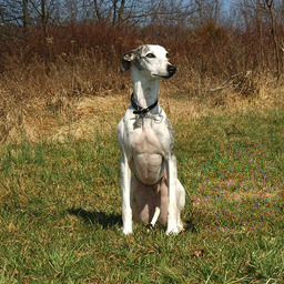
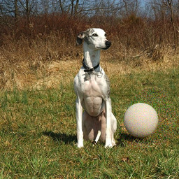
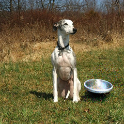
input+mask	no prompt	“white ball”	“bowl of water”
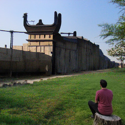
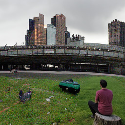
input+mask	“big mountain”	“big wall”	“New York City”

Figure 1: Text-driven object/background replacement: Given an input image and a mask, we modify the masked area according to a guiding text prompt, without affecting the unmasked regions.

In this work, we present the first approach for region-based editing of generic real-world natural images, using natural language text guidance. Specifically, we aim at a text-driven method that (1) can operate on real images, rather than generated ones, (2) is not restricted to a specific domain, such as human faces or bedrooms, (3) modifies only a user-specified region, while preserving the rest of the image, (4) yields globally coherent (seamless) editing results, and (5) capable of generating multiple results for the same input, because of the one-to-many nature of the task. Several examples of such edits are shown in Figure 1.

The demanding image editing scenario described above has not received much attention in the deep-learning era. In fact, the most closely related works are classical approaches, such as seamless cloning [41, 15] and image completion [22], none of which are text-driven. A more recent related work is zero-shot semantic image painting [4] in which arbitrary simple textual descriptions can be attributed to the desired location within an image. However, this method does not operate on real images (requirement 1), does not preserve the background of the image (requirement 3), and does not generate multiple outputs for the same input (requirement 5).

To achieve our goals, we utilize two off-the-shelf pre-trained models: Denoising Diffusion Probabilistic Models (DDPM) [25, 36, 11] and Contrastive Language-Image Pre-training (CLIP) [44]. DDPM is a class of probabilistic generative models that has recently been shown to surpass the image generation quality of state-of-the-art GANs [11]. We use DPPM as our generative backbone in order to ensure natural-looking results. The CLIP model is contrastively trained on a dataset of 400 million (image, text) pairs collected from the internet to learn a rich shared embedding space for images and text. We use CLIP in order to guide the manipulation to match the user-provided text prompt.

We show that a naïve combination of DDPM and CLIP to perform text-driven local editing fails to preserve the image background, and in many cases, leads to a less natural result. Instead, we propose a novel way to leverage the diffusion process, which blends the CLIP-guided diffusion latents with suitably noised versions of the input image, at each diffusion step. We show that this scheme produces natural-looking results that are coherent with the unaltered parts of the input. We further show that using extending augmentations at each step of the diffusion process reduces adversarial results. Our method utilizes pretrained DDPM and CLIP models, without requiring additional training.

In summary, our main contributions are: (1) We propose the first solution for general-purpose region-based image editing, using natural language guidance, applicable to real, diverse images. (2) Our background preservation technique guarantees that unaltered regions are perfectly preserved. (3) We demonstrate that a simple augmentation technique significantly reduces the risk of adversarial results, allowing us to use gradient-based diffusion guidance.

2 Related Work

Text-to-image synthesis.

Recently, we’ve witnessed significant advances in text-to-image generation. Initial RNN-based works [33] were quickly superseded by generative adversarial approaches, such as the seminal work by Reed et al. [47]. The latter was further improved by multi-stage architectures [60, 61] and an attention mechanism [59].

DALL-E [45] introduced a GAN-free two stage approach: first, a discrete VAE [55, 46] is trained to reduce the context for the transformer. Next, a transformer [56] is trained autoregressively to model the joint distribution over the text and image tokens.

Several recent projects [34, 9, 8] utilize a pretrained generative model [6, 14, 11] using a pretrained CLIP model [44] to steer the generated result towards the desired target description. These methods are mainly used to create abstract artworks from text descriptions and lack the ability to edit parts of a real image, while preserving the rest.

While text-to-image is a challenging and interesting task, in this work we focus on text-driven image manipulation, where edits are restricted to a user-specified region.

Text-driven image manipulation.

Several recent works utilize CLIP in order to manipulate real images. StyleCLIP [40] use pretrained StyleGAN2 [28] and CLIP models to modify images based on text prompts. To manipulate real images (rather than generated ones), they must first be encoded to the latent space [53]. This approach cannot handle generic real images, and is restricted to domains for which high-quality generators are available. In addition, StyleCLIP operates on images in a global fashion, without providing spatial control over which areas should change.

More closely related to ours is the work of Bau et al. [4], where arbitrary simple textual descriptions can be attributed to a desired location within an image. Their GAN-based approach has several limitations: (1) although they attempt to preserve the background, it may still change, as can be seen in Figure 5; (2) their solution is mainly demonstrated in the restricted domain of bedrooms, and mainly for color and texture editing tasks. A few examples of general images are shown, but the results are less natural or lack background preservation (see Figure 5). (3) Their model is able to operate only on generated images and is not applicable out-of-the-box to arbitrary natural images. GAN-inversion techniques [58, 1, 65, 2, 48, 3, 53] can be used to edit real images, but it was shown [53] that there is a trade-off between the edibility and the distortion of the reconstructed image.

Concurrently with our work, Liu et al. [32] and Kim et al. [29] propose ways to utilize a diffusion model in order to perform global text-guided image manipulations. In addition, GLIDE [35] is a concurrent work that utilizes the diffusion model for text-to-image synthesis, as well as local image editing using text guidance. In order to do so, they train a designated diffusion model for these tasks.

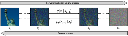
Figure 2: Denoising diffusion. Starting from a sample $x_{0}$, a forward Markovian noising process produces a series of noisy images by gradually adding Gaussian noise $q(x_{t}|x_{t-1})$, until obtaining a nearly isotropic Gaussian noise sample $x_{T}$. The reverse process transforms a Gaussian noise sample $x_{T}$ into $x_{0}$ by repeated denoising using a learned posterior $p_{\theta}(x_{t-1}|x_{t})$.

3 Denoising Diffusion Probabilistic Models

Denoising diffusion probabilistic models (DDPMs) learn to invert a parameterized Markovian image noising process. Starting from isotropic Gaussian noise samples, they transform them to samples from a training distribution, gradually removing the noise by an iterative diffusion process (Fig. 2). DDPMs have recently been shown to generate high-quality images [25, 36, 11]. Below, we provide a brief overview of DDPMs, for more details please refer to [49, 25, 36]. We follow the formulations and notations in [36].

Given a data distribution $x_{0}\sim q(x_{0})$, a forward noising process produces a series of latents $x_{1},...,x_{T}$ by adding Gaussian noise with variance $\beta_{t}\in(0,1)$ at time $t$:

$$\begin{split}q(x_{1},...,x_{T}|x_{0})&=\prod_{t=1}^{T}q(x_{t}|x_{t-1})\\ q(x_{t}|x_{t-1})&=\mathcal{N}(\sqrt{1-\beta_{t}}x_{t-1},\beta_{t}\mathbf{I})\end{split}$$ (1)

When $T$ is large enough, the last latent $x_{T}$ is nearly an isotropic Gaussian distribution.

An important property of the forward noising process is that any step $x_{t}$ may be sampled directly from $x_{0}$, without the need to generate the intermediate steps,

$$\begin{split}q(x_{t}|x_{0})&=\mathcal{N}(\sqrt{\bar{\alpha}_{t}}x_{0},(1-\bar{\alpha}_{t})\mathbf{I})\\ x_{t}&=\sqrt{\bar{\alpha}_{t}}x_{0}+\sqrt{1-\bar{\alpha}_{t}}\epsilon,\end{split}$$ (2)

where $\epsilon\sim\mathcal{N}(0,\mathbf{I})$, $\alpha_{t}=1-\beta_{t}$ and $\bar{\alpha}_{t}=\prod_{s=0}^{t}\alpha_{s}$.

To draw a new sample from the distribution $q(x_{0})$ the Markovian process is reversed. That is, starting from a Gaussian noise sample, $x_{T}\sim\mathcal{N}(0,\mathbf{I})$, a reverse sequence is generated by sampling the posteriors $q(x_{t-1}|x_{t})$, which were shown to also be Gaussian distributions [17, 49].

However, $q(x_{t-1}|x_{t})$ is unknown, as it depends on the unknown data distribution $q(x_{0})$. In order to approximate this function, a deep neural network $p_{\theta}$ is trained to predict the mean and the covariance of $x_{t-1}$ given $x_{t}$ as input. Then $x_{t-1}$ may be sampled from the normal distribution defined by these parameters,

$$p_{\theta}(x_{t-1}|x_{t})=\mathcal{N}(\mu_{\theta}(x_{t},t),\Sigma_{\theta}(x_{t},t)).$$ (3)

Rather than inferring $\mu_{\theta}(x_{t},t)$ directly, Ho et al. [25] propose to predict the noise $\epsilon_{\theta}(x_{t},t)$ that was added to $x_{0}$ in order to obtain $x_{t}$, according to Equation 2. Then $\mu_{\theta}(x_{t},t)$ may be derived using Bayes’ theorem:

$$\mu_{\theta}(x_{t},t)=\frac{1}{\sqrt{\alpha_{t}}}\left(x_{t}-\frac{\beta_{t}}{\sqrt{1-\bar{\alpha}_{t}}}\epsilon_{\theta}(x_{t},t)\right)$$ (4)

For more details please see [25].

Ho et al. [25] kept $\Sigma_{\theta}(x_{t},t)$ constant, but it was later shown [36] that it is better to learn it by a neural network that interpolates between the upper and lower bounds for the fixed covariance proposed by Ho et al.

Dhariwal and Nichol [11] show that diffusion models can achieve image sample quality superior to the current state-of-the-art generative models. They improved the results of [25], in terms of FID score [23], by tuning the network architecture and by incorporating guidance using a classifier pretrained on noisy images. For more details please see the supplementary and the original paper [11].

4 Method

Given an image $x$, a guiding text prompt $d$ and a binary mask $m$ that marks the region of interest in the image, our goal is to produce a modified image $\widehat{x}$, s.t. the content $\widehat{x}\odot m$ is consistent with the text description $d$, while the complementary area remains as close as possible to the source image, i.e., $x\odot(1-m)\approx\widehat{x}\odot(1-m)$, where $\odot$ is element-wise multiplication. Furthermore, the transition between the two areas of $\widehat{x}$ should ideally appear seamless.

In Section 4.1 we start by adapting the DDPM approach described above to incorporate local text-driven editing by adding a guiding loss comprised of a masked CLIP loss and a background preservation term. The resulting method still falls short of satisfying our requirements, and we proceed to present a new text-driven blended diffusion method in Section 4.2, which guarantees background preservation and improves the coherence of the edited result. Section 4.2.2 introduces an augmentation technique that we employ in order to avoid adversarial results.

4.1 Local CLIP-guided diffusion

Dhariwal and Nichol [11] use a classifier pretrained on noisy images to guide generation towards a target class. Similarly, a pretrained CLIP model may be used to guide diffusion towards a target prompt. Since CLIP is trained on clean images (and retraining it on noisy images is impractical), we need a way of estimating a clean image $x_{0}$ from each noisy latent $x_{t}$ during the denoising diffusion process. Recall that the process estimates at each step the noise $\epsilon_{\theta}(x_{t},t)$ that was added to $x_{0}$ to obtain $x_{t}$. Thus, $x_{0}$ may be obtained from $\epsilon_{\theta}(x_{t},t)$ via Equation 2:

$$\widehat{x}_{0}=\frac{x_{t}}{\sqrt{\bar{\alpha}_{t}}}-\frac{\sqrt{1-\bar{\alpha}_{t}}\epsilon_{\theta}(x_{t},t)}{\sqrt{\bar{\alpha}_{t}}}$$ (5)

Now, a CLIP-based loss $\mathcal{D}_{\mathit{CLIP}}$ may be defined as the cosine distance between the CLIP embedding of the text prompt and the embedding of the estimated clean image $\widehat{x}_{0}$:

$$\mathcal{D}_{\mathit{CLIP}}(x,d,m)=~{}D_{c}(\mathit{CLIP}_{\mathit{img}}(x\odot m),\mathit{CLIP}_{\mathit{txt}}(d))$$ (6)

where $D_{c}$ denotes cosine distance. A similar approach is used in CLIP-guided diffusion [8], where a linear combination of $x_{t}$ and $\widehat{x}_{0}$ is used to provide global guidance for the diffusion. The guidance can be made local, by considering only the gradients of $\mathcal{D}_{\mathit{CLIP}}$ under the input mask. In this manner, we effectively adapt CLIP-guided diffusion [8] to the local (region-based) editing setting.

The above process starts from an isotropic Gaussian noise and has no background constraints. Thus, although $\mathcal{D}_{\mathit{CLIP}}$ is evaluated inside the masked region, it affects the entire image. In order to steer the surrounding region towards the input image, a background preservation loss $\mathcal{D}_{bg}$ is added to guide the diffusion outside the mask:

$$\begin{split}\mathcal{D}_{bg}(x_{1},x_{2},m)=d(x_{1}\odot(1-m),x_{2}\odot(1-m))\\ d(x_{1},x_{2})=\frac{1}{2}(\textit{MSE}(x_{1},x_{2})+\textit{LPIPS}(x_{1},x_{2}))\end{split}$$ (7)

where MSE is the $L_{2}$ norm of the pixel-wise difference between the images, and LPIPS is the Learned Perceptual Image Patch Similarity metric [62].

The diffusion guidance loss is thus set to the weighted sum $\mathcal{D}_{\mathit{CLIP}}(\widehat{x}_{0},d,m)+\lambda\mathcal{D}_{bg}(x,\widehat{x}_{0},m)$, and the resulting method is summarized in Algorithm 1.

Algorithm 1 Local CLIP-guided diffusion, given a diffusion model $(\mu_{\theta}(x_{t}),\Sigma_{\theta}(x_{t}))$ and $\mathit{CLIP}$ model

  Input: source image $x$, target text description $d$, input mask $m$, diffusion steps $k$, background preservation coefficient $\lambda$

  Output: edited image $\widehat{x}$ that differs from input image $x$ inside area $m$ according to text description $d$

  $x_{k}\sim\mathcal{N}(\sqrt{\bar{\alpha}_{k}}x_{0},(1-\bar{\alpha}_{k})\mathbf{I})$

  for all $t$ from $k$ to 1 do

     $\mu,\Sigma\leftarrow\mu_{\theta}(x_{t}),\Sigma_{\theta}(x_{t})$

     $\widehat{x}_{0}\leftarrow\frac{x_{t}}{\sqrt{\bar{\alpha}_{t}}}-\frac{\sqrt{1-\bar{\alpha}_{t}}\epsilon_{\theta}(x_{t},t)}{\sqrt{\bar{\alpha}_{t}}}$

     $\widehat{x}_{0,{\textit{aug}}}\leftarrow{\textit{ExtendingAugmentations}(\widehat{x}_{0},N)}$

     $\mathcal{L}\leftarrow\mathcal{D}_{\textit{CLIP}}(\widehat{x}_{0,{\textit{aug}}},d,m)+\lambda\mathcal{D}_{\textit{bg}}(x,\widehat{x}_{0,{\textit{aug}}},m)$

     $x_{t-1}\sim\mathcal{N}(\mu+\Sigma\nabla_{\widehat{x}_{0}}{\mathcal{L}},\Sigma)$

  end for

  return  $x_{0}$

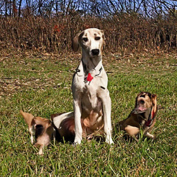
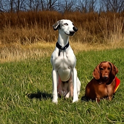
Input + mask	$\lambda=100$	$\lambda=1000$	$\lambda=10000$

Figure 3: Effect of $\lambda$ in local CLIP-guided diffusion. Given an input image with a mask, and the prompt “a dog”: with $\lambda$ set too low ($\lambda=100$), the entire image changes completely, while if $\lambda$ is too high ($\lambda=10000$), the model fails to change the foreground (and the background preservation is not perfect). Using an intermediate value ($\lambda=1000$) the model changes the foreground while resembling the original background (zoom for more details).

In practice, we have found that an inherent trade-off exists between the two guidance terms above, as demonstrated in Figure 3. Note that even in the intermediate case of $\lambda=1000$ the result is far from perfect: the background is only roughly preserved and the foreground is severely limited. We overcome this issue in the next section.

Algorithm 2 Text-driven blended diffusion: given a diffusion model $(\mu_{\theta}(x_{t}),\Sigma_{\theta}(x_{t}))$, and $\mathit{CLIP}$ model

  Input: source image $x$, target text description $d$, input mask $m$, diffusion steps $k$, number of extending augmentations $N$

  Output: edited image $\widehat{x}$ that differs from input image $x$ inside area $m$ according to text description $d$

  $x_{k}\sim\mathcal{N}(\sqrt{\bar{\alpha}_{k}}x_{0},(1-\bar{\alpha}_{k})\mathbf{I})$

  for all $t$ from $k$ to 0 do

     $\mu,\Sigma\leftarrow\mu_{\theta}(x_{t}),\Sigma_{\theta}(x_{t})$

     $\widehat{x}_{0}\leftarrow\frac{x_{t}}{\sqrt{\bar{\alpha}_{t}}}-\frac{\sqrt{1-\bar{\alpha}_{t}}\epsilon_{\theta}(x_{t},t)}{\sqrt{\bar{\alpha}_{t}}}$

     $\widehat{x}_{0,{\textit{aug}}}\leftarrow{\textit{ExtendingAugmentations}(\widehat{x}_{0},N)}$

     $\nabla_{\textit{text}}\leftarrow\frac{1}{N}\sum_{i=1}^{N}\nabla_{\widehat{x}_{0,{\textit{aug}}}}\mathcal{D}_{\textit{CLIP}}(\widehat{x}_{0,{\textit{aug}}},d,m)$

     $x_{\textit{fg}}\sim\mathcal{N}(\mu+\Sigma\nabla_{\textit{text}},\Sigma)$

     $x_{\textit{bg}}\sim\mathcal{N}(\sqrt{\bar{\alpha}_{t}}x_{0},(1-\bar{\alpha}_{t})\mathbf{I})$

     $x_{t-1}\leftarrow x_{\textit{fg}}\odot m+x_{\textit{bg}}\odot(1-m)$

  end for

  return  $x_{-1}$

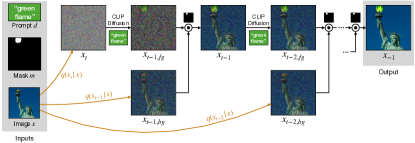
Figure 4: Text-driven blended diffusion. Given input image $x$, input mask $m$, and a text prompt $d$, we leverage the diffusion process to edit the image locally and coherently. We denote with $\odot$ the element-wise blending of two images using the input mask $m$.

4.2 Text-driven blended diffusion

The forward noising process implicitly defines a progression of image manifolds, where each manifold consists of noisier images. Each step of the reverse, denoising diffusion process, projects a noisy image onto the next, less noisy, manifold. To create a seamless result where the masked region complies with a guiding prompt, while the rest of the image is identical to the original input, we spatially blend each of the noisy images progressively generated by the CLIP-guided process with the corresponding noisy version of the input image. Our key insight is that, while in each step along the way, the result of blending the two noisy images is not guaranteed to be coherent, the denoising diffusion step that follows each blend, restores coherence by projecting onto the next manifold. This process is depicted in Figure 4 and summarized in Algorithm 2.

4.2.1 Background preserving blending

A naïve way to preserve the background is to let the CLIP-guided diffusion process generate an image $\widehat{x}$ without any background constraints (by setting $\lambda=0$ in Algorithm 1). Next, replace the generated background with the original one, taken from the input image: $\widehat{x}\odot m+x\odot(1-m)$. The obvious problem is that combining the two images in this manner fails to produce a coherent, seamless result. See the supplementary for an example.

In their pioneering work, Burt and Adelson [7] show that two images can be blended smoothly by separately blending each level of their Laplacian pyramids. Inspired by this technique, we propose to perform the blending at different noise levels along the diffusion process. Our key hypothesis is that at each step during the diffusion process, a noisy latent is projected onto a manifold of natural images noised to a certain level. While blending two noisy images (from the same level) yields a result that likely lies outside the manifold, the next diffusion step projects the result onto the next level manifold, thus ameliorating the incoherence.

Thus, at each stage, starting from a latent $x_{t}$, we perform a single CLIP-guided diffusion step, that denoises the latent in a direction dependent on the text prompt, yielding a latent denoted $x_{t-1,\textit{fg}}$. In addition, we obtain a noised version of the background $x_{t-1,\textit{bg}}$ from the input image using Equation 2. The two latents are now blended using the mask: $x_{t-1}=x_{t-1,\mathit{fg}}\odot m+x_{t-1,\mathit{bg}}\odot(1-m)$, and the process is repeated (see Figure 4 and Algorithm 2).

In the final step, the entire region outside the mask is replaced with the corresponding region from the input image, thus strictly preserving the background.

4.2.2 Extending augmentations

Adversarial examples [51, 21] is a well known phenomenon that may occur when optimizing an image directly on its pixel values. For example, a classifier can be easily fooled to classify an image incorrectly by slightly altering its pixels in the direction of their gradients with respect to some wrong class. Adding such adversarial noise will not be perceived by a human, but the classification will be wrong.

Similarly, gradual changes of pixel values by CLIP-guided diffusion, might result in reducing the CLIP loss without creating the desired high-level semantic change in the image. We find that this phenomenon frequently occurs in practice. Bau et al. [4] also experienced this issue and addressed it using a non-gradient method that is based on evolution strategy.

We hypothesized that this problem can be mitigated by performing several augmentations on the intermediate result estimated at each diffusion step, and calculating the gradients using CLIP on each of the augmentations separately. This way, in order to “fool” CLIP, the manipulation must do so on all the augmentations, which is harder to achieve without a high-level change in the image. Indeed, we find that a simple augmentation technique mitigates this problem: given the current estimated result $\widehat{x}_{0}$, instead of taking the gradients of the CLIP loss directly, we compute them with respect to several projectively transformed copies of this image. These gradients are then averaged together. We term this strategy as “extending augmentation”. The effect of these augmentations is studied in Section 5.2. We’ve added extending augmentations to our method (Algorithm 2) as well as to the Local CLIP GD baseline (Algorithm 1) for all the comparisons in this paper.

4.2.3 Result ranking

Algorithm 2 can generate multiple outputs for the same input; this is a desirable feature because our task is one-to-many by its nature. Similarly to [46, 45], we found it beneficial to generate multiple predictions, rank them and choose those with the higher scores. For the ranking, we utilize the CLIP model using the same $\mathcal{D}_{\mathit{CLIP}}$ from Equation 6 on the final results, without the extending augmentations.

AAInput + mask
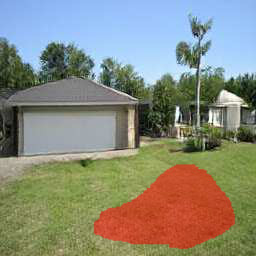
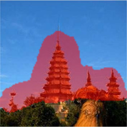
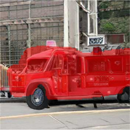
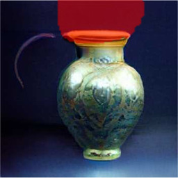
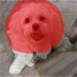
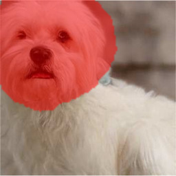
AAAAA (1)
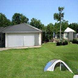
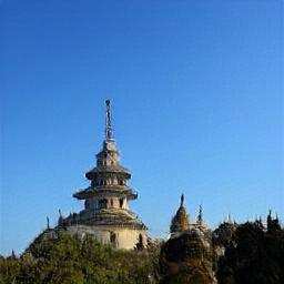
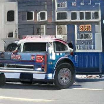
AAAAA(2)
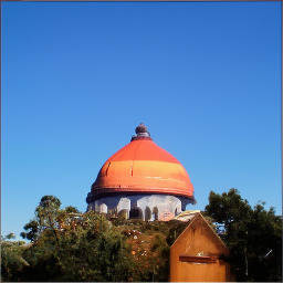
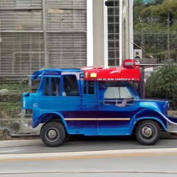
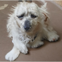
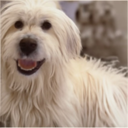
AAAAA(3)
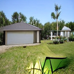
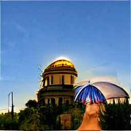
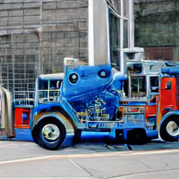
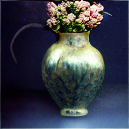
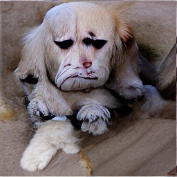
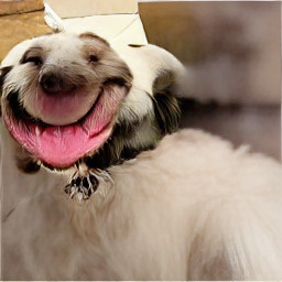
AAAAAOur
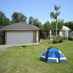
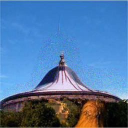
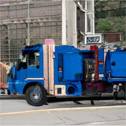
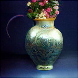
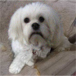
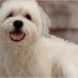
“A photo of a	“A photo of a	“A photo of a	“A photo of a	“A photo of a	“A photo of a
camping tent”	magnificent dome”	blue firetruck”	bouquet of flowers”	sad dog”	happy dog”

Figure 5: Comparison using examples from Paint By Word [4]. We use the GAN-generated input images, and user-provided masks and text prompts from Bau et al. [4], as well as their results (1). In the next two rows, we show results of two other baselines: (2) Local CLIP GD [8] and (3) PaintByWord++ [9, 4]. Our results (bottom row) exhibit more realistic objects. Moreover, our method perfectly preserves the background region of the input image, while other methods change it.

5 Results

We begin by comparing our method to previous methods and baselines both qualitatively and quantitatively. Next, we demonstrate the effect of our use of extending augmentations. Finally, we demonstrate several applications enabled by our method.

5.1 Comparisons

AA Input + mask
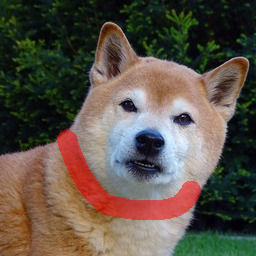
AAAAA(1)
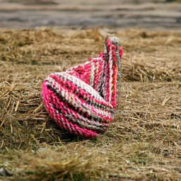
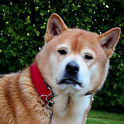
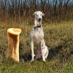
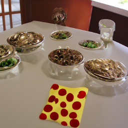
AAAAAA(2)
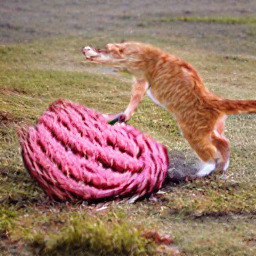
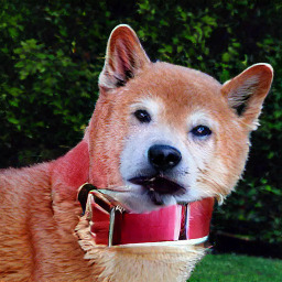
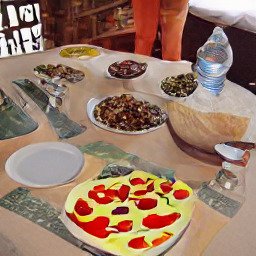
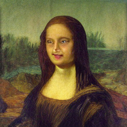
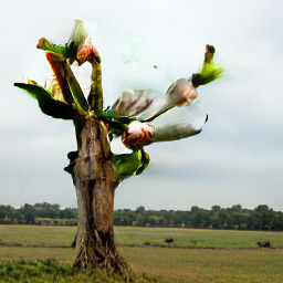
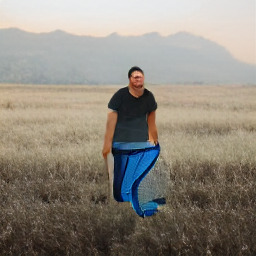
AAAAA Our
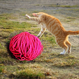
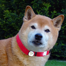
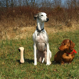
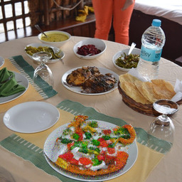
	“pink yarn ball”	“red dog collar”	“dog bone”	“pizza”	“golden necklace”	“blooming tree”	“tie with black	“blue short pants”
							and yellow stripes”

Figure 6: Comparison to baselines on real images: A comparison with (1) Local CLIP-guided diffusion [8] and (2) PaintByWord++ [4, 9]. Both baselines fail to preserve the background and produce results that are less natural/coherent, in contrast to the results of our method.

AAA“sausages”
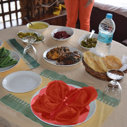
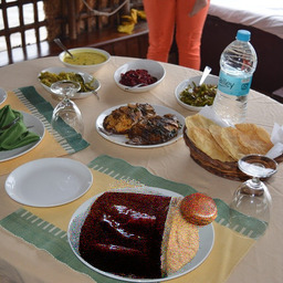
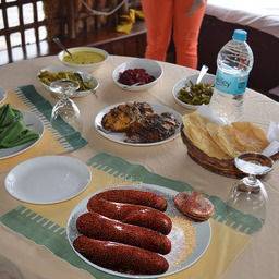
AA“huge avocado”
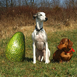
	Input + mask	(1)	(2)

Figure 7: Extending augmentations ablation: Using the same random seed and inputs, we compared the generated results (1) without extending augmentations and (2) with them. The augmentations make the resulting images more natural and coherent with the background. See supplementary material for more examples.

In Figure 5 we compare the text-driven edits performed by our method to those performed using (1) PaintByWord [4]; (2) local CLIP-guided diffusion, as described in Algorithm 1, with $\lambda=1000$; and (3) VQGAN-CLIP + Paint By Word [9, 4]. For the latter, we adapt VQGAN-CLIP [9] to support masks using the same $\mathcal{D}_{\mathit{CLIP}}$ loss from Equation 6. In addition, we find that results can be improved by optimizing only part of the VQGAN [14] latent space that corresponds to the edited area, similarly to the process in Bau et al. [4]. Because VQGAN includes a pretrained decoder, we can easily use this method on real images. We denote this method PaintByWord++.

Since the implementation of Bau et al. [4] is not currently available, we perform this comparison using the examples included in their paper. Note that since PaintByWord operates only on GAN-generated images, all the input images in this comparison are synthetic and somewhat unnatural. In order to achieve better results on places, Bau et al. [4] used two different models: one that is trained on MIT Places [64] and the other on ImageNet [10]. In contrast, our method can operate on real images and uses a single DPPM model that was trained on ImageNet.

The results shown in Figure 5 demonstrate that although PaintByWord and the other two baselines all encourage background preservation, the background is not always preserved and some global changes occur in almost all cases. Furthermore, in each of the rows (1)–(3) there are some results that appear unrealistic. In contrast, our method preserves the background perfectly, and the edits appear natural and coherent with the surrounding background.

Method Realism $\uparrow$ Background $\uparrow$ Text match $\uparrow$ PaintByWord [4] $3.31\pm 1.38$ $3.25\pm 1.33$ $3.14\pm 1.31$ Local CLIP GD [8] $3.50\pm 1.19$ $3.11\pm 1.24$ $3.86\pm 1.32$ PaintByWord++ [9, 4] $1.94\pm 1.36$ $3.37\pm 1.30$ $3.01\pm 1.38$ Ours $\bm{3.93\pm 1.08}$ $\bm{4.73\pm 0.61}$ $\bm{4.63\pm 0.77}$

Table 1: User study results: Participants were presented with the inputs and results shown in Figure 5 and were asked to rate each result on a Likert scale of 1-5 according to the following criteria: overall result realism, background preservation, and correspondence between the text prompt and the outcome. The mean and standard deviation are shown for each method and criterion.

In order to obtain quantitative results, we conducted a preliminary user study comparing between the different results shown in Figure 5. Participants were asked to rate each result in terms of realism, background preservation, and correspondence to the text prompt. Table 1 shows that our method outperforms the three baselines in all of these aspects. Please see the supplementary for more details.

In Figure 6 we further compare our method to local CLIP-guided diffusion and PaintByWord++, this time using real images as input. Again, the results demonstrate the inability of the baseline methods to preserve the background, and exhibit lack of coherence between the edited region and its surroundings, in contrast to the results of our method.

5.2 Ablation of extending augmentations

In order to assess the importance of the extending augmentation technique described Section 4.2.2, we disable the extending augmentations completely from our method (Algorithm 2). Figure 7 demonstrates the importance of the augmentations: the same random seed is used in two runs, one with and the other without augmentations. We can see that the images generated with the use of augmentations are more visually plausible and are more coherent than the ones generated without the augmentations.

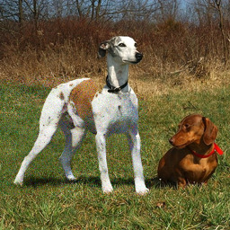
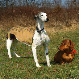
Input + mask	Result 1	Result 2	Result 3

Figure 8: Multiple outcomes: Given the same guiding text (top row: “a dog”, bottom row: “body of a standing dog”) our method generates multiple plausible results.

5.3 Applications

Our method is applicable to generic real-world images and may be used for a variety of applications. Below we demonstrate a few.

Text-driven object editing: we are able to add, remove or alter any of the existing objects in an image. Figure 8 demonstrates the ability to add a new object to an image. Note that the method is able to generate a variety of plausible outcomes. Rather than completely replacing an object, only a part of it may be replaced, guided by a text prompt, as shown in the bottom row of Figure 8. Figure 1 demonstrates the ability to remove an object or replace it with a new one. Removal is achieved by not providing any text prompt, and it is equivalent to traditional image inpainting, where no text or other guidance is involved.

Background replacement: rather than editing the foreground object, it is also possible to replace the background using text guidance, as demonstrated in Figure 1. Additional examples for foreground and background editing are included in supplementary results.

Scribble-guided editing: Due to the noising process of diffusion models, another image, or a user-provided scribble, may be used as a guide. For example, the user may scribble a rough shape on a background image, provide a mask (covering the scribble) to indicate the area that is allowed to change, as well as a text prompt. Our method will transform the scribble into a natural object while attempting to match the prompt, as demonstrated in Figure 9.

Original image	Input scribble	Result 1	Result 2

Figure 9: Scribble-guided editing: Users scribble a rough shape of the object they want to insert, mark the edited area, and provide a guiding text - “blanket”. The model uses the scribble as a general shape and color reference, transforming it to match the guiding text. Note that the scribble patterns can also change.

Text-guided image extrapolation is the ability to extend an image beyond its boundaries, guided by a textual description, s.t. the resulting change is gradual. Figure 10 demonstrates this ability: the user provides an image and two text prompts, each prompt is used to extrapolate the image in one direction. The resulting image can be arbitrarily wide (and mix multiple prompts). More details are provided in the supplementary material.

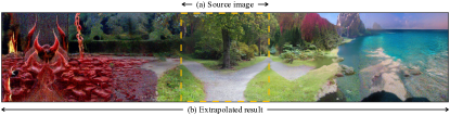
Figure 10: Text-guided image extrapolation: The user provides an input image and two text descriptions: “hell” and “heaven”. The model extrapolates the image to the left using the “hell” prompt and to the right using the “heaven” prompt.

6 Limitations and Future Work

The main limitation of our work is its inference time. Because of the sequential nature of DDPMs, generating a single image takes about 30 seconds on a modern GPU as described in the supplementary. In addition, we generate several samples and choose the top-ranked ones, as described in Section 4.2.3. This limits the applicability of our method for real-time applications and weak end-user devices (e.g. mobile devices). Further research in accelerating diffusion sampling is needed to address this problem.

In addition, the ranking method presented in Section 4.2.3 is not perfect because it takes into account only the edited area without the entire context of the image. So, bad results that contain only part of the desired object, may still get a high score, as demonstrated in Figure 11 (1). A better ranking system will enable our method to produce more compelling and coherent results.

Furthermore, because our model is based on CLIP, it inherits its weaknesses and biases. It was shown [19] that CLIP is susceptible to typographic attacks - exploiting the model’s ability to read text robustly, they found that even photographs of hand-written text can often fool the model. Figure 11 (2) demonstrates that this phenomenon can occur even when generating images: instead of generating an image of a “rubber toy” our method generates a sign with the word “rubber”.

Input + mask	(1)	(2)	(3)

Figure 11: Failure cases: Examples of failure cases given source image, mask and description “rubber toy”: (1) partial object — ranking by the edited area only may cause partial object to get a high score, (2) typographic bias — the model can generate a sign with the word “rubber” on it, (3) missing object and unnatural shadows — sometimes the method adds a shadow that is not coherent with the scene and does not correspond to the text.

One avenue for further research is training a version of CLIP that is agnostic to Gaussian noise. This may be done by training a version of CLIP that gets as an input a noisy image, a noise level, and the description text, and embeds the image and the text to a shared embedding space using contrastive loss. The noising process during training should be the same as in Equation 2.

Yet another avenue for research is extending our problem to other modalities such as a general-purpose text editor for 3D objects or videos.

7 Societal Impact

Photo manipulations are almost as old as the photo creation process itself [16]. Such manipulations can be used for art, entertainment, aesthetics, storytelling, and other legitimate use cases, but at the same time can also be used to tell lies via photos, for bullying, harassment, extortion, and may have psychological consequences [18]. Indeed, our method can be used for all of the above. For example, it can be misused to add credibility to fake news, which is a growing concern in the current media climate. It may also erode trust in photographic evidence and allow real events and real evidence to be brushed off as fake [5].

While our work does not enable anything that was out of reach for professional image editors, it certainly adds to the ease-of-use of the manipulation process, thus allowing users with limited technical capabilities to manipulate photos. We are passionate about our research, not only due to the legitimate use-cases, but also because we believe such research must be conducted openly in academia and not kept secret. We will provide our code for the benefit of the academic community, and we are actively working on the complement of this work: image and video forensic methods.

8 Conclusions

We introduced a novel solution to the problem of text-driven editing of natural images and demonstrated its superiority over the baselines. We believe that editing natural images using free text is a highly intuitive interaction, that will be further developed to a level which will make it an indispensable tool in the arsenal of every content creator.

Acknowledgments This work was supported in part by Lightricks Ltd and by the Israel Science Foundation (grants No. 2492/20 and 1574/21).

Appendix A Additional Examples

In this section we provide additional examples of the applications and the failure cases that were mentioned in the main paper. In addition, we show that our method naturally supports an iterative editing process. Lastly, we demonstrate the naïve blending approach (main paper, Section 4.2.1).

A.1 Applications — Additional Examples

We provide additional examples for the applications mentioned in the paper: Figures 12, 13 and 14 demonstrate the ability of our method to add new objects to an existing image, where Figures 12 and 13 show that different results can be obtained for the same text prompt, while Figure 14 shows results obtained using a variety of prompts. Figure 15 demonstrates the ability to remove or replace objects in an exiting image, while Figure 16 demonstrates the ability to alter an existing object in an image. Figures 17 and 18 demonstrate the ability to replace the background of an image. Figure 19 demonstrates more examples of scribble-guided editing, and Figure 20 demonstrates text-guided image extrapolation.

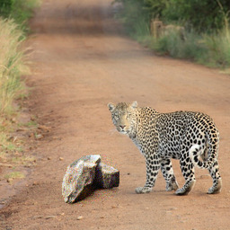
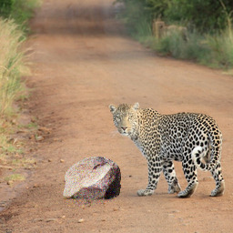
Input image	Image mask	Result 1	Result 2	Result 3	Result 4
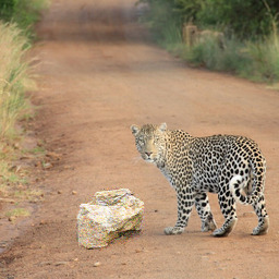
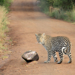
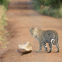
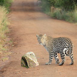
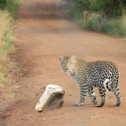
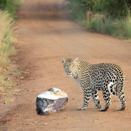
Result 5	Result 6	Result 7	Result 8	Result 9	Result 10

Figure 12: Adding a new object (multiple results for the same input): Given the input image, mask and text description “rock”, our model is able to generate multiple plausible results.

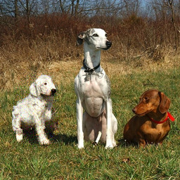
Input image	Image mask	Result 1	Result 2	Result 3	Result 4
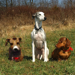
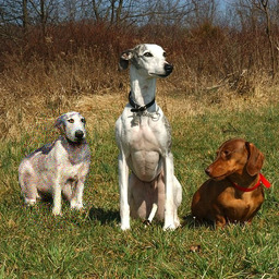
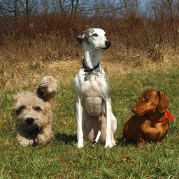
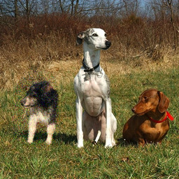
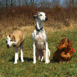
Result 5	Result 6	Result 7	Result 8	Result 9	Result 10

Figure 13: Adding a new object (multiple results for the same input): Given the input image, mask, and text description “a dog”, our model is able to generate multiple plausible results. Some results are better (first row) than others (second row).

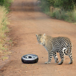
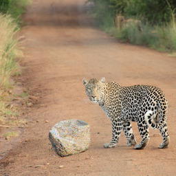
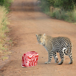
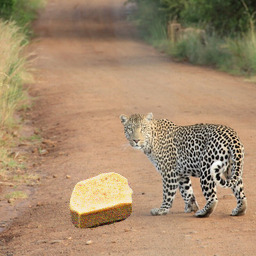
Input image	Input mask	“car tire”	“big stone”	“meat”	“tofu”
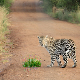
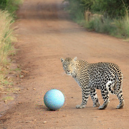
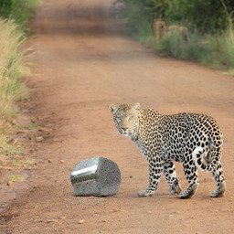
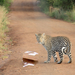
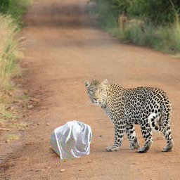
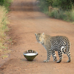
“grass”	“blue ball”	“silver brick”	“ice cube”	“plastic bag”	“bowl of water”
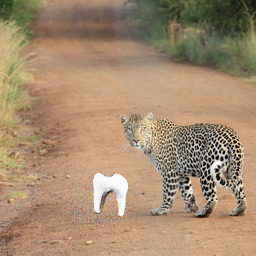
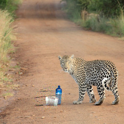
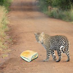
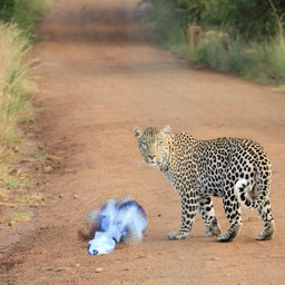
“black rock”	“cardboard”	“tooth”	“water bottle”	“bread”	“smoke”
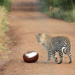
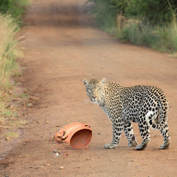
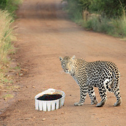
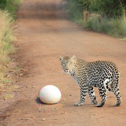
“chocolate”	“clay pot”	“cola”	“egg”	“flower”	“glass”
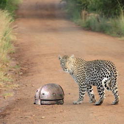
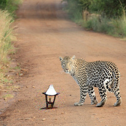
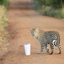
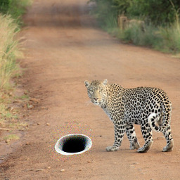
“glow stick”	“gravestone”	“helmet”	“lamp”	“milk”	“hole”

Figure 14: Adding a new object (different prompts): Given an input image and mask, our model is able to generate different objects corresponding to different text descriptions.

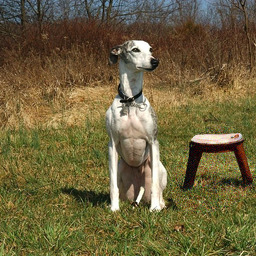
Input image	Input mask	No prompt	“white ball”	“bowl of water”	“stool”
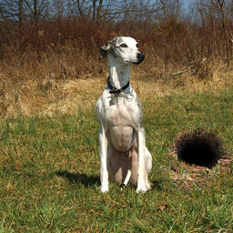
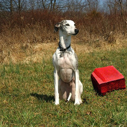
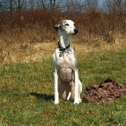
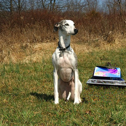
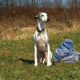
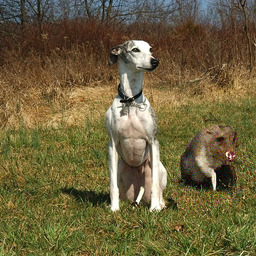
“hole”	“red brick”	“pile of dirt”	“laptop”	“plastic bag”	“rat”
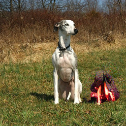
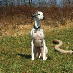
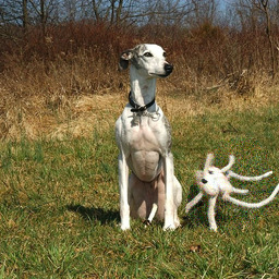
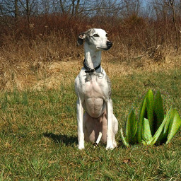
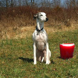
“bonfire”	“snake”	“spider”	“plant”	“candle”	“blanket”
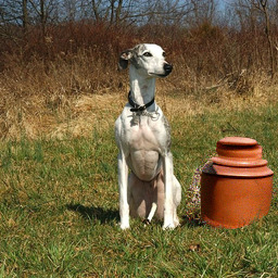
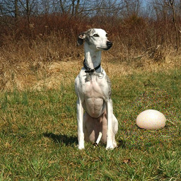
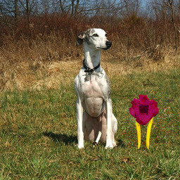
“bottle”	“cardboard”	“chocolate”	“clay pot”	“egg”	“flower”
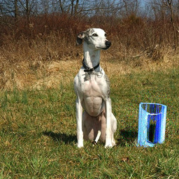
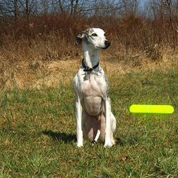
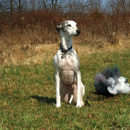
“glass”	“glow stick”	“gravestone”	“helmet”	“milk”	“smoke”

Figure 15: Removing/replacing a foreground object: Given an input image and a mask, we demonstrate inpainting of the masked region using different guiding texts. When no prompt is given, the result is similar to traditional image inpainting.

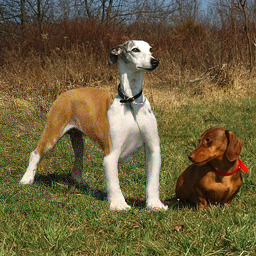
Input image	Input mask	Result 1	Result 2	Result 3	Result 4
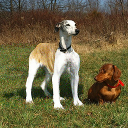
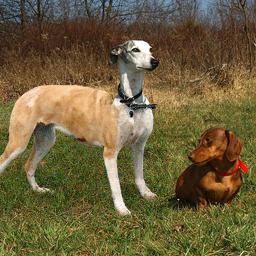
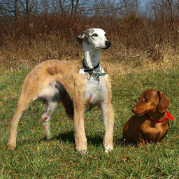
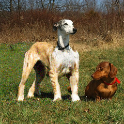
Result 5	Result 6	Result 7	Result 8	Result 9	Result 10
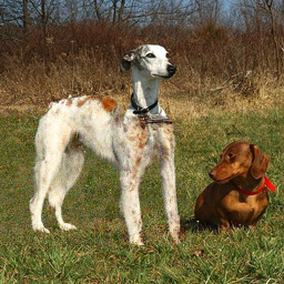
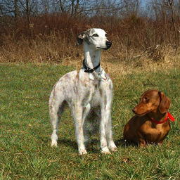
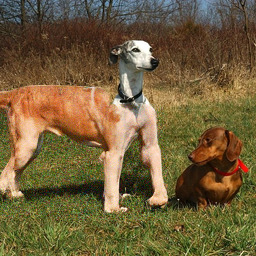
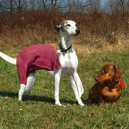
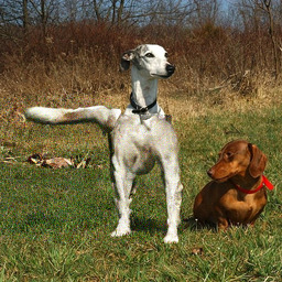
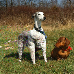
Result 11	Result 12	Result 13	Result 14	Result 15	Result 16
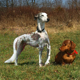
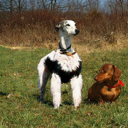
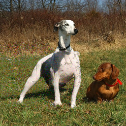
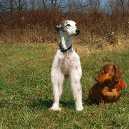
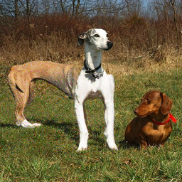
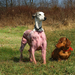
Result 17	Result 18	Result 19	Result 20	Result 21	Result 22

Figure 16: Altering a part of an existing foreground object: Given an input image and a mask, we aim to alter the foreground object corresponding to the guiding text “body of a standing dog”. Multiple plausible results are generated, some more plausible than others. (The first two rows are better than the bottom two rows.)

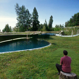
Input image	Input mask	“big mountain”	“swimming pool”	“big wall”	“New York City”
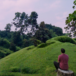
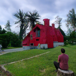
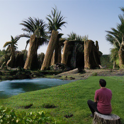
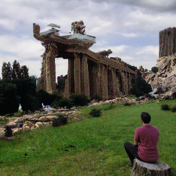
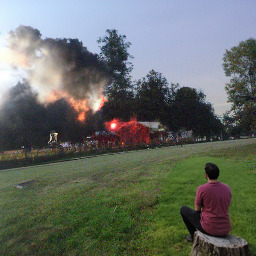
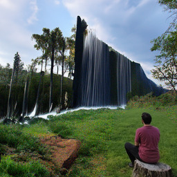
“green hills”	“red house”	“oasis”	“Acropolis”	“fire”	“big waterfall”
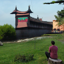
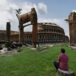
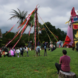
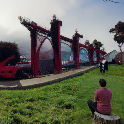
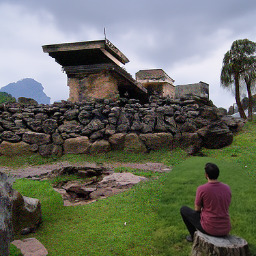
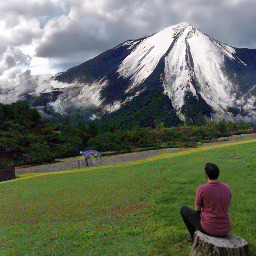
“China”	“Colosseum”	“festival”	“Golden Gate Bridge”	“Machu Picchu”	“Mount Fuji”
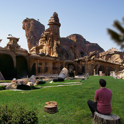
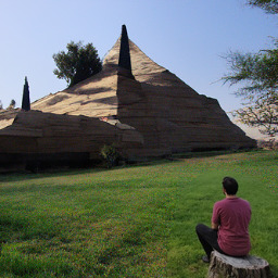
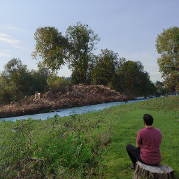
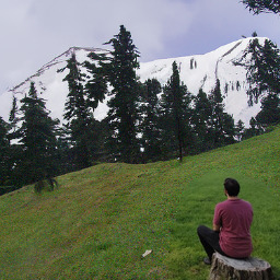
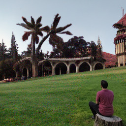
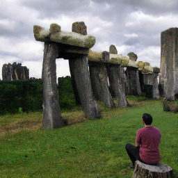
“Petra”	“The Great Pyramid of Giza”	“river”	“snowy mountain”	“Stanford University”	“Stonehenge”
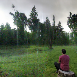
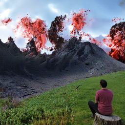
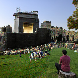
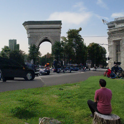
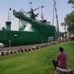
“sunrise”	“rainy”	“volcanic eruption”	“The Western Wall”	“Arc de Triomphe”	“big ship”

Figure 17: Background replacement: Given a source image and a mask of the background, the model is able to replace the background according to the text description. Note that the famous landmarks are not meant to accurately appear in the new background, but serve as an inspiration for the image completion.

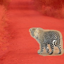
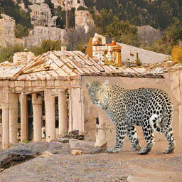
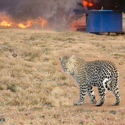
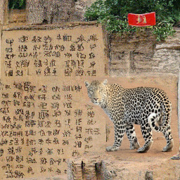
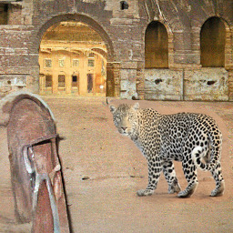
Input image	Input mask	“Acropolis”	“fire”	“China”	“Colosseum”
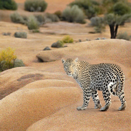
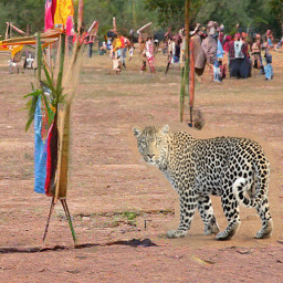
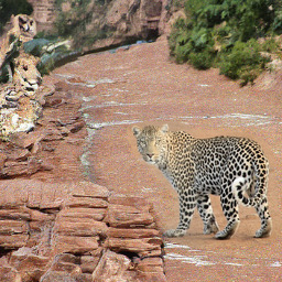
“desert”	“festival”	“Grand Canyon”	“Machu Pichu”	“north pole”	“parking lot”
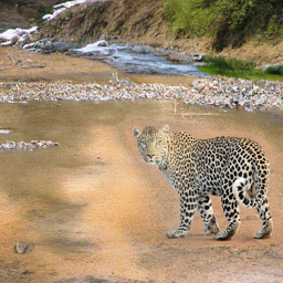
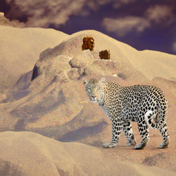
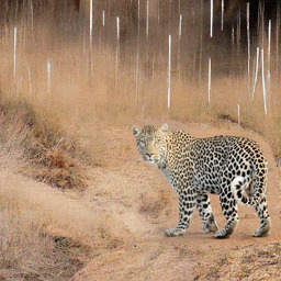
“Petra”	“river”	“snowy mountain”	“Stanford University”	“Stonehenge”	“rainy”
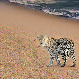
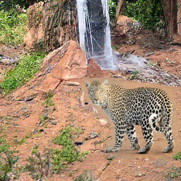
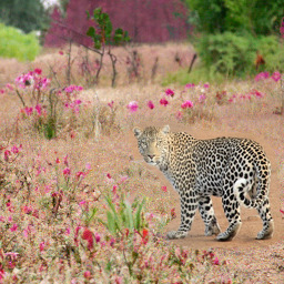
“volcanic eruption”	“The Western Wall”	“in the woods”	“beach”	“big waterfall”	“flower field”
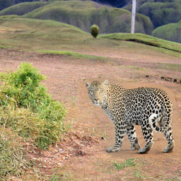
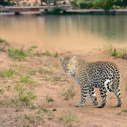
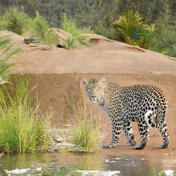
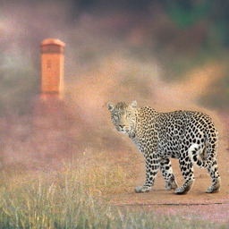
“green hills”	“lake”	“oasis”	“book cover”	“fog”	“gravel”

Figure 18: Background replacement: Given a source image and a mask of the background, the model is able to replace the background corresponding to the text description. Note that the famous landmarks are not meant to accurately appear in the new background, but serve as an inspiration for the image completion.

AAA“leopard”
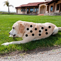
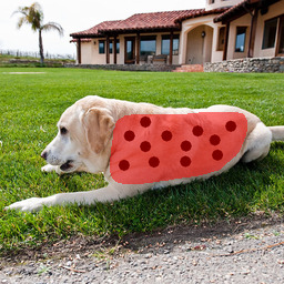
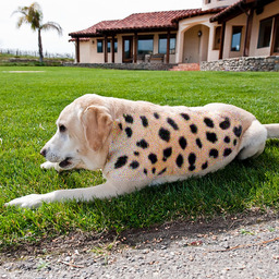
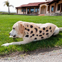
AA“straw chair”
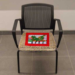
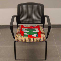
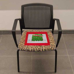
AA“floral carpet”
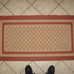
AAA“graffiti”
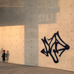
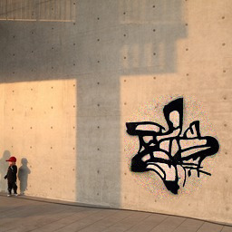
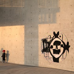
AAA“table”
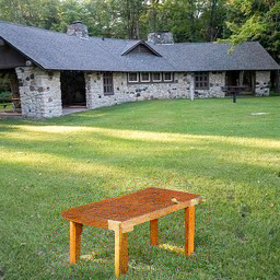
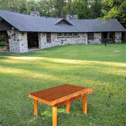
Input image	Image + scribble	Mask	Result 1	Result 2	Result 3

Figure 19: Scribble-guided editing: Users scribble a rough shape of the object they want to insert, mark the edited area, and provide a guiding text. The model uses the scribble as a general shape and color reference, transforming it to match the guiding text. Note that the scribble patterns can also change. In the last example, we embedded a clip art of a table instead of a manual scribble, it shows the effectiveness of our model to transform unnatural clip arts into real-looking objects.

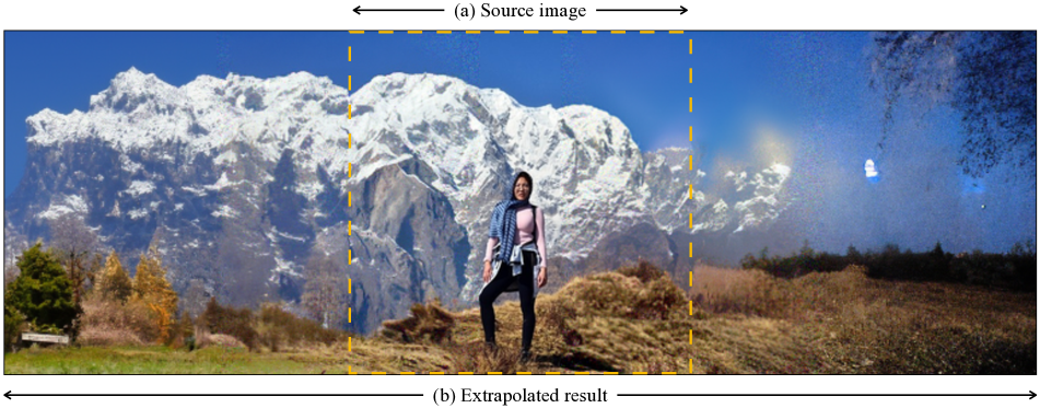
Figure 20: Text-guided image extrapolation: The user provides an image and two text descriptions that guide the extrapolation to the left (“sunny day” in this example) and to the right (“dark night”).

A.2 Iterative Editing

The synthesis results that are given by our method are at times exactly what the user envisioned, but they can also be different from the user’s intent or might include unwanted artifacts. Unlike other text-driven image editing techniques that operate on the entire image (e.g., StyleCLIP [40]), our method is region-based, thus allowing the user to progressively refine their result in an incremental editing session.

Figure 21 demonstrates such an editing session. At first, the user starts by replacing the background, as described in Section 5.3 in the main paper, and obtains a result that is mostly satisfactory, but is not perfect: there are two unwanted generated objects on the grass that the user wishes to remove. In addition, the user decides that the initial mask used in the previous step was not accurate enough, causing a mismatch between the generated grass and the grass from the original scene. The user then provides additional masks, without a text prompt, causing our method to inpaint these areas, yielding the final result.

Figures 22, 23 and 24 demonstrate more editing sessions. Each of the sessions utilizes a variety of editing types: adding, changing and removing objects and backgrounds, scribble-guided edits, and clip-art-guided edits. Out method is compositional by design, and does not require any modifications to support such mixed editing sessions.

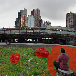
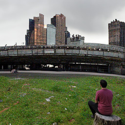
Input image	Input mask	First result	Refinement mask	Final result

Figure 21: Result refinement: The initial synthesis result of our model can be further refined. For example, here the user first masks a rough area in the source image and replaces the background using the prompt “New York City”. Next, they wish to remove two unwanted objects from the generated result and to further refine the rough mask that was used in the first stage. They provide additional masks and no guiding text in this case (to perform inpainting) in order to obtain the final result.

Unless stated otherwise, all the results in the main paper and in this supplemental document are without such incremental refinements — we show the raw results with no further user interaction.

AA Step 1: “curly blond hair”
AA Step 2: “shiny purple tie”
Step 3: scribble + “floral jacket”
Input image	Mask	Result

Figure 22: Editing session mix example: The user can use several editing operations consecutively. For example, as the first step, the user masks the hair of the person and provides the guiding text “curly blond hair”. As the second step, the user masks the tie and provides the guiding text “shiny purple tie”. At the last step, the user scribbles red dots on the jacket, masks the jacket, and provides the guiding text “floral jacket”.

Step 1: paste clip art + “table”
AAAAA Step 2: “orange”
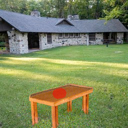
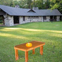
AAA Step 3: “river bank”
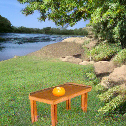
Input image	Mask	Result

Figure 23: Editing session mix example: The user can use several editing operations consecutively. For example, here the user starts by pasting a clip art of a table on the image, then masks the relevant area and provides the guiding text “table” to get a more natural looking table. In the second stage, the user masks an area on the previous synthesis result and provides the guiding text “orange”. In the last stage, the user masks the background of the previous synthesis result and provides the guiding text “river bank” to get the final synthesis result.

AAAAA Step 1: “dresser”
Step 2: scribble + “ceiling lamp”
AAAAA Step 3: “window”
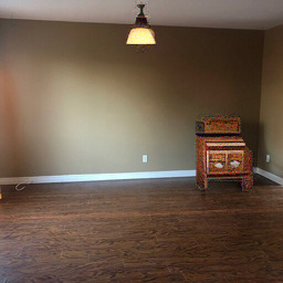
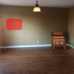
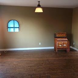
Input image	Mask	Result

Figure 24: Editing session mix example: The user can use several editing operations consecutively. As a first step, the user masks the chair and provides the guiding text “dresser”. Next, the user scribbles a rough shape of a lamp on the result of the previous step, masks the area of the lamp, and provides the guiding text “ceiling lamp”. Finally, the user masks an area over the wall in the previous result, and provides the guiding text “window” to obtain the final result.

A.3 Failure Cases

Figure 25 demonstrates the susceptibility of our model to typographic attacks [19]. Figure 26 demonstrates synthesis of objects which appear natural on their own, but possess the wrong size compared to the rest of the photo.

AAAAA “rubber toy”
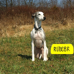
AAAAA “Colosseum”
AAAAA “Acropolis”
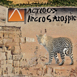
AAAAA “rubber toy”
Input image	Mask	Result

Figure 25: Typographic failure: Our model inherits CLIP [44] susceptibility to typographic attacks [19]. Instead of generating an object or a scene, the model might generate a textual description.

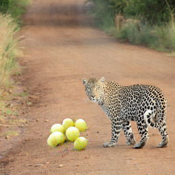
Input image	Mask	Synthesis result

Figure 26: Out of proportion synthesis: We show a failure case in which our method generates objects the look natural by themselves, but with the wrong proportion to the rest of the scene. For the guiding text “grapes”, the synthesized result contains grapes which are huge compared to the leopard and to the rest of the scene.

A.4 Naïve blending example

As discussed in Section 4.2.1 of the paper, naïve blending of the input image and the diffusion-synthesized result inside the masked area yields an unnatural result, as can be seen in Figure 27.

Input image	Input mask	Initial prediction	Naïve blend

Figure 27: Naïve Blending: When providing the model the input image and mask with the text prompt “a dog”, and without using the background preservation loss — the result is a dog whose head is inside the mask, but most of the dog’s body is outside the mask. Blending such a result with the input image using the input mask we obtain an unnatural result.

A.5 High-resolution generation

Most results presented in the paper use an unconditional DDPM model of resolution $256\times 256$, producing generated images of that resolution. Nevertheless, we are not constrained to this resolution, as can be seen in Figure 10 in the main paper and in Figure 20 in this supplementary document (for more details read Section B.5.2). We can also use OpenAI’s unconditional $512\times 512$ version of the model [38], by feeding the one-hot encoding with zeroes vector (similarly to [8]). Demonstration of using the higher resolution model for blended diffusion can be seen in Figure 28.

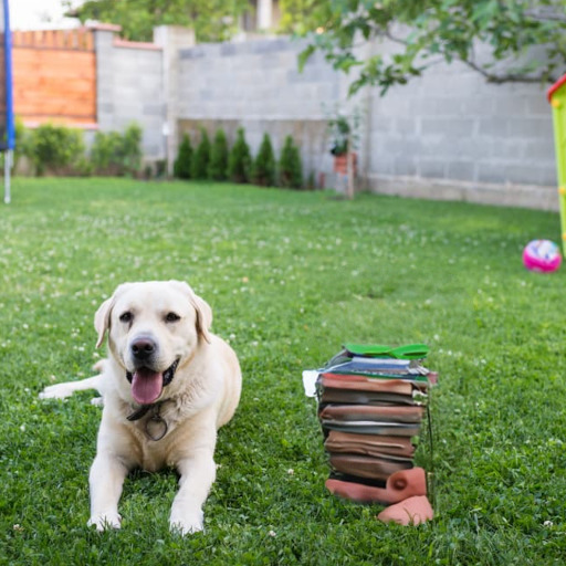
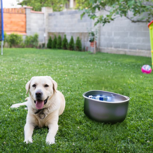
Input image	Input mask	“blanket”	“blue ball”	“pile of books”	“bowl of water”
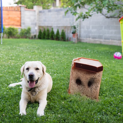
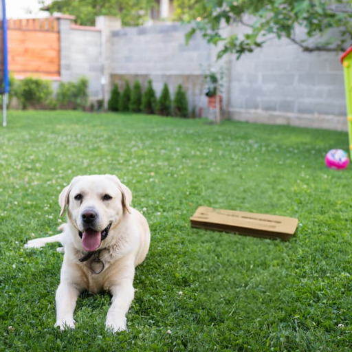
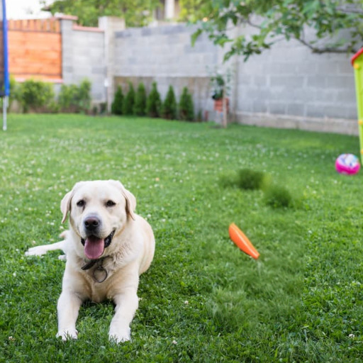
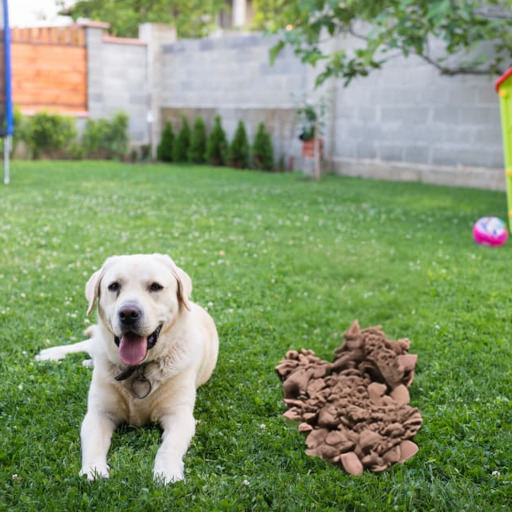
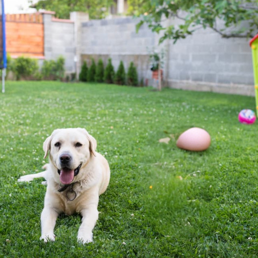
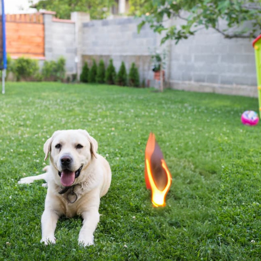
“bread”	“cardboard”	“carrot”	“pile of dirt”	“egg”	“fire”
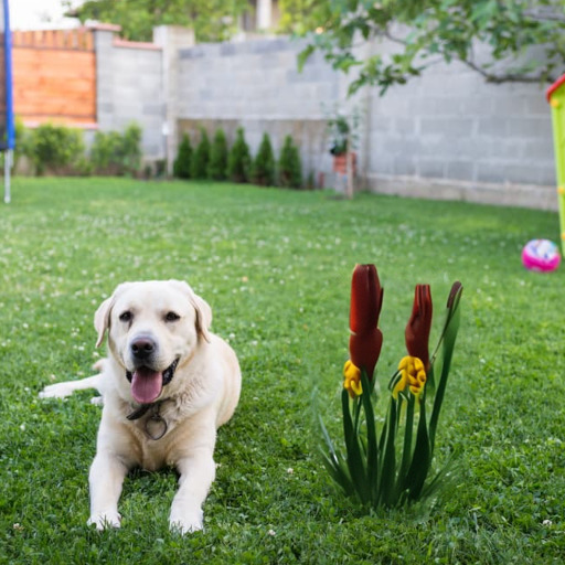
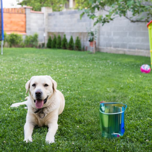
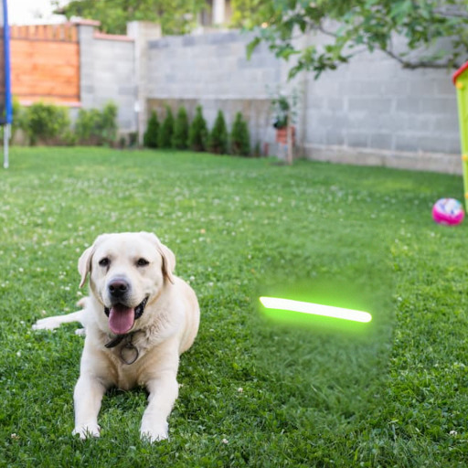
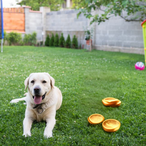
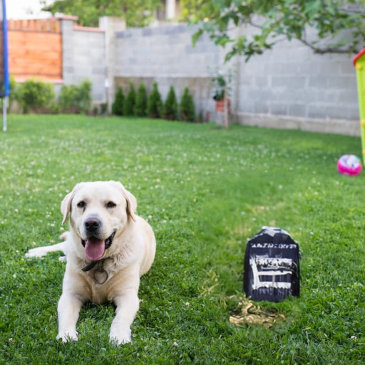
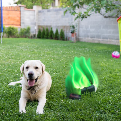
“flower”	“glass”	“glow stick”	“golden coins”	“grave”	“green flame”
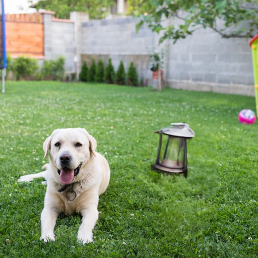
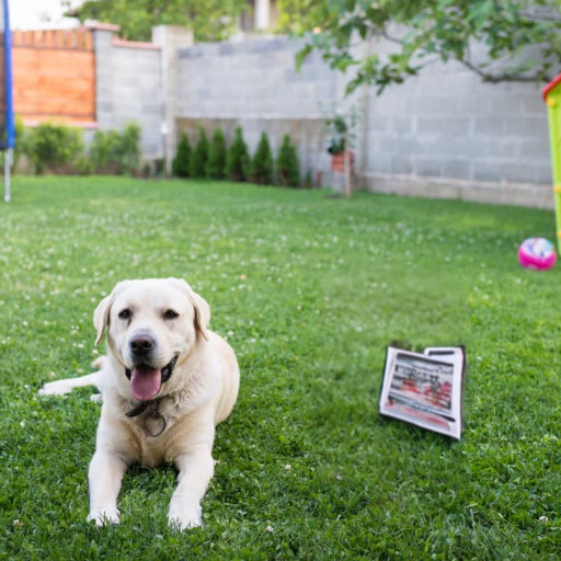
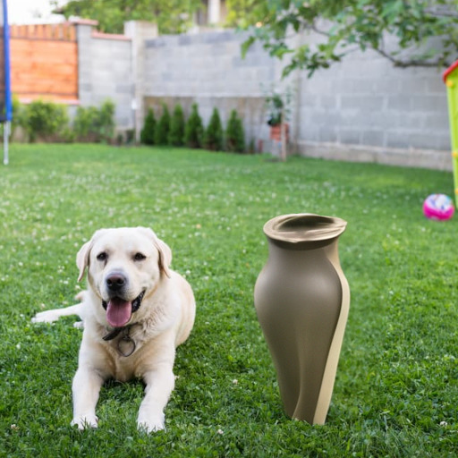
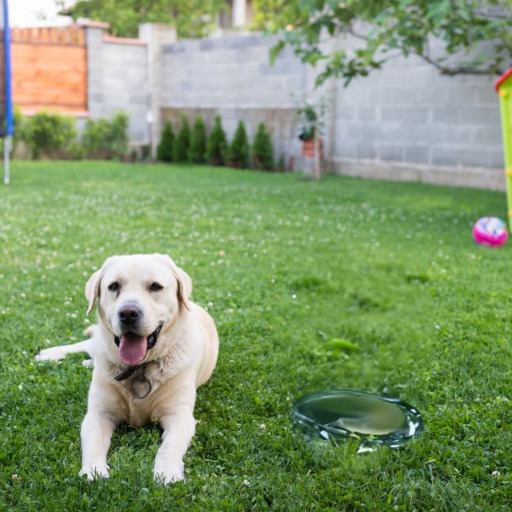
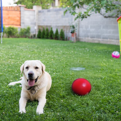
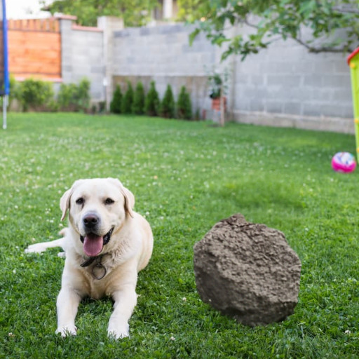
“lamp”	“newspaper”	“clay pot”	“puddle”	“red ball”	“rock”
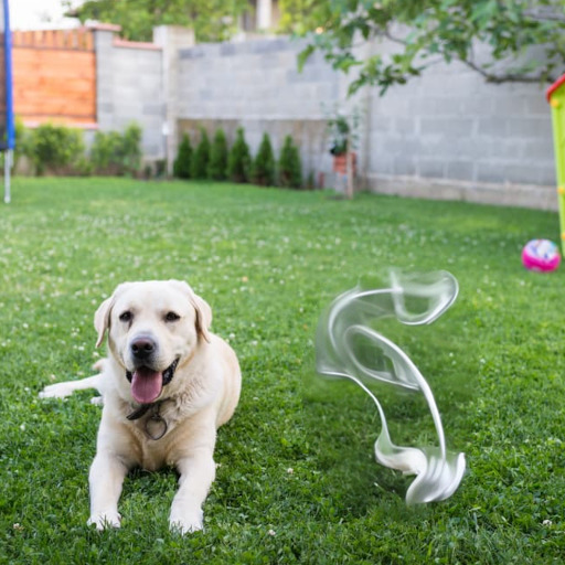
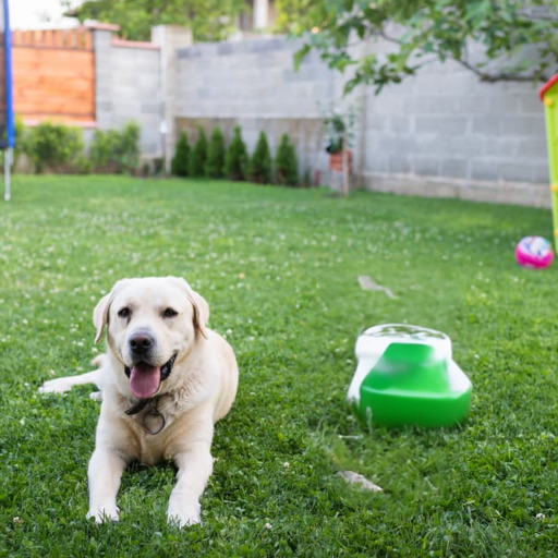
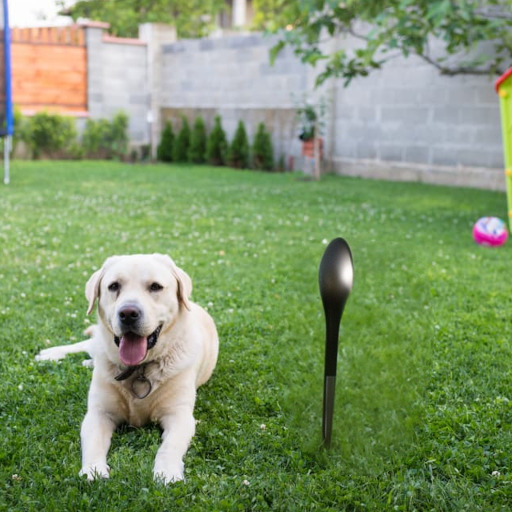
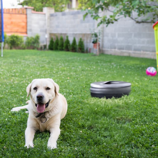
“smoke”	“soap”	“spoon”	“car tire”	“vase”	“shiny ball”

Figure 28: High resolution results: Given an input image of and mask, our model is able to generate different objects corresponding to different text descriptions. Results were produced using $512\times 512$ DDPM model.

A.6 Comparison to DDIM

Our method uses Denoising Diffusion Probabilistic Models (DDPMs). Recently, Song et al. propose Denoising Diffusion Implicit Models (DDIMs) [50], a fast sampling algorithm for DDPMs that produces a new implicit model with the same marginal noise distributions, but deterministically maps noise to images. Nichol et al. [36] showed that DDIMs produce better samples than DDPMs with fewer than 50 sampling steps, but worse samples when using 50 or more steps. In order to check the effect of using DDIM instead of DDPM we first adjusted the DDIM version of the guided-diffusion algorithm [11] with Blended Diffusion in Algorithm 3. As we can see experimentally in Figure 29, the same holds for image generation using Blended Diffusion: DDPMs produce better results than DDIMs when using 100 diffusion steps, but worse results when using less than 50 diffusion steps.

Algorithm 3 DDIM blended diffusion: given a diffusion model $(\mu_{\theta}(x_{t}),\Sigma_{\theta}(x_{t}))$, and $\mathit{CLIP}$ model

  Input: source image $x$, target text description $d$, input mask $m$, diffusion steps $k$, number of extending augmentations $N$

  Output: edited image $\widehat{x}$ that differs from input image $x$ inside area $m$ according to text description $d$

  $x_{k}\sim\mathcal{N}(\sqrt{\bar{\alpha}_{k}}x_{0},(1-\bar{\alpha}_{k})\mathbf{I})$

  for all $t$ from $k$ to 0 do

     $\mu,\Sigma\leftarrow\mu_{\theta}(x_{t}),\Sigma_{\theta}(x_{t})$

     $\widehat{x}_{0}\leftarrow\frac{x_{t}}{\sqrt{\bar{\alpha}_{t}}}-\frac{\sqrt{1-\bar{\alpha}_{t}}\epsilon_{\theta}(x_{t},t)}{\sqrt{\bar{\alpha}_{t}}}$

     $\widehat{x}_{0,{\textit{aug}}}\leftarrow{\textit{ExtendingAugmentations}(\widehat{x}_{0},N)}$

     $\nabla_{\textit{text}}\leftarrow\frac{1}{N}\sum_{i=1}^{N}\nabla_{\widehat{x}_{0,{\textit{aug}}}}\mathcal{D}_{\textit{CLIP}}(\widehat{x}_{0,{\textit{aug}}},d,m)$

     $\hat{\epsilon}\leftarrow\epsilon_{\theta}(x_{t})-\sqrt{1-\bar{\alpha}_{t}}\nabla_{\textit{text}}$

     $x_{\textit{fg}}\leftarrow\sqrt{\bar{\alpha}_{t-1}}\left(\frac{x_{t}-\sqrt{1-\bar{\alpha}_{t}}\hat{\epsilon}}{\sqrt{\bar{\alpha}_{t}}}\right)+\sqrt{1-\bar{\alpha}_{t-1}}\hat{\epsilon}$

     $x_{\textit{bg}}\sim\mathcal{N}(\sqrt{\bar{\alpha}_{t}}x_{0},(1-\bar{\alpha}_{t})\mathbf{I})$

     $x_{t-1}\leftarrow x_{\textit{fg}}\odot m+x_{\textit{bg}}\odot(1-m)$

  end for

  return  $x_{-1}$

AAADDPM
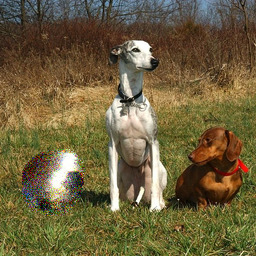
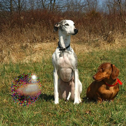
AAADDIM
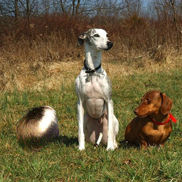
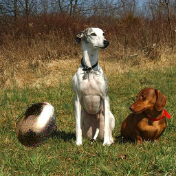
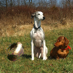
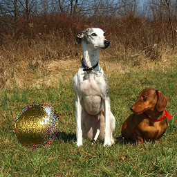
AAADDPM
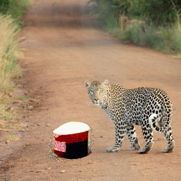
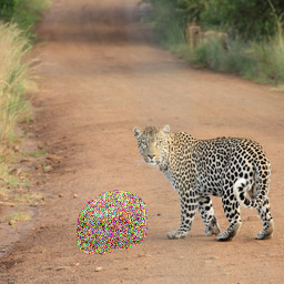
AAADDIM
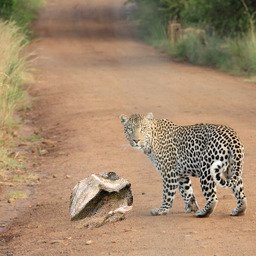
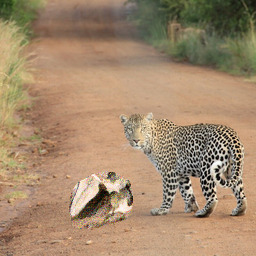
AAADDPM
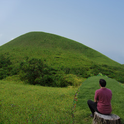
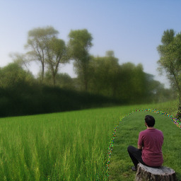
AAADDIM
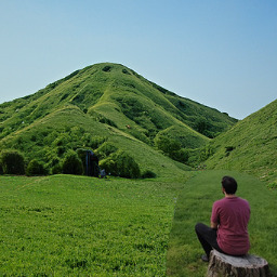
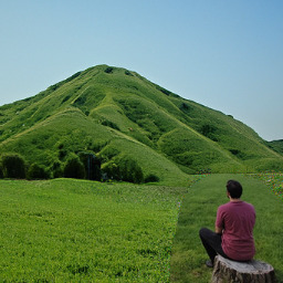
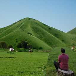
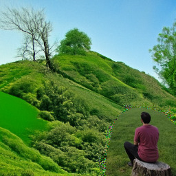
	Input image	Input mask	100 steps	50 steps	25 steps	12 steps

Figure 29: Blended Diffusion DDPM VS Blended Diffusion DDIM comparison: The part corresponds to the editing text “a shiny ball”, the middle part to “a rock” and the bottom part to “green hills”. As we can see, DDPM produces better results when using 100 diffusion steps, whereas it produces worse results in less than 50 diffusion steps.

Appendix B Implementation Details

For all the experiments reported in this paper we used a pre-trained CLIP model [44] and a pre-trained guided-diffusion model [11]:

• For the CLIP model we used ViT-B/16 as a backbone for the Vision Transformer [13] that was released by OpenAI [37].

• For the diffusion model we used an unconditional model of resolution $256\times 256$ [38].

Both of these models were released under MIT license and were developed using PyTorch [39].

All the input images in this paper are real images (i.e., not synthesized), except the ones in Figure 5 of the main paper, which were generated by Bau et al. [4]. All images were released freely under a Creative Commons license.

B.1 Hyperparamters

We used the CLIP model as-is, without changing any parameters. In addition, we did not utilize any prompt engineering techniques as described by Radford et al. [44].

We used the following hyperparameters in the guided-diffusion model across the different experiments (both in our model and in the baselines):

• Fast sampling speed: We follow the fast sampling speed from [36] which showed that 100 sampling steps are sufficient to achieve near-optimal FID score [23] on ImageNet [10]. This scheme reduces the sampling time to 27 seconds, for more details see Section B.3.

• Number of diffusion steps: In most of our experiments we set the number of diffusion steps to $k=75$, allowing the model to change the input image in a sufficient manner. Exceptions are scribble-based editing ($k=60$) and background editing ($k=67$).

In Algorithm 2 we use the following hyperparameters:

• Number of extending augmentations: We found that setting this to $N=16$ was sufficient to mitigate the adversarial example phenomena.

• Number of total repetitions: As explained in Section 4.2.3, we generate several results and rank them using the CLIP model. In our experiments, we generate 64 samples and choose the best ones. For more details on inference time see Section B.3.

B.2 Extending Augmentations

Given an input image $x$, in the resolution of the diffusion model ($256\times 256$ in our case), we first resize it to the input size of the CLIP model ($224\times 224$) along with its input mask. Next, we create $N$ copies of this image and perform a different random projective transformation on each copy, along with the same transformation on the corresponding mask (see Figure 30). Finally, we calculate the gradients using the CLIP loss w.r.t each one of the transformed copies and average all the gradients. This way, an adversarial manipulation is much less likely, as it would have to “fool” CLIP under multiple transformations.

Input + mask	Augmentation 1	Augmentation 2	Augmentation 3

Figure 30: Extending augmentation example: Given an input image and mask, we augment the masked area in the image using various projective transformations.

As mentioned in Section 5.2 we performed an ablation study for the extending augmentations. Figure 31 demonstrates the importance of the augmentations: the same random seed is used in two runs, one with and the other without augmentations. We can see that the images generated with the use of augmentations are more visually plausible and are more coherent than the ones generated without the augmentations. (This is an extended version of Figure 7 from the main paper.)

AAA “big red pillow”
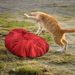
Aa “happy dog mouth”
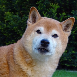
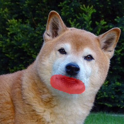
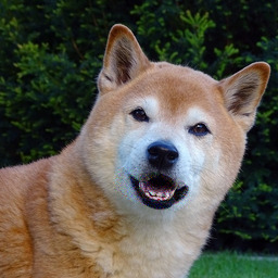
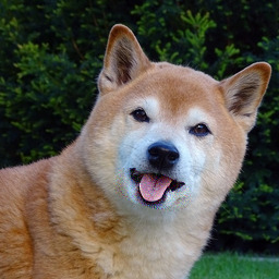
AAAA “sausages”
AAA “huge avocado”
AAA “knit beanie”
AAA“burning tree”
Input image	Input image + mask	(1)	(2)

Figure 31: Extending augmentations ablation: In order to assess the importance of the extending augmentation technique, we used the same random seeds for the same inputs to ensure that the results would differ in the use of augmentations. As we can see, (2) using extending augmentations makes the resulting images more natural and coherent with the background in comparison to (1) not using extending augmentations.

B.3 Inference Time

We report synthesis time for a single image using one NVIDIA A10 GPU:

• Our method (Algorithm 2) & Local CLIP-guided diffusion (Algorithm 1): 27 seconds.

• PaintByWord++: 78 seconds.

Original paint by word [4] did not release their code and did not mention the run-time.

In practice, as described in Section 4.2.3, we generate several results for the same inputs and use the best ones. Instead of generating them sequentially, we accelerate the generation process using two techniques:

1. Batch generation: Instead of generating a single image in each diffusion pass, we multiplied the input several times and generated several instances on the same pass. Because of the stochasticity of the diffusion process, each result is different.

2. Parallel generation: Because each of the generation processes is independent, we can distribute the generation across multiple GPUs. In our experiments, we concurrently used 4 NVIDIA A10 GPUs.

Using the above accelerations, we generate 64 synthesis results in about 6 minutes — less than 6 seconds per image.

B.4 Comparison with Baselines

PaintByWord

Because the models and code that was used by Bau et al. [4] are currently unavailable, we used as input the images and masks extracted from their paper.

PaintByWord++

We adapted the VQGAN+CLIP [9] implementation to support masks using the same $\mathcal{D}_{\textit{CLIP}}$ loss from Equation 6. We used the VQGAN [14] model that was trained on ImageNet with reduction factor $f=16$. For the latent optimization, we used the Adam optimizer with a learning rate of 0.1 for 500 steps. We found that constraining the optimization of the latent space $z$ only to the corresponding mask area, the same way it was done by Bau et al. [4], improved the background preservation.

B.5 Implementation Details for Applications

In this section, we provide the implementation details for scribble-guided editing and text-guided image extrapolation applications.

B.5.1 Scribble-guided editing

In order to create the results that are demonstrated in Figure 9 of the main paper, the user first scribbles on the input image, then masks the scribble area (the masking can also be done automatically by taking the scribbles area and dilating it by morphological operations), then provides a text prompt and uses the same algorithm as for object altering.

An important hyper-parameter for this application is the number of target diffusion steps $k$ in Algorithm 2. Figure 32 demonstrates the effect of changing this parameter: when diffusing for a longer period (e.g., 80 diffusion steps out of 100), only the main red color of the blanket is kept, the blanket shading is more realistic, and the results are more diverse. When diffusing for a shorter period (e.g., 20 diffusion steps out of 100), the scribble is hardly modified.

Original image	Input scribble	Mask

ADiffusion steps $k=20$
ADiffusion steps $k=40$
ADiffusion steps $k=60$
ADiffusion steps $k=80$
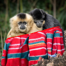
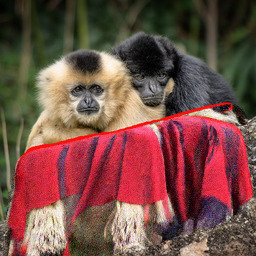
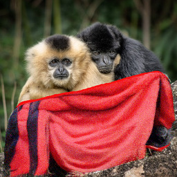
Result 1	Result 2	Result 3	Result 4

Figure 32: Scribble-guided editing diffusion steps effect: when the diffusion steps are large (e.g. $k=80$), the resulting images are more realistic and diverse but do not preserve the colors of the input scribble, on the other hand, when the diffusions steps are low (e.g. $k=20$), the resulting images are almost identical to the input scribble.

B.5.2 Text-guided image extrapolation

In order to extend the image beyond its original resolution, we gradually predict the unknown parts of the image in a sequential manner. Figure 33 demonstrates the building process: at each stage, (2) we translate the image $\frac{1}{4}$ to the opposite of the desired direction and fill the missing area using standard reflection padding, (4) then we inpaint the new area guided by the text description, using the regular algorithm for foreground editing. (5-7) We repeat the process 3 times until we have a new image. The new image is still a bit noisy — due of the gradual inpainting, each synthesis result is noisier than the previous one because of the chaining of the natural image statistics. In order to mitigate it, (8) we denoise this image using the diffusion process again. We repeat the same process in the other direction. Our output can have an arbitrarily large image resolution.

We also notice that gradual diffusion steps are beneficial: we diffuse the first quarter for a small number of diffusion steps, and then in each step, we enlarge the number of diffusion steps.

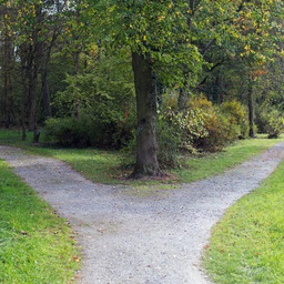
(1) Source image	(2) Translated and reflected	(3) Mask	(4) 1st prediction
(5) 2nd prediction	(6) 3rd prediction	(7) 4th prediction	(8) Denoised prediction

Figure 33: Text-guided image extrapolation: We aim to extrapolate the source image (1) to the right according to the guiding text “heaven”. We start by (2) translating the image to the left by $\frac{1}{4}$ of the input resolution, and filling the missing area with reflection padding. Then we mask the new area (3) and predict the missing part (4) using the foreground altering algorithm. We perform this process 3 more times (5-7) to get a noisy prediction (7). In order to denoise it, we do the same process with a mask that covers the entire image and get the denoised result (8) that we can stitch to the source image. Notice that we can reach an arbitrary resolution using this method.

B.6 Ranking Implementation Details

We utilized the ranking algorithm that is explained in Section 4.2.3 in the main paper using 64 synthesis results. As described in Section 6 in the main paper, the ranking is not perfect because it takes into account only the generated area. In addition, the ranking is not accurate enough in the resolution of single images: the top-ranked image isn’t always better than the second one, etc. Nonetheless, the top 20% of the images are almost always better than the bottom 20%. In practice, we generate 64 results and choose manually from the top 10 images ordered by their ranking (in both the baselines and our method). Figure 34 demonstrates the effectiveness of the ranking algorithm.

Aa“pile of books”
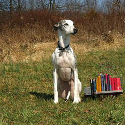
AA“car tire”
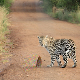
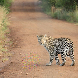
AAA“sunrise”
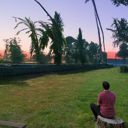
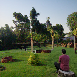
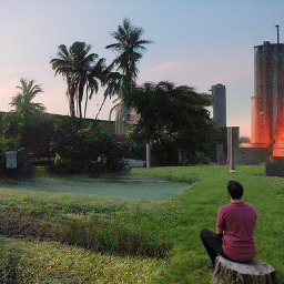
AAA“gravel”
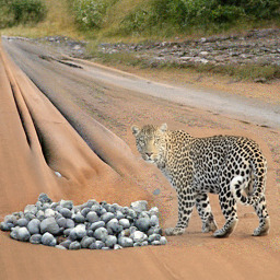
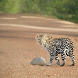
Input image	Input mask	1st ranked result	2nd ranked result	63th ranked result	64th ranked result

Figure 34: Ranking algorithm effectiveness: We generate 64 synthesis results and rank them using CLIP. We found that this method only roughly ranks the results: the top 20% are consistently better than the bottom 20%, but in the resolution of a single image, this is not the case — the first result isn’t always better than the second one.

Appendix C User Study

In order to evaluate our model quantitatively, we conducted a user study. The only results of the Paint By Word model on general images (albeit GAN-generated) that were available are the ones in their paper. Hence, we chose to conduct the user study on these images (along with their corresponding masks). The study was conducted on 35 participants.

The participants were shown each time the inputs to the model (image, mask and text description) along with the model prediction, and were asked to rate the prediction, on a scale of 1–5, for one of the following criteria:

1. The overall realism of the prediction.

2. The amount of background preservation of the prediction in the unedited area.

3. The correspondence of the edited image to the guiding text description.

The questions were randomly ordered, and the participant had the ability to go back and edit their previous ratings until submission.

Mean user study scores are presented in Table 1 of the main paper. The difference between conditions is statistically significant (Kruskal-Wallis test, $p<10^{-130}$). Further analysis using Tukey’s honestly significant difference procedure [54] shows that the improvement shown by our method is statistically significant vs. all other conditions (Table 2).

Method 1	Method 2	Realism	Background preservation	Text match
		p-value	p-value	p-value
Local CLIP GD [8]	Ours	0.003	¡0.001	¡0.001
Local CLIP GD [8]	PaintByWord [4]	0.435	0.578	¡0.001
Local CLIP GD [8]	PaintByWord++ [9, 4]	¡0.001	0.106	¡0.001
Ours	PaintByWord [4]	¡0.001	¡0.001	¡0.001
Ours	PaintByWord++ [9, 4]	¡0.001	¡0.001	¡0.001
PaintByWord [4]	PaintByWord++ [9, 4]	¡0.001	0.719	0.704

Table 2: User study statistical analysis: We use Tukey’s honestly significant difference procedure [54] to test whether the differences between mean scores in our user study are statistically significant. Significant results in bold. Our results are statistically better than all other methods on all the measured conditions.

References

- [1] Rameen Abdal, Yipeng Qin, and Peter Wonka. Image2stylegan: How to embed images into the StyleGAN latent space? In Proceedings of the IEEE/CVF International Conference on Computer Vision, pages 4432–4441, 2019.
- [2] Rameen Abdal, Yipeng Qin, and Peter Wonka. Image2stylegan++: How to edit the embedded images? In Proceedings of the IEEE/CVF Conference on Computer Vision and Pattern Recognition, pages 8296–8305, 2020.
- [3] Yuval Alaluf, Or Patashnik, and Daniel Cohen-Or. Restyle: A residual-based StyleGAN encoder via iterative refinement. In Proceedings of the IEEE/CVF International Conference on Computer Vision, pages 6711–6720, 2021.
- [4] David Bau, Alex Andonian, Audrey Cui, YeonHwan Park, Ali Jahanian, Aude Oliva, and Antonio Torralba. Paint by word. arXiv preprint arXiv:2103.10951, 2021.
- [5] Aaron Blake. Trump is reportedly suggesting the ‘access hollywood’ tape was fake news. https://www.washingtonpost.com/news/the-fix/wp/2017/11/27/trump-is-reportedly-saying-the-access-hollywood-tape-was-fake-news-he-should-talk-to-2016-trump/. Accessed: 2021-11-15.
- [6] Andrew Brock, Jeff Donahue, and Karen Simonyan. Large scale GAN training for high fidelity natural image synthesis. arXiv preprint arXiv:1809.11096, 2018.
- [7] Peter J Burt and Edward H Adelson. The Laplacian pyramid as a compact image code. In Readings in computer vision, pages 671–679. Elsevier, 1987.
- [8] Katherine Crowson. CLIP guided diffusion HQ 256x256. https://colab.research.google.com/drive/12a_Wrfi2_gwwAuN3VvMTwVMz9TfqctNj.
- [9] Katherine Crowson. VQGAN+CLIP. https://colab.research.google.com/drive/1L8oL-vLJXVcRzCFbPwOoMkPKJ8-aYdPN.
- [10] Jia Deng, Wei Dong, Richard Socher, Li-Jia Li, Kai Li, and Li Fei-Fei. Imagenet: A large-scale hierarchical image database. In 2009 IEEE conference on computer vision and pattern recognition, pages 248–255. Ieee, 2009.
- [11] Prafulla Dhariwal and Alexander Nichol. Diffusion models beat gans on image synthesis. Advances in Neural Information Processing Systems, 34, 2021.
- [12] Ming Ding, Zhuoyi Yang, Wenyi Hong, Wendi Zheng, Chang Zhou, Da Yin, Junyang Lin, Xu Zou, Zhou Shao, Hongxia Yang, et al. Cogview: Mastering text-to-image generation via transformers. arXiv preprint arXiv:2105.13290, 2021.
- [13] Alexey Dosovitskiy, Lucas Beyer, Alexander Kolesnikov, Dirk Weissenborn, Xiaohua Zhai, Thomas Unterthiner, Mostafa Dehghani, Matthias Minderer, Georg Heigold, Sylvain Gelly, et al. An image is worth 16x16 words: Transformers for image recognition at scale. In International Conference on Learning Representations, 2020.
- [14] Patrick Esser, Robin Rombach, and Bjorn Ommer. Taming transformers for high-resolution image synthesis. In Proceedings of the IEEE/CVF Conference on Computer Vision and Pattern Recognition, pages 12873–12883, 2021.
- [15] Zeev Farbman, Gil Hoffer, Yaron Lipman, Daniel Cohen-Or, and Dani Lischinski. Coordinates for instant image cloning. ACM Trans. Graph., 28(3), July 2009.
- [16] Hany Farid. Digital doctoring: can we trust photographs? 2009.
- [17] W Feller. On the theory of stochastic processes, with particular reference to applications. In First Berkeley Symposium on Mathematical Statistics and Probability, pages 403–432, 1949.
- [18] Ohad Fried, Jennifer Jacobs, Adam Finkelstein, and Maneesh Agrawala. Editing self-image. volume 63, page 70–79, New York, NY, USA, Feb. 2020. Association for Computing Machinery.
- [19] Gabriel Goh, Nick Cammarata, Chelsea Voss, Shan Carter, Michael Petrov, Ludwig Schubert, Alec Radford, and Chris Olah. Multimodal neurons in artificial neural networks. Distill, 2021. https://distill.pub/2021/multimodal-neurons.
- [20] Ian Goodfellow, Jean Pouget-Abadie, Mehdi Mirza, Bing Xu, David Warde-Farley, Sherjil Ozair, Aaron Courville, and Yoshua Bengio. Generative adversarial nets. Advances in neural information processing systems, 27, 2014.
- [21] Ian J Goodfellow, Jonathon Shlens, and Christian Szegedy. Explaining and harnessing adversarial examples. arXiv preprint arXiv:1412.6572, 2014.
- [22] James Hays and Alexei A. Efros. Scene completion using millions of photographs. ACM Trans. Graph., 26(3):4–es, July 2007.
- [23] Martin Heusel, Hubert Ramsauer, Thomas Unterthiner, Bernhard Nessler, and Sepp Hochreiter. GANs trained by a two time-scale update rule converge to a local nash equilibrium. Advances in neural information processing systems, 30, 2017.
- [24] Tobias Hinz, Stefan Heinrich, and Stefan Wermter. Semantic object accuracy for generative text-to-image synthesis. arXiv preprint arXiv:1910.13321, 2019.
- [25] Jonathan Ho, Ajay Jain, and Pieter Abbeel. Denoising diffusion probabilistic models. In NeurIPS, 2020.
- [26] Tero Karras, Miika Aittala, Samuli Laine, Erik Härkönen, Janne Hellsten, Jaakko Lehtinen, and Timo Aila. Alias-free generative adversarial networks. arXiv preprint arXiv:2106.12423, 2021.
- [27] Tero Karras, Samuli Laine, and Timo Aila. A style-based generator architecture for generative adversarial networks. In Proceedings of the IEEE/CVF Conference on Computer Vision and Pattern Recognition, pages 4401–4410, 2019.
- [28] Tero Karras, Samuli Laine, Miika Aittala, Janne Hellsten, Jaakko Lehtinen, and Timo Aila. Analyzing and improving the image quality of StyleGAN. In Proceedings of the IEEE/CVF Conference on Computer Vision and Pattern Recognition, pages 8110–8119, 2020.
- [29] Gwanghyun Kim and Jong Chul Ye. Diffusionclip: Text-guided image manipulation using diffusion models. arXiv preprint arXiv:2110.02711, 2021.
- [30] Bowen Li, Xiaojuan Qi, Thomas Lukasiewicz, and Philip HS Torr. Controllable text-to-image generation. arXiv preprint arXiv:1909.07083, 2019.
- [31] Wenbo Li, Pengchuan Zhang, Lei Zhang, Qiuyuan Huang, Xiaodong He, Siwei Lyu, and Jianfeng Gao. Object-driven text-to-image synthesis via adversarial training. In Proceedings of the IEEE/CVF Conference on Computer Vision and Pattern Recognition, pages 12174–12182, 2019.
- [32] Xihui Liu, Dong Huk Park, Samaneh Azadi, Gong Zhang, Arman Chopikyan, Yuxiao Hu, Humphrey Shi, Anna Rohrbach, and Trevor Darrell. More control for free! image synthesis with semantic diffusion guidance. arXiv preprint arXiv:2112.05744, 2021.
- [33] Elman Mansimov, Emilio Parisotto, Jimmy Ba, and Ruslan Salakhutdinov. Generating images from captions with attention. CoRR, abs/1511.02793, 2016.
- [34] Ryan Murdock. The big sleep: BigGANxCLIP. https://colab.research.google.com/github/levindabhi/CLIP-Notebooks/blob/main/The_Big_Sleep_BigGANxCLIP.ipynb.
- [35] Alex Nichol, Prafulla Dhariwal, Aditya Ramesh, Pranav Shyam, Pamela Mishkin, Bob McGrew, Ilya Sutskever, and Mark Chen. Glide: Towards photorealistic image generation and editing with text-guided diffusion models. arXiv preprint arXiv:2112.10741, 2021.
- [36] Alexander Quinn Nichol and Prafulla Dhariwal. Improved denoising diffusion probabilistic models. In International Conference on Machine Learning, pages 8162–8171. PMLR, 2021.
- [37] OpenAI. CLIP Github. https://github.com/openai/CLIP.
- [38] OpenAI. Guided Diffusion Github. https://github.com/openai/guided-diffusion.
- [39] Adam Paszke, Sam Gross, Francisco Massa, Adam Lerer, James Bradbury, Gregory Chanan, Trevor Killeen, Zeming Lin, Natalia Gimelshein, Luca Antiga, et al. Pytorch: An imperative style, high-performance deep learning library. Advances in neural information processing systems, 32:8026–8037, 2019.
- [40] Or Patashnik, Zongze Wu, Eli Shechtman, Daniel Cohen-Or, and Dani Lischinski. StyleCLIP: Text-driven manipulation of StyleGAN imagery. In Proceedings of the IEEE/CVF International Conference on Computer Vision, pages 2085–2094, 2021.
- [41] Patrick Pérez, Michel Gangnet, and Andrew Blake. Poisson image editing. ACM Trans. Graph., 22(3):313–318, July 2003.
- [42] Tingting Qiao, Jing Zhang, Duanqing Xu, and Dacheng Tao. Learn, imagine and create: Text-to-image generation from prior knowledge. Advances in Neural Information Processing Systems, 32:887–897, 2019.
- [43] Tingting Qiao, Jing Zhang, Duanqing Xu, and Dacheng Tao. MirrorGAN: Learning text-to-image generation by redescription. In Proceedings of the IEEE/CVF Conference on Computer Vision and Pattern Recognition, pages 1505–1514, 2019.
- [44] Alec Radford, Jong Wook Kim, Chris Hallacy, Aditya Ramesh, Gabriel Goh, Sandhini Agarwal, Girish Sastry, Amanda Askell, Pamela Mishkin, Jack Clark, et al. Learning transferable visual models from natural language supervision. arXiv preprint arXiv:2103.00020, 2021.
- [45] Aditya Ramesh, Mikhail Pavlov, Gabriel Goh, Scott Gray, Chelsea Voss, Alec Radford, Mark Chen, and Ilya Sutskever. Zero-shot text-to-image generation. arXiv preprint arXiv:2102.12092, 2021.
- [46] Ali Razavi, Aaron van den Oord, and Oriol Vinyals. Generating diverse high-fidelity images with VQ-VAE-2. In Advances in neural information processing systems, pages 14866–14876, 2019.
- [47] Scott Reed, Zeynep Akata, Xinchen Yan, Lajanugen Logeswaran, Bernt Schiele, and Honglak Lee. Generative adversarial text to image synthesis. In International Conference on Machine Learning, pages 1060–1069. PMLR, 2016.
- [48] Elad Richardson, Yuval Alaluf, Or Patashnik, Yotam Nitzan, Yaniv Azar, Stav Shapiro, and Daniel Cohen-Or. Encoding in style: a StyleGAN encoder for image-to-image translation. In Proceedings of the IEEE/CVF Conference on Computer Vision and Pattern Recognition, pages 2287–2296, 2021.
- [49] Jascha Sohl-Dickstein, Eric Weiss, Niru Maheswaranathan, and Surya Ganguli. Deep unsupervised learning using nonequilibrium thermodynamics. In International Conference on Machine Learning, pages 2256–2265. PMLR, 2015.
- [50] Jiaming Song, Chenlin Meng, and Stefano Ermon. Denoising diffusion implicit models. arXiv preprint arXiv:2010.02502, 2020.
- [51] Christian Szegedy, Wojciech Zaremba, Ilya Sutskever, Joan Bruna, Dumitru Erhan, Ian Goodfellow, and Rob Fergus. Intriguing properties of neural networks. In 2nd International Conference on Learning Representations, ICLR 2014, 2014.
- [52] Ming Tao, Hao Tang, Songsong Wu, Nicu Sebe, Xiao-Yuan Jing, Fei Wu, and Bingkun Bao. DF-GAN: Deep fusion generative adversarial networks for text-to-image synthesis. arXiv preprint arXiv:2008.05865, 2020.
- [53] Omer Tov, Yuval Alaluf, Yotam Nitzan, Or Patashnik, and Daniel Cohen-Or. Designing an encoder for StyleGAN image manipulation. ACM Transactions on Graphics (TOG), 40(4):1–14, 2021.
- [54] John W Tukey. Comparing individual means in the analysis of variance. Biometrics, pages 99–114, 1949.
- [55] Aäron van den Oord, Oriol Vinyals, and Koray Kavukcuoglu. Neural discrete representation learning. In NIPS, 2017.
- [56] Ashish Vaswani, Noam Shazeer, Niki Parmar, Jakob Uszkoreit, Llion Jones, Aidan N Gomez, Łukasz Kaiser, and Illia Polosukhin. Attention is all you need. In Advances in neural information processing systems, pages 5998–6008, 2017.
- [57] Weihao Xia, Yujiu Yang, Jing-Hao Xue, and Baoyuan Wu. Towards open-world text-guided face image generation and manipulation. arXiv preprint arXiv:2104.08910, 2021.
- [58] Weihao Xia, Yulun Zhang, Yujiu Yang, Jing-Hao Xue, Bolei Zhou, and Ming-Hsuan Yang. GAN inversion: A survey. arXiv preprint arXiv:2101.05278, 2021.
- [59] Tao Xu, Pengchuan Zhang, Qiuyuan Huang, Han Zhang, Zhe Gan, Xiaolei Huang, and Xiaodong He. AttnGAN: Fine-grained text to image generation with attentional generative adversarial networks. In Proceedings of the IEEE conference on computer vision and pattern recognition, pages 1316–1324, 2018.
- [60] Han Zhang, Tao Xu, Hongsheng Li, Shaoting Zhang, Xiaogang Wang, Xiaolei Huang, and Dimitris N Metaxas. StackGAN: Text to photo-realistic image synthesis with stacked generative adversarial networks. In Proceedings of the IEEE international conference on computer vision, pages 5907–5915, 2017.
- [61] Han Zhang, Tao Xu, Hongsheng Li, Shaoting Zhang, Xiaogang Wang, Xiaolei Huang, and Dimitris N Metaxas. StackGAN++: Realistic image synthesis with stacked generative adversarial networks. IEEE transactions on pattern analysis and machine intelligence, 41(8):1947–1962, 2018.
- [62] Richard Zhang, Phillip Isola, Alexei A Efros, Eli Shechtman, and Oliver Wang. The unreasonable effectiveness of deep features as a perceptual metric. In Proceedings of the IEEE conference on computer vision and pattern recognition, pages 586–595, 2018.
- [63] Zizhao Zhang, Yuanpu Xie, and Lin Yang. Photographic text-to-image synthesis with a hierarchically-nested adversarial network. In Proceedings of the IEEE Conference on Computer Vision and Pattern Recognition, pages 6199–6208, 2018.
- [64] Bolei Zhou, Agata Lapedriza, Jianxiong Xiao, Antonio Torralba, and Aude Oliva. Learning deep features for scene recognition using places database. 2014.
- [65] Jiapeng Zhu, Yujun Shen, Deli Zhao, and Bolei Zhou. In-domain GAN inversion for real image editing. In European conference on computer vision, pages 592–608. Springer, 2020.