Gauge structure of the Einstein field equations in Bondi-like coordinates

Abstract

The characteristic initial (boundary) value problem has numerous applications in general relativity (GR) involving numerical studies and is often formulated using Bondi-like coordinates. Recently it was shown that several prototype formulations of this type are only weakly hyperbolic. Presently we examine the root cause of this result. In a linear analysis we identify the gauge, constraint and physical blocks in the principal part of the Einstein field equations (EFE) in such a gauge, and we show that the subsystem related to the gauge variables is only weakly hyperbolic. Weak hyperbolicity of the full system follows as a consequence in many cases. We demonstrate this explicitly in specific examples, and thus argue that Bondi-like gauges result in weakly hyperbolic free evolution systems under quite general conditions. Consequently the characteristic initial (boundary) value problem of GR in these gauges is rendered ill-posed in the simplest norms one would like to employ. The possibility of finding good alternative norms, in which well-posedness is achieved, is discussed. So motivated, we present numerical convergence tests with an implementation of full GR which demonstrate the effect of weak hyperbolicity in practice.

I Introduction

Characteristic formulations of general relativity (GR) have proven to be particularly useful in a number of cases. In the growing field of gravitational wave astronomy, they can help provide waveform models with high accuracy. Since characteristic formulations are based on null hypersurfaces, future null infinity can be naturally included in the computational domain. This is the region where quantities such as the Bondi news function are unambiguously defined, and so methods such as Cauchy characteristic extraction (CCE) Bishop et al. (1996, 1997); Zlochower et al. (2003); Babiuc et al. (2005); Gomez et al. (2007); Babiuc et al. (2009); Reisswig et al. (2009, 2010); Babiuc et al. (2011a, b); Handmer and Szilagyi (2015); Barkett et al. (2020); Moxon et al. (2020); Iozzo et al. (2021a); Mitman et al. (2021); Iozzo et al. (2021b); Mitman et al. (2020); Foucart et al. (2021); Moxon et al. (2021) and matching (CCM) Winicour (2012); Szilágyi (2000) can eliminate systematic extrapolation errors (the main alternative strategy for this is to use compactified hyperboloidal slices Moncrief and Rinne (2009); Bardeen et al. (2011); Zenginoglu (2011); Vañó-Viñuales et al. (2015); Doulis and Frauendiener (2017); Hilditch et al. (2018); Vañó-Viñuales and Husa (2018); Stewart and Friedrich (1982)).

Characteristic formulations are used more broadly. For instance characteristic codes have been built to explore the behavior of relativistic stars Papadopoulos and Font (1999); Siebel et al. (2002). In the study of gravitational collapse, codes based on null foliations offer a practical alternative to the standard spacelike foliation approach. Their advantage lies in the compactness of the system of partial differential equations (PDE) solved Garfinkle (1995); Crespo et al. (2019); Gundlach et al. (2019); Siebel et al. (2003); Alcoforado et al. (2021) as well as the inclusion of null infinity in the computational domain. The aforementioned setups are usually considered in asymptotically flat geometries; though see Santos-Olivan and Sopuerta (2016); Santos-Olivan (2017) for gravitational collapse in asymptotically anti-de Sitter (AdS) spacetimes. In these geometries, characteristic formulations have most often been used in the field of numerical holography. Exploiting holographic duality Maldacena (1998); Witten (1998), the aim is to obtain a better insight of the behavior of strongly coupled matter out of equilibrium Chesler and Yaffe (2011, 2015); Janik et al. (2017); Attems et al. (2017a, b, 2018, 2020); Bellantuono et al. (2019); Waeber et al. (2019); Bea et al. (2021a, b, c) (for an introduction see the reviews Chesler and Yaffe (2014); Liu and Sonner (2018)). Even applications to cosmology have been pursued van der Walt and Bishop (2012).

When formulating the characteristic initial value problem (CIVP) or characteristic initial boundary value problem (CIBVP) in GR, it is common practice to choose a Bondi-like gauge. Codes built upon these formulations have successfully passed a plethora of tests and provided physically sensible results. Their performance and stability during simulations has often led to the expectation that the continuum PDE problem is well-posed. A PDE problem is called well-posed if it possesses a unique solution that depends continuously, in an appropriate norm, on the given data. The existence and uniqueness of solutions to the Bondi-like CIBVP in GR have long been studied Frittelli and Lehner (1999); Gomez and Frittelli (2003). Recently, working with first order reductions, continuous dependence on given data was examined by analyzing the degree of hyperbolicity of the continuum PDE systems Giannakopoulos et al. (2020). These reductions can be written in the compact form

$$\mathbfcal{A}^{t}(\mathbf{u},x^{\mu})\,\partial_{t}\mathbf{u}+\mathbfcal{A}^{p}(\mathbf{u},x^{\mu})\,\partial_{p}\mathbf{u}+\mathbfcal{S}(\mathbf{u},x^{\mu})=0\,,$$

with the state vector $\mathbf{u}=(u_{1},u_{2},\dots,u_{q})^{T}$ and principal part matrices,

$$\mathbfcal{A}^{\mu}=\begin{pmatrix}a^{\mu}_{11}&\dots&a^{\mu}_{1q}\\ \vdots&\ddots&\vdots\\ a^{\mu}_{q1}&\dots&a^{\mu}_{qq}\end{pmatrix}$$

where $\det(\mathbfcal{A}^{t})\neq 0\,$. Working in the constant coefficient approximation, the degree of hyperbolicity of the system can be classified locally by examining the principal symbol

$$\mathbf{P}^{s}=\left(\mathbfcal{A}^{t}\right)^{-1}\mathbfcal{A}^{p}\,s_{p}\,,$$

with $s^{i}$ an arbitrary unit spatial vector. The PDE system is called weakly hyperbolic (WH) if the principal symbol has real eigenvalues for all $s^{i}$. It is called strongly hyperbolic (SH) if moreover $\mathbf{P}^{s}$ is diagonalizable for all $s^{i}$ and a constant $K$ independent of $s^{i}$ that satisfies

$$|\mathbf{T}_{s}|+|\mathbf{T}_{s}^{-1}|\leq K,$$

exists, with $\mathbf{T}_{s}$ the similarity matrix that diagonalizes $\mathbf{P}^{s}$.

A classic strategy Rendall (1990); Frittelli (2005) for well-posedness analysis of the CIVP is to reduce to an initial value problem (IVP). Well-posedness in $L^{2}$ for the IVP is characterized by strong hyperbolicity Gustafsson et al. (1995); Hilditch (2013). The IVP of a WH PDE system is ill-posed in $L^{2}$, but it may be well-posed in a different norm Kreiss and Lorenz (1989). This well-posedness is, however, delicate and, unlike the well-posedness of a SH PDE, can be broken by source terms. Well-posedness is a necessary condition for a numerical approximation of a PDE problem to converge to the continuum solution with increasing resolution. Convergence here is to be understood in terms of a discretized version of the norm in which the continuum problem is well-posed. An error estimate obtained from the numerical solutions of an ill-posed PDE problem should, a priori, be treated with great care. Therefore, well-posedness of the Bondi-like CIVP and CIBVP in GR is a particularly pressing open question for studies that focus on accuracy.

The result of Giannakopoulos et al. (2020) was that two commonly used Bondi-like gauges give rise to second order PDE systems that are only WH outside of the spherical context. Toy models that mimic this structure were used to demonstrate the effect of weak hyperbolicity in numerical experiments. In this paper we examine the cause of this result and, following Khokhlov and Novikov (2002); Hilditch and Richter (2016), identify this weak hyperbolicity as a pure gauge effect. We argue that the construction upon radial null geodesics renders the vacuum Einstein field equations (EFE) only WH in all Bondi-like gauges. We explicitly show the effect of weak hyperbolicity in numerical experiments in full GR formulated in the Bondi-Sachs proper gauge. This result implies that the CIVP and CIBVP of GR in vacuum are ill-posed in the simplest norms one might like to employ when formulated in these gauges. This issue can potentially be sidestepped by working with alternative norms, or higher derivatives of the metric, which might be taken explicitly as evolved variables, or simply placed within the norm under consideration. The latter tack has been successfully followed in, for example, Rácz (2014); Cabet et al. (2014); Hilditch et al. (2020); Ripley (2021).

In Sec. II we map the Bondi-like equations and variables to the Arnowitt-Deser-Misner (ADM) ones, so that we can straightforwardly apply the aforementioned tools. In Sec. III we summarize the relevant theory and the structure of the principal part resulting from gauge freedom. In Sec. IV we analyze the affine null gauge Winicour (2012), showing it to be only WH, both in the characteristic and in the equivalent ADM setups. In Sec. V.1 this analysis is repeated for the Bondi-Sachs gauge proper Bondi et al. (1962); Sachs (1962) in the ADM setup. In Sec. V.2 the calculation is repeated for the double null gauge Christodoulou (2009). We argue that all Bondi-like gauges possess this pure gauge structure. In Sec. VI we examine the numerical conseqeuences of WH by performing robust-stability-like Babiuc et al. (2008); Alcubierre et al. (2004); Calabrese et al. (2006) tests. The results are compared against those of an artificial SH system. The tests are performed using the publicly available PITTNull thorn of the Einstein Toolkit Haas et al. (2020). We conclude in Sec. VII. Geometric units are used throughout. Our scripts are available in the ancillary files and our data in Giannakopoulos et al. (2021).

II Bondi-like formulations and their ADM equivalent

In this section we review the main features of Bondi-like formulations and map the corresponding equations and variables to the ADM language. To do so we employ a coordinate transformation between generalized Bondi-like and ADM coordinates. The gauge and thus the PDE character of the system are fixed by the Bondi-like coordinates. This choice determines, for instance, which metric components and/or derivatives thereof vanish. The subsequent transformation to the ADM coordinates merely results in relabeling variables and expressing directional derivatives of the Bondi-like basis in terms of those of the ADM basis.

II.1 Main features of Bondi-like formulations

To demonstrate relevant features common to all Bondi-like gauges we work with the generalized Bondi-Sachs formulation of Cao and He (2013) with line element

$$ds^{2} =g_{uu}du^{2}+2g_{ur}du\,dr+2g_{u\theta}du\,d\theta+2g_{u\phi}du\,d\phi$$ (1)

$$\qquad\qquad\quad\;\;\,+g_{\theta\theta}d\theta^{2}+2g_{\theta\phi}d\theta\,d\phi+g_{\phi\phi}d\phi^{2}\,.$$

We consider a four-dimensional spacetime and identify the coordinates $\theta,\phi$ with the usual spherical polar angles on the two-sphere. All seven nontrivial metric components of (1) are functions of the characteristic coordinates $x^{\mu^{\prime}}=(u,r,\theta,\phi)$, with the hypersurfaces of constant $u$ null and henceforth denoted by $\mathcal{N}_{u}$. The null vector $(\partial/\partial_{r})^{a}$ is both tangent and normal to $\mathcal{N}_{u}$ and hence orthogonal to the spatial vectors $(\partial/\partial_{\theta})^{a}$ and $(\partial/\partial_{\phi})^{a}$ that lie within $\mathcal{N}_{u}$. This vector basis guarantees that

$$g^{uu}=g^{u\theta}=g^{u\phi}=0\,,$$ (2)

and every distinct null geodesic in $\mathcal{N}_{u}$ can be labeled by $\theta,\phi$. The characteristic hypersurface $\mathcal{N}_{u}$ can be either outgoing or ingoing. If the formulation incorporates both types of null hypersurfaces, then the double null gauge Christodoulou (2009) is imposed. In this case $g^{rr}=0$ and the coordinates $u,r$ correspond to the advanced and retarded time rather than an advanced (or retarded) time and the radial coordinate.

A free evolution PDE system for the vacuum EFE in an asymptotically flat spacetime in a Bondi-like gauge consists of

$$R_{rr}=R_{r\theta}=R_{r\phi}=R_{\theta\theta}=R_{\theta\phi}=R_{\phi\phi}=0\,,$$ (3)

which is often called the main system. The equation $R_{ur}=0$ is commonly referred to as the trivial equation, because solutions to the main system automatically satisfy it, as shown in Bondi et al. (1962); Cao and He (2013) via the contracted Bianchi identities. The supplementary equations

$$R_{uu}=R_{u\theta}=R_{u\phi}=0$$

are guaranteed to be satisfied in $\mathcal{N}_{u}$ if they are satisfied on a cross section Bondi et al. (1962); Cao and He (2013). The main system provides six evolution equations for the seven unknown metric functions. Usually, a definition for the determinant of the induced metric on the two-spheres is made, namely

$$g_{\theta\theta}\,g_{\phi\phi}-g_{\theta\phi}^{2}=\hat{R}^{4}\sin^{2}\theta\,,$$ (4)

where $\hat{R}$ is taken to be a function of the coordinates and reduces to the areal radius of the two-sphere in spherical symmetry.

The aforementioned are common to all Bondi-like gauges. There is a residual gauge freedom which corresponds to the choice of the coordinate labeling the position within the null geodesic. This is done differently in the various Bondi-like gauges. We focus on three common choices:

Affine null Winicour (2013); Crespo et al. (2019)

The final choice of equations is achieved by setting $g^{ur}=-1$ for outgoing $\mathcal{N}_{u}$ and $g^{ur}=1$ for ingoing $\mathcal{N}_{u}$. $\hat{R}$ is then taken to be an unknown of the problem.

Bondi-Sachs proper Bondi et al. (1962)

The radial coordinate matches the areal radius $\hat{R}=r$ and so the definition (4) reduces the number of unknowns to six.

Double null Christodoulou (2009)

The residual gauge freedom is fixed by the condition $g^{rr}=0$.

II.2 From the characteristic to the ADM equations

We now map from the characteristic to the ADM variables and present the system equivalent to (3) in the ADM formalism. We assume that $\mathcal{N}_{u}$ are outgoing, but an analogous analysis can be performed for ingoing null hypersurfaces. To begin, we choose ADM coordinates $x^{\mu}=(t,\rho,\theta,\phi)$. They are related to the characteristic coordinates via

$$u=t-f(\rho)\,,\quad r=\rho\,.$$ (5)

As in Frittelli (2006), the quantity $-df/dr$ determines the slope of the constant $t$ spacelike hypersurface $\Sigma_{t}$ on the $u,r$ plane. The angular coordinates $\theta,\phi$ are unchanged, and in this subsection we may label them with the Latin indices $A,B$.

The lapse of proper time between $\Sigma_{t}$ and $\Sigma_{t+dt}$ along their normal observers is $d\tau=\alpha(t,x^{i})dt$, with the lapse function defined by

$$\alpha^{-2}(t,x^{i})\equiv-g^{\mu\nu}\nabla_{\mu}t\nabla_{\nu}t\,.$$

The relative velocity between the trajectory of those observers and the lines of constant spatial coordinates is given by $\beta^{i}(t,x^{j})$, where $x^{i}_{t+dt}=x^{i}_{t}-\beta^{i}(t,x^{j})dt$. The quantity $\beta^{i}$ is called the shift vector. The future directed unit normal 4-vector on $\Sigma_{t}$ is

$$n^{\mu}\equiv-\alpha\nabla^{\mu}t=\alpha^{-1}\left(1,-\beta^{i}\right)\,,$$

and its covector form is

$$n_{\mu}=g_{\mu\nu}n^{\nu}=\left(-\alpha,0,0,0\right)\,.$$

The metric induced on $\Sigma_{t}$ is

$$\gamma_{\mu\nu}\equiv g_{\mu\nu}+n_{\mu}n_{\nu}\,.$$

The ADM form of the equations is obtained by systematic contraction with $n^{\mu}$ and $\gamma_{\mu\nu}$. This geometric construction is discussed in most numerical relativity textbooks Alcubierre (2008); Gourgoulhon (2007); Baumgarte and Shapiro (2010). The spacetime metric takes the form

$$g_{\mu\nu}=\begin{pmatrix}-\alpha^{2}+\beta_{k}\beta^{k}&\beta_{i}\\ \beta_{j}&\gamma_{ij}\\ \end{pmatrix}\,,$$

where lowercase Latin indices denote spatial components. The inverse of $g_{\mu\nu}$ is

$$g^{\mu\nu}=\begin{pmatrix}-\alpha^{-2}&\alpha^{-2}\beta^{i}\\ \alpha^{-2}\beta^{j}&\gamma^{ij}-\alpha^{-2}\beta^{i}\beta^{j}\\ \end{pmatrix}\,.$$

By comparing the $3+1$ form of the metric and its inverse to the generalized Bondi version (1) we can interpret the Bondi-like gauges in terms of lapse and shift, and relate the characteristic variables to the ADM ones. Every Bondi-like vector basis gives (2), which in ADM coordinates reads

$$g^{uu} =\frac{\partial u}{\partial x^{\mu}}\frac{\partial u}{\partial x^{\nu}}g^{\mu\nu}=g^{tt}-2f^{\prime}g^{t\rho}+(f^{\prime})^{2}g^{\rho\rho}=0\,,$$

$$g^{uA} =\frac{\partial u}{\partial x^{\mu}}\frac{\partial x^{A}}{\partial x^{\nu}}g^{\mu\nu}=g^{tA}-f^{\prime}g^{\rho A}=0\,,$$

and leads to

$$\gamma^{\rho\rho} =\left(\frac{1+f^{\prime}\beta^{\rho}}{f^{\prime}\alpha}\right)^{2}\,,\quad\gamma^{\rho A}=\beta^{A}\frac{1+f^{\prime}\beta^{\rho}}{f^{\prime}\alpha^{2}}\,.$$ (6)

The Bondi-like metric ansatz (1) implies

$$g_{rr}=g_{rA}=0\,,$$

which after using $\beta_{i}=\gamma_{ij}\beta^{j}$ yields

$$\gamma_{\rho\rho} =\frac{(f^{\prime})^{2}(\alpha^{2}+\beta^{A}\beta^{B}\gamma_{AB})}{(1+f^{\prime}\beta^{\rho})^{2}}\,,$$ (7)

$$\gamma_{\rho A} =-\frac{f^{\prime}}{1+f^{\prime}\beta^{\rho}}\beta^{B}\gamma_{AB}\,.$$

Using the latter and $g_{\mu^{\prime}\nu^{\prime}}=\frac{\partial x^{\mu}}{\partial x^{\mu^{\prime}}}\frac{\partial x^{\nu}}{\partial x^{\nu^{\prime}}}g_{\mu\nu}$ provides the following relations between the characteristic and ADM variables, for all Bondi-like gauges:

$$g_{uu} =\frac{\beta^{A}\beta_{A}-\alpha^{2}(1+2f^{\prime}\,\beta^{\rho})}{(1+f^{\prime}\,\beta^{\rho})^{2}}\,, g_{ur} =\frac{-f^{\prime}\,\alpha^{2}}{1+f^{\prime}\beta^{\rho}}\,,$$ (8)

$$g_{uA} =-\gamma_{\rho A}/f^{\prime}\,, g_{AB} =\gamma_{AB}\,.$$

The above combined with $\gamma^{AB}-\alpha^{-2}\beta^{A}\beta^{B}=g^{AB}$ further yield

$$\gamma^{\theta\theta}=\left(\frac{\beta^{\theta}}{\alpha}\right)^{2}+\frac{\gamma_{\phi\phi}}{\det(g_{AB})}\,,\quad\gamma^{\theta\phi}=\frac{\beta^{\theta}\beta^{\phi}}{\alpha^{2}}-\frac{\gamma_{\theta\phi}}{\det(g_{AB})}\,,$$

$$\gamma^{\phi\phi}=\left(\frac{\beta^{\phi}}{\alpha}\right)^{2}+\frac{\gamma_{\theta\theta}}{\det(g_{AB})}$$ (9)

for all Bondi-like gauges.

To proceed with the mapping between characteristic and ADM formalism, we simply take the standard tensor transformation rule. The main system (3) written in the ADM coordinates is then

$$R_{rr} =(f^{\prime})^{2}R_{tt}+2f^{\prime}R_{t\rho}+R_{\rho\rho}=0\,,$$ (10)

$$R_{rA} =f^{\prime}R_{tA}+R_{\rho A}=0\,,$$

$$R_{AB} =0\,.$$

The complete orthogonal projection onto $\Sigma_{t}$ is given by

$$\gamma^{\lambda}{}_{\mu}\gamma^{\sigma}{}_{\nu}R_{\lambda\sigma}\equiv R^{\perp}_{\mu\nu} =-\mathcal{L}_{n}K_{\mu\nu}-\frac{1}{\alpha}D_{\mu}D_{\nu}\alpha+{}^{(3)}R_{\mu\nu}$$

$$+KK_{\mu\nu}-2K_{\mu\lambda}K^{\lambda}{}_{\nu}\,,$$ (11)

with $R^{\perp}_{\mu\nu}$ a purely spatial tensor, and

$$\gamma^{\mu}{}_{\nu} =\delta^{\mu}{}_{\nu}+n^{\mu}n_{\nu}\,,$$ (12)

$$K_{\mu\nu} =-\left(\nabla_{\mu}n_{\nu}+n_{\mu}n^{\kappa}\nabla_{\kappa}n_{\nu}\right)\,,$$

the orthogonal projector and the extrinsic curvature of $\Sigma_{t}$ when embedded in the full spacetime, respectively. The following purely spatial quantities have been used:

$$D_{\mu}S_{\nu\lambda} =\perp\nabla_{\mu}S_{\nu\lambda}\,,\,\qquad{}^{(3)}\Gamma^{\mu}{}_{\nu\lambda}=\perp\Gamma^{\mu}{}_{\nu\lambda}\,,$$

$${}^{(3)}R_{\mu\nu} =\perp\left(\partial_{\lambda}{}^{(3)}\Gamma^{\lambda}{}_{\mu\nu}-\partial_{\nu}{}^{(3)}\Gamma^{\lambda}{}_{\mu\lambda}\right.$$

$$\quad\left.+{}^{(3)}\Gamma^{\lambda}{}_{\mu\nu}{}^{(3)}\Gamma^{\sigma}{}_{\lambda\sigma}-{}^{(3)}\Gamma^{\lambda}{}_{\mu\sigma}{}^{(3)}\Gamma^{\sigma}{}_{\nu\lambda}\right)\,,$$

where $D_{\mu}$ is the covariant derivative compatible with $\gamma_{\mu\nu}$, the symbol $\perp$ denotes projection with $\gamma^{\mu}{}_{\nu}$ on every open index and $S_{\mu\nu}$ denotes an arbitrary spatial tensor. Imposing $R_{\mu\nu}=0$ and focusing only on the spatial components of $R^{\perp}_{\mu\nu}$ one can obtain the evolution equations for the spatial components of the extrinsic curvature

$$\mathcal{K}_{ij} \equiv-\partial_{t}K_{ij}-D_{i}D_{j}\alpha+\alpha\left({}^{(3)}R_{ij}+KK_{ij}-2K_{im}K^{m}{}_{j}\right)$$

$$+\beta^{m}\partial_{m}K_{ij}+K_{im}\partial_{j}\beta^{m}+K_{mj}\partial_{i}\beta^{m}=0\,,$$

where $K=g^{\mu\nu}K_{\mu\nu}$. The full projection perpendicular to $\Sigma_{t}$ is

$$n^{\mu}n^{\nu}R_{\mu\nu}\equiv R^{\parallel} =\mathcal{L}_{n}K+\frac{1}{\alpha}D^{i}D_{i}\alpha-K_{ij}K^{ij}\,.$$

Using

$$\mathcal{L}_{n}K=\gamma^{ij}\mathcal{L}_{n}K_{ij}+2K_{ij}K^{ij}\,,$$

Eq. (11) and imposing the EFE, $R^{\parallel}$ provides the Hamiltonian constraint

$$H\equiv{}^{(3)}R+K^{2}-K_{ij}K^{ij}=R^{\parallel}+\gamma^{ij}R^{\perp}_{ij}=0\,.$$

Finally, the mixed projection is given by the contracted Codazzi relation

$$n^{\mu}\gamma^{\lambda}{}_{\nu}R_{\mu\lambda}\equiv R^{|\perp}_{\nu} =D_{\nu}K-D_{\mu}K^{\mu}{}_{\nu}\,,$$

with $n^{\mu}R^{|\perp}_{\mu}=0$. After imposing the EFE it yields the momentum constraints

$$M_{i}\equiv D_{j}K^{j}{}_{i}-D_{i}K=0\,.$$

From Eq. (12) and the previous projections we write

$$\delta^{\alpha}{}_{\mu}\delta^{\beta}{}_{\nu}R_{\alpha\beta}=R_{\mu\nu}^{\perp}+n_{\mu}n_{\nu}R^{\parallel}-n_{\mu}R_{\nu}^{|\perp}-n_{\nu}R_{\mu}^{|\perp}\,.$$ (13)

Using Eq. (13), with Eq. (10) and taking linear combinations of Eq. (3), we obtain the ADM system

$$\frac{((f^{\prime})^{2}-1)(1+f^{\prime}\beta^{\rho})^{2}}{(f^{\prime})^{2}}\mathcal{K}_{\rho\rho}+\alpha^{2}H-2\alpha f^{\prime}(1+f^{\prime}\beta^{\rho})M_{\rho}$$

$$\qquad\qquad\qquad\qquad\qquad\quad\;-2\alpha\beta^{A}M_{A}=0\,,$$

$$(1+f^{\prime}\beta^{\rho})\mathcal{K}_{\rho A}-\alpha f^{\prime}M_{A}=0\,,$$ (14)

$$\mathcal{K}_{AB}=0\,,$$

which is equivalent to the main Bondi-like system (3), where we have also used Eqs. (6), (7), and (9).

If the slope of $\Sigma_{t}$ of the $3+1$ foliation in the $u,r$ plane is $f^{\prime}\neq 1$, then the main Bondi-like system (3) corresponds to evolution equations for all the components of $K_{ij}$ with specific addition of the ADM Hamiltonian and momentum constraints. For $f^{\prime}=1$ though, the first equation of (14) involves only ADM constraints. In this foliation the evolution equation for $K_{\rho\rho}$ is provided by the trivial equation, which after imposing (14) reads

$$(1+\beta^{\rho})\mathcal{K}_{\rho\rho}-\alpha M_{\rho}+\frac{\alpha}{1+\beta^{\rho}}\beta^{A}M_{A}=0\,.$$

The lapse and shift are not determined by the Einstein equations, but in a $3+1$ formulation are arbitrarily specifiable. In the present setting, their choice is dictated by the explicit Bondi-like gauge imposed. Adopting the terminology of Khokhlov and Novikov (2002) we can classify between algebraic and differential gauge choices:

Affine null

It is a complete algebraic gauge for the lapse and shift, which is apparent by combining (7) and

$$\beta^{\rho}=\alpha^{2}-1/f^{\prime}\,,$$

which results from $g^{ur}=-1=1/g_{ur}$. The determinant condition (4) does not act as a constraint among the three unknown metric components of the two-sphere, but merely relates them to the areal radius $\hat{R}$ that is an unknown. The six equations of the main system (3) correspond to the six ADM equations for $K_{ij}$ (if $f^{\prime}\neq 1$) with a specific addition of Hamiltonian and momentum constraints, as well as the lapse and shift.

Bondi-Sachs proper

This gauge choice is completed by the definition of the determinant (4). As we show in Sec. V.1 this definition can be viewed as providing a differential relation for the shift vector component $\beta^{\rho}$. In this sense, the Bondi-Sachs gauge proper is a mixed algebraic-differential gauge in terms of the lapse and shift.

Double null

It is also a complete algebraic gauge. The complete gauge choice is implied by $g^{rr}=0$, which combined with $g^{uu}=0$ yields $\beta^{\rho}=0$.

II.3 Coordinate light speeds

Bondi-like gauges are constructed using either incoming or outgoing null geodesics (or both). It is therefore natural to examine the coordinate light speeds in these gauges. It is helpful to employ a $2+1$ split of the spatial metric $\gamma_{ij}$ for this purpose. We briefly review the key elements of this decomposition as necessary for our discussion. The interested reader can find a complete presentation in Hilditch (2015).

Level sets of constant $\rho$ are two-spheres. The coordinate $\rho$ defines an outward pointing normal vector on these spheres

$$s_{(\rho)}^{i}\equiv\gamma^{ij}LD_{j}\rho\,,\quad L^{-2}\equiv\gamma^{ij}(D_{i}\rho)(D_{j}\rho)\,.$$ (15)

We call $L$ the length scalar. The induced metric on two-spheres of constant $\rho$ is

$$q_{(\rho)\,ij}\equiv\gamma_{ij}-s_{(\rho)\,i}s_{(\rho)\,j}\,,$$ (16)

where the indices of $s_{(\rho)}^{i}$ and $q_{(\rho)\,ij}$ are lowered and raised with $\gamma_{ij}$ and its inverse. Let $\rho^{i}$ be the vector tangent to the lines of constant angular coordinates $x^{A}$, i.e., $\rho^{i}=(\partial_{\rho})^{i}$. Then

$$\rho^{i}=Ls_{(\rho)}^{i}+b^{i}\,,$$ (17)

where $b^{i}s_{(\rho)i}=0$ and $b^{i}$ is called the slip vector. The length scalar $L$ and the slip vector $b^{i}$ are analogous to the $3+1$ lapse and shift. They are not, however, freely specifiable but rather are pieces of the spatial metric $\gamma_{ij}$.

Let $\gamma(t)$ be a null curve parametrized by $t$ and $L^{\mu}=\dot{x}^{\mu}=(1,\dot{x}^{i}(t))$ a null vector tangent to $\gamma(t)$. The coordinate light speeds are $C^{i}\equiv\dot{x}^{i}(t)$. Let us further assume that the chosen null vector obeys the relation

$$L^{\mu}\propto n^{\mu}\pm s^{\mu}_{(\rho)}\,.$$ (18)

From (15) we get

$$s^{\mu}_{(\rho)}=(0,L^{-1},L\gamma^{\rho A})\,.$$ (19)

Using $\rho^{\mu}=(0,1,0,0)$, solving (17) for $s^{i}_{(\rho)}$, and comparing with (19), we obtain

$$b^{\rho}=0\,,\quad-b^{A}=L^{2}\gamma^{\rho A}\,.$$ (20)

After multiplying (18) with $\alpha$ we have

$$L^{\mu}\propto(1,-\beta^{\rho}\pm\alpha L^{-1},-\beta^{A}\mp\alpha L^{-1}b^{A})$$

from which we read off the coordinate light speeds along null curves orthogonal to level sets of constant $\rho$. They are

$$c_{\pm}^{\rho}=-\beta^{\rho}\pm\alpha L^{-1}$$ (21)

in the radial direction and

$$c_{\pm}^{A}=-\beta^{A}\mp b^{A}\alpha L^{-1}$$ (22)

in the angular directions. The subscript $\pm$ refers to outgoing/ingoing trajectories. See Fig. 1 for an illustration of the coordinate light speeds. For $f(\rho)=\rho$, using Eq. (20), the gauge conditions (6) yield

$$c_{+}^{\rho}=1\,,\quad c_{+}^{A}=0\,,$$ (23)

which just expresses the fact that transverse coordinates are Lie dragged along outgoing null geodesics. For an ingoing single-null Bondi-like characteristic formulation $c_{+}^{i}\rightarrow c_{-}^{i}$ and for double null $c_{\pm}^{\rho}=\pm 1$. Away from spherical symmetry it is not generally possible to have $c_{\pm}^{A}$ both vanishing.

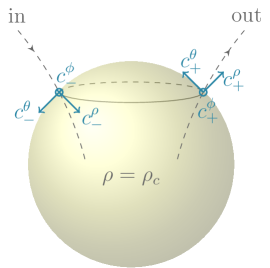
Figure 1: The coordinate light speeds for ingoing and outgoing null rays that pass through a surface of constant radius $\rho_{c}$, i.e., a two-sphere in this example. In an outgoing Bondi-like gauge $c_{+}^{\theta}=0=c_{+}^{\phi}$; i.e., the coordinates $\theta,\phi$ are Lie dragged along the outgoing null ray. This ray is orthogonal to the depicted two-sphere.

III Gauge fixing and the principal symbol

Following closely Khokhlov and Novikov (2002); Hilditch and Richter (2016) we now discuss the structure of the principal symbol of the systems we analyze. See Abalos and Reula (2020); Abalos (2021) for interesting related work on systems with constraints. As shown in Hilditch and Richter (2016), working with the ADM formalism, in this context, one can distinguish among the gauge, constraint and physical variables of the system. This distinction is reflected in the structure of the principal symbol and allows us to understand which gauges can possibly result in SH systems.

FT$2$S Systems and their principal part:

According to Gundlach and Martín-García (2006); Hilditch and Richter (2015) the general first order in time and second in space (FT$2$S) linear constant coefficient system that admits a standard first order reduction is of the form

$$\partial_{t}\mathbf{v} =\mathbfcal{A}_{1}^{i}\partial_{i}\mathbf{v}+\mathbfcal{A}_{1}\mathbf{v}+\mathbfcal{A}_{2}\mathbf{w}+\mathbf{S}_{\mathbf{v}}\,,$$

$$\partial_{t}\mathbf{w} =\mathbfcal{B}_{1}^{ij}\partial_{i}\partial_{j}\mathbf{v}+\mathbfcal{B}_{1}^{i}\partial_{i}\mathbf{v}+\mathbfcal{B}_{1}\mathbf{v}+\mathbfcal{B}_{2}^{i}\partial_{i}\mathbf{w}$$

$$\quad+\mathbfcal{B}_{2}\mathbf{w}+\mathbf{S}_{\mathbf{w}}\,,$$ (24)

where $\mathbf{S}_{\mathbf{v}}$ and $\mathbf{S}_{\mathbf{w}}$ are forcing terms and $\mathbfcal{A}_{1}^{i},\,\mathbfcal{A}_{2},\,\mathbfcal{B}_{1}^{ij},\,\mathbfcal{B}_{2}^{i}$ the principal matrices. In the linear constant coefficient approximation the ADM equations lie in this category. By standard first order reduction we mean one in which all first order derivatives (temporal and spatial) of variables that appear with second order derivatives are introduced as auxiliary variables. We call any first order reduction different from the aforementioned nonstandard. In such a case only a subset of the first order derivatives of a variable that appears up to second order is introduced as auxiliary variables. Or else specific higher derivatives could be. Given an arbitrary unit spatial covector $s_{i}$ (not to be confused with $s_{(\rho)}^{i}$ from the previous section), the principal symbol of the system in the $s_{i}$ direction is defined as

$$\mathbf{P}^{s}=\left(\begin{array}[]{cc}\mathbfcal{A}_{1}^{s}&\mathbfcal{A}_{2}\\ \mathbfcal{B}_{1}^{ss}&\mathbfcal{B}_{2}^{s}\end{array}\right)\,,$$ (27)

where $\mathbfcal{A}_{1}^{s}\equiv\mathbfcal{A}_{1}^{i}s_{i}$ (and so forth). Writing $\mathbf{u}=(\partial_{s}\mathbf{v},\mathbf{w})$, we have

$$\partial_{t}\mathbf{u}\simeq\mathbf{P}^{s}\partial_{s}\mathbf{u}\,,$$ (28)

where here we dropped nonprincipal terms and all derivatives transverse to $s^{i}$. The definitions of weak and strong hyperbolicity are identical to those discussed for first order systems in the Introduction; weak hyperbolicity is the requirement that the eigenvalues of $\mathbf{P}^{s}$ are real for each $s^{i}$, and strong hyperbolicity furthermore is uniformly diagonalizable in $s^{i}$. The second order principal symbol (27) is inherited as a diagonal block of the principal symbol of any standard first order reduction, where the latter furthermore takes an upper block triangular form. Consequently only strongly hyperbolic second order systems may admit a standard first order reduction that is strongly hyperbolic. The importance of this is that (24) has a well-posed initial value problem in the norm

$$E_{1}=\sum_{i}||\partial_{i}\mathbf{v}||_{L^{2}}+||\mathbf{w}||_{L^{2}}\,,$$

if and only if it is strongly hyperbolic, where here the norms are defined over spatial slices of constant $t$. For our analysis, observe that the original characteristic form of the equations of motion is not of the form (24), even after linearization. This issue is overcome by working instead with the ADM equivalent obtained in Sec. II. Working with the equivalent furthermore has the advantage that the theory discussed below was developed in this language, making application straightforward. Due to the freedom in choosing a time slicing, there is freedom in the construction of the equivalent ADM formulation. This was parametrized by $f^{\prime}(\rho)$ in the previous section. For brevity we work assuming $f^{\prime}(\rho)=1$, but since the structural properties discussed above hold true in any alternative slicing, this restriction does not affect the outcome of the analysis.

Pure gauge degrees of freedom:

In many cases of physical interest FT$2$S systems arise with additional structure in their principal symbol. In GR for instance, structure arises as a consequence of gauge freedom. To see this, suppose that we are working in a coordinate basis with an arbitrary solution to the vacuum field equations. The field equations are, of course, invariant under changes of coordinates $x^{\mu}\to X^{\underline{\mu}}$, so that both the metric and curvature transform in the same manner. This invariance has important consequences on the form of the field equations. Consider an infinitesimal change to the coordinates by $x^{\mu}\to x^{\mu}+\xi^{\mu}$. Such a change results in a perturbation to the metric of the form

$$\delta g_{\mu\nu}=-\nabla_{\mu}\xi_{\nu}-\nabla_{\nu}\xi_{\mu}=-\mathcal{L}_{\xi}g_{\mu\nu}\,.$$

This transformation, the linearization of the condition for covariance in a coordinate basis, simultaneously serves as the gauge freedom of linearized GR. Working now in the ADM language, and $3+1$ decomposing $\xi^{a}$ by

$$\Theta\equiv-n_{\mu}\xi^{\mu}\,,\quad\psi^{i}\equiv-\gamma^{i}{}_{\mu}\xi^{\mu}\,,$$

the pure gauge perturbations $(\Theta,\psi^{i})$ satisfy,

$$\partial_{t}\Theta =\delta\alpha-\psi^{i}D_{i}\alpha+\mathcal{L}_{\beta}\Theta\,,$$

$$\partial_{t}\psi^{i} =\delta\beta^{i}+\alpha D^{i}\Theta-\Theta D^{i}\alpha+\mathcal{L}_{\beta}\psi^{i}\,,$$ (29)

with $\delta\alpha$ and $\delta\beta^{i}$ the perturbation of the lapse and shift respectively. The resulting perturbation to the metric and extrinsic curvature can be explicitly computed Hilditch and Richter (2016), and are given by,

$$\delta\gamma_{ij} =-2\Theta K_{ij}+\mathcal{L}_{\psi}\gamma_{ij}\,,$$ (30a)

$$\delta K_{ij} =-D_{i}D_{j}\Theta$$

$$\quad+\Theta\big{(}R_{ij}-2K^{k}{}_{i}K_{jk}+K_{ij}K\big{)}+\mathcal{L}_{\psi}K_{ij}\,,$$ (30b)

where $\gamma_{ij}$ and $K_{ij}$ are to be understood by their background values. It is a remarkable fact that these equations are nothing more than the ADM evolution equations under the replacements $\alpha\to\Theta$ and $\beta^{i}\to\psi^{i}$, so that the ADM evolution equations can be interpreted as a local gauge transformation in a coordinate basis. Given a choice for either the lapse and shift, or an equation of motion for each, or a combination thereof, we may combine (29) and (30), to obtain a closed system for the pure gauge variables $(\Theta,\psi^{i})$ and $(\delta\alpha,\delta\psi^{i}),$ on the background spacetime. We call this the pure gauge subsystem. Suppose, for example, that we employed a harmonic time coordinate ($\Box t=0$) with a vanishing shift. In $3+1$ language this gives

$$\partial_{t}\alpha =-\alpha^{2}K.$$

The pure gauge subsystem (29) for $(\Theta,\psi^{i})$ is then completed by

$$\partial_{t}\delta\alpha \simeq\alpha^{2}\partial^{i}\partial_{i}\Theta\,,\qquad\delta\beta^{i}=0\,,$$

where we have used (30) and discarded nonprincipal terms. The additional structure alluded to above is that for a given choice of gauge, the principal symbol of the pure gauge subsystem is inherited as a sub-block of the principal symbol of any formulation of GR that employs said gauge. This is demonstrated by using suitable projection operators which are stated explicitly below.

Constraint violating degrees of freedom:

Yet more structure arises from the constraints. Assuming the ADM evolution equations hold, the Hamiltonian and momentum constraints formally satisfy evolution equations,

$$\partial_{t}H =-2\alpha D^{i}M_{i}-4M^{i}D_{i}\alpha+2\alpha KH+\mathcal{L}_{\beta}H\,,$$

$$\partial_{t}M_{i} =-\tfrac{1}{2}\alpha D_{i}H+\alpha KM_{i}-D_{i}\alpha H+\mathcal{L}_{\beta}M_{i}\,,$$

so that constraints satisfying initial data remain so in their domain of dependence. These equations follow from the contracted Bianchi identities. In free-evolution formulations of GR however, the ADM evolution equations need not hold, since combinations of the constraints can be freely added to the evolution equations. Doing so results in adjusted evolution equations for the constraints, which nevertheless remain a closed set of equations. Just as the principal symbol of the full equations of motion inherit the pure gauge principal symbol, the principal symbol of the constraint subsystem manifests as a sub-block. This is again seen using the projection operators stated below.

Linearized ADM:

To apply straightforwardly the theory described at the start of this section we linearize about flat space in global inertial coordinates. The analysis can be carried out around a general background leading to the same conclusions. In this setting we obtain for the metric and extrinsic curvature perturbations the evolution equations,

$$\partial_{t}\delta\gamma_{ij} =-2\delta K_{ij}+\partial_{(i}\delta\beta_{j)}\,,$$ (31a)

$$\partial_{t}\delta K_{ij} =-\partial_{i}\partial_{j}\delta\alpha-\tfrac{1}{2}\partial^{k}\partial_{k}\delta\gamma_{ij}$$

$$\quad-\tfrac{1}{2}\partial_{i}\partial_{j}\delta\gamma+\partial^{k}\partial_{(i}\delta\gamma_{j)k}\,.$$ (31b)

The constraints become

$$\delta H =\partial^{i}\partial^{j}\delta\gamma_{ij}-\partial^{i}\partial_{i}\delta\gamma\,,$$

$$\delta M_{i} =\partial^{j}\delta K_{ij}-\partial_{i}\delta K\,,$$

and evolve according to

$$\begin{aligned} \partial_{t}\delta H&=-2\partial^{i}\delta M_{i}\,,\\ \partial_{t}\delta M_{i}&=-\tfrac{1}{2}\partial_{i}\delta H\,.\end{aligned}$$ (32)

About this background the pure gauge equations (29) simplify to

$$\partial_{t}\Theta =\delta\alpha\,,$$ (33a)

$$\partial_{t}\psi_{i} =\delta\beta_{i}+\partial_{i}\Theta\,.$$ (33b)

Pure gauge projection operators:

Let $s^{i}$ be an arbitrary constant spatial unit vector. To extract the gauge, constraint and physical degrees of freedom within the principal symbol in this direction we must decompose the state vector appropriately. The induced metric on the surface transverse to $s^{i}$ is

$$q_{ij}\equiv\gamma_{ij}-s_{i}s_{j}\,.$$

Here we denote by $\hat{A},\,\hat{B}$ the spatial directions transverse to $s^{i}$, which–since in general $s^{i}\neq s_{(\rho)}^{i}$–do not necessarily coincide with the angular directions from our earlier discussion. Projections of the ADM variables that capture pure gauge equations of motion (33) are given by

$$\begin{aligned} &=-\delta K_{ss}\,,\quad[\partial_{s}^{2}\psi_{s}]=\tfrac{1}{2}\partial_{s}\delta\gamma_{ss}\\ [\partial_{s}^{2}\psi_{\hat{A}}]&=\partial_{s}\delta\gamma_{s\hat{A}}\,.\end{aligned}$$ (34)

Here the notation $[\cdots]$ is used to emphasize that the specific projection of the ADM variables on the right-hand side shares, within the principal symbol, the structure of the pure gauge variable named on the left-hand side. This is spelled out below. Thus, together with $\partial_{s}\delta\alpha,\,\partial_{s}\delta\beta_{s},\,\partial_{s}\delta\beta_{\hat{A}}$ they encode the complete pure gauge variables of the system, with $\delta\alpha,\,\delta\beta^{i}$ the perturbation to the lapse and shift.

Constraint projection operators:

Likewise, within the principal symbol the Hamiltonian and momentum constraints are encoded by the projections,

$$\begin{aligned} &=-\partial_{s}\delta\gamma_{qq}\,,\quad[M_{s}]=-\delta K_{qq}\,,\\ [M_{\hat{A}}]&=\delta K_{s\hat{A}}\,,\end{aligned}$$ (35)

with the naming convention as above. Here and in the following indices $qq$ denote that the trace was taken with $q^{ij}$.

Physical projection operators:

Finally, the remaining variables to be taken account of are the trace-free projections. Defining the projection operator familiar from textbook treatments of linear gravitational waves,

$${}^{P}\!\!\!\perp^{kl}_{ij}\equiv q^{k}_{\;(i}q^{l}{}_{j)}-\tfrac{1}{2}q_{ij}q^{kl}\,.$$ (36)

we define

$$\begin{aligned} \partial_{s}\delta\gamma_{\hat{A}\hat{B}}^{\textrm{TF}}&={}^{P}\!\!\!\perp^{ij}_{\hat{A}\hat{B}}\partial_{s}\delta\gamma_{ij}\,,\quad\delta K_{\hat{A}\hat{B}}^{\textrm{TF}}={}^{P}\!\!\!\perp^{ij}_{\hat{A}\hat{B}}\delta K_{ij}\,.\end{aligned}$$

The superscript TF denotes trace-free. These variables are associated with the physical degrees of freedom.

The principal symbol:

Employing the notation above we can now write out the principal symbol in the form (28). Starting with the pure gauge block, this gives

$$\begin{aligned} \partial_{t}[\partial_{s}^{2}\Theta]&\simeq\partial_{s}(\partial_{s}\delta\alpha)+\tfrac{1}{2}\partial_{s}[H]\,,\\ \partial_{t}[\partial_{s}^{2}\psi_{s}]&\simeq\partial_{s}(\partial_{s}\delta\beta_{s})+\partial_{s}[\partial_{s}^{2}\Theta]\,,\\ \partial_{t}[\partial_{s}^{2}\psi_{\hat{A}}]&\simeq\partial_{s}(\partial_{s}\delta\beta_{\hat{A}})-2\partial_{s}[M_{\hat{A}}]\,.\end{aligned}$$ (37)

Comparing this with (33) it is clear that up to additions of the “constraint variables” there is agreement. Next, the constraint violating block gives

$$\begin{aligned} \partial_{t}[H]&\simeq-2\partial_{s}[M_{s}]\,,\\ \partial_{t}[M_{s}]&\simeq-\tfrac{1}{2}\partial_{s}[H]\,,\\ \partial_{t}[M_{\hat{A}}]&\simeq 0\,.\end{aligned}$$ (38)

Comparing this with (32) there is perfect agreement. Finally the physical block is

$$\begin{aligned} \partial_{t}\partial_{s}\delta\gamma_{\hat{A}\hat{B}}^{\textrm{TF}}&\simeq-2\partial_{s}\delta K_{\hat{A}\hat{B}}^{\textrm{TF}}\,,\\ \partial_{t}\delta K_{\hat{A}\hat{B}}^{\textrm{TF}}&\simeq-\tfrac{1}{2}\partial_{s}^{2}\delta\gamma_{\hat{A}\hat{B}}^{\textrm{TF}}\,,\end{aligned}$$ (39)

which is decoupled from the rest of the equations. These equations are not yet complete, because we have not yet made a concrete choice of gauge. Several Bondi-like gauges are treated in detail in the following sections.

Discussion:

The results of the foregoing discussion follow because GR is a constrained Hamiltonian system that satisfies the hypotheses of Hilditch and Richter (2016). To make the presentation here somewhat more stand-alone however, let us consider a plane wave ansatz

$$\begin{aligned} \delta\gamma_{ij}&=2e^{\kappa^{(\psi_{s})}_{\mu}x^{\mu}}s_{i}s_{j}[\partial_{s}\tilde{\psi_{s}}]-\tfrac{1}{2}q_{ij}e^{\kappa^{(H)}_{\mu}x^{\mu}}[\tilde{H}]\\ &+2e^{\kappa^{(\psi_{A})}_{\mu}x^{\mu}}q^{\hat{A}}{}_{(i}s_{j)}[\partial_{s}\tilde{\psi}_{\hat{A}}]+e^{\kappa^{(P)}_{\mu}x^{\mu}}{}^{P}\!\!\!\perp^{\hat{A}\hat{B}}_{ij}\delta\gamma_{\hat{A}\hat{B}}^{\textrm{TF}}\,,\\ \delta K_{ij}&=-e^{\kappa^{(\Theta)}_{\mu}x^{\mu}}s_{i}s_{j}[\partial^{2}_{s}\tilde{\Theta}]-\tfrac{1}{2}q_{ij}e^{\kappa^{(M_{s})}_{\mu}x^{\mu}}[\tilde{M}_{s}]\\ &+2e^{\kappa^{(M_{A})}_{\mu}x^{\mu}}q^{\hat{A}}{}_{(i}s_{j)}[\tilde{M}_{\hat{A}}]+e^{\kappa^{(P)}_{\mu}x^{\mu}}{}^{P}\!\!\!\perp^{\hat{A}\hat{B}}_{ij}\delta K_{\hat{A}\hat{B}}^{\textrm{TF}}\,,\end{aligned}$$ (40)

with each wave vector of the form $\kappa_{\mu}=(\kappa,i\,\omega s_{i})$. These solutions travel in the $\pm s^{i}$ directions, although since the lapse and shift are as yet undetermined, the $\kappa$’s cannot be solved for so far. Defining the projections exactly as above, the unknowns can be decomposed explicitly into their gauge, constraint violating and gravitational wave pieces as indicated by the naming, and Eqs. (37), (38), and (39) become exact. In the nonlinear setting it is, of course, hopeless to try and decompose metric components into constituent gauge, constraint violating and physical degrees of freedom. But even in the linear constant coefficient approximation, solutions consist in general of a sum over many such plane waves propagating in different directions, and so the decomposition (40) is not a sufficient description. What is important for our purposes however, is that the structure in the field equations that permits the decomposition (40) for plane wave solutions is present regardless of the direction $s^{i}$ considered. The principal symbol sees only this structure and thus, with Eqs. (37), (38) and (39) above completed with a choice for the lapse and shift, can be written in the schematic form

$$\mathbf{P}^{s}=\begin{pmatrix}\mathbf{P}_{G}&\mathbf{P}_{GP}&\mathbf{P}_{GC}\\ 0&\mathbf{P}_{P}&\mathbf{P}_{PC}\\ 0&0&\mathbf{P}_{C}\end{pmatrix}\,,$$ (41)

even upon linearization about an arbitrary background. Here $\mathbf{P}_{G},\,\mathbf{P}_{C},\,\mathbf{P}_{P}$ denote the gauge, constraint and physical sub-blocks and $\mathbf{P}_{GC},\,\mathbf{P}_{GP},\,\mathbf{P}_{PC}$ parametrize the coupling between them. As seen in Hilditch and Richter (2016) there is a very large class of gauge conditions and natural constraint additions that result in $\mathbf{P}_{GP}=\mathbf{P}_{GC}=\mathbf{P}_{PC}=0$. Consequently, it follows from (41) that a necessary condition for strong hyperbolicity of the formulation is that the pure gauge and constraint subsystems are themselves strongly hyperbolic. Following Khokhlov and Novikov (2002) we may therefore restrict our attention first to pure gauge systems of interest, which have the advantage of being smaller, and thus are much easier to treat.

Bondi-like gauges:

The gauges we are concerned with all require the condition (2), which in characteristic coordinates implies the same for the perturbation to the metric, that is,

$$\delta g^{uu}=\delta g^{uA}=0\,.$$

There remains one gauge condition to be specified, namely the parametrization along outgoing null surfaces by a radial coordinate. Next we study specific instances of this condition.

IV The affine null gauge

In this section we analyze the degree of hyperbolicity of the EFE in the affine null gauge Winicour (2013); Crespo et al. (2019). In Giannakopoulos et al. (2020) a hyperbolicity analysis for the EFE in the affine null gauge for asymptotically AdS five-dimensional spacetime with planar symmetry was performed and the full system was shown to be WH. Here, we do this analysis in four-dimensional asymptotically flat spacetime, but more importantly we also analyze the pure gauge subsystem and show that the weak hyperbolicity of the full system stems from that of the pure gauge subsystem.

The complete affine null gauge fixing is given by

$$\alpha=L^{-1}\,,\quad\beta^{\rho}=L^{-2}-1\,,\quad\beta^{A}=-b^{A}L^{-2}\,,$$ (42)

where Eqs. (21) -(23) and $g^{ur}=-1$ have been combined. As in the previous section, we work in the linear, constant coefficient approximation, and for simplicity we assume that in (5) $f(\rho)=\rho$.

IV.1 Pure gauge subsystem

Let us first consider pure gauge metric perturbations (30). To close the system (33) further input for $\delta\alpha$ and $\delta\beta^{i}$ is needed. For the affine null gauge this follows from (42), which after linearization about flat space reads

$$\delta\alpha =-\tfrac{1}{2}\delta\gamma_{\rho\rho}\,,\quad\;\delta\beta^{\theta}=-\rho^{-2}\delta\gamma_{\rho\theta}\,,$$

$$\delta\beta^{\rho} =-\delta\gamma_{\rho\rho}\,,\qquad\delta\beta^{\phi}=-\rho^{-2}\sin^{2}\theta\,\delta\gamma_{\rho\phi}\,.$$

Using $\delta\gamma_{ij}=\partial_{i}\psi_{j}+\partial_{j}\psi_{i}$ and $\psi^{i}=\gamma^{ij}\psi_{j}$ the latter reads

$$\delta\alpha =-\partial_{\rho}\psi^{\rho}\,,\quad\,\delta\beta^{\theta}=-\partial_{\rho}\psi^{\theta}-\rho^{-2}\partial_{\theta}\psi^{\rho}\,,$$ (43)

$$\delta\beta^{\rho} =-2\partial_{\rho}\psi^{\rho}\,,\;\;\delta\beta^{\phi}=-\partial_{\rho}\psi^{\phi}-\rho^{-2}\sin^{2}\theta\,\partial_{\phi}\psi^{\rho}\,.$$

The pure gauge subsystem (33) is then

$$(\partial_{t}+\partial_{\rho})(\psi^{\rho}-\Theta)=0\,,$$ (44a)

$$(\partial_{t}+\partial_{\rho})\psi^{\rho}+\partial_{\rho}(\psi^{\rho}-\Theta)=0\,,$$ (44b)

$$(\partial_{t}+\partial_{\rho})\psi^{\theta}+\rho^{-2}\partial_{\theta}(\psi^{\rho}-\Theta)=0\,,$$ (44c)

$$(\partial_{t}+\partial_{\rho})\psi^{\phi}+(\rho\sin\theta)^{-2}\partial_{\phi}(\psi^{\rho}-\Theta)=0\,,$$ (44d)

where $\partial_{t}+\partial_{\rho}=\partial_{r}$ is an outgoing null derivative and (44a) results from a linear combination of (33a) and (33b) with $i=\rho$. Along an arbitrary spatial direction $s^{i}$ a first order linear system can be written as

$$\partial_{t}\mathbf{v}\simeq\mathbf{J}^{s}\partial_{s}\mathbf{v}\,,$$

where $\mathbf{T}^{-1}_{s}\mathbf{P}^{s}\mathbf{T}_{s}\equiv\mathbf{J}^{s}$ is the Jordan normal form of the principal symbol, $\mathbf{P}^{s}$, $\mathbf{v}\equiv\mathbf{T}^{-1}_{s}\mathbf{u}$ are the associated (generalized) characteristic variables and $\simeq$ denotes equality up to source terms and derivatives transverse to $s^{i}$. The principal symbol of the pure gauge subsystem (44) is clearly nondiagonalizable along the $\rho,\theta,\phi$ directions, and, in fact, in any direction. In (44b), (44c), and (44d) the terms $\partial_{\rho}(\psi^{\rho}-\Theta)$, $\partial_{\theta}(\psi^{\rho}-\Theta)$, and $\partial_{\phi}(\psi^{\rho}-\Theta)$ result in $2\times 2$ Jordan blocks, along $\rho,\theta$, and $\phi$, respectively. The principal symbol of the full set of equations of motion for GR has the upper triangular form (41) when a standard first order reduction is considered. Thus it will possess nontrivial Jordan blocks along all $\rho,\theta,\phi$ directions as well. In Secs. IV.2 and IV.3 we show this explicitly and demonstrate the connection to the PDE system in characteristic coordinates.

An intriguing observation is that the pure gauge variable $(\psi^{\rho}-\Theta)$ satisfies a transport equation along $\partial_{r}$. So, acting from the left on (44) with $\partial_{r}$ and commuting the spatial and null derivatives on $(\psi^{\rho}-\Theta)$, one obtains

$$\partial_{r}^{2}(\Theta-\psi^{\rho})=0\,,$$ (45a)

$$\partial_{r}^{2}\psi^{\rho}=0\,,$$ (45b)

$$\partial_{r}^{2}\psi^{\theta}=0\,,$$ (45c)

$$\partial_{r}^{2}\psi^{\phi}=0\,.$$ (45d)

This system admits a nonstandard reduction to first order which is strongly hyperbolic. To see this, we introduce only outgoing null derivatives of the unknowns as auxiliary variables. All of the variables then satisfy transport equations in the outgoing null direction. In contrast to this, for a standard first order reduction both the time and space derivatives of the unknowns would be introduced as auxiliary variables.

The relevant question is whether there exists a formulation of GR that inherits the structure of the second version of the pure gauge subsystem (45), rather than the first (44). In view of the results of Hilditch and Richter (2016), if such a formulation exists, it would necessarily admit a nonstandard first order reduction. In Sec. IV.2 we show that there is a convenient combination of ADM variables that allows one to remove the nontrivial Jordan block along the $\rho$ direction that appears in a standard first order reduction. This is true due to the specific gauge choice and its construction upon outgoing null geodesics. Crucially, however, this special combination is only possible along the $\rho$ direction but not $\theta,\phi$. So, away from spherical symmetry the EFE in the affine null gauge are only WH.

IV.2 Pure gauge sub-block: Radial direction

We now demonstrate how the radial part of the pure gauge subsystem (44) is inherited by the linearized EFE. For brevity in this subsection we work in spherical symmetry, which is sufficient, since the coupled gauge variables in the radial Jordan block of (44) are present already under this assumption.

IV.2.1 ADM setup

In spherical symmetry the principal part of the linearized ADM equations in outgoing affine null gauge is

$$\partial_{t}\delta\gamma_{\rho\rho} \simeq-2\delta K_{\rho\rho}-2\partial_{\rho}\delta\gamma_{\rho\rho}\,,$$ (46a)

$$\partial_{t}\delta K_{\rho\rho} \simeq\tfrac{1}{2}\partial_{\rho}^{2}\delta\gamma_{\rho\rho}-\rho^{-2}\partial_{\rho}^{2}\delta\gamma_{\theta\theta}\,,$$ (46b)

$$\partial_{t}\delta\gamma_{\theta\theta} \simeq-2\delta K_{\theta\theta}\,,$$ (46c)

$$\partial_{t}\delta K_{\theta\theta} \simeq-\tfrac{1}{2}\partial_{\rho}^{2}\delta\gamma_{\theta\theta}\,.$$ (46d)

From Eq. (34), the gauge variables along the $\rho$ direction in spherical symmetry are

$$-\delta K_{\rho\rho}=[\partial_{\rho}^{2}\Theta]\,,\qquad\tfrac{1}{2}\partial_{\rho}\delta\gamma_{\rho\rho}=[\partial_{\rho}^{2}\psi^{\rho}]\,.$$ (47)

To recover the pure gauge structure it suffices to analyze the coupling between (46a) and (46b),

$$\partial_{r}(\tfrac{1}{2}\delta\gamma_{\rho\rho}) \simeq-\delta K_{\rho\rho}-\partial_{\rho}(\tfrac{1}{2}\delta\gamma_{\rho\rho})\,,$$ (48a)

$$\partial_{r}(\delta K_{\rho\rho}+\tfrac{1}{2}\partial_{\rho}\delta\gamma_{\rho\rho}) \simeq-\rho^{-2}\partial_{\rho}^{2}\delta\gamma_{\theta\theta}\,,$$ (48b)

where $\partial_{r}=\partial_{t}+\partial_{\rho}$ is an outgoing null vector and (48b) results from a linear combination of (46a) and (46b). The right-hand side of (48b) involves the constraint variable

$$[H]=-\partial_{\rho}\delta\gamma_{qq}=-2\rho^{-2}\partial_{\rho}\delta\gamma_{\theta\theta}\,.$$

In a standard first order reduction, the term $(\partial_{\rho}\delta\gamma_{\rho\rho})$ would be introduced as an evolved variable satisfying

$$\partial_{r}(\tfrac{1}{2}\partial_{\rho}\delta\gamma_{\rho\rho}) \simeq-\partial_{\rho}\delta K_{\rho\rho}-\partial_{\rho}(\tfrac{1}{2}\partial_{\rho}\delta\gamma_{\rho\rho})\,.$$ (49)

The above and (48b) expressed in terms of gauge and constraint variables read

$$\partial_{r}[\partial_{\rho}^{2}\psi^{\rho}]+\partial_{\rho}[\partial_{\rho}^{2}\left(\psi^{\rho}-\Theta\right)]\simeq 0\,,$$

$$\partial_{r}[\partial_{\rho}^{2}\left(\Theta-\psi^{\rho}\right)]\simeq\tfrac{1}{2}\partial_{\rho}[H]\,.$$

As explained in Sec. III, this system has a pure gauge part that consists of the coupling among the gauge variables $\Theta$ and $\psi^{\rho}$ and a part that captures the coupling of the gauge to the constraint variables. The pure gauge part $\mathbf{P}_{G}$ is obtained by neglecting the term $\partial_{\rho}[H]/2$. This part has the same principal structure as the pure gauge subsystem (44) in the radial direction, since it is just an overall $\partial_{\rho}^{2}$ derivative of the latter. This is in accordance with the result of Hilditch and Richter (2016), because for a standard first order reduction $\mathbf{P}_{G}$ inherits the structure of the first order system formed by $(\Theta,\psi_{i},\delta\alpha,\delta\beta_{i})$. The term $\partial_{\rho}[H]/2$ is encoded in the $\mathbf{P}_{GC}$ sub-block of the full principal symbol $\mathbf{P}^{\rho}$.

Next, let us consider a reduction in which $(\partial_{r}\delta\gamma_{\rho\rho})$ is introduced as an auxiliary variable rather than $(\partial_{\rho}\delta\gamma_{\rho\rho})$. From (48a) and (47) we get

$$\partial_{r}(\tfrac{1}{2}\delta\gamma_{\rho\rho})=[\partial_{r}\partial_{\rho}\psi^{\rho}]\simeq[\partial_{\rho}^{2}(\Theta-\psi^{\rho})]\,,$$ (50)

where in the first step we are just using our normal naming convention with $[\dots]$ and likewise in the second Eq. (47). Similarly, from Eq. (47) we get

$$\tfrac{1}{2}\partial_{\rho}\delta\gamma_{\rho\rho}+\delta K_{\rho\rho}=[\partial_{\rho}^{2}(\psi^{\rho}-\Theta)]=[\partial_{r}\partial_{\rho}\psi^{\rho}]=-[\partial_{r}\partial_{\rho}\Theta]\,,$$ (51)

where in the second step Eq. (44b) and in the third Eq. (44a) are used. The equation of motion for the auxiliary variable $(\partial_{r}\delta\gamma_{\rho\rho})$ results from (48a) after acting with $\partial_{r}$, namely

$$\partial_{r}(\tfrac{1}{2}\partial_{r}\delta\gamma_{\rho\rho}) \simeq-\partial_{r}(\delta K_{\rho\rho}+\tfrac{1}{2}\partial_{\rho}\delta\gamma_{\rho\rho})$$

$$\simeq\rho^{-2}\partial_{\rho}^{2}\delta\gamma_{\theta\theta}\,,$$ (52)

where in the second step Eq. (48b) is used. The above together with Eq. (48b) in terms of the gauge and constraint variables read

$$\partial_{r}[\partial_{r}\partial_{\rho}\psi^{\rho}] \simeq-\tfrac{1}{2}\partial_{\rho}[H]\,,$$ (53a)

$$\partial_{r}[\partial_{r}\partial_{\rho}\Theta] \simeq\tfrac{1}{2}\partial_{\rho}[H]\,,$$ (53b)

where the relations (50) and (51) have been used. Thus, the system (48b) and (52) inherits the principal structure of (45a) and (45b) in $\mathbf{P}_{G}$. Again the term $\partial_{\rho}[H]/2$ is in the $\mathbf{P}_{GC}$ sub-block. This result does not contradict Hilditch and Richter (2016) due to the nonstandard first order reduction considered. In the outgoing affine null gauge the outgoing null direction possesses a special role as the foundational piece of the construction. This construction provides the opportunity to group ADM variables in such a way that we can avoid the nontrivial Jordan block in the radial direction.

IV.2.2 Characteristic setup

The ADM analysis above teaches us which variables inherit the principal structure of the pure gauge degrees of freedom. However, the original PDE problem is formulated in the characteristic domain. In Hilditch and Richter (2016) the pure gauge structure was identified for a spacelike foliation. Whether this is possible in the characteristic domain is closely related to the existence of the previous first order reductions in this domain as well. We show here that both previous first order reductions and their principal structure can be realized in the characteristic setup directly.

To demonstrate this consider the affine null gauge in an outgoing characteristic formulation. The complete calculation can be found in the ancillary files. We first employ the metric ansatz

$$ds^{2}=g_{uu}du^{2}-2dudr+g_{\theta\theta}d\theta^{2}+g_{\phi\phi}d\phi^{2}\,,$$

which for flat space reads

$$g_{uu}=-1\,,\quad g_{\theta\theta}=r^{2}\,,\quad g_{\phi\phi}=r^{2}\sin^{2}\theta\,.$$

Analyzing the main equations $R_{rr}=R_{\theta\theta}=R_{\phi\phi}=0$ linearized about flat space we see the following structure

$$\partial_{r}\delta g_{uu}-\frac{1}{2\rho}\partial_{\rho}\left(\partial_{r}\delta g_{\theta\theta}+\sin^{-2}\theta\partial_{r}\delta g_{\phi\phi}\right)=0\,,$$ (54a)

$$\partial_{r}\left(\partial_{r}\delta g_{\theta\theta}+\sin^{-2}\theta\partial_{r}\delta g_{\phi\phi}\right)=0\,.$$ (54b)

The variable $\left(\partial_{r}\delta g_{\theta\theta}+\sin^{-2}\theta\partial_{r}\delta g_{\phi\phi}\right)$ in (54a) prevents $\delta g_{uu}$ from satisfying just an advection equation along $\partial_{r}$ and so provides a nontrivial Jordan block. The combination of $\delta g_{\theta\theta}$ and $\delta g_{\phi\phi}$ in the former hints that a different choice of variables may be more appropriate. This combination of variables furthermore appears in the trivial equation $R_{ur}=0$ when linearized about flat space, and so it may be optimal to group them together. We thus next consider the equations as resulting from the metric ansatz

$$ds^{2}=g_{uu}du^{2}-2dudr+\hat{R}(u,r)^{2}\left(d\theta^{2}+\sin^{2}\theta d\phi^{2}\right)\,,$$

where $\hat{R}$ is the radius of the two-sphere. This form of the metric ansatz is used in the spherically symmetric case of Winicour (2013), employed by Crespo et al. (2019) in the study of gravitational collapse of a massless scalar field, as well as in van der Walt and Bishop (2012) for cosmological considerations using past null cones. Upon linearization about flat space the characteristic PDE system takes the form

$$\partial_{r}^{2}\delta\hat{R}=0\,,$$ (55a)

$$2r\partial_{u}\partial_{r}\delta\hat{R}+2\partial_{u}\delta\hat{R}$$

$$\quad-2\partial_{r}\delta\hat{R}+r\partial_{r}\delta g_{uu}+\delta g_{uu}=0\,,$$ (55b)

$$4\partial_{u}\partial_{r}\delta\hat{R}+r\partial_{r}^{2}\delta g_{uu}+2\partial_{r}\delta g_{uu}=0\,.$$ (55c)

Equations (55a) and (55b) correspond to the main equations $R_{rr}=0$ and $R_{\theta\theta}=0$, respectively, and Eq. (55c) to the trivial one $R_{ur}=0$. The main equation $R_{\phi\phi}$ is dropped since it is proportional to $R_{\theta\theta}$ and the two-sphere is parametrized only by its radius.

Comparing once more with the ADM form of the problem, including in the system the trivial equation (55c) corresponds to including in the analysis the linearized ADM equation for $\delta K_{\rho\rho}$. This is an essential component in identifying the pure gauge sub-block along the radial direction. To achieve this we first make the following identification using Eq. (8):

$$g_{uu}=\alpha^{-2}-2\,,$$

which after linearization about flat space yields

$$\delta g_{uu}=-2\delta\alpha=\delta\gamma_{\rho\rho}\,,$$ (56)

where the gauge condition $\delta\alpha=-\delta\gamma_{\rho\rho}/2$ is used. We consider now a first order reduction with

$$(\partial_{r}\delta\hat{R})\,,\quad(\partial_{u}\delta\hat{R})\,,\quad(\partial_{r}\delta g_{uu})$$

promoted to independent variables where, by (56), the latter is equivalent to $(\partial_{r}\delta\gamma_{\rho\rho})$ being treated as a reduction variable. This first order reduction provides a diagonalizable radial principal part for (55) with advection equations along $\partial_{r}$ for all variables–original and auxiliary–and corresponds to the pure gauge subsystem (45). More precisely, the relation between the ADM gauge variables and the characteristic variables is

$$\tfrac{1}{2}\partial_{\rho}\delta\gamma_{\rho\rho} =\tfrac{1}{2}(\partial_{r}\delta g_{uu}-\partial_{u}\delta g_{uu})\,,$$ (57a)

$$-\delta K_{\rho\rho} =\partial_{r}\delta g_{uu}-\tfrac{1}{2}\partial_{u}\delta g_{uu}\,.$$ (57b)

Since all characteristic variables satisfy advection equations along $\partial_{r}$, combining (57) with (50) and (51) one recovers (53).

If $(\partial_{u}\delta g_{uu})$ is also taken as an auxiliary variable, then the first order reduction is of the standard type, since

$$\partial_{\rho}\delta g_{uu}=\partial_{r}\delta g_{uu}-\partial_{u}\delta g_{uu}\,.$$

The equation of motion for $(\partial_{u}\delta g_{uu})$ can be obtained from

$$\partial_{r}(\partial_{u}\delta g_{uu})=\partial_{u}(\partial_{r}\delta g_{uu})\,.$$

This first order reduction of (55) possesses the following nontrivial Jordan block

$$(\partial_{t}+\partial_{\rho})(\partial_{u}\delta g_{uu})+\partial_{\rho}(\partial_{r}\delta g_{uu})=0\,,$$

$$(\partial_{t}+\partial_{\rho})(\partial_{r}\delta g_{uu})=0\,,$$

and a linear combination yields

$$(\partial_{t}+\partial_{\rho})\left[(\partial_{r}\delta g_{uu})-(\partial_{u}\delta g_{uu})\right]=\partial_{\rho}(\partial_{r}\delta g_{uu})\,.$$

Via the identification (57) the latter matches (49), modulo an overall factor of $1/2$. Hence, the Jordan block of the characteristic PDE with this characteristic standard first order reduction coincides precisely with the pure gauge principal part (44a) and (44b). This is merely the characteristic version of the standard first order reduction in the Cauchy frame. The alternative choice, where, instead of introducing both $(\partial_{u}\delta g_{uu})$ and $(\partial_{r}\delta g_{uu})$ as auxiliary variables, only the latter is introduced, renders the characteristic PDE system in spherical symmetry strongly hyperbolic. Consequently, the initial value problem of this system is not well-posed in a norm where both $(\partial_{t}\delta g_{uu})^{2}$ and $(\partial_{\rho}\delta g_{uu})^{2}$ are included in the integrand, but in one that involves only $(\partial_{r}\delta g_{uu})^{2}$. Based on this norm, one can study well-posedness of the CIBVP of the system by seeking energy estimates, similar to the analysis of Giannakopoulos et al. (2020). See also Balean (1997) for energy estimates of the wave and Maxwell equations in a single-null characteristic setup.

IV.3 Pure gauge sub-block: Angular direction $\theta$

We next expand the previous analysis to a setup without symmetry, focusing purely on the angular direction $\theta$. The pure gauge structure is identified in both the ADM and characteristic setups. In contrast, however, to the radial direction there is no combination of variables that allows us to avoid the nontrivial Jordan block of the pure gauge. We also discuss which choice of variables is most convenient for the analysis.

IV.3.1 ADM setup

The partition in to gauge, constraint, and physical variables along the $\theta$ direction is still achieved using Eqs. (34), (35), and (36), respectively. The gauge variables are

$$=-\delta K_{\theta\theta}\,,\quad\quad\;\;[\partial_{\theta}^{2}\psi^{\rho}]=\partial_{\theta}\delta\gamma_{\rho\theta}\,,$$ (58)

$$[\partial_{\theta}^{2}\psi^{\theta}] =\frac{1}{2\rho^{2}}\partial_{\theta}\delta\gamma_{\theta\theta}\,,\quad[\partial_{\theta}^{2}\psi^{\phi}]=\frac{1}{\rho^{2}\sin^{2}\theta}\partial_{\theta}\delta\gamma_{\theta\phi}\,.$$

The constraint variables are

$$[H]=-\partial_{\theta}\delta\gamma_{\rho\rho}-\frac{1}{\rho^{2}\sin^{2}\theta}\partial_{\theta}\delta\gamma_{\phi\phi}\,,\quad[M_{\rho}]=\delta K_{\rho\theta}\,,$$ (59)

$$\!\![M_{\theta}]=-\delta K_{\rho\rho}-\frac{1}{\rho^{2}\sin^{2}\theta}\delta K_{\phi\phi}\,,\qquad[M_{\phi}]=\delta K_{\theta\phi}\,.$$

The physical variables are obtained with the action of ${}^{P}\!\!\!\perp$ on $\delta\gamma_{ij}$ and $\delta K_{ij}$. As seen from the physical subsystem (39), the latter is essentially a time derivative of the former. We work with the physical variables

$$[h_{+}] \equiv\frac{1}{2}\delta\gamma_{\rho\rho}-\frac{1}{2\rho^{2}\sin^{2}\theta}\delta\gamma_{\phi\phi}\,,\quad[h_{\times}]\equiv\delta\gamma_{\rho\phi}\,,$$ (60a)

$$[\dot{h}_{+}] \equiv\frac{1}{\rho^{2}\sin^{2}\theta}\delta K_{\phi\phi}-\delta K_{\rho\rho}\,,\quad[\dot{h}_{\times}]\equiv-2\delta K_{\rho\phi}\,,$$ (60b)

which correspond to the two polarizations of the gravitational waves in GR. In Eq. (60b) we have multiplied with an overall factor of $-2$ for the definitions to be compatible with the physical subsystem (39) when $[\dot{h}_{+}]=\partial_{t}h_{+}$, and similarly for $[h_{\times}]$. As expected for a gravitational wave that travels along the $\theta$ direction, the physical variables involve only spatial metric components that are transverse to this direction. The principal symbol in the form (28) in the $\theta$ direction for the linearized ADM formulation is

$$\partial_{t}\delta\gamma_{\rho\rho} \simeq-2\delta K_{\rho\rho}\,,$$ (61a)

$$\partial_{t}\delta\gamma_{\rho\theta} \simeq-2\delta K_{\rho\theta}-\partial_{\theta}\delta\gamma_{\rho\rho}\,,$$ (61b)

$$\partial_{t}\delta\gamma_{\rho\phi} \simeq-2\delta K_{\rho\phi}\,,$$ (61c)

$$\partial_{t}\delta\gamma_{\theta\theta} \simeq-2\delta K_{\theta\theta}-2\partial_{\theta}\delta\gamma_{\rho\theta}\,,$$ (61d)

$$\partial_{t}\delta\gamma_{\theta\phi} \simeq-2\delta K_{\theta\phi}-\partial_{\theta}\delta\gamma_{\rho\phi}\,,$$ (61e)

$$\partial_{t}\delta\gamma_{\phi\phi} \simeq-2\delta K_{\phi\phi}\,,$$ (61f)

and

$$\partial_{t}\delta K_{\rho\rho} \simeq-\frac{1}{2\rho^{2}}\partial_{\theta}^{2}\delta\gamma_{\rho\rho}\,,$$ (62a)

$$\partial_{t}\delta K_{\rho\theta} \simeq 0\,,$$ (62b)

$$\partial_{t}\delta K_{\rho\phi} \simeq-\frac{1}{2\rho^{2}}\partial_{\theta}^{2}\delta\gamma_{\rho\phi}\,,$$ (62c)

$$\partial_{t}\delta K_{\theta\theta} \simeq-\frac{1}{2\rho^{2}\sin^{2}\theta}\partial_{\theta}^{2}\delta\gamma_{\phi\phi}\,,$$ (62d)

$$\partial_{t}\delta K_{\theta\phi} \simeq 0\,,$$ (62e)

$$\partial_{t}\delta K_{\phi\phi} \simeq-\frac{1}{2\rho^{2}}\partial_{\theta}^{2}\delta\gamma_{\phi\phi}\,.$$ (62f)

For a standard first order reduction the pure gauge principal structure along the $\theta$ direction is inherited by

$$\partial_{t}(\tfrac{1}{2\rho^{2}}\partial_{\theta}\delta\gamma_{\theta\theta}) \simeq-\rho^{-2}\partial_{\theta}\left(\partial_{\theta}\delta\gamma_{\rho\theta}+\delta K_{\theta\theta}\right)\,,$$ (63a)

$$\partial_{t}\left(\partial_{\theta}\delta\gamma_{\rho\theta}+\delta K_{\theta\theta}\right) \simeq-\partial_{\theta}^{2}\delta\gamma_{\rho\rho}-\tfrac{1}{2\rho^{2}\sin^{2}\theta}\partial_{\theta}^{2}\delta\gamma_{\phi\phi}$$

$$\quad-2\partial_{\theta}\delta K_{\rho\theta}\,.$$ (63b)

After using Eqs.(58), (59), and (60) the system (63) yields

$$\partial_{t}[\partial_{\theta}^{2}\psi^{\theta}]+\rho^{-2}\partial_{\theta}[\partial_{\theta}^{2}\left(\psi^{\rho}-\Theta\right)]\simeq 0\,,$$ (64)

$$\partial_{t}[\partial_{\theta}^{2}\left(\psi^{\rho}-\Theta\right)]\simeq\tfrac{3}{4}\partial_{\theta}[H]-2\partial_{\theta}[M_{\theta}]-\tfrac{1}{2}\partial_{\theta}^{2}[h_{+}]\,,$$

so that, comparing with (44), the pure gauge structure of $\mathbf{P}_{G}$ is manifest within the full principal symbol, as too is the coupling among gauge, constraint, and physical variables encoded in $\mathbf{P}_{GC}$ and $\mathbf{P}_{GP}$. Here we have worked with the plain ADM evolution equations. Working with the ADM equivalent discussed in Sec. II changes only the coupling to the constraints. To obtain this result the necessary conditions were

1. Introduction of the quantities $(\partial_{\theta}\delta\gamma_{\theta\theta})$ and $(\partial_{\theta}\delta\gamma_{\rho\theta})$ as auxiliary variables.

2. Inclusion of the equation of motion for $\delta K_{\theta\theta}$ in the analyzed system.

Interestingly, the affine null gauge provides an explicit example where the sub-block $\mathbf{P}_{GP}$ of the full principal symbol $\mathbf{P}^{s}$ is nonvanishing, so there is nontrivial coupling between gauge and physical variables in the principal symbol.

IV.3.2 Characteristic setup

We repeat now the previous analysis directly in the characteristic coordinates and variables to demonstrate how the pure gauge structure is inherited in $\mathbf{P}^{\theta}$ for the characteristic setup. The ADM analysis is again used as guidance in this. More specifically, from the equivalent ADM system (14) we know that the characteristic system involves the equation of motion for $\delta K_{\theta\theta}$, which is one of the two necessary conditions in order to recover the structure we are looking for. We parametrize the metric functions simply by  $g_{uu},\,g_{u\theta},\,g_{u\phi},\,g_{\theta\theta},\,g_{\phi\theta},\,g_{\phi\phi}$. For the present calculations this choice, as opposed to that of Winicour (2013), is preferred due to its cleaner connection to the ADM variables and allows us to uncover the pure gauge structure more easily.

With this parametrization the PDE system consisting of the main equations (3) does not involve terms of the form $\partial_{\theta}^{2}\delta g_{u\theta}$ and $\partial_{\theta}^{2}\delta g_{\theta\theta}$, which in the ADM language correspond to $\partial_{\theta}^{2}\delta\gamma_{\rho\theta}$ and $\partial_{\theta}^{2}\delta\gamma_{\theta\theta}$. A minimal first order reduction of the characteristic system, the details of which can be found in the ancillary files, exhibits the following Jordan block in the $\theta$ direction:

$$\partial_{t}\delta g_{uu}+\frac{1}{2\rho\sin^{2}\theta}\partial_{t}(\partial_{r}\delta g_{\theta\theta})$$

$$\qquad\quad-\frac{1}{\rho^{2}}\partial_{\theta}\delta g_{u\theta}+\frac{\cot\,\theta}{2\rho^{3}}\partial_{\theta}\delta g_{\theta\theta}\simeq 0\,,$$

$$\frac{1}{\rho^{2}}\partial_{t}\delta g_{u\theta}-\frac{\cot\,\theta}{2\rho^{3}}\partial_{t}\delta g_{\theta\theta}\simeq 0\,.$$

This reduction is minimal in the sense that the minimum number of auxiliary variables needed to form a complete first order system were introduced. The above structure motivates the introduction of $(\partial_{\theta}\delta g_{u\theta})$ and $(\partial_{\theta}\delta g_{\theta\theta})$ as auxiliary variables in addition to the minimum, since they form the nontrivial Jordan block. But, as we saw earlier, this is the other necessary condition to recover the pure gauge structure in the full system. Thus in the new first order reduction the $2\times 2$ Jordan block along the $\theta$ direction persists, namely

$$\partial_{t}(\partial_{\theta}\delta g_{\theta\theta})-\rho^{2}\partial_{t}(\partial_{r}\delta g_{u\theta})$$ (65a)

$$\qquad\quad\;\;\,-\partial_{\theta}(\partial_{r}\delta g_{\theta\theta})-\frac{1}{\sin^{2}\,\theta}\partial_{\theta}(\partial_{r}\delta g_{\phi\phi})\simeq 0\,,$$

$$\partial_{t}(\partial_{r}\delta g_{\theta\theta})+\frac{1}{\sin^{2}\,\theta}\partial_{t}(\partial_{r}\delta g_{\phi\phi})\simeq 0\,.$$ (65b)

The latter is indeed the pure gauge sub-block expected from the ADM analysis. To realize this explicitly we first express the characteristic auxiliary variables in terms of the ADM ones:

$$\partial_{\theta}\delta g_{\theta\theta} =\partial_{\theta}\delta\gamma_{\theta\theta}\,,$$

$$\partial_{r}\delta g_{\theta\theta} =(\partial_{t}+\partial_{\rho})\delta\gamma_{\theta\theta}\simeq-2\delta K_{\theta\theta}-2\partial_{\theta}\delta\gamma_{\rho\theta}\,,$$

$$\partial_{r}\delta g_{u\theta} =(\partial_{t}+\partial_{\rho})\delta\gamma_{\rho\theta}\simeq-2\delta K_{\rho\theta}-\partial_{\theta}\delta\gamma_{\rho\rho}\,,$$

$$\partial_{r}\delta g_{\phi\phi} =(\partial_{t}+\partial_{\rho})\delta\gamma_{\phi\phi}\simeq-2\delta K_{\phi\phi}\,,$$

where we have dropped derivatives transverse to $\partial_{\theta}$. Then, Eq. (65) reads

$$\partial_{t}\partial_{\theta}\delta\gamma_{\theta\theta}+2\rho^{2}\partial_{t}\delta K_{\rho\theta}+\rho^{2}\partial_{\theta}\partial_{t}\delta\gamma_{\rho\rho}$$

$$\quad+2\partial_{\theta}\delta K_{\theta\theta}+2\partial_{\theta}^{2}\delta\gamma_{\rho\theta}+\frac{2}{\sin^{2}\,\theta}\partial_{\theta}\delta K_{\phi\phi}\simeq 0\,,$$

$$\partial_{t}\delta K_{\theta\theta}+\partial_{t}\partial_{\theta}\delta\gamma_{\rho\theta}+\frac{1}{\sin^{2}\,\theta}\partial_{t}\delta K_{\phi\phi}\simeq 0$$

which after replacing $\partial_{t}\delta\gamma_{\rho\rho}$, $\partial_{t}\delta K_{\rho\theta}$, $\partial_{t}\delta K_{\phi\phi}$ with the right-hand side of (61a), (62b), (62f), respectively, yields

$$\partial_{t}\left(\frac{1}{2\rho^{2}}\partial_{\theta}\delta\gamma_{\theta\theta}\right)+\rho^{-2}\partial_{\theta}(\delta K_{\theta\theta}+\partial_{\theta}\delta\gamma_{\rho\theta})\simeq$$ (66a)

$$\qquad\qquad\qquad\partial_{\theta}\delta K_{\rho\rho}-\frac{1}{\rho^{2}\sin^{2}\,\theta}\partial_{\theta}\delta K_{\phi\phi}\,,$$

$$\partial_{t}(\delta K_{\theta\theta}+\partial_{\theta}\delta\gamma_{\rho\theta})\simeq\frac{1}{2\rho^{2}\sin^{2}\,\theta}\partial_{\theta}^{2}\delta\gamma_{\phi\phi}\,,$$ (66b)

where in (66a) we have multiplied overall with a factor of $1/2\rho^{2}$. The right-hand side of (66) involves only constraint and physical variables along the $\theta$ direction, while the left-hand side shows the coupling only between gauge variables. Using the relations (58), (59), and (60) the system (66) reads

$$\partial_{t}[\partial_{\theta}^{2}\psi^{\theta}]+\rho^{-2}\partial_{\theta}[\partial_{\theta}^{2}(\psi^{\rho}-\Theta)]\simeq-\partial_{\theta}[\dot{h}_{+}]\,,$$ (67a)

$$\partial_{t}[\partial_{\theta}^{2}(\psi^{\rho}-\Theta)]\simeq-\frac{1}{4}\partial_{\theta}[H]+\frac{1}{2}\partial_{\theta}^{2}[h_{+}]\,,$$ (67b)

which again inherits the structure of the pure gauge subsystem, namely the Jordan block (44a) and (44c), and provides nontrivial coupling of gauge to constraint and physical variables. Hence, the nontrivial Jordan block of $\mathbf{P}^{\theta}$ in the characteristic affine null system corresponds precisely to the non-trivial Jordan block of the pure gauge subsystem (44) along the same direction. Comparing the form (67) to the form (64) in the ADM setup, the only difference is in the coupling of gauge variables to constraint and physical ones.

A different choice of variables that makes use of definition (4) is common in affine null formulations. Such a choice can, however, make less clear the distinction among gauge, constraint, and physical variables. In the ancillary files we include analyses where we explore such parametrizations. Crucially, the principal symbol of the characteristic system is still nondiagonalizable along $\theta,\phi$, but the choice of variables is inconvenient in identifying the different sub-blocks.

V More Bondi-like gauges

In this section we repeat the previous analysis for the Bondi-Sachs gauge proper Bondi et al. (1962); Sachs (1962) in the ADM setup. This specific system is already shown to be WH Giannakopoulos et al. (2020). Again we identify the nontrivial Jordan block of the full system to that of the pure gauge subsystem. Additionally, we present the pure gauge subsystem of the double null gauge and show that it is also only WH. We argue that the full system in the double null as well as other Bondi-like gauges is necessarily WH when up to second order metric derivatives are considered.

V.1 Bondi-Sachs gauge proper

In the outgoing Bondi-Sachs proper gauge the coordinate light speed conditions $c_{+}^{\rho}=1,\,c_{+}^{A}=0$ are imposed–as in all outgoing Bondi-like gauges–and lead to

$$\alpha L^{-1}-\beta^{\rho}=1\,,\qquad\beta^{A}=-b^{A}\alpha L^{-1}\,,$$

in terms of lapse and shift. The gauge is closed by setting

$$\rho=\hat{R}\,.$$ (68)

In this form the gauge fixing is not so easily expressed in an ADM setup, since we do not have a complete specification of the lapse and shift. We can, however, achieve this by combining the ADM equations (31), the $2+1$ split (16) of the spatial metric $\gamma_{ij}$ and the determinant condition (68). We basically want to specify a $\beta^{\rho}$ for which the determinant condition (68) is satisfied at later times. Starting from the standard ADM equations on the two-sphere we get

$$\mathcal{L}_{t}q_{AB} =-2\alpha\,\prescript{(q)\!\!}{}{\perp}K_{AB}$$ (69)

$$\quad\,+\mathcal{L}_{[\beta^{\rho}\partial_{\rho}]\,}q_{AB}-\mathcal{L}_{[(1+\beta^{\rho})b]\,}q_{AB}\,,$$

where $\prescript{(q)\!\!}{}{\perp}$ denotes the projection with respect to $q_{AB}$ on every open index and $b^{a}$ denotes the slip vector. The general relation between the derivative of a matrix and the derivative of its determinant applied to $q_{AB}$ yields

$$q^{ab}\mathcal{L}_{t}q_{ab}=q^{ab}\partial_{t}q_{ab}=\partial_{t}\ln(q)\,,$$

where $q\equiv\det(q)$. Imposing the determinant condition (68) the latter yields $q^{ab}\mathcal{L}_{t}q_{ab}=0$. Then, Eq. (69) after tracing with $q^{AB}$ returns

$$0 =-2\alpha K_{qq}+\beta^{\rho}\left[\partial_{\rho}\ln(q)-2\not{D}_{A}b^{A}\right]-2\not{D}_{A}b^{A}\,,$$

where $\not{D}_{A}$ is the covariant derivative compatible with $q_{AB}$. Using $c_{+}^{\rho}=1=-\beta^{\rho}+\alpha/L$ we finally obtain $\beta^{\rho}=\rho\,X/(4-\rho\,X)$ with

$$X=2LK_{qq}+2\not{D}_{a}b^{a}$$

and $\partial_{\rho}\ln(q)=4/\rho$. In terms of the lapse and shift the Bondi-Sachs proper gauge can thus be imposed by

$$\alpha =L(1+\beta^{\rho})\,,\quad\beta^{\rho} =\frac{X\,\rho/4}{1-X\,\rho/4}$$ (70)

$$\beta^{\theta} =-b^{\theta}\alpha L^{-1}\,,\quad\beta^{\phi} =-b^{\phi}\alpha L^{-1}\,,$$

which is a mixed algebraic-differential gauge.

V.1.1 Pure gauge subsystem

To proceed with our analysis we first need to obtain the pure gauge subsystem (33) for the Bondi-Sachs gauge. We continue in the linear constant coefficient approximation. Under this assumption the Bondi-Sachs proper gauge (70) reads

$$\delta\alpha =\delta\beta^{\rho}+\frac{1}{2}\delta\gamma_{\rho\rho}\,,$$ (71)

$$\delta\beta^{\rho} =\frac{\delta K_{\theta\theta}}{2\rho}+\frac{\delta K_{\phi\phi}}{2\rho\sin^{2}\theta}+\frac{\partial_{\theta}\delta\gamma_{\rho\theta}}{2\rho}+\frac{\partial_{\phi}\delta\gamma_{\rho\phi}}{2\rho\sin^{2}\theta}$$

$${}+\frac{\cot\theta\,\delta\gamma_{\rho\theta}}{2\rho}\,,$$

$$\delta\beta^{\theta} =-\rho^{-2}\delta\gamma_{\rho\theta}\,,$$

$$\delta\beta^{\phi} =-(\rho\sin\theta)^{-2}\delta\gamma_{\rho\phi}\,.$$

Replacing these in Eq. (33) and using the relations (58) to translate to the gauge variables, the pure gauge subsystem of the Bondi-Sachs proper gauge reads

$$\partial_{t}\Theta+\frac{1}{2\rho}\partial_{\theta}^{2}\Theta+\frac{1}{2\rho\sin^{2}\theta}\partial_{\phi}^{2}\Theta-\frac{1}{2\rho}\partial_{\theta}^{2}\psi^{\rho}-\frac{1}{2\rho\sin^{2}\theta}\partial_{\phi}^{2}\psi^{\rho}$$ (72)

$$\quad\;\;\,-\frac{\rho}{2}\partial_{\rho}\partial_{\theta}\psi^{\theta}-\frac{\rho}{2}\partial_{\rho}\partial_{\phi}\psi^{\phi}-\partial_{\rho}\psi^{\rho}-\frac{\cot\theta}{2\rho}\partial_{\theta}\psi^{\rho}$$

$$\quad\;\;\,-\frac{\rho\cot\theta}{2}\partial_{\rho}\psi^{\theta}=0\,,$$

$$\partial_{t}\psi^{\rho}+\frac{1}{2\rho}\partial_{\theta}^{2}\Theta+\frac{1}{2\rho\sin^{2}\theta}\partial_{\phi}^{2}\Theta-\frac{1}{2\rho}\partial_{\theta}^{2}\psi^{\rho}-\frac{1}{2\rho\sin^{2}\theta}\partial_{\phi}^{2}\psi^{\rho}$$

$$\quad\;\;\;\,-\frac{\rho}{2}\partial_{\rho}\partial_{\theta}\psi^{\theta}-\frac{\rho}{2}\partial_{\rho}\partial_{\phi}\psi^{\phi}-\partial_{\rho}\Theta-\frac{\cot\theta}{2\rho}\partial_{\theta}\psi^{\rho}$$

$$\quad\;\;\;\,-\frac{\rho\cot\theta}{2}\psi_{\rho}\psi^{\theta}=0\,,$$

$$\partial_{t}\psi^{\theta}+\partial_{\rho}\psi^{\theta}+\rho^{-2}\partial_{\theta}(\psi^{\rho}-\Theta)=0\,,$$

$$\partial_{t}\psi^{\phi}+\partial_{\rho}\psi^{\phi}+(\rho\sin\theta)^{-2}\partial_{\phi}(\psi^{\rho}-\Theta)=0\,.$$

To analyze the hyperbolicity of this second order in space system we consider a first order reduction with variables

$$\Theta-\psi^{\rho},\,\partial_{\theta}(\Theta-\psi^{\rho}),\,\partial_{\phi}(\Theta-\psi^{\rho})\,,$$

$$\Theta+\psi^{\rho},\,\psi^{\theta}\,,\partial_{\theta}\psi^{\theta}\,,\psi^{\phi}\,,\partial_{\phi}\psi^{\phi}\,.$$

The minimal first order reduction of this system reads

$$\partial_{t}(\Theta-\psi^{\rho})+\partial_{\rho}(\Theta-\psi^{\rho})=0\,,$$ (73a)

$$\partial_{t}[\partial_{\theta}(\Theta-\psi^{\rho})]+\partial_{\rho}[\partial_{\theta}(\Theta-\psi^{\rho})]=0\,,$$ (73b)

$$\partial_{t}[\partial_{\phi}(\Theta-\psi^{\rho})]+\partial_{\rho}[\partial_{\phi}(\Theta-\psi^{\rho})]=0\,,$$ (73c)

$$\partial_{t}(\Theta+\psi^{\rho})-\partial_{\rho}(\Theta+\psi^{\rho})-\frac{\cot\theta}{2\rho}\partial_{\theta}(\Theta+\psi^{\rho})$$

$$\quad+\rho^{-1}\partial_{\theta}[\partial_{\theta}(\Theta-\psi^{\rho})]+\rho^{-1}\sin^{-2}\theta\partial_{\phi}[\partial_{\phi}(\Theta-\psi^{\rho})]$$

$$\quad+\frac{\cot\theta}{2\rho}\partial_{\theta}(\Theta-\psi^{\rho})+\rho\cot\theta\partial_{\rho}\psi^{\theta}$$

$$\quad-\rho\partial_{\rho}(\partial_{\theta}\psi^{\theta})-\rho\partial_{\rho}(\partial_{\phi}\psi^{\phi})=0\,,$$ (73d)

$$\partial_{t}\psi^{\theta}+\partial_{\rho}\psi^{\theta}-\rho^{-2}[\partial_{\theta}(\Theta-\psi^{\rho})]=0\,,$$ (73e)

$$\partial_{t}(\partial_{\theta}\psi^{\theta})+\partial_{\rho}(\partial_{\theta}\psi^{\theta})-\rho^{-2}\partial_{\theta}[\partial_{\theta}(\Theta-\psi^{\rho})]=0\,,$$ (73f)

$$\partial_{t}\psi^{\phi}+\partial_{\rho}\psi^{\phi}-\rho^{-2}\sin^{-2}\theta[\partial_{\phi}(\Theta-\psi^{\phi})]=0\,,$$ (73g)

$$\partial_{t}(\partial_{\phi}\psi^{\phi})+\partial_{\rho}(\partial_{\phi}\psi^{\phi})$$

$$\quad-(\rho\sin\theta)^{-2}\partial_{\phi}[\partial_{\phi}(\Theta-\psi^{\rho})]=0\,.$$ (73h)

All principal matrices of this system possess real eigenvalues, but the angular principal matrices are nondiagonalizable. The nontrivial Jordan block along the $\theta$ direction is given by (see ancillary files)

$$\partial_{t}[\partial_{\theta}(\Theta-\psi^{\rho})]\simeq 0\,,$$

$$\partial_{t}(\partial_{\theta}\psi^{\theta})-\rho^{-2}\partial_{\theta}[\partial_{\theta}(\Theta-\psi^{\rho})]\simeq 0\,,$$

and similarly along $\phi$ by

$$\partial_{t}(\partial_{\phi}\psi^{\phi})-\rho^{-2}\sin^{-2}\theta\partial_{\phi}[\partial_{\phi}(\Theta-\psi^{\rho})]\simeq 0\,,$$

$$\partial_{t}[\partial_{\phi}(\Theta-\psi^{\rho})]\simeq 0\,.$$

As in the PDE analysis of Giannakopoulos et al. (2020) for the axisymmetric characteristic Bondi-Sachs system, the coupled generalized characteristic variables obtained here effectively involve second order angular derivatives. Hence, they cannot be removed with a different first order reduction of the second order system (72). Thus, the analysis based on the minimal reduction just performed suffices to show that the pure gauge subsystem of the Bondi-Sachs proper gauge (72) is only WH.

V.1.2 Pure gauge sub-block: Angular direction $\theta$

Similar to Sec. IV.3 we present the set of evolution equations that inherit the structure of the pure gauge subsystem in the ADM setup. The necessary conditions to uncover this structure remain the same. The system that captures the structure of the pure gauge subsytem along the $\theta$ direction is

$$-\partial_{t}\left(\delta K_{\theta\theta}+\partial_{\theta}\delta\gamma_{\rho\theta}\right)\simeq\frac{1}{2}\partial_{\theta}^{2}\delta\gamma_{\rho\rho}+2\partial_{\theta}\delta K_{\rho\theta}$$ (74a)

$$\qquad\qquad\qquad+\frac{1}{2}\partial_{\theta}^{2}\delta\gamma_{\rho\rho}+\frac{1}{2\rho^{2}\sin^{2}\theta}\partial_{\theta}^{2}\delta\gamma_{\phi\phi}\,,$$

$$-\partial_{t}\left(\delta K_{\theta\theta}-\partial_{\theta}\delta\gamma_{\rho\theta}\right)\simeq\frac{1}{2}\partial_{\theta}^{2}\delta\gamma_{\rho\rho}-2\partial_{\theta}\delta K_{\rho\theta}$$ (74b)

$$\qquad+\frac{1}{2}\partial_{\theta}^{2}\delta\gamma_{\rho\rho}+\frac{1}{2\rho^{2}\sin^{2}\theta}\partial_{\theta}^{2}\delta\gamma_{\phi\phi}+\partial_{\theta}^{2}\delta\beta_{\rho}\,,$$

$$\frac{1}{2\rho^{2}}\partial_{t}(\partial_{\theta}\delta\gamma_{\theta\theta})\simeq-\frac{1}{\rho^{2}}\partial_{\theta}\delta K_{\theta\theta}+\frac{1}{\rho^{2}}\partial_{\theta}^{2}\delta\beta_{\theta}\,,$$ (74c)

$$\frac{1}{\rho^{2}\sin^{2}\theta}\partial_{t}(\partial_{\theta}\delta\gamma_{\theta\phi})\simeq$$ (74d)

$$\qquad\frac{-2}{\rho^{2}\sin^{2}\theta}\partial_{\theta}\delta K_{\theta\phi}+\frac{1}{\rho^{2}\sin^{2}\theta}\partial_{\theta}^{2}\delta\beta_{\phi}\,,$$

where spatial derivatives transverse to $\theta$ are dropped. This system results from linear combinations of the linearized about flat space ADM equations and does not include equations outside the main system (3). Combining Eqs. (71), (58), (59), (60), and (32), the system (74) yields

$$\partial_{t}[\partial_{\theta}^{2}(\Theta-\psi^{\rho})]\simeq-\frac{3}{4}\partial_{\theta}[H]+2\partial_{\theta}[M_{\rho}]+\frac{1}{2}\partial_{\theta}^{2}[h_{+}]\,,$$ (75a)

$$\partial_{t}[\partial_{\theta}^{2}(\Theta+\psi^{\rho})]\simeq-\rho^{-1}\partial_{\theta}^{2}[\partial_{\theta}^{2}(\Theta-\psi^{\rho})]-\frac{\cot\theta}{\rho}\partial_{\theta}[\partial_{\theta}^{2}\psi^{\rho}]$$

$$\qquad\qquad\qquad\quad\;\,-2\partial_{\theta}[M_{\rho}]-\frac{3}{4}\partial_{\theta}[H]+\frac{1}{2}\partial_{\theta}^{2}[h_{+}]$$

$$\qquad\qquad\qquad\quad\;\,-\frac{3}{2}\partial_{\theta}^{2}[M_{\theta}]+\frac{1}{2}\partial_{\theta}^{2}[\dot{h}_{+}]\,,$$ (75b)

$$\partial_{t}[\partial_{\theta}^{2}\psi^{\theta}]\simeq\rho^{-2}\partial_{\theta}[\partial_{\theta}^{2}(\Theta-\psi^{\rho})]\,,$$ (75c)

$$\partial_{t}[\partial_{\theta}^{2}\psi^{\phi}]\simeq\frac{-2}{\rho^{2}\sin^{2}\theta}\partial_{\theta}[M_{\theta}]+\frac{1}{\rho^{2}\sin^{2}\theta}\partial_{\theta}^{2}[h_{\times}]\,.$$ (75d)

To see how this system inherits the structure of the pure gauge subsystem (73), let us neglect all nongauge variables. Let us furthermore consider adding to the system the following equations: $\partial_{\theta}$ of (74a), $\partial_{\phi}$ of (74a),  $\partial_{\theta}$ of (74c), and $\partial_{\phi}$ of (74d). As seen from the form (75) these additional equations provide the identification to Eq. (73b), (73c), (73f), and (73h), respectively, i.e., the equations of the auxiliary variables introduced by the minimal first order reduction. The resulting system is an overall $\partial_{\theta}^{2}$ derivative of the first order reduced pure gauge subsystem (73). Thus, the hyperbolic character of the sub-block $\mathbf{P}_{G}$ is that of the pure gauge subsystem, which is WH. Furthermore, from the form (75) we see another explicit example of a Bondi-like gauge where $\mathbf{P}_{GP}\neq 0$. Identification of the pure gauge structure directly in the characteristic setup is messy with this radial coordinate, so we do not discuss it in detail.

V.2 Double-null and more gauges

Another common choice is to use double null coordinates. This was used in Rendall (1990); Christodoulou (2009); Luk (2012) to construct initial data on intersecting ingoing and outgoing null hypersufaces. Reference Rendall (1990) provided the first well-posedness result to our knowledge for the CIVP in the region near the intersection, using the harmonic gauge though for the evolution system, which is symmetric hyperbolic. Reference Luk (2012) improved this result including in the analysis metric derivatives higher than second order. A similar approach was used in Christodoulou (2009) as well to analyze the mathematical conditions for black hole formation. Norm-type estimates are, of course, central in these studies, but they are obtained using PDE systems that are not of the free evolution type and for which the hyperbolic character is not manifest. If instead one is interested in analyzing a free evolution system—which is the topic of the current study—then a certain subset of the systems used in Christodoulou (2009); Luk (2012) has to be extracted. There are different choices on how to construct this subsystem, and in Hilditch et al. (2020) a specific one was shown to provide a symmetric hyperbolic free evolution scheme in double-null coordinates. To the best of our knowledge, an evolution scheme with up to second order metric derivatives using the double null gauge choice has been used numerically only in spherical symmetry Garfinkle (1995); Gundlach et al. (2019).

Working with $f(\rho)=\rho$ in the coordinate transformation (5), the conditions $g^{uu}=0$ and $g^{rr}=0$ yield

$$(\beta^{\rho}+1)^{2}=\alpha^{2}\gamma^{\rho\rho}\,,\quad(\beta^{\rho}-1)^{2}=\alpha^{2}\gamma^{\rho\rho}\,,$$ (76)

where the first is the former of the conditions (6) with $f^{\prime}=1$. The conditions $g^{uA}=0$ are still imposed in the double null gauge, which provide the latter of conditions (6) with $f^{\prime}=1$. From the coordinate light speed expressions (21) the conditions (76) yield

$$c_{+}^{\rho}=\pm 1\,,\quad c_{-}^{\rho}=\mp 1\,.$$

We choose to set $c_{+}^{\rho}=1$ and $c_{-}^{\rho}=-1$. Then, $c_{+}^{\rho}+c_{-}^{\rho}=0=-2\beta^{\rho}$ implies $\beta^{\rho}=0$, which from (76) leads to $\alpha=L$. Replacing these in the second of conditions (76) with $f^{\prime}=1$ and using (20) provides $\beta^{A}=-b^{A}\alpha L^{-1}$. Then, the whole set of the coordinate light speeds (21) and (22) in the double null gauge reads

$$c_{+}^{\rho}=1\,,\quad c_{-}^{\rho}=-1\,,\quad c_{+}^{A}=0\,.$$

After linearization about Minkowski, lapse and shift perturbations read

$$\delta\alpha =-\frac{1}{2}\delta\gamma_{\rho\rho}\,,\quad\quad\delta\beta^{\theta}=-\rho^{-2}\delta\gamma_{\rho\theta}$$

$$\delta\beta^{\rho} =0\qquad\qquad\quad\;\ \delta\beta^{\phi}=-\rho^{-2}\sin^{2}\theta\,\delta\gamma_{\rho\phi}\,.$$

In terms of $\Theta$ and $\psi^{i}$ the above is similar to (43) with the only difference that here $\delta\beta^{\rho}=0$. Then, the pure gauge subsystem (33) for the double null gauge choice reads

$$\partial_{t}\Theta-\partial_{\rho}\psi^{\rho}=0\,,$$

$$\partial_{t}\psi^{\rho}-\partial_{\rho}\Theta=0\,,$$

$$\partial_{t}\psi^{\theta}+\partial_{\rho}\psi^{\theta}+\rho^{-2}\partial_{\theta}(\psi^{\rho}-\Theta)=0\,,$$

$$\partial_{t}\psi^{\phi}+\partial_{\rho}\psi^{\phi}+(\rho\sin\theta)^{-2}\partial_{\phi}(\psi^{\rho}-\Theta)=0\,,$$

which again possesses nontrivial Jordan blocks along the $\theta$ and $\phi$ directions and so is only WH. This was expected since the difference among the affine null, Bondi-Sachs proper, and double null cases with respect to the lapse and shift is only in the specification of the radial coordinate.

This structure in the pure gauge subsystem of the double null gauge was already discovered in Hilditch (2015). We review it here in order to stress its differences and similarities with other Bondi-like gauges. We observe that in all three examples that are presented, the gauge choice $\beta^{A}=-b^{A}\alpha L^{-1}$ renders the pure gauge subsystem only WH. This choice implies the condition $c_{+}^{A}=0$. Thus the pure gauge subsystem will also be WH if $c_{-}^{A}=0$ is instead imposed. In such a case the difference would be a sign change in the nontrivial Jordan block along the angular directions. Furthermore, since the specific nature of the angular coordinates (i.e. coordinates on a two-sphere) is not essential to the WH, we expect that the pure gauge subsystem would retain this structure if these coordinates parametrize level sets of a different topology. Our expectation is the same for higher dimensional spacetimes. In fact, in Giannakopoulos et al. (2020) it was shown that the full characteristic system in the affine null gauge is WH for a five-dimensional asymptotically AdS spacetime with planar symmetry. The value of the cosmological constant does not affect the principal part of the EFEs and so neither their hyperbolic character.

In summary, we expect that formulations that result from the EFE, including up to second order metric derivatives will be at best WH if they are formulated in a Bondi-like gauge. The claim is based on the following:

1. The system admits an equivalent ADM setup.

2. The principal symbol $\mathbf{P}^{s}$ has the upper triangular form (41).

3. The pure gauge sub-block $\mathbf{P}_{G}$ inherits the structure of the pure gauge subsystem.

4. The pure gauge subsystem is WH.

VI Numerical experiments

In this section we present convergence tests of the publicly available characteristic code PITTNULL Handmer and Szilagyi (2015) which employs the Bondi-Sachs formalism and is part of the Einstein Toolkit Haas et al. (2020). Although similar tests have been successfully performed in the past Zlochower et al. (2003); Babiuc et al. (2009, 2011a); Handmer and Szilagyi (2015), the novelty here is that we examine the convergence of solutions to the full discretized PDE problem and not just the individual grid functions. The motivation for this comes from the fact that well-posedness is a property of the full PDE problem. We examine the practical consequence of the foregoing results by performing convergence tests in a discretized version of the $L^{2}$ norm. The specific form of that norm plays a key role, depends on the geometric setup and is inspired by a hyperbolicity analysis of the PDE system solved. This analysis is similar to that of Giannakopoulos et al. (2020) and can be found in the ancillary files. The data illustrated in Figs. 2 and 3 can be found in Giannakopoulos et al. (2021).

VI.1 The setup

Here we collect the fundamental elements on which the PITTNULL code is based. The interested reader can find more details e.g. in Bishop et al. (1997); Handmer and Szilagyi (2015). The Bondi-Sachs metric ansatz Bondi et al. (1962); Sachs (1962) used has the form

$$ds^{2} =-\left(e^{2\beta}\frac{V}{r}-r^{2}h_{AB}U^{A}U^{B}\right)du^{2}-2e^{2\beta}dudr$$

$$\quad-2r^{2}h_{AB}U^{B}dudx^{A}+r^{2}h_{AB}dx^{A}dx^{B}\,,$$ (77)

where $h^{AB}h_{BC}=\delta^{A}_{C}$, $\textrm{det}(h_{AB})=\textrm{det}(q_{AB})=q$, with $q_{AB}$ the metric on the unit sphere. The sphere is parametrized using the stereographic coordinates $x^{A}=(q,p)$ following Bishop et al. (1997), though see Gómez et al. (1997); Szilágyi (2000) for a different but equivalent choice. The metric of the unit sphere reads

$$q_{AB}dx^{A}dx^{B}=\frac{4}{P^{2}}\left(dq^{2}+dp^{2}\right)\,,$$

where $P=1+q^{2}+p^{2}$. One can introduce a complex basis vector $q^{A}$ (dyad)

$$q^{A}=\frac{P}{2}\left(1,i\right)\,,$$

and then the metric of the unit sphere can be written as

$$q_{AB}=\frac{1}{2}\left(q_{A}\bar{q}_{B}+\bar{q}_{A}q_{B}\right)\,.$$

Using the complex dyad, a tensor field $F_{A_{1}\dots A_{n}}$ on the sphere can be represented as

$$F=q^{A_{1}}\dots q^{A_{p}}\bar{q}^{A_{p+1}}\dots\bar{q}^{A_{n}}F_{A_{1}\dots A_{n}}\,,$$

which obeys the relation $F\rightarrow e^{is\psi}F$, with spin weight $s=2p-n$. The eth operators for this quantity are defined as

$$\eth F\equiv q^{A}\nabla_{A}F =q^{A}\partial_{A}F+\Gamma sF\,,$$

$$\bar{\eth}F\equiv\bar{q}^{A}\nabla_{A}F =\bar{q}^{A}\partial_{A}F-\bar{\Gamma}sF\,,$$

with spin $s\pm 1$, respectively, and $\nabla_{A}$ the covariant derivative associated with $q_{AB}$, i.e., $\Gamma=-\frac{1}{2}q^{a}\bar{q}^{b}\nabla_{a}q_{b}$. In the chosen stereographic coordinates the above reads

$$\eth F =\frac{P}{2}\partial_{q}F+i\frac{P}{2}\partial_{p}F+\left(q+ip\right)sF\,,$$

$$\bar{\eth}F =\frac{P}{2}\partial_{q}F-i\frac{P}{2}\partial_{p}F-\left(q-ip\right)sF\,.$$

It is convenient to introduce the following complex spin-weighted quantities:

$$J\equiv\frac{h_{AB}q^{A}q^{B}}{2}\,,\quad K\equiv\frac{h_{AB}q^{A}\bar{q}^{B}}{2}\,,\quad U\equiv U^{A}q_{A}\,,$$

as well as the real variable

$$W\equiv\frac{V-r}{r^{2}}\,.$$

Because of the determinant condition $\textrm{det}(h_{AB})=\textrm{det}(q_{AB})$ the quantities $K$ and $J$ are related via $1=K^{2}-J\bar{J}$. $J$ has spin-weight two, $U$ one, and $K$, $W$, $\beta$ zero. The spin weight of the complex conjugate is equal in magnitude and opposite in sign. To eliminate second radial derivatives of $U$ the following intermediate quantity is introduced:

$$Q_{A}\equiv r^{2}e^{-2\beta}h_{AB}U^{B}_{,r}\,.$$

Using these variables, the implemented vacuum EFE consist of the hypersurface equations

$$\beta_{,r} =N_{\beta}\,,$$ (78a)

$$\left(r^{2}Q\right)_{,r} =-r^{2}\left(\bar{\eth}J+\eth K\right)_{,r}$$

$$\qquad\qquad+2r^{4}\eth\left(r^{-2}\beta\right)_{,r}+N_{Q}\,,$$ (78b)

$$U_{,r} =r^{-2}e^{2\beta}Q+N_{U}\,,$$ (78c)

$$W_{,r} =\frac{1}{2}e^{2\beta}\mathcal{R}-1-e^{\beta}\eth\bar{\eth}e^{\beta}$$

$$\qquad+\frac{1}{4}r^{-2}\left[r^{4}\left(\eth\bar{U}+\bar{\eth}U\right)\right]_{,r}+N_{W}\,,$$ (78d)

where $Q\equiv Q_{A}q^{A}$ and

$$\mathcal{R} =2K-\eth\bar{\eth}K+\frac{1}{2}\left(\bar{\eth}^{2}J+\eth^{2}\bar{J}\right)$$

$$\qquad\qquad\qquad+\frac{1}{4K}\left(\bar{\eth}\bar{J}\eth J-\bar{\eth}J\eth\bar{J}\right)\,,$$

the curvature scalar for surfaces of constant $u$ and $r$. The evolution equation of the system is

$$2\left(rJ\right)_{,ur}-\left[\frac{r+W}{r}\left(rJ\right)_{,r}\right]_{,r}=-r^{-1}\left(r^{2}\eth U\right)_{,r}$$

$$\qquad\qquad\quad+2r^{-1}e^{\beta}\eth^{2}e^{\beta}-J\left(r^{-1}W\right)_{,r}+N_{J}\,.$$ (79)

The complete form of $N_{\beta}\,,N_{Q}\,,N_{U}\,,N_{J}$ in terms of the eth formalism can be found in Reisswig et al. (2013). The system (78) and (79) corresponds to the main equations (3) in the Bondi-Sachs proper gauge (77). A pure gauge analysis of this system was presented in Sec. V.1. For comparison purposes we employ also the following artificial symmetric hyperbolic system

$$\beta_{,r} =N_{\beta}\,,$$ (80a)

$$\left(r^{2}Q\right)_{,r} =0\,,$$ (80b)

$$U_{,r} =r^{-2}e^{2\beta}Q+N_{U}\,,$$ (80c)

$$W_{,r} =0\,,$$ (80d)

$$2\left(rJ\right)_{,ur} =\left[\frac{r+W}{r}\left(rJ\right)_{,r}\right]_{,r}\,.$$ (80e)

Equations (78d) and (79) involve the conjugate variables $\bar{U}$ and $\bar{J}$, for which the system (78) and (79) does not explicitly possess evolution equations. For the hyperbolicity analysis provided in the ancillary files we need to complete the system in the sense of having one equation for each variable. We obtain the equations for $\bar{U}$, $\bar{Q}$ and $\bar{J}$ by taking the complex conjugate of (78b), (78c) and (79), respectively. The state vector of the linearized about Minkowski and first order reduced system is

$$\mathbf{u} =\left(\beta\,,\beta_{q}\,,\beta_{p}\,,Q\,,\bar{Q}\,,U\,,U_{q}\,,U_{p}\,,\bar{U}\,,\bar{U}_{q}\,,\bar{U}_{p}\,,\right.$$

$$\qquad\left.W\,,J\,,J_{r}\,,J_{q}\,,J_{p}\,,\bar{J}\,,\bar{J}_{r}\,,\bar{J}_{q}\,,\bar{J}_{p}\,,\right)^{T}\,,$$

where

$$\beta_{q}\equiv\partial_{q}\beta\,,\quad\beta_{p}\equiv\partial_{p}\beta\,,\quad U_{q}\equiv\partial_{q}U\,,\quad U_{p}\equiv\partial_{p}U\,,$$

$$J_{q}\equiv\partial_{q}J\,,\quad J_{p}\equiv\partial_{p}J\,,\quad J_{r}\equiv\partial_{r}J\,,$$

and the complex conjugates are defined in the obvious way. In the ADM coordinates $(t,\rho,p,q)$ with

$$u=t-\rho\,, \qquad r=\rho\,,$$

the system can be written in the form

$$\partial_{t}\mathbf{u}+\mathbf{B}^{\rho}\,\partial_{\rho}\mathbf{u}+\mathbf{B}^{q}\,\partial_{q}\mathbf{u}\,+\mathbf{B}^{p}\,\partial_{p}\mathbf{u}+\mathbf{S}=0\,.$$

Just as the systems analyzed in Giannakopoulos et al. (2020) it is only WH due to the nondiagonalizability of the principal symbol along the angular directions $q$ and $p$. The characteristic variables along the radial direction with speed $-1$ are ingoing and consist of

$$\frac{J}{r}+J_{r}\,,$$

and its complex conjugate. The outgoing variables are those with speed $1$, namely

$$-\frac{J}{r}\,,\quad J_{q}\,,\quad J_{p}\,,\quad\;U\,,\quad U_{q}\,,\;\;\;U_{p}\,,$$

$$\quad\;Q\,,\quad\;W\,,\quad\;\;\beta\,,\quad\,\beta_{q}\,,\;\;\;\,\beta_{p}\,,$$

and their appropriate complex conjugates.

In analogy to the characteristic toy models of Giannakopoulos et al. (2020), we perform norm convergence tests where the ingoing variables are integrated over a null hypersurface and the outgoing ones over a world tube of constant radius. The code works with the compactified radial coordinate

$$z=\frac{r}{R_{E}+r}\,,$$

where $R_{E}$ is a constant that denotes the extraction radius and for our tests we set it equal to one. If the grid spacing is denoted as $h_{z},h_{q},h_{p}$ for the coordinates $z,q,p$, respectively, and the time step as $h_{u}$, then the discretized version of the $L^{2}$ norm that we use is

$$||\mathbf{u}_{h}||=\left\{\sum_{z,q,p}\,\left[\left(\frac{J}{r}+J_{r}\right)\left(\frac{\bar{J}}{r}+\bar{J}_{r}\right)\right]\,h_{z}\,h_{q}\,h_{p}\right\}^{1/2}$$ (81)

$$\quad+\textrm{max}_{z}\left\{\sum_{u,q,p}\,\left(\beta^{2}+\beta_{q}^{2}+\beta_{p}^{2}+W^{2}+Q\bar{Q}+U\bar{U}\right.\right.$$

$$\quad\left.\left.+U_{q}\bar{U_{q}}+U_{p}\bar{U_{p}}+\frac{J\bar{J}}{r^{2}}+J_{q}\bar{J}_{q}+J_{p}\bar{J}_{p}\right)h_{u}\,h_{q}\,h_{p}\right\}^{1/2}\,,$$

where the functions in the sums are to be understood as grid functions. All the outgoing variables of the artificial SH system (80) satisfy advection equations toward future null infinity. We further introduce

$$U_{q}\,\quad U_{p}\,,\quad\beta_{q}\,,\quad\beta_{p}\,,$$

as well as the appropriate complex conjugates as independent variables, even though it is not necessary, in order to include in the norm terms with angular derivatives. These variables are also outgoing, and their equations of motion are obtained by acting with the appropriate derivatives to those of $U$, $\bar{U}$, and $\beta$. Consequently, the appropriate $L^{2}$ norm for this system is (81) without the terms $J_{q}\bar{J}_{q}$ and $J_{p}\bar{J}_{p}$.

VI.2 Convergence tests

Figure 2: Self (above) and exact (below) convergence tests for the artificial SH system and the full Bondi-Sachs system that is WH. In the top and middle rows the rescaled norms are shown, with rescaling factor $Q=4$. The overlap of the rescaled norms is understood as convergence and the lack of overlap as nonconvergence. The tests are performed in the norm (81) for the WH and the norm (81) without the $J_{q}\bar{J}_{p}+J_{p}\bar{J}_{p}$ term for the SH system. The self-convergence tests with smooth data are passed by both systems. The exact convergence tests with noisy data are passed only by the SH system. In the middle right subfigure we see the failure of convergence of the full Bondi-Sachs system, as expected by theory. In the bottom row the original norms without rescaling are shown. This illustrates that even though the numerical error converges to zero with increasing resolution also for the WH case, the rate at which this happens is not the expected one, and this is understood as loss of convergence.

In the convergence tests we solve the same PDE problem with increasing resolution and we monitor the behavior of the numerical error. The numerical domain is

$$u\in[0,12.8]\,,\quad z\in[0.45,1]\,,\quad p,q\in[-2,2]\,,$$

where $u$ denotes time, $z$ is the compactified radial coordinate, and $p,q$ the angular coordinates. The two-sphere is covered by overlapping north and south patches. In the parameter files included in the Supplemental Material Giannakopoulos et al. (2021) the variables $y,x$ correspond to the $p,q$ angular coordinates. These variables refer to the Einstein Toolkit thorn CartGrid3D and their domain size is different. The grid they provide corresponds to the grid for $p,q$. As described in Babiuc et al. (2009), the $p,q$ grid points are

$$p_{i} =-1+\Delta(i-O-1)\,,$$

$$q_{j} =-1+\Delta(j-O-1)\,,$$

where $O$ denotes the number of overlapping points beyond the equator. The range of the indices is

$$1\leq i,j\leq M+1+2O\,,$$

where $M^{2}$ is the total number of $p,q$ grid points inside the equator and $\Delta=2/M$ is the grid spacing. The physical part of the stereographic domain consists of the grid points for which

$$p^{2}+q^{2}\leq 1\,,$$

and these are the only points considered in our tests. We label the different resolutions as $h_{0},\,h_{1},\,h_{2},\,h_{3}$ with

$$h_{0}:\quad N_{z},N_{p},N_{q} =33\,,\quad\;\,h_{u}=0.04\,,$$

$$h_{1}:\quad N_{z},N_{p},N_{q} =65\,,\quad\;\,h_{u}=0.02\,,$$

$$h_{2}:\quad N_{z},N_{p},N_{q} =129\,,\quad h_{u}=0.01\,,$$

$$h_{3}:\quad N_{z},N_{p},N_{q} =257\,,\quad h_{u}=0.005\,,$$

and $N_{z},N_{p},N_{q}$ the number of points in the $z,p,q$ numerical grids. $N_{p},N_{q}$ refer to the total number of grid points (overlapping and nonoverlapping regions together). By construction the grid points and time steps of $h_{0}$ are common for all resolutions.

We perform convergence tests using both smooth and noisy given data. The former are based upon the linearized gravitational wave solutions derived in Bishop (2005) and adapted to the notation used here in Reisswig et al. (2007); Babiuc et al. (2009), namely

$$J =\sqrt{(l-1)l(l+1)(l+2)}{}_{2}R_{lm}\Re(J_{l}(r)e^{i\nu u})\,,$$

$$U =\sqrt{l(l+1)}{}_{1}R_{lm}\Re(U_{l}(r)e^{i\nu u})\,,$$

$$\beta =R_{lm}\Re(\beta_{l}e^{i\nu u})\,,$$

$$W_{c} =R_{lm}\Re(W_{cl}(r)e^{i\nu u})\,,$$

where $W_{c}$ gives the perturbation to $V$ and for $l=2$

$$\beta_{2} =\beta_{0}\,$$

$$J_{2}(r) =\frac{24\beta_{0}+3i\nu C_{1}-i\nu^{3}C_{2}}{36}+\frac{C_{1}}{4r}-\frac{C_{2}}{12r^{3}}\,,$$

$$U_{2}(r) =\frac{-24i\nu\beta_{0}+3\nu^{2}C_{1}-\nu^{4}C_{2}}{36}+\frac{2\beta_{0}}{r}+\frac{C_{1}}{2r^{2}}$$

$$\qquad+\frac{i\nu C_{2}}{3r^{3}}+\frac{C_{2}}{4r^{4}}\,,$$

$$W_{c2}(r) =\frac{24i\nu\beta_{0}-3\nu^{2}C_{1}+\nu^{4}C_{2}}{6}-\frac{\nu^{2}C_{2}}{r^{2}}$$

$$\qquad+\frac{3i\nu C_{1}-6\beta_{0}-i\nu^{3}C_{2}}{3r}+\frac{i\nu C_{2}}{r^{3}}+\frac{C_{2}}{2r^{4}}\,.$$

We fix the parameters of these solutions to

$$\nu =1\,,\quad l=2\,,\quad m=0\,,$$

$$C_{1} =3\cdot 10^{-3}\,,\quad C_{2}=10^{-3}\,,\quad\beta_{0}=i\cdot 10^{-3}\,.$$

The constant $\nu$ controls the frequency of the solution, $l,m$ refer to the spin-weighted spherical harmonics and $C_{1},C_{2},\beta_{0}$ are integration constants.

For the noisy tests we set all the initial and boundary data to their Minkowski values, perturbed with random noise of amplitude $A$ with

$$A(h_{0}) =4096\cdot 10^{-10}\,,\quad A(h_{1})=512\cdot 10^{-10}\,,\quad$$

$$A(h_{2}) =64\cdot 10^{-10}\,,$$

on all the given data. The scaling of the amplitude by a factor of 8 every time we double resolution is due to the first order derivatives in the norm (81), as explained in Sec. IV of Giannakopoulos et al. (2020). The amplitude of the noise is low enough for the nonlinear terms to be negligible with the precision at which we work. The complete parameter files used in the simulations can be found in the ancillary files. We call self-convergence the tests in which we obtain an error estimate by taking the difference between two numerical solutions. This is useful when an exact solution is not known, as, for instance, for the artificial SH system (80) when smooth data are given. Hence, we perform self-convergence tests in the smooth setup for both WH and SH systems. On the contrary, the noisy tests consist of random noise on top of vanishing given data for both systems and zero is a solution for both cases. So, for this case we perform exact convergence tests, i.e., the error estimate is provided by a comparison between the numerical and the exact solutions. We use the operator $\perp_{h_{0}}^{h_{i}}$ to denote that we consider only the common grid points of the resolution $h_{i}$ with the coarse resolution $h_{0}$, as well as the common time steps. For the self-convergence tests we monitor

$$||\mathbf{u}_{h_{0}}-\perp_{h_{0}}^{h_{1}}\mathbf{u}_{h_{1}}||\,,\qquad||\perp_{h_{0}}^{h_{1}}\mathbf{u}_{h_{1}}-\perp_{h_{0}}^{h_{2}}\mathbf{u}_{h_{2}}||\,,$$

$$||\perp_{h_{0}}^{h_{2}}\mathbf{u}_{h_{2}}-\perp_{h_{0}}^{h_{3}}\mathbf{u}_{h_{3}}||\,,$$

and for the exact convergence

$$||\mathbf{u}_{h_{0}}||\,,\quad||\perp_{h_{0}}^{h_{1}}\mathbf{u}_{h_{1}}||\,,\quad||\perp_{h_{0}}^{h_{2}}\mathbf{u}_{h_{2}}||\,.$$

The code uses finite difference operators that are second order accurate. This, combined with the doubling of grid points every time we increase resolution provides a convergence factor $Q=4$ Giannakopoulos et al. (2020).

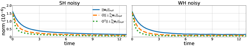
Figure 3: Exact convergence test with noisy data for both PDE systems, using only the null part of the norm (81). The WH system does not manifest a clear loss of convergence. Similar to Handmer and Szilagyi (2015) there is no evidence of exponential growth.

In Fig. 2 the rescaled norms for both smooth and noisy tests, for the artificial SH (80) and the full Bondi-Sachs system (78) and (79) that is WH are illustrated. The overlap of the rescaled norms indicates good second order convergence, whereas the lack of overlap suggests nonconvergence. For smooth given data both the SH and the WH systems exhibit good decent order convergence. However, for noisy given data only the SH has the appropriate convergence. This feature is expected, as noisy given data are important to demonstrate WH in numerical experiments Calabrese et al. (2006); Giannakopoulos et al. (2020). These results are compatible with earlier tests with random noise that demonstrated the lack of exponential growth in the solution Handmer and Szilagyi (2015). In Fig. 3 the sum only over the null hypersurface from (81) is shown, that is similar to earlier tests. The loss of convergence in the WH system is less severe than for the full norm (81), and there is no sign of exponential growth in the solution. This fact alone may be evidence for numerical stability in the colloquial sense that the code does not crash but, as we demonstrate in Fig. 2, is not enough evidence for convergence. It becomes apparent then that the choice of norm in which the convergence tests are performed is crucial. A norm that is compatible with the PDE system under consideration should be used.

VII Conclusions

Characteristic formulations of GR are used in a number of cases such as gravitational waveform modeling, critical collapse and applications to holography. These formulations are most commonly built upon Bondi-like gauges. In Giannakopoulos et al. (2020) the EFEs were shown to be only weakly hyperbolic in second order metric form in two popular Bondi-like gauges. Computational experiments were performed on toy models to examine the consequences of this fact, with the conclusion that numerical convergence in the simplest desired norms does not occur. Building on Giannakopoulos et al. (2020), in this paper we showed that this weak hyperbolicity is caused by the gauge condition $g^{uA}=0$ common to all Bondi-like gauges. Subsequently we performed numerical experiments performed in full GR, and found that the conclusions of Giannakopoulos et al. (2020) indeed carry over; ill-posedness of the continuum PDE (in the natural equivalent of $L^{2}$) for the characteristic problem serves as an obstruction to convergence of the numerics (in a discrete approximation to the same norm).

To show that weak hyperbolicity was a pure gauge effect we had to jump through a number of technical hoops. We mapped the characteristic free evolution system to an ADM setup so that the results of Khokhlov and Novikov (2002); Hilditch and Richter (2016) could easily be used. This allowed us to distinguish among the gauge, constraint, and physical degrees in the linear, constant coefficient approximation. Crucially it is known that weakly hyperbolic pure gauges give rise to weakly hyperbolic formulations. We were able to show the former in a number of cases. Specifically, we have studied three Bondi-like setups: the affine null, the Bondi-Sachs proper and the double null gauges. All three have the same degenerate structure rendering the pure gauge subsystem weakly hyperbolic. We have thus argued that when the EFE are written in a Bondi-like gauge with at most second derivatives of the metric and there are nontrivial dynamics in at least two spatial directions, then, due to the weak hyperbolicity of the pure gauge subsystem, the resulting PDE system is only WH.

The implication of weak hyperbolicity is that the CIVP and CIBVP of GR are ill-posed in the natural equivalent of $L^{2}$ on these geometric setups. Therefore we carried out convergence tests in a discretized version of such a norm. The specific form of the norm is inspired by the characteristic toy models of Giannakopoulos et al. (2020). We performed the tests on the Bondi-Sachs gauge system (78) and (79) implemented in the PITTNull thorn of the Einstein Toolkit, as well as on the artificial strongly hyperbolic system (80). The norm used is compatible with the strongly hyperbolic model in the characteristic domain. The tests are performed with smooth and with noisy given data. For smooth data both the strongly and weakly hyperbolic systems model exhibit good convergence. But with noisy data only the strongly hyperbolic model retains this behavior. These findings are compatible with previous results Calabrese et al. (2006); Cao and Hilditch (2012); Giannakopoulos et al. (2020), namely that noisy given data are essential to reveal weak hyperbolicity in numerical experiments. We have furthermore seen that even with noisy data one might overlook this behavior if tests are performed in a norm that is not suited to the particular problem.

Given all of the above, the obvious approach to circumvent weak hyperbolicity is to adopt a different gauge. For applications in CCM this may be necessary, since it is otherwise not at all clear how a well-posedness result for the composite PDE problem could be obtained. Yet, as discussed in the Introduction, concerning purely characteristic evolution, symmetric hyperbolic formulations of GR employing Bondi-like gauges are known Rácz (2014); Cabet et al. (2014); Hilditch et al. (2020); Ripley (2021). At first sight this seems to contradict the claim that any formulation of GR inherits the pure gauge principal symbol within its own. But these formulations all promote the curvature to be an evolved variable, so the results of Hilditch and Richter (2016) do not apply. As we have seen in Sec. IV, taking an outgoing null derivative of the affine null pure gauge subsystem, we obtain a strongly hyperbolic PDE. It is thus tempting to revisit the model of Hilditch and Richter (2016) to investigate the conjecture that formulations of GR with evolved curvature can be built that inherit specific derivatives of the pure gauge subsystem. A deeper understanding of the relation between the latter and the Bondi-like formulations analyzed in this paper could suggest norms in which they are actually well-posed. Obtaining such a proof would help validate error estimates for numerical solutions so relevant for applications in gravitational wave astronomy. Work in this direction is ongoing and will be reported on elsewhere.