Harmonic Retrieval with $L_{1}$-Tucker Tensor Decomposition

Abstract

Harmonic retrieval (HR) has a wide range of applications in the scenes where signals are modelled as a summation of sinusoids. Past works have developed a number of approaches to recover the original signals. Most of them rely on classical singular value decomposition, which are vulnerable to unexpected outliers. In this paper, we present new decomposition algorithms of third-order complex-valued tensors with $L_{1}$-principle component analysis ($L_{1}$-PCA) of complex data and apply them to a novel random access HR model in presence of outliers. We also develop a novel subcarrier recovery method for the proposed model. Simulations are designed to compare our proposed method with some existing tensor-based algorithms for HR. The results demonstrate the outlier-insensitivity of the proposed method.

1 Introduction

Harmonic retrieval (HR) is a vital problem in signal processing and has been applied to various areas, e.g., acoustic identification [1], digital communication [2] and biomedical processing [3]. The time-domain signals in HR model are naturally described as the summation of sinusoids. The goal of the HR problem is to retrieve the original subsignals from received noisy signals.

Researchers have proposed diverse methods to solve this problem. Kumaresan et al. [4] presented a technique based on linear prediction and singular value decomposition (SVD) to recover the pole-zero model in noises and then devised another nonlinear optimization method [5] to solve the same model. Papadopoulos et al. [6] came up with an estimation scheme based on high-order statistics. Kung et al. [7] presented a subspace approximation method based on SVD. Papy et al. [8] proposed a tensor Tucker-decomposition method, which is combined with the frequency recovery technique called ESPRIT [9] to solve HR problem. The tensor Tucker-decomposition method is a generalization of matrix principle component analysis (PCA) [10]. However, this technique cannot directly adapt to sporadic outliers due to the obvious outlier-sensitivity of Frobenius norm in the objective function in conventional Tucker-decomposition methods. To cope with outliers or non-Gaussian noises, some robust approaches [11, 12, 13] for HR are presented.

In this paper, to enhance robustness against outliers, we employ complex $L_{1}$-PCA [14, 15] in Tucker-decomposition method for HR. $L_{1}$-PCA robustify conventional PCA scheme against outliers and shows well outlier-resistance property in online outlier rejection [16] and streetscape Internet of Things [17].

The main contributions of this work are as follows: First, we develop two $L_{1}$-Tucker decomposition algorithms based on $L_{1}$-PCA to cope with the outliers in HR and convergence analyses are performed. Second, we present a novel subcarrier sorting method (SCSM) for the proposed random access HR model. Simulation results show that SCSM yields more accurate results than conventional ESPRIT method, and the proposed $L_{1}$-Tucker decomposition algorithms outperform some existing tensor-based algorithms in terms of outlier robustness.

The paper is organized as follows. In Section 2, we introduce the basic HR model and Tucker decomposition. In Section 3, we reformulate the HR problem (1) with a random access model, apply $L_{1}$-PCA into Tucker decomposition algorithms for solving the model and propose novel method for subcarrier recovery. In Section 4, some numerical experiments are presented for comparison between our proposed method and other tensor-based methods for HR. Finally, conclusions are drawn.

2 Preliminaries

2.1 Notations and Operators

For an integer $n$, denote $[n]=\{1,2,\ldots,n\}$. An $m$th-order tensor $\mathcal{A}\in\mathbb{C}^{I_{1}\times\cdots\times I_{m}}$ is an $m$-way array of complex numbers, which can be written as $\mathcal{A}=(\mathcal{A}_{i_{1}\cdots i_{m}}),i_{j}\in[I_{j}],j\in[m].$ Some tensor-related concepts in this paper are listed as follows:

• $k$-mode product $\times_{k}$: product between an $m$th-order tensor $\mathcal{A}\in\mathbb{C}^{I_{1}\times\cdots\times I_{m}}$ and a matrix $M_{k}\in\mathbb{C}^{R_{k}\times I_{k}}$, which is denoted as $(\mathcal{A}\times_{k}M_{k})_{i_{1}\ldots i_{k-1}ji_{k+1}\ldots i_{m}}=\sum_{i_{k}=1}^{I_{k}}a_{i_{1}\ldots i_{k-1}i_{k}i_{k+1}\ldots i_{m}}M_{ji_{k}}$ for $\forall i_{l}\in[I_{l}],\forall l\in[m]$ and $l\neq k,\forall j\in[R_{k}]$.

• $k$-mode fiber and $k$-mode unfolding: $k$-mode fiber is $I_{k}$-length vector $\mathcal{A}_{i_{1}\ldots i_{k-1}:i_{k+1}\ldots i_{m}}$. $k$-mode unfolding recorded as $\mathcal{A}_{(k)}$, which aligns all $k$-mode fibers of $\mathcal{A}$ as the columns of an $I_{k}\times\prod_{l\neq k}I_{l}$ matrix with the lexicographical order of $i_{1},\ldots,i_{k-1},i_{k+1},\ldots,i_{m}$. Then the $k$-mode product can be reformulated as $(\mathcal{A}\times_{k}M_{k})_{(k)}=M_{k}\mathcal{A}_{(k)}.$

• $n$-rank [10]: for each $n\in[m]$, $n$-rank of tensor $\mathcal{A}$ is denoted as $r_{n}=rank(col(\mathcal{A}_{(n)}))$. Moreover, $\mathcal{A}$ is called an $(r_{1},\cdots,r_{m})$-rank tensor.

• frontal-slice-Hankel (fs-Hankel) tensor: we call a tensor $\mathcal{H}\in\mathbb{C}^{I_{1}\times\cdots\times I_{m}}$ fs-Hankel tensor if for $i_{m}$-th ($i_{m}\in[I_{m}]$) frontal slice of tensor $\mathcal{H}$, there exists an $(I_{1}\!+\!\cdots\!+\!I_{m-1}\!-\!m\!+\!2)$-dimensional generating vector $\mathbf{h}^{(i_{m})}$ such that $\mathcal{H}_{i_{1}\ldots i_{m}}=\mathbf{h}^{(i_{m})}_{i_{1}+\ldots+i_{m-1}-m+2}.$

The complex sign operator of matrix $A\in\mathbb{C}^{m\times n}$ is $sgn(A)=(A_{ij}/|A_{ij}|)_{m\times n}.$ Assume SVD of $A\in\mathbb{C}^{m\times n}$ is formulated as $A=UDV^{H},$ where $D$ is diagonal and $U,V$ are column-unitary. Then the orthogonal projection operator $unt(A)$ is defined as $unt(A)=UV^{H}.$

2.2 The HR Model and Tucker Decomposition of Tensors

In HR problem, the receiver observes a series of discrete time-domain signals, which are formulated as

$$\textbf{x}_{n}=\sum_{k=1}^{K}\textbf{c}_{k}e^{j\omega_{k}t_{n}}+\textbf{q}_{n},\quad n=0,1,\ldots,N-1,$$ (1)

where $\textbf{x}_{n}$ is the $n$-th signal sample, $K$ is the number of subcarriers, $\omega_{k},\textbf{c}_{k}$ are $k$-th pulsation and corresponding complex amplitude $c_{k}$, respectively. $N$ is the number of samples, $\textbf{q}_{n}$ are noises, and $t_{n}=n\Delta t,$ where $\Delta t$ is the sampling time interval. We need to recover the pulsations $\omega_{k}$ and corresponding complex amplitude $\textbf{c}_{k}$ for all $k\in[K]$. Let $z_{k}=e^{j\omega_{k}\Delta t}$ be the $k$-th pole of the signal, then (1) is expressed as

$$\textbf{x}_{n}=\sum_{k=1}^{K}\textbf{c}_{k}z_{k}^{n}+\textbf{q}_{n},\quad n=0,1,\ldots,N-1.$$ (2)

Tucker decomposition is a powerful method to solve (2) since the signals can be naturally stacked in an Hankel tensor of which each unfold matrix has a Vandermonde form [8].

Define $\mathbb{U}^{m\times n}\!=\!\{X\!\in\!\mathbb{C}^{m\times n}|X^{H}X\!=\!I_{n}\}.$ The Tucker decomposition of $m$th-order tensor $\mathcal{X}$ is written as

$$\mathcal{X}\approx\mathcal{C}\times_{1}M_{1}\cdots\times_{m}M_{m},$$ (3)

where $\mathcal{X}\in\mathbb{C}^{I_{1}\times\ldots\times I_{m}},\mathcal{C}\in\mathbb{C}^{R_{1}\times\ldots\times R_{m}},$ and $M_{i}\in\mathbb{U}^{I_{i}\times R_{i}},\forall i\in[m].$ $\mathcal{C}$ is called the core tensor, and $i$-th factor matrix $M_{i}$ can be considered as the principal components of $i$-mode unfolding of $\mathcal{X}$. If $R_{i}=I_{i},\forall i\in[m],$ there exist $\mathcal{C}\in\mathbb{C}^{I_{1}\times\ldots\times I_{m}}$ and unitary matrices $M_{i}$ such that two sides of (3) are equal [18]. For generic tensor, when $R_{i}<I_{i},\forall i\in[m],$ it is usually infeasible for equality (3) to hold, but the smaller core tensor $\mathcal{C}$ can be deemed as a compression or a low-rank approximation of $\mathcal{X}$. Hence, the generalized Tucker decomposition is to find the best $(R_{1},\cdots,R_{m})$-rank approximation of $\mathcal{X}$, which can be modeled as

$$\mathop{\arg\min}_{\begin{subarray}{c}\mathcal{C}\in\mathbb{C}^{R_{1}\times\ldots\times R_{m}}\\ M_{i}\in\mathbb{U}^{I_{i}\times R_{i}},i\in[m]\end{subarray}}\lVert\mathcal{X}-\mathcal{C}\times_{1}M_{1}\cdots\times_{m}M_{m}\rVert_{F}=\mathop{\arg\max}_{\begin{subarray}{c}M_{i}\in\mathbb{U}^{I_{i}\times R_{i}},i\in[m]\\ \mathcal{C}=\mathcal{X}\times_{1}M_{1}^{H}\cdots\times_{m}M_{m}^{H}\end{subarray}}\lVert\mathcal{X}\times_{1}M_{1}\cdots\times_{m}M_{m}\rVert_{F}.$$ (4)

3 Harmonic Retrieval with $L_{1}$-Tucker Decomposition of Complex Tensors

3.1 System Model and Tensor-based Method with ESPRIT

Here we consider a random access multi-symbol HR model close to real communication scenario, which has an exponential structure similar to (1) but transmits signal on discrete frequencies. Assume there are $K\!-\!1$ available subcarriers with poles $z_{k}=e^{j2\pi k/K},k\in[K\!-\!1]$ and $K_{a}$ transmitters each randomly choose a different subcarrier to transmit symbols, respectively. The receiver observes the composite signals by sampling $Q$ continuous symbols. The time-domain samples are formulated as

$$\textbf{x}_{n}^{(q)}=\sum_{k=1}^{K-1}a_{k}\textbf{c}_{k}^{(q)}z_{k}^{n}+\textbf{q}_{n}^{(q)},\quad 0\leq n<N,q\in[Q],$$ (5)

where $\textbf{x}_{n}^{(q)}$ is the $n$-th composite sample of $q$-th symbol, $a_{k}=1($or $0)$ indicates that the $k$-th subcarrier is active (or inactive), $\textbf{c}_{k}^{(q)}$ is the $q$-th transmitted symbol on $k$-th subcarrier and is chosen from the given constellation, e.g., QPSK, $\textbf{q}_{n}^{(q)}$ is additive white Gaussian noise and the sampling interval is set as $\Delta t=1$. The receiver should recover the active subcarriers and corresponding transmitted symbols without knowing activity of transmitters and subcarriers. Like in [8], we assume that $K_{a}$ is known in advance.

The HR model (5) can be solved by the tensor-based method introduced in [8]. We sketch the main idea as follows. The samples can be stacked in a third-order fs-Hankel tensor $\bm{\mathcal{H}}\in\mathbb{C}^{I_{1}\times I_{2}\times Q}$ which satisfies $I_{1}+I_{2}-1=N,$ i.e.,

$$\bm{\mathcal{H}}_{i_{1}i_{2}q}=\textbf{x}_{i_{1}+i_{2}-2}^{(q)}=\sum_{k=1}^{K-1}a_{k}\textbf{c}_{k}^{(q)}(z_{k}^{i_{1}-1}z_{k}^{i_{2}-1})+\textbf{q}_{i_{1}+i_{2}-2}^{(q)},\forall q\in[Q],i_{j}\in[I_{j}],j=1,2.$$ (6)

Here $I_{1}$ and $I_{2}$ should be larger than $K_{a}$. Define the Vandermonde vector set as

$$W^{(j)}=\{w_{i}^{(j)}=\frac{1}{I_{j}}(1,z_{i},\ldots,z_{i}^{I_{j}-1})^{T}|i\in[K-1]\},\qquad W_{\text{active}}^{(j)}=\{w_{i}^{(j)}|a_{i}=1\},\qquad j=1,2.$$ (7)

In the noise-free case, the column subspace of $\bm{\mathcal{H}}_{(j)}$ is exactly spanned by $W_{\text{active}}^{(j)}$. The $(K_{a},K_{a},Q)$-rank Tucker decomposition of $\bm{\mathcal{H}}$,

$$\bm{\mathcal{H}}\approx\widetilde{\mathcal{C}}\times_{1}\widetilde{\textbf{U}}_{1}\times_{2}\widetilde{\textbf{U}}_{2}\times_{3}\widetilde{\textbf{Q}},$$ (8)

estimates the column subspace of $\bm{\mathcal{H}}_{(j)}$ with factor matrix $\widetilde{\textbf{U}}_{j}\in\mathbb{U}^{I_{j}\times K_{a}},j=1,2$. In terms of the immanent shift-invariance property of $span(W_{\text{active}}^{(j)})$, we solve the matrix equation

$$\widetilde{\textbf{U}}_{j}(2:I_{i},:)={\widetilde{\textbf{U}}}_{j}(1:I_{i}-1,:)\widetilde{\textbf{Z}}.$$ (9)

to obtain the solution $\widetilde{\textbf{Z}}^{*}$, then all eigenvalues $\hat{z}_{k},k\in[K_{a}]$ of $\widetilde{\textbf{Z}}^{*}$ are regarded as the estimations of poles of $K_{a}$ active subcarriers. By substituting the hard-decision of $\hat{z}_{k},k\in[K_{a}]$ into (5) and solving the linear system of $\textbf{c}_{k}^{(q)}$, we can obtain the estimations of symbols and the model (5) is completely recovered. The above subcarrier recovery scheme is called ESPRIT [9].

3.2 $L_{1}$-Tucker Decomposition of Third-Order Complex Tensor

The most important step of the subspace method introduced in the last subsection is to compute the approximate Tucker decomposition (8). Performance of a Tucker decomposition algorithms depends on its accuracy of separating initial signals (2) from noises. Higher-order singular value decomposition (HOSVD) [19] and higher-order orthogonal iteration (HOOI) [20] are two most popular algorithms for Tucker decomposition. Both two algorithms employ traditional PCA [21] in the iteration for each tensor mode to extract principal components of the tensor-unfolding matrices, which is deemed as signal extraction from noises.

For any given matrix $\textbf{X}\in\mathbb{C}^{D\times N},$ classical PCA method solves the optimization problem,

$$\textbf{P}_{{Frob-opt}}=\mathop{\arg\max}_{\textbf{P}\in\mathbb{U}^{D\times K}}\lVert\textbf{P}^{H}\textbf{X}\rVert_{F}$$ (10)

to obtain the first $K$ principal components of X, where $\lVert\textbf{A}\rVert_{F}=\sqrt{\sum_{i,j}|\textbf{A}_{i,j}|^{2}}$ is the Frobenius norm. However, due to the Frobenius-norm objective function, classical PCA is severely sensitive to heavy noises or outliers, which are inevitable in reality due to bursty interference in communication channels. Thus we consider a more robust method, $L_{1}$-PCA [14], to resolve this issue. The $L_{1}$-PCA replaces the Frobenius-norm in (10) with the $L_{1}$-norm operator $\lVert\textbf{A}\rVert_{1}=\sum_{i,j}|\textbf{A}_{ij}|$ and then gives as

$$\textbf{P}_{L_{1}-opt}=\mathop{\arg\max}_{\textbf{P}\in\mathbb{U}^{D\times K}}\lVert\textbf{P}^{H}\textbf{X}\rVert_{1}.$$ (11)

Algorithm 1 [14] reviews the convergent alternative iteration scheme for solving (11).

Algorithm 1 Algorithm for $L_{1}$-PCA$(\textbf{X},K,\textbf{P}^{(0)},\delta)$ [14]

0:  $\textbf{X}\in\mathbb{C}^{D\times N},K<$ rank$(\textbf{X}),\delta>0,k=1,$ initial matrix $\textbf{P}^{(0)}\in\mathbb{U}^{D\times K}$

0:  $\textbf{P}_{L_{1}-opt}$, the optimize solution of (11)

1:  $B^{(0)}=sgn(\textbf{X}^{H}\textbf{P}^{(0)})\in\mathbb{C}^{N\times K}$

2:  $B^{(k)}\leftarrow sgn(\textbf{X}^{H}unt(\textbf{X}B^{(k-1)}))$

3:  while $|\rVert\textbf{X}B^{(k)}\rVert_{*}-\rVert\textbf{X}B^{(k-1)}\rVert_{*}|>\delta$  do

4:     $B^{(k+1)}\leftarrow sgn(\textbf{X}^{H}unt(\textbf{X}B^{(k)}))$

5:     $k\leftarrow k+1$

6:  end while

7:  return  $\textbf{P}_{L_{1}-opt}\leftarrow unt(\textbf{X}B^{(k)})$

When the HR model (1) is interfered by outliers, we can replace the subspace estimation step in the existing Tucker-decomposition methods, HOSVD and HOOI, with $L_{1}$-PCA to enhance robustness. To be consistent with the new PCA scheme, the objective function (4) of approximate Tucker decomposition is adjusted in $L_{1}$-norm formula:

$$\mathop{max}_{\textbf{U}_{i}\in\mathbb{U}^{I_{i}\times K},i=1,2,3}\lVert\bm{\mathcal{H}}\times_{1}\textbf{U}_{1}\times_{2}\textbf{U}_{2}\times_{3}\textbf{U}_{3}\rVert_{1}.$$ (12)

Then we can naturally embed the Algorithm 1 into the subspace estimation step of HOSVD and obtain the Algorithm 2 named as $L_{1}$-Third Order Tucker Decomposition ($L_{1}$-TOTD). Algorithm 2 also converges since it only utilizes $L_{1}$-PCA once for each mode of the given tensors.

Algorithm 2 $L_{1}$-TOTD

0:  $\bm{\mathcal{H}}\in\mathbb{C}^{I_{1}\times I_{2}\times I_{3}},K>0,\delta>0,$ $\{\textbf{U}^{(0)}_{i}\in\mathbb{U}^{I_{i}\times K}\}$

0:  Factor matrices $\textbf{U}_{i}$ for each mode-$i$

1:  for $i=1,2,3$ do

2:     $\textbf{U}_{i}\leftarrow L_{1}$-PCA$(\bm{\mathcal{H}}_{(i)},K,\textbf{U}^{(0)}_{i},\delta)$

3:  end for

4:  return  $\{\textbf{U}_{i}\in\mathbb{C}^{I_{i}\times K}\}$

Another classical Tucker decomposition algorithm, HOOI, also relies on PCA during each sub-iteration for updating the factor matrices of each tensor mode. We also embed the $L_{1}$-PCA scheme into HOOI and gain the $L_{1}$-Third Order Orthogonal Iteration ($L_{1}$-TOOI) method as Algorithm 3. For instance, when the procedure runs to update the $1$-mode factor matrix, it can be formulated as an $L_{1}$-PCA problem,

$$\textbf{U}_{1}\leftarrow\mathop{\arg\max}_{\textbf{U}\in\mathbb{U}^{I_{1}\times K}}\lVert\bm{\mathcal{H}}_{(1)}\times_{1}\textbf{U}\times_{2}\textbf{U}_{2}\times_{3}\textbf{U}_{3}\rVert_{1}=\mathop{\arg\max}_{\textbf{U}\in\mathbb{U}^{I_{1}\times K}}\lVert\textbf{U}^{H}H_{1}\rVert_{1},$$ (13)

where $H_{1}=\bm{\mathcal{H}}_{(1)}(\textbf{U}_{3}\otimes\textbf{U}_{2})$ and $\otimes$ is the Kronecker product.

Algorithm 3 $L_{1}$-TOOI

0:  $\bm{\mathcal{H}}\in\mathbb{C}^{I_{1}\times I_{2}\times I_{3}},K>0,\delta>0$

0:  Factor matrices $\textbf{U}_{i}$ for each mode-$i$

1:  Compute initial factor matrices $\{\textbf{U}_{i}^{(0)}\in\mathbb{U}^{I_{i}\times K}\}$ by Algorithm 2, $p=0$

2:  while Not converging do

3:     $p\leftarrow p+1$

4:     for $i=1,2,3$ do

5:        $H_{i}^{(p)}\leftarrow\bm{\mathcal{H}}_{(i)}(\otimes_{j=3,\ldots,i+1}\textbf{U}_{j}^{(p-1)}\otimes_{j=i-1,\ldots,1}\textbf{U}_{j}^{(p)})$

6:        $\textbf{U}_{i}^{(p)}\leftarrow L_{1}$-PCA$(H_{i}^{(p)},K,\textbf{U}_{i}^{(p-1)},\delta)$

7:     end for

8:  end while

9:  return  $\{\textbf{U}_{i}^{(p)}\in\mathbb{C}^{I_{i}\times K}\}$

The convergence of Algorithm 3 is supported by the monotonicity of alternative iteration, which is illustrated in the following Theorem 3.1.

Theorem 3.1.

For any $p\geq 1$, the value in (12) monotonically increases within the $p$-th iteration (Line 3-7) of Algorithm 3 and between adjacent iterations, i.e.,

$$\lVert(\textbf{U}_{1}^{(p)})^{H}H_{1}^{(p)}\rVert_{1} \leq\lVert(\textbf{U}_{2}^{(p)})^{H}H_{2}^{(p)}\rVert_{1}\leq\lVert(\textbf{U}_{3}^{(p)})^{H}H_{3}^{(p)}\rVert_{1},$$ (14)

$$\lVert(\textbf{U}_{3}^{(p)})^{H}H_{3}^{(p)}\rVert_{1} \leq\lVert(\textbf{U}_{1}^{(p+1)})^{H}H_{1}^{(p+1)}\rVert_{1}.$$ (15)

Proof.

The first inequality in (14) is derived from the following inequalities,

$$\lVert(\textbf{U}_{1}^{(p)})^{H}H_{1}^{(p)}\rVert_{1}=\lVert(\textbf{U}_{2}^{(p-1)})^{H}H_{2}^{(p)}\rVert_{1}=\lVert(P_{2}^{(p,0)})^{H}H_{2}^{(p)}\rVert_{1}\leq\lVert(P_{2}^{(p,k)})^{H}H_{2}^{(p)}\rVert_{1}=\lVert(\textbf{U}_{2}^{(p)})^{H}H_{2}^{(p)}\rVert_{1},$$ (16)

where $P_{2}^{(p,0)}=\textbf{U}_{2}^{(p-1)}$ and $P_{2}^{(p,k)}=\textbf{U}_{2}^{(p)}$ are the input matrix and output result of $L_{1}$-PCA$(H_{2}^{(p)},K,\textbf{U}_{2}^{(p-1)})$, respectively. The inequality sign in (16) is supported by the monotonically increasing of Algorithm 1 [14]. The second inequality in (14) can be verified in a similar manner. Therefore, the monotonic increasing property holds in each iteration. On the other hand, between two adjacent iterations, we have

$$\lVert(\textbf{U}_{3}^{(p)})^{H}H_{3}^{(p)}\rVert_{1}=\lVert(\textbf{U}_{1}^{(p)})^{H}H_{1}^{(p+1)}\rVert_{1}=\lVert(P_{1}^{(p+1,0)})^{H}H_{1}^{(p+1)}\rVert_{1}\leq\lVert(P_{1}^{(p+1,k)})^{H}H_{1}^{(p+1)}\rVert_{1}=\lVert(\textbf{U}_{1}^{(p+1)})^{H}H_{1}^{(p+1)}\rVert_{1},$$

where $P_{1}^{(p+1,0)}=\textbf{U}_{1}^{(p)}$ and $P_{1}^{(p+1,k)}=\textbf{U}_{1}^{(p+1)}$ are the input matrix and output result of $L_{1}$-PCA$(H_{1}^{(p+1)},K,\textbf{U}_{1}^{(p)})$, respectively. Therefore, (15) holds for any $p\geq 1$. ∎

The monotonic increasing property, in conjunction with the fact that (12) is upper bounded since its domain is compact, implies the convergence of Algorithm 3. However, as (12) is not convex, we cannot make sure that the Algorithm 3 converges to the global optimal solution for any initialization $\textbf{U}_{i}^{(0)},i=1,2,3.$ Like the initialization strategy for HOOI [10, 22], we firstly perform $L_{1}$-TOTD and take the results as an initialization of $L_{1}$-TOOI, which helps the algorithm convergent to a better stationary point.

3.3 Subcarrier Sorting Method (SCSM) for Subcarrier Recovery

In presence of heavy noises and outliers, the factor matrices in the Tucker decomposition (8) have severe deviations, which leads to apparent perturbations in solving (9). We present a more robust subcarrier recovery method without solving (9) to address this issue. Before stating the proposed method, we first prove the following lemma.

Lemma 3.1.

Suppose $V=\{v_{i}\}_{i=1}^{m}\subset\mathbb{C}^{n}(n<m)$ is a set of unit-norm vectors satisfying that any $n$ vectors in V are linearly independent, and $\textbf{U}\in\mathbb{U}^{n\times k}.$ If there exists an index subset $I_{0}\subset[m]$ with $|I_{0}|=k$ such that the column space of U is spanned by $V_{0}=\{V_{i},i\in I_{0}\}$, then

$$\lVert v_{p}^{H}\textbf{U}\rVert_{F}^{2}<1=\lVert v_{i}^{H}\textbf{U}\rVert_{F}^{2},\quad\forall p\notin I_{0},\forall i\in I_{0}.$$ (17)

Proof.

Let $\textbf{U}=(\textbf{U}_{1},\ldots,\textbf{U}_{k}),$ then $\{\textbf{U}_{i}\}_{i=1}^{k}$ is a set of orthonormal bases of $span(V_{0})$ and we expand it into complete orthonormal bases of $\mathbb{C}^{n}$, which is denoted as $\{\textbf{U}_{i}\}_{i=1}^{n}.$ Therefore, for any $i\in[m],$ we decompose $v_{i}$ into $v_{i}=\sum_{s=1}^{n}(\textbf{U}_{s}^{H}v_{i})\textbf{U}_{s}.$ Then $\sum_{s=1}^{n}\lVert\textbf{U}_{s}^{H}v_{i}\rVert_{F}^{2}=\lVert v_{i}\rVert_{F}^{2}=1.$ Since $\forall i\in I_{0},\forall s>k,\textbf{U}_{s}^{H}v_{i}=0$, we have

$$\lVert v_{i}^{H}\textbf{U}\rVert_{F}^{2}=\sum_{s=1}^{k}\lVert\textbf{U}_{s}^{H}v_{i}\rVert_{F}^{2}=\sum_{s=1}^{n}\lVert\textbf{U}_{s}^{H}v_{i}\rVert_{F}^{2}=1.$$

For any $p\notin I_{0},$ $v_{p}\notin span(V_{0})$, there exists $q>k$ such that $\textbf{U}_{q}^{H}v_{p}\neq 0$, and

$$\lVert v_{p}^{H}\textbf{U}\rVert_{F}^{2}=\sum_{s=1}^{k}\lVert\textbf{U}_{s}^{H}v_{p}\rVert_{F}^{2}<\sum_{s=1}^{k}\lVert\textbf{U}_{s}^{H}v_{p}\rVert_{F}^{2}+\lVert\textbf{U}_{q}^{H}v_{p}\rVert_{F}^{2}\leq 1.\qed$$

In the noise-free case, the Vandermonde set $W^{(1)}$ in (7) and $\widetilde{\textbf{U}}_{i}=span(W_{\text{active}}^{(1)})\in\mathbb{C}^{I_{1}\times K_{a}}$ in (8) are in accordance with the conditions in Lemma 3.1. Hence, we can sort the elements of $S_{(1)}=\{\lVert w_{i}^{(1)H}\widetilde{\textbf{U}}_{1}\rVert_{F}\}_{i=1}^{K-1}$, and the largest $K_{a}$ elements correspond exactly to the $K_{a}$ active subcarriers. We call this method subcarrier sorting method (SCSM). The performance comparison between SCSM and ESPRIT in Fig. 1 illstrates robustness of SCSM in presence of outliers.

3.4 New Approach for Solving (5)

Based on the algorithms proposed in Section 3.2 and Section 3.3, we obtain a novel approach to deal with (5) as Algorithm 4.

Algorithm 4 Algorithm for solving (5)

0:  Signal samples $\{\textbf{x}_{n}^{(q)}\}_{n=0,q=1}^{N-1,Q}$ as (5), $I_{1},I_{2}$ that satisfies $I_{1}+I_{2}=N+1,K_{a}>0$

0:  Active subcarriers $z_{k}$ and corresponding symbols $\textbf{c}_{k}^{(q)}$ for $k\in[K_{a}],q\in[Q]$

1:  Construct an fs-Hankel tensor $\bm{\mathcal{H}}\in\mathbb{C}^{I_{1}\times I_{2}\times Q}$ with the signal samples ( 5)

2:  Obtain the factor matrices $\{\widetilde{\textbf{U}}_{i}\in\mathbb{C}^{I_{i}\times K}\}_{i=1,2}$ by $L_{1}$-TOTD or $L_{1}$-TOOI

3:  Run SCSM to search all $k_{a}$ active subcarriers $\hat{z}_{1},\ldots,\hat{z}_{K_{a}}$

4:  Substitute $\hat{z}_{1},\ldots,\hat{z}_{K_{a}}$ into the initial model (5) and solve the linear system to obtain symbol estimations $\hat{\textbf{c}}_{k}^{(q)},k\in[K_{a}],q\in[Q]$

The first step in Algorithm 4 is to choose a proper scale $I_{1}\times I_{2}\times Q$ for $\bm{\mathcal{H}}$. A necessary condition is that $I_{1},I_{2}>K$ since (9) requires that $\widetilde{\textbf{U}}_{i}^{\uparrow}$ is full-column-rank. Simulation results in [8, Fig. 6] advocated that slightly rectangular frontal slices may perform a little better than square slices. Nevertheless, the best scale of such rectangular slices is empirical and different in various scenes. For convenience, a common choice is to set $I_{1}=I_{2}$ as the scale of constructed fs-Hankel tensors, as a compromise between convenience and optimality.

3.5 Cramer-Rao Lower Bound (CRLB)

Here we present the Cramer-Rao lower bound (CRLB) for estimations of $\textbf{c}_{k}^{(q)}$ and $z_{k}$. Assume the power of AWGN in (5) is $\sigma^{2}$. Let $\textbf{x}=\{\textbf{x}_{n}^{(q)}\}_{n=0,q=1}^{N-1,Q}$, $\textbf{c}=\{\textbf{c}_{k}^{(q)}\}_{k=1,q=1}^{K},Q$ and $\textbf{z}=\{z_{k}\}_{k=1}^{K}$. The log-likelihood function is

$$\log p(\textbf{x}|\textbf{c},\textbf{z}) =\sum_{q=1}^{Q}\sum_{n=0}^{N-1}\log p(\textbf{x}_{n}^{(q)}|\textbf{c},\textbf{z})$$ (18)

$$=\sum_{q=1}^{Q}\sum_{n=0}^{N-1}\left(-\log\pi\sigma^{2}-\sigma^{-2}|\textbf{x}_{n}^{(q)}-\sum_{k=1}^{K}\textbf{c}_{k}^{(q)}z_{k}^{n\Delta t}|^{2}\right)$$

$$=-NQ\log\pi\sigma^{2}-\sigma^{-2}\sum_{q=1}^{Q}\sum_{n=0}^{N-1}|\textbf{x}_{n}^{(q)}-\sum_{k=1}^{K}\textbf{c}_{k}^{(q)}z_{k}^{n\Delta t}|^{2}.$$

According to [23, (13)], for any complex parameter $\theta$, we have

$$\text{CRLB}(\theta)=\frac{-1}{E\left[\frac{\partial^{2}\log p(x,\theta)}{\partial\theta^{*}\partial\theta}\right]}.$$ (19)

Then we have

$$\text{CRLB}(\textbf{c}_{k}^{(q)})=\frac{-1}{E\left[\frac{\partial^{2}\log p(\textbf{x}|\textbf{c},\textbf{z})}{\partial\textbf{c}_{k}^{(q)*}\partial\textbf{c}_{k}^{(q)}}\right]}=\frac{1}{E\left[\sigma^{-2}\sum\limits_{n=0}^{N-1}(z_{k}^{*})^{n\Delta t}z_{k}^{n\Delta t}\right]}=\sigma^{2}N^{-1},k=1,2,\cdots,K,$$ (20)

and

$$\text{CRLB}(z_{k})=\frac{-1}{E\left[\frac{\partial^{2}\log p(\textbf{x}|\textbf{c},\textbf{z})}{\partial z_{k}^{*}\partial z_{k}}\right]}=\frac{1}{E\left[\sigma^{-2}\sum\limits_{q=1}^{Q}\sum\limits_{n=0}^{N-1}(\Delta t)^{2}c_{k}^{(q)*}c_{k}^{(q)}\right]}=\frac{\sigma^{2}}{E(|c_{k}^{(q)}|^{2})\Delta t^{2}NQ}.$$ (21)

4 Numerical Experiments

In this section, we compare the performance of Algorithm 4 with conventional tensor Tucker-decomposition algorithms (HOOI, HOSVD) [8] and robust tensor decomposition method called IR-HOSVD [13].

In the following simulations, there are $K\!-\!1\!=\!49$ available subcarriers. With randomly selected different subcarriers, $K_{a}\!=\!6$ active transmitters simultaneously transmit $Q\!=\!12$ QPSK symbols in a frame, and the receiver samples $N\!=\!32$ time-domain samples for each symbol. We assume that the samples in (5) are sparsely interfered by outliers. The additive outliers are randomly and sparsely generated in signal samples and follow the Gaussian distribution with large variance $\sigma_{o}^{2}\!=\!20.$

The performance of an algorithm is evaluated in terms of the root mean square error (RMSE) of subcarriers and symbols, which are defined as

$$\text{RMSE}_{z}=\sqrt{\mathbb{E}\left(|\hat{z}_{k}-z_{k}|^{2}\right)},~{}\text{RMSE}_{c}=\sqrt{\mathbb{E}\left(|\hat{\textbf{c}}_{k}^{(q)}-\textbf{c}_{k}^{(q)}|^{2}\right)},$$ (22)

where $\hat{z}_{k},\hat{\textbf{c}}_{k}^{(q)}$ are estimations of $z_{k}$ and $\textbf{c}_{k}^{(q)}$, respectively.

First we test the robustness of SCSM by comparing it with ESPRIT, i.e., recovering subcarriers via solving equation (9). The comparison results under a series of signal-to-noise ratio (SNR) are illustrated in Figure 1. The results shows that SCSM consistently yields better results. Specifically, SCSM shows better outlier-separation ability than ESPRIT under low SNR.

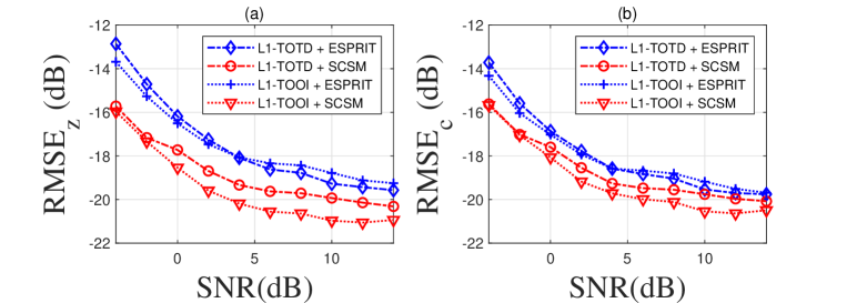
Figure 1: Robustness of two subcarrier recovery methods: SCSM and ESPRIT. $10\%$ of signal samples are interfered by outliers. (a) RMSE of subcarriers, (b) RMSE of symbols

Figure 2 reveals the comparison among different tensor-based methods for solving (5) in terms of RMSE. The Cramer-Rao lower bound (CRLB) of (5) is given in [24]. Our proposed two algorithms significantly enhance the robustness of HOSVD and HOOI as illustrated by the contrast of red and black curves in Fig. 2. Moreover, our method also outperforms IR-HOSVD, especially in high SNR.

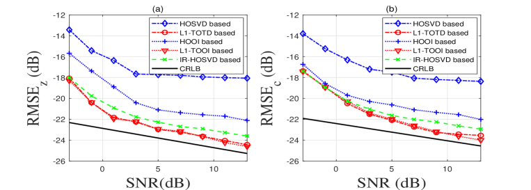
Figure 2: Comparison between Algorithm 4 and HOSVD/HOOI/IR-HOSVD in presence of outliers. $5\%$ of signal samples are interfered by outliers. (a) RMSE of subcarriers, (b) RMSE of symbols.

5 Conclusion

Through leveraging the weak outlier-sensitivity of $L_{1}$-norm, we introduce $L_{1}$-Tucker decomposition algorithm to solve the harmonic retrieval problem. We also develop an SCSM scheme for subcarrier detection. Simulation results show that our algorithm exhibits outlier-resistance property and outperforms existing tensor-based approaches for HR problem.

References

• [1] K. Kokkinakis, P. C. Loizou, Using blind source separation techniques to improve speech recognition in bilateral cochlear implant patients, Journal of the Acoustical Society of America 123 (4) (2008) 2379–2390. doi:10.1121/1.2839887.
• [2] S. Talwar, M. Viberg, A. Paulraj, Blind separation of synchronous co-channel digital signals using an antenna array. I. algorithms, IEEE Transactions on Signal Processing 44 (5) (1996) 1184–1197. doi:10.1109/78.502331.
• [3] V. Zarzoso, A. K. Nandi, Noninvasive fetal electrocardiogram extraction: Blind separation versus adaptive noise cancellation, IEEE Transactions on Biomedical Engineering 48 (1) (2001) 12–18. doi:10.1109/10.900244.
• [4] R. Kumaresan, D. Tufts, Estimating the parameters of exponentially damped sinusoids and pole-zero modeling in noise, IEEE Transactions on Acoustics Speech and Signal Processing 30 (6) (2003) 833–840. doi:10.1109/TASSP.1982.1163974.
• [5] R. Kumaresan, L. L. Scharf, A. K. Shaw, An algorithm for pole-zero modeling and spectral analysis, IEEE Transactions on Acoustics Speech and Signal Processing 34 (3) (1986) 637–640. doi:10.1109/TASSP.1986.1164843.
• [6] C. K. Papadopoulos, C. L. Nikias, Parameter estimation of exponentially damped sinusoids using higher order statistics, IEEE Transactions on Acoustics Speech and Signal Processing 38 (8) (1990) 1424–1436. doi:10.1109/29.57577.
• [7] S. Y. Kung, K. S. Arun, D. V. B. Rao, State-space and singular-value decomposition-based approximation methods for the harmonic retrieval problem, Journal of the Optical Society of America 73 (12) (1983) 1799–1811. doi:10.1364/JOSA.73.001799.
• [8] J. M. Papy, L. D. Lathauwer, S. V. Huffel, Exponential data fitting using multilinear algebra: The single-channel and multi-channel case, Numerical Linear Algebra with Applications 12 (8) (2010) 809–826. doi:10.1002/nla.453.
• [9] R. Roy, T. Kailath, ESPRIT - estimation of signal parameters via rotational invariance techniques, IEEE Transactions on Acoustics, Speech, and Signal Processing 37 (7) (1989) 984–995. doi:10.1109/29.32276.
• [10] T. G. Kolda, B. W. Bader, Tensor decompositions and applications, SIAM Review 51 (3) (2009) 455–500. doi:10.1137/07070111X.
• [11] S. Vorobyov, Y. Rong, N. Sidiropoulos, A. Gershman, Robust iterative fitting of multilinear models, IEEE Transactions on Signal Processing 53 (8) (2005) 2678–2689. doi:10.1109/TSP.2005.850343.
• [12] C. Qian, Y. Shi, L. Huang, H. C. So, Robust harmonic retrieval via block successive upper-bound minimization, IEEE Transactions on Signal Processing 66 (23) (2018) 6310–6324. doi:10.1109/TSP.2018.2875394.
• [13] F. Wen, H. C. So, Robust multi-dimensional harmonic retrieval using iteratively reweighted HOSVD, IEEE Signal Processing Letters 22 (12) (2015) 2464–2468. doi:10.1109/LSP.2015.2493521.
• [14] N. Tsagkarakis, P. P. Markopoulos, D. A. Pados, L1-norm principal-component analysis of complex data, IEEE Transactions on Signal Processing 66 (12) (2018) 3256–3267. doi:10.1109/TSP.2018.2821641.
• [15] D. G. Chachlakis, A. Prater-Bennette, P. P. Markopoulos, L1-norm tucker tensor decomposition, IEEE Access 7 (2019) 178454–178465. doi:10.1109/ACCESS.2019.2955134.
• [16] P. P. Markopoulos, M. Dhanaraj, A. Savakis, Adaptive L1-norm principal-component analysis with online outlier rejection, IEEE Journal of Selected Topics in Signal Processing 12 (6) (2018) 1131–1143. doi:10.1109/JSTSP.2018.2874165.
• [17] G. Sklivanitis, K. Tountas, N. Tsagkarakis, D. A. Pados, S. N. Batalama, Optimal joint channel estimation and data detection by L1-norm PCA for streetscape IoT, in: ICASSP 2020 - 2020 IEEE International Conference on Acoustics, Speech and Signal Processing (ICASSP), 2020, pp. 9051–9054. doi:10.1109/ICASSP40776.2020.9054507.
• [18] L. D. Lathauwert, B. D. Moort, J. Vandewallet, A multilinear singular value decomposition, SIAM Journal on Matrix Analysis and Applications 21 (4) (2000) 1253–1278. doi:10.1137/S0895479896305696.
• [19] L. Tucker, Some mathematical notes on three-mode factor analysis, Psychometrika 31 (3) (1966) 279–311. doi:10.1007/BF02289464.
• [20] L. D. Lathauwert, B. D. Moort, J. Vandewallet, On the best rank-1 and rank-$(r_{1},r_{2},\ldots,r_{n})$ approximation of higher-order tensors, SIAM Journal on Matrix Analysis and Applications 21 (4) (2000) 1324–1342. doi:10.1137/S0895479898346995.
• [21] H. Hotelling, Analysis of a complex of statistical variables into principal components., Journal of Educational Psychology 24 (1933) 498–520. doi:10.1037/h0071325.
• [22] C. A. Andersson, R. Bro, Improving the speed of multi-way algorithms: Part I. Tucker3, Chemometrics and Intelligent Laboratory Systems 42 (1) (1998) 93–103. doi:https://doi.org/10.1016/S0169-7439(98)00010-0.
• [23] A. van den Bos, A cramer-rao lower bound for complex parameters, IEEE Transactions on Signal Processing 42 (10) (1994) 2859–. doi:10.1109/78.324755.
• [24] Z. Luan, Z. Ming, Y. Wu, W. Han, X. Chen, B. Bai, L. Zhang, Harmonic retrieval with L1-Tucker tensor decomposition (2021). arXiv:2111.14780.