Interface-Induced Conservation of Momentum Leads to Chiral-Induced Spin Selectivity

Abstract

We study the non-equilibrium dynamics of electron transmission from a straight waveguide to a helix with spin–orbit coupling. Transmission is found to be spin-selective and can lead to large spin polarizations of the itinerant electrons. The degree of spin selectivity depends on the width of the interface region, and no polarization is found for single-point couplings. We show that this is due to momentum conservation conditions arising from extended interfaces. We therefore identify interface structure and conservation of momentum as crucial ingredients for chiral-induced spin selectivity, and confirm that this mechanism is robust against static disorder.

Chiral-induced spin selectivity (CISS) [1, 2] is an intriguing phenomenon wherein the chirality of organic molecules such as DNA [3], oligopeptides [4], bacteriorhodopsine [5] or photosystem I [6] induces notable spin dependence on various electronic processes. Experiments have demonstrated that unpolarized photoelectrons can become highly spin-polarized when transmitted through (mono-)layers of helical molecules, with the molecule’s handedness deciding the sign of the polarization [7, 8]. The CISS effect has also been observed for bound electron transport in the form of spin-dependent currents when helical molecules are placed between a substrate and an atomic force microscope (AFM) tip [9]. Naturally, such phenomena have attracted much interest in the field of spintronics that uses the electron spin to process information in nanodevices [10, 11, 12, 13, 14, 15]. More recently, the relations between electron spin, enantioselectivity and chemical reactivity in chiral molecules has also been the subject of increased attention [16, 17, 18, 19, 20]. Though it is apparent that the experimentally observed spin polarization is related to the spin–orbit coupling (SOC) experienced by the electrons moving through the helical or chiral structures, a consensus on the microscopic mechanism has not yet been reached [21].

In this work, we present a simple and natural model exhibiting CISS whose underlying mechanism can be rigorously understood using intuitive physical concepts: Electrons initially traveling along a SOC-free straight waveguide approach a helical waveguide (Fig. 1(a)) with SOC to which they can tunnel, resulting in an effective coupling region of width $\xi$ (Fig. 1(b)). We show that an initially spin-unpolarized electron wavepacket naturally becomes polarized after coming into proximity with the helix if the interaction region is not a single point, i.e., if $\xi>0$. This process can be repeated if the electron then comes into contact with further helices, amplifying the effect. We demonstrate that high spin polarization $\sim$50\text{\,}\mathrm{\char 37\relax}$$ can be achieved for moderate SOC strengths $\hbar\alpha\sim$1\text{\,}\mathrm{meV}\text{\,}\mathrm{nm}$$, despite the helical waveguide being modeled as a single one-dimensional channel without – contrary to previous theoretical studies – intramolecular

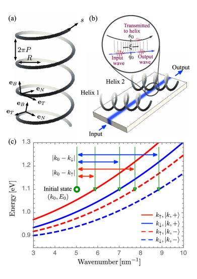
Figure 1: (a) Helix-shaped waveguide with radius $R$ and pitch $2\pi P$. At each point, a coordinate system is defined by the normal ($\mathbf{e}_{N}$), bi-normal ($\mathbf{e}_{B}$) and tangential ($\mathbf{e}_{T}$) vectors. (b) Schematic representation of multiple scattering events of a electron wavepacket traveling along a SOC-free waveguide. The scattering occurs over a region of non-zero length $\xi$, leading to a transmitted wavepacket in the helical waveguide and a remaining wavepacket in the free waveguide. (c) Spin-dependent dispersion relations of a helical waveguide. The initial wavenumber $k_{0}$ and energy $E_{0}$ of an input state are marked by a green circle. The difference between the input wavenumber $k_{0}$ and spin-dependent wavenumbers $k_{\uparrow}$ and $k_{\downarrow}$ of the $E_{0}$-energetically resonant eigenstates of the helical waveguide are highlighted by red and blue arrows, respectively.

multi-channel structures. However, when the SOC-free and helical waveguides are coupled only at a single point ($\xi\to 0$), the outgoing state remains unpolarized. As we will show in this work, these results can be rationalized in terms of spin-dependent inter-waveguide transmission probabilities, as an extended interaction region $\xi>0$ prescribes (partial) conservation of momentum, resulting in spin-selective transmissions due to spin–orbit coupling within the helix. Therefore, our work highlights the importance of interface modeling in CISS.

As shown in Fig. 1(a), each helical molecule is characterized by its radius $R$ and pitch $2\pi P$; we use the geometrical parameters of DNA, $R=$0.7\text{\,}\mathrm{nm}$$ and $2\pi P=$3.4\text{\,}\mathrm{nm}$$ [22], throughout. As a model for an electron traveling through the potential energy landscape of a helical molecule, we assume that an electron wavepacket propagates solely in the tangential direction $\mathbf{e}_{T}$ of a helical path due to a trapping potential acting in the normal $\mathbf{e}_{N}$ and binormal $\mathbf{e}_{B}$ directions. The electron’s dynamics can then be described by an effective one-dimensional quantum state in the form $\psi_{\uparrow}(s,t)\ket{\uparrow}+\psi_{\downarrow}(s,t)\ket{\downarrow}$, where $\ket{\uparrow}$ and $\ket{\downarrow}$ are the eigenstates of the Pauli matrix $\sigma_{z}$, $t$ is the time coordinate and $s$ represents the position on the helical path, as shown in Fig. 1(a). As in previous CISS models [23, 24, 25, 26, 27, 28], we assume that the electric field induced by the molecule is helical-symmetric and that the field on the helical path is oriented in the normal direction, $\mathbf{E}=E\mathbf{e}_{N}(s)$ with constant $E$, where the normal unit vector $\mathbf{e}_{N}(s)$ depends on the position $s$. The dynamics of the electron wavepacket is governed by an effective Hamiltonian [29] of the form

$$H_{h}=\frac{{p_{s}}^{2}}{2m_{h}}+U_{h}+\frac{\alpha}{2}\anticommutator{\bm{\sigma}\cdot\mathbf{e}_{B}(s)}{p_{s}},$$ (1)

where $p_{s}=-i\hbar\partial_{s}$ is the momentum operator in the tangential direction $\mathbf{e}_{T}(s)$, $m_{h}=10\,m_{e}$ is the effective electron mass [30, 31] with $m_{e}$ its rest mass, and $U_{h}$ is a constant potential energy shift. The last term in Eq. 1 represents the spin–orbit interaction, which is generally described by ${H_{\text{SOC}}}=-\bm{\sigma}\cdot(\bm{\alpha}\times\mathbf{p})$, where $\bm{\alpha}$ is proportional to $\mathbf{E}$ and quantifies the SOC strength via its magnitude $\alpha$. Thus, since we assume $\mathbf{E}$ parallel to $\mathbf{e}_{N}(s)$, we have $\bm{\alpha}=\alpha\mathbf{e}_{N}(s)$ and ${H_{\text{SOC}}}$ as shown in Eq. 1.

As shown in the SI, the eigenstates as a function of the helical position coordinate $s$ can be expressed as

$$\innerproduct{s}{k,\pm}=\frac{A_{\pm}e^{ik_{\uparrow}s}\ket{\uparrow}+e^{ik_{\downarrow}s}\ket{\downarrow}}{\sqrt{2\pi\left(1+\absolutevalue{A_{\pm}}^{2}\right)}},$$ (2)

with $D=\sqrt{R^{2}+P^{2}}$, where the spin-dependent wavenumbers are given by $k_{\uparrow}=k-(2D)^{-1}$ and $k_{\downarrow}=k+(2D)^{-1}$, and $A_{+}$ and $A_{-}$ are $k$-independent coefficients. This shows that there are two distinct groups of eigenstates, $\{\ket{k,+}\}$ and $\{\ket{k,-}\}$, with different energies and opposite spin polarizations $P_{\pm}=\expectationvalue{\sigma_{z}}=(\absolutevalue{A_{\pm}}^{2}-1)/(\absolutevalue{A_{\pm}}^{2}+1)$ which fulfill $P_{+}=-P_{-}$. In Fig. 1(c), the dispersion relation between energy $E(k,+)$ and wavenumber $k_{\uparrow}$ (or $k_{\downarrow}$) of the eigenstates $\{\ket{k,+}\}$ is shown in a red (or blue) solid line, where $U_{h}=$0.9\text{\,}\mathrm{eV}$$ and $\hbar\alpha=$10\text{\,}\mathrm{meV}\text{\,}\mathrm{nm}$$ are considered as an example. These $k_{\uparrow}$ and $k_{\downarrow}$ curves differ due to the correlations between spin states and wavenumbers induced by spin–orbit interaction, as shown in Eq. 2. Similarly, the two components of the dispersion relation of the $\{\ket{k,-}\}$ eigenstates are shown in red and blue dashed lines, respectively, in Fig. 1(c). These results demonstrate that when an electron with well-defined energy $E_{0}$ and wavenumber $k_{0}$ enters a helical waveguide in such a way that the energy of an electron wavepacket is conserved (such that $E_{0}=E(k,\pm)$), the wavenumber $k_{\uparrow}$ or $k_{\downarrow}$ of the helical eigenstate $\ket{k,\pm}$ will generally differ from $k_{0}$ of the input state. Importantly, the difference between wavenumbers can be smaller or larger depending on the incoming state’s polarization. In the case shown in Fig. 1(c), the difference is smaller for a spin-up state than for a spin-down state, $\absolutevalue{k_{0}-k_{\uparrow}}<\absolutevalue{k_{0}-k_{\downarrow}}$, as highlighted by red and blue arrows. Therefore, if the transition probability favors smaller differences between wavenumbers – that is, if momentum conservation is (at least partially) enforced – then a ${\ket{\uparrow}}$ state will transition to the helix more readily than a ${\ket{\downarrow}}$ state. As we will show shortly, this partial momentum conservation does indeed arise when the interfacial coupling is extended over a region rather than being point-like, thus constituting the centerpiece of our model. Finally, it follows from these preliminaries that an initially unpolarized mixed state will lose ${\ket{\uparrow}}$ population to the helix more quickly than ${\ket{\downarrow}}$: This results in a net negative spin polarization of the remaining electronic density that has not been transmitted to the helix, an effect which can be further amplified by repeated interactions with other helices.

To quantitatively model the relation between interfacial structure and momentum-conservation assisted spin filtering, we introduce a second one-dimensional waveguide. This second waveguide shall be governed by a free-space Hamiltonian in the form $H_{f}=(2m_{e})^{-1}{p_{q}}^{2}$, where $p_{q}=-i\hbar\partial_{q}$ is the momentum operator along a separate coordinate $q$, as shown in the inset of Fig. 1(b). The eigenstates of $H_{f}$ are spin-independent and given by $\innerproduct{q}{k}=(2\pi)^{-1/2}e^{ikq}$ with wavenumbers $k$ (and $\innerproduct{s}{k}=0$). We call this the free waveguide or free-space channel, as opposed to the helical waveguide. To model an inter-waveguide scattering process occurring over an extended region, we consider coupling between free (coordinate $q$) and helical waveguides ($s$) of the form

$$V(s,q)=V_{0}\exp(-\frac{(s-s_{0})^{2}}{2\xi^{2}})\delta\mathopen{}\mathclose{{}\left((s-s_{0})-(q-q_{0})}\right)$$ (3)

where $s$ and $q$ denote the position on the helical and free waveguide, respectively and $\delta(x)$ is the Dirac delta, which signifies that each position is coupled to exactly one position on the opposite waveguide. This $V(s,q)$ implies that when an electron wavepacket propagates in the free waveguide, the phase information of the input state, encoded as a function of the free-space coordinate $q$, is transferred to the helical waveguide over an extended width $\xi$ of the interface centered at $(s,q)=(s_{0},q_{0})$, as shown schematically in the inset to Fig. 1(b). When the input state of the free-space channel is a $\ket{\uparrow}$ state with wavenumber $k_{0}$, the coupling to a helical eigenstate $\ket{k,\pm}$ is given by

$$\absolutevalue{\!\matrixelement{k,{\pm}}{V}{k_{0},\uparrow}}^{2}=\left(\frac{{V_{0}}^{2}\xi^{2}}{2\pi}\frac{\absolutevalue{A_{\pm}}^{2}}{1+\absolutevalue{A_{\pm}}^{2}}\right)e^{-\xi^{2}\left(\Delta k\right)^{2}}$$ (4)

with $\Delta k=k_{\uparrow}-k_{0}$. We see that the coupling strength is stronger if the eigenstate $\ket{k,\pm}$ has a larger $\ket{\uparrow}$ component amplitude $\absolutevalue{A_{\pm}}$ (cf. Eq. 2). However, more importantly, as the width $\xi$ of the interface increases, the effective coupling strength becomes more sensitive to the momentum mismatch $\hbar\Delta k$, and as a result transfer occurs only if the wavenumber is conserved, $k_{\uparrow}\approx k_{0}$. On the other hand, when the interface is very narrow, $\xi\to 0$, the effective coupling strength becomes independent of $\Delta k$. In this case, the only information provided to a helical channel is the time-dependent amplitude of the input state at a single-point contact with the free waveguide. This makes scattering probabilities independent of changes in momentum, similar to the textbook problem of one-dimensional scattering at a step potential [32].

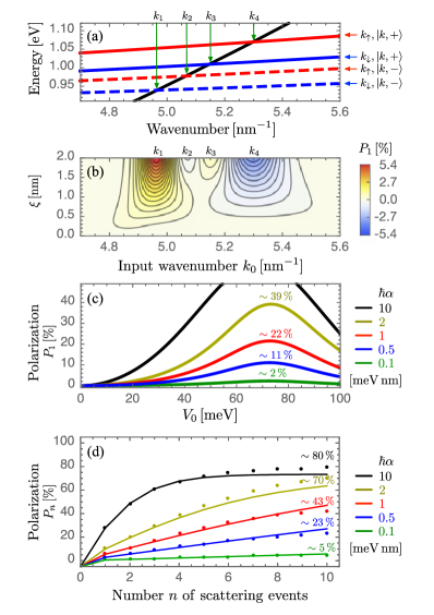
Figure 2: (a) Spin-dependent dispersion relations of a helical molecule (red and blue, cf. Fig. 1(c)), and the free-space dispersion relation (black), for $U_{h}=$0.9\text{\,}\mathrm{eV}$$ and $\hbar\alpha=$10\text{\,}\mathrm{meV}\text{\,}\mathrm{nm}$$. The $k_{1,2,3,4}$ of the four crossing points are highlighted by green arrows. (b) Spin polarization $P_{1}$ after a single scattering event as a function of input wavenumber $k_{0}$ and the interaction region width $\xi$ (cf. Fig. 1(b)). $U_{h}$ and $\alpha$ as in (a), with $V_{0}=$10\text{\,}\mathrm{meV}$$. (c) $P_{1}$ as a function of the interfacial coupling strength $V_{0}$ for $\xi=$1\text{\,}\mathrm{nm}$$. We use $k_{0}=$5.075\text{\,}{\mathrm{nm}}^{-1}$$ except for $\hbar\alpha=$10\text{\,}\mathrm{meV}\text{\,}\mathrm{nm}$$, where $4.975\text{\,}{\mathrm{nm}}^{-1}$ is considered due to the $\alpha$-dependence of the crossing points. (d) Spin polarization $P_{n}$ after $n$ scattering events with parameters as given in (c) and $V_{0}=$40\text{\,}\mathrm{meV}$$. Dots are numerical calculations, solid lines are transfer-matrix-based extrapolations.

To demonstrate that a non-zero length $\xi$ of the interface can induce the momentum-conservation assisted spin filtering, we consider a Gaussian initial electron state in the form

$$\innerproduct{q}{\psi_{i}^{\sigma}(t=0)}=\frac{1}{\pi^{\frac{1}{4}}\zeta^{\frac{1}{2}}}\exp(-\frac{(q-q_{i})^{2}}{2\zeta^{2}}+ik_{0}q)\ket{\sigma},$$ (5)

with $\sigma\in\{\uparrow,\downarrow\}$, and with an initial center position $q_{i}$ such that the amplitude at the interface around $q_{0}$ is negligible. This is a superposition of the eigenstates $\ket{k}$ of the free-space Hamiltonian $H_{f}$ such that $\absolutevalue{\innerproduct{k}{\psi_{i}^{\sigma}}}^{2}\propto e^{-(k-k_{0})^{2}\zeta^{2}}$, which is centered at $\expectationvalue{k}=\expectationvalue{p}/\hbar=k_{0}$ with an uncertainty $\sigma_{k}=\left(\sqrt{2}\zeta\right)^{-1}$ (we use $\zeta=100/k_{0}$ throughout). We can then apply time-dependent perturbation theory to first order in $V$ (Eq. 3), similar to Fermi’s Golden Rule, to obtain the probability that an incoming Gaussian state $\ket{\psi_{i}^{\sigma}}$ of polarization $\sigma$, Eq. 5, has transitioned to a helix eigenstate $\ket{k_{\text{out}},\pm}$, Eq. 2, in the long-time limit $t\to\infty$ (see SI for further details):

$$\lim_{t\to\infty}\absolutevalue{\innerproduct{k_{\text{out}},\pm}{\psi_{i}^{\sigma}(t)}}^{2}\\ \propto\absolutevalue{\int_{\mathbb{R}}e^{-\frac{\xi^{2}\left(\Delta k\right)^{2}}{2}-\frac{\zeta^{2}\left(k-k_{0}\right)^{2}}{2}-i\phi(k)}\,\delta\mathopen{}\mathclose{{}\left(\omega(k)}\right)\differential{k}}^{2},$$ (6)

where $\Delta k=k_{\sigma}-k$ and $\omega(k)=\hbar k^{2}/(2m_{e})-E(k_{\text{out}},\pm)/\hbar$, and $\phi(k)=(q_{i}-q_{0})k$ is a (largely irrelevant) phase. We see that in the long-time limit, energy is rigorously conserved during transitions, but momentum is only loosely conserved according to a Gaussian law, as predicted by Eq. 4. For small $\xi$ and/or $V_{0}$, such that the influence of $V(s,q)$ remains perturbative, this simple equation can be used to accurately describe the transition probabilities and therefore the spin polarizations of our model. We quantify the spin polarization arising from an initially unpolarized mixed state $\rho_{0}=\frac{1}{2}\left[\outerproduct{\psi_{i}^{\uparrow}}{\psi_{i}^{\uparrow}}+\outerproduct{\psi_{i}^{\downarrow}}{\psi_{i}^{\downarrow}}\right]$ with $\ket{\psi_{i}^{\sigma}}$ from Eq. 5 as

$$P_{1}=\Tr{\left[\mathcal{P}_{f}\rho_{1}\mathcal{P}_{f}^{\dagger}\right]\sigma_{z}}/\Tr{\mathcal{P}_{f}\rho_{1}\mathcal{P}_{f}^{\dagger}}$$

where $\rho_{1}$ is the state $\rho_{0}$ after passing through an interaction region with a helix, and $\mathcal{P}_{f}$ is the projector onto the free-waveguide component. The polarization $P_{n}$ after $n$ repeated interactions with separate helices is defined analogously using the state $\rho_{n}$, which is the result of scattering the state $\mathcal{P}_{f}\rho_{n-1}\mathcal{P}_{f}^{\dagger}$.

To expand our analysis to the non-perturbative regime, we calculate numerically the dynamics of the wavepacket using a standard finite-difference scheme (see SI), which further shows good agreement with Eq. 6 within the perturbative regime. We illustrate the rich physics of our model by demonstrating the effect of varying the interfacial length $\xi$ and the incoming momentum $\hbar k_{0}$: In Fig. 2(a), the dispersion relations of the spin components of the helical eigenstates $\ket{k,\pm}$ are shown in red and blue, in addition to that of the free-space eigenstates, shown in black. The dispersion curves are crossed at four different wavenumbers $k_{1,2,3,4}$, highlighted by green arrows. In Fig. 2(b), where $\hbar\alpha=$10\text{\,}\mathrm{meV}\text{\,}\mathrm{nm}$$ and $V_{0}=$10\text{\,}\mathrm{meV}$$, the spin polarization $P_{1}$ after a single scattering event is shown as a function of the input wavenumber $k_{0}$ and the width $\xi$ of the Gaussian coupling spectrum of the interface. As expected from the above discussion, the spin polarization is zero for $\xi=0$ (single-point coupling) and the spin polarization effect is enhanced as $\xi$ increases. At the crossing point of the momenta $k_{1,3}$ ($k_{2,4}$), the spin polarization becomes maximally positive (negative), as these momenta correspond to the ${\ket{\downarrow}}$ (${\ket{\uparrow}}$) component of the helical eigenstates, causing an incoming ${\ket{\downarrow}}$ (${\ket{\uparrow}}$) state to be transmitted to the helix with higher probability, as predicted by Eq. 6. In Fig. 2(c), where $\xi=$1\text{\,}\mathrm{nm}$$ and $k_{0}\approx$5\text{\,}{\mathrm{nm}}^{-1}$$, the spin polarization is displayed as a function of the interfacial coupling strength $V_{0}$ for different spin–orbit coupling strengths from $0.1\text{\,}\mathrm{meV}\text{\,}\mathrm{nm}10\text{\,}\mathrm{meV}\text{\,}\mathrm{nm}$. It is notable that even for weak spin–orbit coupling $\hbar\alpha=$0.1\text{\,}\mathrm{meV}\text{\,}\mathrm{nm}$$ and $1\text{\,}\mathrm{meV}\text{\,}\mathrm{nm}$, the spin polarization reaches values up to $\sim$2\text{\,}\mathrm{\char 37\relax}$$ and $\sim$22\text{\,}\mathrm{\char 37\relax}$$, respectively. Figure 2(d) shows the results of numerical simulations (shown as dots) with $V_{0}=$40\text{\,}\mathrm{meV}$$ demonstrating that the spin polarization is further enhanced when the input wavepacket is scattered multiple times by independent helices (cf. Fig. 1(b)). For example, in the case of weak spin–orbit coupling strength $\hbar\alpha=$1\text{\,}\mathrm{meV}\text{\,}\mathrm{nm}$$, the spin polarization is increased from $P_{1}\approx$6\text{\,}\mathrm{\char 37\relax}$$ to $P_{10}\approx$43\text{\,}\mathrm{\char 37\relax}$$ after 10 consecutive scattering events. Furthermore, using a transfer-matrix-like method, we can estimate the $n$-scattering polarization $P_{n}$ based only on the single-scattering data, which also shows that $\absolutevalue{P_{\infty}}<$100\text{\,}\mathrm{\char 37\relax}$$ is caused by spin-flip back-transfer from the helical to straight waveguide (solid lines in Fig. 2(d), see SI for details). These results demonstrate that high spin polarization can be obtained from initially unpolarized electrons when scattering occurs over an extended region of a helical molecule even for weak intrinsic SOC strength ($\hbar\alpha\lesssim$1\text{\,}\mathrm{meV}\text{\,}\mathrm{nm}$$).

Notice that the vanishing spin polarization in the case of single-point couplings is in line with the well-known fact that in one-dimensional theories, spin–orbit coupling can be removed by a unitary transformation and hence – on its own – cannot account for spin-filtering [33]. Previous studies have therefore claimed that multiple channels such as additional helix strands [34, 35] or orbitals [25, 36] are required to observe spin polarization. As shown in the SI, the extended nature of the interface coupling prevents spin-dependence in our model from being removed by a unitary transformation and no intramolecular multi-channel structure need be employed.

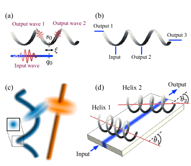
Figure 3: (a) Three-terminal setup where the tip of an electrode is coupled to a single helix over an extended region. An unpolarized input wavepacket is transmitted to the helix and results in oppositely polarized wavepackets traveling in opposite directions. (b) In a general $N$-terminal setup where all interfaces are point contacts, no spin polarization can be observed. (c) To incorporate geometrical effects, an inter-waveguide coupling matrix is calculated from the overlap between Gaussian cross-section slices: One slice–wedge pair is shown exploded. (d) Schematic representation of multiple scattering events with varying orientations of the helix axes. Helix 2 is shown in the locally parallel configuration $\theta_{2}\approx$52\text{\,}\mathrm{\SIUnitSymbolDegree}$$, whereas helix 1 is not.

The mechanism of momentum conservation and spin-dependent transmission can also be used to understand spin-polarized transport through a helical waveguide attached to leads: Figure 3(a) illustrates a three-terminal setup with an electrode tip coupled to a helix over a length $\xi$. A wavepacket transmitted to the helix splits into oppositely polarized wavepackets propagating in opposite directions inside the helix. In this case – as well as in any general $N$-terminal setup as depicted in Fig. 3(b) – average spin polarization vanishes if all couplings are point contacts.

Lastly, the coupling function $V(s,q)$ of Eq. 3 may be a simplification of the inter-waveguide coupling, as it does not directly depend on the 3D arrangement of the system. Therefore, to further validate our interface-based mechanism and test its robustness against disorder, we have calculated dynamics using a more elaborate coupling function $V(s,q)$ based on the 3D overlap between Gaussian cross-section wavefunctions occupying the straight and helical systems, as illustrated in Fig. 3(c). This more advanced coupling model naturally depends on the angle and distance between the helix and the straight waveguide, and it is also no longer diagonal in the sense that $V=0$ does not necessarily hold for $s-s_{0}\neq q-q_{0}$. Using this geometry-dependent model, we examine the influence of variations of the angle to the helix, illustrated in Fig. 3(d). The simpler coupling model of Eq. 3 is closest to the geometrical configuration in which the tangent vectors of the two waveguides are parallel at their point of least separation, given by $\theta=\arccos(P/D)\approx$52\text{\,}\mathrm{\SIUnitSymbolDegree}$$: We find that variations of $\pm 20\text{\,}\mathrm{\SIUnitSymbolDegree}$ about this angle have little impact on the spin selectivity (shown in SI). We therefore conclude that our model is sufficiently robust against static disorder to be measurable in experimental setups similar to those proposed here.

In conclusion, using a simple model consisting of a straight electron waveguide coupled to a helical waveguide, we have shown that electron wavepackets can become strongly polarized due to spin-dependent transmission when the inter-waveguide coupling is extended over a region of non-zero length. A multichannel structure of the helical molecule is not required. These effects are robust against static disorder and can be enhanced by consecutive helix interactions. By quantitatively investigating the relationship between the coupling region width and the spin polarization, we identified interface-induced (partial) conservation of momentum as a crucial ingredient to this manifestation of CISS, pointing us to an intuitive and well-established principle to guide further studies of spin selectivity. This complements existing work on interface design in CISS experiments [37] by providing a directly deducible and simple mechanism without the need to invoke further phenomena such as dephasing. This mechanism is found to arise naturally in the continuum case, and further analysis may reveal how our findings are changed when considering a discretized tight-binding case or how the principle of momentum conservation could be applied to setups involving transport through helical molecules. Furthermore, our findings can be investigated experimentally using a setup as shown in Fig. 3(d) with waveguides or leads of varying thickness representing different interface widths.