Shape Optimization for the Mitigation of Coastal Erosion via Porous Shallow Water Equations

Abstract

Coastal erosion describes the displacement of land caused by destructive sea waves, currents or tides. Major efforts have been made to mitigate these effects using groynes, breakwaters and various other structures. We address this problem by applying shape optimization techniques on the obstacles. We model the propagation of waves towards the coastline using two-dimensional porous Shallow Water Equations with artificial viscosity. The obstacle’s shape, which is assumed to be permeable, is optimized over an appropriate cost function to minimize the height and velocities of water waves along the shore, without relying on a finite-dimensional design space, but based on shape calculus.

Keywords Shape Optimization $\cdot$ Obstacle Problem $\cdot$ Numerical Methods $\cdot$ Adjoint Methods $\cdot$ Porous Shallow Water Equations $\cdot$ Coastal Erosion

1 Introduction

Coastal erosion describes the displacement of land caused by destructive sea waves, currents or tides. Major efforts have been made to mitigate these effects using groynes, breakwaters and various other structures. Among experimental set-ups to model the propagation of waves towards a shore and to find optimal wave-breaking obstacles, the focus has turned towards numerical simulations due to the continuously increasing computational performance. Calculating optimal shapes for various problems is a vital field, combining several areas of research. This paper builds up on the monographs [1][2][3] to perform free-form shape optimization. In addition, we strongly orientate on [4][5] that use the Lagrangian approach for shape optimization, i.e. calculating state, adjoint and the deformation of the mesh via the volume form of the shape derivative assembled on the right-hand-side of the linear elasticity equation, as Riesz representative of the shape derivative.
Essential contributions to the field of numerical coastal protection have been made for steady [6][7][8] and unsteady [9][10][11] descriptions of propagating waves. In this paper we select one of the most widely applied system of wave equations. We describe the hydrodynamics by the set of Saint-Venant or better known as Shallow Water Equations (SWE), that originate from the famous Navier-Stokes Equations by depth-integrating, based on the assumption that horizontal length-scales are much larger than vertical ones [12]. To model a permeable obstacle, which can be exemplifying interpreted as a geotextile tube, a porosity parameter is introduced. Porous SWE models are being paid increasing attention throughout the last decade, mostly because its ability to perform large-scale urban flood modelling [13]. Over the years a variety of models have been introduced differing in terms of conceptual, mathematical and numerical aspects [14][15][16]. Our model mainly builds up on [14], such that we are dealing with a single, depth-independent porosity parameter in the definition of the SWE. In addition, we restrict ourself to isotropic porosity effects, such that the parameter cannot account for directional effects, which forms a legitimate assumption for a geotextile obstacle.
We would like to highlight that porous SWE have been modelled mainly by techniques relying on constant cell approximations via Finite Volume schemes. In this paper we calculate and derive numerical solutions to porous SWE by high-order Discontinuous Galerkin (DG) methods. In this setting artificial viscosity is introduced to counter possible oscillations that can appear around a shock location and discretized using Symmetric Interior Penalty Discontinuous Galerkin (SIP-DG) [17]. To deal with numerical difficulties, that arise due to the discontinuous material coefficient, we extend the notion of a well-balanced DG scheme for classical SWE with discontinuous sediment [18] to porous, diffusive and two-dimensional SWE. In addition, it is noteworthy, that porous SWE have not been investigated in any kind of optimization yet, such that we firstly formulate adjoint and shape derivative for this set of equations and provide an algorithmic handle to this.
The paper is structured as follows: In Section 2 we formulate the PDE-constrained optimization problem. In Section 3 we derive the necessary tools to solve this problem, by deriving adjoint equations and the shape derivative in volume form. The final part, Section 4, will present numerical techniques and applications for a sample mesh such as a representative mesh for a real coastal section.

2 Problem Formulation

Suppose we are given an open domain $\Omega\subset\mathbb{R}^{2}$, which is split into the disjoint sets $\tilde{\Omega},D\subset\Omega$ such that $\tilde{\Omega}\cup D\cup\Gamma_{3}=\Omega$ and $\Gamma_{1}\cup\Gamma_{2}=\partial\Omega(=:\Gamma_{out})$. We assume the variable, interior boundary and the fixed outer $\partial\Omega$ to be at least Lipschitz. One simple example of such kind is visualized below in Figure 1.

Figure 1: Illustrative Domain $\Omega$ with Initial Circled Obstacle $D$ and Boundaries $\Gamma_{1},\Gamma_{2}$ and $\Gamma_{3}$

On this domain we model water wave and velocity fields as the solution to porous SWE with artificial viscosity. We interpret $\Gamma_{1},\Gamma_{2},\Gamma_{3}$ as coastline, open sea and obstacle boundary and solve on $\Omega\times(0,T)$

$$\partial_{t}(\phi U)+\nabla\cdot{(\phi F(U))}-\nabla\cdot(G(f(\phi,\mu))\nabla\hat{U})=\phi S(U)+S_{\phi}(U)\text{,}$$ (1)

where we are given the SWE in vector notation with flux matrix

$$F(U)=\begin{pmatrix}\vec{Q}\\ \frac{\vec{Q}}{H}\otimes\vec{Q}+\frac{1}{2}gH^{2}\mathbf{I}_{2}\end{pmatrix}=\begin{pmatrix}Hu&vH\\ Hu^{2}+\frac{1}{2}gH^{2}&Huv\\ Huv&Hv^{2}+\frac{1}{2}gH^{2}\end{pmatrix}$$ (2)

for identity matrix $\mathbf{I}_{2}\in\mathbb{R}^{2\times 2}$ and solution $U:\Omega\times(0,T)\rightarrow\mathbb{R}\times\mathbb{R}^{2}$, where for simplicity the domain and time-dependent components are denoted by $U=(H,\vec{Q})=(H,Hu,Hv)$, with $H$ being the water height and $Hu,Hv$ the weighted horizontal and vertical discharge or velocity. For notational ease, we set $\hat{U}=(H+z,\vec{Q})$ for constant sediment height $z:\Omega\times(0,T)\rightarrow\mathbb{R}$. The porosity is a scalar function $\phi:\Omega\times(0,T)\rightarrow(0,1]$ representing the respective portion of space that is available to the flow. We define

$$\phi\equiv\begin{cases}\phi_{1}=\text{const.}\text{ in }\tilde{\Omega}\times(0,T)\\ \phi_{2}=\text{const.}\text{ in }D\times(0,T)\text{.}\end{cases}$$ (3)

The setting can be taken from Figure 2, where the region with varying porosity factor on $D$ is exemplifying highlighted in grey.

Figure 2: Cross-Section for Identification of Wave Height $H$, Sediment Height $z$ and Material Coefficient

We define the first source term in (1) as

$$\begin{aligned} \ S(U)=\begin{pmatrix}0\\ -gH\frac{\partial z}{\partial x}\\ -gH\frac{\partial z}{\partial y}\end{pmatrix}\end{aligned}\text{,}$$ (4)

responding to variations in the bed slope. In addition, the parameter $g$ represents the gravitational acceleration. The second source term in (1) corresponds to variations in the porosity coefficient and is chosen as [14]

$$S_{\phi}(U)=\begin{pmatrix}0\\ g\frac{H^{2}}{2}\frac{\partial\phi}{\partial x}\\ g\frac{H^{2}}{2}\frac{\partial\phi}{\partial y}\end{pmatrix}\text{.}$$ (5)

For the SWE we employ outer boundary conditions as rigid-wall and open sea boundary conditions for $\Gamma_{1}$ and $\Gamma_{2}$ as

$$\vec{Q}\cdot\vec{n}=0,\nabla(H+z)\cdot\vec{n}=0,\nabla Q_{1}\cdot\vec{n}=0,\nabla Q_{2}\cdot\vec{n}=0 \Gamma_{1}\times(0,T)$$ on (6)

$$H=H_{1},\nabla Q_{1}\cdot\vec{n}=0,\nabla Q_{2}\cdot\vec{n}=0 \Gamma_{2}\times(0,T)$$ on

and transmissive interface conditions on $\Gamma_{3}\times(0,T)$ for the continuity of the state

$$[\![H+z]\!] =0$$ (7)

$$[\![Q_{1}]\!] =0$$ (8)

$$[\![Q_{2}]\!] =0$$ (9)

the diffusive flux

$$[\![\nabla(H+z)\cdot\vec{n}]\!] =0$$ (10)

$$[\![\phi\nabla(Q_{1})\cdot\vec{n}]\!] =0$$ (11)

$$[\![\phi\nabla(Q_{2})\cdot\vec{n}]\!] =0$$ (12)

and the advective flux

$$[\![\phi F(U)\cdot\vec{n}]\!]=0$$ (13)

i.e.

$$[\![\phi\vec{Q}\cdot\vec{n}]\!] =0$$ (14)

$$[\![\{\phi Q_{1}^{2}/H+1/2g\phi H^{2};\phi Q_{1}Q_{2}/H\}\cdot\vec{n}]\!] =0$$ (15)

$$[\![\{\phi Q_{1}Q_{2}/H;\phi Q_{2}^{2}/H+1/2g\phi H^{2}\}\cdot\vec{n}]\!] =0$$ (16)

for jump symbol on the interface $\Gamma_{3}$ defined by $[\![H]\!]:={\left.\kern-1.2ptH\vphantom{\big{|}}\right|_{\tilde{\Omega}}}-{\left.\kern-1.2ptH\vphantom{\big{|}}\right|_{\tilde{D}}}$. In addition, we prescribe to be determined initial conditions on $\Omega\times\{0\}$ as

$$U=U_{0}\text{.}$$ (17)

Remark.

To prevent shocks or discontinuities and associated local oscillations that can appear in the original formulation of the hyperbolic SWE even for continuous data in finite time, diffusive terms are added in (1) such that we obtain a set of fully parabolic equations. We control the amount of added diffusion by diagonal matrix $G(f(\phi,\mu))=\sum_{i=1}^{n}e_{i}^{T}f(\phi,\mu)e_{i}e_{i}^{T}$ with entries $f(\phi,\mu)=(\mu_{v},\phi\mu_{f},\phi\mu_{f})\in\mathbb{R}_{+}^{3}$ and basis vector $e_{i}\in\mathbb{R}^{n}$ with $n$ being the number of dimensions in vector $f(\phi,\mu)$. In this setting $\mu_{f}$ is fixed to a small value, while we rely on shock detection in the determination of $\mu_{v}$ following [19]. We refer to Section 4.4 and 4.5 for more detailed information.

Remark.

For classical SWE a physical interpretation can be obtained for the introduction of the viscous part in the conservation of momentum equation [20]. So far only porous SWE, without additional viscous terms, have been introduced in the literature, hence the usage is justified in Appendix A. Instead of the derived non-linear formulation we will work with linear diffusion in the sense of artificial viscosity, that is for stability also placed on the continuity equation. In this setting we follow the justification as in [21]. We would like to highlight that adjoint-based shape optimization for non-linear diffusion can be handled in the same way, leading to additional terms in the adjoint equations and the shape derivative.

Remark.

A constant porosity coefficient $\phi_{1}=\phi_{2}$ in (1) leads to SWE in the classical form, that are subject for adjoint-based shape optimization in [11]. A detailed explanation for associated boundary conditions in the inviscid case can be found e.g. in [22].

We finally obtain a PDE-constrained optimization problem by constraining objective

$$J(\Omega)=J_{1}(\Omega)+J_{2}(\Omega)+J_{3}(\Omega)+J_{4}(\Omega)\text{.}$$ (18)

Here we try to meet certain predefined wave height and velocities $\bar{U}$ at the shore $\Gamma_{1}$ weighted by diagonal matrix $N\in\mathbb{R}^{3\times 3}$, such that we minimize objective $J_{1}:\Omega\rightarrow\mathbb{R}$, where

$$J_{1}(\Omega)= \int_{0}^{T}\int_{\Gamma_{1}}\frac{1}{2}||N(\hat{U}(t,x)-\bar{U}(t,x))||_{2}^{2}\mathop{}\!\mathrm{d}s\mathop{}\!\mathrm{d}t\text{.}$$ (19)

This objective is supplemented by a volume penalty, which hinders the obstacle from becoming arbitrarily large

$$J_{2}(\Omega)=\nu_{2}\int_{D}1\mathop{}\!\mathrm{d}x\text{,}$$ (20)

a perimeter regularization to ensure a sufficient regularity at obstacle level on $\Gamma_{2}$, which lets us define necessary normal vectors, i.e.

$$J_{3}(\Omega)=\nu_{3}\int_{\Gamma_{3}}1\mathop{}\!\mathrm{d}s$$ (21)

and lastly a thickness control following [23]

$$J_{4}(\Omega)=\nu_{4}\int_{\Gamma_{3}}\int_{0}^{d_{min}}\left[(d_{\Omega}\left(x-\xi\vec{n}(x)\right))^{+}\right]^{2}\mathop{}\!\mathrm{d}\xi\mathop{}\!\mathrm{d}s\text{.}$$ (22)

Here $d_{\Omega}$ represents the signed distance function with value

$$d_{\Omega}(x)=\begin{cases}d(x,\partial\tilde{\Omega})\quad&\text{ if }x\in\tilde{\Omega}\\ 0\quad&\text{ if }x\in\partial\tilde{\Omega}\\ -d(x,\partial\tilde{\Omega})\quad&\text{ if }x\in\tilde{\Omega}^{c}\text{,}\end{cases}$$ (23)

where the Euclidian distance of $x\in\mathbb{R}^{d}$ to a closed set $K\subset\mathbb{R}^{d}$ is defined as

$$d(x,K)=\min_{y\in K}||x-y||_{2}$$ (24)

for Euclidian distance $||.||_{2}$. The three penalty terms are controlled by parameters $\nu_{2},\nu_{3}$ and $\nu_{4}$, which need to be defined a priori (for further details cf. to Section 3).

Remark.

The first objective (19) is of tracking type [24] to aim for rest-conditions of the water. Regions with comparable properties are known to mitigate sediment transport, e.g. as it can be seen in a coupling with equations of Exner-type [25]. Alternatively to (19) the minimization of the mechanical energy of destructive sea-waves may lead to further insights [6].

3 Derivation of the Shape Derivative

We now fix notations and definitions in the first part, before deriving the adjoint equations and shape derivatives in the second part, that are necessary to solve the PDE-constrained optimization problem.

3.1 Notations and Definitions

In this section we introduce a methodology that is commonly used in shape optimization, extensively elaborated in various works [1][2][3]. We fix notations and definitions following [4] and amend whenever it appears necessary. We start by introducing a family of mappings $\{\phi_{\epsilon}\}_{\epsilon\in[0,\tau]}$ for $\tau>0$ that are used to map each current position $x\in\Omega$ to another by $\phi_{\epsilon}(x)$, where we choose the vector field $\vec{V}$ as the direction for the so-called perturbation of identity

$$x_{\epsilon}=\phi_{\epsilon}(x)=x+\epsilon\vec{V}(x)\text{.}$$ (25)

According to this methodology, we can map the whole domain $\Omega$ to another $\Omega_{\epsilon}$ such that

$$\Omega_{\epsilon}=\{x_{\epsilon}|x+\epsilon\vec{V}(x),x\in\Omega\}\text{.}$$ (26)

We define the Eulerian Derivative as

$$DJ(\Omega)[\vec{V}]=\lim_{\epsilon\rightarrow 0^{+}}\frac{J(\Omega_{\epsilon})-J(\Omega)}{\epsilon}\text{.}$$ (27)

Commonly, this expression is called shape derivative of $J$ at $\Omega$ in direction $\vec{V}$ and in this sense $J$ shape differentiable at $\Omega$ if for all directions $\vec{V}$ the Eulerian derivative exists and the mapping $\vec{V}\mapsto DJ(\Omega)[\vec{V}]$ is linear and continuous. In addition, we define the material derivative of some scalar function $p:\Omega\rightarrow\mathbb{R}$ at $x\in\Omega$ by the derivative of a composed function $p_{\epsilon}\circ\phi_{\epsilon}:\Omega\rightarrow\Omega_{\epsilon}\rightarrow\mathbb{R}$ for $p_{\epsilon}:\Omega_{\epsilon}\rightarrow\mathbb{R}$ as

$$D_{m}p(x):=\lim_{\epsilon\rightarrow 0^{+}}\frac{p_{\epsilon}\circ\phi_{\epsilon}(x)-p(x)}{\epsilon}=\frac{d}{d\epsilon}{\left.\kern-1.2pt(p_{\epsilon}\circ\phi_{\epsilon})(x)\vphantom{\big{|}}\right|_{\epsilon=0^{+}}}$$ (28)

and the corresponding shape derivative for a scalar $p$ and a vector-valued $\vec{P}$ for which the material derivative is applied component-wise as

$$Dp[\vec{V}]:=D_{m}p-\vec{V}\cdot\nabla p$$ (29)

$$D\vec{P}[\vec{V}]:=D_{m}\vec{P}-\vec{V}^{T}\nabla\vec{P}\text{.}$$ (30)

In the following, we will use the abbreviation $\dot{p}$ and $\dot{P}$ to mark the material derivative of $p$ and $P$. In Section 3 we will make use of the following calculation rules[26]

$$D_{m}(pq) =D_{m}pq+pD_{m}q$$ (31)

$$D_{m}\nabla p =\nabla D_{m}p-\nabla\vec{V}^{T}\nabla p$$ (32)

$$D_{m}\nabla\vec{P} =\nabla D_{m}\vec{P}-\nabla\vec{V}^{T}\nabla\vec{P}$$ (33)

$$D_{m}(\nabla q^{T}\nabla p) =\nabla D_{m}p^{T}\nabla q-\nabla q^{T}(\nabla\vec{V}+\nabla\vec{V}^{T})\nabla p+\nabla p^{T}\nabla D_{m}q\text{.}$$ (34)

The basic idea in the derivation of the shape derivative in the next section will be to pull back each integral defined on the on the transformed field back to the original configuration. Hence, we need to state the following rule for differentiating domain integrals [26]

$$\frac{d}{d\epsilon}{\left.\kern-1.2pt\left(\int_{\Omega_{\epsilon}}p_{\epsilon}\right)\vphantom{\big{|}}\right|_{\epsilon=0^{+}}}=\int_{\Omega}(D_{m}p+\nabla\cdot\vec{V}p)\text{.}$$ (35)

3.2 Shape Derivative

We compute the adjoint equations and the shape derivative of the PDE-constrained optimization problem by formulating the Lagrangian

$$\mathcal{L}(\Omega,U,P)=J_{1}(\Omega)+a(U,P)-b(P)\text{,}$$ (36)

where $J_{1}$ is objective (19), and $a(U,P)$ and $b(P)$ are obtained from boundary value problem (1). Here, we rewrite the equations in weak form by multiplying with some arbitrary test function $P\in H^{1}(\Omega\times(0,T))^{3}$ obtaining the form $a(U,P)=a(H,\vec{Q},p,\vec{r})$, which is defined as

$$a(H,\vec{Q},p,\vec{r}):= \int_{0}^{T}\int_{\Omega}\left[\frac{\partial\phi H}{\partial t}+\nabla\cdot(\phi\vec{Q})\right]p\mathop{}\!\mathrm{d}x\mathop{}\!\mathrm{d}t+$$ (37)

$$\int_{0}^{T}\int_{\Omega}\mu_{v}\nabla(H+z)\cdot\nabla p\mathop{}\!\mathrm{d}x\mathop{}\!\mathrm{d}t-\int_{0}^{T}\int_{\Gamma_{3}}[\![\mu_{v}\nabla(H+z)\cdot\vec{n}p]\!]\mathop{}\!\mathrm{d}s\mathop{}\!\mathrm{d}t-$$

$$\int_{0}^{T}\int_{\Gamma_{2}}\mu_{v}\nabla(H_{1}+z)\cdot\vec{n}p\mathop{}\!\mathrm{d}s\mathop{}\!\mathrm{d}t+$$

$$\int_{0}^{T}\int_{\Omega}\left[\frac{\partial\phi\vec{Q}}{\partial t}+\nabla\cdot\left(\phi\frac{\vec{Q}}{H}\otimes\vec{Q}+\frac{1}{2}g\phi H^{2}\mathbf{I}_{2}\right)\right]\cdot\vec{r}\mathop{}\!\mathrm{d}x\mathop{}\!\mathrm{d}t+$$

$$\int_{0}^{T}\int_{\Omega}\mu_{f}\phi\nabla\vec{Q}:\nabla\vec{r}\mathop{}\!\mathrm{d}x\mathop{}\!\mathrm{d}t-\int_{0}^{T}\int_{\Gamma_{3}}[\![\phi\mu_{f}\nabla\vec{Q}\cdot\vec{n}\cdot\vec{r}]\!]\mathop{}\!\mathrm{d}s\mathop{}\!\mathrm{d}t+$$

$$\int_{0}^{T}\int_{\Omega}g\phi H\nabla z\cdot\vec{r}\mathop{}\!\mathrm{d}x\mathop{}\!\mathrm{d}t-\int_{0}^{T}\int_{\Omega}g\frac{H^{2}}{2}\nabla\phi\cdot\vec{r}\mathop{}\!\mathrm{d}x\mathop{}\!\mathrm{d}t$$

and a zero perturbation term.

Remark.

To deal with well-defined weak forms and to allow us to perform adjoint-based sensitivity analyses we assume the flow to be free of discontinuities, e.g. induced by a discontinuous bottom profile $z$ or wave height $H$. In addition, we need to employ a specific handle to the discontinuous porosity coefficient. In this paper we have used the strategy to write each integral over $\Omega$ as the sum over subdomains $\int_{\Omega}=\int_{\tilde{\Omega}}+\int_{D}$. In (37) and in what follows this decomposition is assumed.

Remark.

For the discontinuous coefficient we could rely on a smoothed porosity controlled by $\alpha>0$, i.e. $\phi=\lim_{\alpha\rightarrow 0}\phi_{\alpha}$, e.g. by using smoothed cell transitions or mollifiers. In this setting we could integrate over the whole domain $\Omega$. Such a handle would call for the necessity to show convergence results for state, adjoint and shape derivative. Furthermore, we remark that a smoothing approach is presented in one dimension in Appendix E, where we have used a smoothed step-function. Here interface conditions would not be required in the continuous form.

We obtain state equations from differentiating the Lagrangian w.r.t. $P$ and the auxiliary problem, the adjoint equations, from differentiating the Lagrangian with respect to the states $U$. The adjoint is formulated in the following theorem:

Theorem 1.

(Adjoint) Assume that the parabolic PDE problem (1) is $H^{1}$-regular, so that its solution $U$ is at least in $H^{1}(\Omega\times(0,T))^{3}$. Then the adjoint in strong form with solution $P=(p,\vec{r})\in H^{1}(\Omega\times(0,T))^{3}$ is given by

$$\phi\Big{[}-\frac{\partial p}{\partial t}+\frac{1}{H^{2}}(\vec{Q}\cdot\nabla)\vec{r}\cdot\vec{Q}-gH(\nabla\cdot\vec{r})+g\nabla z\cdot\vec{r}\Big{]}-$$ (38)

$$\nabla\cdot(\mu_{v}\nabla p)-gH\nabla\phi\cdot\vec{r} =-N_{11}((H+z)-\bar{H})_{\Gamma_{1}}$$

and

$$\phi\Big{[}-\frac{\partial\vec{r}}{\partial t}-\nabla p-\frac{1}{H}(\vec{Q}\cdot\nabla)\vec{r}-\frac{1}{H}(\nabla\vec{r})^{T}\vec{Q}\Big{]}-$$ (39)

$$\nabla\cdot(\mu_{f}\phi\nabla\vec{r}) =-G(N_{22,33})(\vec{Q}-\bar{\vec{Q}})_{\Gamma_{1}}$$

with outer boundaries

$$p =0\quad \Omega \times\{T\}$$ in (40)

$$\vec{r} =0\quad \Omega \times\{T\}$$ in

$$\vec{r}\cdot\vec{n}=0,\nabla p\cdot\vec{n}=0,\nabla r_{1}\cdot\vec{n}=0,\nabla r_{2}\cdot\vec{n} =0\quad \Gamma_{1} \times(0,T)$$ on

$$\phi p\vec{n}+\frac{\phi}{H_{1}}(\vec{Q}\cdot\vec{n})\vec{r}+\frac{\phi}{H_{1}}(\vec{Q}\vec{r})\cdot\vec{n}=0,\nabla r_{1}\cdot\vec{n}=0,\nabla r_{2}\cdot\vec{n} =0\quad \Gamma_{2} \times(0,T)$$ on

and interface boundaries on $\Gamma_{3}$ as

$$[\![p]\!] =0$$ (41)

$$[\![\vec{r}]\!] =0$$ (42)

such as

$$[\![\nabla p\cdot\vec{n}]\!] =0$$ (43)

$$[\![\phi\nabla r_{1}\cdot\vec{n}]\!] =0$$ (44)

$$[\![\phi\nabla r_{2}\cdot\vec{n}]\!] =0$$ (45)

and

$$[\![\phi F_{U}(P)\cdot\vec{n}]\!]=0$$ (46)

i.e.

$$[\![\phi(\frac{\vec{Q}}{H^{2}}\cdot\vec{r}\vec{Q}+gH\vec{r})\cdot\vec{n}]\!] =0$$ (47)

$$[\![\phi(p+2Q_{1}/Hr_{1}+Q_{2}/Hr_{2};Q_{2}/Hr_{1})\cdot\vec{n}]\!] =0$$ (48)

$$[\![\phi(Q_{1}/Hr_{1};p+2Q_{2}/Hr_{2}+Q_{1}/Hr_{2})\cdot\vec{n}]\!] =0\text{.}$$ (49)

Proof.

See Appendix B ∎

The porous SWE adjoint can be written in vector form as

$$-\phi\frac{\partial P}{\partial t}+\phi AP_{x}+\phi BP_{y}+\phi CP-\nabla\cdot(G(f(\phi,\mu))\nabla P)=S\text{,}$$ (50)

where

$$A=\begin{pmatrix}0&\frac{Q_{1}}{H^{2}}-gH&\frac{Q_{1}Q_{2}}{H^{2}}\\ -1&-2\frac{Q_{1}}{H}&-\frac{Q_{2}}{H}\\ 0&0&-\frac{Q_{1}}{H}\end{pmatrix},\quad B=\begin{pmatrix}0&\frac{Q_{1}Q_{2}}{H^{2}}&\frac{Q_{2}^{2}}{H^{2}}-gH\\ 0&-\frac{Q_{2}}{H}&0\\ -1&-\frac{Q_{1}}{H}&-2\frac{Q_{2}}{H}\end{pmatrix}$$ (51)

and $C$ originates from variations in the sediment and the porosity such that

$$C=\begin{pmatrix}0&g\frac{\partial z}{\partial x}-g\frac{H}{\phi}\frac{\partial\phi}{\partial x}&g\frac{\partial z}{\partial y}-g\frac{H}{\phi}\frac{\partial\phi}{\partial y}\\ 0&0&0\\ 0&0&0\end{pmatrix}\text{.}$$ (52)

Remark.

In this paper, we will only consider the volume form of the shape derivative, which will be used to obtain smooth mesh deformations by a Riesz projection.

Theorem 2.

(Shape Derivative) Assume that the parabolic PDE problem (1) is $H^{1}$-regular, so that its solution $U$ is at least in $H^{1}(\Omega\times(0,T))^{3}$. Moreover, assume that the adjoint equations (50) admit a solution $P\in H^{1}(\Omega\times(0,T))^{3}$. Then the shape derivative of the objective $J_{1}$ at $\Omega$ in the direction $\vec{V}$ is given by

$$DJ_{1}(\Omega)[\vec{V}]=\int_{0}^{T}\int_{\Omega} \Big{[}-(\nabla\vec{V})^{T}:\nabla(\phi\vec{Q})p-(\nabla\vec{V})^{T}:\nabla\vec{Q}\frac{\phi\vec{Q}}{H}\cdot\vec{r}-$$ (53)

$$(\nabla\vec{V}\vec{Q}\cdot\nabla)\frac{\phi\vec{Q}}{H}\cdot\vec{r}-gH(\nabla\vec{V})^{T}\nabla(\phi H)\cdot\vec{r}-$$

$$\mu_{v}\nabla(H+z)^{T}(\nabla\vec{V}+\nabla\vec{V}^{T})\nabla p-$$

$$\phi\mu_{f}\nabla\vec{Q}\nabla\vec{V}:\nabla\vec{r}-\phi\mu_{f}\nabla\vec{Q}\nabla\vec{V}^{T}:\nabla\vec{r}-$$

$$g\phi H\nabla\vec{V}^{T}\nabla z\cdot\vec{r}+\frac{1}{2}gH^{2}\nabla\vec{V}^{T}\nabla\phi\cdot\vec{r}$$

$$div(\vec{V})\{\frac{\partial\phi H}{\partial t}p+\nabla\cdot(\phi\vec{Q})p+\frac{\partial\phi\vec{Q}}{\partial t}\cdot\vec{r}+$$

$$\phi(\vec{Q}\cdot\nabla)\frac{\vec{Q}}{H}\cdot\vec{r}+\nabla\cdot(\phi\vec{Q})\frac{\vec{Q}}{H}\cdot\vec{r}+\frac{1}{2}g\nabla(\phi H^{2})\cdot\vec{r}+$$

$$g\phi H\nabla z\cdot\vec{r}+\mu_{v}\nabla(H+z)\cdot\nabla p+$$

$$\phi\mu_{f}\nabla\vec{Q}:\nabla\vec{r}-g\frac{1}{2}H^{2}\nabla\phi\cdot\vec{r}\}\Big{]}\mathop{}\!\mathrm{d}x\mathop{}\!\mathrm{d}t\text{.}$$

Proof.

See Appendix C ∎

The shape derivatives of the penalty terms (volume, perimeter and thickness) are obtained as, see e.g. [2]

$$DJ_{2}(\Omega)[\vec{V}] =\nu_{2}\int_{D}\nabla\cdot\vec{V}\mathop{}\!\mathrm{d}x$$ (54)

$$DJ_{3}(\Omega)[\vec{V}] =\nu_{3}\int_{\Gamma_{3}}\kappa\langle\vec{V},\vec{n}\rangle\mathop{}\!\mathrm{d}s$$ (55)

and see [23] for

$$DJ_{4}(\Omega)[\vec{V}]=\nu_{4}\int_{\Gamma_{3}}\int_{0}^{d_{min}}\Big{[} \vec{V}(x)\cdot\vec{n}(x)\Big{\{}\kappa(x)(d_{\Omega}\left(x_{m}\right)^{+})^{2}+$$ (56)

$$2d_{\Omega}(x_{m})^{+}\nabla d_{\Omega}(x_{m})\cdot\nabla d_{\Omega}(x)\Big{\}}-$$

$$\vec{V}(p_{\partial\Omega}(x_{m}))\cdot\vec{n}(p_{\partial\Omega}(x_{m}))2(d_{\Omega}(x_{m}))^{+}\Big{]}\mathop{}\!\mathrm{d}\xi\mathop{}\!\mathrm{d}s$$

for mean curvature $\kappa$ and offset point $x_{m}=x-\xi\vec{n}(x)$, where we require the shape derivative of the signed distance function [3]

$$Dd_{\Omega}(x)[\vec{V}]=-\vec{V}(p_{\partial\Omega}(x))\cdot\vec{n}(p_{\partial\Omega}(x))$$ (57)

with operator $p_{\partial\Omega}$ that projects a point $x\in\Omega$ onto its closest boundary and holds for all $x\notin\Sigma$, where $\Sigma$ is referred to as the ridge, where the minimum in (24) is obtained by two distinct points.

4 Numerical Results

In the first part of this section we shortly sketch the SIP-DG method as in [17], before we discuss the well-balancedness of the porous SWE with diffusive terms and describing the algorithm for shape optimization in detail. Results are finally tested in two different scenarios.

4.1 SIP-DG

As in [11] we solve the boundary value problem (1), the adjoint problem (50) such as all quantities of the objective (18) with the finite element solver FEniCS [27]. For the time discretization we can choose between implicit and explicit integration arising from theta-methods [28]. High accuracy even for the inviscid and hyperbolic PDE is achieved using a SIP-DG method to discretize in space [17]. This implies discontinuous cell transitions, and hence a formulation based on each element $\kappa\in\mathcal{T}_{h}$ or facet $\Gamma_{I}$ for a subdivision $\mathcal{T}_{h}$ of some domain $\Omega$, such as a redefinition of each function and operator on the so-called broken and possibly vector-valued $d$-dimensional Sobolov space $\mathcal{H}^{m}(\mathcal{T}_{h}\times(0,T))^{d}$. In this light, we also need to define the average $\{\!\{U\}\!\}=(U^{+}+U^{-})/2$ and jump term $\underline{[\![U]\!]}=U^{+}\otimes n_{+}+U^{-}\otimes n_{-}$ to express fluxes on cell transitions. The discretization then reads for solution and test-function $U_{h},P_{h}\in\mathcal{H}^{1}(\mathcal{T}_{h}\times(0,T))^{3}$ as [17][29]

$$N_{h}(U_{h},P_{h})= \int_{0}^{T}\int_{\Omega}\Big{[}\frac{\partial\phi_{h}U_{h}}{\partial t}\cdot P_{h}-\phi_{h}F(U_{h}):\nabla_{h}P_{h}+G(f(\phi_{h},\mu))\nabla_{h}(\hat{U}_{h}):\nabla_{h}P_{h}-$$ (58)

$$\phi_{h}S(U_{h})\cdot P_{h}-S_{\phi}(U_{h})\cdot P_{h}\Big{]}\mathop{}\!\mathrm{d}x\mathop{}\!\mathrm{d}t+$$

$$\int_{0}^{T}\sum_{\kappa\in\mathcal{T}_{h}}\int_{\partial\kappa\setminus\Gamma}\mathcal{F}(U^{+}_{h},U^{-}_{h},\vec{n}^{+})\cdot P^{+}_{h}\mathop{}\!\mathrm{d}s\mathop{}\!\mathrm{d}t+$$

$$\int_{0}^{T}\int_{\Gamma_{I}}\Big{[}\underline{\delta}_{h}:\underline{[\![P_{h}]\!]}\mathop{}\!\mathrm{d}s\mathop{}\!\mathrm{d}t-\{\!\{G(f(\phi_{h},\mu))\nabla_{h}(P_{h})\}\!\}:\underline{[\![\hat{U}_{h}]\!]}-$$

$$\{\!\{G(f(\phi_{h},\mu))\nabla_{h}(\hat{U}_{h})\}\!\}:\underline{[\![P_{h}]\!]}\Big{]}\mathop{}\!\mathrm{d}s\mathop{}\!\mathrm{d}t+N_{\Gamma,h}(U_{h},P_{h},\phi_{h})\text{,}$$

where fluxes at the discontinuous cell transitions are defined by the numerical flux function $\mathcal{F}(U^{+,*}_{h},U^{-,*}_{h},\vec{n}^{+})$.

Remark.

For the advective flux and for a given flux Jacobian $J_{i}:=\partial_{U}F_{i}(U)$ and matrix $B(U,\vec{n})=\sum_{i=1}^{2}n_{i}J_{i}(U)$, we can choose between a variety of fluxes [30]. From here on the (Local) Lax-Friedrichs Flux is used that is defined as

$$\mathcal{F}(U^{+},U^{-},\vec{n})|\partial\kappa=\frac{1}{2}\left(F(U^{+})\cdot\vec{n}+F(U^{-})\cdot\vec{n}+\alpha_{\max}(U^{+}-U^{-})\right)\text{,}$$ (59)

where $\alpha_{\max}=\max_{V=U^{+},U^{-}}\{|\lambda(B(V,\vec{n}_{\kappa}))|\}$ with $\lambda(B(V,\vec{n}_{\kappa}))$ returning a sequence of eigenvalues for the matrix $B$ restricted on a side of element $\kappa$.

Remark.

For the classical SWE eigenvalues of the SWE-Jacobian are obtained following [30], where $c=\sqrt{gH}$ denotes the wave celerity, as

$$\lambda(n_{1}J_{1}+n_{2}J_{2}) =\{\lambda_{1},\lambda_{2},\lambda_{3}\}$$ (60)

$$=\{un_{1}+vn_{2}-c,un_{1}+vn_{2},un_{1}+vn_{2}+c\}\text{.}$$

Remark.

We would like to highlight, that the chosen interface condition, can be resolved in an SIP-DG scheme for cells at the interface as well. Hence, the summation of all integrals of interior cell boundaries $\sum_{\kappa\in\mathcal{T}_{h}}\int_{\partial\kappa\setminus\Gamma}$ in (58) includes the interface boundary $\Gamma_{3}$. We show this in Appendix D.

In (58) we define the penalization term for the viscous fluxes as [17]

$$\underline{\delta}_{h}(\hat{U}_{h})=C_{IP}\frac{p_{DG}^{2}}{h_{\kappa}}\{\!\{G(f(\phi_{h}^{+},\mu))\}\!\}\underline{[\![\hat{U}_{h}]\!]}\text{,}$$ (61)

where $C_{IP}>0$ is a constant, $p_{DG}>0$ the polynomial order of the DG method and $h_{\kappa}>0$ the element-diameter for $\kappa\in\mathcal{T}_{h}$. What is remaining in (58) is the specification of the boundary term, here we state that

$$N_{\Gamma,h}(U_{h},P_{h})= \int_{0}^{T}\int_{\Gamma}\mathcal{F}(U^{+}_{h},U_{\Gamma}(U^{+}_{h}),\vec{n})\cdot P^{+}_{h}\mathop{}\!\mathrm{d}s\mathop{}\!\mathrm{d}t+$$ (62)

$$\int_{0}^{T}\int_{\Gamma_{n}}\Big{[}\underline{\delta}_{\Gamma}(U_{h}^{+}):P_{h}^{+}\otimes\vec{n}^{+}+G(f(\phi_{h}^{+},\mu))\nabla_{h}(\hat{U}^{+}_{h}):P_{h}^{+}\otimes\vec{n}-$$

$$G(f(\phi_{h}^{+},\mu))\nabla_{h}V_{h}^{+}:(\hat{U}_{h}^{+}-U_{\Gamma}(\hat{U}_{h}^{+}))\otimes\vec{n}\Big{]}\mathop{}\!\mathrm{d}s\mathop{}\!\mathrm{d}t$$

where $\Gamma_{n}$ are all boundaries of type Neumann. Additionally, we define

$$\underline{\delta}_{\Gamma}(U_{h}^{+}) =C_{IP}G(f(\phi_{h}^{+},\mu))\frac{p_{DG}^{2}}{h_{\kappa}}(U_{h}^{+}-U_{\Gamma}(U_{h}^{+}))\otimes\vec{n}$$ (63)

$$\mathcal{F}(U^{+}_{h},U_{\Gamma}(U^{+}_{h}),\vec{n}^{+}) =\frac{1}{2}[\vec{n}^{+}\cdot F(U_{h}^{+})+\vec{n}^{+}\cdot F(U_{\Gamma}(U_{h}^{+}))]\text{.}$$ (64)

For the pure advective SWE open and rigid-wall boundary functions are defined as in [30].

4.2 Well-Balancedness of SIP-DG for Porous SWE

Approximate numerical solutions to systems like (1), which allow to properly handle shocks and contact discontinuities, are in general known to be inaccurate even for near steady states [31]. This difficulty can be overcome by using the so-called well-balanced schemes, firstly introduced in [32]. We will derive this property for our numerical scheme for the case of one-dimensional equations extending the approach in [18] to porous SWE with diffusive terms. The two-dimensional formulation follows immediately then. Before starting, we explicitly state that we rely our solver on variables

$$\tilde{U}=\begin{pmatrix}h\\ uh\end{pmatrix}=\begin{pmatrix}\phi H\\ \phi uH\end{pmatrix}\text{.}$$ (65)

Hence, we redefine the $1$D porous SWE without diffusion in vector notation as

$$\partial_{t}(\tilde{U})+\nabla\cdot({F(\tilde{U}))}=S(\tilde{U})+S_{\phi}(\tilde{U})$$ (66)

for given flux matrix

$$F(\tilde{U})=\begin{pmatrix}hu\\ hu^{2}+\frac{1}{2}gh^{2}/\phi\end{pmatrix}$$ (67)

and as before a source regarding the variations in the sediment

$$S(\tilde{U})=\begin{pmatrix}0\\ -gh\frac{\partial z}{\partial x}\end{pmatrix}$$ (68)

and variations in the porosity factor

$$S_{\phi}(\tilde{U})=\begin{pmatrix}0\\ \frac{g}{2}\frac{h^{2}}{\phi^{2}}\frac{\partial\phi}{\partial x}\end{pmatrix}\text{.}$$ (69)

Well-Balancing relies on incorporating the discretization of the source term in fluxes, such that e.g. (59) used in (58) is redefined. Preserving still water stationary conditions means that $uh=0$ for $h/\phi+z=C$ for all $t\in(0,T)$. For the contribution to time changes it should be justified that on each element $\kappa\in\mathcal{T}_{h}=[x_{j-1/2},x_{j+1/2}]$

$$R= -\int_{\kappa}F(\tilde{U}_{h}(x,t))\cdot\partial_{x}P_{h}(x)\mathop{}\!\mathrm{d}x+\mathcal{F}^{L}_{j+1/2}\cdot P_{h}(x^{-}_{j+1/2})-\mathcal{F}^{R}_{j-1/2}\cdot P_{h}(x^{+}_{j-1/2})$$ (70)

$$-\int_{\kappa}S(\tilde{U}_{h}(x,t))\cdot P_{h}(x)\mathop{}\!\mathrm{d}x-\int_{\kappa}S_{\phi}(\tilde{U}_{h}(x,t))\cdot P_{h}(x)\mathop{}\!\mathrm{d}x=0\text{.}$$

In [18] it is stated that Equation (70) is fulfilled if,

1. $\mathcal{F}^{L}_{j+1/2}=F(\tilde{U}_{h}(x^{-}_{j+1/2}))$ and $\mathcal{F}^{R}_{j-1/2}=F(\tilde{U}_{h}(x^{+}_{j-1/2})$

2. We are in a steady state and $u_{h}$ is a numerical approximation of $u$, hence

   $$\partial_{x}F(\tilde{U}_{h})=\begin{pmatrix}0\\ g(h_{h},z_{h},\phi_{h})\end{pmatrix}\text{.}$$

The assumption above can be easily justified and shows the appropriateness of the unmodified scheme in case of continuous piecewise sediment $z_{h}(x_{j+1/2}^{-})=z_{h}(x_{j+1/2}^{+})$ and porosity coefficients $\phi_{h}(x_{j+1/2}^{-})=\phi_{h}(x_{j+1/2}^{+})$. Situations with discontinuous sediment are dealt by relying on the idea of redefining variables [33], i.e.

$$h^{+,*}_{h,j+1/2}=\max\left(0,h^{+}_{h,j+1/2}+z^{+}_{h,j+1/2}-\max\left(z^{+}_{h,j+1/2},z^{-}_{h,j+1/2}\right)\right)$$ (71)

$$h^{-,*}_{h,j+1/2}=\max\left(0,h^{-}_{h,j+1/2}+z^{-}_{h,j+1/2}-\max\left(z^{+}_{h,j+1/2},z^{-}_{h,j+1/2}\right)\right)$$ (72)

which can be extended for varying porosity coefficient to

$$h^{+,*}_{h,j+1/2}=$$ (73)

$$\max\left(0,\frac{h^{+}_{h,j+1/2}}{\phi^{+}_{h,j+1/2}}+z^{+}_{h,j+1/2}-\max(z^{+}_{h,j+1/2},z^{-}_{h,j+1/2})\right)\min\left(\phi^{+}_{h,j+1/2},\phi^{-}_{h,j+1/2}\right)$$

$$h^{-,*}_{h,j+1/2}=$$ (74)

$$\max\left(0,\frac{h^{-}_{h,j+1/2}}{\phi^{-}_{h,j+1/2}}+z^{-}_{h,j+1/2}-\max(z^{+}_{h,j+1/2},z^{-}_{h,j+1/2})\right)\min\left(\phi^{+}_{h,j+1/2},\phi^{-}_{h,j+1/2}\right)$$

such that

$$\tilde{U}^{+,*}_{h,j+1/2}=\begin{pmatrix}h^{+,*}_{h,j+1/2}\\ uh^{+}_{h,j+1/2}\end{pmatrix}\text{.}$$ (75)

Theorem 3.

(Well-Balancedness) Redefining $\tilde{U}^{\pm,*}_{h,j+1/2}$ as in (75) in accordance with corrector-terms lead to a well-balanced scheme

Proof.

$$\mathcal{F}^{L}_{j+1/2}= \mathcal{F}(\tilde{U}^{-,*}_{h,j+1/2},\tilde{U}^{+,*}_{h,j+1/2})$$

$$+ \begin{pmatrix}0\\ \frac{g}{2}(h^{-}_{h,j+1/2})^{2}/\phi^{-}_{h,j+1/2}-\frac{g}{2}(h^{-,*}_{h,j+1/2})^{2}/\min\left(\phi^{+}_{h,j+1/2},\phi^{-}_{h,j+1/2}\right)\end{pmatrix}$$

$$= F(\tilde{U}^{-}_{h,j+1/2})$$

Similarly

$$\mathcal{F}^{R}_{j-1/2} =F(\tilde{U}^{+}_{h,j-1/2})$$

∎

Extending results to two dimensions can be done by looking at the residual on an element $\kappa\in\mathcal{T}_{h}$

$$R= -\int_{\kappa}F(\tilde{U}_{h}(x,t)):\nabla P_{h}(x)\mathop{}\!\mathrm{d}x+\int_{\partial\kappa}\mathcal{F}_{\partial\kappa}(U_{h}^{+}(x,t),U_{h}^{-}(x,t),\vec{n}^{+})\cdot P_{h}^{+}\mathop{}\!\mathrm{d}s$$ (76)

$$-\int_{\kappa}S(\tilde{U}_{h}(x,t))\cdot P_{h}(x)\mathop{}\!\mathrm{d}x-\int_{\kappa}S_{\phi}(\tilde{U}_{h}(x,t))\cdot P_{h}(x)\mathop{}\!\mathrm{d}x=0$$

and relying on a flux modification on each elemental boundary as

$$\mathcal{F}_{\partial\kappa}=\mathcal{F}(\tilde{U}^{-,*}_{h,\partial\kappa},\tilde{U}^{+,*}_{h,\partial\kappa},\vec{n}^{+}_{\partial\kappa})$$ (77)

$$+G\begin{pmatrix}0\\ \vec{n}_{0,\partial\kappa}^{+}\\ \vec{n}_{1,\partial\kappa}^{+}\end{pmatrix}\begin{pmatrix}0\\ \frac{g}{2}(h^{+}_{h,\partial\kappa})^{2}/\phi^{+}_{h,\partial\kappa}-\frac{g}{2}(h^{+,*}_{h,\partial\kappa})^{2}/\min\left(\phi^{+}_{h,\partial\kappa},\phi^{-}_{h,\partial\kappa}\right)\\ \frac{g}{2}(h^{+}_{h,\partial\kappa})^{2}/\phi^{+}_{h,\partial\kappa}-\frac{g}{2}(h^{+,*}_{h,\partial\kappa})^{2}/\min\left(\phi^{+}_{h,\partial\kappa},\phi^{-}_{h,\partial\kappa}\right)\end{pmatrix}\text{,}$$ (78)

where

$$\tilde{U}^{+,*}_{h,\partial\kappa}=\begin{pmatrix}h^{+,*}_{h,\partial\kappa}\\ uh^{+}_{h,\partial\kappa}\\ vh^{+}_{h,\partial\kappa}\end{pmatrix}\text{.}$$ (79)

Remark.

Adding diffusive terms in the form

$$\partial_{t}(\tilde{U})+\nabla\cdot{(F(\tilde{U}))}-\nabla\cdot(G(f(\phi,\mu))\nabla\hat{U})=S(\tilde{U})+S_{\phi}(\tilde{U})\text{,}$$

where $\hat{U}=(z+h/\phi,uh,vh)$, does not disturb well-balancedness, since rest conditions cancel contributing terms.

Remark.

Reformulation (65) requires eigenvalues in the form of (60) with $c=\sqrt{gh/\phi}$ to be used in the numerical flux function.

Remark.

The numerical scheme used to handle discontinuous sediment and porosity coefficients forms the limit of a smoothed scenario, such that $U_{\alpha}\rightarrow U$ in $H^{1}(\Omega\times(0,T))^{3}$ where $\phi_{\alpha}\rightarrow\phi$ for $\alpha\rightarrow 0$ which is verified for one dimension numerically in Appendix E.

4.3 Implementation Details for Shape Optimization

We rely on the classical structure of adjoint and gradient-descent based shape optimization algorithms shortly sketched in the algorithm below.

  Initialization

  while $||DJ(\Omega_{k})[\vec{V}]||>\epsilon_{TOL}$ do

     1. Calculate SDF $w_{k}$

     2. Calculate State $U_{k}$ via $\tilde{U}_{k}$

     3. Calculate Adjoint $P_{k}$ via $\tilde{P}_{k}$

     4. Use $DJ_{1,2,3,4}(\Omega_{k})[\vec{V}]$ to calculate Gradient $W_{k}$

     5. Perform Linesearch for $\tilde{W}_{k}$

     6. Deform $\Omega_{k+1}\longleftarrow\phi_{\tilde{W}_{k}}(\Omega_{k})$

  end while

Algorithm 1 Shape Optimization Algorithm

The signed distance function in (22) is calculated as the solution to the Eikonal Equation with $f(x)=1$, $q(x)=0$

$$|\nabla w(x)| =f(x)\quad x\in\Omega$$ (80)

$$w(x) =q(x)\quad x\in\partial\tilde{\Omega}$$ ,

where we solve a stabilized viscous version to obtain $w\in H^{1}(\Omega)$ for all $v\in H^{1}(\Omega)$ i.e.

$$\int_{\Omega}\sqrt{\nabla w\cdot\nabla w}v\mathop{}\!\mathrm{d}x-\int_{\Omega}fv\mathop{}\!\mathrm{d}x+\int_{\Omega}\mu_{SDF}\nabla w\cdot\nabla v\mathop{}\!\mathrm{d}x=0\text{,}$$ (81)

where $\mu_{SDF}=\max h_{\kappa}$ is dependent on the element-diameter $h_{\kappa}$. Numerical solutions to the adjoint equations require us to rewrite the vector form (50) with the help of the product rule, i.e.

$$\frac{\partial P}{\partial t}-\nabla\cdot(AP,BP)-\tilde{C}P+\nabla\cdot(G(f(\phi,\mu))\nabla P)=-S\text{,}$$ (82)

where $\tilde{C}$ is defined to be

$$\tilde{C}=C-A_{x}-B_{y}\text{.}$$ (83)

As we have shown in [11] the eigenvalues of matrix $B^{*}(P,\vec{n})$ belonging to the adjoint flux Jacobian $\mathcal{J}^{*}_{i}:=\partial_{P}F^{*}_{i}(P)$ equal the eigenvalues of matrix $B(U,\vec{n})$ belonging to the flux Jacobian $\mathcal{J}_{i}:=\partial_{U}F_{i}(U)$. The SWE adjoint problem is then solved in the same manner as the scheme for the forward system (4.1) with (4.2), using a well-balanced SIP-DG discretization in space and a member of the theta-methods for the time discretization.

The finite element mesh $\mathcal{T}_{h}$ deforms in each iteration via the solution $\vec{W}:\Omega\rightarrow\mathbb{R}^{2}$ of the linear elasticity equation [4]

$$\int_{\Omega}\sigma(\vec{W}):\epsilon(\vec{V})\mathop{}\!\mathrm{d}x =DJ(\Omega)[\vec{V}]\hskip 28.45274pt\quad \forall\vec{V}\in H_{0}^{1}(\Omega,\mathbb{R}^{2})$$ (84)

$$\sigma: =\lambda_{elas}Tr(\epsilon(\vec{W}))I+2\mu_{elas}\epsilon(\vec{W})$$

$$\epsilon(\vec{W}): =\frac{1}{2}(\nabla\vec{W}+\nabla\vec{W}^{T})$$

$$\epsilon(\vec{V}): =\frac{1}{2}(\nabla\vec{V}+\nabla\vec{V}^{T})\text{,}$$

where $\sigma$ and $\epsilon$ are called strain and stress tensor and $\lambda_{elas}$ and $\mu_{elas}$ are called Lamé parameters. We have chosen $\lambda_{elas}=0$ and $\mu_{elas}$ as the solution of the following Poisson Problem

$$-\bigtriangleup\mu =0\hskip 28.45274pt \Omega$$ in (85)

$$\mu =\mu_{max}\hskip 28.45274pt \Gamma_{3}$$ on

$$\mu =\mu_{min}\hskip 28.45274pt \Gamma_{1},\Gamma_{2}\text{.}$$ on

The source term $DJ(\Omega)[\vec{V}]$ in (84) consists of a volume and surface part, i.e. $DJ(\Omega)[\vec{V}]=DJ_{\Omega}[\vec{V}]+DJ_{\Gamma_{3}}[\vec{V}]$.

Remark.

The volumetric share comes from our porous SWE shape derivative and the volume penalty. Before assembling, the test vector fields whose support does not intersect with the interface $\Gamma_{3}$ are set to zero [4]. The surface part comes from the parameter regularization and the thickness constraint in (18).

Remark.

To guarantee the attainment of useful shapes, which minimize the objective, a backtracking line search is used, which limits the step size in case the shape space is left [4] i.e. having intersecting line segments or in the case of a non-decreasing objective evaluation. As described in the algorithm above, the iteration is finally stopped if the norm of the shape derivative has become sufficiently small.

4.4 Example: The Half-Circled Mesh

In the first example, we will look at the model problem - the half circle that was described in Section 2. As before, we interpret $\Gamma_{1},\Gamma_{2},\Gamma_{3}$ as coastline, open sea and obstacle boundary. We will work with a rest height of the water at $\bar{H}=1$, while targeting zeroed velocities. We penalize volume and thinness by setting $\nu_{2}={1}\mathrm{e}{-4}$, $\nu_{4}={1}\mathrm{e}{-2}$ and enforce a stronger regularization by $\nu_{3}={1}\mathrm{e}{-4}$. The parameters in the porous shallow water system are set as follows: For the weight of the diffusion terms in the momentum equation we set $\mu_{f}={1}\mathrm{e}{-2}$ and determine $\mu_{v}$ by the usage of the mentioned shock detector [19]. The gravitational acceleration is fixed at roughly $9.81$. The mesh $\mathcal{T}_{h}$ displayed in Figure 3 was created using the finite element mesh generator GMSH [34], where the vertex density around the obstacle is increased to ensure a high resolution.

Figure 3: 1.: Initial Mesh and Porosity with Enlarged Image Section, 2.: Linear Bathymetry, 3.: Field State at $t=0.1$

The material coefficient is at $\phi_{2}=0.4$ at $D$ and we obtain classical SWE on $\tilde{\Omega}$ by setting $\phi_{1}=1$. In addition, we employ Gaussian initial conditions as $(H_{0}+z,uH_{0},vH_{0})=(1+\exp(-15x^{2}-15(y-1)^{2}),0,0)$, which result into a wave travelling in time towards the boundaries. We prescribe the boundary conditions as before, using rigid-wall and outflow boundary conditions for $\Gamma_{1}$ and $\Gamma_{2}$. In this example we have used a backward Euler time-scheme, that arises from the theta-method for $\theta=1$, such as a SIP-DG-method of first order that was described before in Section 4.1. For the spatial discretization, we have used $C_{IP}=20$ in the SIP-DG method. Solving the state equations requires the definition of the time-horizon $T=2$, which is chosen to include the travel of a wave to and from the shore using a time-stepping size of $\mathop{}\!\mathrm{d}t={2}\mathrm{e}{-3}$. Our calculations are performed for a linear decreasing time-constant sediment $z=0.5-0.25y$. Having solved state and adjoint equations the mesh deformation is performed for initial step size $\rho=1.5$ as described in Section 4.3, where we specify $\mu_{min}=10$ and $\mu_{max}=100$ in (85). In Figure 4 the result of the shape optimization procedure is displayed after $24$ iterations, where deformations appear to be symmetric.

Figure 4: 1.: Optimized Porous Region with Enlarged Image Section

As we observe in Figure 5, we have achieved a notable decrease in the objective functional.

Figure 5: Objective Value per Iteration

4.5 Example: The Mentawai Islands

The second example will investigate an archipelago in the southwest of Sumatra, Indonesia the Mentawai islands, which have turned out to be an effective shield in the 2004 and 2010 tsunami for the mainland located behind [35]. Mentawai islands are threatened by rising sea levels and victim to massive floodings in the last decades and are hence offering itself for protective measures. Real coastal applications require suitable mesh representations. Shorelines are taken from the GSHHG databank, where we use a geographical information system QGIS3 to process the data to GMSH for the mesh generation [36]. For computational ease, we have decided to not consider smaller islands of a diameter less than $5$km. Similar to the preceding example, we interpret $\Gamma_{1}$ as coastline of the mainland, $\Gamma_{2}$ as the open sea boundary such as $\Gamma_{3}$ as the interface boundary of the offshore islands. Assuming that islands are flooded, we represent them by a difference in the material coefficient, which shape is to be optimized. For this we set $\phi_{2}=0.5$ at $D$ and $\phi_{1}=1$ on $\tilde{\Omega}$ (cf. to Figure 6, 1. Subfigure). As before, we are in a tsunami-like setting and start with suitable Gaussian initial conditions for the height of the water. For simplicity, the sediment height is assumed to be zero on the whole domain. The remaining model-settings are similar to Section 4.4.

Figure 6: 1.: Initial Porosity, 2.: Optimized Porosity, 3.: Objective Value per Iteration

We can once more observe convergence in the objective, after applying shape optimization on the porous region (cf. to Figure 6, 2. & 3. Subfigure). The obstacles are enlarged in perpendicular direction to the incoming sea wave.

5 Conclusion

We have investigated porous Shallow Water Equations, where the difference in the material coefficient can be interpreted as a permeable obstacle, that is placed in before shores. We have derived a well-balanced SIP-DG scheme to solve for the evolution of the waves. Based on this solution we have derived the time-dependent continuous adjoint and shape derivative in volume form. Results were tested successfully in two scenarios, where the obstacle’s shape has been optimized to target a rest height at the shore. Results can be easily adjusted for arbitrary meshes, objective functions and different wave properties driven by initial and boundary conditions as partially shown in [11].

Appendix A Derivation of Viscous Porous Momentum

We hereby follow [14] and extend for diffusive terms. In addition, we assume a water density $\rho=1$ and remark that the volume $V$ of water in a control volume is given by

$$V=\int_{y_{0}}^{y_{0}+\delta y}\int_{x_{0}}^{x_{0}+\delta x}\phi H\mathop{}\!\mathrm{d}x\mathop{}\!\mathrm{d}y$$ (86)

with $x_{0},y_{0}$ being the coordinates of the lower left corner of the control volume. Following [14] the momentum balance in $x$-direction can be written as

$$M=\frac{\partial M_{x}}{\partial t}-F_{M,W}+F_{M,E}-F_{M,S}+F_{M,N}-P_{W}+P_{E}-W_{x}-B_{x}-R_{x}=0\text{,}$$ (87)

where $F$-terms account for $x$-Momentum fluxes, $P$-terms for pressure forces, such as $W,B$ and $R$-terms for porosity influence such as bottom pressure and friction terms with indices representing the western $W$, eastern $E$ northern $N$ and southern $S$ sides of the control volume. For viscous SWE as in [37] this momentum balance is extended by the volume diffusion through the western and eastern side as

$$D_{W} =-\int_{y_{0}}^{y_{0}+\delta y}\mu\phi Hu_{x}(x_{0},y)\mathop{}\!\mathrm{d}y$$ (88)

$$D_{E} =-\int_{y_{0}}^{y_{0}+\delta y}\mu\phi Hu_{x}(x_{0}+\delta x,y)\mathop{}\!\mathrm{d}y$$ (89)

such as southern and northern sides

$$D_{S} =-\int_{x_{0}}^{x_{0}+\delta x}\mu\phi Hu_{y}(x,y_{0})\mathop{}\!\mathrm{d}x$$ (90)

$$D_{N} =-\int_{x_{0}}^{x_{0}+\delta x}\mu\phi Hu_{y}(x,y_{0}+\delta y)\mathop{}\!\mathrm{d}x\text{,}$$ (91)

where $u_{x}$ and $u_{y}$ denotes the first spatial derivatives with respect to $x$ and $y$ and diffusion coefficient $\mu$. Momentum balancing these terms then leads to

$$M-D_{W}+D_{E}-D_{S}+D_{N}=0$$ (92)

Substituting terms in (92) gives

$$M+ \int_{y_{0}}^{y_{0}+\delta y}\mu\phi Hu_{x}(x_{0},y)\mathop{}\!\mathrm{d}y-\int_{y_{0}}^{y_{0}+\delta y}\mu\phi Hu_{x}(x_{0}+\delta x,y)\mathop{}\!\mathrm{d}y+$$ (93)

$$\int_{x_{0}}^{x_{0}+\delta x}\mu\phi Hu_{y}(x,y_{0})\mathop{}\!\mathrm{d}x-\int_{x_{0}}^{x_{0}+\delta x}\mu\phi Hu_{y}(x,y_{0}+\delta y)\mathop{}\!\mathrm{d}x=0\text{.}$$

When $\delta x$ and analogously $\delta y$ tend to 0, it holds

$$\lim_{\delta x\rightarrow 0}(\mu\phi Hu_{x})(x_{0}+\delta x,y)-(\mu\phi Hu_{x})(x_{0},y)=\delta x\frac{\partial}{\partial x}(\mu\phi Hu_{x})$$ (94)

such that an evaluation of integrals in (93) yields

$$\delta x\delta yM-\delta x\delta y\frac{\partial}{\partial x}(\mu\phi Hu_{x})-\delta x\delta y\frac{\partial}{\partial y}(\mu\phi Hu_{y})=0\text{,}$$ (95)

which gives the momentum balance as

$$M-\frac{\partial}{\partial x}(\mu\phi Hu_{x})-\frac{\partial}{\partial y}(\mu\phi Hu_{y})=0\text{.}$$ (96)

The y-momentum is derived in accordance.

Appendix B Derivation of Adjoint Equations

Proof.

We perform integration by parts once more on time and spatial derivatives of the weak form (37), where boundaries are denoted as in Section 2, to obtain

$$a(H,\vec{Q},p,\vec{r})= \int_{0}^{T}\int_{\Omega}-\frac{\partial p}{\partial t}\phi H\mathop{}\!\mathrm{d}x\mathop{}\!\mathrm{d}t+\int_{\Omega}\phi\left[H(T,x)p(T,x)-H_{0}p(0,x)\right]\mathop{}\!\mathrm{d}x+$$ (97)

$$\int_{0}^{T}\int_{\Omega}-\phi\vec{Q}\cdot\nabla p\mathop{}\!\mathrm{d}x\mathop{}\!\mathrm{d}t+\int_{0}^{T}\int_{\Gamma_{out}}p\phi\vec{Q}\cdot\vec{n}\mathop{}\!\mathrm{d}s\mathop{}\!\mathrm{d}t+$$

$$\int_{0}^{T}\int_{\Gamma_{3}}[\![p\phi\vec{Q}\cdot\vec{n}]\!]\mathop{}\!\mathrm{d}s\mathop{}\!\mathrm{d}t+$$

$$\int_{0}^{T}\int_{\Omega}-(H+z)\nabla\cdot(\mu_{v}\nabla p)\mathop{}\!\mathrm{d}x\mathop{}\!\mathrm{d}t+$$

$$\int_{0}^{T}\int_{\Gamma_{out}}\left[\mu_{v}(H+z)\nabla p\cdot\vec{n}-p\mu_{v}\nabla(H+z)\cdot\vec{n}\right]\mathop{}\!\mathrm{d}s\mathop{}\!\mathrm{d}t+$$

$$\int_{0}^{T}\int_{\Gamma_{3}}\left[[\![\mu_{v}\nabla(H+z)\cdot\vec{n}p]\!]-[\![\mu_{v}(H+z)\nabla p\cdot\vec{n}]\!]\right]\mathop{}\!\mathrm{d}s\mathop{}\!\mathrm{d}t+$$

$$\int_{0}^{T}\int_{\Omega}-\frac{\partial\vec{r}}{\partial t}\cdot(\phi\vec{Q})\mathop{}\!\mathrm{d}x\mathop{}\!\mathrm{d}t+\int_{\Omega}\phi\left[\vec{Q}(T,x)\cdot\vec{r}(T,x)-\vec{Q}_{0}\cdot\vec{r}(0,x)\right]\mathop{}\!\mathrm{d}x+$$

$$\int_{0}^{T}\int_{\Omega}-\phi\frac{\vec{Q}}{H}\cdot\nabla\vec{r}\cdot\vec{Q}\mathop{}\!\mathrm{d}x\mathop{}\!\mathrm{d}t+\int_{0}^{T}\int_{\Gamma_{out}}\phi\frac{\vec{Q}}{H}\cdot\vec{r}\vec{Q}\cdot\vec{n}\mathop{}\!\mathrm{d}s\mathop{}\!\mathrm{d}t+$$

$$\int_{0}^{T}\int_{\Omega}-\frac{1}{2}g\phi H^{2}\nabla\cdot\vec{r}\mathop{}\!\mathrm{d}x\mathop{}\!\mathrm{d}t+\int_{0}^{T}\int_{\Gamma_{out}}\frac{1}{2}g\phi H^{2}\vec{r}\cdot\vec{n}\mathop{}\!\mathrm{d}s\mathop{}\!\mathrm{d}t+$$

$$\int_{0}^{T}\int_{\Gamma_{3}}[\![\phi\frac{\vec{Q}}{H}\cdot\vec{r}\vec{Q}\cdot\vec{n}]\!]\mathop{}\!\mathrm{d}s\mathop{}\!\mathrm{d}t+\int_{0}^{T}\int_{\Gamma_{3}}[\![\frac{1}{2}g\phi H^{2}\vec{r}\cdot\vec{n}]\!]\mathop{}\!\mathrm{d}s\mathop{}\!\mathrm{d}t+$$

$$\int_{0}^{T}\int_{\Omega}-\vec{Q}\cdot\nabla\cdot(\mu_{f}\phi\nabla\vec{r})\mathop{}\!\mathrm{d}x\mathop{}\!\mathrm{d}t+\int_{0}^{T}\int_{\Omega}g\phi H\nabla z\cdot\vec{r}\mathop{}\!\mathrm{d}x\mathop{}\!\mathrm{d}t+$$

$$\int_{0}^{T}\int_{\Gamma}\left[\mu_{f}\phi\vec{Q}\cdot\nabla\vec{r}\cdot\vec{n}-\vec{r}\cdot(\mu_{f}\phi\nabla\vec{Q})\cdot\vec{n}\right]\mathop{}\!\mathrm{d}s\mathop{}\!\mathrm{d}t+$$

$$\int_{0}^{T}\int_{\Gamma_{3}}\left[[\![\mu_{f}\phi\nabla(\vec{Q})\cdot\vec{n}\cdot\vec{r}]\!]-[\![\mu_{f}\phi\nabla\vec{r}\cdot\vec{Q}\cdot\vec{n}]\!]\right]\mathop{}\!\mathrm{d}s\mathop{}\!\mathrm{d}t-$$

$$\int_{0}^{T}\int_{\Omega}g\frac{1}{2}H^{2}\nabla\phi\cdot\vec{r}\mathop{}\!\mathrm{d}s\mathop{}\!\mathrm{d}t\text{.}$$

Using the jump identity $[\![ab]\!]=\{\!\{a\}\!\}[\![b]\!]+\{\!\{b\}\!\}[\![a]\!]$ on boundary integrals over the interface $\Gamma_{3}$ and inserting Boundary Conditions (LABEL:Eq:BCSWE) on $\Gamma_{1}$ and $\Gamma_{2}$ for terms that arise from the diffusive fluxes lead to

$$\allowdisplaybreaks a(H,\vec{Q},p,\vec{r})= \int_{0}^{T}\int_{\Omega}-\frac{\partial p}{\partial t}\phi H\mathop{}\!\mathrm{d}x\mathop{}\!\mathrm{d}t+\int_{\Omega}\phi\left[H(T,x)p(T,x)-H_{0}p(0,x)\right]\mathop{}\!\mathrm{d}x-$$ (98)

$$\int_{0}^{T}\int_{\Omega}\phi\vec{Q}\cdot\nabla p\mathop{}\!\mathrm{d}x\mathop{}\!\mathrm{d}t+\int_{0}^{T}\int_{\Gamma_{2}}\phi p\vec{Q}\cdot\vec{n}\mathop{}\!\mathrm{d}s\mathop{}\!\mathrm{d}t+$$

$$\int_{0}^{T}\int_{\Gamma_{3}}[\![p\phi\vec{Q}\cdot\vec{n}]\!]\mathop{}\!\mathrm{d}s\mathop{}\!\mathrm{d}t-\int_{0}^{T}\int_{\Omega}\frac{1}{2}g\phi H^{2}\nabla\cdot\vec{r}\mathop{}\!\mathrm{d}x\mathop{}\!\mathrm{d}t-$$

$$\int_{0}^{T}\int_{\Omega}(H+z)\nabla\cdot(\mu_{v}\nabla p)\mathop{}\!\mathrm{d}x\mathop{}\!\mathrm{d}t+\int_{0}^{T}\int_{\Gamma_{1}}\mu_{v}(H+z)\nabla p\cdot\vec{n}\mathop{}\!\mathrm{d}s\mathop{}\!\mathrm{d}t+$$

$$\int_{0}^{T}\int_{\Gamma_{2}}\mu_{v}H_{1}\nabla p\cdot\vec{n}\mathop{}\!\mathrm{d}s\mathop{}\!\mathrm{d}t+\int_{0}^{T}\int_{\Gamma_{2}}-p\mu_{v}\nabla(H_{1}+z)\cdot\vec{n}\mathop{}\!\mathrm{d}s\mathop{}\!\mathrm{d}t+$$

$$\int_{0}^{T}\int_{\Gamma_{3}}\left[\{\!\{\mu_{v}\nabla(H+z)\cdot\vec{n}\}\!\}[\![p]\!]-\{\!\{H+z\}\!\}[\![\mu_{v}\nabla p\cdot\vec{n}]\!]\right]\mathop{}\!\mathrm{d}s\mathop{}\!\mathrm{d}t-$$

$$\int_{0}^{T}\int_{\Omega}\frac{\partial\vec{r}}{\partial t}\cdot(\phi\vec{Q})\mathop{}\!\mathrm{d}x\mathop{}\!\mathrm{d}t+\int_{\Omega}\phi\left[\vec{Q}(T,x)\cdot\vec{r}(T,x)-\vec{Q}_{0}\cdot\vec{r}(0,x)\right]\mathop{}\!\mathrm{d}x-$$

$$\int_{0}^{T}\int_{\Omega}\phi\frac{\vec{Q}}{H}\cdot\nabla\vec{r}\cdot\vec{Q}\mathop{}\!\mathrm{d}x\mathop{}\!\mathrm{d}t+\int_{0}^{T}\int_{\Gamma_{2}}\phi\frac{\vec{Q}}{H_{1}}\cdot\vec{r}\vec{Q}\cdot\vec{n}\mathop{}\!\mathrm{d}s\mathop{}\!\mathrm{d}t+$$

$$\int_{0}^{T}\int_{\Gamma_{1}}\frac{1}{2}g\phi H^{2}\vec{r}\cdot\vec{n}\mathop{}\!\mathrm{d}s\mathop{}\!\mathrm{d}t+\int_{0}^{T}\int_{\Gamma_{2}}\frac{1}{2}g\phi H_{1}^{2}\vec{r}\cdot\vec{n}\mathop{}\!\mathrm{d}s\mathop{}\!\mathrm{d}t+$$

$$\int_{0}^{T}\int_{\Gamma_{3}}[\![\phi\frac{\vec{Q}}{H}\cdot\vec{r}\vec{Q}\cdot\vec{n}]\!]\mathop{}\!\mathrm{d}s\mathop{}\!\mathrm{d}t+\int_{0}^{T}\int_{\Gamma_{3}}[\![\frac{1}{2}g\phi H^{2}\vec{r}\cdot\vec{n}]\!]\mathop{}\!\mathrm{d}s\mathop{}\!\mathrm{d}t-$$

$$\int_{0}^{T}\int_{\Omega}(\vec{Q})\cdot\nabla\cdot(\mu_{f}\phi\nabla\vec{r})\mathop{}\!\mathrm{d}x\mathop{}\!\mathrm{d}t+\int_{0}^{T}\int_{\Gamma_{1},\Gamma_{2}}\mu_{f}\phi\vec{Q}\nabla\vec{r}\cdot\vec{n}\mathop{}\!\mathrm{d}s\mathop{}\!\mathrm{d}t+$$

$$\int_{0}^{T}\int_{\Gamma_{3}}\left[\{\!\{\mu_{f}\phi\nabla(\vec{Q})\cdot\vec{n}\}\!\}\cdot[\![\vec{r}]\!]-\{\!\{\vec{Q}\}\!\}\cdot[\![\mu_{f}\phi\nabla\vec{r}\cdot\vec{n}]\!]\right]\mathop{}\!\mathrm{d}s\mathop{}\!\mathrm{d}t+$$

$$\int_{0}^{T}\int_{\Omega}g\phi H\nabla z\cdot\vec{r}\mathop{}\!\mathrm{d}x\mathop{}\!\mathrm{d}t-\int_{0}^{T}\int_{\Omega}g\frac{1}{2}H^{2}\nabla\phi\cdot\vec{r}\mathop{}\!\mathrm{d}x\mathop{}\!\mathrm{d}t\text{.}$$

Differentiating for the state variable $H$ leads to

$$\frac{\partial a(H,\vec{Q},p,\vec{r})}{\partial H}= \int_{0}^{T}\int_{\Omega}-\frac{\partial\phi p}{\partial t}\mathop{}\!\mathrm{d}x\mathop{}\!\mathrm{d}t+\int_{\Omega}\phi p(T,x)\mathop{}\!\mathrm{d}x+$$ (99)

$$\int_{0}^{T}\int_{\Omega}-\nabla\cdot(\mu_{v}\nabla p)\mathop{}\!\mathrm{d}x\mathop{}\!\mathrm{d}t+\int_{0}^{T}\int_{\Gamma_{1}}\left[\mu_{v}\nabla p\cdot\vec{n}\right]\mathop{}\!\mathrm{d}s\mathop{}\!\mathrm{d}t+$$

$$\int_{0}^{T}\int_{\Gamma_{3}}\left[\{\!\{\mu_{v}\nabla(H+z)\cdot\vec{n}\}\!\}_{H}[\![p]\!]-\{\!\{H+z\}\!\}_{H}[\![\mu_{v}\nabla p\cdot\vec{n}]\!]\right]\mathop{}\!\mathrm{d}s\mathop{}\!\mathrm{d}t-$$

$$\int_{0}^{T}\int_{\Omega}\phi\frac{\vec{Q}}{H^{2}}\cdot\nabla\vec{r}\cdot\vec{Q}\mathop{}\!\mathrm{d}x\mathop{}\!\mathrm{d}t-$$

$$\int_{0}^{T}\int_{\Gamma_{3}}[\![\phi\frac{\vec{Q}}{H^{2}}\cdot\vec{r}\vec{Q}\cdot\vec{n}]\!]\mathop{}\!\mathrm{d}s\mathop{}\!\mathrm{d}t+\int_{0}^{T}\int_{\Gamma_{3}}[\![g\phi H\vec{r}\cdot\vec{n}]\!]\mathop{}\!\mathrm{d}s\mathop{}\!\mathrm{d}t-$$

$$\int_{0}^{T}\int_{\Omega}-g\phi H\nabla\cdot\vec{r}\mathop{}\!\mathrm{d}x\mathop{}\!\mathrm{d}t+\int_{0}^{T}\int_{\Gamma_{1}}g\phi H\vec{r}\cdot\vec{n}\mathop{}\!\mathrm{d}s\mathop{}\!\mathrm{d}t+$$

$$\int_{0}^{T}\int_{\Omega}g\phi\nabla z\cdot\vec{r}\mathop{}\!\mathrm{d}x\mathop{}\!\mathrm{d}t-\int_{0}^{T}\int_{\Omega}gH\nabla\phi\cdot\vec{r}\mathop{}\!\mathrm{d}x\mathop{}\!\mathrm{d}t$$

and w.r.t. $\vec{Q}$ to

$$\frac{\partial a(H,\vec{Q},p,\vec{r})}{\partial\vec{Q}}= \int_{0}^{T}\int_{\Omega}-\frac{\partial\phi\vec{r}}{\partial t}\mathop{}\!\mathrm{d}x\mathop{}\!\mathrm{d}t+\int_{\Omega}\phi\vec{r}(T,x)\mathop{}\!\mathrm{d}x-$$ (100)

$$\int_{0}^{T}\int_{\Omega}\phi\nabla p\mathop{}\!\mathrm{d}x\mathop{}\!\mathrm{d}t+\int_{0}^{T}\int_{\Gamma_{2}}\phi p\vec{n}\mathop{}\!\mathrm{d}s\mathop{}\!\mathrm{d}t+\int_{0}^{T}\int_{\Gamma_{3}}[\![p\phi\vec{n}]\!]$$

$$\int_{0}^{T}\int_{\Omega}-\phi\frac{1}{H}(\nabla\vec{r})^{T}\vec{Q}-\frac{1}{H}(\vec{Q}\cdot\nabla)\vec{r}\vec{Q}\mathop{}\!\mathrm{d}x\mathop{}\!\mathrm{d}t+$$

$$\int_{0}^{T}\int_{\Gamma_{2}}\frac{\phi}{H_{1}}(\vec{Q}\cdot\vec{n})\vec{r}\mathop{}\!\mathrm{d}s\mathop{}\!\mathrm{d}t+\int_{0}^{T}\int_{\Gamma_{2}}\frac{\phi}{H_{1}}(\vec{Q}\vec{r})\cdot\vec{n}\mathop{}\!\mathrm{d}s\mathop{}\!\mathrm{d}t+$$

$$\int_{0}^{T}\int_{\Gamma_{3}}[\![\frac{\phi}{H}(\vec{Q}\cdot\vec{n})\vec{r}]\!]\mathop{}\!\mathrm{d}s\mathop{}\!\mathrm{d}t+\int_{0}^{T}\int_{\Gamma_{3}}[\![\frac{\phi}{H}(\vec{Q}\vec{r})\cdot\vec{n}]\!]\mathop{}\!\mathrm{d}s\mathop{}\!\mathrm{d}t-$$

$$\int_{0}^{T}\int_{\Omega}\nabla\cdot(\mu_{f}\phi\nabla\vec{r})\mathop{}\!\mathrm{d}x\mathop{}\!\mathrm{d}t+\int_{0}^{T}\int_{\Gamma_{1},\Gamma_{2}}\mu_{f}\phi\nabla\vec{r}\vec{n}\mathop{}\!\mathrm{d}s\mathop{}\!\mathrm{d}t+$$

$$\int_{0}^{T}\int_{\Gamma_{3}}\left[\{\!\{\mu_{f}\phi\nabla(\vec{Q})\vec{n}\}\!\}_{\vec{Q}}[\![\vec{r}]\!]-\{\!\{\vec{Q}\}\!\}_{\vec{Q}}[\![\mu_{f}\phi\nabla\vec{r}\vec{n}]\!]\right]\mathop{}\!\mathrm{d}s\mathop{}\!\mathrm{d}t\text{,}$$

where the subscript denotes differentiation for the respective state variable. Now if $\frac{\partial a(H,\vec{Q},p,\vec{r})}{\partial U}=-\frac{\partial J_{1}}{\partial U}$ then $\frac{\partial\mathcal{L}}{\partial U}=0$ is fulfilled. From this we get the adjoint equations in strong form (38) and (39) with boundary conditions from equating boundary terms to zero in (99) and (100). ∎

Appendix C Derivation of Shape Derivative

Proof.

We regard the Lagrangian (36). As in [5], the theorem of Correa and Seger [38] is applied on the right hand side of

$$J_{1}(\Omega)=\min_{U}\max_{P}\mathcal{L}(\Omega,U,P)$$ (101)

The assumptions of this theorem can be verified as in [3]. We now use the definition of the shape derivative (27) in terms of the Lagrangian, i.e.

$$D \mathcal{L}(\Omega,U,P)[\vec{V}]$$

$$=\lim_{\epsilon\rightarrow 0^{+}}\frac{\mathcal{L}(\Omega_{\epsilon};U,P)-\mathcal{L}(\Omega;U,P)}{\epsilon}$$

$$=\frac{d}{d\epsilon}{\left.\kern-1.2pt\mathcal{L}(\Omega_{\epsilon},U,P)\vphantom{\big{|}}\right|_{\epsilon=0^{+}}}=\frac{d}{d\epsilon}{\left.\kern-1.2pt\mathcal{L}(\Omega_{\epsilon},H,\vec{Q},p,\vec{r})\vphantom{\big{|}}\right|_{\epsilon=0^{+}}}$$

and apply the rule for differentiating domain integrals (35), where we split integrals for readability in to be added domain part, i.e.

$$\int_{\Omega}\Big{[}\int_{0}^{T}-D_{m}\left(\frac{\partial p}{\partial t}\phi H\right)\mathop{}\!\mathrm{d}t+D_{m}\left(\phi H(T,x)p(T,x)-\phi H_{0}p(0,x)\right)+$$

$$\quad\int_{0}^{T}-D_{m}\left(\frac{\partial\vec{r}}{\partial t}\cdot\phi\vec{Q}\right)\mathop{}\!\mathrm{d}t+D_{m}\left(\phi\vec{Q}(T,x)\cdot\vec{r}(T,x)-\phi\vec{Q}_{0}\cdot\vec{r}(0,x)\right)+$$

$$\quad\int_{0}^{T}D_{m}\left(\nabla\cdot(\phi\vec{Q})p\right)\mathop{}\!\mathrm{d}t+\int_{0}^{T}D_{m}\left(\mu_{v}\nabla(H+z)\cdot\nabla p\right)\mathop{}\!\mathrm{d}t+$$

$$\quad\int_{0}^{T}D_{m}\left(\nabla\cdot\left(\phi\frac{\vec{Q}}{H}\otimes\vec{Q}\right)\cdot\vec{r}\right)\mathop{}\!\mathrm{d}t+\int_{0}^{T}+D_{m}\left(\frac{1}{2}g\nabla(\phi H^{2})\cdot\vec{r}\right)\mathop{}\!\mathrm{d}t+$$

$$\quad\int_{0}^{T}D_{m}\left(\phi\mu_{f}\nabla\vec{Q}:\nabla\vec{r}\right)\mathop{}\!\mathrm{d}t+\int_{0}^{T}D_{m}\left(gH\nabla z\cdot\vec{r}\right)\mathop{}\!\mathrm{d}t+$$

$$\quad\int_{0}^{T}-D_{m}\left(\frac{1}{2}gH^{2}\nabla\phi\cdot\vec{r}\right)\mathop{}\!\mathrm{d}t+$$

$$\quad div(\vec{V})\Big{(}\int_{0}^{T}-\frac{\partial p}{\partial t}\phi H\mathop{}\!\mathrm{d}t+\phi H(T,x)p(T,x)-\phi H_{0}p(0,x)+$$

$$\quad\int_{0}^{T}-\frac{\partial\vec{r}}{\partial t}\cdot(\phi\vec{Q})\mathop{}\!\mathrm{d}t+\phi\vec{Q}(T,x)\cdot\vec{r}(T,x)-\phi\vec{Q}_{0}\cdot\vec{r}(0,x)+\int_{0}^{T}\nabla\vec{Q}\cdot p\mathop{}\!\mathrm{d}t+$$

$$\quad\int_{0}^{T}\mu_{v}\nabla(H+z)\cdot\nabla p\mathop{}\!\mathrm{d}t+\quad\int_{0}^{T}\nabla\cdot\left(\phi\frac{\vec{Q}}{H}\otimes\vec{Q}\right)\cdot\vec{r}\mathop{}\!\mathrm{d}t+$$

$$\quad\int_{0}^{T}+\frac{1}{2}g\nabla(\phi H^{2})\cdot\vec{r}\mathop{}\!\mathrm{d}t+\int_{0}^{T}\phi\mu_{f}\nabla\vec{Q}:\nabla\vec{r}\mathop{}\!\mathrm{d}t+\int_{0}^{T}g\phi H\nabla z\cdot\vec{r}\mathop{}\!\mathrm{d}t-$$

$$\quad\int_{0}^{T}gH^{2}\nabla\phi\cdot\vec{r}\mathop{}\!\mathrm{d}t\Big{)}\Big{]}\mathop{}\!\mathrm{d}x$$

and interior such as exterior boundary part, i.e.

$$\int_{\Gamma_{1}}\Big{[}\frac{1}{2}\int_{0}^{T}D_{m}\left([N(\hat{U}(t,x)-\bar{U}(t,x))]^{2}\right)+div_{\Gamma_{1}}(\vec{V})[N(\hat{U}(t,x)-\bar{U}(t,x))]^{2}\mathop{}\!\mathrm{d}t\Big{]}\mathop{}\!\mathrm{d}s-$$

$$\quad\int_{\Gamma_{2}}\Big{[}\int_{0}^{T}D_{m}\left(\mu_{v}\nabla(H_{1}+z)\cdot\vec{n}p\mathop{}\!\mathrm{d}t\right)+div_{\Gamma_{2}}(\vec{V})\Big{(}\int_{0}^{T}\mu_{v}\nabla(H_{1}+z)\cdot\vec{n}p\mathop{}\!\mathrm{d}t\Big{)}\Big{]}\mathop{}\!\mathrm{d}s-$$

$$\quad\int_{\Gamma_{3}}\Big{[}\int_{0}^{T}D_{m}\left([\![\mu_{v}\nabla(H+z)\cdot\vec{n}p]\!]\right)\mathop{}\!\mathrm{d}t+\int_{0}^{T}D_{m}\left([\![\phi\mu_{f}\nabla\vec{Q}\cdot\vec{n}\cdot\vec{r}]\!]\right)\mathop{}\!\mathrm{d}t+$$

$$\quad div_{\Gamma_{3}}(\vec{V})\Big{(}\int_{0}^{T}[\![-\mu_{v}\nabla(H+z)\cdot\vec{n}p]\!]\mathop{}\!\mathrm{d}t+\int_{0}^{T}[\![-\phi\mu_{f}\nabla\vec{Q}\cdot\vec{n}\cdot\vec{r}]\!]\mathop{}\!\mathrm{d}t\Big{)}\Big{]}\mathop{}\!\mathrm{d}s\text{,}$$

where $div_{\Gamma}(\vec{V})=div(\vec{V})-\vec{n}\cdot(\nabla\vec{V})\vec{n}$ is the tangential divergence of the vector field $\vec{V}$ for the respective boundary normal $\vec{n}$. Now the product rule (31) yields respectively for the domain part

$$\quad\quad\quad= \int_{\Omega}\Big{[}\int_{0}^{T}-D_{m}\left(\frac{\partial p}{\partial t}\right)\phi H-\frac{\partial p}{\partial t}D_{m}(\phi H)\mathop{}\!\mathrm{d}t+$$

$$D_{m}(\phi H(T,x))p(T,x)+H(T,x)\dot{p}(T,x)-\phi H_{0}\dot{p}(0,x)+$$

$$\int_{0}^{T}-D_{m}\left(\frac{\partial\vec{r}}{\partial t}\right)\cdot(\phi\vec{Q})-\frac{\partial\vec{r}}{\partial t}\cdot D_{m}(\phi\vec{Q})\mathop{}\!\mathrm{d}t+D_{m}(\vec{Q}(T,x))\cdot\vec{r}(T,x)+$$

$$\phi\vec{Q}(T,x)\cdot\dot{\vec{r}}(T,x)-\phi\vec{Q}_{0}\cdot\dot{\vec{r}}(0,x)+\int_{0}^{T}\dot{p}\cdot\nabla(\phi\vec{Q})+p\cdot D_{m}(\nabla(\phi\vec{Q}))\mathop{}\!\mathrm{d}t+$$

$$\int_{0}^{T}\left(\mu_{v}D_{m}(\nabla(H+z))\cdot\nabla p+\mu_{v}\nabla(H+z)\cdot D_{m}(\nabla p)\right)\mathop{}\!\mathrm{d}t-$$

$$\int_{0}^{T}D_{m}\left(\nabla\cdot\left(\phi\frac{\vec{Q}}{H}\otimes\vec{Q}\right)\right)\cdot\vec{r}\mathop{}\!\mathrm{d}t+\int_{0}^{T}\nabla\cdot\left(\phi\frac{\vec{Q}}{H}\otimes\vec{Q}\right)\cdot D_{m}\left(\vec{r}\right)\mathop{}\!\mathrm{d}t+$$

$$\int_{0}^{T}\left(\frac{1}{2}gD_{m}(\nabla(\phi H^{2}))\cdot\vec{r}+\frac{1}{2}g\nabla(\phi H^{2})\cdot D_{m}(\vec{r})\right)\mathop{}\!\mathrm{d}t+$$

$$\int_{0}^{T}\left(D_{m}\left(\phi\mu_{f}\nabla\vec{Q}\right):\nabla\vec{r}+\phi\mu_{f}\nabla\vec{Q}:D_{m}\left(\nabla\vec{r}\right)\right)\mathop{}\!\mathrm{d}t+$$

$$\int_{0}^{T}gD_{m}(\phi H)\nabla z\cdot\vec{r}\mathop{}\!\mathrm{d}t+\int_{0}^{T}g\phi HD_{m}\left(\nabla z\right)\cdot\vec{r}\mathop{}\!\mathrm{d}t+\int_{0}^{T}g\phi H\nabla z\cdot\dot{\vec{r}}\mathop{}\!\mathrm{d}t-$$

$$\int_{0}^{T}\frac{1}{2}gD_{m}(H^{2})\nabla\phi\cdot\vec{r}\mathop{}\!\mathrm{d}t-\int_{0}^{T}\frac{1}{2}gH^{2}D_{m}\left(\nabla\phi\right)\cdot\vec{r}\mathop{}\!\mathrm{d}t-\int_{0}^{T}\frac{1}{2}gH^{2}\nabla\phi\cdot\dot{\vec{r}}\mathop{}\!\mathrm{d}t+$$

$$div(\vec{V})\Big{(}\int_{0}^{T}-\frac{\partial p}{\partial t}\phi H\mathop{}\!\mathrm{d}t+\phi H(T,x)p(T,x)-\phi H_{0}p(0,x)+$$

$$\int_{0}^{T}-\frac{\partial\vec{r}}{\partial t}\cdot(\phi\vec{Q})\mathop{}\!\mathrm{d}t+\phi\vec{Q}(T,x)\cdot\vec{r}(T,x)-\phi\vec{Q}_{0}\cdot\vec{r}(0,x)+\int_{0}^{T}\nabla\vec{Q}\cdot p\mathop{}\!\mathrm{d}t+$$

$$\int_{0}^{T}\mu_{v}\nabla(H+z)\cdot\nabla p\mathop{}\!\mathrm{d}t+\int_{0}^{T}\nabla\cdot\left(\phi\frac{\vec{Q}}{H}\otimes\vec{Q}\right)\cdot\vec{r}\mathop{}\!\mathrm{d}t+$$

$$\int_{0}^{T}\frac{1}{2}g\nabla(\phi H^{2})\cdot\vec{r}\mathop{}\!\mathrm{d}t+\int_{0}^{T}\phi\mu_{f}\nabla\vec{Q}:\nabla\vec{r}\mathop{}\!\mathrm{d}t+\int_{0}^{T}g\phi H\nabla z\cdot\vec{r}\mathop{}\!\mathrm{d}t-$$

$$\int_{0}^{T}gH^{2}\nabla\phi\cdot\vec{r}\mathop{}\!\mathrm{d}t\Big{)}\Big{]}\mathop{}\!\mathrm{d}x$$

and the boundary part

$$\int_{\Gamma_{1}}\Big{[}\int_{0}^{T}[N(\hat{U}(t,x)-\bar{U}(t,x))]\cdot\dot{\hat{U}}\mathop{}\!\mathrm{d}t+$$

$$div_{\Gamma_{1}}(\vec{V})\Big{(}\int_{0}^{T}[N(\hat{U}(t,x)-\bar{U}(t,x))]^{2}\mathop{}\!\mathrm{d}t\Big{)}\Big{]}\mathop{}\!\mathrm{d}s+$$

$$\int_{\Gamma_{2}}\Big{[}\int_{0}^{T}-\mu_{v}\nabla(H_{1}+z)\cdot\vec{n}\dot{p}\mathop{}\!\mathrm{d}t+$$

$$div_{\Gamma_{2}}(\vec{V})\Big{(}\int_{0}^{T}-\mu_{v}\nabla(H_{1}+z)\cdot\vec{n}p\mathop{}\!\mathrm{d}t\Big{)}\Big{]}\mathop{}\!\mathrm{d}s+$$

$$\int_{\Gamma_{3}}\Big{[}\int_{0}^{T}[\![-\mu_{v}D_{m}\left(\nabla(H+z)\right)\cdot\vec{n}p-\mu_{v}\nabla(H+z)\cdot\vec{n}\dot{p}]\!]\mathop{}\!\mathrm{d}t+$$

$$\int_{0}^{T}[\![-\phi\mu_{f}D_{m}(\nabla\vec{Q}\cdot\vec{n})\cdot\vec{r}-\phi\mu_{f}\nabla\vec{Q}\cdot\vec{n}\cdot\dot{\vec{r}}]\!]\mathop{}\!\mathrm{d}t+$$

$$div_{\Gamma_{3}}(\vec{V})\Big{(}\int_{0}^{T}[\![-\mu_{v}\nabla(H+z)\cdot\vec{n}p]\!]\mathop{}\!\mathrm{d}t+\int_{0}^{T}[\![-\phi\mu_{f}\nabla\vec{Q}\cdot\vec{n}\cdot\vec{r}]\!]\mathop{}\!\mathrm{d}t\Big{)}\Big{]}\mathop{}\!\mathrm{d}s\text{.}$$

The combination of both integrals, the non-commuting of material and spatial derivatives (32), (33) and (34), integration by parts combined with the fact that sediment and porosity move alongside with the deformation, which ultimately lets the material derivative vanish, such as finally regrouping for the material derivatives of the state $U=(H,\vec{Q})$ and adjoint variables $P=(p,\vec{r})$, lead to three parts, where firstly

$$\int_{\Gamma_{1}}\int_{0}^{T}[N(\hat{U}(t,x)-\bar{U}(t,x))]\cdot\dot{U}\mathop{}\!\mathrm{d}t\mathop{}\!\mathrm{d}s+\int_{\Omega}\int_{0}^{T}\Big{[}$$

$$\left(-\phi\frac{\partial p}{\partial t}+\frac{\phi}{H^{2}}(\vec{Q}\cdot\nabla)\vec{r}\cdot\vec{Q}-g\phi H(\nabla\cdot\vec{r})-\nabla\cdot(\mu_{v}\nabla p)+g\phi\nabla z\cdot\vec{r}\right)\dot{H}+$$

$$\left(-\phi\frac{\partial\vec{r}}{\partial t}-\nabla p-\frac{\phi}{H}(\vec{Q}\cdot\nabla)\vec{r}-\frac{\phi}{H}(\nabla\vec{r})^{T}\vec{Q}-(\nabla\cdot(\phi\mu_{f}\nabla\vec{r}))\right)\cdot\dot{\vec{Q}}+$$

$$\left(\phi\frac{\partial H}{\partial t}+\nabla\cdot\left(\phi\vec{Q}-\mu_{v}\nabla(H+z)\right)\right)\dot{p}+$$

$$\left(\phi\frac{\partial\vec{Q}}{\partial t}+\nabla\cdot\left(\phi\frac{\vec{Q}}{H}\otimes\vec{Q}+\frac{1}{2}g\phi H^{2}\mathbf{I}-\phi\mu_{f}\nabla\vec{Q}\right)+g\phi H\nabla z\right)\cdot\dot{\vec{r}}\mathop{}\!\mathrm{d}t\Big{]}\mathop{}\!\mathrm{d}x$$

vanishes due to an evaluation the Lagrangian in its saddle point and secondly

$$\int_{\Gamma_{1}}\int_{0}^{T}\left[div_{\Gamma_{1}}(\vec{V})[N(\hat{U}(t,x)-\bar{U}(t,x))]^{2}\right]\mathop{}\!\mathrm{d}t\mathop{}\!\mathrm{d}s+$$

$$\int_{\Gamma_{3}}\Big{[}\int_{0}^{T}\Big{(}[\![\frac{\dot{\phi\vec{Q}}}{H}\cdot\vec{r}\vec{Q}\cdot\vec{n}+\frac{\phi\vec{Q}}{H}\cdot\vec{r}\dot{\vec{Q}}\cdot\vec{n}+p\dot{\phi\vec{Q}}\cdot\vec{n}+$$

$$\int_{0}^{T}\frac{1}{2}gD_{m}(\phi H^{2})\vec{r}\cdot\vec{n}]\!]\Big{)}\mathop{}\!\mathrm{d}t\Big{]}\mathop{}\!\mathrm{d}s+$$

$$div_{\Gamma_{3}}(\vec{V})\Big{(}\int_{0}^{T}[\![-\mu_{v}\nabla(H+z)\cdot\vec{n}p]\!]\mathop{}\!\mathrm{d}t+\int_{0}^{T}[\![-\phi\mu_{f}\nabla\vec{Q}\cdot\vec{n}\cdot\vec{r}]\!]\mathop{}\!\mathrm{d}t\Big{)}\Big{]}\mathop{}\!\mathrm{d}s$$

vanishes since on the one hand outer boundaries are not variable and hence the deformation field $\vec{V}$ vanishes in small neighbourhoods around $\Gamma_{1},\Gamma_{2}$ such that the material derivative is zero and on the other due the continuity of state and fluxes corresponding material derivatives are continuous. Finally, this leaves us with the shape derivative in its final form (53)

$$DJ_{1}(\Omega)[\vec{V}]= \int_{0}^{T}\int_{\Omega}\Big{[}-(\nabla\vec{V})^{T}:\nabla(\phi\vec{Q})p-(\nabla\vec{V})^{T}:\nabla\vec{Q}\frac{\phi\vec{Q}}{H}\cdot\vec{r}-$$

$$(\nabla\vec{V}\vec{Q}\cdot\nabla)\frac{\phi\vec{Q}}{H}\cdot\vec{r}-gH(\nabla\vec{V})^{T}\nabla(\phi H)\cdot\vec{r}-$$

$$\mu_{v}\nabla(H+z)^{T}(\nabla\vec{V}+\nabla\vec{V}^{T})\nabla p-$$

$$\phi\mu_{f}\nabla\vec{Q}\nabla\vec{V}:\nabla\vec{r}-\phi\mu_{f}\nabla\vec{Q}\nabla\vec{V}^{T}:\nabla\vec{r}-$$

$$g\phi H\nabla\vec{V}^{T}\nabla z\cdot\vec{r}+\frac{1}{2}gH^{2}\nabla\vec{V}^{T}\nabla\phi\cdot\vec{r}$$

$$div(\vec{V})\{\frac{\partial\phi H}{\partial t}p+\nabla\cdot(\phi\vec{Q})p+\frac{\partial\phi\vec{Q}}{\partial t}\cdot\vec{r}+$$

$$\phi(\vec{Q}\cdot\nabla)\frac{\vec{Q}}{H}\cdot\vec{r}+\nabla\cdot(\phi\vec{Q})\frac{\vec{Q}}{H}\cdot\vec{r}+\frac{1}{2}g\nabla(\phi H^{2})\cdot\vec{r}+$$

$$g\phi H\nabla z\cdot\vec{r}+\mu_{v}\nabla(H+z)\cdot\nabla p+$$

$$\phi\mu_{f}\nabla\vec{Q}:\nabla\vec{r}-g\frac{1}{2}H^{2}\nabla\phi\cdot\vec{r}\}\Big{]}\mathop{}\!\mathrm{d}x\mathop{}\!\mathrm{d}t$$

∎

Appendix D Derivation of DG Scheme for Interface Conditions

The porous SWE (1) together with interface conditions on $\Gamma_{3}$ can be resolved in an SIP-DG scheme. Starting from the weak form (37) and integrating by parts once more on the advective terms, in addition to once more using the jump identity $[\![ab]\!]=\{\!\{a\}\!\}[\![b]\!]+\{\!\{b\}\!\}[\![a]\!]$ together with flux continuity for the diffusive and advective flux we obtain

$$\allowdisplaybreaks a(H,\vec{Q},p,\vec{r})= \int_{0}^{T}\int_{\Omega}-\frac{\partial p}{\partial t}\phi H\mathop{}\!\mathrm{d}x\mathop{}\!\mathrm{d}t+\int_{\Omega}\phi\left[H(T,x)p(T,x)-H_{0}p(0,x)\right]\mathop{}\!\mathrm{d}x+$$ (102)

$$\int_{0}^{T}\int_{\Omega}-\phi\vec{Q}\cdot\nabla p\mathop{}\!\mathrm{d}x\mathop{}\!\mathrm{d}t+\int_{0}^{T}\int_{\Gamma_{out}}p\phi\vec{Q}\cdot\vec{n}\mathop{}\!\mathrm{d}s\mathop{}\!\mathrm{d}t+$$

$$\int_{0}^{T}\int_{\Gamma_{3}}\{\!\{\phi\vec{Q}\cdot\vec{n}\}\!\}[\![p]\!]\mathop{}\!\mathrm{d}s\mathop{}\!\mathrm{d}t+$$

$$\int_{0}^{T}\int_{\Omega}\mu_{v}\nabla(H+z)\cdot\nabla p\mathop{}\!\mathrm{d}x\mathop{}\!\mathrm{d}t-$$

$$\int_{0}^{T}\int_{\Gamma_{out}}\left[p\mu_{v}\nabla(H+z)\cdot\vec{n}\right]\mathop{}\!\mathrm{d}s\mathop{}\!\mathrm{d}t-$$

$$\int_{0}^{T}\int_{\Gamma_{3}}\left[\{\!\{\mu_{v}\nabla(H+z)\cdot\vec{n}\}\!\}[\![p]\!]\right]\mathop{}\!\mathrm{d}s\mathop{}\!\mathrm{d}t-$$

$$\int_{0}^{T}\int_{\Omega}-\frac{\partial\vec{r}}{\partial t}\cdot(\phi\vec{Q})\mathop{}\!\mathrm{d}x\mathop{}\!\mathrm{d}t+\int_{\Omega}\phi\left[\vec{Q}(T,x)\cdot\vec{r}(T,x)-\vec{Q}_{0}\cdot\vec{r}(0,x)\right]\mathop{}\!\mathrm{d}x+$$

$$\int_{0}^{T}\int_{\Omega}-\phi\frac{\vec{Q}}{H}\cdot\nabla\vec{r}\cdot\vec{Q}\mathop{}\!\mathrm{d}x\mathop{}\!\mathrm{d}t+\int_{0}^{T}\int_{\Gamma_{out}}\phi\frac{\vec{Q}}{H}\cdot\vec{r}\vec{Q}\cdot\vec{n}\mathop{}\!\mathrm{d}s\mathop{}\!\mathrm{d}t+$$

$$\int_{0}^{T}\int_{\Omega}-\frac{1}{2}g\phi H^{2}\nabla\cdot\vec{r}\mathop{}\!\mathrm{d}x\mathop{}\!\mathrm{d}t+\int_{0}^{T}\int_{\Gamma_{out}}\frac{1}{2}g\phi H^{2}\vec{r}\cdot\vec{n}\mathop{}\!\mathrm{d}s\mathop{}\!\mathrm{d}t+$$

$$\int_{0}^{T}\int_{\Gamma_{3}}\{\!\{\phi(\frac{\vec{Q}}{H}\otimes\vec{Q})\vec{n}\}\!\}\cdot[\![\vec{r}]\!]\mathop{}\!\mathrm{d}s\mathop{}\!\mathrm{d}t+\int_{0}^{T}\int_{\Gamma_{3}}\{\!\{\frac{1}{2}g\phi H^{2}\vec{n}\}\!\}\cdot[\![\vec{r}]\!]\mathop{}\!\mathrm{d}s\mathop{}\!\mathrm{d}t+$$

$$\int_{0}^{T}\int_{\Omega}\mu_{f}\phi\nabla\vec{Q}:\nabla\vec{r}\mathop{}\!\mathrm{d}x\mathop{}\!\mathrm{d}t+\int_{0}^{T}\int_{\Omega}g\phi H\nabla z\cdot\vec{r}\mathop{}\!\mathrm{d}x\mathop{}\!\mathrm{d}t-$$

$$\int_{0}^{T}\int_{\Gamma}\left[\vec{r}\cdot\mu_{f}\phi\nabla\vec{Q}\cdot\vec{n}\right]\mathop{}\!\mathrm{d}s\mathop{}\!\mathrm{d}t-$$

$$\int_{0}^{T}\int_{\Gamma_{3}}\left[\{\!\{\mu_{f}\phi\nabla\vec{Q}\cdot\vec{n}\}\!\}\cdot[\![\vec{r}]\!]\right]\mathop{}\!\mathrm{d}s\mathop{}\!\mathrm{d}t-$$

$$\int_{0}^{T}\int_{\Omega}g\frac{1}{2}H^{2}\nabla\phi\cdot\vec{r}\mathop{}\!\mathrm{d}s\mathop{}\!\mathrm{d}t\text{.}$$

Since this derivation does not make use of the continuity of the solution (7)-(9), we weakly enforce it by adding

$$\int_{0}^{T}\int_{\Gamma_{3}}\underline{\delta}(\hat{U}):\underline{[\![P]\!]}\mathop{}\!\mathrm{d}s\mathop{}\!\mathrm{d}t$$ (103)

for

$$\underline{\delta}(\hat{U})=C_{IP}\frac{p^{2}}{h}\{\!\{G(f(\phi,\mu))\}\!\}\underline{[\![\hat{U}]\!]}\text{.}$$ (104)

In addition, it appears natural to symmetrize the diffusive part by

$$-\int_{0}^{T}\int_{\Gamma_{3}}\{\!\{G(f(\phi,\mu))\nabla(P)\}\!\}:\underline{[\![\hat{U}]\!]}$$ (105)

For the advective-flux we can refer to upwinding as

$$\{\!\{\phi F(U)\cdot\vec{n}\}\!\}_{Up}=\frac{1}{2}\left[\phi^{+}F(U^{+})\cdot\vec{n}+\phi^{-}F(U^{-})\cdot\vec{n}\right]\text{.}$$ (106)

Finally a complete SIP-DG-scheme over $\mathcal{T}_{h}$ is obtained by allowing discontinuous cell-transitions, performing integration and integration by parts on each cell. If we allow alternation in the usage of the numerical flux function $\mathcal{F}$ we obtain the SIP-DG scheme in known form (58).

Appendix E Numerical Convergence of the Smoothed Approach

As mentioned in Section 4.2 the numerical scheme used to handle discontinuous sediment and porosity coefficients forms the limit of a smoothed scenario. We numerically justify this by relying the smoothed porosity on smoothed step functions in one dimension, i.e. for discontinuities located at $x_{0}<x_{1}\in\mathbb{R}$ the smoothed porosity is obtained from

$$\phi_{\alpha}(x)=\left[1-\psi(x,\alpha)\right]\phi_{2}+\psi(x,\alpha)\text{,}$$ (107)

where

$$\psi(x,\alpha)=\begin{cases}1&\text{ if }x\leq x_{0}-\alpha\wedge x\geq x_{1}+\alpha\\ -\frac{1}{4}\left(\frac{x_{0}-x}{\alpha}\right)^{3}+\frac{3}{4}\frac{x_{0}-x}{\alpha}+\frac{1}{2}&\text{ if }x>x_{0}-\alpha\wedge x<x_{0}+\alpha\\ 1-\left(-\frac{1}{4}\left(\frac{x_{1}-x}{\alpha}\right)^{3}+\frac{3}{4}\frac{x_{1}-x}{\alpha}+\frac{1}{2}\right)&\text{ if }x>x_{1}-\alpha\wedge x<x_{1}+\alpha\\ 0&\text{ if }x\geq x_{0}+\alpha\wedge x\leq x_{1}-\alpha\text{.}\end{cases}$$ (108)

We can observe exemplifications for varying $\alpha$ in Figure 7.

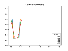
Figure 7: Smoothed Porosity for $\alpha\in\{0.01,0.02,0.04,0.06\}$

We now define error norms for water height $H$ and weighted velocity $uH$ as

$$E_{H} =||H-H_{\alpha}||=\left(\int_{0}^{T}\int_{\Omega}(H-H_{\alpha})^{2}\mathop{}\!\mathrm{d}x\mathop{}\!\mathrm{d}t\right)^{1/2}$$ (109)

$$E_{uH} =||uH-uH_{\alpha}||=\left(\int_{0}^{T}\int_{\Omega}(uH-uH_{\alpha})^{2}\mathop{}\!\mathrm{d}x\mathop{}\!\mathrm{d}t\right)^{1/2}\text{.}$$ (110)

From construction of the well-balanced scheme it is obvious that steady state conditions $uH=0$ for $H+z=C$ lead to zero error norms. We hence exemplifying investigate Gaussian initial conditions for the surface height $H$, i.e. $(H_{0},uH_{0})=(1+0.3\exp(-100(x-1/2)^{2}),0)$, for final time $T=0.4$ and step size $dt={1}\mathrm{e}{-3}$, where the discontinuities are located at $x_{0}=0.038$ and $x_{1}=0.18$. We can observe the convergence numerically, i.e. $U=\lim_{\alpha\rightarrow 0}U_{\alpha}$ for $\phi=\lim_{\alpha\rightarrow 0}\phi_{\alpha}$, as shown in table 1. At this point, we would like to emphasise that the convergence is limited by the grid size of the mesh, hence showing the limit decrease for $\alpha\rightarrow 0$ is only possible for $h_{\kappa}\rightarrow 0$.

$\alpha$	$||H-H_{\alpha}||$	$||uH-uH_{\alpha}||$
0.06	3.45587	8.41055
0.04	2.05134	4.69693
0.03	1.40056	3.08506
0.02	0.81980	1.69824
0.01	0.3443	0.601958
0.005	0.17583	0.23194
0.001	0.10549	0.11108

Table 1: Error Norms $E_{H}$ and $E_{uH}$ for decreasing $\alpha$

References

• [1] Kyung K. Choi. Shape design sensitivity analysis and optimal design of structural systems. In Carlos A. Mota Soares, editor, Computer Aided Optimal Design: Structural and Mechanical Systems, pages 439–492. Springer Berlin Heidelberg, 1987.
• [2] J. Sokołowski and J.P. Zolésio. Introduction to Shape Optimization: Shape Sensitivity Analysis. Springer series in computational mathematics. Springer-Verlag, 1992.
• [3] M. C. Delfour and J. P. Zolésio. Shapes and Geometries. Society for Industrial and Applied Mathematics, second edition, 2011.
• [4] Volker H. Schulz, Martin. Siebenborn, and Kathrin. Welker. Efficient pde constrained shape optimization based on steklov–poincaré-type metrics. SIAM Journal on Optimization, 26(4):2800–2819, 2016.
• [5] Volker Schulz, Martin Siebenborn, and Kathrin Welker. Structured inverse modeling in parabolic diffusion processess. SIAM Journal on Control and Optimization, 53, 09 2014.
• [6] Pascal Azerad, Benjamin Ivorra, Bijan Mohammad, and Frédéric Bouchette. Optimal Shape Design of Coastal Structures Minimizing Coastal Erosion. CIRM, 01 2005.
• [7] Damien Isebe, Pascal Azerad, Frédéric Bouchette, Benjamin Ivorra, and Bijan Mohammadi. Shape optimization of geotextile tubes for sandy beach protection. International Journal for Numerical Methods in Engineering, 74:1262 – 1277, 05 2008.
• [8] Moritz Keuthen and D. Kraft. Shape optimization of a breakwater. Inverse Problems in Science and Engineering, 24, 09 2015.
• [9] Bijan Mohammadi and Afaf Bouharguane. Optimal dynamics of soft shapes in shallow waters. Computers & Fluids, 40:291–298, 01 2011.
• [10] Afaf Bouharguane and Bijan Mohammadi. Minimization principles for the evolution of a soft sea bed interacting with a shallow. International Journal of Computational Fluid Dynamics, 26:163–172, 03 2012.
• [11] Luka Schlegel and Volker Schulz. Shape optimization for the mitigation of coastal erosion via shallow water equations, 2021.
• [12] Adhémar-Jean-Claude Barré de Saint-Venant. Théorie du mouvement non-permanent des eaux, avec application aux crues des rivières et è l’introduction des marées dans leur lit. C. R. Acad Sci Paris, 08 1871.
• [13] Benjamin Dewals, Martin Bruwier, Michel Pirotton, Sebastien Erpicum, and Pierre Archambeau. Porosity models for large-scale urban flood modelling: A review. Water, 13(7), 2021.
• [14] Vincent Guinot and Sandra Soares-Frazão. Flux and source term calculation intwo-dimensional shallow water models with porosity on unstructured grids. International Journal for Numerical Methods in Fluids, 50:309 – 345, 01 2006.
• [15] Brett F. Sanders, Jochen E. Schubert, and Humberto A. Gallegos. Integral formulation of shallow-water equations with anisotropic porosity for urban flood modeling. Journal of Hydrology, 362(1):19–38, 2008.
• [16] Ilhan Özgen, Dongfang Liang, and Reinhard Hinkelmann. Shallow water equations with depth-dependent anisotropic porosity for subgrid-scale topography. Applied Mathematical Modelling, 40(17):7447–7473, 2016.
• [17] Ralf Hartmann. Numerical analysis of higher order discontinuous galerkin finite element methods, 10 2008.
• [18] Yulong Xing and Chi-Wang Shu. A new approach of high order well-balanced finite volume weno schemes and discontinuous galerkin methods for a class of hyperbolic systems with source. Communications in Computational Physics, 1, 02 2006.
• [19] Per-Olof Persson and J. Peraire. Sub-cell shock capturing for discontinuous galerkin methods. AIAA paper, 2, 01 2006.
• [20] Joseph Oliger and Arne Sundström. Theoretical and practical aspects of some initial boundary value problems in fluid dynamics. SIAM Journal on Applied Mathematics, 35(3):419–446, 1978.
• [21] Oksana Guba, Mark Taylor, Paul Ullrich, James Overfelt, and Michael Levy. The spectral element method (sem) on variable-resolution grids: Evaluating grid sensitivity and resolution-aware numerical viscosity. Geoscientific Model Development Discussions, 7, 06 2014.
• [22] Ting Song, Alex Main, Guglielmo Scovazzi, and Mario Ricchiuto. The shifted boundary method for hyperbolic systems: Embedded domain computations of linear waves and shallow water flows. Journal of Computational Physics, 12 2017.
• [23] Grégoire Allaire, François Jouve, and Georgios Michailidis. Thickness control in structural optimization via a level set method. Structural and Multidisciplinary Optimization, 53, 06 2016.
• [24] Juan De los Reyes. Numerical PDE-Constrained Optimization. Springer Cham, 03 2015.
• [25] F.M. Exner. Über die Wechselwirkung zwischen Wasser und Geschiebe in Flüssen. Hölder-Pichler-Tempsky, A.-G., 1925.
• [26] Martin Berggren. A unified discrete-continuous sensitivity analysis method for shape optimization. In CSC 2010, 2010.
• [27] Martin S. Alnæs, Jan Blechta, Johan Hake, August Johansson, Benjamin Kehlet, Anders Logg, Chris Richardson, Johannes Ring, Marie E. Rognes, and Garth N. Wells. The fenics project version 1.5. Archive of Numerical Software, 3(100), 2015.
• [28] Ernst Hairer and Gerhard Wanner. Solving Ordinary Differential Equations II. Stiff and Differential-Algebraic Problems, volume 14. Springer Berlin, Heidelberg, 01 1996.
• [29] Paul Houston and Nathan Sime. Automatic symbolic computation for discontinuous galerkin finite element methods, 2018.
• [30] Vadym Aizinger and Clint Dawson. A discontinuous galerkin method for two-dimensional flow and transport in shallow water. Advances in Water Resources, 25(1):67 – 84, 2002.
• [31] L. Gosse. A well-balanced flux-vector splitting scheme designed for hyperbolic systems of conservation laws with source terms. Computers & Mathematics with Applications, 39(9):135–159, 2000.
• [32] Alfredo Bermudez and Ma Elena Vazquez. Upwind methods for hyperbolic conservation laws with source terms. Computers & Fluids, 23(8):1049–1071, 1994.
• [33] Emmanuel Audusse, Christophe Chalons, and Philippe Ung. A simple three-wave approximate riemann solver for the Saint-Venant–exner equations. International Journal for Numerical Methods in Fluids, 09 2015.
• [34] Christophe Geuzaine and Jean-François Remacle. Gmsh: A 3-d finite element mesh generator with built-in pre- and post-processing facilities. International Journal for Numerical Methods in Engineering, 79:1309 – 1331, 09 2009.
• [35] T. S. Stefanakis, E. Contal, N. Vayatis, F. Dias, and C.E. Synolakis. Can small islands protect nearby coasts from tsunamis? an active experimental design approach. Proceedings of the Royal Society A: Mathematical, Physical and Engineering Sciences, 470(2172):20140575, Dec 2014.
• [36] Alexandros Avdis, Christian Jacobs, Simon Mouradian, Jon Hill, and Matthew Piggott. Meshing ocean domains for coastal engineering applications. In VII European Congress on Computational Methods in Applied Sciences and Engineering, 06 2016.
• [37] V.I. Agoshkov, A. Quarteroni, and F. Saleri. Recent developments in the numerical simulation of shallow water equations i: Boundary conditions. Applied Numerical Mathematics, 15(2):175 – 200, 1994.
• [38] Rafael Correa and Alberto Seeger. Directional derivative of a minmax function. Nonlinear Analysis-theory Methods & Applications, 9:13–22, 01 1985.