Violation of Local Detailed Balance Despite a Clear Time-Scale Separation

Abstract

Integrating out fast degrees of freedom is known to yield, to a good approximation, memory-less, i.e. Markovian, dynamics. In the presence of such a time-scale separation local detailed balance is believed to emerge and to guarantee thermodynamic consistency arbitrarily far from equilibrium. Here we present a transparent example of a Markov model of a molecular motor where local detailed balance can be violated despite a clear time-scale separation and hence Markovian dynamics. Driving the system far from equilibrium can lead to a violation of local detailed balance against the driving force. We further show that local detailed balance can be restored, even in the presence of memory, if the coarse-graining is carried out as Milestoning. Our work establishes Milestoning not only as a kinetically but for the first time also as a thermodynamically consistent coarse-graining method. Our results are relevant as soon as individual transition paths are appreciable or can be resolved.

The formulation of thermodynamic observables, such as heat and work, along individual stochastic trajectories unraveled fundamental fluctuation symmetries which matured into the framework called “stochastic thermodynamics” [1, 2, 3]. In the particular case of continuous-time Markov-jump processes the local detailed balance paradigm emerged, relating the kinetics to thermodynamic forces that drive a system out of equilibrium [4, 5, 2, 3]. One inherent assumption of this paradigm is a separation of timescales [5]: the observed degrees of freedom are slow ensuring that all unobserved/hidden fast degrees of freedom equilibrate with instantaneously connected (heat or particle) reservoirs [3, 6, 7]. Accordingly, the forward and corresponding backward transition rates between a pair of meso-states $A$ and $B$, $w_{A\to B}$ and $w_{B\to A}$, respectively, are related to the entropy production via [8]

$$k_{\rm B}\ln\frac{w_{A\to B}}{w_{B\to A}}=\text{entropy change {\hbox{A\to B}}},$$ (1)

where $k_{\rm B}$ is the Boltzmann constant, and the entropy difference reflects the change of both, the intrinsic entropy and the entropy generated in the reservoirs [5]. However, as soon as slow hidden degrees of freedom emerge (within $A$ or $B$) the exact connection between the observed kinetics and the dissipation embodied in Eq. (1) disappears, which was explained theoretically [9, 10, 11, 12, 13, 14, 15, 16, 17, 18, 19, 20, 21, 22, 23, 24, 25, 26, 27, 28] and corroborated experimentally [29]. The equality (1) can nevertheless be restored under specific conditions [13, 30, 31, 32], using affinities [33], by stalling the system [34, 35] or introducing waiting time distributions [36, 37, 27, 38, 28] that inter alia can further trigger anomalous diffusion [39].

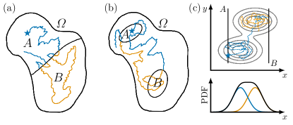
Figure 1: Variants of coarse-graining: the color of the full trajectory evolving from the blue star represent the instantaneous coarse-grained states $A$ (blue) and $B$ (yellow), respectively. (a) State lumping: The full set of states $\varOmega$ is decomposed into subsets $A$ and $B$. (b) Milestoning based on core sets: two metastable states represent the cores $A$ and $B$, and the coarse-grained state corresponds to the last visited core. (c) Top: contour lines depicting potential iso-surfaces in the $xy$ plane; milestones $A$ and $B$ resolve the metastable regions. Bottom: measured equilibrium probability density function (PDF) with the PDFs of the the individual metastable states indicated in blue and orange, respectively.

When the underlying degrees of freedom can assume continuous values any coarse-graining that lumps states as shown in Fig. 1a inherently leads to non-Markovian jump dynamics in continuous time [40, 41] due to fast re-crossings in the transition region between $A$ and $B$. Notably, these can nowadays be experimentally resolved [42, 43, 44, 45, 46, 47] and are therefore important practically. Conversely, Milestoning [48, 49] (see [50, 51, 52] for a broader perspective) turned out to be a coarse-graining scheme that allows for a kinetically consistent mapping of highdimensional dynamics onto a drastically simplified Markov-jump process [41, 53]. The state space is dissected into hypersurfaces which may enclose sub-volumes that are called “cores” [41, 53]. Fig. 1b depicts two such cores $A$ and $B$, whereby the color of the trajectory encodes the last visited core. Beyond a short transient, Markov-jump dynamics emerges from the coarse-graining whenever the trajectory upon leaving any core either (i) quickly returns to it or (ii) quickly transits to the next core [41]. Hereby, condition (i) ensures a local equilibration prior to leaving a state that is required for the emergence of local detailed balance [4, 5, 2, 3]. Besides being kinetically consistent, Milestoning offers two main advantages over lumping.

First, in experiments probing low-dimensional observables one may be able to separate pairs of metastable states even if their projections onto the observable overlap [54]. This is illustrated in Fig. 1c, where two seemingly overlapping metastable states in the projected space $x$ are resolved by choosing the respective milestones outside the overlapping region. Whenever a milestone is left, the trajectory rapidly returns or quickly transits to the other milestone. Thus, the last visited milestone to a good approximation reflects the currently visited metastable region in a possibly higher-dimensional (here 2d) underlying space. Second, we recently discovered that Milestoning naturally ensures local detailed balance in the presence of a time-scale separation [32]. Surprisingly, this extends even to systems without a clear time-scale separation, which we investigate further below. Notably, with so-called “dynamical coring” [55, 54] one can, under certain conditions, convert a “lumped” process into a “milestoned” process by manually discarding short recrossing events as those shown in Fig. 1a.

In contrast to continuous-space processes, the lumping of dynamics that evolve on a discrete state space [2, 3, 4, 8, 9, 10, 12, 13, 14, 15, 16, 17, 18, 19, 20, 21, 22, 23, 27, 30, 31, 36, 37, 38, 34, 35, 7, 6, 28] can in fact yield an effectively Markovian jump process. According to perturbation theory Eq. (1) is satisfied by lumped-state dynamics in the limit of an infinite time-scale separation [15], which was corroborated in [18, 19, 21]. This general belief was, however, never systematically scrutinized in practice.

In this Letter we show, by means of a simple yet biophysically relevant example, that time-scale separation surprisingly and against common belief does not ensure the existence of local detailed balance. The minimum time-scale separation required for Eq. (1) to hold may grow exponentially with the thermodynamic driving force. In other words, time-scale separation may not suffice arbitrarily far from equilibrium. Milestoning, in stark contrast to lumping (see Fig. 1), robustly ensures local detailed balance in the limit of a time-scale separation. This result indicates that unlike lumping, Milestoning generically yields a thermodynamically consistent coarse-graining.

$F_{1}$-ATPase driven far from equilibrium.—We consider the molecular motor F₁-ATPase driven by the hydrolysis of adenosine triphosphate (ATP). The dynamics evolves as a Markov processes on six rotational states [56] as shown in Fig. 2a: The binding of ATP occurs with a rate $\kappa_{+}$ proportional to the concentration of ATP and effetcs a $90^{\circ}$ rotation. The reverse unbinding occurs with the rate $\kappa_{-}$. ATP hydrolisis to ADP is assumed to be infinitely fast. The release of ADP occurs with rate $\omega_{+}$ and triggers a $30^{\circ}$ rotation, and the reverse step occurs with rate $\omega_{-}$.

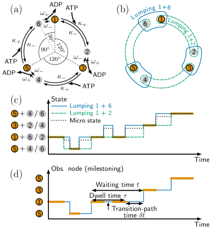
Figure 2: Model and coarse-graining. (a) Full six state model; the dotted lines denote odd rotational states $\{1,3,5\}$ (orange) separated by $120^{\circ}$. The even intermediate states (gray) separate each rotation step into $90^{\circ}$ and $30^{\circ}$ substeps. (b) Two types of lumping; the solid boxes “lumping 1+6” lump states $\{1,6\}$, $\{2,3\}$, and $\{5,6\}$, respectively, whereas the dashed boxes “lumping 1+2” lump states $\{1,2\}$, $\{3,4\}$, and $\{5,6\}$. (c) Coarse-grained trajectory using “lumping 1+2” and “lumping 1+6”; the orange segments represent visits of odd states. The dotted line (“micro state”) indicates the rotational state of the motor as function of time. (d) Coarse-grained trajectory deduced from Milestoning; the milestones are placed at odd states.

The free energy $\mu$ liberated by the hydrolysis of one $\text{ATP}\to\text{ADP}$ at a given concentration relates to the entropy change times the temperature $T$, and local detailed balance (1) imposes

$$k_{\rm B}T\ln\frac{\omega_{+}\kappa_{+}}{\omega_{-}\kappa_{-}}=\mu.$$ (2)

Heneceforth we measure energies, $\mu$, in units of the thermal energy $k_{\rm B}T$. The steady state probability to find the ATPase in even and odd states is given by [57]

$$P_{\rm odd}=\frac{\omega_{+}+\kappa_{-}}{\omega+\kappa}\quad\text{and}\quad P_{\rm even}=\frac{\omega_{-}+\kappa_{+}}{\omega+\kappa},$$ (3)

respectively, where we defined $\kappa\equiv\kappa_{+}+\kappa_{-}$ and $\omega\equiv\omega_{+}+\omega_{-}$. The entropy production rate can be expressed with the rate of ATP consumption, $J=P_{\rm odd}\kappa_{+}-P_{\rm even}\kappa_{-}$, via [57]

$$\sigma=J\mu.$$ (4)

This completes the description of the “full” system.

Lumping.—We now perform a coarse-graining to reduce the six states to three. Two sensible ways to lump the states are shown in Fig. 2b. Assuming Markovian dynamics the effective forward “$+$” and backward “$-$” rates on the lumped space read [15]

$$W^{1+6}_{\pm} =P_{\begin{subarray}{c}\text{odd}\\ \text{even}\end{subarray}}\kappa_{\pm}=\frac{(\omega_{\pm}+\kappa_{\mp})\kappa_{\pm}}{\kappa+\omega},$$ (5)

$$W^{1+2}_{\pm} =P_{\begin{subarray}{c}\text{even}\\ \text{odd}\end{subarray}}\omega_{\pm}=\frac{(\omega_{\mp}+\kappa_{\pm})\omega_{\pm}}{\kappa+\omega},$$

and satisfy $J=W^{1+6}_{+}-W^{1+6}_{-}=W^{1+2}_{+}-W^{1+2}_{-}$. In terms of effective rates the coarse-grained entropy reads [15]

$$\tilde{\sigma}_{z}=J\ln\frac{W^{z}_{+}}{W^{z}_{-}},$$ (6)

with $z=1+6$ or $z=1+2$ and using Eqs. (4-6) yields

$$\frac{\tilde{\sigma}_{1+6}}{\sigma} =1-\frac{1}{\mu}\ln\frac{1+{\rm e}^{\mu}\kappa_{-}/\omega_{+}}{1+\kappa_{-}/\omega_{+}},$$ (7)

$$\frac{\tilde{\sigma}_{1+2}}{\sigma} =1-\frac{1}{\mu}\ln\frac{1+{\rm e}^{\mu}\omega_{-}/\kappa_{+}}{1+\omega_{-}/\kappa_{+}}.$$ (8)

Both ratios (7) and (8) are positive and bounded by $1$ [15], i.e., $\tilde{\sigma}_{z}\leq\sigma$ (see also [58]).

Time-scale separation.—In agreement with [15] (see also [18, 19, 21]) in the limit $\kappa_{-}\ll{\rm e}^{-\mu}\omega_{+}$ (i.e., $\kappa\to 0$) we obtain $\tilde{\sigma}_{1+6}\approx\sigma$, whereas the limit $\omega_{-}\ll{\rm e}^{-\mu}\kappa_{+}$ (i.e., $\omega\to 0$) yields $\tilde{\sigma}_{1+2}\approx\sigma$. In other words, when hidden jumps are much faster than those between lumped states, the coarse-grained dynamics are approximately Markovian and preserve the entropy production.

A time-scale separation is manifested as a gap in the spectrum of the Markov generator, which separates fast from slow modes (see Part II in [59]). In our model $\kappa\gg\omega$ and $\kappa\ll\omega$ are the only kinds of time-scale separation, and in principle require two different types of lumping (for details see ). At high ATP concentration ($\kappa\gg\omega$) “lumping $1+2$” (see dashed boxes in Fig. 2b) hides the fast degrees freedom $\sim\kappa$. Conversely, at low ATP concentration one should rather lump $1+6$ (see solid boxes in Fig. 2b). Note that whenever the entropy production rate is deduced from a master equation [2, 3, 4, 8, 9, 10, 12, 13, 14, 15, 16, 17, 18, 19, 20, 21, 22, 23, 27, 30, 31, 36, 37, 38, 34, 35, 7, 6, 28] one explicitly (or implicitly) assumes the observed degrees of freedom to be formally infinitely slower than any possibly hidden ones.

Violation of local detailed balance.—In practice an infinite time-scale does not exist and the driving $\mu$ becomes important if it substantially exceeds the thermal energy ($\mu\gg 1$), which in turn implies ${\rm e}^{\mu}\ggg 1$. To see this set $\omega_{\pm}$ and $\kappa_{-}$ to be constant while varying the ATP concentration as $\kappa_{+}\propto e^{\mu}$ as in [56] (the parameters are given in Fig. 3). For $\mu<10$ we find $\omega\gg\kappa$ and as expected $\tilde{\sigma}_{1+6}\approx\sigma$ (see Fig. 3). For $\mu>15$ we have $\omega\ll\kappa$, however, to our surprise $\tilde{\sigma}_{1+2}\not\approx\sigma$ (because $\omega_{-}\not\ll{\rm e}^{-\mu}\kappa_{+}$). Inspecting Eq. (7) we actually find $\tilde{\sigma}_{1+2}\approx 1-10/\mu$ (see Fig. 3a). Thus one obtains $\tilde{\sigma}_{1+2}/\sigma\to 1$ in the limit $\mu\to\infty$, which is approached algebraically slowly. For example, in the already unphysical situation $\mu=40\,k_{\rm B}T$ only $75\,\%$ of the entropy production are recovered in Eq. (6). Moreover, at physiological conditions $\mu=20$ we find a clear time-scale separation, $\kappa/\omega\approx 140\gg 1$ [see $\lambda_{1}$ and $\lambda_{2}$ in Eq. (9) for the precise time-scales],, yet the entropy production is not even remotely restored. This surprising finding is the first main result of this Letter.

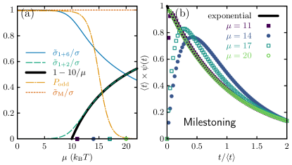
Figure 3: Entropy production and waiting time statistics with Milestoning. (a) Entropy production, $\tilde{\sigma}_{1+6}$ and $\tilde{\sigma}_{1+2}$ deduced from the lumpings “1+6” and “1+2”, respectively. The thick line depicting $1-10/\mu$ approaches $\tilde{\sigma}_{1+2}/\sigma$ in the limit $\mu\to\infty$. The dash-dotted yellow line denotes the steady state probability $P_{\rm odd}$. (b) Probability density of waiting time $t$ (see Fig. 2d) for $\mu$ values indicated in (a). The thick black line depicts an exponential density $\propto{\rm e}^{-t/\langle t\rangle}$. Parameters: $\omega_{+}=1$, $\omega_{-}={\rm e}^{-5}$, $\kappa_{+}={\rm e}^{\mu-15}$, and $\kappa_{-}={\rm e}^{-10}$.

How can we reconcile this? For convenience we focus on $\mu=20$ and the lumping “1+2”, which in fact represents a semi-Markov process of second order [36] (see also [37, 27, 38]). That is, the waiting time density $\psi_{\pm|\pm}(t)$ depends on both, the previous and next visited state with the normalization $\int_{0}^{\infty}[\psi_{+|i}(t)+\psi_{-|i}(t)]dt=1$ and $i=\pm$. In particular, for the given parameters we find

$$\begin{pmatrix}\psi_{+|+}(t)\!&\psi_{+|-}(t)\\ \psi_{-|+}(t)\!&\psi_{-|-}(t)\end{pmatrix} \!\approx\!\begin{pmatrix}1.007&1.000\\ 2.089\cdot 10^{-9}&2.075\cdot 10^{-9}\end{pmatrix}{\rm e}^{-\lambda_{1}t}$$

$$+ \begin{pmatrix}-1.007&3.100\cdot 10^{-7}\\ 6.738\cdot 10^{-3}&-2.075\cdot 10^{-9}\end{pmatrix}{\rm e}^{-\lambda_{2}t},$$ (9)

where $\lambda_{1}\approx 1.0{\color[rgb]{0,0,0}{}\approx\omega}$ and $\lambda_{2}\approx 148.4{\color[rgb]{0,0,0}{}\approx\kappa}$. The analytical expression for the waiting time density is immaterial for the present discussion but straightforward to determine. For times $t\gtrsim 0.15$ the jumps are essentially Markovian – the waiting time density is to a good approximation exponential and independent of the previous step, $\psi_{\pm|+}\approx\psi_{\pm|-}$, and the fast decaying mode is negligible, ${\rm e}^{-\lambda_{2}t}\approx 0$. Remarkably, using Eq. (9) one finds $\ln[\psi_{+|i}(t)/\psi_{-|i}(t)]\approx\mu=20$ for for all $t\gtrsim 0.15$ and $i=\pm$. Hence, only short times $t\leq 0.15$ encode a violation of Markovianity and broken local detailed balance. At strong driving most of the jumps occur in positive direction “$+$” and on average take equally long $\approx 1/\lambda_{1}\approx 1$. In fact, only the backward jump “$-$” can be faster on average, however, if and only if the preceding jump occurred in the forward “$+$” direction, i.e. a forward transition is followed immediately by a backward transition. In this case one finds $\int_{0}^{\infty}t\psi_{-|+}(t)dt/\int_{0}^{\infty}\psi_{-|+}(t)dt\approx 0.0067\approx 1/\lambda_{2}$. These rare events lead to an “overestimation” of the effective backward transition rate $W_{-}^{1+2}\gtrsim\omega_{-}\kappa_{+}/\kappa$. Note that a locally equilibrated backward rate would need to satisfy $\ln(W_{-}^{1+2})\approx\ln(\omega_{-}\kappa_{+}/\kappa)$, which is satisfied if in addition to the time-scale separation the individual rates satisfy $\kappa_{\pm}\gg\omega_{\pm}$ (see, e.g., [15]).

By evaluating exactly the waiting time distribution to include the short-time behavior one is able to restore the entropy production from the two-step affinity via [36]

$$\sigma_{\rm aff}^{1+2}=J\ln\frac{\int_{0}^{\infty}\psi_{+|+}(t)dt}{\int_{0}^{\infty}\psi_{-|-}(t)dt}=J\mu,$$ (10)

where the last equality follows from Eqs. (2) and (9) (here $\mu=20$). Thus, by taking into account the tiny non-Markovian features in Eq. (9) one can in principle recover the entropy production. This, however, poses a serious practical problem at strong driving $\mu\gg 1$. Namely, to deduce Eq. (10) from an experiment we formally require a trajectory with statistically sufficiently many incidents of finding two consecutive backward steps not interrupted by a forward step. It thus seems that one is required to reliably observe rare events with a probability $\propto({\rm e}^{-\mu})^{2}$, which may not be feasible.

In the following we illustrate how an alternative coarse-graining – Milestoning – effectively restores Markovian dynamics in a thermodynamically consistent manner while it concurrently effectively squares the sample size by relying only on the evaluation of single rare backward jumps that occur with probability $\approx{\rm e}^{-\mu}$.

Thermodynamic consistency of Milestoning.—We define three milestones (or cores) at locations highlighted by dotted black lines in Fig. 1a. These represent the three odd rotational states. We measure the passages across the milestones (see thick yellow lines in Fig. 1c). If the angle were measured continuously, the passages through the milestones would correspond to instantaneous events [32]. The coarse-grained process at any time reflects the last visited Milestone (see blue line). As in Ref. [32] we dissect waiting times into the dwell and transition time periods. The dwell time represents all loops returning to the original milestone, while the transition-path time reflects the time of commuting between milestones. The waiting time can be shown to be the sum of the statistically independent dwell and transition-path times (see second main result in [32]). The main advantage of this decomposition is that the statistics of transition-path time encode information about potentially hidden multidimensional pathways [62] (see also [63, 32, 64]).

If the gaps between revisitations of the same milestone (see vertical arrow in Fig. 1d) and transition-path times are negligibly short compared to the waiting time in a state, the resulting “Milestoned process” becomes, to a good approximation, Markovian [41]. Note that milestones may represent closed (see [41] and Fig. 1b) or open (see [48, 49] and Fig. 1c) hypersurfaces.

Let $\phi_{\pm}$ denote the splitting probability that the next milestone will be visited in the forward “$+$” and backward “$-$” direction, respectively. One can confirm (cf. first main result in [32]) that

$$\ln\frac{\phi_{+}}{\phi_{-}}=\ln\frac{\kappa_{+}\omega_{-}}{\kappa_{-}\omega_{-}}=\mu$$ (11)

holds. That is, Milestoning transition probabilities exactly encode the entropy production per hydrolyzed ATP.

Since transition-path times obey a reflection symmetry [65] and because the dwell time statistics do not depend on the exit direction [32] the waiting time densities in the $+$ and $-$ direction coincide, i.e. $\psi_{\pm}(t)=\psi(t)$. In the presence of hidden dissipative mechanisms the symmetry may be lifted counterintuitively [66, 67]. Denoting the mean waiting time by $\langle t\rangle=\int_{0}^{\infty}t\psi(t)dt$, the steady state current becomes $J^{\rm M}=\phi_{+}/\langle t\rangle-\phi_{-}/\langle t\rangle=J$. Defining the Milestoning rates as $W^{\rm M}_{\pm}=\phi_{+}/\langle t\rangle$ and inserting them into Eq. (6) yields, using Eqs. (4) and (11), $\tilde{\sigma}_{\rm M}=\sigma$. Thus, Milestoning in contrast to lumping preserves the entropy production in the limit of a time-scale separation and beyond.

Upon inspecting the waiting time density we find that it is to a good approximation memory-less for $\mu\lesssim 10$ as well as for $\mu\gtrsim 20$, while the non-exponential behavior is most pronounced in the regime $10\leq\mu\leq 20$ (see Fig. 3b). Thus, in the limit of either of the two time-scale separations, $\mu\lesssim 10$ and $\mu\gtrsim 20$, the Milestoned dynamics is to a good approximation Markovian. In contrast to lumping, Milestoning restores local detailed balance (1) in both directions, parallel and anti-parallel to the driving, even at large asymmetries, which is the second main result of this Letter.

Notably, the regime $\mu\lesssim 10$ clearly fulfills both criteria (i) and (ii) for the emergence of Markovian dynamics [41] if the probability to reside within a core satisfies $P_{\rm odd}\approx 1$. Conversely, the opposite limit $\mu\gtrsim 20$ does not obviously imply Markovian kinetics. To understand why it does so nevertheless, we point out that in this limit (a) $P_{\rm even}=1-P_{\rm odd}\approx 1$. If we were to choose the even (gray) states as cores instead of the odd (yellow) ones (see Fig. 2a), we would obviously restore the criteria for the emergence of Markovian dynamics [41]. It turns out further that (b) the waiting time density remains unaffected by the exchange of $\omega_{\pm}$ and $\kappa_{\pm}$, i.e. it does not depend on whether we choose the odd or even states as milestones. This explains why an exponential distribution emerges to a good approximation also in the limit $\mu\gtrsim 20$. We also note that the kinetic hysteresis discovered in [32] almost vanishes as soon as Markovian dynamics emerge and the aforementioned criteria [41] are satisfied, which here follows from (a) by choosing the even states as milestones.

Conclusion.—We have shown that a clear time-scale separation, in contrast to the common belief, is only a necessary but not a sufficient condition for the validity of local detailed balance. By coarse-graining a detailed Markov model of a strongly driven molecular motor we demonstrated a clear time-scale separation between the observed and hidden degrees of freedom and hence Markovian dynamics of the observable, and concurrently the non-existence of a local equilibrium against the driving. Our work demonstrates, for the first time, that Milestoning restores thermodynamic consistency in the steady state in the presence of strong driving even if the dynamics displays memory. A coarse-graining based on lumping may yield effectively Markovian dynamics that nevertheless violates local detailed balance. It will be interesting to revisit recent works on the thermodynamics of systems with slow hidden degrees of freedom that employed lumping [36, 37, 27, 38] to inspect if and how these change under the thermodynamically consistent Milestoning which will lead to correlated transitions [68] and/or dwell times [32]. Beyond the examples shown here as well as in Sec. II of [60] it will be interesting to investigate whether the two conditions for Markovianity together with Milestoning [41] generally guarantee the validity of local detailed balance.

Acknowledgments. The financial support from the German Research Foundation (DFG) through the Emmy Noether Program GO 2762/1-2 to A. G. is gratefully acknowledged.

Supplemental Material

I Time-scale separation in the ATPase model

I.1 General discussion

The time-scale separation emerges if any of the two clusterings “Lumping 1+2” or “Lumping 1+6” have meso-states that relax much faster than the remaining transitions. Since two-level systems relax to equilibrium with a rate that is roughly given by the sum of both rates connecting the two states, we obtain a time-scale separation as soon as either $\omega\ll\kappa$ or $\omega\gg\kappa$, which we explain more thoroughly in the following.

Without loss of generality we focus on “Lumping 1+2” (see Fig. 2b in the main text) and rationalize why $\kappa\gg\omega$ actually corresponds to a proper separation of time scales. The other time-scale separation associated with “Lumping 1+6” and $\omega\gg\kappa$ follows by analogy, which is mathematically obtained by interchanging $\omega_{\pm}\leftrightarrow\kappa_{\pm}$ in the discussion below.

The dynamics inside a mesostate $1+2$ (see Fig. 2b in the main text) occurs with “internal” rates $\kappa_{\pm}$ within the lumped-states. The lumped states are exited either with rate $\omega_{-}$ from state $1$ (odd numbered) or with rate $\omega_{+}$ from state $2$ (even numbered). The eigenvalues of the Generator within one lumped state represent the zeros of the characteristic polynomial

$$\chi(\lambda)=\det\begin{pmatrix}\lambda+\kappa_{+}+\omega_{-}&-\kappa_{-}\\ -\kappa_{+}&\lambda+\kappa_{-}+\omega_{+}\end{pmatrix}$$ (12)

which leads to the eigenvalues

$$\lambda_{\pm}=\frac{\omega+\kappa}{2}\pm\sqrt{\Big{(}\frac{\omega+\kappa}{2}\Big{)}^{2}-C},$$ (13)

where $\omega\equiv\omega_{+}+\omega_{-}$, $\kappa\equiv\kappa_{+}+\kappa_{-}$ and $C\equiv\omega_{+}\kappa_{+}+\omega_{-}\kappa_{-}+\omega_{+}\omega_{-}$. In the main text we set $\lambda_{2}=\lambda_{+}$ and $\lambda_{1}=\lambda_{-}$. The two relaxation time scales are $1/\lambda_{+}$ and $1/\lambda_{-}$, which correspond to the two-scale exponential decay due to the two states within one meso-state. In general, lumping $n$ states will lead to $n$ exponentially decaying modes. A separation of time scale demands that all dynamical modes except for one exponentially decaying mode are quickly relaxing (here $\lambda_{+}\gg\lambda_{-}$ or $1\gg\lambda_{-}/\lambda_{+}$). We relate this condition to the rates via

$$1 \stackrel{{\scriptstyle!}}{{\gg}}\frac{\lambda_{-}}{\lambda_{+}}=\frac{\lambda_{-}\lambda_{+}}{\lambda_{+}^{2}}\simeq\frac{\lambda_{-}\lambda_{+}}{(\lambda_{+}+\lambda_{-})^{2}}$$

$$=\frac{\omega_{+}\kappa_{+}+\omega_{-}\kappa_{-}+\omega_{+}\omega_{-}}{(\omega+\kappa)^{2}}\equiv R,$$ (14)

where in the last step of the first line we self-consistently re-used the first inequality implying $\lambda_{+}\simeq\lambda_{+}+\lambda_{-}=\omega+\kappa$, and the very last step defines the ratio $R$. In other words, time-scale separation for “Lumping 1+2” demands $R\ll 1$. Let us now test whether (and when) this condition is satisfied in our model.

I.2 Testing the time-scale separation in the model

Defining $p\equiv\kappa_{-}/\kappa$ and $q\equiv\omega_{-}/\omega$, which both satisfy $0\leq p,q\leq 1$, the ratio (14) becomes

$$R=\frac{[(1-p)(1-q)+pq]\omega\kappa+q(1-q)\omega^{2}}{(\omega+\kappa)^{2}}.$$ (15)

If $\kappa\gg\omega$ we find $R\approx[(1-p)(1-q)+pq]\omega\kappa^{-1}\ll 1$, which using $q\approx 0.0067\ll 1$ from the parameter given in Fig. 3 in our case yields $R\approx(1-p)\omega/\kappa\leq\omega/\kappa$. Thus $\kappa\gg\omega$ clearly implies a separation of time scales, i.e., $R\ll 1$, which is further “strengthened” due to $(1-p)<1$. In other words, $\kappa\gg\omega$ implies that all internal modes relax much faster than the slowest one, which reflects a memoryless exponential decay. This completes the proof that $\kappa\gg\omega$ in fact implies a separation of time scales $\lambda_{+}\gg\lambda_{-}$ for Lumping $1+2$. Note that we have determined in Eq. (9) in the main text the time-scale separation $R=\lambda_{1}/\lambda_{2}\equiv\lambda_{+}/\lambda_{-}\simeq 1/148$ that is actually stronger than $\omega/\kappa\simeq 1/140$.

I.3 Spectral criterion for time-scale separation

For the sake of completeness we discuss the time-scale separation also in a slightly alternative (but equivalent) interpretation using the spectrum of the Markov generator [69, 59] (see also Ref. [70] for recent related work on local detailed balance). In this setting we consider the full system (in our case the six-state system from Fig. 2(a) in the main text). For simplicity we focus on the specific example with parameters given in Fig. 3 and $\mu=20$, which is also used in Eq. (9) in the main text. Inserting all the rates in the full six-state system leads to to six eigenvalues, where $\lambda_{0}=0$ corresponds to the steady state distribution that does not change with time. The other five eigenvalues are $\lambda_{1,2}\approx 1.5\pm 0.88\,{\rm i},\lambda_{3,4}\approx 147.9\pm 0.88\,{\rm i}$, $\lambda_{5}=149.4$. Consistent with the previous discussion these values confirm the gap in the eigenvalue spectrum $0=\mathrm{Re}(\lambda_{0})\leq\mathrm{Re}(\lambda_{1})\leq\mathrm{Re}(\lambda_{2})\ll\mathrm{Re}(\lambda_{3})\leq\mathrm{Re}(\lambda_{4})\leq\mathrm{Re}(\lambda_{5})$, i.e., three eigenmodes ($0^{\rm th}$-$2^{\rm nd}$ eigenvalue) relax much slower with a rate $\leq 1.5$ than the other three (3rd-5th eigenvalue) with a rate $\geq 149.4$. We thus confirm the time-scale separation by means of the definition given in Ref. [69]. More generally, we explicitly illustrate in Fig. 4 the size of the gap between the second and third mode as function of the driving $\mu$, which except for $\mu\sim 15$ is in fact always quite pronounced.

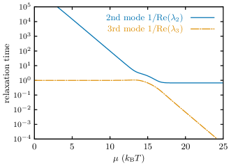
Figure 4: Relaxation time of second and third eigenmode as function of the driving $\mu$.

Note that a (coarse-grained) three-state Markov model can account only of three eigenvalues $\lambda_{0},\lambda_{1},\lambda_{2}$ (and hence time scales) and their corresponding eigenfunctions. If more time scales are required/desired one must increase the number of states.

I.4 Pecularity of the violation of local detailed balance

In Eq. (9) in the main text we evaluate the waiting time in the coarse-grained state given that the next move and preceding moves are heading in either of both directions ($+$ or $-$), respectively. Inspecting said waiting time density one immediately finds that local detailed balance is satisfied, to a very good approximation, if the second term is ignored. Thus, the second term alone encodes the violation of local detailed balance.

Since the second term decays much faster than the first term ($\lambda_{2}\gg\lambda_{1}$) most state-changes occur after an effective local equilibration. There is just one sequence of events that is able to avoid a clear local equilibration. Namely that involving the forward jump “$+$” followed by the backward jump “$-$”, which is the only sequence of transitions that allow the prefactor of the second term to outweigh the first one. More precisely, using Eq. (9) in the main text the corresponding waiting time density reads $\psi_{-|+}(t)=2.089\cdot 10^{-9}{\rm e}^{\lambda_{1}t}+6.738\cdot 10^{-3}{\rm e}^{\lambda_{2}t}$ with $6.738\cdot 10^{-3}\gg 2.089\cdot 10^{-9}$. Thus, after a short time $t\ll 0.15$, (i.e., much shorter than 15,% of the mean waiting time) we find a violation of local equilibration, whereas for $t\geq 0.15$ a local equilibration is established, that is, $\psi_{-|+}(t)\approx 2.089\cdot 10^{-9}{\rm e}^{\lambda_{1}t}$. Therefore, the violation of local detailed balance leading to $\tilde{\sigma}_{1+2}/\sigma<1$ in Fig. 3a (for $\mu=20$) is caused almost entirely by the forward jumps ($+$) that are followed by a backward jump ($-$) which are shorter than 15 % of the total mean waiting time.

Since backward transitions are extremely rare at $\mu=20$, we find that most transitions $>99.9\,\%$ occur upon a local equilibration.

Note that there are several other variants where local equilibration is manifested. For example, using Eq. (3) in the main text one finds $P_{\rm even}\approx\frac{\kappa_{+}}{\kappa}\equiv P_{\rm even}^{\text{eq}}$ whereas $P_{\rm odd}\not\approx 1-\frac{\kappa_{+}}{\kappa}=\frac{\kappa_{-}}{\kappa}=P_{\rm odd}^{\text{eq}}$. The second line in Eq. (5) implies that the forward transitions are sampled from local equilibrium $W_{+}^{1+2}\approx P_{\rm even}^{\text{eq}}\omega_{+}$ but $W_{-}^{1+2}\not\approx P_{\rm odd}^{\text{eq}}\omega_{-}$. Thus, local equilibration sets in before each forward transition but not before backward transitions.

It is worth mentioning that if in addition to the time-scale separation all individual transitions satisfy the mathematical stronger condition $\kappa_{+},\kappa_{-}\gg\omega_{+},\omega_{-}$ one restores local detailed balance in both directions (e.g., see Ref. [15]). In the following we discuss prominent examples from diffusion models which can never satisfy this stronger condition.

II Kramers’ theory and local detailed balance

In systems with continuous coordinates (for example, in any biophysical system) Markov-jump processes in the continuous-time limit (i.e., short lag-time limit) are well-known to not follow from a coarse-graining that is based on lumping [40, 41] [see also paragraph after Eq. (2.47) in Ref. [69]]. In fact, we argue that local detailed balance may not exist if the coarse-graining is based solely on lumping. To see this we re-investigate below Kramers’ original work [71] (see also Ref. [72] for a review), which pioneered the microscopic understanding of local detailed balance and, more precisely, the constituents which are the rate velocities akin to transition rates. In stochastic thermodynamics Kramers’ microscopic understanding is routinely used (directly or implicitly) to model stochastic pumps (cf. Arrhenius rates) [73, 74, 75], stochastic resonance [76], occasionally for kinetic proofreading [77, 78], and many others.

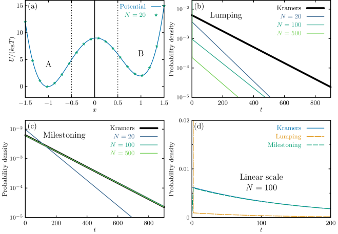
Figure 5: Testing Kramers’ theory with a tilted double-well potential. (a) Potential (solid blue line) and its discrete finite element (Markov state) representation with $N=20$ states. The vertical solid line separates the potential into lumped states A and B. Milestoning is represented by the two vertical dotted lines within states A and B, where the region between the dotted lines can belong to either A or B (depending on which dotted line was crossed last). (b) Waiting time density in state B predicted by Kramers $\wp_{{\rm B}\to{\rm A}}=w_{\rm BA}{\rm e}^{-w_{\rm BA}t}$ using Eq. (18) versus waiting time density to stay on the right half of the potential (vertical solid line in (a)) for $N=20,100,500$ grid-points. (c) First passage time density to pass the left dotted line at $x=-0.5$ for the first time if the particle starts right of the vertical dotted line at $x=0.5$ in (a), which represents the waiting time density in B based on Milestoning if the milestones are chosen by the vertical dotted lines in panel (b). The thick line represents Kramers theory from (b). (d) Direct comparison of Kramers theory with Lumping and Milestoning with a finite element method and $N=100$ states. In the limit $N\to\infty$ Lumping leads to delta distribution of the probability density with the probability weight moving to $t=0$.

In the following we rationalize why Kramers’ theory [71, 79] is incompatible with lumping in continuous time processes. To illustrate this we consider a particle at position $x$ in a tilted double-well potential

$$\frac{U(x)}{k_{\rm B}T}=8*(x+1)^{2}+(x-1)^{2}+x,$$ (16)

where the last term introduces the tilt. The potential is illustrated in Fig. 5a, where the vertical solid line separates the two lumped meso-states which include the minima A and B (the vertical dotted lines will be used for Milestoning below). The tilt leads to a free energy difference between right state B and left state A to be given by $\approx 2\,k_{\rm B}T$.

To use Kramers’ theory we determine the location of two minima of the potential (16) at $x_{\rm A}\approx-1.01527$ and $x_{\rm B}\approx 0.983993$ alongside the local maximum at $x_{\rm max}=0.0312806$. For an overdamped particle with diffusion constant set to unity $D=1$ and $k_{\rm B}T\equiv 1$ Kramers’ work predicts the rates to be approximately given by [71, 79]

$$w_{{\rm A}\to{\rm B}} =\frac{\sqrt{U^{\prime\prime}(x_{\rm A})U^{\prime\prime}(x_{\rm max})}}{2\pi}{\rm e}^{U(x_{\rm A})-U(x_{\rm max})}$$

$$\approx 8.8689\times 10^{-4}$$ (17)

and

$$w_{{\rm B}\to{\rm A}} =\frac{\sqrt{U^{\prime\prime}(x_{\rm B})U^{\prime\prime}(x_{\rm max})}}{2\pi}{\rm e}^{U(x_{\rm B})-U(x_{\rm max})}$$

$$\approx 6.2510\times 10^{-3},$$ (18)

where $U^{\prime\prime}(x)\equiv\partial_{x}^{2}U(x)$ is the second derivative that relates to the curvature of the potential. In the following we test Kramers’ result first against lumping and then against Milestoning.

II.1 Lumping is inconsistent with Kramers’ theory

Let us first test Lumping against Kramers’ rates. To test this numerically we use a thermodynamically consistent finite element method from [80] which we also used in [81] to derive local time distribution for diffusion processes. To this end we discretize our potential in $N$ steps. The discretization $i=1,\ldots,N$ for $N=20$ is shown in Fig. 5a (see green symbols). For convenience we confine the grid between equidistant points $x_{1}=-1.5$ and $x_{N}=1.5$ with a grid spacing $dx=x_{i+1}-x_{i}=(x_{N}-x_{1})/(N-1)=3/(N-1)$. The finite-element method (FEM) is chosen to represent a Markov-jump process between the states $i$ and $j=i\pm 1$ for any $1\leq i,i\pm 1\leq N$ to be given by [80] (see also [81])

$$w_{i\to i\pm 1}^{\rm FEM}=\frac{D}{(dx)^{2}}\exp\left[\frac{U(x_{i})-U(x_{i\pm 1})}{2k_{\rm B}T}\right],$$ (19)

where we set $D=k_{\rm B}T=1$.

To evaluate the waiting time in B for a given grid with $N$ states based on lumping we measure the waiting time of the process until the right half of the potential (right of vertical dotted line in Fig. 5a) is left for the first time after entering said region. Using the rates from Eq. (19) leads to the waiting time density in Fig. 5b for $N=20,100,500$. The following two observations can be made.

First, the waiting time distribution becomes shifted towards shorter times as $N$ increases, which we mathematically expect, since any overdamped diffusion process (i.e., $N\to\infty$) formally “wriggles” infinitely often across any position it visits, which in turn leads to vanishingly short waiting times in the limit $N\to\infty$. Note that even underdamped systems can wriggle several times across a barrier, which is typically accounted for by the success probability to “actually” cross the barrier also called the “transmission coefficient” (e.g., see Ref. [50]). It is worth mentioning that we believe that “Dynamical coring” [55, 54] tackles this problem by effectively removing all the fast fast re-crossings, which means the waiting time density then approximately selects the rate of the long time tail of the lumped process.

Second, excluding the fast re-crossings and focusing on the long-time limit we find a non-normalized exponential decay that is faster than Kramers’ result, which is due to the fact that any lumped state “senses” only one half of the barrier’s curvature which enters Eqs. (17) and (18). The full curvature requires a full crossing of the barrier, which we discuss below in more detail whilst discuss Milestoning. Note that Fig. 5b shows the probability density on a semi-log-scale, which renders exponential decays to straight lines. See Fig. 5d for the linear-scale plot with $N=100$, which also includes Milestoning that is discussed in the following subsection.

These aforementioned two aspects the (re-crossing and half of barrier sampling) are the key reasons why Kramers’ theory is fundamentally incompatible with lumping. Note that we are not the first to show this incompatibility, since it follows from several previous findings, which can in particular be drawn from the paragraph following Eq. (2.47) in Ref. [69] and is also mentioned in Refs. [40, 41] to name but a few. In contrast to our work pursued the main text, this conflict arises merely from projecting a continuous space dynamics into discrete one, which we also pointed out in our recent work [32].

II.2 Milestoning in Kramers’ theory

Let us now study Kramers’ rate theory in the context of Milestoning. To this end we locate the two milestones at $x=-0.5$ (A) and $x=0.5$ (B) (see vertical dotted lines in Fig. 5a). The coarse-graining that is based on Milestoning simply maps the full dynamics into the last crossed milestone. Thus, for any $x\leq-0.5$ the coarse-grained state is “A” and for any $x\geq 0.5$ the state is mapped to “B”, whereas for any $-0.5\leq x\leq 0.5$ the process is mapped to either “A” or “B”, depending on which milestone was passed last. Note that we start to record the coarse-grained state as soon as the first milestone is crossed. One waiting time interval in state B corresponds to the time between the first entrance into B by crossing $x=0.5$ until the other milestone A at $x=-0.5$ is crossed for the first time.

To measure the waiting time we use the finite element method from Eq. (19). To deduce the waiting time density in state B we use the grid state of the right dotted line ($x=0.5$) as the starting condition and the state left of the left dotted line ($x=-0.5$) as the target or absorbing condition. The resulting waiting-time density is shown in Fig. 5c. We find for $N\gtrsim 20$ that the waiting time density to a good approximation approaches the waiting time density predicted by Kramers approximation, i.e., Arrhenius law. We show the waiting time density for $N=100$ in Fig. 5d on a linear scale (see Milestoning and Kramers). For completeness we show the mean values of the waiting time including the reverse transition ${\rm A}\to{\rm B}$ in Tab. 1. One can see that the mean waiting time determined by Milestoning approximates the Kramers result reasonably well.

Table 1: Mean waiting time in A and B. Kramers approximation follows from the inverse of the rates $w_{{\rm A}\to{\rm B}}$ and $w_{{\rm B}\to{\rm A}}$ from (17) and (18), respectively, which are used as a reference. The relative deviation from Kramers is $\epsilon=|w^{-1}-\langle t\rangle|/w^{-1}$, where $w^{-1}=w_{{\rm A}\to{\rm B}}^{-1},w_{{\rm B}\to{\rm A}}^{-1}$ and $\langle t\rangle=\langle t\rangle_{\rm A},\langle t\rangle_{\rm B}$. The mean waiting time evaluated for the two variants of coarse-graining (Lumping and Milestoning) and for serveral discretisations $N=20,100,500$.

	Waiting time in state A
	Mean value $\langle t\rangle_{\rm A}$	rel. error $\epsilon$
Kramers $w_{{\rm A}\to\rm B}^{-1}$	1127.5	0 %
$N=20$ (Lumping)	189.04	83.2 %
$N=100$ (Lumping)	74.556	93.4 %
$N=500$ (Lumping)	15.346	98.6 %
$N=20$ (Milestoning)	678.07	39.9 %
$N=100$ (Milestoning)	1148.0	1.81 %
$N=500$ (Milestoning)	1172.4	3.98 %
	Waiting time in state B
	Mean value $\langle t\rangle_{\rm B}$	rel. error $\epsilon$
Kramers $w_{{\rm B}\to\rm A}^{-1}$	159.97	0 %
$N=20$ (Lumping)	27.604	82.7 %
$N=100$ (Lumping)	74.556	93.4,%
$N=500$ (Lumping)	2.1256	98.7,%
$N=20$ (Milestoning)	98.977	38.1%
$N=100$ (Milestoning)	159.82	0.098,%
$N=500$ (Milestoning)	158.85	0.70 %

II.3 Why is Arrhenius law consistent with Milestoning?

To see this we look at its derivation [71, 79] based on a first passage problem. In Milestoning the pair of vertical dotted lines correspond to the starting and target points, respectively. In the case of an escape from A the dotted line at $x=-0.5$ would be the initial condition and $x=0.5$ would be the absorbing target, whereas for an escape from B the lines exchange roles (target and starting point).

Eq. (17) relates to Eq. (5.2.174) in Ref. [79], which uses the starting point to be at the left minima and the target position (absorbing point) the well on the right half of the barrier (e.g., the right minima). The exact location of the target point does matter much (see Fig. 5.3c in Ref. [79]) as soon as the target is well to the right from the barrier (local maximum $x\approx 0$). In other words, the location of the right dotted line will not substantially affect the Milestoning process as long as its location is right of the barrier and a few thermal energy units below its maximum value. This guarantees that the particle will revisit the Milestone several times before hitting the other Milestone, which is the key ingredient for the process to become approximately Markovian [41] and allows the particle to locally relax to the equilibrium Boltzmann distribution within the minimum B.

Due to the equivalence between the first passage problem proposed by Kramers and the Milestoning process, it is obvious that Milestoning is consistent with Kramers theory.

II.4 Closing remarks

A few important aspects should be pointed out.

First, despite the substantial quantitative difference in the waiting time density between the variants of coarse-graining (Lumping and Milestoning) there are a few strong similarities that we need to point out. If we evaluate both coarse-graining procedures on a single trajectory we will find that most of the time (that is more than 99 % of the entire time) we expect the microstate to be mapped to the same mesostate (A, B). The reason is that Milestoning and Lumping can only lead to a different coarse-grained process if the particle is located between $-0.5\leq x\leq 0.5$, which rarely happens.

First, due to the high energy within said region the particle will only spend a very short time within that region. Second, whenever the particle is on the left half $-0.5\leq x\leq 0$ it will have much more likely passed $x=-0.5$ for the last time and not $x=0.5$, which further decreases the likeliness at any time $t$ that both coarse-graining procedures (Lumping or Milestoning) map the microstate into a different Mesostate. Thus, the difference between Lumping and Milestoning can only be detected between fast transition-path events.

Therefore, if an experiment has a time resolution in the form of discrete time intervals that cannot resolve transition-path events, we do not expect the experiment to detect any recrossing events and thus to actually detect the violation of local detailed balance of a Lumped process.

Note that a careful reader might use Tab. 1 and evaluate the mean waiting time according to Lumping in A and B, respectively, and deduce from its inverse that Eq. (1) in the main text is approximately satisfied

$$k_{\rm B}T\ln\frac{\langle t\rangle_{\rm A}}{\langle t\rangle_{\rm B}}\approx 2k_{\rm B}T$$ (20)

for any grid size $N$ tacitly assuming the rates with Lumping are taken as the inverse of the mean $w_{{\rm A}\to{\rm B}}^{\rm Lumping}=1/\langle t\rangle_{\rm A}$ and $w_{{\rm B}\to{\rm A}}^{\rm Lumping}=1/\langle t\rangle_{\rm B}$. We expect this “coincidence” to vanish for genuinely out-of-equilibrium systems

$$\ln\frac{w_{{\rm B}\to{\rm A}}}{w_{{\rm A}\to{\rm B}}}\neq\ln\frac{P_{\rm A}^{\rm ss}}{P_{\rm B}^{\rm ss}}.$$ (21)

We were recently able to show that Milestoning with a time-scale separation arbitrarily far from equilibrium is consistent with Kramers’ theory and satisfies local detailed balance (see Sec. III.C “The peculiar limit of local detailed balance” in [32]). Consistent with Ref. [32], our results show, for the first time, that milestoning may be crucial to restore local detailed balance for for coarse-graining of Markov jump processes along individual trajectories.

III Lumping is a subset of Milestoning

There is one freedom that Milestoning allows which is not allowed in Lumping. Lumping asserts to any microstate a single coarse-grained mesostate, whereas Milestoning allows for an “neutral” region of microstates that are not uniquely attributed to a specific single coarse-grained mesostate [41]. Note within such a “neutral” region Milestoning determines the coarse-grained state by the last visited non-neutral region. In this sense Lumping is the limit of Milestoning, where the “neutral region” is the empty set, which completes the proof that Lumping is a subset of Milestoning.

Note that the aforementioned neutral region in the main text represents the space between the two ellipses in Fig. 1b, or the space between the two lines in Fig. 1c. The gray states in Fig. 2 in the main text represent such “neutral” states, and similarly, the space between vertical dotted lines in Fig. 5a (i.e., $-0.5\leq x\leq 0.5$).

References

- Jarzynski [2011] C. Jarzynski, Equalities and inequalities: Irreversibility and the second law of thermodynamics at the nanoscale, Annu. Rev. Condens. Matter Phys. 2, 329 (2011).
- Seifert [2012] U. Seifert, Stochastic thermodynamics, fluctuation theorems and molecular machines, Rep. Prog. Phys. 75, 126001 (2012).
- Van den Broeck and Esposito [2015] C. Van den Broeck and M. Esposito, Ensemble and trajectory thermodynamics: A brief introduction, Physica A 418, 6 (2015).
- Katz et al. [1983] S. Katz, J. L. Lebowitz, and H. Spohn, Phase transitions in stationary nonequilibrium states of model lattice systems, Phys. Rev. B 28, 1655 (1983).
- Seifert [2011] U. Seifert, Stochastic thermodynamics of single enzymes and molecular motors, Eur. Phys. J. E 34, 26 (2011).
- Yoshimura and Ito [2021] K. Yoshimura and S. Ito, Information geometric inequalities of chemical thermodynamics, Phys. Rev. Res. 3, 013175 (2021).
- Blom and Godec [2021] K. Blom and A. Godec, Criticality in cell adhesion, Phys. Rev. X 11, 031067 (2021).
- Maes [2021] C. Maes, Local detailed balance, SciPost Phys. Lect. Notes , 32 (2021).
- Rahav and Jarzynski [2007] S. Rahav and C. Jarzynski, Fluctuation relations and coarse-graining, J. Stat. Mech. , P09012 (2007).
- Pigolotti and Vulpiani [2008] S. Pigolotti and A. Vulpiani, Coarse graining of master equations with fast and slow states, J. Chem. Phys. 128, 154114 (2008).
- Gomez-Marin et al. [2008] A. Gomez-Marin, J. M. R. Parrondo, and C. Van den Broeck, Lower bounds on dissipation upon coarse graining, Phys. Rev. E 78, 011107 (2008).
- Roldán and Parrondo [2010] É. Roldán and J. M. R. Parrondo, Estimating dissipation from single stationary trajectories, Phys. Rev. Lett. 105, 150607 (2010).
- Puglisi et al. [2010] A. Puglisi, S. Pigolotti, L. Rondoni, and A. Vupani, Entropy production and coarse graining in Markov processes, J. Stat. Mech. , P05015 (2010).
- Roldán and Parrondo [2012] É. Roldán and J. M. R. Parrondo, Entropy production and Kullback-Leibler divergence between stationary trajectories of discrete systems, Phys. Rev. E 85, 031129 (2012).
- Esposito [2012] M. Esposito, Stochastic thermodynamics under coarse graining, Phys. Rev. E 85, 041125 (2012).
- Andrieux [2012] D. Andrieux, Bounding the coarse graining error in hidden Markov dynamics, Appl. Math. Lett. 25, 1734 (2012).
- Bo and Celani [2014] S. Bo and A. Celani, Entropy production in stochastic systems with fast and slow time-scales, J. Stat. Phys. 154, 1325 (2014).
- Diana and Esposito [2014] G. Diana and M. Esposito, Mutual entropy production in bipartite systems, J. Stat. Mech. , P04010 (2014).
- Barato et al. [2014] A. C. Barato, D. Hartich, and U. Seifert, Efficiency of cellular information processing, New J. Phys. 16, 103024 (2014).
- Zimmermann and Seifert [2015] E. Zimmermann and U. Seifert, Effective rates from thermodynamically consistent coarse-graining of models for molecular motors with probe particles, Phys. Rev. E 91, 022709 (2015).
- Bo and Celani [2017] S. Bo and A. Celani, Multiple-scale stochastic processes: Decimation, averaging and beyond, Phys. Rep. 670, 1 (2017).
- Kahlen and Ehrich [2018] M. Kahlen and J. Ehrich, Hidden slow degrees of freedom and fluctuation theorems: an analytically solvable model, J. Stat. Mech. 2018, 063204 (2018).
- Uhl et al. [2018] M. Uhl, P. Pietzonka, and U. Seifert, Fluctuations of apparent entropy production in networks with hidden slow degrees of freedom, J. Stat. Mech. , 023203 (2018).
- Lapolla and Godec [2019] A. Lapolla and A. Godec, Manifestations of projection-induced memory: General theory and the tilted single file, Front. Phys. 7, 182 (2019).
- Lapolla and Godec [2020] A. Lapolla and A. Godec, Single-file diffusion in a bi-stable potential: Signatures of memory in the barrier-crossing of a tagged-particle, J. Chem. Phys. 153, 194104 (2020).
- Lapolla and Godec [2021] A. Lapolla and A. Godec, Toolbox for quantifying memory in dynamics along reaction coordinates, Phys. Rev. Res. 3, L022018 (2021).
- Ehrich [2021] J. Ehrich, Tightest bound on hidden entropy production from partially observed dynamics, J. Stat. Mech. 2021, 083214 (2021).
- Ertel et al. [2022] B. Ertel, J. van der Meer, and U. Seifert, Operationally accessible uncertainty relations for thermodynamically consistent semi-Markov processes, Phys. Rev. E 105, 044113 (2022).
- Mehl et al. [2012] J. Mehl, B. Lander, C. Bechinger, V. Blickle, and U. Seifert, Role of hidden slow degrees of freedom in the fluctuation theorem, Phys. Rev. Lett. 108, 220601 (2012).
- Altaner and Vollmer [2012] B. Altaner and J. Vollmer, Fluctuation-preserving coarse graining for biochemical systems, Phys. Rev. Lett. 108, 228101 (2012).
- Teza and Stella [2020] G. Teza and A. L. Stella, Exact coarse graining preserves entropy production out of equilibrium, Phys. Rev. Lett. 125, 110601 (2020).
- Hartich and Godec [2021a] D. Hartich and A. Godec, Emergent memory and kinetic hysteresis in strongly driven networks, Phys. Rev. X 11, 041047 (2021a).
- Knoch and Speck [2015] F. Knoch and T. Speck, Cycle representatives for the coarse-graining of systems driven into a non-equilibrium steady state, New J. Phys. 17, 115004 (2015).
- Polettini and Esposito [2017] M. Polettini and M. Esposito, Effective thermodynamics for a marginal observer, Phys. Rev. Lett. 119, 240601 (2017).
- Bisker et al. [2017] G. Bisker, M. Polettini, T. R. Gingrich, and J. M. Horowitz, Hierarchical bounds on entropy production inferred from partial information, J. Stat. Mech. , 093210 (2017).
- Martínez et al. [2019] I. A. Martínez, G. Bisker, J. M. Horowitz, and J. M. R. Parrondo, Inferring broken detailed balance in the absence of observable currents, Nat. Commun. 10, 3542 (2019).
- Skinner and Dunkel [2021a] D. J. Skinner and J. Dunkel, Improved bounds on entropy production in living systems, Proc. Natl. Acad. Sci. USA 118, e2024300118 (2021a).
- Skinner and Dunkel [2021b] D. J. Skinner and J. Dunkel, Estimating entropy production from waiting time distributions, Phys. Rev. Lett. 127, 198101 (2021b).
- Hartich and Godec [2021b] D. Hartich and A. Godec, Thermodynamic uncertainty relation bounds the extent of anomalous diffusion, Phys. Rev. Lett. 127, 080601 (2021b).
- Sarich et al. [2010] M. Sarich, F. Noé, and C. Schütte, On the approximation quality of Markov state models, Multiscale Model. Simul. 8, 1154 (2010).
- Schütte et al. [2011] C. Schütte, F. Noé, J. Lu, M. Sarich, and E. Vanden-Eijnden, Markov state models based on milestoning, J. Chem. Phys. 134, 204105 (2011).
- Chung et al. [2012] H. S. Chung, K. McHale, J. M. Louis, and W. A. Eaton, Single-molecule fluorescence experiments determine protein folding transition path times, Science 335, 981 (2012).
- Chung and Eaton [2013] H. S. Chung and W. A. Eaton, Single-molecule fluorescence probes dynamics of barrier crossing, Nature 502, 685 (2013).
- Neupane et al. [2012] K. Neupane, D. B. Ritchie, H. Yu, D. A. N. Foster, F. Wang, and M. T. Woodside, Transition path times for nucleic acid folding determined from energy-landscape analysis of single-molecule trajectories, Phys. Rev. Lett. 109, 068102 (2012).
- Ritchie and Woodside [2015] D. B. Ritchie and M. T. Woodside, Probing the structural dynamics of proteins and nucleic acids with optical tweezers, Curr. Opin. Struct. Biol. 34, 43 (2015).
- Neupane et al. [2016] K. Neupane, A. P. Manuel, and M. T. Woodside, Protein folding trajectories can be described quantitatively by one-dimensional diffusion over measured energy landscapes, Nat. Phys. 12, 700 (2016).
- Kim and Chung [2020] J.-Y. Kim and H. S. Chung, Disordered proteins follow diverse transition paths as they fold and bind to a partner, Science 368, 1253 (2020).
- Faradjian and Elber [2004] A. K. Faradjian and R. Elber, Computing time scales from reaction coordinates by milestoning, J. Chem. Phys. 120, 10880 (2004).
- Shalloway and Faradjian [2006] D. Shalloway and A. K. Faradjian, Efficient computation of the first passage time distribution of the generalized master equation by steady-state relaxation, J. Chem. Phys. 124, 054112 (2006).
- Elber et al. [2020] R. Elber, D. E. Makarov, and H. Orland, Molecular Kinetics in Condensed Phases: Theory, Simulation, and Analysis (John Wiley & Sons, Ltd, 2020).
- Elber [2020] R. Elber, Milestoning: An efficient approach for atomically detailed simulations of kinetics in biophysics, Annu. Rev. Biophys. 49, 69 (2020).
- Suárez et al. [2021] E. Suárez, R. P. Wiewiora, C. Wehmeyer, F. Noé, J. D. Chodera, and D. M. Zuckerman, What Markov state models can and cannot do: Correlation versus path-based observables in protein-folding models, J. Chem. Theory Comput. 17, 3119 (2021).
- Berezhkovskii and Szabo [2019] A. M. Berezhkovskii and A. Szabo, Committors, first-passage times, fluxes, Markov states, milestones, and all that, J. Chem. Phys. 150, 054106 (2019).
- Nagel et al. [2019] D. Nagel, A. Weber, B. Lickert, and G. Stock, Dynamical coring of Markov state models, J. Chem. Phys. 150, 094111 (2019).
- Jain and Stock [2014] A. Jain and G. Stock, Hierarchical folding free energy landscape of HP35 revealed by most probable path clustering, J. Phys. Chem. B 118, 7750 (2014).
- Yasuda et al. [2001] R. Yasuda, H. Noji, M. Yoshida, K. Kinosita, and H. Itoh, Resolution of distinct rotational substeps by submillisecond kinetic analysis of -ATPase, Nature 410, 898 (2001).
- Schnakenberg [1976] J. Schnakenberg, Network theory of microscopic and macroscopic behavior of master equation systems, Rev. Mod. Phys. 48, 571 (1976).
- Nguyen et al. [2017] B. Nguyen, D. Hartich, U. Seifert, and P. De Los Rios, Thermodynamic bounds on the ultra- and infra-affinity of Hsp70 for its substrates, Biophys. J. 113, 362 (2017).
- Yin and Zhang [1998] G. G. Yin and Q. Zhang, Continuous-Time Markov Chains and Applications (Springer, New York, 1998).
- Note [1] The Supplemental Material provides a detailed discussion of the time-scale separation and provides additional examples which cite Refs. [69–81].
- Note [2] At physiological conditions the ATP concentration is mMol. Thus, clearly corresponds to an unphysical ATP concentration of Mol.
- Satija et al. [2020] R. Satija, A. M. Berezhkovskii, and D. E. Makarov, Broad distributions of transition-path times are fingerprints of multidimensionality of the underlying free energy landscapes, Proc. Natl. Acad. Sci. USA 117, 27116 (2020).
- Makarov [2021] D. E. Makarov, Barrier crossing dynamics from single-molecule measurements, J. Phys. Chem. B 125, 2467 (2021).
- Berezhkovskii and Makarov [2021] A. M. Berezhkovskii and D. E. Makarov, On distributions of barrier crossing times as observed in single-molecule studies of biomolecules, Biophysical Reports , 100029 (2021).
- Berezhkovskii et al. [2006] A. M. Berezhkovskii, G. Hummer, and S. M. Bezrukov, Identity of distributions of direct uphill and downhill translocation times for particles traversing membrane channels, Phys. Rev. Lett. 97, 020601 (2006).
- Gladrow et al. [2019] J. Gladrow, M. Ribezzi-Crivellari, F. Ritort, and U. F. Keyser, Experimental evidence of symmetry breaking of transition-path times, Nat. Commun. 10, 55 (2019).
- Ryabov et al. [2019] A. Ryabov, D. Lips, and P. Maass, Counterintuitive short uphill transitions in single-file diffusion, J. Phys. Chem. C 123, 5714 (2019).
- Hawk and Makarov [2011] A. T. Hawk and D. E. Makarov, Milestoning with transition memory, J. Chem. Phys. 135, 224109 (2011).
- Moro [1995] G. J. Moro, Kinetic equations for site populations from the Fokker-Planck equation, J. Chem. Phys. 103, 7514 (1995).
- Falasco and Esposito [2021] G. Falasco and M. Esposito, Local detailed balance across scales: From diffusions to jump processes and beyond, Phys. Rev. E 103, 042114 (2021).
- Kramers [1940] H. Kramers, Brownian motion in a field of force and the diffusion model of chemical reactions, Physica 7, 284 (1940).
- Hänggi et al. [1990] P. Hänggi, P. Talkner, and M. Borkovec, Reaction-rate theory: fifty years after Kramers, Rev. Mod. Phys. 62, 251 (1990).
- Astumian [2003] R. D. Astumian, Adiabatic pumping mechanism for ion motive ATPases, Phys. Rev. Lett. 91, 118102 (2003).
- Rahav et al. [2008] S. Rahav, J. Horowitz, and C. Jarzynski, Directed flow in nonadiabatic stochastic pumps, Phys. Rev. Lett. 101, 140602 (2008).
- Esposito and Parrondo [2015] M. Esposito and J. M. R. Parrondo, Stochastic thermodynamics of hidden pumps, Phys. Rev. E 91, 052114 (2015).
- Qian and Qian [2000] H. Qian and M. Qian, Pumped biochemical reactions, nonequilibrium circulation, and stochastic resonance, Phys. Rev. Lett. 84, 2271 (2000).
- Ehrenberg and Blomberg [1980] M. Ehrenberg and C. Blomberg, Thermodynamic constraints on kinetic proofreading in biosynthetic pathways, Biophys. J. 31, 333 (1980).
- Rao and Peliti [2015] R. Rao and L. Peliti, Thermodynamics of accuracy in kinetic proofreading: dissipation and efficiency trade-offs, J. Stat. Mech. , P06001 (2015).
- Gardiner [2004] C. W. Gardiner, Handbook of Stochastic Methods, 3rd ed. (Springer, Berlin, 2004).
- Holubec et al. [2019] V. Holubec, K. Kroy, and S. Steffenoni, Physically consistent numerical solver for time-dependent Fokker-Planck equations, Phys. Rev. E 99, 032117 (2019).
- Lapolla et al. [2020] A. Lapolla, D. Hartich, and A. Godec, Spectral theory of fluctuations in time-average statistical mechanics of reversible and driven systems, Phys. Rev. Res. 2, 043084 (2020).